VSS: A Storage System for Video Analytics

Abstract.

We present a new video storage system (VSS) designed to decouple high-level video operations from the low-level details required to store and efficiently retrieve video data. VSS is designed to be the storage subsystem of a video data management system (VDBMS) and is responsible for: (1)  transparently and automatically arranging the data on disk in an efficient, granular format; (2) caching frequently-retrieved regions in the most useful formats; and (3) eliminating redundancies found in videos captured from multiple cameras with overlapping fields of view. Our results suggest that VSS can improve VDBMS read performance by up to 54%, reduce storage costs by up to 45%, and enable developers to focus on application logic rather than video storage and retrieval.

1. Introduction

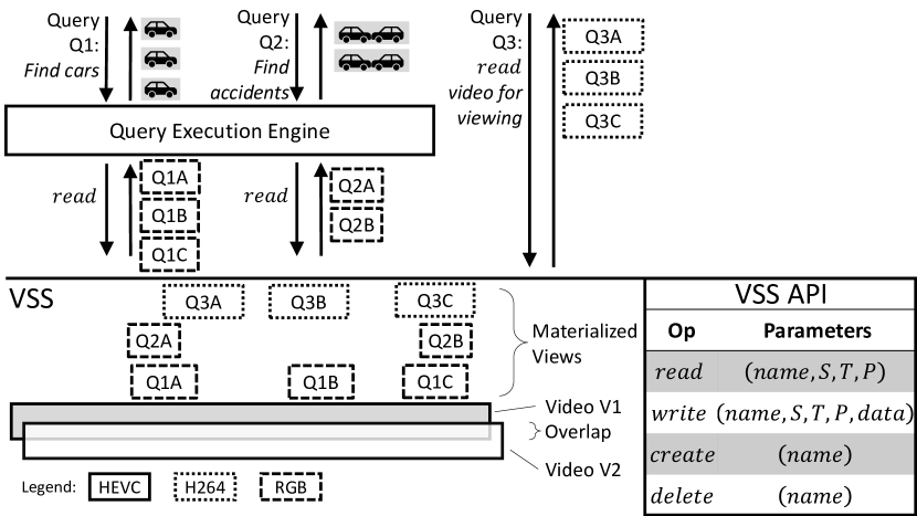
Figure 1. VSS overview & API. Reads and writes require specification of spatial ($S$; resolution, region of interest), temporal ($T$; start/end time, frame rate), and physical ($P$; frame layout, compression codec, quality) parameters.

The volume of video data captured and processed is rapidly increasing: YouTube receives more than 400 hours of uploaded video per minute (Wojcicki, 2018), and more than six million closed-circuit television cameras populate the United Kingdom, collectively amassing an estimated 7.5 petabytes of video per day (Cloudview, 2018). More than 200K body-worn cameras are in service (Hyland, 2018), collectively generating almost a terabyte of video per day (Yates, 2018).

To support this video data deluge, many systems and applications have emerged to ingest, transform, and reason about such data (Lu et al., 2016; Haynes et al., 2018; Jiang et al., 2018; Poms et al., 2018; Kang et al., 2019; Hsieh et al., 2018; Kang et al., 2017; Zhang et al., 2017). Critically, however, most of these systems lack efficient storage managers. They focus on query execution for a video that is already decoded and loaded in memory (Kang et al., 2017; Kang et al., 2019; Hsieh et al., 2018) or treat video compression as a black box (Lu et al., 2016; Jiang et al., 2018; Zhang et al., 2017) (cf. (Haynes et al., 2018; Poms et al., 2018)). In practice, of course, videos are stored on disk, and the cost of reading and decompressing is high relative to subsequent processing (Haynes et al., 2018; Daum et al., 2020), e.g., constituting more than 50% of total runtime (Kang et al., 2020). The result is a performance plateau limited by Amdahl’s law, where an emphasis on post-decompression performance might yield impressive results in isolation, but ignores the diminishing returns when performance is evaluated end-to-end.

In this paper, we develop VSS, a video storage system designed to serve as storage manager beneath a video data management system or video processing application (collectively VDBMSs). Analogous to a storage and buffer manager for relational data, VSS assumes responsibility for storing, retrieving, and caching video data. It frees higher-level components to focus on application logic, while VSS optimizes the low-level performance of video data storage. As we will show, this decoupling dramatically speeds up video processing queries and decreases storage costs. VSS does this by addressing the following three challenges:

First, modern video applications commonly issue multiple queries over the same (potentially overlapping) video regions and build on each other in different ways (e.g., Figure 1). Queries can also vary video resolution and other characteristics (e.g., the SMOL system rescales video to various resolutions (Kang et al., 2020) and Chameleon dynamically adjusts input resolution (Jiang et al., 2018)). Such queries can be dramatically faster with an efficient storage manager that maintains and evolves a cache of video data, each differently compressed and encoded.

Second, if the same video is queried using multiple systems such as via a VDBMS optimized for simple select and aggregate queries (Kang et al., 2019) and a separate vision system optimized for reasoning about complex scenes (Tsai et al., 2019) (e.g., Figure 1), then the video file may be requested at different resolutions and frame rates and using different encodings. Having a single storage system that encapsulates all such details and provides a unified query interface makes it seamless to create—and optimize—such federated workflows. While some systems have attempted to mitigate this by making multiple representations available to developers (Veeraraghavan et al., 2010; Xu et al., 2019), they expensively do so for entire videos even if only small subsets (e.g., the few seconds before and after an accident) are needed in an alternate representation.

Third, many recent applications analyze large amounts of video data with overlapping fields of view and proximate locations. For example, traffic monitoring networks often have multiple cameras oriented toward the same intersection and autonomous driving and drone applications come with multiple overlapping sensors that capture nearby video. Reducing the redundancies that occur among these sets of physically proximate or otherwise similar video streams is neglected in all modern VDBMSs. This is because of the substantial difficulties involved: systems (or users) need to consider the locations, orientations, and fields of view of each camera to identify redundant video regions; measure overlap, jitter, and temporally align each video; and ensure that deduplicated video data can be recovered with sufficient quality. Despite these challenges, and as we show herein, deduplicating overlapping video data streams offers opportunities to greatly reduce storage costs.

VSS addresses the above challenges. As a storage manager, it exposes a simple interface where VDBMSs read and write videos using VSS’s API (see Figure 1). Using this API, systems write video data in any format, encoding, and resolution—either compressed or uncompressed—and VSS manages the underlying compression, serialization, and physical layout on disk. When these systems subsequently read video—once again in any configuration and by optionally specifying regions of interest and other selection criteria—VSS automatically identifies and leverages the most efficient methods to retrieve and return the requested data.

VSS deploys the following optimizations and caching mechanisms to improve read and write performance. First, rather than storing video data on disk as opaque, monolithic files, VSS decomposes video into sequences of contiguous, independently-decodable sets of frames. In contrast with previous systems that treat video as static and immutable data, VSS applies transformations at the granularity of these sets of frames, freely transforming them as needed to satisfy a read operation. For example, if a query requests a video region compressed using a different codec, VSS might elect to cache the transcoded subregion and delete the original.

As VSS handles requests for video over time, it maintains a per-video on-disk collection of materialized views that is populated passively as a byproduct of read operations. When a VDBMS performs a subsequent read, VSS leverages a minimal-cost subset of these views to generate its answer. Because these materialized views can arbitrarily overlap and have complex interdependencies, finding the least-cost set of views is non-trivial. VSS uses a satisfiability modulo theories (SMT) solver to identify the best views to satisfy a request. VSS prunes stale views by selecting those least likely to be useful in answering subsequent queries. Among equivalently useful views, VSS optimizes for video quality and defragmentation.

Finally, VSS reduces the storage cost of redundant video data collected from physically proximate cameras. It does so by deploying a joint compression optimization that identifies overlapping regions of video and stores these regions only once. The key challenge lies in efficiently identifying potential candidates for joint compression in a large database of videos. Our approach identifies candidates efficiently without requiring any metadata specification. To identify video overlap, VSS incrementally fingerprints video fragments (i.e., it produces a feature vector that robustly characterizes video regions) and, using the resulting fingerprint index, searches for likely correspondences between pairs of videos. It finally performs a more thorough comparison between likely pairs.

In summary, we make the following contributions:

• We design a new storage manager for video data that leverages the fine-grained physical properties of videos to improve application performance (Section 2).

• We develop a novel technique to perform reads by selecting from potentially many materialized views to efficiently produce an output while maintaining the quality of the resulting video data (Section 3).

• We develop a method to optimize the storage required to persist videos that are highly overlapping or contain similar visual information, an indexing strategy to identify such regions (Section 5), and a protocol for caching multiple versions of the same video (Section 4).

We evaluate VSS against existing video storage techniques and show that it can reduce video read time by up to 54% and decrease storage requirements by up to 45% (Section 6).

2. VSS Overview

Consider an application that monitors an intersection for automobiles associated with missing children or adults with dementia. A typical implementation would first ingest video data from multiple locations around the intersection. It would then index regions of interest, typically by decompressing and converting the entire video to an alternate representation suitable for input to a machine learning model trained to detect automobiles. Many video query processing systems provide optimizations that accelerate this process (Kang et al., 2019; Lu et al., 2018; Xu et al., 2019). Subsequent operations, however, might execute more specific queries only on the regions that have automobiles. For example, if a red vehicle is missing, a user might issue a query to identify all red vehicles in the dataset. Afterward, a user might request and view all video sequences containing only the likely candidates. This might involve further converting relevant regions to a representation compatible with the viewer (e.g., at a resolution compatible with a mobile device or compressed using a supported codec). We show the performance of this application under VSS in Section 6.

While today’s video processing engines perform optimizations for operations over entire videos (e.g., the indexing phase described above), their storage layers provide little or no support for subsequent queries over the results (even dedicated systems such as quFiles (Veeraraghavan et al., 2010) or VStore (Xu et al., 2019) transcode entire videos, even when only a few frames are needed). Meanwhile, when the above application uses VSS to read a few seconds of low-resolution, uncompressed video data to find frames containing automobiles, it can delegate responsibility to VSS for efficiently producing the desired frames. This is true even if the video is streaming or has not fully been written to disk.

Critically, VSS automatically selects the most efficient way to generate the desired video data in the requested format and region of interest (ROI) based on the original video and cached representations. Further, to support real-time streaming scenarios, writes to VSS are non-blocking and users may query prefixes of ingested video data without waiting on the entire video to be persisted.

Figure 1 summarizes the set of VSS-supported operations. These operations are over logical videos, which VSS executes to produce or store fine-grained physical video data. Each operation involves a point- or range-based scan or insertion over a single logical video source. VSS allows constraints on combinations of temporal ($T$), spatial ($S$), and physical ($P$) parameters. Temporal parameters include start and end time interval ($[s,e]$) and frame rate ($f$); spatial parameters include resolution ($r_{x}\times r_{y}$) and region of interest ($[x_{0}..x_{1}]$ and $[y_{0}..y_{1}]$); and physical parameters $P$ include physical frame layout ($l$; e.g., yuv420, yuv422), compression method ($c$; e.g., hevc), and quality (to be discussed in Section 3.2).

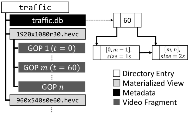
Figure 2. An example VSS physical organization that contains one logical video and two underlying physical videos. For physical video 1920x1080r30.hevc, the first $m$ GOPs are each one second in length, while the remaining $n-m$ are two seconds. These durations are recorded in the associated index.

Internally, VSS arranges each written physical video as a sequence of entities called groups of pictures (GOPs). Each GOP is composed of a contiguous sequence of frames in the same format and resolution. A GOP may include the full frame extent or be cropped to some ROI and may contain raw pixel data or be compressed. Compressed GOPs, however, are constrained such that they are independently decodable and take no data dependencies on other GOPs.

Though a GOP may contain an unbounded number of frames, video compression codecs typically fix their size to a small, constant number of frames (30–300) and VSS accepts as-is ingested compressed GOP sizes (which are typically less than 512kB). For uncompressed GOPs, our prototype implementation automatically partitions video data into blocks of size $\leq 25$MB (the size of one rgb 4K frame), or a single frame for resolutions that exceed this threshold.

Figure 2 illustrates the internal physical state of VSS. In this example, VSS contains a single logical video traffic with two physical representations (one hevc at $1920\times 1080$ resolution and 30 frames per second, and a 60-second variant at $960\times 540$ resolution). VSS has stored the GOPs associated with each representation as a series of separate files (e.g., traffic/1920x1080r30.hevc/1). It has also constructed a non-clustered temporal index that maps time to the file containing associated visual information. This level of detail is invisible to applications, which access VSS only through the operations summarized in Figure 1.

3. Data Retrieval from VSS

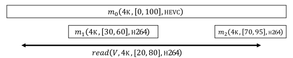
(a) Read operation on three materialized physical videos

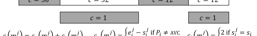
(b) Physical video fragments with simplified cost formulae

Figure 3. Figure 3(a) shows the query $read(V,4{\textsc{k}},$ $[20,80],\textsc{h264})$, where VSS has materialized $m_{0}$, $m_{1}$, and $m_{2}$. Figure 3(b) shows weighted fragments and costs. The lowest-cost result is shaded.

As mentioned, VSS internally represents a logical video as a collection of materialized physical videos. When executing a read, VSS produces the result using one or more of these views.

Consider a simplified version of the application described in Section 2, where a single camera has captured 100 minutes of 4K resolution, hevc-encoded video, and written it to VSS using the name $V$. The application first reads the entire video and applies a computer vision algorithm that identifies two regions (at minutes 30–60 and 70–95) containing automobiles. The application then retrieves those fragments compressed using h264 to transmit to a device that only supports this format. As a result of these operations, VSS now contains the original video ($m_{0}$) and the cached versions of the two fragments ($m_{1},m_{2}$) as illustrated in Figure 3(a). The figure indicates the labels $\{m_{0},m_{1},m_{2}\}$ of the three videos, their spatial configuration (4k), start and end times (e.g., $[0,100]$ for $m_{0}$), and physical characteristics (hevc or h264).

Later, a first responder on the scene views a one-hour portion of the recorded video on her phone, which only has hardware support for h264 decompression. To deliver this video, the application executes $read(V,\textsc{4k},[20,80],\textsc{h264})$, which, as illustrated by the arrow in Figure 3(a), requests video $V$ at 4k between time $[20,80]$ compressed with h264.

VSS responds by first identifying subsets of the available physical videos that can be leveraged to produce the result. For example, VSS can simply transcode $m_{0}$ between times $[20,80]$. Alternatively, it can transcode $m_{0}$ between time $[20,30]$ and $[60,70]$, $m_{1}$ between $[30,60]$, and $m_{2}$ between $[70,80]$. The latter plan is the most efficient since $m_{1}$ and $m_{2}$ are already in the desired output format (h264), hence VSS need not incur high transcoding costs for these regions. Figure 3(b) shows the different selections that VSS might make to answer this read. Each physical video fragment $\{f_{1},..f_{6}\}$ in Figure 3(b) represents a different region that VSS might select. Note that VSS need not consider other subdivisions—for example by subdividing $f_{5}$ at $[30,40]$ and $[40,60]$—since $f_{5}$ being cheaper at $[30,40]$ implies that it is at $[40,60]$ too.

To model these transcoding costs, VSS employs a transcode cost model $c_{t}(f,P,S)$ that represents the cost of converting a physical video fragment $f$ into a target spatial and physical format $S$ and $P$. The selected fragments must be of sufficient quality, which we model using a quality model $u(f,f^{\prime})$ and reject fragments of insufficient quality. We introduce these models in the following two subsections.

3.1. Cost Model

We first discuss how VSS selects fragments for use in performing a read operation using its cost model. In general, given a $read$ operation and a set of physical videos, VSS must first select fragments that cover the desired spatial and temporal ranges. To ensure that a solution exists, VSS maintains a cover of the initially-written video $m_{0}$ consisting of physical video fragments with quality equal to the original video (i.e., $u(m_{0},f)\geq\tau$). Our prototype sets a threshold $\tau=40$dB, which is considered to be lossless. See Section 3.2 for details. VSS also returns an error for reads extending outside of the temporal interval of $m_{0}$.

Second, when the selected physical videos temporally overlap, VSS must resolve which physical video fragments to use in producing the answer in a way that minimizes the total conversion cost of the selected set of video fragments. This problem is similar to materialized view selection (Halevy, 2001). Fortunately, a VSS read is far simpler than a general database query, and in particular is constrained to a small number of parameters with point- or range-based predicates.

We motivate our solution by continuing our example from Figure 3(a). First, observe that the collective start and end points of the physical videos form a set of transition points where VSS can switch to an alternate physical video. In Figure 3(a), the transition times include those in the set $\{30,60,70\}$, and we illustrate them in Figure 3(b) by partitioning the set of cached materialized views at each transition point. VSS ignores fragments that are outside the read’s temporal range, since they do not provide information relevant to the read operation.

Between each consecutive pair of transition points, VSS must choose exactly one physical video fragment. In Figure 3(b), we highlight one such set of choices that covers the read interval. Each choice of a fragment comes with a cost (e.g., $f_{1}$ has cost $32$), derived using a cost formula given by $c_{t}(f,P,S)=\alpha(f_{S},f_{P},S,P)\cdot|f|$. This cost is proportional to the total number of pixels $|f|$ in fragment $f$ scaled by $\alpha(S,P,S^{\prime},P^{\prime})$, which is the normalized cost of transcoding a single pixel from spatial and physical format $(S,P)$ into format $(S^{\prime},P^{\prime})$. For example, using fragment $m_{1}$ in Figure 3 requires transcoding from physical format $P=\textsc{hevc}$ to $P^{\prime}=\textsc{h264}$ with no change in spatiotemporal format (i.e., $S=S^{\prime}$).

During installation, VSS computes the domain of $\alpha$ by executing the vbench benchmark (Lottarini et al., 2018) on the installation hardware, which produces per-pixel transcode costs for a variety of resolutions and codecs. For resolutions not evaluated by vbench, VSS approximates $\alpha$ by piecewise linear interpolation of the benchmarked resolutions.

Figure 4. A simplified illustration based on Figure 3. VSS has decided to use $f_{1}$ and $f_{5}$ and is considering using $f_{3}$ starting at the red-highlighted frame. However, $f_{3}$ cannot be decoded without transitively decoding its dependencies shown by directed edges (labeled $\Delta$).

VSS must also consider the data dependencies between frames. Consider the illustration in Figure 4, which shows the frames within a physical video with their data dependencies indicated by directed edges. If VSS wishes to use a fragment at the frame highlighted in red, it must first decode all of the red frame’s dependent frames, denoted by the set $\Delta$ in Figure 4. This implies that the cost of transcoding a frame depends on where within the video it occurs, and whether its dependent frames are also transcoded.

To model this, we introduce a look-back cost $c_{l}(\Omega,f)$ that gives the cost of decoding the set of frames $\Delta$ on which fragment $f$ depends if they have not already been decoded, meaning that they are not in the set of previously selected frames $\Omega$. As illustrated in Figure 4, these dependencies come in two forms: independent frames $\mathrm{A}\subseteq\Delta$ (i.e., frames with out-degree zero in our graphical representation) which are larger in size but less expensive to decode, and the remaining dependent frames $\Delta-\mathrm{A}$ (those with outgoing edges) which are highly compressed but have more expensive decoding dependencies between frames. We approximate these per-frame costs using estimates from Costa et al. (Costa et al., 2018), which empirically concludes that dependent frames are approximately $45\%$ more expensive than their independent counterparts. We therefore fix $\eta=1.45$ and formalize look-back cost as $c_{l}(\Omega,f)=|\mathrm{A}-\Omega|+\eta\cdot|(\Delta-\mathrm{A})-\Omega|$.

To conclude our example, observe that our goal is to choose a set of physical video fragments that cover the queried spatiotemporal range, do not temporally overlap, and minimize the decode and look-back cost of selected fragments. In Figure 3(b), of all the possible paths, the one highlighted in gray minimizes this cost. These characteristics collectively meet the requirements identified at the beginning of this section.

Generating a minimum-cost solution using this formulation requires jointly optimizing both look-back cost $c_{l}$ and transcode cost $c_{t}$, where each fragment choice affects the dependencies (and hence costs) of future choices. These dependencies make the problem not solvable in polynomial time, and VSS employs an SMT solver (de Moura and Bjørner, 2008) to generate an optimal solution. Our embedding constrains frames in overlapping fragments so that only one is chosen, selects combinations of regions of interest (ROI) that spatially combine to cover the queried ROI, and uses information about the locations of independent and dependent frames in each physical video to compute the cumulative decoding cost due to both transcode and look-back for any set of selected fragments. We compare this algorithm to a dependency-naïve greedy baseline in Section 6.1.

3.2. Quality Model

Besides efficiency, VSS must also ensure that the quality of a result has sufficient fidelity. For example, using a heavily downsampled (e.g., $32\times 32$ pixels) or compressed (e.g., at a 1Kbps bitrate) physical video to answer a read requesting 4k video is likely to be unsatisfactory. VSS tracks quality loss from both sources using a quality model $u(f_{0},f)$ that gives the expected quality loss of using a fragment $f$ in a read operation relative to using the originally-written video $f_{0}$. When considering using a fragment $f$ in a read, VSS will reject it if the expected quality loss is below a user-specified cutoff: $u(f_{0},f)<\epsilon$. The user optionally specifies this cutoff in the read’s physical parameters (see Figure 1); otherwise, a default threshold is used ($\epsilon=40$dB in our prototype).

The range of $u$ is a non-negative peak signal-to-noise ratio (PSNR), a common measure of quality variation based on mean-squared error (Horé and Ziou, 2010). Values ${\geq}40$dB are considered to be lossless qualities, and ${\geq}30$dB near-lossless. PSNR is itself defined in terms of the mean-squared error (MSE) of the $n$ pixels in frame $f_{i}$ relative to the corresponding pixels in reference frame $f_{0}$, normalized by the maximum possible pixel value $I$ (generally 255):

$$PSNR(f_{i},f_{0})=\frac{1}{n}\sum_{j=0}^{n}10\cdot\log_{10}\big{(}\frac{I^{2}}{MSE(f_{i}[j],f_{0}[j])}\big{)}$$

As described previously, error in a fragment accumulates through two mechanisms—resampling and compression—and VSS uses the sum of both sources when computing $u$. We next examine how VSS computes error from each source.

Resampling error. First, for downsampled error produced through a resolution or frame rate change applied to $f_{0}$, computing $MSE(f,f_{0})$ is straightforward. However, VSS may transitively apply these transformations to a sequence of fragments. For example, $f_{0}$ might be downsampled to create $f_{1}$, and $f_{1}$ later used to produce $f_{2}$. In this case, when computing $MSE(f_{0},f_{2})$, VSS no longer has access to the uncompressed representation of $f_{0}$. Rather than expensively re-decompressing $f_{0}$, VSS instead bounds $MSE(f_{0},f_{n})$ in terms of $MSE(f_{0},f_{1}),...,MSE(f_{n-1},f_{n})$, which are a single real-valued aggregates stored as metadata. This bound is derived as follows for fragments of resolution $m\times n$:

$${MSE}(f_{0},f_{2}) =\frac{1}{mn}\sum_{i=0}^{m-1}\sum_{j=0}^{n-1}(f_{0}^{ij}-f_{2}^{ij})^{2}$$

$$=\frac{1}{mn}\sum_{i=0}^{m-1}\sum_{j=0}^{n-1}\big{[}(f_{0}^{ij}-f_{2}^{ij})^{2}+2(f_{1}^{ij})^{2}-2(f_{1}^{ij})^{2}$$

$$\phantom{====}+2f_{1}^{ij}f_{2}^{ij}-2f_{1}^{ij}f_{2}^{ij}+2f_{0}^{ij}f_{1}^{ij}-2f_{0}^{ij}f_{1}^{ij}\big{]}$$

$$=\frac{1}{mn}\sum_{i=0}^{m-1}\sum_{j=0}^{n-1}\begin{multlined}\big{[}(f_{0}^{ij}-f_{1}^{ij})^{2}+(f_{1}^{ij}-f_{2}^{ij})^{2}\\ +2f_{1}^{ij}(f_{2}^{ij}-f_{1}^{ij})-2f_{0}^{ij}(f_{2}^{ij}-f_{1}^{ij})\big{]}\\ \vspace{-1em}\end{multlined}\big{[}(f_{0}^{ij}-f_{1}^{ij})^{2}+(f_{1}^{ij}-f_{2}^{ij})^{2}\\ +2f_{1}^{ij}(f_{2}^{ij}-f_{1}^{ij})-2f_{0}^{ij}(f_{2}^{ij}-f_{1}^{ij})\big{]}\\ \vspace{-1em}$$

$$=\begin{multlined}MSE(f_{0},f_{1})+MSE(f_{1},f_{2})\\ +\frac{2}{mn}\sum_{i=0}^{m-1}\sum_{j=0}^{n-1}\big{[}(f_{1}^{ij}-f_{0}^{ij})\cdot(f_{2}^{ij}-f_{1}^{ij})\big{]}\\ \vspace{-1em}\end{multlined}MSE(f_{0},f_{1})+MSE(f_{1},f_{2})\\ +\frac{2}{mn}\sum_{i=0}^{m-1}\sum_{j=0}^{n-1}\big{[}(f_{1}^{ij}-f_{0}^{ij})\cdot(f_{2}^{ij}-f_{1}^{ij})\big{]}\\ \vspace{-1em}$$

$$=\begin{multlined}MSE(f_{0},f_{1})+MSE(f_{1},f_{2})\\ +\frac{2}{mn}\bigg{[}\sum_{i=0}^{m-1}\sum_{j=0}^{n-1}(f_{1}^{ij}-f_{0}^{ij})\cdot(f_{2}^{ij}-f_{1}^{ij})\cdot I(\cdot>0)+\\ \sum_{i=0}^{m-1}\sum_{j=0}^{n-1}(f_{1}^{ij}-f_{0}^{ij})\cdot(f_{2}^{ij}-f_{1}^{ij})\cdot I(\cdot<0)\bigg{]}\\ \vspace{-1em}\end{multlined}MSE(f_{0},f_{1})+MSE(f_{1},f_{2})\\ +\frac{2}{mn}\bigg{[}\sum_{i=0}^{m-1}\sum_{j=0}^{n-1}(f_{1}^{ij}-f_{0}^{ij})\cdot(f_{2}^{ij}-f_{1}^{ij})\cdot I(\cdot>0)+\\ \sum_{i=0}^{m-1}\sum_{j=0}^{n-1}(f_{1}^{ij}-f_{0}^{ij})\cdot(f_{2}^{ij}-f_{1}^{ij})\cdot I(\cdot<0)\bigg{]}\\ \vspace{-1em}$$

$$\leq\begin{multlined}MSE(f_{0},f_{1})+MSE(f_{1},f_{2})\\ +\frac{2}{mn}\sum_{i=0}^{m-1}\sum_{j=0}^{n-1}(f_{1}^{ij}-f_{0}^{ij})\cdot(f_{2}^{ij}-f_{1}^{ij})\cdot I(\cdot>0)\\ \vspace{-1em}\end{multlined}MSE(f_{0},f_{1})+MSE(f_{1},f_{2})\\ +\frac{2}{mn}\sum_{i=0}^{m-1}\sum_{j=0}^{n-1}(f_{1}^{ij}-f_{0}^{ij})\cdot(f_{2}^{ij}-f_{1}^{ij})\cdot I(\cdot>0)\\ \vspace{-1em}$$

$$\leq\begin{multlined}MSE(f_{0},f_{1})+MSE(f_{1},f_{2})\\ +\frac{2}{mn}\sum_{i=0}^{m-1}\sum_{j=0}^{n-1}\bigg{[}\frac{(f_{1}^{ij}-f_{0}^{ij})+(f_{2}^{ij}-f_{1}^{ij})}{2}\bigg{]}^{2}\\ \vspace{-1em}\end{multlined}MSE(f_{0},f_{1})+MSE(f_{1},f_{2})\\ +\frac{2}{mn}\sum_{i=0}^{m-1}\sum_{j=0}^{n-1}\bigg{[}\frac{(f_{1}^{ij}-f_{0}^{ij})+(f_{2}^{ij}-f_{1}^{ij})}{2}\bigg{]}^{2}\\ \vspace{-1em}$$

$$=\begin{multlined}MSE(f_{0},f_{1})+MSE(f_{1},f_{2})\\ +\frac{1}{2mn}\bigg{[}\sum_{i=0}^{m-1}\sum_{j=0}^{n-1}(f_{2}^{ij}-f_{0}^{ij})^{2}\cdot I(\cdot>0)\bigg{]}\\ \vspace{-1em}\end{multlined}MSE(f_{0},f_{1})+MSE(f_{1},f_{2})\\ +\frac{1}{2mn}\bigg{[}\sum_{i=0}^{m-1}\sum_{j=0}^{n-1}(f_{2}^{ij}-f_{0}^{ij})^{2}\cdot I(\cdot>0)\bigg{]}\\ \vspace{-1em}$$

$$\leq\begin{multlined}MSE(f_{0},f_{1})+MSE(f_{1},f_{2})+\frac{1}{2}MSE(f_{0},f_{2})\\ \vspace{-1em}\end{multlined}MSE(f_{0},f_{1})+MSE(f_{1},f_{2})+\frac{1}{2}MSE(f_{0},f_{2})\\ \vspace{-1em}$$

$$=2(MSE(f_{0},f_{1})+MSE(f_{1},f_{2}))$$

Using the above formulation, VSS efficiently estimates MSE for two transformations without requiring that the first fragment be available. Extension to transitive sequences is straightforward.

Compression error. Unlike resampling error, tracking quality loss due to lossy compression error is challenging because it cannot be calculated without decompressing—an expensive operation—and comparing the recovered version to the original input. Instead, VSS estimates compression error in terms of mean bits per pixel per second (MBPP/S), which is a metric reported during (re)compression. VSS then estimates quality by mapping MBPP/S to the PSNR reported by the vbench benchmark (Lottarini et al., 2018), a benchmark for evaluating video transcode performance in the cloud. To improve on this estimate, VSS periodically samples regions of compressed video, computes exact PSNR, and updates its estimate.

4. Data Caching in VSS

We now describe how VSS decides which physical videos to maintain, and which to evict under low disk space conditions. This involves making two interrelated decisions:

• When executing a read, should VSS admit the result as a new physical video for use in answering future reads?

• When disk space grows scarce, which existing physical video(s) should VSS discard?

To aid both decisions, VSS maintains a video-specific storage budget that limits the total size of the physical videos associated with each logical video. The storage budget is set when a video is created in VSS (see Figure 1) and may be specified as a multiple of the size of the initially written physical video or a fixed ceiling in bytes. This value is initially set to an administrator-specified default ($10{\times}$ the size of the initially-written physical video in our prototype). As described below, VSS ensures a sufficiently-high quality version of the original video can always be reproduced. It does so by maintaining a cover of fragments with sufficiently high quality (PSNR $\geq 40$dB in our prototype, which is considered to be lossless) relative to the originally ingested video.

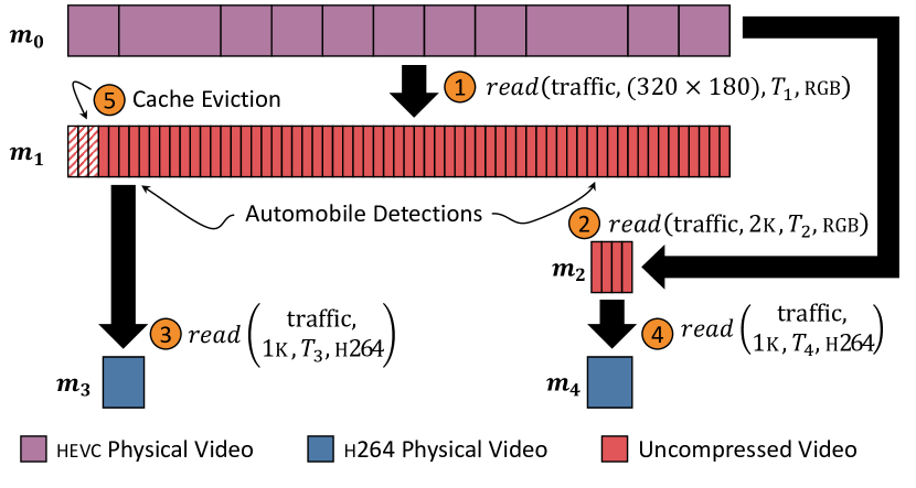
Figure 5. VSS caches read results and uses them to answer future queries. In an application reads traffic at $320{\times}180$ resolution for use in object detection, which VSS caches as $m_{1}$. In VSS caches $m_{2}$, a region with a dubious detection. In and VSS caches h264-encoded $m_{3}$ & $m_{4}$, where objects were detected. However, reading $m_{4}$ exceeds the storage budget and VSS evicts the striped region at .

As a running example, consider the sequence of reads illustrated in Figure 5, which mirrors the alert application described in Section 2. In this example, an application reads a low-resolution uncompressed video from VSS for use with an automobile detection algorithm. VSS caches the result as a sequence of three-frame GOPs (approximately 518kB per GOP). One detection was marginal, and so the application reads higher-quality 2K video to apply a more accurate detection model. VSS caches this result as a sequence of single-frame GOPs, since each 2K rgb frame is 6MB in size. Finally, the application extracts two h264-encoded regions for offline viewing. VSS caches $m_{3}$, but when executing the last read it determines that it has exceeded its storage budget and must now decide whether to cache $m_{4}$.

The key idea behind VSS’s cache is to logically break physical videos into “pages.” That is, rather than treating each physical video as a monolithic cache entry, VSS targets the individual GOPs within each physical video. Using GOPs as cache pages greatly homogenizes the sizes of the entries that VSS must consider. VSS’s ability to evict GOP pages within a physical video differs from other variable-sized caching efforts such as those used by content delivery networks (CDNs), which make decisions on large, indivisible, and opaque entries (a far more challenging problem space with limited solutions (Berger et al., 2018)).

However, there are several key differences between GOPs and pages. In particular, GOPs are related to each other; i.e., (i) one GOP might be a higher-quality version of another, and (ii) consecutive GOPs form a contiguous video fragment. These correlations make typical eviction policies like least-recently used (LRU) inefficient. In particular, naïve LRU might evict every other GOP in a physical video, decomposing it into many small fragments and increasing the cost of reads (which have exponential complexity in the number of fragments).

Additionally, given multiple, redundant GOPs that are all variations of one another, ordinary LRU would treat eviction of a redundant GOP the same as any other GOP. However, our intuition is that it is desirable to treat redundant GOPs different than singleton GOPs without such redundancy.

Given this intuition, VSS employs a modified LRU policy ($LRU_{VSS}$) that associates each fragment with a nonnegative sequence number computed using ordinary LRU offset by:

• Position ($p$). To reduce fragmentation, VSS increases the sequence number of fragments near the middle of a physical video, relative to the beginning or end. For a video with $n$ fragments arranged in ascending temporal order, VSS increases the sequence number of fragment $f_{i}$ by $p(f_{i})=\min(i,n-i)$.

• Redundancy ($r$). VSS decreases the sequence number of fragments that have redundant or higher-quality variants. To do so, using the quality cost model $u$, VSS generates a $u$-ordering of each fragment $f_{i}$ and all other fragments that are a spatiotemporal cover of $f_{i}$. VSS decreases the sequence number of $f_{i}$ by its rank $r(f_{i})\colon\mathbb{Z}^{0+}$ in this order (i.e., $r(f_{i})=0$ for a fragment with no higher-quality alternatives, while $r(f_{i})=n$ for a fragment with $n$ higher-quality variants).

• Baseline quality ($b$). VSS never evicts a fragment if it is the only fragment with quality equal to the quality of the corresponding fragment $m_{0}$ in the originally-written physical video. To ensure this, given a set of fragments $F$ in a video, VSS increases the sequence number of each fragment by (our prototype sets $\tau=40$):

  $$b(f_{i})=\begin{cases*}+\infty&if $\nexists f_{j}\in F\setminus f_{i}\ldotp u(m_{0},f_{j})\geq\tau$\\ 0&otherwise\end{cases*}$$

Using the offsets described above, VSS computes the sequence number of each candidate fragment $f_{i}$ as ${LRU}_{\textsc{vss}}(f_{i})=LRU(f_{i})+\gamma\cdot p(f_{i})-\zeta\cdot r(f_{i})+b(f_{i})$. Here weights $\gamma$ and $\zeta$ balance between position and redundancy, and our prototype weights the former ($\gamma=2$) more heavily than the latter ($\zeta=1$). It would be a straightforward extension to expose these as parameters tunable for specific workloads.

In Figure 5, we show application of ${LRU}_{\textsc{vss}}$ where VSS choses to evict the three-frame GOP at the beginning of $m_{1}$ and to cache $m_{4}$. If our prototype had instead weighed $\zeta\gg\gamma$, VSS would elect to evict $m_{3}$ since it was not recently used and is the variant with lowest quality.

5. Data Compression in VSS

As described in Section 2, when an application writes data to VSS, VSS partitions the written video into blocks by GOP (for compressed video data) or contiguous frames (for uncompressed video data). VSS follows the same process when caching the result of a read operation for future use.

VSS employs two compression-oriented optimizations and one optimization that reduces the number of physical video fragments. Specifically, VSS (i) jointly compresses redundant data across multiple physical videos (Section 5.1); (ii) lazily compresses blocks of uncompressed, infrequently-accessed GOPs (Section 5.2); and (iii) improves the read performance by compacting temporally-adjacent video (Section 5.3).

5.1. Joint Physical Video Compression

Increasingly large amounts of video content is produced from cameras that are spatially proximate with similar orientations. For example, a bank of traffic cameras mounted on a pole will each capture video of the same intersection from similar angles. Although the amount of “overlapping video” being produced is difficult to quantify, it broadly includes traffic cameras (7.5PB per day in the United Kingdom (Cloudview, 2018)), body-worn cameras (¿1TB per day (Yates, 2018)), autonomous vehicles (¿15TB per vehicle per hour (Heinrich and Motors, 2017)), along with videos of tourist locations, concerts, and political events. Despite the redundant information that mutually exists in these video streams, most applications treat these video streams as distinct and persist them separately to disk.

VSS optimizes the storage of these videos by reducing the redundancy between pairs of highly-similar video streams. It applies this joint compression optimization to pairs of GOPs in different logical videos. VSS first finds candidate GOPs to jointly compress. Then, given a pair of overlapping GOP candidates, VSS recompresses them frame-by-frame (we describe this process in Section 5.1.1). For static cameras, once VSS compresses the first frame in a GOP, it can reuse the information it has computed to easily compress subsequent frames in the same GOP. We describe joint compression for dynamic cameras in Section 5.1.2. We finally describe the search process for overlapping GOPs in Section 5.1.3.

(a) Frame from left video         

(b) Frame from right video   

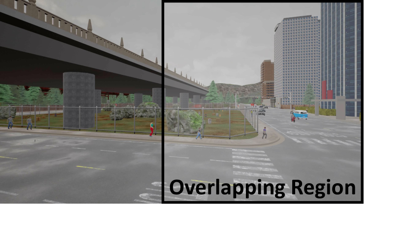
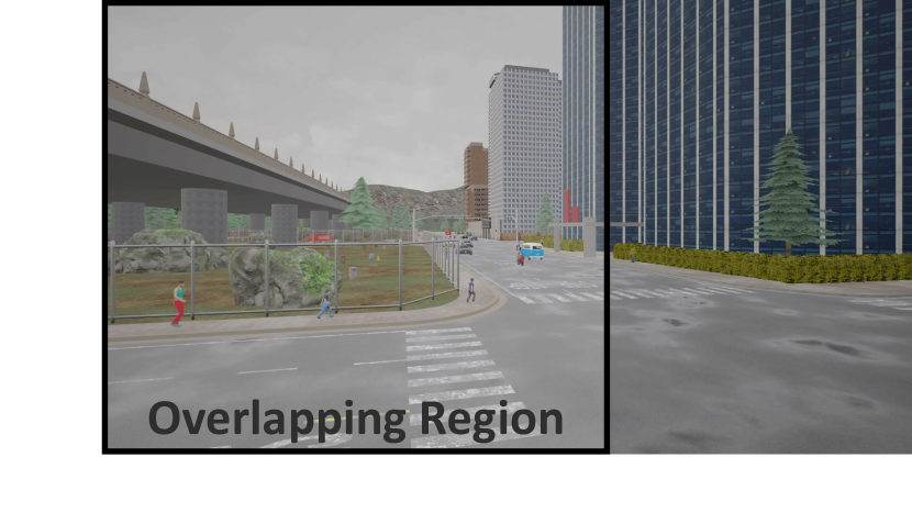
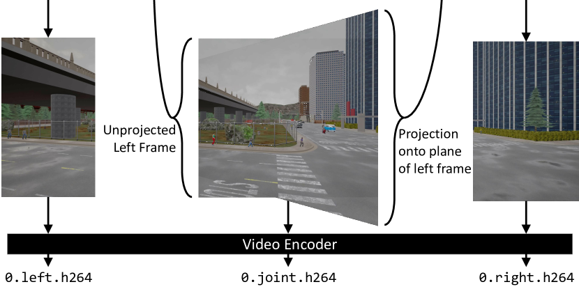
(c) Left, overlapped, and right regions are separately encoded.

Figure 6. The joint compression process. VSS identifies overlap, combines it, and separately encodes the pieces.

(a) Recovered frame from left video

(b) Recovered frame from right video

Figure 7. Recovered frames from joint compression.

(a) Original frame

(b) Recovered frame

Figure 8. An example recovered frame with slightly incorrect homography. In this case VSS detects the error relative to the original frame and aborts joint compression.

5.1.1. Joint frame compression

Figure 6 illustrates the joint compression process for two frames taken from a synthetic dataset (Visual Road-1K-50%, described in Section 6). Figures 6(a) and 6(b) respectively show the two frames with the overlap highlighted. Figure 6(c) shows the combined regions.

Because these frames were captured at different orientations, combining them is non-trivial and requires more than an isomorphic translation or rotation (e.g., the angle of the horizontal sidewalk is not aligned). Instead, VSS estimates a homography between the two frames and a projection is used to transform between the two spaces. As shown in Figure 6(c), VSS transforms the right frame, causing its right side to bulge vertically. However, after it is overlaid onto the left frame, the two align near-perfectly.

Algorithm 1 Joint compression algorithm

let $\textsc{homography}(f,g)$ estimate the $3{\times}3$ homography matrix of $f$ and $g$

let $u,\tau,\epsilon$ respectively be the VSS quality model (Section 3.2), quality

              threshold (Section 3.1), and duplicate threshold (Section 5.1.1).

function joint-compress($F,G,m$)

    Input: Video frames $F=\{f_{1},...,f_{n}\}$

    Input: Video frames $G=\{g_{1},...,g_{n}\}$

    Input: Merge function $m$

    Output: Vector of compressed subframes

    $H,C,i,j\leftarrow\textsc{homography}(f_{1},g_{1}),\emptyset,0,0$

    if $H=\emptyset$ then return $\emptyset$ $\triangleright$ No homography found00

    else if $H_{1,2}<0$ then return $\textsc{joint-compress}(G,F)$ $\triangleright$ Reverse transform00     

    while $i\leq n$ do

       if $\left||H-\mathcal{I}|\right|_{2}\leq\epsilon$ then

          $S_{i},H\leftarrow(\emptyset,f_{1},\emptyset),\mathcal{I}$ $\triangleright$ Duplicate Frames00000ll

       else

          $S_{i}\leftarrow\textsc{partition}(f_{i},g_{i},H,m)$        

       if $S_{i}=\emptyset\lor u\Big{(}f_{i},\big{[}S_{i}^{\text{left}}~{}S_{i}^{\text{overlap}}\big{]}\Big{)}<\tau~{}\lor$ $\triangleright$ Verify quality000000000l

            $u\Big{(}g_{i},\big{[}\textsc{transform}(S_{i}^{\text{overlap}},H^{-1})~{}S_{i}^{\text{right}}\big{]}\Big{)}<\tau$ then

          if j = 0 then $\triangleright$ Recompute homography

             $H,j\leftarrow\textsc{homography}(f_{i},g_{i}),j+1$

          else

             return $\emptyset$ $\triangleright$ Abort joint compression           

       else

          $C\leftarrow C\oplus\textsc{compress}(S_{i})$

          $i,j\leftarrow i+1,0$            

    return $C$

function partition($f,g,H,m$)

    Input: Video frame $f$ with size $n,m$

    Input: Video frame $g$ with size $n,m$

    Output: Left, overlap, and right subframes

    $x_{f}\leftarrow{\big{[}H^{-1}\cdot\begin{bmatrix}0&0&1\end{bmatrix}^{\intercal}\big{]}}_{2}$

    $x_{g}\leftarrow n-{\big{[}H\cdot\begin{bmatrix}n&0&1\end{bmatrix}^{\intercal}\big{]}}_{2}$

    if $\neg(0<x_{f}\leq n)\lor\neg(0<x_{g}\leq n)$ then $\textbf{return}~{}\emptyset$    

    $l,r\leftarrow f[1,x_{f}],g[x_{g},n]$ $\triangleright$ Left and right subframes

    $o\leftarrow m(f[x_{f},n],\textsc{transform}(g[1,x_{g}],H))$ $\triangleright$ Overlap of $f$ and $g$00000

    return $(l,o,r)$

function transform($f,H$) $\triangleright$ Compute perspective transform of $f$

    return $\begin{bmatrix}f^{\prime}_{1,1}&\ldots\\ \vdots&\ddots\end{bmatrix}$, where $t_{i,j}=H\cdot\begin{bmatrix}i\\ j\\ 1\end{bmatrix},~{}f^{\prime}_{i,j}=f_{\frac{[t_{i,j}]_{1}}{[t_{i,j}]_{3}},\frac{[t_{i,j}]_{2}}{[t_{i,j}]_{3}}}$

As formalized in Algorithm 1, joint projection proceeds as follows. First, VSS estimates a homography between two frames in the GOPs being compressed. Next, it applies a feature detection algorithm (Lowe, 1999) that identifies features that co-occur in both frames. Using these features, it estimates the homography matrix used to transform between frame spaces.

With a homography estimated, VSS projects the right frame into the space of the left frame. This results in three distinct regions: (i) a non-overlapping “left” region of the left frame, (ii) an overlapping region, and (iii) a “right” region of the right frame that does not overlap with the left. VSS splits these into three distinct regions and uses an ordinary video codec to encode each region separately and write it to disk.

When constructing the overlapping region, VSS applies a merge function that transforms overlapping pixels from each overlapping region and outputs a merged, overlapping frame. An unprojected merge favors the unprojected frame (i.e., the left frame in Figure 6(c)), while a mean merge averages the pixels from both input frames. During reads, VSS reverses this process to produce the original frames. Figure 7 shows two such recovered frames produced using the frames shown in Figure 6.

Some frames stored in VSS may be exact duplicates, however, for which the projection process described above introduces unnecessary computational overhead. VSS detects this case by checking whether the homography matrix would make a near-identity transform (specifically by checking $\left||H-\mathcal{I}|\right|\leq\epsilon$, where $\epsilon=\frac{1}{10}$ in our prototype). When this condition is met, VSS instead replaces the redundant GOP with a pointer to its near-identical counterpart.

5.1.2. Dynamic & mixed resolution cameras

For stationary and static cameras, the originally-computed homography is sufficient to jointly compress all frames in a GOP. For dynamic cameras, however, the homography quickly becomes outdated and, in the worst case, the cameras may no longer overlap. To guard against this, for each jointly compressed frame, VSS inverts the projection process and recovers the original frame. It then compares the recovered variant against the original using its quality model (see Section 3.2). If quality is too low ($<$24dB in our prototype), VSS re-estimates the homography and reattempts joint compression, and aborts if the reattempt is also of low quality.

For both static and dynamic cameras, VSS may occasionally poorly estimate the homography between two otherwise-compatible frames. The recovery process described above also identifies these cases. When detected (and if re-estimation is unsuccessful), VSS aborts joint compression for that pair of GOPs. An example of two frames where VSS produced an incorrect homography is illustrated in Figure 8.

VSS may also identify joint compression candidates that are at dissimilar resolutions. To handle this case, VSS first upscales the lower resolution fragment to that of the higher. It then applies joint compression as usual.

Figure 9. Joint compression fragment selection process: (i) compute and cluster fragment histograms, (ii) for the smallest cluster, compute features and search for fragments with many similar features, and (iii) for each pair, compute homography and (iv) compress.

5.1.3. Selecting GOPs for joint compression

Thus far we have discussed how VSS applies joint compression to a pair of GOPs, but not how the pairs are selected. Since the brute force approach of evaluating all $O(n^{2})$ pairs is prohibitively expensive, VSS instead uses the multi-step process illustrated in Figure 9. First, to reduce the search space, VSS clusters all video fragments using their color histograms. Videos with highly distinct color histograms are unlikely to benefit from joint compression. The VSS prototype implementation uses the BIRCH clustering algorithm (Zhang et al., 1996), which is memory efficient, scales to many data points, and allows VSS to incrementally update its clusters as new GOPs arrive.

Once VSS has clustered the ingested GOPs, it selects the cluster with the smallest radius and considers its constituents for joint compression. To do so, VSS applies a modified form of the homography computation described above. It begins by applying the feature detection algorithm (Lowe, 1999) from Section 5.1.1. Each feature is a spatial histogram characterizing an “interesting region” in the frame (i.e., a keypoint). VSS next looks for other GOPs in the cluster that share a large number of interesting regions. Thus, for each GOP, VSS iteratively searches for similar features (i.e., within distance $d$) located in other GOPs within the cluster. A correspondence, however, may be ambiguous (e.g., if a feature in GOP 1 matches to multiple, nearby features in GOP 2). VSS rejects such matches.

When VSS finds $m$ or more nearby, unambiguous correspondences, it considers the pair of GOPs to be sufficiently related. It then applies joint compression to the GOP pair as described above. Note that the algorithm described in Section 5.1.1 will abort if joint compressing the GOPs does not produce a sufficiently high-quality result. Our prototype sets $m=20$, requires features to be within $d=400$ (using a Euclidean metric), and disambiguates using Lowe’s ratio (Lowe, 2004).

5.2. Deferred Compression

Most video-oriented applications operate over decoded video data (e.g., rgb) that is vastly larger than its compressed counterpart (e.g., the VisualRoad-4K-30% dataset we describe in Section 6 is 5.2TB uncompressed as 8-bit rgb). Caching this uncompressed video quickly exhausts the storage budget.

To mitigate this, VSS adopts the following approach. When a video’s cache size exceeds a threshold (25% in our prototype), VSS activates its deferred compression mode. Thereafter when an uncompressed read occurs, VSS orders the video’s uncompressed cache entries by eviction order. It then losslessly compresses the last entry (i.e., the one least likely to be evicted). It then executes the read as usual.

Our prototype uses Zstandard for lossless compression, which emphasizes speed over compression ratio (relative to more expensive codecs such as PNG or HEVC) (Facebook, [n. d.]).

VSS performs two additional optimizations. First, Zstandard comes with a “compression level” setting in the range $[1..19]$, with the lowest setting having the fastest speed but the lowest compression ratio (and vice versa). VSS linearly scales this compression level with the remaining storage budget, trading off decreased size for increased throughput. Second, VSS also compresses cache entries in a background thread when no other requests are being executed.

5.3. Physical Video Compaction

While caching, VSS persists pairs of cached videos with contiguous time and the same spatial and physical configurations. (e.g., entries at time $[0,90]$ and $[90,120]$). Deferred compression may also create contiguous entries.

To reduce the number of videos that need to be considered during a read, VSS periodically and non-quiescently compacts pairs of contiguous cached videos and substitutes a unified representation. It does so by periodically examining pairs of cached videos and, for each contiguous pair, creating hard links from the second into the first. It then removes the second copy.

6. Evaluation

We have implemented a prototype of VSS in Python and C++ using CUDA (NVIDIA Corporation, 2007), NVENCODE (nvenc, 2020), OpenCV (OpenCV, 2018), FFmpeg (Bellard, 2018), and SQLite (SQLite Consortium, 2020). Our prototype adopts a no-overwrite policy and disallows updates. We plan on supporting both features in the future. Finally, VSS does not guarantee writes are visible until the file being written is closed.

Baseline systems. We compare against VStore (Xu et al., 2019), a recent storage system for video workloads, and direct use of the local file system. We build VStore with GPU support. VStore intermittently failed when operating on ${>}2,000$ frames and so we limit all VStore experiments to this size.

Experimental configuration. We perform all experiments using a single-node system equipped with an Intel i7 processor, 32GB RAM, and a Nvidia P5000 GPU.

Table 1. Datasets used to evaluate VSS

Dataset	Resolution	# Frames	Compressed
			Size (MB)
Robotcar	$1280{\times}960$	7,494	120
Waymo	$1920{\times}1280$	398	7
VisualRoad 1K-30%	$960{\times}540$	108k	224
VisualRoad 1K-50%	$960{\times}540$	108k	232
VisualRoad 1K-75%	$960{\times}540$	108k	226
VisualRoad 2K-30%	$1920{\times}1080$	108k	818
VisualRoad 4K-30%	$3840{\times}2160$	108k	5,500

Datasets. We evaluate using both real and synthetic video datasets (see Table 1). We use the former to measure VSS performance under real-world inputs, and the latter to test on a variety of carefully-controlled configurations. The “Robotcar” dataset consists of two highly-overlapping videos from vehicle-mounted stereo cameras (Maddern et al., 2017). The dataset is provided as 7,494 PNG-compressed frames at 30 FPS (as is common for datasets that target machine learning). We cropped and transcoded these frames into a h264 video with one-second GOPs.

The “Waymo” dataset is an autonomous driving dataset (waymo, 2020). We selected one segment ($\sim$20s) captured using two vehicle-mounted cameras. Unlike the Robotcar dataset, we estimate that Waymo videos overlap by $\sim$15%.

Finally, the various “VisualRoad” datasets consist of synthetic video generated using a recent video analytics benchmark designed to evaluate the performance of video-oriented data management systems (Haynes et al., 2019). To generate each dataset, we execute a one-hour simulation and produce video data at 1K, 2K, and 4K resolutions. We modify the field of view of each panoramic camera in the simulation so that we could vary the horizontal overlap of the resulting videos. We repeat this process to produce five distinct datasets; for example, “VisualRoad-1K-75%” has two 1K videos with 75% horizontal overlap.

Because the size of the uncompressed 4K Visual Road dataset ($\sim 5$TB) exceeds our storage capacity, we do not show results that require fully persisting this dataset uncompressed on disk.

6.1. Data Retrieval Performance

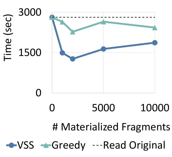
Figure 10. Time to select fragments and read video.

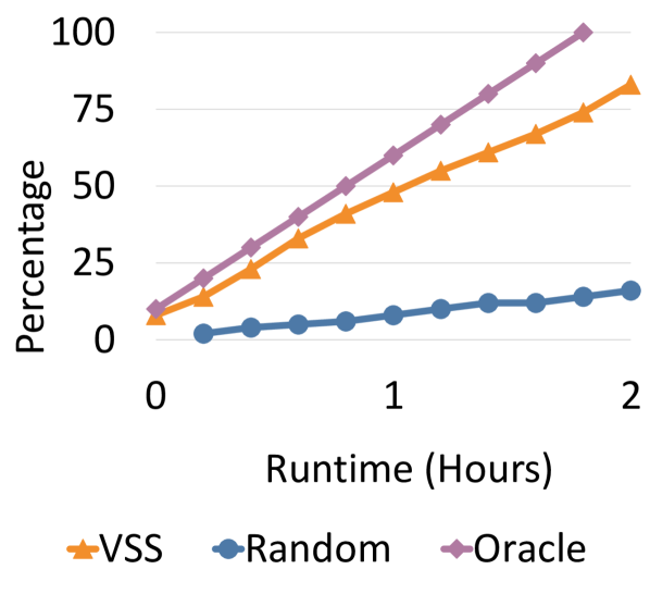
Figure 11. Joint compression pair selection.

Long Read Performance. We first explore VSS performance for large reads at various cache sizes. We repeatedly execute queries of the form $read(\text{VRoad-4K-30\%},4\textsc{k},[t_{1},t_{2}],P)$, with parameters drawn at random. We assume an infinite budget and iterate until VSS has cached a given number of videos.

We then execute a maximal hevc read ($t{=}[0\text{--}3600]$), which is different from the originally-written physical video (h264). This allows VSS to leverage its materialized fragments.

Figure 11 shows performance of this read. Since none of the other baseline systems support automatic conversion from h264 to hevc, we do not show their runtimes for this experiment.

As we see in Figure 11, even a small cache improves read performance substantially—28% at 100 entries and up to a maximum improvement of 54%. Further, because VSS decodes fewer dependent frames, VSS’s solver-based fragment selection algorithm outperforms both reading the original video and a naïve baseline that greedily selects fragments.

Short Read Performance. We next examine VSS performance when reading small, one-second regions of video (e.g., to apply license plate detection only to regions of video that contain automobiles). In this experiment, we begin with the VSS state generated by the previous experiment and execute many short reads of the form $read(\text{VisualRoad-4K-30\%},R,[t_{1},t_{2}],P)$, where $0\leq t_{1}<3600$ and $t_{2}=t_{1}+1$ (i.e., random 1 second sequences). $R$ and $P$ are as in the previous experiment.

Figure 13 shows the result for VSS (“VSS (All Optimizations)”) versus reading from the original video from the local file system (“Local FS”). For this experiment, VSS is able to offer improved performance due to its ability to serve from a cache of lower-cost fragments, rather than transcoding the source video. We discuss the other optimizations in this plot in Section 6.3.

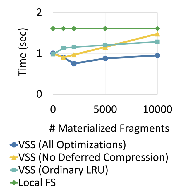
Figure 12. Selecting and reading short segments.

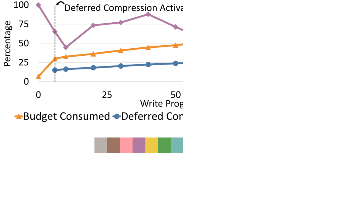
Figure 13. Writes with deferred compression.

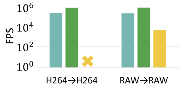
(a) Read in same format

(b) Read in different format

Figure 14. Read throughput. Each group $I{\rightarrow}O$ shows throughput reading in format $I$ and outputting in format $O$. An $\boldsymbol{\times}$ indicates lack of support for a read type.

Read Format Flexibility. Our next experiment evaluates VSS’s ability to read video data in a variety of formats. To evaluate, we write the VRoad-1K-30% dataset to each system in both compressed (224MB) and uncompressed form ($\sim$328GB). We then read video from each system in various formats and measure throughput. Figure 14 shows read results for the same (14(a)) and different (14(b)) formats. Because the local file system does not support automatic transcoding (e.g., h264 to rgb), we do not show results for these cases. Additionally, VStore does not support reading some formats; we we omit these cases.

We find that read performance without a format conversion from VSS is modestly slower than the local file system, due in part to the local file system being able to execute entirely without kernel transitions and VSS’s need to concatenate many individual GOPs. However, VSS can adapt to reads in any format, a benefit not available when using the local file system.

We also find that VSS outperforms VStore when reading uncompressed video and is similar when transcoding h264. Additionally, VSS offers flexible IO format options and does not require a workload to be specified in advance.

6.2. Data Persistence & Caching

(a) Uncompressed writes

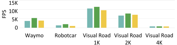
(b) Compressed writes (h264)

Figure 15. Throughput to write video.

Write Throughput. We next evaluate VSS write performance by writing each dataset to each system in both compressed and uncompressed form. For uncompressed writes, we measure throughput and show results in Figure 15(a).

For uncompressed datasets that fit on local storage, all systems perform similarly. On the other hand, no other systems have the capacity to store the larger uncompressed datasets (e.g., VisualRoad-4K-30% is $>$5TB uncompressed). However, VSS’s deferred compression allows it to store datasets no other system can handle (though with decreased throughput).

Figure 15(b) shows results for writing the compressed datasets to each store. Here all perform similarly; VSS and VStore exhibit minor overhead relative to the local file system.

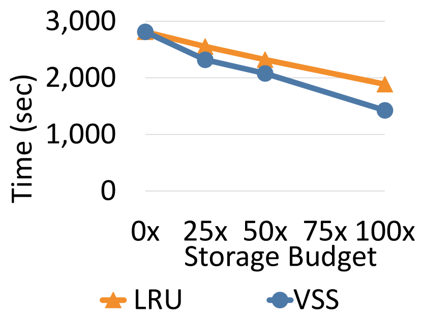
Figure 16. Read runtime by cache eviction policy.

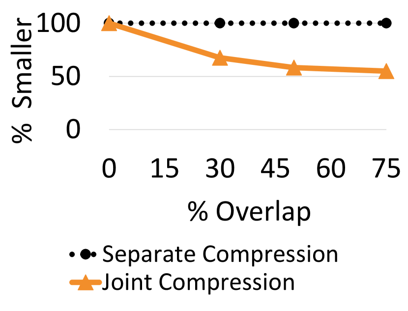
Figure 17. Joint compressed vs separate video.

Cache Performance. To evaluate the VSS cache eviction policy, we begin by executing 5,000 random reads to populate the cache, using the same parameters as in Section 6.1. In this experiment, instead of using an infinite storage budget, we limit it to multiples of the input size and apply either the least-recently used (LRU) or VSS eviction policy. This limits the number of physical videos available for reads. With the cache populated, we execute a final read for the entire video. Figure 17 plots runtimes for each policy and storage budget. This shows that VSS reduces read time relative to LRU.

6.3. Compression Performance

Table 2. Joint compression recovered quality

Dataset	Quality (PSNR)		Fragments
	Unprojected	Mean	Admitted (%)
	Left / Right	Left / Right	Unprojected / Mean
Robotcar	350 / 24	30 / 27	36 / 64
Waymo	352 / 29	32 / 30	39 / 68
VRoad-1K-30%	359 / 30	31 / 30	46 / 80
VRoad-1K-50%	358 / 28	29 / 29	41 / 72
VRoad-1K-75%	348 / 24	30 / 28	44 / 68
VRoad-2K-30%	352 / 30	30 / 30	52 / 82
VRoad-4K-30%	360 / 30	29 / 30	54 / 78

Joint Compression Quality. We first examine the recovered quality of jointly-compressed physical videos. For this experiment we write various overlapping Visual Road datasets to VSS. We then read each video back from VSS and compare its quality—using peak signal-to-noise ratio (PSNR)—against its originally-written counterpart.

Table 2 gives the PSNR for recovered data compared against the written videos. Recall that a PSNR of ${\geq}40$ is considered to be lossless, and ${\geq}30$ near-lossless (Horé and Ziou, 2010). When applying the unprojected merge function during joint compression, VSS achieves almost perfect recovery for the left input (with PSNR values exceeding 300dB) and near-lossless quality for the right input. Loss in fidelity occurs when inverting the merge, i.e., performing the inverse projection on the right frame using left-frame pixels decreases the quality of the recovered frame. This merge function also leads to VSS rejecting approximately half of the fragments due to their falling below the minimum quality threshold. We conclude this merge function is useful for reducing storage size in video data that must maintain at least one perspective in high fidelity.

On the other hand, VSS attains balanced, near-lossless quality for both the left and right frames when applying the mean merge function during joint compression. Additionally, the number of fragments admitted by the quality model is substantially higher under this merge function. Accordingly, the mean merge function is appropriate for scenarios where storage size is paramount and near-lossless degradation is acceptable.

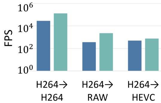
(a) Read throughput

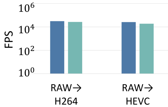
(b) Write throughput

Figure 18. Joint compression throughput.

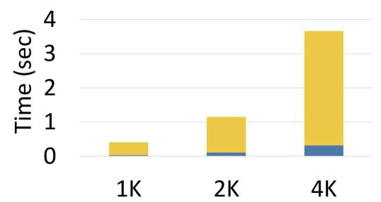
(a) By resolution

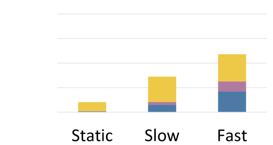
(b) By dynamicism

Figure 19. Joint compression overhead.

Joint Compression Throughput. We next examine read throughput with and without the joint compression optimization. First, we write the VisualRoad-1K-30% dataset to VSS, once with joint compression enabled and separately with it disabled. We then read in various physical configurations over the full duration. Figure 18(a) shows the throughput for reads using each configuration. Our results indicate that read overhead when using joint compression is modest but similar to reads that are not co-compressed.

Joint compression requires several nontrivial operations, and we next evaluate this overhead by writing 1k, 2k, and 4k video and measuring throughput. Figure 18(b) shows the results. Joint writes are similar to writing each video stream separately. This speedup is due to VSS’s encoding the lower-resolution streams in parallel. Additionally, the overhead in feature detection and generating the homography is low. Figure 19 decomposes joint compression overhead into these subcomponents. First, Figure 19(a) measures joint compression overhead by resolution, where compression costs dominate for all resolutions. Figure 19(b) further shows VSS performance under three additional scenarios: a static camera, a slowly rotating camera that requires homography reestimation every fifteen frames, and a rapidly rotating camera that requires reestimation every five frames. In these scenarios non-compression costs scale with the reestimation period, and compression performance is loosely correlated since a keyframe is needed after every homography change.

We next evaluate VSS’s joint compression selection algorithm. Using VisualRoad-1K-30%, we count joint compression candidates using (i) VSS’s algorithm, (ii) an oracle, and (iii) random selection. Figure 11 shows performance of each strategy. VSS identifies 80% of the applicable pairs in time similar to the oracle and outperforms random sampling.

Joint Compression Storage. To show the storage benefit of VSS’s joint compression optimization, we separately apply the optimization to each of the Visual Road videos. We then measure the final on-disk size of the videos against their separately-encoded variants. Figure 17 shows the result of this experiment. These results show joint compression substantially reduces the storage requirements of overlapping video.

Deferred Compression Performance. We next evaluate deferred compression for uncompressed writes by storing 3600 frames of the VisualRoad-1K-30% dataset in VSS, leaving budget and deferred compression at their defaults.

The results are listed in Figure 13. The figure shows storage used as a percentage of the budget, throughput relative to writing without deferred compression activated, and compression level. Storage used exceeds the deferred compression threshold early in the write, and a slope change shows that deferred compression is moderating write size. Compression level scales linearly with storage cost. Throughput drops substantially as compression is activated, recovers considerably, and then slowly degrades as the level is increased.

Similarly, Figure 21 shows throughput for reading fragments of raw video compressed at various levels. Though these reads have decreased performance and increased variance relative to uncompressed reads, at all levels ZStandard decompression remains much faster than using traditional video codecs.

Finally, Figure 13 explores the trade-offs between deferred compression performance and VSS’s cache eviction policy. In this experiment we variously disable deferred compression (“VSS (No Deferred Compression)”) and modify VSS to use ordinary LRU (“VSS (Ordinary LRU)”). The results show that VSS benefits from its eviction policy for small numbers of fragments (when deferred compression is off or at a low level) but offers increasingly large benefits as the cache grows. At large cache sizes as the storage budget is exhausted, deferred compression is increasingly important to mitigate eviction of fragments that are subsequently useful.

XXX XXX XXX XXX XXX XXX XXX

6.4. End-to-End Application Performance

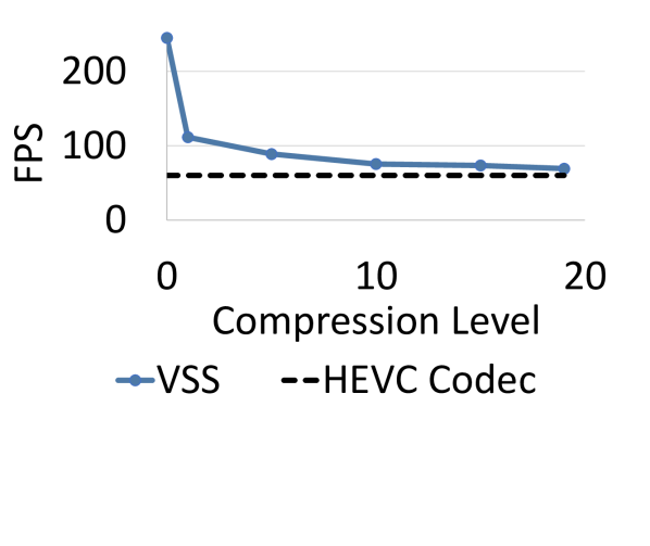
Figure 20. Throughput for reads over fragments with deferred compression.

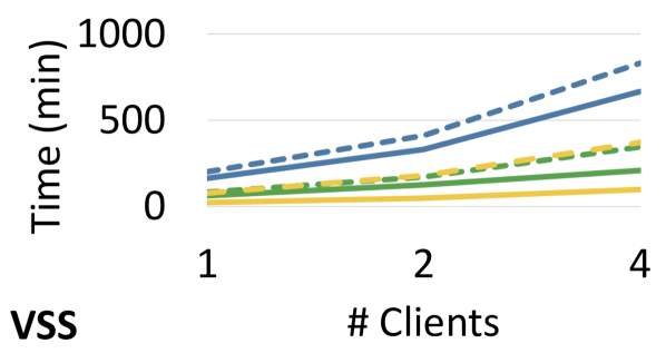
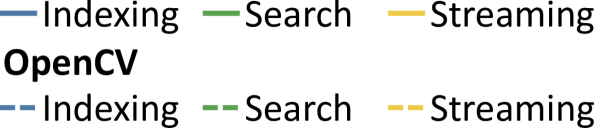
Figure 21. End-to-end application performance.

Our final experiment evaluates the performance of the end-to-end application described in Section 2. In this scenario, VSS serves as the storage manager for an application monitoring an intersection for automobiles. It involves three steps: (i) an indexing phase that identifies video frames containing automobiles using a machine learning algorithm, (ii) a search phase that, given an alert for a missing vehicle, uses the index built in the previous step to query video frames containing vehicles with matching colors, and (iii) a streaming content retrieval phase that uses the search phase results to retrieve video clips containing vehicles of a given color.

We implement this application using VSS and a variant that reads video data using OpenCV and the local file system. For indexing, the application identifies automobiles using YOLOv4 (Bochkovskiy et al., 2020) (both variants use OpenCV to perform inference using this model). For the search task, vehicle color is identified by computing a color histogram of the region inside the bounding box. We consider a successful detection to occur when the Euclidean distance between the largest bin and the search color is $\leq 50$. In the content retrieval phase, the application generates $n$ video clips by retrieving contiguous frames containing automobiles of the search color.

We use as input four extended two-hour variants of the Visual Road 2k dataset. To simulate execution by multiple clients, we launch a separate process for each client. Both variants index automobiles every ten frames (i.e., three times a second). All steps exhaust all CPU resources at $>4$ clients, and so we limit concurrent requests to this maximum.

Figure 21 shows the performance of each application step. The indexing step is a CPU-intensive operation that necessitates both video decoding and model inference, and because VSS introduces low overhead for reads, both variants perform similarly. Conversely, VSS excels at executing the search step, which requires retrieving raw, uncompressed frames that were cached during the indexing step. As such, it substantially outperforms the OpenCV variant. Finally, VSS’s ability to efficiently identify the lowest-cost transcode solution enables it to execute the streaming content retrieval step significantly faster than the OpenCV variant. We conclude that VSS’s performance greatly improves end-to-end application performance for queries that depend on cached video in multiple formats, and scales better with multiple clients.

7. Related Work

Increased interest in machine learning and computer vision has led to the development of a number of systems that target video analytics, including LightDB (Haynes et al., 2018), VisualWorldDB (Haynes et al., 2020), Optasia (Lu et al., 2016), Chameleon (Jiang et al., 2018), Panorama (Zhang and Kumar, 2019), Vaas (Bastani et al., 2020b), SurvQ (Stonebraker et al., 2020), and Scanner (Poms et al., 2018). These systems can be modified to leverage a storage manager like VSS. Video accelerators such as BlazeIt (Kang et al., 2019), VideoStorm (Zhang et al., 2017), Focus (Hsieh et al., 2018), NoScope (Kang et al., 2017), Odin (Suprem et al., 2020), SQV (Xarchakos and Koudas, 2019), MIRIS (Bastani et al., 2020a), Tahoma(Anderson et al., 2019), and Deluceva (Wang and Balazinska, 2020) can also benefit from VSS for training and inference.

Few recent storage systems target video analytics (although others have highlighted this need (Gupta-Cledat et al., 2017; Jiang et al., 2019)). VStore (Xu et al., 2019) targets machine learning workloads by staging video in pre-specified formats. However, VStore requires a priori knowledge of the workload and only makes preselected materializations available. By contrast, quFiles exploits data independence at the granularity of entire videos (Veeraraghavan et al., 2010). Others have explored on-disk layout of video for scalable streaming (Kang et al., 2009), and systems such as Haystack (Beaver et al., 2010), AWS Serverless Image Handler (Amazon, 2020), and VDMS (Remis et al., 2018) emphasize image and metadata operations.

Techniques similar to VSS’s joint compression optimization have been explored in the image and signal processing communities. For example, Melloni et al. develop a pipeline that identifies and aligns near-duplicate videos (Melloni et al., 2015), and Pinheiro et al. introduce a fingerprinting method to identify correlations among near-duplicate videos (Pinheiro et al., 2019). However, unlike VSS, these techniques assume that sets of near-duplicate videos are known a priori and they do not exploit redundancies to improve compression or read/write performance. Finally, the multiview extension to HEVC (MV-HEVC; similar extensions exist for other codecs) attempts to exploit spatial similarity in similar videos to improve compression performance (Hannuksela et al., 2015). These extensions are complementary to VSS, which could incorporate them as an additional compression codec for jointly-compressed video.

Finally, as in VSS, the database community has long exploited data independence to improve performance. Orthogonal optimizations could further improve VSS performance (e.g., perceptual compression (Mazumdar et al., 2019) or homomorphic operators (Haynes et al., 2018)).

8. Conclusion

We presented VSS, a video storage system that improves the performance of video-oriented applications. VSS decouples high-level operations (e.g., machine learning) from the low-level plumbing to read and write data in a suitable format. VSS automatically identifies the most efficient method to persist and retrieve video data. VSS reduces read time by up to 54%, and decreases the cost of persisting video by up to 45%.

As future work, we plan on extending VSS’s joint compression optimization to support more intelligent techniques for merging overlapping pixels. For example, VSS might intelligently detect occlusions and persist both pixels in these areas. This is important for cases where video must be maintained in its (near-)original form (e.g., for legal reasons).

Acknowledgments. This work is supported by the NSF through grants CCF-1703051, IIS-1546083, CCF-1518703, and CNS-1563788; DARPA award FA8750-16-2-0032 and RC Center grant GI18518; DOE award DE-SC0016260; a Google Faculty Research Award; an award from the University of Washington Reality Lab; a CoMotion Commercialization Fellows grant; gifts from the Intel Science and Technology Center for Big Data, Intel Corporation, Adobe, Amazon, Facebook, Huawei, and Google; and by CRISP, one of six centers in JUMP, a Semiconductor Research Corporation program sponsored by DARPA.

References

- (1)
- Amazon (2020) Amazon. 2020. Serverless Image Handler. https://aws.amazon.com/solutions/implementations/serverless-image-handler.
- Anderson et al. (2019) Michael R. Anderson, Michael J. Cafarella, German Ros, and Thomas F. Wenisch. 2019. Physical Representation-Based Predicate Optimization for a Visual Analytics Database. In ICDE. IEEE, 1466–1477.
- Bastani et al. (2020a) Favyen Bastani, Songtao He, Arjun Balasingam, Karthik Gopalakrishnan, Mohammad Alizadeh, Hari Balakrishnan, Michael J. Cafarella, Tim Kraska, and Sam Madden. 2020a. MIRIS: Fast Object Track Queries in Video. In SIGMOD. 1907–1921.
- Bastani et al. (2020b) Favyen Bastani, Oscar R. Moll, and Samuel Madden. 2020b. Vaas: Video Analytics at Scale. VLDB 13, 12 (2020), 2877–2880.
- Beaver et al. (2010) Doug Beaver, Sanjeev Kumar, Harry C. Li, Jason Sobel, and Peter Vajgel. 2010. Finding a Needle in Haystack: Facebook’s Photo Storage. In OSDI. 47–60.
- Bellard (2018) Fabrice Bellard. 2018. FFmpeg. https://ffmpeg.org.
- Berger et al. (2018) Daniel S. Berger, Nathan Beckmann, and Mor Harchol-Balter. 2018. Practical Bounds on Optimal Caching with Variable Object Sizes. POMACS 2, 2 (2018), 32:1–32:38.
- Bochkovskiy et al. (2020) Alexey Bochkovskiy, Chien-Yao Wang, and Hong-Yuan Mark Liao. 2020. YOLOv4: Optimal Speed and Accuracy of Object Detection. arXiv CoRR abs/2004.10934 (2020).
- Cloudview (2018) Cloudview. 2018. Visual IoT: Where the IoT Cloud and Big Data Come Together. http://www.cloudview.co/downloads/10. (2018).
- Costa et al. (2018) Victor H. Costa, Pedro A. Amado Assunção, and Paulo J. Cordeiro. 2018. A pixel-based complexity model to estimate energy consumption in video decoders. In ICCE. 1–5.
- Daum et al. (2020) Maureen Daum, Brandon Haynes, Dong He, Amrita Mazumdar, Magdalena Balazinska, and Alvin Cheung. 2020. TASM: A Tile-Based Storage Manager for Video Analytics. arXiv:2006.02958
- de Moura and Bjørner (2008) Leonardo Mendonça de Moura and Nikolaj Bjørner. 2008. Z3: An Efficient SMT Solver. In TACAS. 337–340.
- Facebook ([n. d.]) Facebook. [n. d.]. Zstandard real-time compression algorithm. https://facebook.github.io/zstd.
- Gupta-Cledat et al. (2017) Vishakha Gupta-Cledat, Luis Remis, and Christina R. Strong. 2017. Addressing the Dark Side of Vision Research: Storage. In HotStorage.
- Halevy (2001) Alon Y. Halevy. 2001. Answering queries using views: A survey. VLDB 10, 4 (2001), 270–294.
- Hannuksela et al. (2015) Miska M. Hannuksela, Ye Yan, Xuehui Huang, and Houqiang Li. 2015. Overview of the multiview high efficiency video coding (MV-HEVC) standard. In ICIP. 2154–2158.
- Haynes et al. (2020) Brandon Haynes, Maureen Daum, Amrita Mazumdar, Magdalena Balazinska, Alvin Cheung, and Luis Ceze. 2020. VisualWorldDB: A DBMS for the Visual World. In CIDR.
- Haynes et al. (2018) Brandon Haynes, Amrita Mazumdar, Armin Alaghi, Magdalena Balazinska, Luis Ceze, and Alvin Cheung. 2018. LightDB: A DBMS for Virtual Reality Video. PVLDB 11, 10 (2018), 1192–1205.
- Haynes et al. (2019) Brandon Haynes, Amrita Mazumdar, Magdalena Balazinska, Luis Ceze, and Alvin Cheung. 2019. Visual Road: A Video Data Management Benchmark. In SIGMOD. 972–987.
- Heinrich and Motors (2017) Stephan Heinrich and Lucid Motors. 2017. Flash memory in the emerging age of autonomy. Flash Memory Summit (2017).
- Horé and Ziou (2010) Alain Horé and Djemel Ziou. 2010. Image Quality Metrics: PSNR vs. SSIM. In ICPR. 2366–2369.
- Hsieh et al. (2018) Kevin Hsieh, Ganesh Ananthanarayanan, Peter Bodík, Shivaram Venkataraman, Paramvir Bahl, Matthai Philipose, Phillip B. Gibbons, and Onur Mutlu. 2018. Focus: Querying Large Video Datasets with Low Latency and Low Cost. In OSDI. 269–286.
- Hyland (2018) Shelley S Hyland. 2018. Body-worn cameras in law enforcement agencies, 2016. Bureau of Justice Statistics Publication No. NCJ251775 (2018).
- Jiang et al. (2018) Junchen Jiang, Ganesh Ananthanarayanan, Peter Bodík, Siddhartha Sen, and Ion Stoica. 2018. Chameleon: scalable adaptation of video analytics. In SIGCOMM. 253–266.
- Jiang et al. (2019) Junchen Jiang, Yuhao Zhou, Ganesh Ananthanarayanan, Yuanchao Shu, and Andrew A. Chien. 2019. Networked Cameras Are the New Big Data Clusters (HotEdgeVideo’19). 1–7.
- Kang et al. (2019) Daniel Kang, Peter Bailis, and Matei Zaharia. 2019. BlazeIt: Optimizing Declarative Aggregation and Limit Queries for Neural Network-Based Video Analytics. PVLDB 13, 4 (2019), 533–546.
- Kang et al. (2017) Daniel Kang, John Emmons, Firas Abuzaid, Peter Bailis, and Matei Zaharia. 2017. NoScope: Optimizing Deep CNN-Based Queries over Video Streams at Scale. PVLDB 10, 11 (2017), 1586–1597.
- Kang et al. (2020) Daniel Kang, Ankit Mathur, Teja Veeramacheneni, Peter Bailis, and Matei Zaharia. 2020. Jointly Optimizing Preprocessing and Inference for DNN-based Visual Analytics.
- Kang et al. (2009) Sooyong Kang, Sungwoo Hong, and Youjip Won. 2009. Storage technique for real-time streaming of layered video. MMSys 15, 2 (2009), 63–81.
- Lottarini et al. (2018) Andrea Lottarini, Alex Ramírez, Joel Coburn, Martha A. Kim, Parthasarathy Ranganathan, Daniel Stodolsky, and Mark Wachsler. 2018. vbench: Benchmarking Video Transcoding in the Cloud. In ASPLOS. 797–809.
- Lowe (1999) David G. Lowe. 1999. Object Recognition from Local Scale-Invariant Features. In ICCV. 1150–1157.
- Lowe (2004) David G. Lowe. 2004. Distinctive Image Features from Scale-Invariant Keypoints. IJCV 60, 2 (2004), 91–110.
- Lu et al. (2016) Yao Lu, Aakanksha Chowdhery, and Srikanth Kandula. 2016. Optasia: A Relational Platform for Efficient Large-Scale Video Analytics. In SoCC. 57–70.
- Lu et al. (2018) Yao Lu, Aakanksha Chowdhery, Srikanth Kandula, and Surajit Chaudhuri. 2018. Accelerating Machine Learning Inference with Probabilistic Predicates. In SIGMOD. 1493–1508.
- Maddern et al. (2017) Will Maddern, Geoff Pascoe, Chris Linegar, and Paul Newman. 2017. 1 Year, 1000km: The Oxford RobotCar Dataset. IJRR 36, 1 (2017), 3–15.
- Mazumdar et al. (2019) Amrita Mazumdar, Brandon Haynes, Magda Balazinska, Luis Ceze, Alvin Cheung, and Mark Oskin. 2019. Perceptual Compression for Video Storage and Processing Systems. In SoCC. 179–192.
- Melloni et al. (2015) Andrea Melloni, S. Lameri, Paolo Bestagini, Marco Tagliasacchi, and Stefano Tubaro. 2015. Near-duplicate detection and alignment for multi-view videos. In ICIP. 2444–2448.
- nvenc (2020) nvenc 2020. Nvidia Video codec. https://developer.nvidia.com/nvidia-video-codec-sdk.
- NVIDIA Corporation (2007) NVIDIA Corporation. 2007. NVIDIA CUDA Compute Unified Device Architecture Programming Guide. NVIDIA Corporation.
- OpenCV (2018) OpenCV. 2018. Open Source Computer Vision Library. https://opencv.org.
- Pinheiro et al. (2019) Giuliano Pinheiro, Marcos Cirne, Paolo Bestagini, Stefano Tubaro, and Anderson Rocha. 2019. Detection and Synchronization of Video Sequences for Event Reconstruction. In ICIP. 4060–4064.
- Poms et al. (2018) Alex Poms, Will Crichton, Pat Hanrahan, and Kayvon Fatahalian. 2018. Scanner: efficient video analysis at scale. TOG 37, 4 (2018), 138:1–138:13.
- Remis et al. (2018) Luis Remis, Vishakha Gupta-Cledat, Christina R. Strong, and Ragaad Altarawneh. 2018. VDMS: An Efficient Big-Visual-Data Access for Machine Learning Workloads. CoRR abs/1810.11832 (2018).
- SQLite Consortium (2020) SQLite Consortium. 2020. SQLite. https://www.sqlite.org.
- Stonebraker et al. (2020) Michael Stonebraker, Bharat Bhargava, Michael Cafarella, Zachary Collins, Jenna McClellan, Aaron Sipser, Tao Sun, Alina Nesen, KMA Solaiman, Ganapathy Mani, et al. 2020. Surveillance Video Querying with a Human-in-the-Loop. (2020).
- Suprem et al. (2020) Abhijit Suprem, Joy Arulraj, Calton Pu, and João Eduardo Ferreira. 2020. ODIN: Automated Drift Detection and Recovery in Video Analytics. VLDB 13, 11 (2020), 2453–2465.
- Tsai et al. (2019) Yao-Hung Hubert Tsai, Santosh Kumar Divvala, Louis-Philippe Morency, Ruslan Salakhutdinov, and Ali Farhadi. 2019. Video Relationship Reasoning Using Gated Spatio-Temporal Energy Graph. In CVPR. 10424–10433.
- Veeraraghavan et al. (2010) Kaushik Veeraraghavan, Jason Flinn, Edmund B. Nightingale, and Brian Noble. 2010. quFiles: The Right File at the Right Time. In FAST. 1–14.
- Wang and Balazinska (2020) Jingjing Wang and Magdalena Balazinska. 2020. Deluceva: Delta-Based Neural Network Inference for Fast Video Analytics. In SSDBM. 14:1–14:12.
- waymo (2020) waymo 2020. Waymo Open Dataset. https://waymo.com/open.
- Wojcicki (2018) Susan Wojcicki. 2018. The Potential Unintended Consequences of Article 13. https://youtube-creators.googleblog.com/2018/11/i-support-goals-of-article-13-i-also.html.
- Xarchakos and Koudas (2019) Ioannis Xarchakos and Nick Koudas. 2019. SVQ: Streaming Video Queries. In SIGMOD. 2013–2016.
- Xu et al. (2019) Tiantu Xu, Luis Materon Botelho, and Felix Xiaozhu Lin. 2019. VStore: A Data Store for Analytics on Large Videos. In EuroSys. 16:1–16:17.
- Yates (2018) Billy Yates. 2018. Body Worn Cameras: Making Them Mandatory. (2018).
- Zhang et al. (2017) Haoyu Zhang, Ganesh Ananthanarayanan, Peter Bodík, Matthai Philipose, Paramvir Bahl, and Michael J. Freedman. 2017. Live Video Analytics at Scale with Approximation and Delay-Tolerance. In NSDI. 377–392.
- Zhang et al. (1996) Tian Zhang, Raghu Ramakrishnan, and Miron Livny. 1996. BIRCH: An Efficient Data Clustering Method for Very Large Databases. In SIGMOD. 103–114.
- Zhang and Kumar (2019) Yuhao Zhang and Arun Kumar. 2019. Panorama: A Data System for Unbounded Vocabulary Querying over Video. VLDB 13, 4 (2019), 477–491.