A Sublattice Phase-Field Model for Direct CALPHAD Database Coupling

Abstract

The phase-field method has been established as a de facto standard for simulating the microstructural evolution of materials. In quantitative modeling the assessment and compilation of thermodynamic/kinetic data is largely dominated by the CALPHAD approach, which has produced a large set of experimentally and computationally generated Gibbs free energy and atomic mobility data in a standardized format: the thermodynamic database (TDB) file format. Harnessing this data for the purpose of phase-field modeling is an ongoing effort encompassing a wide variety of approaches. In this paper, we aim to directly link CALPHAD data to the phase-field method, without intermediate fitting or interpolation steps. We introduce a model based on the Kim-Kim-Suzuki (KKS) approach. This model includes sublattice site fractions and can directly utilize data from TDB files. Using this approach, we demonstrate the model on the U-Zr and Mo-Ni-Re systems.

1 Introduction

In the field of mesoscale materials modeling, the phase-field method has emerged as a well-established approach for simulating the coevolution of microstructure and properties [1, 2]. Describing the phase state and concentrations via field variables with finite-width smooth interfaces has proven an extremely flexible approach, resulting in a broad range of applications ranging from solidification [3, 4, 5] to phase transformation [6] to grain growth [7, 8].

Quantitative phase-field modeling of realistic material systems requires thermodynamic and kinetic input data in the form of Gibbs free energies and atomic mobilities. The assessment and compilation of such data through a combination of theoretical and experimental data are formalized by the CALPHAD approach [9]. In CALPHAD, Gibbs free energies are expressed as phenomenological function expansions combined with semi-empirical entropy models. As a standard machine-readable delivery format for these free energies, the thermodynamic database (TDB) ASCII-based file format was established. A large swath of open thermodynamic and kinetic data exists on the web and can be explored using search engines such as TDBDB [10].

Various indirect approaches exist to make this CALPHAD data available for phase-field modeling. Offline approaches utilize external thermodynamic software to precalculate the internal equilibration of site fractions. These precalculated free energies can be fitted to simple parabolas [11] or tabulated and interpolated over the entire state space. Tabulation can be performed on demand or on the fly to incrementally build the data, and tabulation approaches using polyadic tensor decomposition expansions [12] have been developed to address the explosion of the state space volume with increasing dimensionality. Zhang et al. [13] presented a direct coupling approach to multi-sublattice models, using an iterative two-step process to evolve phase-field variables and site fractions. A direct one-to-one relation between the variables in the CALPHAD database and those in the phase-field model is not established for models other than Type I $(A,B)_{k}(A)_{l}$.

The MOOSE framework [14, 15] contains functionality developed by the authors to extract the functional form of a free energy from TDB files. Direct usage of CALPHAD free energies in MOOSE-based phase-field simulations has so far been limited to models defined on a single sublattice (i.e., the substitutional solution model). The compound energy formalism [16, 17, 18] used in CALPHAD databases permits the description of phases with multiple sublattices, each with their own independent concentration degrees of freedom. Such a description is necessary to properly describe structurally complex intermetallic compounds such as the sigma phase in the Fe-Cr system [19]. Current phase-field models implemented in MOOSE, however, deal only in the overall composition of phases. The basic assumption for every material point is a local thermodynamic equilibrium.

Thermodynamic modeling software that uses multi-sublattice free energies must therefore perform a minimization of the internal degrees of freedom under the constraint of a given total overall concentration. The aim of this work is to derive a phase-field model that evolves the internal degrees of freedom in phases with multiple sublattices on-the-fly as part of a coupled partial differential equation system. As such, no preprocessing, tabulation, fitting, or approximation of the free energy density of the system must be performed. This method can therefore be used as a benchmark to quantify the errors inherent in preprocessing methods.

2 Sublattice KKS model

We recall that the original Kim-Kim-Suzuki (KKS) phase-field model [5] introduces the concept of phase concentrations $c_{ij}$ for every component $i$ and phase $j$ in the system. The phase concentrations are assumed to be in local thermodynamic equilibrium for each pair of phases $j$ and $j^{\prime}$:

$$\frac{\partial f_{j}}{\partial c_{ij}}=\frac{\partial f_{j^{\prime}}}{\partial c_{ij^{\prime}}}$$ (1)

where $f_{j}$ is a phase free energy density. The physical concentration $c_{i}$ for component $i$ is defined as:

$$c_{i}=\sum_{j}h_{j}c_{ij}$$ (2)

where $h_{j}$ represents switching functions that may depend on any combination of non-conserved order parameters $\eta_{j}$ and satisfies $\sum_{j}h_{j}=1$.

In a phase with multiple sublattices $k$, the phase concentrations $c_{ij}$ are split up into sublattice concentrations $c_{ijk}$, as per:

$$c_{ij}=\sum_{k}a_{jk}c_{ijk}$$ (3)

where $a_{jk}$ is a stoichiometric coefficient denoting the fraction of $k$ sublattice sites in phase $j$. The physical concentration for component $i$ is then written as:

$$c_{i}=\sum_{j}h_{j}\sum_{k}a_{jk}c_{ijk}$$ (4)

The sublattice concentrations enter the Allen-Cahn and Cahn-Hilliard equations only through their sum over all sublattcices in a given phase, the phase concentration. Thus the minimization of the total free energy requires each phase to have the minimum energy partitioning of the phase concentration onto its sublattices. That means the sublattice concentrations within a phase are given by a constrained minimization of the phase free energy density $f_{j}$. We use the Lagrange multiplier technique with the following constraint:

$$g_{ij}(\vec{c_{ij}})=\left[\sum_{k}a_{jk}c_{ijk}\right]-c_{ij}$$ (5)

where $\vec{c_{ij}}$ is the vector of $c_{ijk}$ for all $k$ and fixed $i$ and $j$. With the Lagrange multiplier $\lambda_{ij}$, we can write

$$\nabla_{\vec{c_{ij}}}f_{j}(\vec{c_{ij}})=\lambda_{ij}\nabla_{\vec{c_{ij}}}g_{ij}(\vec{c_{ij}})$$ (6)

where $\nabla_{\vec{c_{ij}}}$ is the differential operator of partial derivatives for the $\vec{c_{ij}}$ directions. Taking the component wise equality of the gradient vectors we obtain:

$$\frac{1}{a_{jk}}\frac{\partial f_{j}}{\partial c_{ijk}}=\lambda_{ij}\quad\forall k$$ (7)

Here, we pulled the stoichiometric coefficient $a_{jk}$ over to the left-hand side. This means that, for all sublattice pairs $k$ and $k^{\prime}$:

$$\frac{1}{a_{jk}}\frac{\partial f_{j}}{\partial c_{ijk}}=\frac{1}{a_{jk^{\prime}}}\frac{\partial f_{j}}{\partial c_{ijk^{\prime}}}$$ (8)

Taking the derivative of Eq. 3 with respect to the phase concentration $c_{ij}$ yields:

$$1=\sum_{k}a_{jk}\frac{\partial c_{ijk}}{\partial c_{ij}}$$ (9)

To obtain $\mu_{ij}$, the chemical potential of a constituent $i$ in phase $j$, we take the derivative of the phase free energy density $f_{j}$, with respect to the phase concentration $c_{ij}$:

$$\mu_{ij}=\frac{\partial f_{j}}{\partial c_{ij}}=\sum_{k}\frac{\partial f_{j}}{\partial c_{ijk}}\frac{\partial c_{ijk}}{\partial c_{ij}}$$ (10)

We can then substitute in eqs. 7 and 9 to obtain

$$\mu_{ij} =\sum_{k}\frac{1}{a_{jk}}\frac{\partial f_{j}}{\partial c_{ijk}}a_{jk}\frac{\partial c_{ijk}}{\partial c_{ij}}=\lambda_{ij}\sum_{k}a_{jk}\frac{\partial c_{ijk}}{\partial c_{ij}}$$ (11)

$$=\frac{1}{a_{jk}}\frac{\partial f_{j}}{\partial c_{ijk}}$$ (12)

where $k$ can be an arbitrary sublattice of phase $j$, as per Eq. 8. We note that, for phases containing only one sublattice, this model reduces to the original KKS model.

Note that at no point in the derivation do we require the stoichiometric coefficients $a_{jk}$ to sum up to one ($1=\sum_{k}a_{jk}$). This allows us to omit sublattices for constituents in certain phases if the constituent is not found in a given sublattice, as according to the CALPHAD model.

2.1 Evolution equations for an example three-phase system

To demonstrate the capability of the sublattice KKS phase-field model (SLKKS), we modified the three-phase KKS model originally described in [20] to include multiple sublattice concentrations. (However, it should be noted that the sublattice formulation is not restricted in any way to three-phase systems.) In this model, the three phases are represented by three order parameters ($\eta_{1}$, $\eta_{2}$, and $\eta_{3}$) constrained such that $\eta_{1}+\eta_{2}+\eta_{3}=1$. The total free energy density of the system $\mathcal{F}$ is given by:

$$\mathcal{F}=\int_{\Omega}\left[f_{\text{loc}}+f_{\text{gr}}\right]\text{d}V$$ (13)

where the local energy density $f_{\text{loc}}$ is given by:

$$f_{\text{loc}}=\sum_{j=1}^{3}h_{j}f_{j}+W\eta_{j}^{2}(1-\eta_{j})^{2}$$ (14)

and $W$ is the potential barrier height. The form of the switching function used for the three-phase system is described in Section 2.2. The gradient energy density $f_{\text{gr}}$ is given by:

$$f_{\text{gr}}=\sum_{j=1}^{3}\frac{\kappa}{2}\left|\nabla\eta_{j}\right|^{2}$$ (15)

To enforce the constraint $\eta_{1}+\eta_{2}+\eta_{3}=1$, a Lagrangian $\mathcal{F}_{L}$ is constructed based on Eq. 13:

$$\mathcal{F}_{L}=\int_{\Omega}\left[f_{\text{loc}}+f_{\text{gr}}+\lambda\left(1-\sum_{j=1}^{3}\eta_{i}\right)\right]\text{d}V$$ (16)

The Allen-Cahn equation for the evolution of each of the three phases is derived from the variational derivative of the Lagrangian:

$$\frac{\partial\eta_{i}}{\partial t}=-L\frac{\delta\mathcal{F}_{L}}{\delta\eta_{i}}$$ (17)

The full form of Eq. 17 is given in Ref. [21].

In [22], a further simplification of the Cahn-Hilliard equation in the KKS model is introduced, reducing the order of the partial differential equation to a modified diffusion problem. In MOOSE, this modification significantly improves the convergence of KKS multiphase simulations. The derivation by Kim et al. can be applied in straightforward fashion to the evolution equation, including the sublattice concentration, yielding:

$$\frac{\partial c_{i}}{\partial t}=\nabla\cdot D\sum_{j}h_{j}\sum_{k}a_{jk}\nabla c_{ijk}$$ (18)

We implemented Eqs. 3, 8, 17, and 18 in the C++Marmot [23] application, which is based on the MOOSE finite element framework [24].

2.2 Switching function

Crucial for the construction of a multiphase model is the choice of switching function $h_{j}$, which represents the physical phase fraction of a given phase $j$. A thermodynamically consistent switching function should not introduce artificial driving forces. In particular, the first derivative $\frac{\partial h_{j}}{\partial\eta_{j^{\prime}}}$ should be zero for any $j^{\prime}$ if $\eta_{j^{\prime}}=0$, with the second derivative being either positive or zero. This implies the absence of a driving force not strictly collinear with the edges of the Gibbs simplex defining the configurational phase space. Such a switching function prevents artificial formation of third phases along the interfaces of any two phases. We note that physically meaningful driving forces for the nucleation of new phases—resulting from the interplay of bulk free energy density and interfacial free energy—are unaffected by this choice.

A switching function that satisfies the aforementioned conditions for a three-phase system is the so-called “tilting function” defined by Folch and Plapp [25] as:

$$h^{\prime}_{j}(\eta_{j},\eta_{j^{\prime}},\eta_{j^{\prime\prime}})=\frac{\eta_{j}^{2}}{4}\left(15(1-\eta_{j})[1+\eta_{j}-(\eta_{j^{\prime\prime}}-\eta_{j^{\prime}})^{2}]\right.$$ (19)

$$\left.+\eta_{j}(9\eta_{j}^{2}-5)\right)$$

where $\eta_{j},\eta_{j^{\prime}},\eta_{j^{\prime\prime}}$ represents the cyclic rotations of the set of three order parameters associated with the three phases of the system.

We observe that numerical instability can arise from the formulation in 19, as $h^{\prime}_{j}$ can become either negative or larger than one for certain combinations of $\eta_{j},\eta_{j^{\prime}},\eta_{j^{\prime\prime}}$, resulting in unphysical phase fractions and divergent negative order parameters corresponding to phases with large free energies (such as line compound phases in composition space regions away from the compound stoichiometry). $h^{\prime}_{j}$ values outside of the interval $[0,1]$ require at least one order parameter to assume values outside the interval $[0,1]$. If an unconstrained partial differential equation (PDE) solver is used to evaluate the time evolution of the phase-field equations, the absence of physical barriers can lead the solve into these unphysical regions of the phase space.

To mitigate this problem, we propose a small modification of the tilting functions in order to effectively constrain the range of the function’s arguments by passing them through a soft Heaviside function $h^{\prime\prime}$ defined as:

$$h^{\prime\prime}(\eta)=\begin{cases}0,&\eta\leq 0\\ 3\eta^{2}-2\eta^{3},&0<\eta<1\\ 1,&1\leq\eta\end{cases}$$ (20)

Thus, we define $h_{j}=h^{\prime}_{j}\left(h^{\prime\prime}(\eta_{j}),h^{\prime\prime}(\eta_{j^{\prime}}),h^{\prime\prime}(\eta_{j^{\prime\prime}})\right)$, and, through application of the chain rule, it follows trivially that this formulation satisfies the condition of the absence of an artificial driving force.

3 Example applications

We use the Python package pycalphad [26] to read and parse TDB files. Pycalphad utilizes the SymPy [27] symbolic algebra Python package to construct abstract syntax trees (ASTs) of the free-energy expressions for each phase found in the TDB files. An AST is a tree data structure representing a mathematical expression, including all variables, operators, and functions used therein. We implemented a SymPy printer to output the free energy density expression AST in a text format compatible with the function expression parser [28] used in the MOOSE framework.

The resulting function expressions for the phase free energies as a function of their respective sublattice concentrations can be pasted directly into MOOSE input files. As laid out in [21], the expressions are then parsed at run time, and symbolic automatic differentiation is performed to obtain the expressions for the chemical potentials and derivatives needed to construct the Jacobian matrix of the problem. The free energy density expression and its derivatives are then transformed into executable machine code through just-in-time compilation for high-performance evaluation.

3.1 Uranium-zirconium

We demonstrate the sublattice KKS model on the binary uranium-zirconium system as assessed by Quaini et al. [29]. The TDB file for the system was obtained from the Thermodynamics of Advanced Fuel International Database [30].

At a temperature of 750 K, only the orthorhombic $\alpha$-uranium, hcp $\alpha$-zirconium, and $\delta$-UZr phases are stable. The former two phases are modeled using single sublattice models, while the $\delta$-UZr phase is described using the following sublattice model: $(U,Zr)_{k_{\delta,0}}(U,Zr)_{k_{\delta,1}}$ with $k_{\delta,0}=\frac{1}{3}$ and $k_{\delta,1}=\frac{2}{3}$.

When assembling the ideal mixing free energy density part of the AST, pycalphad inserts terms containing the product of site fraction $y_{i}$ and its logarithm as:

$$\begin{cases}y_{i}\log y_{i}&y_{i}>\epsilon_{y}\\ 0&y_{i}\leq\epsilon_{y}\end{cases}$$ (21)

where $\epsilon_{y}$ is a minimum site fraction constant defined as $10^{-16}$. While this procedure improves the numerical stability in pycalphad, it is detrimental in the finite-element-based implicit MOOSE solves. If during the solve, a site fraction value slips below $\epsilon_{y}$, the local chemical potential and its gradient switch to zero and do not contribute to a driving force that takes the site fraction back to physical values. This is illustrated in Fig. 1 (dashed curves), where a solve for the sublattice site fractions in the uranium-zirconium $\delta$-phase as a function of phase concentration results in unphysical sublattice populations with this definition of the ideal mixing free energy density. Instead, we replace the 21 terms with:

$$y_{i}\text{plog}(y_{i},\epsilon)$$ (22)

where plog is the natural logarithm for $y_{i}>\epsilon$ with $\epsilon>0$ and a Taylor expansion around $\epsilon$ for $y_{i}\leq\epsilon$, as defined in [21]. This substitution retains a strong driving force for unphysical site fractions and pushes the solve back into the physical regime while still avoiding the numerical issues associated with logarithms of negative numbers. The choice of $\epsilon$ is a trade-off in which a low $\epsilon$ increases the stiffness of the equation system but more faithfully retains the system’s thermodynamic properties. Fig. 1 (solid curves) shows the two sublattice concentrations for a successful constrained minimization of the $\delta$-UZr free energy density. To obtain this curve, we solve only Eqs. 3 and 8, and prescribe a linear concentration profile for the physical zirconium concentration $c_{Zr}$.

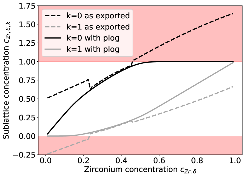
Figure 1: Sublattice concentrations in the uranium-zirconium $\delta$-phase as a function of phase concentration $c_{Zr,\delta}$. Shaded areas denote unphysical concentration regimes.

The resulting free energy density curve computed through the non-linear MOOSE solve is plotted in Fig. 2 (solid black line) on top of the pycalphad scatter plot that samples the entire sublattice concentration space. The MOOSE curve constitutes a lower bound (i.e., a constrained minimization of the the phase free energy density).

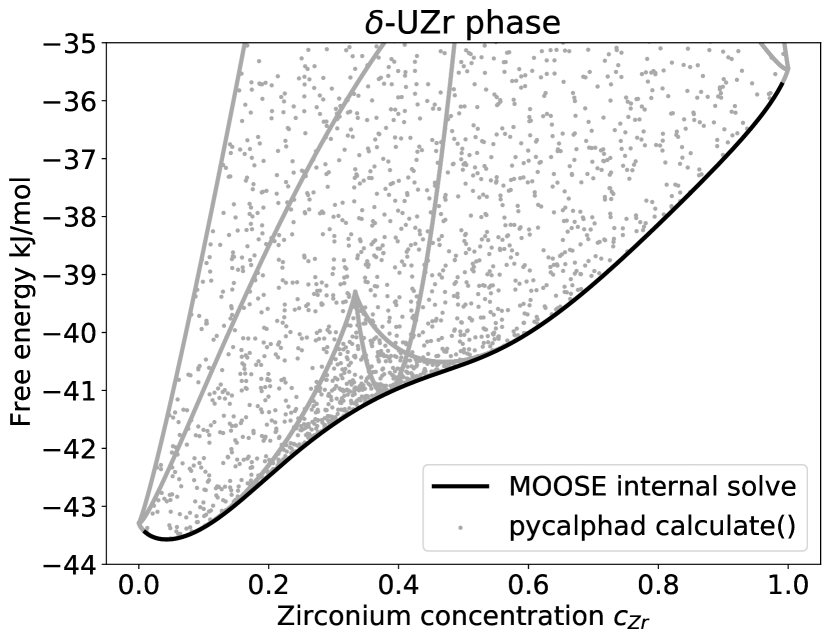
Figure 2: Free energy vs. $c_{Zr}$ for varying sublattice concentrations. The data points generated by pycalphad result from random sublattice concentration values that satisfy a particular value of $c_{Zr}$. The data generated by MOOSE result from the constrained minimization of the phase free energy density for each value of $c_{Zr}$. As is seen from the plot, the MOOSE constrained minimization accurately captures the lower bound of the pycalphad free-energy data.

To test the microstructural evolution of the UZr system within the SLKKS model, we set up a sharp uranium (left) / zirconium (right) interface. For all phases, we chose a gradient energy parameter $\kappa$ and barrier energy $W$ that resulted in an interfacial width of $\Omega_{U}^{\frac{1}{3}}$—where $\Omega_{U}$ is the atomic volume of a uranium atom in the $\alpha$-uranium phase—along with an interfacial free energy density of approximately 10 mJ/m². The selected interfacial free energy density was low enough to allow for spontaneous formation of the $\delta$-UZr phase. The atomic volumes of all three phases were set to $\Omega_{U}$. We note that atomic volume changes during phase transformations can be implemented through Eigenstrains, entailing a chemo-mechanical coupling. This will be the subject of future work and was left out in this study in order to focus on the chemical free-energy contribution enabled by the SLKKS model.

Figure 3 shows the evolution of the interfacial profile over time. The time units are arbitrary, and the diffusion coefficient $D$ was set to unity. The interface starts off sharp at $t_{0}$. The non-conserved order parameters are initialized with a sharp profile, as well. Within the first few time steps, the interface softens ($t_{1}$), and the interfacial profile determined by $\kappa$ and $W$ is established. At $t_{2}$, a nucleus of the $\delta$-UZr phase at a zirconium concentration of $\approx 0.65$ forms. We note that, at higher interfacial free energies, the nucleation of this phase is suppressed due to the energy barrier associated with the formation of an additional interface. At $t_{3}$, the $\delta$-UZr phase has further grown, consuming zirconium from the $\alpha$-zirconium phase on the right, which vanishes at $t_{4}$.

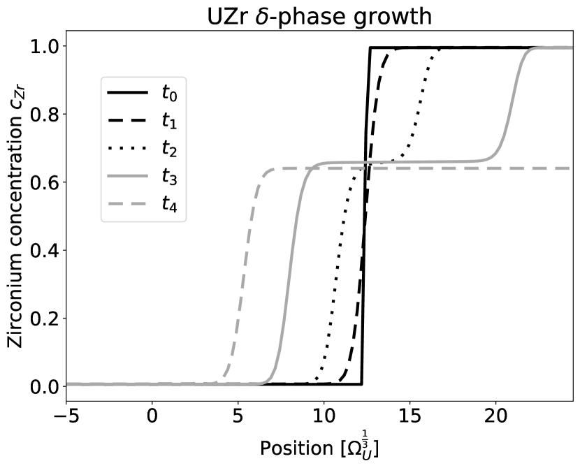
Figure 3: Evolution of the zirconium concentration at an initially ($t_{0}$) sharp uranium-zirconium interface. At time $t_{1}$, the interface profile evolves to the finite interface width of the phase-field model. At time $t_{2}$, a nucleus of the $\delta$-UZr phase at a zirconium concentration of $\approx 0.65$ forms. The $\delta$-UZr phase grows ($t_{3}$) and fully consumes the $\alpha$-Zr phase on the right as the simulation reaches equilibrium at $t_{4}$.

3.2 Molybdenum-nickel-rhenium

The Mo-Ni-Re system assessed by Yaqoob and Crivello et al. [31, 32] was chosen to demonstrate a ternary system with a particularly complex 5-sublattice model in the $\sigma$ phase with space group P42/mnm and a unit cell containing 30 atoms:

$$(Mo,Ni,Re)_{2}(Mo,Ni,Re)_{4}(Mo,Ni,Re)_{8}(Mo,Ni,Re)_{8}(Mo,Ni,Re)_{8}$$

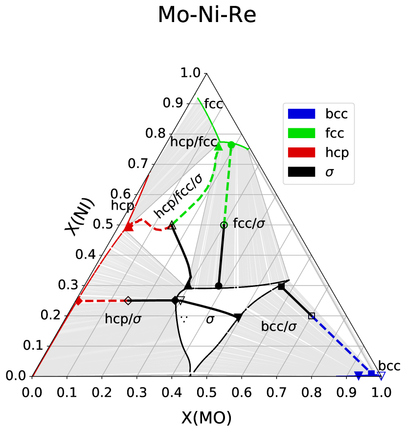
Figure 4: Phase diagram of the ternary Mo-Ni-Re system. Note the Ni-rich fcc phase, the Mo-poor hcp phase, and the Mo-rich bcc phase. Located near the center of the phase diagram is the sigma phase with its complex sublattice structure. The superimposed solid and dashed trajectories show the compositional evolution of phases tracked in multiple phase-field simulations. Empty symbols denote starting compositions, and filled symbols denote compositions evolved to equilibrium.

We selected the temperature to be 900 K, at which the hcp phase is only stable for molybdenum concentrations below about 3%. This permits us to construct (for demonstration purposes) two three-phase systems for which the thermodynamically consistent switching functions have already been derived: one system containing the fcc, bcc, and $\sigma$-phases, and one containing the fcc, hcp, and $\sigma$-phases. We again set the interface energy to 10 mJ/m², assigned the same mobility to all components, and set the same molar volume for each phase.

Figure 4 shows a phase diagram of the ternary Mo-Ni-Re system at 900 K and under ambient pressure, as plotted using pycalphad. On the phase diagram, we note the Ni-rich fcc phase, the Mo-poor hcp phase, and the Mo-rich bcc phase. Located near the center of the phase diagram is the $\sigma$-phase with its complex sublattice structure. Overlaid over the phase diagram are the compositional trajectories of five phase-field simulations.

The initial compositions for each run are denoted by the empty symbols. The filled symbols denote the final composition of each phase in the simulation. The phase concentration is determined by computing the weighted average value of each concentration variable, using the corresponding phase switching function value as the weight. A switching function is one, in the region the corresponding phase is active, and zero elsewhere. The interfacial regions can introduce a small error that becomes negligible for thin interfaces and a small interface-to-bulk ratio (i.e., a coarse microstructure). We note that, in this multiphase model, the non-conserved order parameters do not directly correspond to the phase fraction; instead, the above-mentioned switching functions—which are functions of all the non-conserved order parameters—represent the phase fractions.

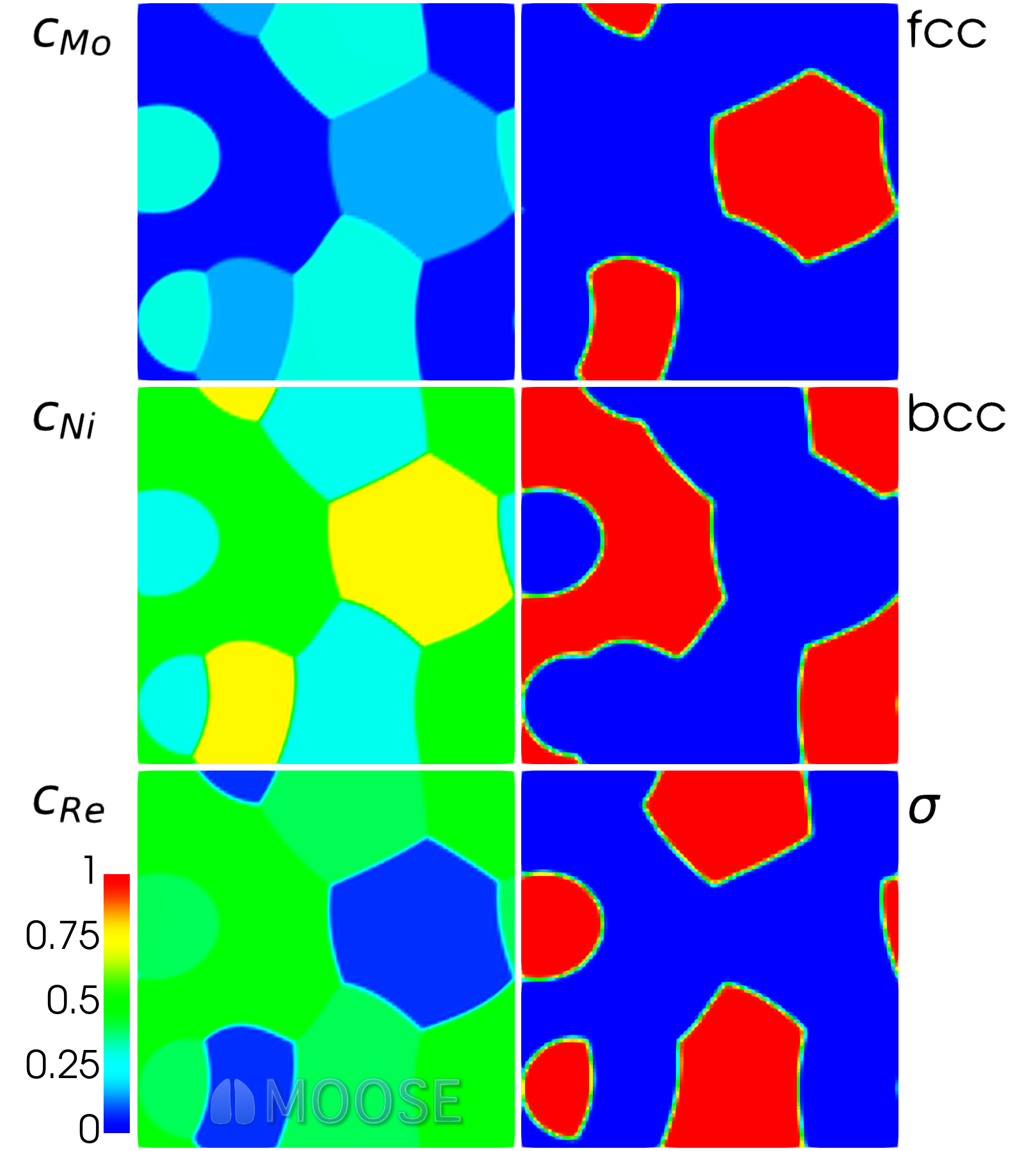
Figure 5: Phase separated microstructure evolved from a homogeneous initial composition of Mo₃Ni₁₀Re₇, which is located in the hcp, fcc, and $\sigma$-phase coexistence region.

All simulations were run with an interfacial free energy density of 10 mJ/m² and equal mobilities for all components, as this work deals with the free energy density of the bulk system. Interfacial effects and CALPHAD-informed mobilities will be the topic of future work.

A diffusion couple with a $\sigma$-phase and a bcc phase side (downward-pointing triangles) was set up with starting concentrations (open symbols) far inside the respective phase regions, with Mo₆Ni₅Re₉ in the $\sigma$-phase and pure molybdenum in the bcc phase. Through solute diffusion, the concentrations on both sides approach the respective phase boundaries in excellent agreement with the phase diagram. The underlying simulation was run in 1-D, thereby eliminating interface curvature effects.

Three two-phase decomposition simulations were run, with concentrations in the $\sigma$-fcc (circles), $\sigma$-bcc (squares), and $\sigma$-hcp (diamonds) coexistence regions, as denoted by the gray tie lines in the phase diagram. Each of the two-phase decomposition simulations was run in a finite-sized 2-D domain. The converged simulations show good agreement with the phase diagram boundaries. We note that the phase diagram does not take microstructural effects such as interfacial tensions into consideration; thus, perfect agreement is not expected.

A three-phase decomposition was run with a starting composition of Mo₃Ni₁₀Re₇, located in the hcp, fcc, and $\sigma$-phase coexistence region. An exemplary view of the ternary phase decomposition simulation microstructure is shown in Fig. 5, with the Mo, Ni, and Re (top to bottom) concentration order parameters on the left-hand side and the fcc, hcp, and $\sigma$-phase fraction on the right-hand side. In a finite-sized domain, a three-phase decomposition is not guaranteed to occur, as the energy penalty resulting from the formation of additional interfaces associated with a third phase can be prohibitively large.

4 Conclusions

As a natural extension of the KKS approach, we derived and demonstrated a phase-field model that tracks sublattice compositions and allows direct use of CALPHAD free energy models with multiple sublattices. The model, as presented, permits an arbitrary number of constituents and sublattices. The model is easily extendable to an arbitrary number of phases by utilizing the switching function proposed by Moelans et al. [33] or Pogorelov and Kundin et al. [34, 35], both of which suppress the formation of spurious phases at interfaces.

Data Availability

The thermodynamic data used in the example cases for this study are available online and can be accessed through TDBDB. The SLKKS model is implemented in the MOOSE[14] phase field module.

References

- [1] L.-Q. Chen, Phase-field models for microstructure evolution, Annual Review of Materials Research 32 (1) (2002) 113–140. doi:10.1146/annurev.matsci.32.112001.132041.
- [2] N. Moelans, B. Blanpain, P. Wollants, An introduction to phase-field modeling of microstructure evolution, CALPHAD 32 (2) (2008) 268–294. doi:10.1016/j.calphad.2007.11.003.
- [3] J. A. Warren, W. J. Boettinger, Prediction of dendritic growth and microsegregation patterns in a binary alloy using the phase-field method, Acta Metallurgica et Materialia 43 (2) (1995) 689–703. doi:10.1016/0956-7151(94)00285-P.
- [4] A. Karma, W.-J. Rappel, Phase-field method for computationally efficient modeling of solidification with arbitrary interface kinetics, Physical Review E 53 (4) (1996) R3017 (4 pages). doi:10.1103/PhysRevE.53.R3017.
-
[5]
S. G. Kim, W. T. Kim, T. Suzuki,
Phase-field model for
binary alloys, Physical Review E 60 (6) (1999) 7186–7197.
doi:10.1103/PhysRevE.60.7186.
URL http://link.aps.org/doi/10.1103/PhysRevE.60.7186 - [6] A. A. Wheeler, W. J. Boettinger, G. B. McFadden, Phase-field model for isothermal phase transitions in binary alloys, Physical Review A 45 (10) (1992) 7424–7439. doi:10.1103/PhysRevA.45.7424.
- [7] D. Fan, L.-Q. Chen, Diffusion-controlled grain growth in two-phase solids, Acta Materialia 45 (8) (1997) 3297–3310. doi:10.1016/S1359-6454(97)00022-0.
- [8] N. Moelans, B. Blanpain, P. Wollants, Quantitative analysis of grain boundary properties in a generalized phase field model for grain growth in anisotropic systems, Physical Review B 78 (2) (2008) 024113 (23 pages). doi:10.1103/PhysRevB.78.024113.
- [9] H. L. Lukas, S. G. Fries, B. Sundman, et al., Computational thermodynamics: the Calphad method, Vol. 131, Cambridge university press Cambridge, 2007.
-
[10]
A. van de Walle, C. Nataraj, Z.-K. Liu,
The
thermodynamic database database, Calphad 61 (2018) 173 – 178.
doi:https://doi.org/10.1016/j.calphad.2018.04.003.
URL http://www.sciencedirect.com/science/article/pii/S0364591618300099 -
[11]
A. Choudhury, M. Kellner, B. Nestler,
A
method for coupling the phase-field model based on a grand-potential
formalism to thermodynamic databases, Current Opinion in Solid State and
Materials Science 19 (5) (2015) 287 – 300.
doi:https://doi.org/10.1016/j.cossms.2015.03.003.
URL http://www.sciencedirect.com/science/article/pii/S135902861500025X -
[12]
Y. A. Coutinho, N. Vervliet, L. De Lathauwer, N. Moelans,
Combining thermodynamics
with tensor completion techniques to enable multicomponent microstructure
prediction, npj Computational Materials 6 (1) (2020) 2.
doi:10.1038/s41524-019-0268-y.
URL https://doi.org/10.1038/s41524-019-0268-y -
[13]
L. Zhang, M. Stratmann, Y. Du, B. Sundman, I. Steinbach,
Incorporating
the calphad sublattice approach of ordering into the phase-field model with
finite interface dissipation, Acta Materialia 88 (2015) 156 – 169.
doi:https://doi.org/10.1016/j.actamat.2014.11.037.
URL http://www.sciencedirect.com/science/article/pii/S1359645414008908 -
[14]
D. Gaston, C. Permann, D. Andrs, J. W. Peterson, A. Slaughter, J. Miller,
MOOSE Framework Web page (2015).
URL https://mooseframework.inl.gov - [15] C. J. Permann, D. R. Gaston, D. Andrs, R. W. Carlsen, F. Kong, A. D. Lindsay, J. M. Miller, J. W. Peterson, A. E. Slaughter, R. H. Stogner, R. C. Martineau, Moose: Enabling massively parallel multiphysics simulation (2019). arXiv:1911.04488.
- [16] M. Hillert, L.-I. Staffansson, The regular solution model for stoichiometric phases and ionic melts, Acta Chemica Scandinavica 24 (4) (1970) 3618–3626. doi:10.3891/acta.chem.scand.24-3618.
-
[17]
B. Sundman, J. Ågren,
A
regular solution model for phases with several components and sublattices,
suitable for computer applications, Journal of Physics and Chemistry of
Solids 42 (4) (1981) 297–301, cited By 761.
doi:10.1016/0022-3697(81)90144-X.
URL https://www.scopus.com/inward/record.uri?eid=2-s2.0-0019699113&doi=10.1016%2f0022-3697%2881%2990144-X&partnerID=40&md5=960218ec37af45447eecb912e7fa1c7e -
[18]
M. Hillert,
The
compound energy formalism, Journal of Alloys and Compounds 320 (2) (2001)
161 – 176, materials Constitution and Thermochemistry. Examples of Methods,
Measurements and Applications. In Memoriam Alan Prince.
doi:https://doi.org/10.1016/S0925-8388(00)01481-X.
URL http://www.sciencedirect.com/science/article/pii/S092583880001481X -
[19]
A. Jacob, E. Povoden-Karadeniz, E. Kozeschnik,
Revised
thermodynamic description of the fe-cr system based on an improved sublattice
model of the phase, Calphad 60 (2018) 16 – 28.
doi:https://doi.org/10.1016/j.calphad.2017.10.002.
URL http://www.sciencedirect.com/science/article/pii/S0364591617301116 - [20] M. Ohno, K. Matsuura, Quantitative phase-field modeling for two-phase solidification process involving diffusion in the solid, Acta Materialia 58 (17) (2010) 5749–5758. doi:10.1016/j.actamat.2010.06.050.
-
[21]
D. Schwen, L. Aagesen, J. Peterson, M. Tonks,
Rapid
multiphase-field model development using a modular free energy based approach
with automatic differentiation in MOOSE/MARMOT, Computational Materials
Science 132 (2017) 36–45.
doi:10.1016/J.COMMATSCI.2017.02.017.
URL https://www.sciencedirect.com/science/article/pii/S0927025617300885 -
[22]
S. Gyoon Kim, W. Tae Kim, T. Suzuki, M. Ode,
Phase-field
modeling of eutectic solidification, Journal of Crystal Growth 261 (1)
(2004) 135–158.
doi:10.1016/j.jcrysgro.2003.08.078.
URL https://linkinghub.elsevier.com/retrieve/pii/S0022024803017974 - [23] M. R. Tonks, D. Gaston, P. C. Millett, D. Andrs, P. Talbot, An object-oriented finite element framework for multiphysics phase field simulations, Computational Materials Science 51 (1) (2012) 20–29. doi:10.1016/j.commatsci.2011.07.028.
- [24] D. R. Gaston, C. J. Permann, J. W. Peterson, A. E. Slaughter, D. Andrš, Y. Wang, M. P. Short, D. M. Perez, M. R. Tonks, J. Ortensi, R. C. Martineau, Physics-based multiscale coupling for full core nuclear reactor simulation, Annals of Nuclear Energy, Special Issue on Multi-Physics Modelling of LWR Static and Transient Behaviour 84 (2015) 45–54. doi:10.1016/j.anucene.2014.09.060.
- [25] R. Folch, M. Plapp, Quantitative phase-field modeling of two-phase growth, Physical Review E 72 (1) (2005) 011602 (27 pages). doi:10.1103/PhysRevE.72.011602.
-
[26]
R. Otis, Z.-K. Liu,
pycalphad:
CALPHAD-based Computational Thermodynamics in Python, Journal of
Open Research Software 5 (Jan. 2017).
doi:10.5334/jors.140.
URL http://openresearchsoftware.metajnl.com/articles/10.5334/jors.140/ -
[27]
A. Meurer, C. P. Smith, M. Paprocki, O. Čertík, S. B. Kirpichev,
M. Rocklin, A. Kumar, S. Ivanov, J. K. Moore, S. Singh, T. Rathnayake,
S. Vig, B. E. Granger, R. P. Muller, F. Bonazzi, H. Gupta, S. Vats,
F. Johansson, F. Pedregosa, M. J. Curry, A. R. Terrel, v. Roučka,
A. Saboo, I. Fernando, S. Kulal, R. Cimrman, A. Scopatz,
SymPy: symbolic computing in
python, PeerJ Computer Science 3 (2017) e103.
doi:10.7717/peerj-cs.103.
URL https://doi.org/10.7717/peerj-cs.103 -
[28]
J. Nieminen, J. Yliluoma,
Function Parser Web
page (2011).
URL http://warp.povusers.org/FunctionParser -
[29]
A. Quaini, C. Guéneau, S. Gossé, N. Dupin, B. Sundman, E. Brackx,
R. Domenger, M. Kurata, F. Hodaj,
Contribution
to the thermodynamic description of the corium – the U-Zr-O system,
Journal of Nuclear Materials 501 (2018) 104 – 131.
doi:https://doi.org/10.1016/j.jnucmat.2018.01.023.
URL http://www.sciencedirect.com/science/article/pii/S0022311517313314 -
[30]
N. N. S. Committee,
Thermodynamics of
Advanced Fuels – International Database (TAF-ID) (2019).
URL https://www.oecd-nea.org/science/taf-id/ -
[31]
K. Yaqoob, J.-C. Crivello, J.-M. Joubert,
Comparison of the site occupancies
determined by combined rietveld refinement and density functional theory
calculations: Example of the ternary mo-ni-re phase, Inorganic Chemistry
51 (5) (2012) 3071–3078, pMID: 22356428.
arXiv:https://doi.org/10.1021/ic202479y, doi:10.1021/ic202479y.
URL https://doi.org/10.1021/ic202479y -
[32]
J.-C. Crivello, R. Souques, A. Breidi, N. Bourgeois, J.-M. Joubert,
ZenGen,
a tool to generate ordered configurations for systematic first-principles
calculations: The cr–mo–ni–re system as a case study, Calphad 51
(2015) 233 – 240.
doi:https://doi.org/10.1016/j.calphad.2015.09.005.
URL http://www.sciencedirect.com/science/article/pii/S0364591615300195 -
[33]
N. Moelans,
A
quantitative and thermodynamically consistent phase-field interpolation
function for multi-phase systems, Acta Materialia 59 (3) (2011) 1077 –
1086.
doi:https://doi.org/10.1016/j.actamat.2010.10.038.
URL http://www.sciencedirect.com/science/article/pii/S1359645410007019 - [34] E. Pogorelov, J. Kundin, H. Emmerich, General Phase-Field Model with Stability Requirements on Interfaces in -Dimensional Phase-Field Space, arXiv e-prints (2013) arXiv:1304.6549arXiv:1304.6549.
-
[35]
J. Kundin, E. Pogorelov, H. Emmerich,
Phase-field
modeling of the microstructure evolution and heterogeneous nucleation in
solidifying ternary al–cu–ni alloys, Acta Materialia 83 (2015) 448 –
459.
doi:https://doi.org/10.1016/j.actamat.2014.09.057.
URL http://www.sciencedirect.com/science/article/pii/S135964541400754X