Hidden symmetry between rotational tidal Love numbers of spinning neutron stars

Abstract

The coupling between the angular momentum of a compact object and an external tidal field gives rise to the “rotational” tidal Love numbers, which affect the tidal deformability of a spinning self-gravitating body and enter the gravitational waveform of a binary inspiral at high post-Newtonian order. We provide numerical evidence for a surprising “hidden” symmetry among the rotational tidal Love numbers with opposite parities, which are associated to perturbations belonging to separate sectors. This symmetry, whose existence had been suggested on the basis of a Lagrangian description of the tidal interaction in a binary system, holds independently of the equation of state of the star.

I Introduction and summary

When immersed in an external tidal field, a self-gravitating object gets deformed. The “susceptibility” to a tidal deformation is measured by the so-called tidal Love numbers (TLNs) Murray and Dermott (2000); Poisson and Will (2014a), which depend on the internal structure of the deformed body. The TLNs play a crucial role in gravitational-wave (GW) astronomy, most notably to: i) constrain the equation of state (EoS) of neutron stars (NSs) through GW measurements of the tidal deformability in the last stages of the inspiral Baiotti et al. (2010, 2011); Vines et al. (2011); Pannarale et al. (2011); Vines and Flanagan (2013); Lackey et al. (2012, 2014); Favata (2014); Yagi and Yunes (2014); Maselli et al. (2013a, b); Del Pozzo et al. (2013); Abbott et al. (2017); Bauswein et al. (2017); Most et al. (2018); Harry and Hinderer (2018); Annala et al. (2017); De et al. (2018); Akcay et al. (2019) (see Refs. Guerra Chaves and Hinderer (2019); Chatziioannou (2020) for some recent reviews); ii) constrain alternative theories of gravity in an EoS-independent fashion Yagi and Yunes (2013a, b) (see Ref. Yagi and Yunes (2017) for a review); iii) test the nature of black holes with GW observations Cardoso et al. (2017); Pani and Maselli (2019) (see Ref. Cardoso and Pani (2019) for a review).

Clearly, the recent detections of coalescing NSs by LIGO/Virgo Abbott et al. (2017, 2020) give strong motivation for further developments on this topic. In particular, several binary NSs and mixed black hole-NS binaries will be detected in the future LIGO/Virgo observation runs, possibly with higher signal-to-noise ratio than GW170817. While this will allow to put better constraints on the NS TLNs (and hence on the NS EoS), it makes it also urgent to develop waveform models that can accurately take into account all possible effects related to the tidal deformability of NSs Abdelsalhin et al. (2018); Jimenez-Forteza et al. (2018); Banihashemi and Vines (2018); Dietrich et al. (2019, 2020); Henry et al. (2020).

Surprisingly, more than ten years after the seminal work by Flanagan and Hinderer Flanagan and Hinderer (2008); Hinderer (2008), some properties of the TLNs are still being discovered and are still not totally understood, in particular for what concerns the magnetic  TLNs Pani et al. (2018); Poisson (2020a). Furthermore, it was recently realized that the magnetic TLNs depend also on the assumptions on the dynamics of the fluid within the star, namely whether the fluid is irrotational or static (see Sec. II.3 for explicit definitions), with the former assumption being more physically sound Landry and Poisson (2015a, b); Pani et al. (2018) . In this context, most of previous work on the tidal deformability had focused on nonspinning objects. In recent years, there has been remarkable progress in extending the analysis to spinning compact objects. The coupling between the object’s angular momentum and the external tidal field introduces new families of so-called “rotational” TLNs (RTLNs) Pani et al. (2015a); Landry and Poisson (2015a, c); Landry (2017); Gagnon-Bischoff et al. (2018). Tidal deformations of slowly-spinning black holes were studied in Refs. Poisson (2015); Pani et al. (2015b), which found that the (R)TLNs of a black hole are zero Binnington and Poisson (2009); Damour and Nagar (2009); Damour and Lecian (2009); Gürlebeck (2015); Porto (2016); Hui et al. (2020); Charalambous et al. (2021) also in the spinning case, at least to quadratic order in the spin in the axisymmetric case Pani et al. (2015b, a) (see also Landry and Poisson (2015a, c)). Recently, using analytical-continuation methods, it has been shown Le Tiec and Casals (2020) that the tidal field affects the non-axisymmetric multipole moments of a spining BH, already to linear order in the spin. As remarked in Chia (2020), the non-vanishing quantities found in Le Tiec and Casals (2020) are associated with dissipative interactions, usually referred to as tidal heating Hartle (1973); Hughes (2001). As argued in Chia (2020), the non dissipative (R)TLNs of a Kerr black hole are identically zero, providing an ideal baseline for tests of the Kerr hypothesis with GWs Cardoso et al. (2017). More generally, recent results Poisson (2020a, b) show that, when the tidal field depends on time or is not axisymmetric, the general picture of TLNs is more complicated than previously expected. In this article we shall only consider a stationary, axisymmetric tidally deformed star, leaving the more general case to a future analysis Castro et al. (2021).

Computing the RTLNs is rather involved, since it requires to work out the linear (gravitational and fluid) perturbations of a spinning compact object and to solve the corresponding coupled system numerically. Thus, it might not be surprising that preliminary numerical computations of the RTLNs by different groups did not agree with each other. In particular, the analysis in Ref. Gagnon-Bischoff et al. (2018) found disagreement with the RTLNs previously computed by some of us Pani et al. (2015a) (hereafter, Paper I), especially for low-compactness NSs. We have found that the source of disagreement is twofold. First, we have found an error in the numerical implementation of the equations in Paper I (now corrected in the computation presented below). Second, the authors of Gagnon-Bischoff et al. (2018) studied the irrotational RTLNs, arguing that in some cases they coincide with the static RTLNs studied in Paper I. However, in general the irrotational RTLNs cannot be computed under the assumption of stationarity. Properly including (slowly-varying) tidal perturbations allows to resolve the ambiguity found in Ref. Gagnon-Bischoff et al. (2018) and gives different irrotational RTLNs that do not coincide with the static ones (although the differences are smaller than $5\%$). This point will be discussed in detail in a separate publication Castro et al. (2021) , while in this article we focus on the static RTLNs.

Although NS coalescing binaries are expected to have irrotational perturbations, static perturbations are useful to elucidate a surprising feature of the RTLNs which we unveil in this work. Paper I introduced four independent RTLNs to fully characterize the (quadrupolar and octupolar) tidal deformability of a spinning NS to linear order in the spin and in the axisymmetric case, while the effective-field-theory Lagrangian developed in Ref. Abdelsalhin et al. (2018) (hereafter, Paper II) contains only two parameters that govern the coupling between the (quadrupolar and octupolar) tidal deformations of the body, its spin and the external tidal field. Thus, as argued in Paper II, the Lagrangian approach seems to predict that the four RTLNs are not independent: they should be related by two algebraic relations, and in fact two of them are simply proportional to the other two.

From a Lagrangian point of view it is natural to expect that opposite sectors are coupled to each other. Indeed, a single interaction term in the schematic form

$${\cal L}({\cal A},\partial{\cal A},{\cal P},\partial{\cal P})\supset\alpha{\cal A}{\cal P}\,,$$ (1)

in the Lagrangian ${\cal L}$ gives rise – using Euler-Lagrange equations – to related coupling terms in the field equations for ${\cal A}$ and ${\cal P}$ which are both proportional to the single coupling constant $\alpha$.

It is natural to ask whether similar relations are satisfied by the RTLNs, which are computed by solving the perturbation equations of a single NS perturbed by a generic tidal source. Our analysis shows that this is indeed the case: we computed static RTLNs (as we discuss in this paper, the Lagrangian constructed in Paper II describes only static perturbations) with different parities for various choices of the EoS and of the compactness, finding that the algebraic relations derived in Paper II are always satisfied, within the numerical errors, for low compactness and for any EoS (see Fig. 2). When the compactness is large, there is still an EoS-independent (within numerical errors) relation between the RTLNs, but it deviates from the theoretical value predicted in Paper II by up to $6\%$.

These relations – which are exact for low compactness and any EoS – imply the existence of a “hidden symmetry” among perturbations with even and odd parities. We use the term “hidden symmetry”, which is stronger than “universal relation” (see Yagi and Yunes (2017) for a review) because, besides being EoS-independent within numerical uncertaintys, this symmetry is theoretically predicted by a Lagrangian post-Newtonian (PN) approach. Nonetheless, we stress that this hidden symmetry is truly unexpected and nontrivial from a perturbation-theory point of view: the RTLNs that turn out to be proportional to each other belong to opposite parity sectors, so there is a priori no reason why they should be related. This is analogous to the symmetry between axial and polar perturbations of a Schwarzschild black hole found by Chandrasekhar Chandrasekhar (1985), with the major difference that the perturbation equations of compact stars depend on the EoS, making an analytical interpretation much more challenging than in the case of black holes. We argue that this symmetry should also affect irrotational perturbations, although in that case it is likely to appear in a more involved form, requiring a more detailed study in order to be elucidated Castro et al. (2021). In the case of large compactness, the hidden symmetry is only approximate, but an accurate universal relation is still present.

The rest of this paper is organized as follows. In Sec. II we review Paper I – where the RTLNs are introduced and the procedure for their numerical computation in terms of perturbations of a stationary NS is described – and Paper II – where the effective Lagrangian describing two tidally interacting NSs is discussed. We also briefly discuss, in Sec. II.3, the difference between static and irrotational perturbations. Then, in Sec. III we discuss the numerical computation of the (static) RTLNs, showing that the afrorementioned hidden symmetry is satisfied for different choices of the EoSs and of the compactness. We conclude in Sec. IV, where some open issues are discussed. Appendix A gives the explicit expressions of the coefficients appearing in the perturbation equations, and Appendix B gives the conversion factors between different (R)TLNs used in the literature.

I.1 Notation and conventions

We denote the speed of light in vacuum by $c$ and set the gravitational constant $G=1$. We shall mostly use units such that $c=1$, unless explicitly stated. Latin indices run over three-dimensional spatial coordinates and are contracted with the Euclidean flat metric $\delta_{ij}$; the antisymmetric Levi-Civita symbol in the Euclidean space is denoted by $\epsilon^{ijk}$. Greek indices run over four-dimensional, spacetime coordinates.

Following the notation in Thorne (1980) (see also Poisson and Will (2014b)), we use capital letters in the middle of the alphabet $L,K$, etc., as shorthand for sets of indices $a_{1}\dots a_{l}$, $b_{1}\dots b_{k}$, etc. Round $()$, square $[]$, and angular $\langle\rangle$ brackets enclosing the indices indicate symmetrization, antisymmetrization, and trace-free symmetrization, respectively. We call symmetric trace-free (STF) those tensors $T^{a_{1}\cdots a_{l}}$ that are symmetric on all indices and whose contraction of any two indices vanishes. For a generic vector $u^{a}$ we define $u^{ab\cdots c}=u^{a}u^{b}\dots u^{c}$ and $u^{2}=u^{a}u^{a}$.

Functions and tensor fields on the two-sphere can be expanded in terms of tensor spherical harmonics: the scalar spherical harmonics $Y^{lm}(\theta,\varphi)$, the vector spherical harmonics with even and odd parity, $(Y^{lm}_{,\theta},Y^{lm}_{,\varphi})$ and $(S^{lm}_{\theta},S^{lm}_{\varphi})=(-Y^{lm}_{,\varphi}/\sin\theta,\sin\theta Y^{lm}_{,\theta})$ respectively, etc. They can also be expanded in terms of the STF tensors $n^{L}=n^{a_{1}}\cdots n^{a_{l}}$, where $n^{a}=(\sin\theta\cos\phi,\sin\theta\sin\phi,\cos\theta)$. Indeed, $Y^{lm}(\theta,\phi)={\cal Y}^{lm}_{a_{1}\cdots a_{l}}n^{a_{1}\cdots a_{l}}$, where ${\cal Y}^{lm}_{a_{1}\cdots a_{l}}$ are constant coefficients. Thus, any function $f(\theta,\phi)$ can be expanded as

$$f(\theta,\varphi)=\sum_{lm}f^{lm}Y^{lm}(\theta,\varphi)=\sum_{l}f_{a_{1}\cdots a_{l}}n^{a_{1}\cdots a_{l}}(\theta,\varphi)\,,$$ (2)

therefore $f_{a_{1}\cdots a_{l}}=\sum_{m}f^{lm}{\cal Y}^{lm}_{a_{1}\cdots a_{l}}$.

We denote the Geroch-Hansen multipole moments Geroch (1970); Hansen (1974) by $M^{L}$ (mass) and $J^{L}$ (current), and the Thorne multipole moments Thorne (1980) by $Q^{L}$ (mass) and $S^{L}$ (current), see also Cardoso and Gualtieri (2016). They are related by Gürsel (1983)

$$M^{L} =(2l-1)!!Q^{L}\,,$$

$$J^{L} =\frac{2l}{l+1}(2l-1)!!S^{L}\,.$$ (3)

We remind that the Geroch-Hansen multipole moments are defined in a coordinate-independent way, as tensors at infinity generated by a set of potentials, while the Thorne moments are defined in terms of the asymptotic behvior of the spacetime metric in asymptotically Cartesian mass-centered coordinates. We shall mostly use the Geroch-Hansen definition.

When the spacetime is symmetric with respect to an axis $\hat{k}$, the multipole moments can be written as $M^{i_{1}\cdots i_{l}}=(2l-1)!!M_{l}k^{i_{1}\cdots i_{l}}$, $J^{i_{1}\cdots i_{l}}=(2l-1)!!J_{l}k^{i_{1}\cdots i_{l}}$, and thus

$$Q^{i_{1}\cdots i_{l}} =M_{l}k^{i_{1}\cdots i_{l}}$$

$$S^{i_{1}\cdots i_{l}} =\frac{l+1}{2l}J_{l}k^{i_{1}\cdots i_{l}}\,.$$ (4)

In this case, under the further assumption of symmetry with respect to the equatorial plane, the nonvanishing mass multipole moments have even $l$, and the nonvanishing current multipole moments have odd $l$. When the spacetime is axial and equatorial symmetric, the Geroch-Hansen multipole moments can be also computed using Ryan’s approach Ryan (1995), in terms of the geodesic properties of the spacetime metric.

The mass of a body and its angular momentum coincide with their $l=0$ mass and $l=1$ current multipole moments, $M=M^{0}=Q^{0}$, $J=\sqrt{J^{i}J^{i}}=\sqrt{S^{i}S^{i}}$, respectively. We also define the dimensionless spin parameter of the body as $\chi=J/M^{2}$, and the compactness as $C=M/R$, where $R$ is the stellar radius, defined by the location in which the pressure of the fluid inside the star vanishes. Derivatives with respect to $t$ and $r$ are denoted with an overdot and a prime, respectively.

II Review of previous work

Here we summarize the results of Paper I and Paper II. Since the notations and formalisms of these two papers are different, we need to describe them in some detail, in order to compare, in Sec. III, the results of the numerical computation of the RTLNs, performed in the framework of Paper I, with the theoretical predictions of Paper II.

We remark that RTLNs have also been introduced, with a different notation, in Landry and Poisson (2015a, b, c); Poisson and Doucot (2017); Landry (2017); Gagnon-Bischoff et al. (2018), which focus on the irrotational RTLNs. A complete treatment of the irrotational RTLNs requires including slowly-varying perturbations and will be discussed in details in a forthcoming publication Castro et al. (2021).

II.1 Pani et al. (Paper I)

In Paper I (see also Ref. Pani et al. (2015b)), tidal deformations of rotating compact stars are studied by considering stationary perturbations of a stationary, rotating star up to linear order in the spin (i.e. neglecting ${\cal O}(\chi^{2})$ terms). The perturbed metric can be written as $g_{\mu\nu}=g^{(0)}_{\mu\nu}+\delta g_{\mu\nu}$, where $g^{(0)}_{\mu\nu}$ is the background, whereas $\delta g_{\mu\nu}$ is the tidal perturbation. The background is described by Hartle’s metric Hartle (1967); Thorne and Hartle (1984)):

$$ds^{(0)\,2} =g^{(0)}_{\mu\nu}dx^{\mu}dx^{\nu}=-e^{\nu}dt^{2}+e^{\lambda}dr^{2}$$

$$-2\sin^{2}\theta\omega r^{2}dtd\varphi+r^{2}d\Omega^{2}\,,$$ (5)

where $x^{\mu}=(t,r,\theta,\varphi)$, $d\Omega^{2}=d\theta^{2}+\sin^{2}\theta d\varphi^{2}$, $e^{\lambda}=(1-2{\cal M}/r)^{-1}$, and the (radial) metric functions satisfy the set of ordinary differential equations:

$${\cal M}^{\prime} =4\pi r^{2}P\,,$$ (6)

$$\nu^{\prime} =\frac{2{\cal M}+4\pi r^{2}P}{(r-2{\cal M})}\,,$$ (7)

$$P^{\prime} =-\frac{P+\rho}{2}\nu^{\prime}\,,$$ (8)

$${\tilde{\omega}}^{\prime\prime} =\frac{4\pi r(P+\rho)(r{\tilde{\omega}}^{\prime}+4\tilde{\omega})}{r-2{\cal M}}-\frac{4}{r}{\tilde{\omega}}^{\prime}\,,$$ (9)

where $\tilde{\omega}=\Omega-\omega$, $\Omega$ is the fluid angular velocity, $P(r)$ and $\rho(r)$ are the pressure and energy density of the fluid, respectively. The background four-velocity of the fluid is $u^{(0)\mu}=e^{-\nu/2}(1,0,0,\Omega)$ and its stress-energy tensor is $T^{(0)\mu\nu}=(\rho+P)u^{\mu}u^{\nu}+Pg^{(0)\mu\nu}$. In vacuum, ${\cal M}(r)=M$ and $\omega(r)=2J/r^{3}$.

The perturbations of the metric and of the fluid four-velocity are expanded in tensor spherical harmonics, and are decomposed in even (or electric, or polar) and odd (or magnetic, or axial) perturbations: $\delta g_{\mu\nu}=\delta g^{\rm(even)}_{\mu\nu}+\delta g^{\rm(odd)}_{\mu\nu}$, with (in the Regge-Wheeler gauge Regge and Wheeler (1957))

$$\delta g_{\mu\nu}^{\rm(even)}dx^{\mu}dx^{\nu} =e^{\nu}H_{0}^{lm}Y^{lm}dt^{2}+2H_{1}^{lm}Y^{lm}dtdr$$ (10)

$$+H_{2}^{lm}Y^{lm}dr^{2}\,,$$

$$\delta g_{\mu\nu}^{\rm(odd)}dx^{\mu}dx^{\nu} =(h_{0}^{lm}dt+h^{lm}_{1}dr)(S_{\theta}^{lm}d\theta+S_{\phi}^{lm}d\varphi)\,,$$

and $u^{\mu}=u^{(0)\mu}+\delta u^{\mu}$. In Paper I the perturbations were assumed to be static (see Sec. II.3), i.e. $\delta g_{\mu\nu,0}=0$ and $\delta u^{i}=0$ ($i=1,2,3$). Thus, the perturbations with even parity are described by the functions $(H_{0}(r)^{lm}(r),H_{1}^{lm}(r),H_{2}^{lm}(r),K^{lm}(r))$, and those with odd parity are described by the functions $(h_{0}^{lm}(r),h_{1}^{lm}(r))$. It was also assumed that the perturbations are axisymmetric, and thus they have $m=0$ (with symmetry axis parallel to the body’s angular momentum); we remark that $m\neq 0$ tidal perturbations of a spinning object would induce precession and hence a weak time-dependence of the perturbed system Thorne (1998). Thus, assuming static perturbations implies $m=0$.

The field equations at first order in the spin mix the perturbations having a given (polar or axial) parity and harmonic index $l$ with those having opposite parity and harmonic index $l\pm 1$ (see Ref. Pani (2013) for a review). Thus, it is possible to define “polar-led” and “axial-led” perturbations; the former are induced by a purely electric tidal field, the latter by a purely magnetic tidal field. The polar-led system has the form (leaving implicit the index $m=0$)

$${\cal D}^{{\rm pol}\,(l)}[H_{0}^{l}] =0\,,$$

$${\cal D}^{{\rm ax}\,(l+1)}[h_{0}^{l+1}] =S_{+}^{{\rm pol}\,(l)}[H_{0}^{l}]\,,$$

$${\cal D}^{{\rm ax}\,(l-1)}[h_{0}^{l-1}] =S_{-}^{{\rm pol}\,(l)}[H_{0}^{l}]\,$$ (11)

where

$${\cal D}^{{\rm pol}\,(l)}H_{0}^{l} =\frac{d^{2}H_{0}^{l}}{dr^{2}}+C_{1}^{{\rm pol}\,(l)}(r)\frac{dH_{0}^{l}}{dr}+C_{0}^{{\rm pol}\,(l)}(r)H_{0}^{l}$$ (12)

$${\cal D}^{{\rm ax}\,(l)}h_{0}^{l} =\frac{d^{2}h_{0}^{l}}{dr^{2}}+C_{1}^{{\rm ax}\,(l)}(r)\frac{dh_{0}^{l}}{dr}+C_{0}^{{\rm ax}\,(l)}(r)h_{0}^{l}\,.$$ (13)

The perturbation $H_{0}^{l}$ is at zero order in the spin, while the perturbations $h_{0}^{l\pm 1}$ are at first order in the spin, and vanish in the $\Omega\to 0$ limit. The other perturbation functions can be obtained from $H_{0}^{l}$ and $h_{0}^{l\pm 1}$ through algebraic relations. Similarly, the axial-led system has the form

$${\cal D}^{{\rm ax}\,(l)}[h_{0}^{l}] =0\,,$$

$${\cal D}^{{\rm pol}\,(l+1)}[H_{0}^{l+1}] =S_{+}^{{\rm ax}\,(l)}[h_{0}^{l}]\,,$$

$${\cal D}^{{\rm pol}\,(l-1)}[H_{0}^{l-1}] =S_{-}^{{\rm ax}\,(l)}[h_{0}^{l}]\,.$$ (14)

In this case $h_{0}^{l}$ is at zero order in the spin, while the perturbations $H_{0}^{l\pm 1}$ are at first order in the spin, and vanish in the $\Omega\to 0$ limit. The explicit forms of the coefficients $C_{0,1}^{{\rm pol}\,(l)}$, $C_{0,1}^{{\rm ax}\,(l)}$ and of the sources $S^{{\rm pol}\,(l)}_{\pm}$, $S^{{\rm ax}\,(l)}_{\pm}$ is given in Appendix A. The other perturbation functions can be obtained from $h_{0}^{l}$ and $H_{0}^{l\pm 1}$ through algebraic relations.

The source of the perturbations is an asymptotic tidal field, described by the electric and magnetic tidal tensors, ${\cal E}^{(l)}_{m}$ and ${\cal B}^{(l)}_{m}$, respectively. The leading-order asymptotic expansion of the metric (as $r\gg M$) in terms of these tensors reads:

$$g_{tt} \to-\sum_{l\geq 2,m}\frac{2}{l(l-1)}{\cal E}^{(l)}_{m}Y^{lm}(\theta)r^{l}$$

$$g_{t\varphi} \to\sum_{l\geq 2}\frac{2}{3l(l-1)}{\cal B}^{(l)}_{m}S_{\varphi}^{lm}(\theta)r^{l+1}\,.$$ (15)

In the case of an axisymmetric perturbation, only the $m=0$ tidal fields, ${\cal E}^{(l)}_{0}$, ${\cal B}^{(l)}_{0}$, contribute. Note that the metric (15) is not asymptotically flat. Indeed, it only describes the spacetime at $r\lesssim r_{\rm ts}$ where $r_{\rm ts}$ is the location of the generic source of the tidal field.

As a result of the tidal field, the mass and current multipole moments are deformed; in linear perturbation theory, these deformations are proportional to the tidal fields themselves. At zero-th order in the spin, the electric (magnetic) tidal field affects the mass (current) multipole moment with the same value of $l$. The proportionality constants

$$\lambda^{(l)}_{E} \equiv\frac{\partial M_{l}}{\partial{\cal E}^{(l)}_{0}}\,,$$

$$\lambda^{(l)}_{M} \equiv\frac{\partial J_{l}}{\partial{\cal B}^{(l)}_{0}}\,,$$ (16)

are the relativistic TLNs Damour and Nagar (2009); Binnington and Poisson (2009). At first order in the spin, the tidal field with a given parity and harmonic index $l$ affects the tidal field with opposite parity and harmonic index $l\pm 1$. The proportionality constants

$$\lambda_{E}^{(ll^{\prime})} =\frac{\partial M_{l}}{\partial{\cal B}^{(l^{\prime})}_{0}}\,,$$

$$\lambda_{M}^{(ll^{\prime})} =\frac{\partial J_{l}}{\partial{\cal E}^{(l^{\prime})}_{0}}\,,$$ (17)

with $l^{\prime}=l\pm 1$, are called relativistic RTLNs, see e.g. Paper I and Pani et al. (2015b); Landry and Poisson (2015a, c).

Since $[{\cal E}^{(l)}_{0}]=[{\cal B}^{(l)}_{0}]=({\rm mass})^{-l}$, $[M_{l}]=[J_{l}]=({\rm mass})^{l+1}$, and the RTLNs are proportional to the dimensionless spin, the dimensionless TLNs and RTLNs can be defined as

$$\tilde{\lambda}^{(l)}_{E/M} \equiv\frac{\lambda^{(l)}_{E/M}}{M^{2l+1}}\,,$$

$$\tilde{\lambda}^{(ll^{\prime})}_{E/M} \equiv\frac{\lambda^{(ll^{\prime})}_{E/M}}{\chi M^{l+l^{\prime}+1}}\,.$$ (18)

Note that the dimensionless RTLNs defined above are also independent of the spin. In terms of these quantities, the axisymmetric deformations of the quadrupole and octupole moments, to linear order in the tidal tensor and to linear order in the spin, are:

$$\frac{M_{2}}{M^{3}} =\tilde{\lambda}^{(2)}_{E}\tilde{\cal E}^{(2)}_{0}+\chi\tilde{\lambda}^{(23)}_{E}\tilde{\cal B}_{0}^{(3)}$$

$$\frac{M_{3}}{M^{4}} =\tilde{\lambda}^{(3)}_{E}\tilde{\cal E}^{(3)}_{0}+\chi\tilde{\lambda}^{(32)}_{E}\tilde{\cal B}_{0}^{(2)}$$

$$\frac{J_{2}}{M^{3}} =\tilde{\lambda}^{(2)}_{M}\tilde{\cal B}^{(2)}_{0}+\chi\tilde{\lambda}^{(23)}_{M}\tilde{\cal E}_{0}^{(3)}$$

$$\frac{J_{3}}{M^{4}} =\tilde{\lambda}^{(3)}_{M}\tilde{\cal B}^{(3)}_{0}+\chi\tilde{\lambda}^{(32)}_{M}\tilde{\cal E}_{0}^{(2)}\,,$$ (19)

where we defined the dimensionless tidal tensors $\tilde{\cal E}^{(l)}_{m}={\cal E}^{(l)}_{m}M^{l}$ and $\tilde{\cal B}^{(l)}_{m}={\cal B}^{(l)}_{m}M^{l}$. Note that if the system is symmetric with respect to the equatorial plane, $M_{3}=J_{2}={\cal E}_{0}^{(3)}={\cal B}_{0}^{(2)}=0$.

The Love numbers can be computed by solving the systems in Eqs. (11) and (14) for $l=2,3$ with the tidal sources ${\cal E}^{(2)}_{0}$, ${\cal E}^{(3)}_{0}$, ${\cal B}^{(2)}_{0}$, ${\cal B}^{(3)}_{0}$. The analytic solution oustide the star has been explicitly derived in Ref. Pani et al. (2015b), in terms of a set of integration constants. Solving the equations inside the star, with the assumptions of regularity at the center and smooth boundary conditions at the surface $r=R$ of the star, fixes the integration constants, and thus gives the explicit value of the TLNs and of the RTLNs, which depend on the EoS of the star.

II.2 Abdelsalhin et al. (Paper II)

In Paper II (see also Ref. Abdelsalhin (2019)), the leading-order contribution of the RTLNs to the PN waveform of coalescing compact binaries was computed, together with the spin corrections to the tidal deformability terms. These terms appear at $6.5$PN order (i.e., they are suppressed by a factor $v^{13}$, where $v$ is the orbital velocity of the binary) relative to the leading-order contribution to the GW phase (and by a factor $v^{3}$ relative to the leading-order TLN term entering at $5$PN order); they are obtained by generalizing previous results Vines and Flanagan (2013); Vines et al. (2011), where the $6$PN tidal term in the GW phase of nonrotating compact coalescing binaries was derived.

The motion of the binary is described in terms of a Lagrangian function

$${\cal L}={\cal L}(z^{i},{\dot{z}}^{i},{\ddot{z}}^{i},M_{A},J_{A},Q^{L}_{A},{\dot{Q}}^{L}_{A},S^{L}_{A},{\dot{S}}^{L}_{A})\,.$$ (20)

Here $z^{i}=z^{i}_{1}-z_{2}^{i}$ is the relative position of the binary in the harmonic, conformally Cartesian coordinate frame (defined everywhere outside the strong-field region of the compact bodies) in which the PN approximation is defined; an overdot denotes a derivative with respect to the coordinate time in this frame; the index $A=1,2$ refers to the two bodies in the binary .

Each body is characterized by its mass $M_{A}$, by its angular momentum $J_{A}$ and by the higher-order multipole moments $Q_{A}^{L}$, $S_{A}^{L}$ (with $l\geq 2$), using Thorne’s definition (see Sec. I.1), which are induced by the tidal field of the companion. The multipole expansion is truncated to the octupole $(l=3)$, and the rotation is included at first order in the spin. The next-to-leading order quadrupolar contributions are included, whereas the octupolar contributions are truncated at the leading order. This truncation is sufficient to determine the tidal waveform up to $6.5$PN order. Moreover, for simplicity the quadrupole and octupole moments of body $1$ are set to zero, thus including only the multipole moments induced from body $1$ to body $2$; the moments induced from body $2$ to body $1$ can be obtained a posteriori with a simple exchange of indices. Thus, the quadrupole and octupole moments are simply denoted as $Q^{L}\equiv Q_{2}^{L}$ and $S^{L}\equiv S_{2}^{L}$, respectively.

The Lagrangian can be written as the sum of an orbital Lagrangian, which depends on the orbital motion and on the multipole moments, and an internal Lagrangian, which depends on the internal degrees of freedom of body $2$ only:

$${\cal L} ={\cal L}_{\rm orb}(z^{i},{\dot{z}}^{i},{\ddot{z}}^{i},M_{A},J_{A},Q^{ab},{\dot{Q}}^{ab},Q^{abc},S^{ab},S^{abc})$$

$$+{\cal L}_{2}^{\rm int}(Q^{ab},Q^{abc},S^{ab},S^{abc})\,.$$ (21)

We remark that the terms in ${\dot{Q}}^{ab}$ in ${\cal L}_{\rm orb}$ contribute to the next-to-leading order corrections to the gravitational waveform. The time derivatives of the other moments are subleading.

The expression of the orbital Lagrangian is uniquely determined by imposing that its variation with respect to the coordinate separation leads to the PN orbital equations of motion. The variation of the orbital Lagrangian with respect to the multipole moments gives the electric and magnetic tidal tensors, which are denoted by $G^{L}$ and $H^{L}$, respectively:

$$G^{ab} =\frac{\partial{\cal L}_{\rm orb}}{\partial Q^{ab}}-\frac{d}{dt}\frac{\partial{\cal L}_{\rm orb}}{\partial{\dot{Q}}^{ab}}$$

$$G^{abc} =\frac{\partial{\cal L}_{\rm orb}}{\partial Q^{abc}}$$

$$H^{ab} =\frac{\partial{\cal L}_{\rm orb}}{\partial S^{ab}}$$

$$H^{abc} =\frac{\partial{\cal L}_{\rm orb}}{\partial S^{abc}}\,,$$ (22)

and are defined, as in Paper I, from the asymptotic behavior of the metric around each of the bodies composing the system. For each body one can define a “buffer region”, far enough from the body so that the gravitational field is weak, but close enough so that the effect of the other body appears as a tidal field. In the buffer region around the body $A$, $x^{i}=z_{A}^{i}+y^{i}$, and the tidal contribution to the metric is (see Eqs. (1.63), (1.76) in Paper II):

$$g_{tt} =\dots+\sum_{l\geq 2,m}\frac{2}{l!}G^{lm}Y^{lm}(\theta)r^{l}$$

$$g_{ti} =\dots-\sum_{l\geq 2,m}\frac{1}{(l+1)!}H^{lm}S_{\varphi}^{lm}(\theta)r^{l+1}\,,$$ (23)

where $G^{lm}Y^{lm}=G^{a_{1}\cdots a_{l}}n^{a_{1}\cdots a_{l}}$, $H^{lm}Y^{lm}=G^{a_{1}\cdots a_{l}}n^{a_{1}\cdots a_{l}}$, see Eq. (2). Note that this is equivalent to Eq. (15) but with a different notation, see Appendix B.

At first order in the perturbation, the multipole moments are linear in the tidal tensors which induce them; at linear order in the spin, they can be written (keeping factors of $c$ for clarity)

$$Q^{ab} =\lambda_{2}G^{ab}+\frac{\lambda_{23}}{c^{2}}J^{c}H^{abc}\,,$$

$$Q^{abc} =\lambda_{3}G^{abc}+\frac{\lambda_{32}}{c^{2}}J^{<c}H^{ab>}\,,$$

$$S^{ab} =\frac{\sigma_{2}}{c^{2}}H^{ab}+\sigma_{23}J^{c}G^{abc}\,,$$

$$S^{abc} =\frac{\sigma_{3}}{c^{2}}H^{abc}+\sigma_{32}J^{<c}G^{ab>}\,,$$ (24)

where $\lambda_{l}$, $\sigma_{l}$ are the electric and magnetic TLNs, and $\lambda_{ll^{\prime}}$, $\sigma_{ll^{\prime}}$ are the electric and magnetic RTLNs. They are defined with a different normalization with respect to those introduced in Paper I and in Sec. II.1; the conversion factors among them are (see Appendix B)

$$\lambda_{2} =-\frac{4}{3}\sqrt{\frac{\pi}{5}}M^{5}{\tilde{\lambda}}^{(2)}_{E}$$

$$\lambda_{3} =-\frac{4}{5}\sqrt{\frac{\pi}{7}}M^{7}{\tilde{\lambda}}^{(3)}_{E}$$

$$\sigma_{2} =-\frac{1}{2}\sqrt{\frac{\pi}{5}}M^{5}{\tilde{\lambda}}^{(2)}_{M}$$

$$\sigma_{3} =-\frac{1}{5}\sqrt{\frac{\pi}{7}}M^{7}{\tilde{\lambda}}^{(3)}_{M}$$

$$\lambda_{23} =-\sqrt{\frac{\pi}{7}}M^{4}{\tilde{\lambda}}^{(23)}_{E}$$

$$\lambda_{32} =-\frac{3}{4}\sqrt{\frac{\pi}{5}}M^{4}{\tilde{\lambda}}^{(32)}_{E}$$

$$\sigma_{23} =-2\sqrt{\frac{\pi}{7}}M^{4}{\tilde{\lambda}}^{(23)}_{M}$$

$$\sigma_{32} =-16\sqrt{\frac{\pi}{5}}M^{4}{\tilde{\lambda}}^{(32)}_{M}\,.$$ (25)

Equations (24) are called adiabatic relations because the TLNs and the RTLNs are assumed to be constant, neglecting the oscillatory response to a variation of the tidal field; this adiabatic approximation is violated in the final stages of the coalescence Maselli et al. (2012); Steinhoff et al. (2016). Note that (at variance with Paper I) in Paper II the multipole moments and the tidal tensor can change with time; so, for instance, the orbital Lagrangian (but not the internal Lagrangian, see Sec. II.3) depends on the multipole moments and on their time derivatives. However, in the adiabatic approximation the time dependence of the tidal fields is neglected. This implies that the nonaxisymmetric contribution of the tidal fields and of the multipole moments vanishes, since stationary perturbations must be axisymmetric. In the general case (not discussed in this paper), the TLNs and the RTLNs are matrices in the STF framework, which correspond, in the harmonic basis, to Love numbers depending on the indices $l$ and $m$ Le Tiec and Casals (2020).

The internal Lagrangian ${\cal L}_{2}^{\rm int}(Q^{ab},Q^{abc},S^{ab},S^{abc})$ only depends on the internal degrees of freedom of the body $2$, and is determined by imposing that the variation of ${\cal L}={\cal L}_{\rm orb}+{\cal L}_{2}^{\rm int}$ with respect to the multipole moments yields the adiabatic relations (24). This gives

$${\cal L}_{2}^{\rm int} =-\frac{1}{4\lambda_{2}}Q^{ab}Q^{ab}-\frac{1}{12\lambda_{3}}Q^{abc}Q^{abc}-\frac{1}{6\sigma_{2}}S^{ab}S^{ab}$$

$$-\frac{1}{16\sigma_{3}}S^{abc}S^{abc}+\alpha J_{2}^{a}Q^{bc}S^{abc}$$

$$+\beta J^{a}_{2}S^{bc}Q^{abc}\,,$$ (26)

where $\alpha$ and $\beta$ are related to the RTLNs. Indeed, using Eqs. (22) the variation of the Lagrangian with respect to the multipole moments gives Eq. (24), with

$$\lambda_{23}=2\lambda_{2}\sigma_{3}\alpha~{}~{}~{}~{}~{}\lambda_{32}=6\lambda_{3}\sigma_{2}\beta$$

$$\sigma_{23}=3\lambda_{3}\sigma_{2}\beta~{}~{}~{}~{}~{}\sigma_{32}=8\lambda_{2}\sigma_{3}\alpha\,.$$ (27)

Remarkably, Eqs. (27) lead to

$$\sigma_{32}=4\lambda_{23}\,,~{}~{}~{}~{}~{}\sigma_{23}=\frac{1}{2}\lambda_{32}\,,$$ (28)

which, in the notation of Paper I (see Eqs.(25)), gives

$${\tilde{\lambda}}^{(32)}_{M} = \frac{9}{4}\sqrt{\frac{5}{7}}{\tilde{\lambda}}^{(23)}_{E}\,,$$ (29)

$$\tilde{\lambda_{M}^{(23)}} = \frac{1}{3}\sqrt{\frac{7}{5}}\tilde{\lambda}_{E}^{(32)}\,.$$ (30)

We stress that the above relations among the RTLNs follow from the use of the Lagrangian formulation, which is also instrumental to obtain the gravitational waveform. Remarkably, the magnetic-led RTLN $\sigma_{32}$ (i.e., ${\tilde{\lambda}}^{(32)}_{M}$) and the electric-led RTLN $\lambda_{23}$ (i.e., ${\tilde{\lambda}}^{(23)}_{E}$) are obtained from equations involving perturbations with opposite parities. Therefore, from the perturbation theory point of view, there is a priori no reason to expect these pairs of RTLNs to be related. Nonetheless, in the next section we will confirm that Eqs. (29) and (30) hold true by computing the RTLNs of a spinning NS. As discussed in the introduction, this relation reveals the existence of a new type of hidden symmetry in the structure of compact stars: a universal relation satisfied for any EoS, which is exact for small compactness and weakly violated at large compactness.

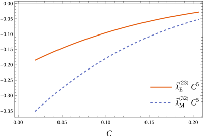
Figure 1: Electric-led and magnetic-led RTLNs for a static fluid with polytropic EoS with $n=1$. These results are obtained after correcting the numerical implementation of Paper I.

II.3 Static and irrotational relativistic TLNs

In Paper I it was assumed that the fluid is static, i.e. $\delta u^{i}=0$. More recently, it was found that the appropriate stationary limit of a time-dependent compact star has an irrotational fluid Landry and Poisson (2015a), in which $\delta g_{\mu\nu,0}=0$ as for static perturbations, but $\delta u^{i}$ can have an azimuthal component. In the irrotational case, the perturbation of the vorticity tensor,

$$\omega_{\alpha\beta}=\nabla_{\alpha}(hu_{\beta})-\nabla_{\beta}(hu_{\alpha})\,,$$ (31)

(with $h=(\rho+P)/n$, $n$ baryonic number density) identically vanishes. Conversely the static fluid, although mathematically consistent (it is an admissible solution of the field equations), cannot be retrieved as the static limit of a time-dependent solution, and thus should not be considered as physically sound.

For a non-rotating NS the irrotationality condition simply reduces to the vanishing of the covariant velocity perturbation, $\delta u_{i}=0$ Landry and Poisson (2015a); Pani et al. (2018), leading to $\delta u^{\phi}\propto\delta g_{t\phi}$. As discussed in Ref. Pani et al. (2018), this choice corresponds to the magnetic TLNs computed by Damour and Nagar Damour and Nagar (2009). For a rotating star the irrotational condition is much more involved, it does not reduce to a simple condition on the four-velocity components (see e.g. Lockitch et al. (2001)).

As noted in Gupta et al. (2020), this characterization of static and irrotational fluid configurations can be easily rephrased in a Lagrangian framework. If the internal Lagrangian does not depend on time, its variations yield the static perturbations. The irrotational perturbations, instead, are the zero-frequency limit of the equations obtained from a time-dependent Lagrangian.

In Paper II it was assumed that the Lagrangian ${\cal L}_{\rm int}$, describing the internal degrees of freedom of the star, depends on the multipole moments but not on their time derivatives: ${\cal L}_{\rm int}={\cal L}_{\rm int}(Q^{L}_{A},S^{L}_{A})$, see Eq. (26). Therefore, the adiabatic equations (24), arising from the variations $\partial{\cal L}/\partial Q^{L}_{A}$ and $\partial{\cal L}/\partial S^{L}_{A}$, correspond to static perturbations. Thus, the hidden symmetry (29)-(30) refers to static perturbations as well. In order to extend the results of Paper II to irrotational perturbations, we should consider an internal Lagrangian which depends (like the orbital Lagrangian) to ${\dot{Q}}^{L}_{A},{\dot{S}}^{L}_{A}$ as well, compute the variations with respect to the multipole moments, and finally consider the zero-frequency limit; we leave this computation for future work Castro et al. (2021).

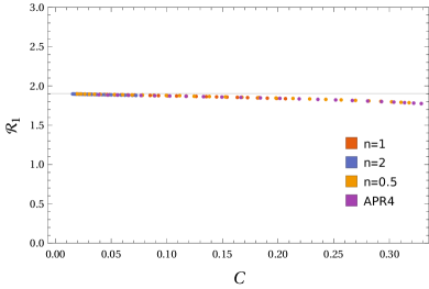
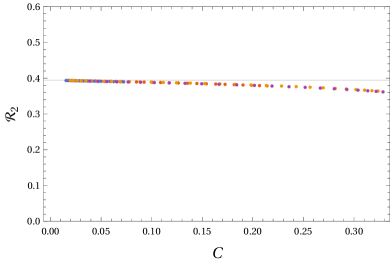
Figure 2: Ratios of RTLNs ${\cal R}_{1}$ (left panel) and ${\cal R}_{2}$ (right panel) [see Eq. (43)] as a function of the compactness $C$, for a polytropic EoS with $n=0.5$, $n=1$, $n=2$ and for the APR4 EoS. The horizontal line denotes the theoretical prediction from the Lagrangian formulation [Eq. (43)].

III Hidden symmetry of the RTLNs

We shall now explicitly compute the static RTLNs for different EoSs. We shall then verify whether the relations (29), (30) are satisfied.

III.1 Computation of the static RTLNs

In order to compute the magnetic RTLNs (17)

$$\lambda_{M}^{(ll^{\prime})}=\frac{\partial J_{l}}{\partial{\cal E}^{(l^{\prime})}_{0}}$$ (32)

with $l^{\prime}=l\pm 1$, and the rescaled quantities ${\tilde{\lambda}}_{M}^{(ll^{\prime})}=\lambda_{M}^{(ll^{\prime})}/(M^{l+l^{\prime}+1}\chi)$, we have to determine the current multipole perturbations $J_{l}$ induced by an electric tidal field ${\cal E}^{(l^{\prime})}_{0}$ (15); thus, we have to find the axial parity perturbations $h^{l}_{0}$ induced by polar parity perturbations $H_{0}^{l^{\prime}}$, by solving the polar-led equations (11). For ${\tilde{\lambda}}^{(23)}_{M}$, we have to consider the perturbations $h_{0}^{2}$ induced by $H_{0}^{3}$, and Eqs. (11) reduce to

$${\cal D}^{{\rm pol}\,(3)}[H_{0}^{3}] =0$$ (33)

$${\cal D}^{{\rm ax}\,(2)}[h_{0}^{2}] =S_{+}^{{\rm pol}\,(3)}[H_{0}^{3}]\,,$$ (34)

while for ${\tilde{\lambda}}^{(32)}_{M}$, we have to consider the perturbations $h_{0}^{3}$ induced by $H_{0}^{2}$, and Eqs. (11) reduce to

$${\cal D}^{{\rm pol}\,(2)}[H_{0}^{2}] =0$$ (35)

$${\cal D}^{{\rm ax}\,(3)}[h_{0}^{3}] =S_{+}^{{\rm pol}\,(2)}[H_{0}^{2}]\,.$$ (36)

Similarly, to compute the electric RTLNs (17)

$$\lambda_{E}^{(ll^{\prime})}=\frac{\partial M_{l}}{\partial{\cal B}^{(l^{\prime})}_{0}}$$ (37)

with $l^{\prime}=l\pm 1$, and the rescaled quantities ${\tilde{\lambda}}_{E}^{(ll^{\prime})}=\lambda_{E}^{(ll^{\prime})}/(M^{l+l^{\prime}+1}\chi)$, we have to determine the mass multipole perturbations $M_{l}$ induced by a magnetic tidal field ${\cal B}^{(l^{\prime})}_{0}$ (15). Thus, we have to find the polar parity perturbations $H^{l}_{0}$ induced by axial parity perturbations $h_{0}^{l^{\prime}}$, by solving the axial-led equation (14). For ${\tilde{\lambda}}^{(23)}_{E}$, we have to consider the perturbations $H_{0}^{2}$ induced by $h_{0}^{3}$, and Eqs. (14) reduce to

$${\cal D}^{{\rm ax}\,(3)}[h_{0}^{3}] =0$$ (38)

$${\cal D}^{{\rm pol}\,(2)}[H_{0}^{2}] =S_{+}^{{\rm ax}\,(3)}[h_{0}^{3}]\,,$$ (39)

while for ${\\ tildelambda}^{(32)}_{E}$, we have to consider the perturbations $H_{0}^{3}$ induced by $h_{0}^{2}$, and Eqs. (14) reduce to

$${\cal D}^{{\rm ax}\,(3)}[h_{0}^{2}] =0$$ (40)

$${\cal D}^{{\rm pol}\,(3)}[H_{0}^{3}] =S_{+}^{{\rm ax}\,(2)}[h_{0}^{2}]\,.$$ (41)

The explicit form of Eqs. (36)-(41) is given in Eqs. (12), (13) and in Appendix A.

For concreteness, let us consider a quadrupolar electric tidal perturbation, $\mathcal{E}_{0}^{(2)}$ (the computation of other multipoles follows straightforwardly). In practice, we start by solving Eq. (35) and then use its solution to source Eq. (36). Outside the star, we can solve the entire system analytically, obtaining a solution that satisfies the asymptotic behavior (15). The full treatment of the separation of the tidal and response parts of the solutions, as well as the definition of the solutions’ free constants, is the same as in Paper I.

The interior solutions have to be computed numerically. We start by performing an asymptotic expansion of Eq. (35) at $r=0$ to obtain the initial conditions (up to an overall constant) and integrate up to the radius of the star. We then match the two (interior and exterior) solutions and their first radial derivatives at the radius $R$, obtaining values for the free constants of the exterior solution (specifically, $\gamma_{2}$ and $\alpha_{2}$ as defined in Paper I) with which we compute the ($l=2$, electric) TLN of the non-spinning star, ${\tilde{\lambda}}_{E}^{(2)}$. Solving Eq. (36) follows a similar procedure, with the difference that – being an inhomogeneous equation – its full solution is obtained as a linear combination of a particular solution and the solution of the corresponding homogeneous equation. The arbitrary multiplicative factor in front of the homogeneous part – as well as the value of the free single constant of the exterior solution ($\gamma^{*}_{32}$ as defined in Paper I) – can be obtained via the matching at the radius of the star $R$. After this procedure one can simply extract the corresponding RTLN, ${\tilde{\lambda}}_{M}^{(32)}$.

We compute the electric and magnetic RTLNs with $l,l^{\prime}=2,3$ and $l,l^{\prime}=3,2$ for different values of the compactness $C=M/R$, for a sample of EoS consisting in the polytropic EoS with $n=0.5,1,2$ , and the APR4 EoS Akmal et al. (1998). The results of the computation (multiplied by $C^{6}$) are shown in Fig. 1. We stress that the computations presented here correct some errors in the numerical implementation of Paper I.

III.2 The hidden symmetry

Equations (29), (30) imply that the ratios of the RTLNs ${\tilde{\lambda}}^{(ll^{\prime})}_{E}$, ${\tilde{\lambda}}^{(ll^{\prime})}_{M}$ with $l,l^{\prime}=2,3$ and $l,l^{\prime}=3,2$, are constant

$${\cal R}_{1} \equiv\frac{{\tilde{\lambda}}^{(32)}_{M}}{{\tilde{\lambda}}^{(23)}_{E}}=\frac{9}{4}\sqrt{\frac{5}{7}}\simeq 1.902\,,$$ (42)

$${\cal R}_{2} \equiv\frac{{\tilde{\lambda}}^{(23)}_{M}}{{\tilde{\lambda}}^{(32)}_{E}}=\frac{1}{3}\sqrt{\frac{7}{5}}\simeq 0.394\,,$$ (43)

regardless of the NS mass and of the EoS. In Fig. (2) we show the ratios ${\cal R}_{1}$, ${\cal R}_{2}$ as functions of the compactness, for the sample of EoS considered in this paper (polytropic EoS with $n=0.5,1,2$ and APR4 EoS), together with the theoretical prediction (43).

Note that the theoretical prediction from the Lagrangian PN approach [Eq. (43)] is precisely satisfied in the small-compactness limit. When $C\lesssim 0.1$, the ratios ${\cal R}_{1}$, ${\cal R}_{2}$ coincide with the theoretical prediction within $1\%$, whereas for $C\sim 0.2-0.3$, the discrepancy increases (approximately) quadratically in $C$ up to $\sim 6\%$. We have verified that this discrepancy is significantly larger than the numerical errors, so it does not look as a numerical artifact. Moreover, for any compactness the ratios ${\cal R}_{1}$, ${\cal R}_{2}$ are independent on the EoS within $0.2\%$ (i.e., within the numerical error).

IV Discussion

Our results imply that a hidden symmetry among the static RTLNs with opposite parity actually exists, as suggested by the PN Lagrangian formulation of Paper I. This symmetry is exaclty satisfied in the small-compactness limit, and is therefore stronger than other approximately EoS-independent relations between the (spin- and tidal- induced) multipole moments of a NS Yagi and Yunes (2017). For large values of the compactness the hidden symmetry is weakly violated, but an EoS-independent (within numerical errors) relation is still present.

The very existence of this hidden symmetry is highly nontrivial and deserves further studies. In particular, it is not clear which is its underlying reason. From a Lagrangian point of view it is natural to expect that opposite sectors are coupled to each other, since a single interaction term in the form of Eq. (1) gives rise to related coupling terms in the field equations for ${\cal A}$ and ${\cal P}$ which are both proportional to the single coupling constant $\alpha$. On the other hand, justifying the origin of this symmetry from a pertubation-theory point of view is challenging, since there is a priori no reason why perturbations belonging to opposite parity sectors should be related to each other. This symmetry is somehow reminiscent of the relation between axial and polar perturbations in Schwarzschild black holes found by Chandrasekhar Chandrasekhar (1985), although in this case it involves the matter sector as well.

Another point that deserves future investigation is the dependence on the compactness. The latter does not enter directly in the Lagrangian formulation of Paper II, being encoded in the (R)TLNs. Our results suggest instead that the prediction from the PN expansion is valid only for low-compactness objects, and it acquires small corrections at large compactness.

Finally, in agreement with the framework of Paper II, we have focused on static perturbations. We anyway expect that qualitatively similar (but quantitatively different) relations exist among the irrotational RTLNs. In order to extend our results to the more realistic, irrotational case, one should include time dependence (and, possibly, nonaxisymmetry) in the tidal field, both in the Lagrangian and in the perturbation-theory formulations. This interesting problem will be discussed in a future work Castro et al. (2021).

Appendix A Explicit form of the coefficients and the source in the RTLN equations

In this appendix we give the explicit form of the coefficients in the definition of the operators ${\cal D}^{{\rm pol}\,(l)}$, ${\cal D}^{{\rm ax}\,(l)}$ given in Eqs. (12), (13), and of the source terms appearing in Eqs. (11), (14). We have:

$$C_{1}^{{\rm pol}\,(l)} =\frac{e^{\lambda(r)}\left[4\pi r^{2}\big{(}P(r)-\rho(r)\big{)}+1\right]+1}{r}$$ (44)

$$C_{0}^{{\rm pol}\,(l)} =\frac{4\pi e^{\lambda(r)}(P(r)+\rho(r))}{\frac{dP}{d\rho}}$$ (45)

$$-\frac{\left(8\pi r^{2}P(r)+1\right)^{2}e^{2\lambda(r)}}{r^{2}}$$

$$-\frac{e^{\lambda(r)}\left[-4\pi r^{2}\big{(}13P(r)+5\rho(r)\big{)}+l^{2}+l-2\right]+1}{r^{2}}$$

$$C_{1}^{{\rm ax}\,(l)} =-4\pi re^{\lambda(r)}(P(r)+\rho(r))$$ (46)

$$C_{0}^{{\rm ax}\,(l)} =-\frac{e^{\lambda(r)}\left[8\pi r^{2}(P(r)+\rho(r))\right]}{r^{2}}$$

$$-\frac{e^{\lambda(r)}\left[l^{2}+l-2\right]+2}{r^{2}}\,,$$ (47)

and

$$S_{+}^{{\rm pol}\,(l)} = \frac{1}{({l}({l}+1)-2)\sqrt{4{l}({l}+2)+3}{c_{s}^{2}}(r-2{\cal M})^{2}}\left[\kappa\left(2-{l}({l}+1)\right)r^{3}(r-2{\cal M})(P+\rho)({\tilde{\omega}}+\Omega){H_{0}^{({l})}}\right.$$ (48)

$$\left.-{c_{s}^{2}}\left({H_{0}^{({l})}}\left(2r{\cal M}\left(-\kappa r^{2}\rho\left(\left(5{{l}({l}+1)}-22\right)\Omega+({l}(5{l}+9)-6){\tilde{\omega}}\right)-2\left({l}\left({{l}({l}+1)}-4\right)-2\right)(\Omega-{\tilde{\omega}})\right.\right.\right.\right.$$

$$\left.\left.\left.\left.+\kappa r^{2}P\left(\Omega\left(3{l}({l}+5)+32\kappa r^{2}\rho+14\right)+(14-{l}(13{l}+25)){\tilde{\omega}}\right)+24\kappa^{2}r^{4}\Omega P^{2}+8\kappa^{2}r^{4}\Omega\rho^{2}\right)\right.\right.\right.$$

$$\left.\left.\left.+r^{2}\left(\kappa r^{2}\Omega\left(\rho\left(5{{l}({l}+1)}+16\kappa r^{2}P\left(\kappa r^{2}P-1\right)-14\right)+P\left(4\kappa r^{2}P\left({l}({l}+3)+4\kappa r^{2}P-2\right)+({l}-3){l}-6\right)\right.\right.\right.\right.\right.$$

$$\left.\left.\left.\left.\left.-8\kappa r^{2}\rho^{2}\right)+{\tilde{\omega}}\left(\kappa r^{2}\left(P\left(-4\kappa{l}({l}+3)r^{2}P+{l}(9{l}+13)-14\right)+({l}(5{l}+9)-6)\rho\right)-2{l}({l}({l}+1)-2)\right)\right.\right.\right.\right.$$

$$\left.\left.\left.\left.+2{l}({l}({l}+1)-2)\Omega\right)+4{\cal M}^{2}\left((({l}-1){l}-4)(\Omega-{\tilde{\omega}})-4\kappa r^{2}\Omega(P+\rho)\right)\right)\right.\right.$$

$$\left.\left.+2r(r-2{\cal M}){H_{0}^{({l})}}^{\prime}\left(({l}({l}+1)-2)r({\tilde{\omega}}-\Omega)+{\cal M}\left(({l}(3{l}+5)-4)(\Omega-{\tilde{\omega}})+4\kappa r^{2}\Omega(P+\rho)\right)\right.\right.\right.$$

$$\left.\left.\left.+\kappa r^{3}P\left({l}({l}+3)(\Omega-{\tilde{\omega}})+4\kappa r^{2}\Omega\rho\right)+4\kappa^{2}r^{5}\Omega P^{2}\right)\right)\right]\,,$$

$$S_{-}^{{\rm pol}\,({l})} = \frac{1}{({l}({l}+1)-2)\sqrt{4{l}^{2}-1}{c_{s}^{2}}(r-2{\cal M})^{2}}\left[{c_{s}^{2}}\left(2r(r-2{\cal M}){H_{0}^{({l})}}^{\prime}\left({\cal M}\left(\left(3{{l}({l}+1)}-6\right)(\Omega-{\tilde{\omega}})+4\kappa r^{2}\Omega(P+\rho)\right)\right.\right.\right.$$ (49)

$$\left.\left.\left.+r\left(\kappa r^{2}P\left(\left({{l}({l}-1)}-2\right)(\Omega-{\tilde{\omega}})+4\kappa r^{2}\Omega\rho\right)-({l}({l}+1)-2)(\Omega-{\tilde{\omega}})+4\kappa^{2}r^{4}\Omega P^{2}\right)\right)\right.\right.$$

$$\left.\left.+{H_{0}^{({l})}}\left(4{\cal M}^{2}\left(\left({l}^{2}+3{l}-2\right)(\Omega-{\tilde{\omega}})-4\kappa r^{2}\Omega P-4\kappa r^{2}\Omega\rho\right)+2r{\cal M}\left(\kappa r^{2}P\left(-\left(13{{l}({l}+1)}-26\right){\tilde{\omega}}\right.\right.\right.\right.\right.$$

$$\left.\left.\left.\left.\left.+\left(3{l}^{2}-9{l}+2\right)\Omega+32\kappa r^{2}\Omega\rho\right)-\kappa r^{2}\rho\left(\left(5{{l}({l}+1)}-10\right){\tilde{\omega}}+\left(5{l}^{2}+9{l}-18\right)\Omega\right)\right.\right.\right.\right.$$

$$\left.\left.\left.\left.+2\left({l}^{3}+2{l}^{2}-3{l}-2\right)(\Omega-{\tilde{\omega}})+24\kappa^{2}r^{4}\Omega P^{2}+8\kappa^{2}r^{4}\Omega\rho^{2}\right)+r^{2}\left(\kappa r^{2}P\left(\left(9{l}^{2}+5{l}-18\right){\tilde{\omega}}\right.\right.\right.\right.\right.$$

$$\left.\left.\left.\left.\left.+\left({l}^{2}+5{l}-2\right)\Omega-16\kappa r^{2}\Omega\rho\right)+4\kappa^{2}r^{4}P^{2}\left(\left(-{{l}({l}+1)}+2\right){\tilde{\omega}}+\left({{l}({l}-1)}-4\right)\Omega+4\kappa r^{2}\Omega\rho\right)\right.\right.\right.\right.$$

$$\left.\left.\left.\left.+\kappa r^{2}\rho\left(\left(5{{l}({l}+1)}-10\right){\tilde{\omega}}+\left(5{l}^{2}+9{l}-10\right)\Omega\right)-2\left({l}^{3}+2{{l}({l}-1)}-2\right)(\Omega-{\tilde{\omega}})+16\kappa^{3}r^{6}\Omega P^{3}-8\kappa^{2}r^{4}\Omega\rho^{2}\right)\right)\right)\right.$$

$$\left.+\kappa({l}({l}+1)-2)r^{3}(r-2{\cal M})(P+\rho)({\tilde{\omega}}+\Omega){H_{0}^{({l})}}\right]\,,$$

$$S_{+}^{{\rm ax}\,({l})} = \frac{2e^{-\nu}}{\sqrt{4{l}^{2}+8{l}+3}r^{2}{c_{s}^{2}}(r-2{\cal M})^{2}}\left[{c_{s}^{2}}\left(r(r-2{\cal M}){h_{0}^{({l})}}^{\prime}\left(-2{\cal M}\left(r{\tilde{\omega}}^{\prime}\left({{l}({l}+1)}+2\kappa r^{2}P+2\kappa r^{2}\rho+3\right)\right.\right.\right.\right.$$ (50)

$$\left.\left.\left.\left.+{\tilde{\omega}}\left(3{l}({l}+1)-4\kappa r^{2}P-4\kappa r^{2}\rho\right)-3{l}({l}+1)\Omega\right)+r\left(2\kappa r^{2}P\left({l}({l}+1)\Omega-{\tilde{\omega}}\left({{l}({l}+1)}-4\kappa r^{2}\rho\right)\right)+{l}^{2}r{\tilde{\omega}}^{\prime}\right.\right.\right.\right.$$

$$\left.\left.\left.\left.-2{l}^{2}\Omega+{l}r{\tilde{\omega}}^{\prime}+2{l}({l}+1){\tilde{\omega}}-2{l}\Omega-2\kappa^{2}r^{4}P^{2}\left(r{\tilde{\omega}}^{\prime}-4{\tilde{\omega}}\right)+2\kappa r^{3}\rho{\tilde{\omega}}^{\prime}\right)+10{\cal M}^{2}{\tilde{\omega}}^{\prime}\right)\right.\right.$$

$$\left.\left.+{h_{0}^{({l})}}\left(r^{2}\left(\kappa r^{2}P\left(2{\tilde{\omega}}\left({{l}({l}+1)}+12\kappa r^{2}\rho\right)-2{\tilde{\omega}}^{\prime}\left({l}r-4\kappa r^{3}\rho+r\right)-5{l}({l}+1)\Omega\right)+\kappa r^{2}\rho\left(2{l}({l}+1){\tilde{\omega}}\right.\right.\right.\right.\right.$$

$$\left.\left.\left.\left.\left.-5{l}({l}+1)\Omega-4r{\tilde{\omega}}^{\prime}\right)+2{l}({l}+1)^{2}(\Omega-{\tilde{\omega}})-20\kappa^{3}r^{6}P^{3}{\tilde{\omega}}-4\kappa^{2}r^{4}P^{2}\left({\tilde{\omega}}\left(5\kappa r^{2}\rho-4\right)-3r{\tilde{\omega}}^{\prime}\right)+8\kappa^{2}r^{4}\rho^{2}{\tilde{\omega}}\right)\right.\right.\right.$$

$$\left.\left.\left.-2r{\cal M}\left(-2{l}^{3}{\tilde{\omega}}+2{l}^{3}\Omega+\kappa r^{2}P\left(2{\tilde{\omega}}\left({{l}({l}+1)}+22\kappa r^{2}\rho+2\right)+2r{\tilde{\omega}}^{\prime}\left(4\kappa r^{2}\rho-5-{l}\right)-5{l}({l}+1)\Omega\right)\right.\right.\right.\right.$$

$$\left.\left.\left.\left.+\kappa r^{2}\rho\left(2\left({{l}({l}+1)}+2\right){\tilde{\omega}}-5{l}({l}+1)\Omega-12r{\tilde{\omega}}^{\prime}\right)-2{l}^{2}{\tilde{\omega}}+2{l}^{2}\Omega+{l}r{\tilde{\omega}}^{\prime}+12\kappa^{2}r^{4}P^{2}\left(r{\tilde{\omega}}^{\prime}+3{\tilde{\omega}}\right)\right.\right.\right.\right.$$

$$\left.\left.\left.\left.+8\kappa^{2}r^{4}\rho^{2}{\tilde{\omega}}-5r{\tilde{\omega}}^{\prime}\right)-4{\cal M}^{2}\left(r{\tilde{\omega}}^{\prime}\left(-{l}+8\kappa r^{2}P+8\kappa r^{2}\rho+10\right)+{\tilde{\omega}}\left(-2{l}({l}+1)+\kappa r^{2}P+\kappa r^{2}\rho\right)+2{l}({l}+1)\Omega\right)\right.\right.\right.$$

$$\left.\left.\left.+40{\cal M}^{3}{\tilde{\omega}}^{\prime}\right)\right)-\kappa r^{2}(P+\rho){h_{0}^{({l})}}\left(-2r{\cal M}\left({l}({l}+1)\Omega-4\kappa r^{2}P{\tilde{\omega}}\right)+r^{2}\left({l}({l}+1)\Omega+4\kappa^{2}r^{4}P^{2}{\tilde{\omega}}\right)+4{\cal M}^{2}{\tilde{\omega}}\right)\right]\,,$$

$$S_{-}^{{\rm ax}\,({l})} = \frac{2e^{-\nu}}{\sqrt{4{l}^{2}-1}r^{2}{c_{s}^{2}}(r-2{\cal M})^{2}}\left[{c_{s}^{2}}\left({h_{0}^{({l})}}\left(r^{2}\left(-\kappa r^{2}P\left(2{\tilde{\omega}}\left({{l}({l}+1)}+12\kappa r^{2}\rho\right)+2r{\tilde{\omega}}^{\prime}\left({l}+4\kappa r^{2}\rho\right)-5{l}({l}+1)\Omega\right)\right.\right.\right.\right.$$ (51)

$$\left.\left.\left.\left.+2{l}^{2}({l}+1)(\Omega-{\tilde{\omega}})+\kappa r^{2}\rho\left(-2{l}({l}+1){\tilde{\omega}}+5{l}({l}+1)\Omega+4r{\tilde{\omega}}^{\prime}\right)+20\kappa^{3}r^{6}P^{3}{\tilde{\omega}}\right.\right.\right.\right.$$

$$\left.\left.\left.\left.+4\kappa^{2}r^{4}P^{2}\left({\tilde{\omega}}\left(5\kappa r^{2}\rho-4\right)-3r{\tilde{\omega}}^{\prime}\right)-8\kappa^{2}r^{4}\rho^{2}{\tilde{\omega}}\right)+2r{\cal M}\left(2{l}^{3}{\tilde{\omega}}-2{l}^{3}\Omega+\kappa r^{2}P\left(2{\tilde{\omega}}\left({{l}({l}+1)}+22\kappa r^{2}\rho+2\right)\right.\right.\right.\right.\right.$$

$$\left.\left.\left.\left.\left.+2r{\tilde{\omega}}^{\prime}\left({l}+4\kappa r^{2}\rho-4\right)-5{l}({l}+1)\Omega\right)+\kappa r^{2}\rho\left(2\left({{l}({l}+1)}+2\right){\tilde{\omega}}-5{l}({l}+1)\Omega-12r{\tilde{\omega}}^{\prime}\right)+4{l}^{2}(\tilde{\omega}-\Omega)\right.\right.\right.\right.$$

$$\left.\left.\left.\left.-{l}r{\tilde{\omega}}^{\prime}+2{l}{\tilde{\omega}}-2{l}\Omega+12\kappa^{2}r^{4}P^{2}\left(r{\tilde{\omega}}^{\prime}+3{\tilde{\omega}}\right)+8\kappa^{2}r^{4}\rho^{2}{\tilde{\omega}}-6r{\tilde{\omega}}^{\prime}\right)+4{\cal M}^{2}\left(r{\tilde{\omega}}^{\prime}\left({l}+8\kappa r^{2}P+8\kappa r^{2}\rho+11\right)\right.\right.\right.\right.$$

$$\left.\left.\left.\left.+{\tilde{\omega}}\left(-2{l}({l}+1)+\kappa r^{2}P+\kappa r^{2}\rho\right)+2{l}({l}+1)\Omega\right)-40{\cal M}^{3}{\tilde{\omega}}^{\prime}\right)-r(r-2{\cal M}){h_{0}^{({l})}}^{\prime}\left(-2{\cal M}\left(r{\tilde{\omega}}^{\prime}\left({{l}({l}+1)}\right.\right.\right.\right.\right.$$

$$\left.\left.\left.\left.\left.+2\kappa r^{2}(P+\rho)+3\right)+{\tilde{\omega}}\left(3{l}({l}+1)-4\kappa r^{2}P-4\kappa r^{2}\rho\right)-3{l}({l}+1)\Omega\right)\right.\right.\right.$$

$$\left.\left.\left.+r\left(2\kappa r^{2}P\left({l}({l}+1)\Omega-{\tilde{\omega}}\left({{l}({l}+1)}-4\kappa r^{2}\rho\right)\right)+{l}^{2}r{\tilde{\omega}}^{\prime}-2{l}^{2}\Omega+{l}r{\tilde{\omega}}^{\prime}+2{l}({l}+1){\tilde{\omega}}-2{l}\Omega\right.\right.\right.\right.$$

$$\left.\left.\left.\left.-2\kappa^{2}r^{4}P^{2}\left(r{\tilde{\omega}}^{\prime}-4{\tilde{\omega}}\right)+2\kappa r^{3}\rho{\tilde{\omega}}^{\prime}\right)+10{\cal M}^{2}\tilde{\omega}^{\prime}\right)\right)+\kappa r^{2}(P+\rho){h_{0}^{({l})}}\left(-2r{\cal M}\left({l}({l}+1)\Omega-4\kappa r^{2}P{\tilde{\omega}}\right)\right.\right.$$

$$\left.\left.+r^{2}\left({l}({l}+1)\Omega+4\kappa^{2}r^{4}P^{2}{\tilde{\omega}}\right)+4{\cal M}^{2}{\tilde{\omega}}\right)\right]\,,$$

where $\kappa=4\pi$ and $c_{s}=\sqrt{dP/d\rho}$ is the sound speed in the fluid.

Appendix B Comparison between different conventions for the (R)TLNs

We shall compare the definitions and notations of TLNs and RTLNs in Paper I and in Paper II, in order to find the rescaling factors appearing in Eq. (25). For the reader’s convenience, we repeat here some of the relations that appear in the main text, so that the derivation is self-contained.

In Paper I the adiabatic relations among multipole moments read [see Eq. (19)],

$$\frac{M_{2}}{M^{3}} =\tilde{\lambda}^{(2)}_{E}{\cal E}^{(2)}_{0}M^{2}+\chi\tilde{\lambda}^{(23)}_{E}{\cal B}_{0}^{(3)}M^{3}$$

$$\frac{M_{3}}{M^{4}} =\tilde{\lambda}^{(3)}_{E}{\cal E}^{(3)}_{0}M^{3}+\chi\tilde{\lambda}^{(32)}_{E}{\cal B}_{0}^{(2)}M^{2}$$

$$\frac{J_{2}}{M^{3}} =\tilde{\lambda}^{(2)}_{M}{\cal B}^{(2)}_{0}M^{2}+\chi\tilde{\lambda}^{(23)}_{M}{\cal E}_{0}^{(3)}M^{3}$$

$$\frac{J_{3}}{M^{4}} =\tilde{\lambda}^{(3)}_{M}{\cal B}^{(3)}_{0}M^{3}+\chi\tilde{\lambda}^{(32)}_{M}{\cal E}_{0}^{(2)}M^{2}\,,$$ (52)

where $M_{l}$, $J_{l}$ are the Geroch-Hansen multipole moments and ${\cal E}^{(l)}_{0}$, ${\cal B}_{0}^{(l)}$ are the tidal tensor components defined from the asymptotic limit of the metric in Eq. (15). Conversely, in Paper II they read (24) (in $c=1$ units)

$$Q^{ab} =\lambda_{2}G^{ab}+\lambda_{23}J^{c}H^{abc}\,,$$

$$Q^{abc} =\lambda_{3}G^{abc}+\lambda_{32}J^{<c}H^{ab>}\,,$$

$$S^{ab} =\sigma_{2}H^{ab}+\sigma_{23}J^{c}G^{abc}\,,$$

$$S^{abc} =\sigma_{3}H^{abc}+\sigma_{32}J^{<c}G^{ab>}\,,$$ (53)

where $Q^{L}$, $S^{L}$ are Thorne’s multipole moments, and $G^{L}$, $H^{L}$ are the tidal tensor components, defined (in spherical harmonic notation) from the asymptotic limit expansion (23). In order to express Eqs. (53) in terms of spherical harmonics components, we note that (see Sec. (I.1))

$$Q^{ab} =\sum_{m}Q^{2m}{\cal Y}^{2m}_{ab}=Q^{20}{\cal Y}^{20}_{ab}$$

$$Q^{abc} =\sum_{m}Q^{2m}{\cal Y}^{3m}_{abc}=Q^{30}{\cal Y}^{30}_{abc}$$ (54)

where we have assumed axisymmetry; the same applies to the current multipole moments $S^{ab}$, $S^{abc}$ and to the tidal tensor components. Moreover, $J^{a}=\chi k^{a}M^{2}$. Therefore,

$$Q^{20}{\cal Y}^{20}_{ab} =\lambda_{2}G^{20}{\cal Y}^{20}_{ab}+\lambda_{23}\chi M^{2}H^{30}{\cal Y}^{30}_{abc}k^{c}$$

$$Q^{30}{\cal Y}^{30}_{abc} =\lambda_{3}G^{30}{\cal Y}^{30}_{abc}+\lambda_{32}\chi M^{2}H^{20}{\cal Y}^{20}_{<ab}k_{c>}$$

$$S^{20}{\cal Y}^{20}_{ab} =\sigma_{2}H^{20}{\cal Y}^{20}_{ab}+\sigma_{23}\chi M^{2}G^{30}{\cal Y}^{30}_{abc}k^{c}$$

$$S^{30}{\cal Y}^{30}_{abc} =\sigma_{3}H^{30}{\cal Y}^{30}_{abc}+\sigma_{32}\chi M^{2}G^{20}{\cal Y}^{20}_{<ab}k_{c>}\,.$$ (55)

Since ${\cal Y}^{lm}_{ab}{\cal Y}^{*lm^{\prime}}_{ab}=N_{l}^{-1}\delta^{mm^{\prime}}$ with $N_{l}=4\pi l!/(2l+1)!!$, we find

$$Q^{20} =\lambda_{2}G^{20}+\lambda_{23}\chi M^{2}H^{30}KN_{2}$$

$$Q^{30} =\lambda_{3}G^{30}+\lambda_{32}\chi M^{2}H^{20}KN_{3}$$

$$S^{20} =\sigma_{2}H^{20}+\sigma_{23}\chi M^{2}G^{30}KN_{2}$$

$$S^{30} =\sigma_{3}H^{30}+\sigma_{32}\chi M^{2}G^{20}KN_{3}\,.$$ (56)

where we defined $K={\cal Y}^{30}_{abc}k^{c}{\cal Y}^{*20}_{ab}$. Since Poisson and Will (2014a) ${\cal Y}^{20}_{ab}=-\sqrt{5/(16\pi)}\delta_{ab}$ and ${\cal Y}^{30}_{abc}k^{c}=\sqrt{7/(16\pi)}\delta_{ab}$,

$$K=\frac{3}{16\pi}\sqrt{35}\,.$$ (57)

The Thorne multipole moments are related to the Geroch-Hansen multipole moments by Eq. (4),

$$Q^{i_{1}\cdots i_{l}}=M_{l}k^{i_{1}\cdots i_{l}}~{}~{},~{}~{}~{}~{}~{}S^{i_{1}\cdots i_{l}}=\frac{l+1}{2l}J_{l}k^{i_{1}\cdots i_{l}}\,,$$ (58)

thus, since (see Sec. (I.1)) $Q^{i_{1}\cdots i_{l}}n_{i_{1}\cdots i_{l}}=\sum_{m}Q^{lm}Y^{lm}=Q^{l0}Y^{l0}$ and the same applies to $S^{i_{1}\cdots i_{l}}$,

$$M_{l}k^{i_{1}\cdots i_{l}}n_{i_{1}\cdots i_{l}} =\sqrt{\frac{2l+1}{4\pi}}Q^{l0}P_{l}(\cos\theta)$$

$$\frac{l+1}{2l}J_{l}k^{i_{1}\cdots i_{l}}n_{i_{1}\cdots i_{l}} =\sqrt{\frac{2l+1}{4\pi}}S^{l0}P_{l}(\cos\theta)\,,$$ (59)

where $P_{l}$ are the Legendre polynomials. Then, since Poisson and Will (2014a) $k^{i_{1}\cdots i_{l}}n_{i_{1}\cdots i_{l}}=l!/(2l-1)!!P_{l}(\cos\theta)$,

$$Q^{l0} =\frac{l!}{(2l-1)!!}\sqrt{\frac{4\pi}{2l+1}}M_{l}$$

$$S^{l0} =\frac{(l+1)!}{2l(2l-1)!!}\sqrt{\frac{4\pi}{2l+1}}J_{l}\,.$$ (60)

Moreover, by comparing Eqs. (15), (23) we find that the tidal tensor components in the notations of Paper I and of Paper II are related by

$$G^{lm} =-(l-2)!{\cal E}_{m}^{(l)}$$

$$H^{lm} =-\frac{2}{3}(l+1)(l-2)!{\cal B}_{m}^{(l)}\,.$$ (61)

By replacing Eqs. (60), (61) in Eq. (56) we find

$$M_{2} =-\frac{3}{2}\sqrt{\frac{5}{4\pi}}\lambda_{2}{\cal E}_{0}^{(2)}-\frac{32\pi}{15}\sqrt{\frac{5}{4\pi}}\chi M^{2}K\lambda_{23}{\cal B}_{0}^{(3)}$$

$$M_{3} =-\frac{5}{2}\sqrt{\frac{7}{4\pi}}\lambda_{3}{\cal E}_{0}^{(3)}-\frac{8\pi}{7}\sqrt{\frac{7}{4\pi}}\chi M^{2}K\lambda_{32}{\cal B}_{0}^{(2)}$$

$$J_{2} =-4\sqrt{\frac{5}{4\pi}}\sigma_{2}{\cal B}_{0}^{(2)}-\frac{16\pi}{15}\sqrt{\frac{5}{4\pi}}\chi M^{2}K\sigma_{23}{\cal E}_{0}^{(3)}$$

$$J_{3} =-10\sqrt{\frac{7}{4\pi}}\sigma_{3}{\cal B}_{0}^{(3)}-\frac{6\pi}{7}\sqrt{\frac{5}{4\pi}}\chi M^{2}K\sigma_{32}{\cal E}_{0}^{(2)}\,.$$ (62)

By comparing with Eq. (52) and replacing Eq. (57), we finally obtain Eqs. (25), i.e. the relation between TLNs and RTLNs in the notations of Paper I and Paper II.

References

- Murray and Dermott (2000) C. Murray and S. Dermott, Solar System Dynamics (Cambridge University Press, Cambridge, UK, 2000).
- Poisson and Will (2014a) E. Poisson and C. M. Will, Gravity: Newtonian, Post-Newtonian, Relativistic (Cambridge University Press, 2014).
- Baiotti et al. (2010) L. Baiotti, T. Damour, B. Giacomazzo, A. Nagar, and L. Rezzolla, Phys.Rev.Lett. 105, 261101 (2010), arXiv:1009.0521 [gr-qc] .
- Baiotti et al. (2011) L. Baiotti, T. Damour, B. Giacomazzo, A. Nagar, and L. Rezzolla, Phys.Rev. D84, 024017 (2011), arXiv:1103.3874 [gr-qc] .
- Vines et al. (2011) J. Vines, E. E. Flanagan, and T. Hinderer, Phys. Rev. D83, 084051 (2011), arXiv:1101.1673 [gr-qc] .
- Pannarale et al. (2011) F. Pannarale, L. Rezzolla, F. Ohme, and J. S. Read, Phys.Rev. D84, 104017 (2011), arXiv:1103.3526 [astro-ph.HE] .
- Vines and Flanagan (2013) J. E. Vines and E. E. Flanagan, Phys. Rev. D88, 024046 (2013), arXiv:1009.4919 [gr-qc] .
- Lackey et al. (2012) B. D. Lackey, K. Kyutoku, M. Shibata, P. R. Brady, and J. L. Friedman, Phys.Rev. D85, 044061 (2012), arXiv:1109.3402 [astro-ph.HE] .
- Lackey et al. (2014) B. D. Lackey, K. Kyutoku, M. Shibata, P. R. Brady, and J. L. Friedman, Phys.Rev. D89, 043009 (2014), arXiv:1303.6298 [gr-qc] .
- Favata (2014) M. Favata, Phys.Rev.Lett. 112, 101101 (2014), arXiv:1310.8288 [gr-qc] .
- Yagi and Yunes (2014) K. Yagi and N. Yunes, Phys.Rev. D89, 021303 (2014), arXiv:1310.8358 [gr-qc] .
- Maselli et al. (2013a) A. Maselli, V. Cardoso, V. Ferrari, L. Gualtieri, and P. Pani, Phys. Rev. D88, 023007 (2013a), arXiv:1304.2052 [gr-qc] .
- Maselli et al. (2013b) A. Maselli, L. Gualtieri, and V. Ferrari, Phys.Rev. D88, 104040 (2013b), arXiv:1310.5381 [gr-qc] .
- Del Pozzo et al. (2013) W. Del Pozzo, T. G. F. Li, M. Agathos, C. Van Den Broeck, and S. Vitale, Phys. Rev. Lett. 111, 071101 (2013), arXiv:1307.8338 [gr-qc] .
- Abbott et al. (2017) B. Abbott et al. (Virgo, LIGO Scientific), Phys. Rev. Lett. 119, 161101 (2017), arXiv:1710.05832 [gr-qc] .
- Bauswein et al. (2017) A. Bauswein, O. Just, H.-T. Janka, and N. Stergioulas, Astrophys. J. 850, L34 (2017), arXiv:1710.06843 [astro-ph.HE] .
- Most et al. (2018) E. R. Most, L. R. Weih, L. Rezzolla, and J. Schaffner-Bielich, (2018), arXiv:1803.00549 [gr-qc] .
- Harry and Hinderer (2018) I. Harry and T. Hinderer, (2018), arXiv:1801.09972 [gr-qc] .
- Annala et al. (2017) E. Annala, T. Gorda, A. Kurkela, and A. Vuorinen, (2017), arXiv:1711.02644 [astro-ph.HE] .
- De et al. (2018) S. De, D. Finstad, J. M. Lattimer, D. A. Brown, E. Berger, and C. M. Biwer, (2018), arXiv:1804.08583 [astro-ph.HE] .
- Akcay et al. (2019) S. Akcay, S. Bernuzzi, F. Messina, A. Nagar, N. Ortiz, and P. Rettegno, Phys. Rev. D 99, 044051 (2019), arXiv:1812.02744 [gr-qc] .
- Guerra Chaves and Hinderer (2019) A. Guerra Chaves and T. Hinderer, J. Phys. G 46, 123002 (2019), arXiv:1912.01461 [nucl-th] .
- Chatziioannou (2020) K. Chatziioannou, (2020), arXiv:2006.03168 [gr-qc] .
- Yagi and Yunes (2013a) K. Yagi and N. Yunes, Phys. Rev. D88, 023009 (2013a), arXiv:1303.1528 [gr-qc] .
- Yagi and Yunes (2013b) K. Yagi and N. Yunes, Science 341, 365 (2013b), arXiv:1302.4499 [gr-qc] .
- Yagi and Yunes (2017) K. Yagi and N. Yunes, Phys. Rept. 681, 1 (2017), arXiv:1608.02582 [gr-qc] .
- Cardoso et al. (2017) V. Cardoso, E. Franzin, A. Maselli, P. Pani, and G. Raposo, Phys. Rev. D95, 084014 (2017), [Addendum: Phys. Rev.D95,no.8,089901(2017)], arXiv:1701.01116 [gr-qc] .
- Pani and Maselli (2019) P. Pani and A. Maselli, Int. J. Mod. Phys. D 28, 1944001 (2019), arXiv:1905.03947 [gr-qc] .
- Cardoso and Pani (2019) V. Cardoso and P. Pani, Living Rev. Rel. 22, 4 (2019), arXiv:1904.05363 [gr-qc] .
- Abbott et al. (2020) B. Abbott et al. (LIGO Scientific, Virgo), Astrophys. J. Lett. 892, L3 (2020), arXiv:2001.01761 [astro-ph.HE] .
- Abdelsalhin et al. (2018) T. Abdelsalhin, L. Gualtieri, and P. Pani, Phys. Rev. D98, 104046 (2018), arXiv:1805.01487 [gr-qc] .
- Jimenez-Forteza et al. (2018) X. Jimenez-Forteza, T. Abdelsalhin, P. Pani, and L. Gualtieri, (2018), arXiv:1807.08016 [gr-qc] .
- Banihashemi and Vines (2018) B. Banihashemi and J. Vines, (2018), arXiv:1805.07266 [gr-qc] .
- Dietrich et al. (2019) T. Dietrich, A. Samajdar, S. Khan, N. K. Johnson-McDaniel, R. Dudi, and W. Tichy, Phys. Rev. D 100, 044003 (2019), arXiv:1905.06011 [gr-qc] .
- Dietrich et al. (2020) T. Dietrich, T. Hinderer, and A. Samajdar, (2020), arXiv:2004.02527 [gr-qc] .
- Henry et al. (2020) Q. Henry, G. Faye, and L. Blanchet, (2020), arXiv:2005.13367 [gr-qc] .
- Flanagan and Hinderer (2008) E. E. Flanagan and T. Hinderer, Phys. Rev. D77, 021502 (2008), arXiv:0709.1915 [astro-ph] .
- Hinderer (2008) T. Hinderer, Astrophys. J. 677, 1216 (2008), arXiv:0711.2420 [astro-ph] .
- Pani et al. (2018) P. Pani, L. Gualtieri, T. Abdelsalhin, and X. Jiménez-Forteza, Phys. Rev. D 98, 124023 (2018), arXiv:1810.01094 [gr-qc] .
- Poisson (2020a) E. Poisson, Phys. Rev. D 102, 064059 (2020a), arXiv:2007.01678 [gr-qc] .
- Landry and Poisson (2015a) P. Landry and E. Poisson, Phys. Rev. D91, 104026 (2015a), arXiv:1504.06606 [gr-qc] .
- Landry and Poisson (2015b) P. Landry and E. Poisson, Phys. Rev. D92, 124041 (2015b), arXiv:1510.09170 [gr-qc] .
- Pani et al. (2015a) P. Pani, L. Gualtieri, and V. Ferrari, Phys. Rev. D92, 124003 (2015a), arXiv:1509.02171 [gr-qc] .
- Landry and Poisson (2015c) P. Landry and E. Poisson, Phys. Rev. D91, 104018 (2015c), arXiv:1503.07366 [gr-qc] .
- Landry (2017) P. Landry, Phys. Rev. D95, 124058 (2017), arXiv:1703.08168 [gr-qc] .
- Gagnon-Bischoff et al. (2018) J. Gagnon-Bischoff, S. R. Green, P. Landry, and N. Ortiz, Phys. Rev. D97, 064042 (2018), arXiv:1711.05694 [gr-qc] .
- Poisson (2015) E. Poisson, Phys. Rev. D91, 044004 (2015), arXiv:1411.4711 [gr-qc] .
- Pani et al. (2015b) P. Pani, L. Gualtieri, A. Maselli, and V. Ferrari, Phys. Rev. D92, 024010 (2015b), arXiv:1503.07365 [gr-qc] .
- Binnington and Poisson (2009) T. Binnington and E. Poisson, Phys. Rev. D80, 084018 (2009), arXiv:0906.1366 [gr-qc] .
- Damour and Nagar (2009) T. Damour and A. Nagar, Phys. Rev. D80, 084035 (2009), arXiv:0906.0096 [gr-qc] .
- Damour and Lecian (2009) T. Damour and O. M. Lecian, Phys.Rev. D80, 044017 (2009), arXiv:0906.3003 [gr-qc] .
- Gürlebeck (2015) N. Gürlebeck, Phys. Rev. Lett. 114, 151102 (2015), arXiv:1503.03240 [gr-qc] .
- Porto (2016) R. A. Porto, Fortsch. Phys. 64, 723 (2016), arXiv:1606.08895 [gr-qc] .
- Hui et al. (2020) L. Hui, A. Joyce, R. Penco, L. Santoni, and A. R. Solomon, (2020), arXiv:2010.00593 [hep-th] .
- Charalambous et al. (2021) P. Charalambous, S. Dubovsky, and M. M. Ivanov, (2021), arXiv:2103.01234 [hep-th] .
- Le Tiec and Casals (2020) A. Le Tiec and M. Casals, (2020), arXiv:2007.00214 [gr-qc] .
- Chia (2020) H. S. Chia, (2020), arXiv:2010.07300 [gr-qc] .
- Hartle (1973) J. B. Hartle, Phys. Rev. D8, 1010 (1973).
- Hughes (2001) S. A. Hughes, Phys. Rev. D 64, 064004 (2001).
- Poisson (2020b) E. Poisson, (2020b), arXiv:2012.10184 [gr-qc] .
- Castro et al. (2021) G. Castro, P. Pani, and L. Gualtieri, (2021), Irrotational tidal Love numbers of spinning neutron stars (in preparation, 2021).
- Chandrasekhar (1985) S. Chandrasekhar, The mathematical theory of black holes (1985).
- Thorne (1980) K. S. Thorne, Rev. Mod. Phys. 52, 299 (1980).
- Poisson and Will (2014b) E. Poisson and C. M. Will, Gravity: Newtonian, post-newtonian, relativistic (Cambridge University Press, 2014).
- Geroch (1970) R. P. Geroch, J. Math. Phys. 11, 2580 (1970).
- Hansen (1974) R. O. Hansen, J. Math. Phys. 15, 46 (1974).
- Cardoso and Gualtieri (2016) V. Cardoso and L. Gualtieri, Class. Quant. Grav. 33, 174001 (2016), arXiv:1607.03133 [gr-qc] .
- Gürsel (1983) Y. Gürsel, General Relativity and Gravitation 15, 737 (1983).
- Ryan (1995) F. Ryan, Phys. Rev. D 52, 5707 (1995).
- Poisson and Doucot (2017) E. Poisson and J. Doucot, Phys. Rev. D95, 044023 (2017), arXiv:1612.04255 [gr-qc] .
- Hartle (1967) J. B. Hartle, Astrophys. J. 150, 1005 (1967).
- Thorne and Hartle (1984) K. S. Thorne and J. B. Hartle, Phys. Rev. D 31, 1815 (1984).
- Regge and Wheeler (1957) T. Regge and J. A. Wheeler, Phys. Rev. 108, 1063 (1957).
- Thorne (1998) K. S. Thorne, Phys. Rev. D 58, 124031 (1998), arXiv:gr-qc/9706057 .
- Pani (2013) P. Pani, International Journal of Modern Physics A 28, 1340018 (2013), https://doi.org/10.1142/S0217751X13400186 .
- Abdelsalhin (2019) T. Abdelsalhin, Tidal deformations of compact objects and gravitational wave emission, Ph.D. thesis, Sapienza University of Rome (2019), arXiv:1905.00408 [gr-qc] .
- Maselli et al. (2012) A. Maselli, L. Gualtieri, F. Pannarale, and V. Ferrari, Phys. Rev. D 86, 044032 (2012), arXiv:1205.7006 [gr-qc] .
- Steinhoff et al. (2016) J. Steinhoff, T. Hinderer, A. Buonanno, and A. Taracchini, Phys. Rev. D 94, 104028 (2016), arXiv:1608.01907 [gr-qc] .
- Lockitch et al. (2001) K. H. Lockitch, N. Andersson, and J. L. Friedman, Phys. Rev. D 63, 024019 (2001), arXiv:gr-qc/0008019 .
- Gupta et al. (2020) P. K. Gupta, J. Steinhoff, and T. Hinderer, (2020), arXiv:2011.03508 [gr-qc] .
- Akmal et al. (1998) A. Akmal, V. R. Pandharipande, and D. G. Ravenhall, Phys. Rev. C58, 1804 (1998), arXiv:nucl-th/9804027 [nucl-th] .