Department of Physics
\universityBen Gurion University of the Negev
\crest
\degreetitleDoctor of Philosophy
\subjectLaTeX
Numerical analysis of the Primordial Power Spectrum for inflationary potentials
Abstract
In this work we study small field models of inflation, which, against previous expectations, yield significant Gravitational Wave (GW) signal, while reproducing other measured observable quantities in the Cosmic Microwave Background (CMB). We numerically study these, using previously published analytic works as general guidelines. We first discuss the framework necessary to understand the model building procedure and some of its motivations. We review the slow-roll paradigm, derive the slow-roll parameters and discuss different formulations thereof. We further present the Lyth bound and its theoretical descendants and finally, we outline the small/large field taxonomy and their characterization in the current nomenclature.
We proceed to present our models and the methods used in their building and examination. We employ MCMC simulations to evaluate model likelihoods and by process of marginalization extract the most probable coefficients for these inflationary potentials. An additional method applied is a multinomial fit, where we create a functional correspondence between coefficients and observables. This allows us to use the observable values directly to yield the most likely coefficients. We compare the results of the two methods and evaluate the level of tuning required for these models.
We discuss an apparent discrepancy between analytical approaches of evaluating Primordial Power Spectrum (PPS) observables and the precise numerical results in our models. We identify some of the sources of this discrepancy and remark on their meaning in the age of precision cosmology.
Finally, we present the results of our study, for the most likely inflationary models with polynomial potentials of degree 5, and 6. We demonstrate our ability to produce potentials that yield GW with a tensor-to-scalar ratio . This is a realistic expectation of GW detection sensitivity in the near future. Detecting GW of a primordial source will provide a direct indication of the energy scale of inflation, and therefore an interesting probe into physics beyond the standard model.
keywords:
LaTeX PhD Thesis Engineering University of CambridgeFor Netta, Tamar, Meir and Daya.
I hereby declare that except where specific reference is made to the work of others, the contents of this dissertation are original and have not been submitted in whole or in part for consideration for any other degree or qualification in this, or any other university. This dissertation is my own work and contains nothing which is the outcome of work done in collaboration with others, except as specified in the text and Acknowledgements. This dissertation contains fewer than 65,000 words including appendices, bibliography, footnotes, tables and equations and has fewer than 150 figures.
Acknowledgements.
I want to acknowledge, first and foremost my advisor, Prof. Ramy Brustein, for taking a chance on a young student coming hat-in-hand to start working in the mostly barren field of numerical cosmology in Israel. As is the case oftentimes, professional disagreements were not hard to come by, but the personal and professional guidance was always available. Instrumental in my scietific coding ‘upbringing’ were Dr. Rahul "write your own" Kumar, and Dr. Daniel "you’re wrong" Ariad. These people were there when I was but a seedling of the computational physicist I am today, and I am forever in their debt.In the later stages of my doctoral adventure, several people were instrumental in guiding me or, at the very least, providing a sounding board for my craziness. Dr. Ido Ben-Dayan contributed time and effort to bring me up to speed in all matters of observational and experimental cosmology. Snir "Erdelyi" Cohen, Tomer "Deadpool" Ygael , and Yossi "Pigal" Naor were the usual victims of my (temporary, physics induced) insanity.
When PhD has grown terminal, two main people were instrumental in ‘bringing it all together’. Prof. Eiichiro Komatsu, who, with a 30-minute talk crystallized many insights, and sharpened them into a point-like focus of what it meant to be a physicist. And Dr. Yuval Ben-Abu, who never, not even for a minute, let me rest. He always pushed me towards the next great challenge.
There is still a long list of thanks due, which is in no way exhaustive:
Prof. Antonio Riotto, for his support and invaluable advice.
Members of my advisory committee, professors Eduardo Guendelman and Uri Keshet.
Sifu and Shermu, Donald and Cheryl-Lynn Rubbo.
And my family and friends, chief among them are my parents - Joshua and Pnina Wolfson.
In this as in everything I owe my life to my wife, Netta Schramm.
Chapter 1 Scientific Introduction - State of the art
Even from the infancy stages of humanity, the question of origins was an ever-present one. Every religion in existence and in fact, every culture, incorporates an origin story for the universe.
Up until the new era of scientific renaissance, this field was dominated predominantly by theologists, mystics and story-tellers. Some may attribute this to proper education being exclusive to members of the upper religious castes.
1.1 The evidence for a hot Big Bang
It is not until Einstein’s theory of relativity that we can construct an origin story of sufficient precision, to exclude divine intervention. At least a manifest one.
In the early 20th century, Alexander Friedmann, using Einstein’s own theory of relativity, was able to derive an equation of motion for the evolution of the universeFriedmannEqs; 1999GReGr..31.1991F . It took about seven years, Friedmann’s death, and Georges Lemaître’s independent work 1927ASSB...47...49L; 1931MNRAS..91..483L, for Einstein to accept the idea that his new physics proposed a mechanism for the evolution of the cosmos itself. Coupled with Edwin Hubble’s observations and the Hubble law HubbleLaw, this initiated a flood of scientific theories regarding the origin of our universe, with three main competing scenarios:
-
•
A static universe - Most famously connected to Einstein’s “biggest blunder", the cosmological constant Einstein:1917:KBA.
-
•
An ever expanding universe where matter is constantly created, to fill in the newly created space.
-
•
An evolving universe which is currently expanding, originated by a primordial explosion-like event.
The last of which was ridiculed by the pre-eminent cosmologist Fred Hoyle, who coined the then derogatory phrase “Big Bang theory" - in response to the notion of matter and energy created ex-nihilo at the onset of our universe, to give rise to rapid expansion.
This last “Big Bang theory", became the lead contender in 1965 when Arno Penzias and Robert Wilson, of Bell labs, stumbled upon the Cosmic Microwave Background Radiation (CMBR or CMB) Penzias_Wilson1965. Dicke, Peebles and Wilkinson, themselves working on a microwave band antenna at the time, were able to provide the theoretical framework that would explain this as a remnant of the “Big Bang" DickeWilkinsonPeebles1965. This, together with different mounting evidence of light-element abundance in the universe was sufficient confirmation of the “Big Bang" as the most probable physical scenario.
1.2 Problems with the old big bang model
Several measurements of the CMB temperature spectrum were made starting with Penzias and Wilson Penzias_Wilson1965, through Thaddeus Thaddeus:1972an and others, but the first overwhelming evidence of the black-body spectrum of the CMB was found by the Far-Infrared Absolute Spectrophotometer (FIRAS) instrument on the Cosmic Background Explorer (COBE) satellite Mather:1998gm. From these measurements, with systematic dominated error margins of no more than 0.3% at peak brightness, and an rms value of 0.01%. This extraordinary precision in measuring the black-body nature of the CMB put the "Big Bang theory" on as sound a footing as anyone could hope for. However, as with all scientific discoveries, one answer gives rise to a multitude of other problems.
1.2.1 The horizon problem
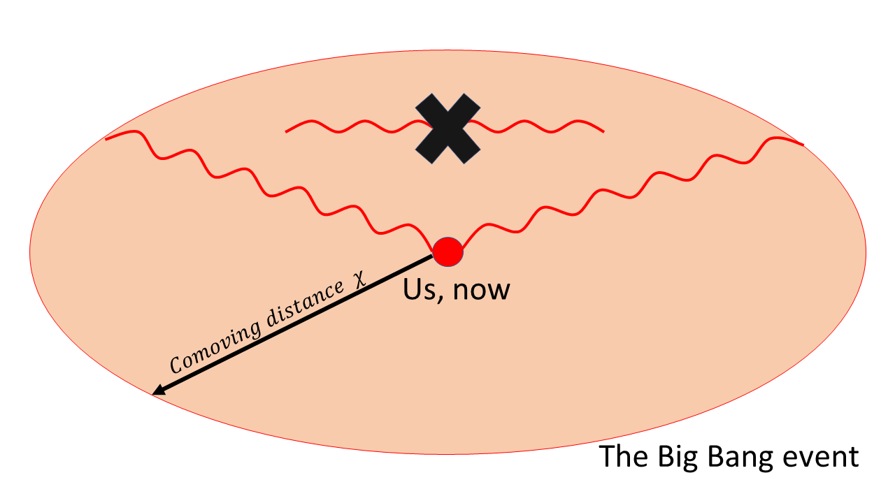
The horizon problem can roughly be put as the following: if we are now at the light horizon of the ancient "Big Bang" event, the information that is propagated to us from one end of the CMB, cannot propagate to the other end of the CMB. Thus these two patches of CMB cannot possibly have exchanged information during the expansion period of the universe (See Fig. 1.1). However, they are thermalized and homogeneous to one part in . If they can’t exchange information how is that possible?
Formalising this requires to consider the Friedmann-Robertson-Walker (FRW) metric:
| (1.1) |
When one considers the distance travelled by light, one sets the interval to zero, thus for light travelling along the axis yielding:
| (1.2) |
So the comoving distance is defined as:
| (1.3) |
where the speed of light is set to , is the scale factor of the FRW metric, which is set such that the current scale is and is the Hubble parameter, which varies for different historical stages of the universe. One of the useful quantities to define is conformal time, in which we rewrite the FRW metric as follows:
| (1.4) |
so is the comoving distance. So, roughly speaking, unless we are in a closed universe which is enclosed within a fully connected sphere of radius no more than the observed , there are patches in the CMB that are causally disconnected. Since these patches are unable to exchange information since the Big Bang event, how can they be in thermal equilibrium with each other? Yet we observe them to be in thermal equilibrium up to one part in .
1.2.2 The flatness problem
Suppose we want to measure distances between different CMB patches. Since we are limited to a two-dimensional spherical view of the CMB, it is intuitive to measure distance by the connection between angle and arc length:
| (1.5) |
where is the arc length, is called the angular diameter distance, and is the angle subtended. In a completely flat universe Eq. (1.3) is connected to by:
| (1.6) |
However, if we live in an open or closed universe in which the curvature is non-zero, the proper generalization is given by:
| (1.9) |
where is the curvature density, and is the current Hubble parameter. While the energy density in radiation scales as , and matter density scales as , the energy density in curvature scales as . This means that if we can construct a scale ladder spanning several epochs, in which sufficiently changes, we can assess the energy density in curvature. Such a ladder is provided to us by Type Ia Supernovae Riess:1994nx; Dunkley:2008ie, and so we are able to evaluate the luminosity distance to an object and compare it to the angular distance . By observing a large sample of these pairs we can extract the overall behaviour of at different times, and which of the three angular distance functions are the best fit. Using this method the most recent Planck data sets the curvature density at
| (1.10) |
This value is very close to zero, which means a flat universe. Of all possible values the curvature density can take, which can be of the order , corresponding to a universe dominated by the curvature component, why is it that we find our universe so close to a flat one? This is not the most finely-tuned quantity in our universe Carroll:2014uoa, but it is fine-tuned nonetheless.
1.2.3 The relic problem
Every Grand-Unified-Theory (GUT) that includes electromagnetism inevitably produces super-heavy magnetic monopoles Zeldovich:1978wj; PhysRevLett.43.1365; PhysRevLett.44.631; mukhanov2005physical, typically of magnetic charge , where is the fundamental electric charge and is of order . Such a large magnetic charge would have observable effects on the universe and would be easily detectable. However so far we have not found any such effect and deduce the lack of any monopoles in the observed universe. During the GUT phase of the universe, the energy density in magnetic monopoles should have been such that today we should have measured . How is it possible that we detect no monopoles then?
1.3 Inflation saves the day
It was Starobinsky Starobinsky:1979ty closely followed by Guth GuthInflation, that suggested the idea of inflation, an epoch of rapid and accelerated expansion of the universe. This mechanism at once fixes the above problems. Let us consider:
| (1.11) |
which is the logarithmic integral of the comoving Hubble radius. When the distance between two objects is larger than the comoving Hubble radius, they cannot currently be in causal connection with each other. If particles are however separated from each other by more than they could have never exchanged information. If we can find a way in which two particles are currently separated more than the comoving Hubble radius, but separated by less than , we can solve the horizon problem. In other words, we want today:
| (1.12) |
and a scale at some time in the evolution of the universe such that
| (1.13) |
Thus there is a phase in cosmic history where the term is increasing:
| (1.14) |
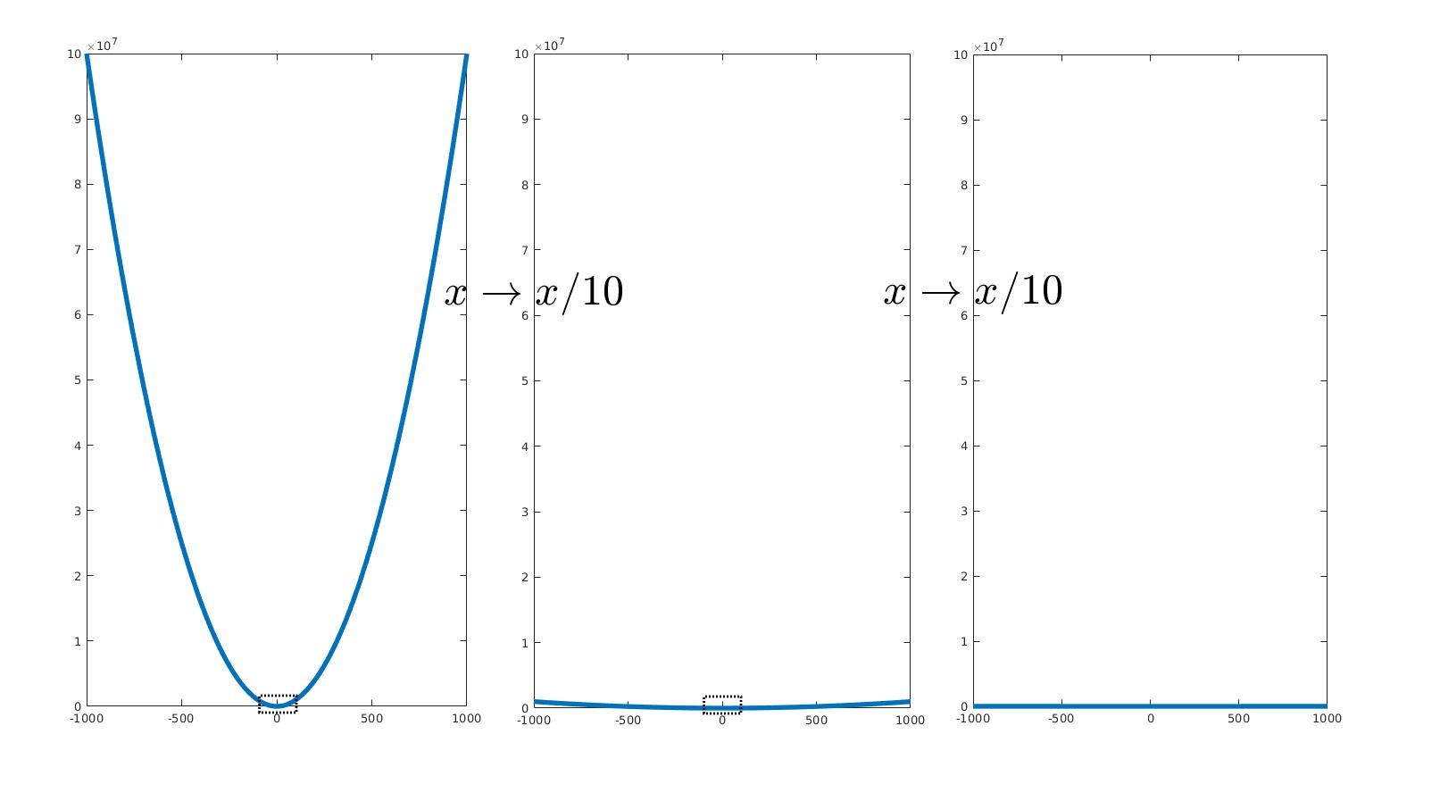
which means the scale factor of the universe was growing in an accelerated fashion. However, this could not have occurred during matter or radiation dominated eras, so there is something else that gives rise to this phenomenon. This solution to the horizon problem naturally solves the flatness problem as well as the relic problem. Rarefying the energy density stored in curvature, by accelerated growth of the scale of the universe, the currently observed curvature strongly tends towards zero. This is similar to the process of deriving a smooth function. By sufficiently ’zooming-in’ (), the curvature vanishes, and we are left with the linear term alone. Similarly, a universe initially populated by relics could have been sufficiently diluted such that we do not observe any relics today.
1.3.1 Features of inflation
There are additional consequences for a period of accelerated growth of the scale factor, beyond the observations suggested above. Perhaps one of the most looked at today is the notion of primordial gravitational waves. In a later section we will quantitatively look at the production of gravitational waves from inflation. However, at this point we want to look at the general idea. Gravitational waves are generated whenever the metric at some point in space undergoes acceleration and is not completely uniform. To see that clearly we consider small perturbations over the flat Minkowski metric:
| (1.15) |
We then define the trace-reversed perturbation:
| (1.16) |
Moving to the transverse-traceless gauge we get:
| (1.17) |
By then using the Lorentz gauge we set:
| (1.18) |
We thus get the following a linearized version of the Einstein equation, which is just a non-homogeneous wave equation:
| (1.19) |
where is the stress-energy tensor. Solving this equation is possible by finding the Green’s function for the wave equation, and incorporating a retarded quantity . Finally, the term for gravitational wave production is proportional to the second temporal derivative of the Quadrupole moment of the energy density:
| (1.20) |
This is not the main focus of this manuscript, however we clearly see that when we have an accelerating quadrupole moment, like in inflation, we have gravitational wave production. The physics that source primordial GW is slight spatial perturbation in curvature, sourced by slight quantum perturbation of the inflaton field. The common notion is that these perturbations are small such that the overall scale factor is given by (no spatial dependence). The way to derive these equations is to consider the FRW metric with slight spatial perturbation such that:
| (1.24) |
Going on calculate the Christoffel symbols, Ricci tensor and scalar and throwing out second amd higher order terms, we get a linearized EFE. The zero-order contribution are the leading order Friedmann equations. Replacing the spatial derivative terms with by going into spatial Fourier-space and after some algebra we arrive at:
| (1.25) |
Rephrased in conformal time, this takes on the follwoing form:
| (1.26) |
where and the prime repesents . It is beneficial to recast this equation into a harmonic oscillator form. To do this we redefine:
| (1.27) |
where the numerical coefficient comes from physical Action considerations. Disregarding this numerical coffeicient we have:
| (1.28) | |||
| (1.29) | |||
| (1.30) |
Inserting these into Eq. (1.26), yields:
| (1.31) |
This equation is similar to the Mukhanov-Sasaki (MS) equation, to be discussed later, that governs the production of scalar perturbation. However the pump field in this equation is the scale factor , whereas the pump field in the MS equation is .
1.4 Solving inflation
Let us first take a look at the simplest form of inflation: A constant energy density term over an FRW background metric. This is also known as the de-Sitter case. In this case the metric is given by where the metric itself is time dependent. Since the system is explicitly time dependent, using a Hamiltonian formalism is disfavoured. Thus we use the Einstein Field Equations:
| (1.32) |
along with the Lagrangian formulation for the equations of motion of the associated fields. When we ’solve’ inflation we intend to say, we calculate the evolution of all inflationary quantities, which in this case are from which we construct all associated quantities: , as well as the slow-roll parameters as defined (, etc.) versus as potential and derivative terms ( etc.) We also construct the pump field that is later used for the quantum perturbations calculation:
| (1.33) |
1.4.1 General Relativity, Friedmann equations in conformal and cosmic time
General Relativity, has shifted our understanding of gravitation from that of a force, to that of a characteristic of space-time, where the force of gravitation is nothing but Newton’s first law as applied in curvilinear coordinates(carroll2003spacetime, Chapter 1).
This is done by coupling a metric (i.e. a manifold that describes space-time) to the total energy present.
This is encoded mathematically by using (psuedo) Riemannian geometry, most commonly using the Einstein notation:
| (1.34) |
where is the Ricci Tensor (2nd order Tensor form), and is the Ricci scalar which is given by:
| (1.35) |
These might sometimes be simplified by using the Einstein tensor:
| (1.36) |
thus we arrive at the form:
| (1.37) |
These applied to the universe as a whole yield the Friedmann equations.
FRW metric and Friedmann equations - cosmic time
The Friedmann-Robertson-Walker metric (FRW metric) is given by allowing the spatial coordinates to change scale, as a function of time. In Cartesian coordinates, this takes on the form of:
| (1.42) |
After going through the process of deriving the Ricci Tensor and Scalar, this metric gives two equations. Taking the temporal-temporal coordinate (), and any of the spatial-spatial coordinate () we have:
| (1.43) | |||
| (1.44) |
where we use the diagonalized Stress-Energy tensor:
| (1.49) |
with
| (1.54) |
This is where one usually points out the possibility of an accelerated expansion/contraction solution to the Friedmann equation. This is given by an energy density term, which is constant, i.e.:
| (1.55) | |||
Ultimately we are dealing with the positive exponential solution since this fits the observations, and solves the Horizon and Flatness problems as previously explained.
However a constant means permanent inflation, so has to change in time, albeit slowly enough to facilitate exponential inflation. This is called the slow-roll condition. It will be discussed at length in section 1.5.
FRW metric and Friedmann equations - conformal time
Moving to conformal time, puts the time coordinate on equal footing with the other spatial coordinates by defining:
| (1.56) |
Thus the interval, or line element, takes on the form of:
| (1.57) |
so, in essence we are reducing the problem to Minkowski space over a time dependant overall scale factor.
In this context, the metric is given by:
| (1.66) |
and the derived Friedmann equations are given by:
| (1.67) | |||
| (1.68) |
It is interesting to see that a constant in conformal time produces the following solution:
| (1.69) |
which explodes to infinity at , thus experiences greater than exponential growth in conformal time. While analytically this stands on equal footing with a cosmic time solution, numerical integration considerations will later lead us to prefer cosmic over conformal time.
1.4.2 The scalar field inflation
Inflation is driven by an energy density term that permeates all of space and is slowly varying, even taking into account the rapid expansion of space.
There might be any number of physical drivers that manifest this behavior, but arguably the simplest form of mechanism which gives rise to inflation is the scalar field one. It has been shown by Albrecht and Steinhardt, that a Higgs-like field, can produce such a scalar effective field Albrecht:1982wi.
The simple Lagrangian (density) form of a scalar field is given by:
| (1.70) |
Where the linear term in the potential can be set to zero because we can always redefine such that the derivatives are unchanged and the quadratic term is changed accordingly. It is a similar procedure acting on the interplay between the second and fourth powers of the Lagrangian, that constitutes the Goldstone gauge Boson procedure NamboGoldstonBoson:1960; Goldston:1962, and ultimately the Higgs Mechanism EnglertBrout:1964; Higgs:1964; theRestOfHiggs:1964.
An almost straightforward generalization, using Legendre transform, and going to covariant form yields (dodelson:2003, Page 152):
| (1.71) |
where is the interaction potential. Considering this field to be mostly homogeneous, and disregarding the small perturbations to this quantity, the spatial derivatives vanish, and we are left with:
| (1.72) |
Identifying this term with Eq. (1.54), we may now denote:
| (1.73) | ||||
| (1.74) |
which is in cosmic time FRW. The conformal time version is given in Eq. (1.81,1.82)
from here on we will forego the superscript (0) for simplicity
1.4.3 Equations of motion
When one is tasked with simulating inflation, whether numerically or analytically, the first step is to evaluate the equations of motion for the scale factor , , and the driving fields, in our case the inflaton . This is done by following these steps:
-
•
Derive Friedmann equations from metric assumptions (FRW/FRW+conformal).
-
•
Replace the quantities and with the driving fields equivalents.
-
•
Identify the set of differential equations to work with.
We now proceed to do so, for a conformal background geometry, driven by a scalar field.
The metric is:
| (1.79) |
and the Stress-Energy tensor for a scalar field is given by:
| (1.80) |
These imply - in conformal time:
| (1.81) | |||
| (1.82) |
With the two equations which we get from the Einstein field equations (EFE):
| (1.83) | |||
| (1.84) |
one can work through the algebra, to get:
| (1.90) |
Since the first two are second order differential equations, and since is not observable, it might be useful to integrate over as defined by . For this aim the second equation is given by:
| (1.91) |
To conclude, in conformal time, a "good" integration scheme might use this set of equations:
| (1.95) |
Deriving the analogue in cosmic time gives:
| (1.101) |
with an equation for given by:
| (1.102) |
where the quantity is neatly wrapped in the term , the reduced Planck mass.
Thus we are left to solve this set of coupled ordinary differential equations (ODE), to resolve the evolution of the background geometry:
| (1.105) |
1.5 The slow-roll paradigm
As was alluded to before when we have a constant energy density term the solution for the temporal-temporal Friedmann equation over an FRW metric is given by:
| (1.106) |
Since is just some constant we can now unpack and solve for :
| (1.108) | |||
| (1.109) |
It is customary to disregard the exponentially suppressed solution since they would be undetected in 2-3 efolds of inflation. Thus we arrive at the pure de-Sitter (dS) solution:
| (1.110) |
This gives rise to the idea of inflation as a phase of an exponent-like evolution of the universe, with an energy density that changes slow enough, to facilitate a perturbative solution, over the baseline of a pure de-Sitter evolution.
1.5.1 Quantifying slow-roll
One way to quantify slow-roll would be to assume the basic solution for is an exponent function, and then use perturbations over that baseline such that , , and go on in a perturbative expansion. However, the usual formalism that is used to quantify slow-roll is based on the idea that the Hubble parameter should be very slowly changing with respect to cosmic time. This means that the perturbative degrees are applied to rather than . It ,therefore, makes sense to write as some power series in .
Taylor expansion
As it turns out since has units of , i.e. is the reciprocal of cosmic time, it makes sense to develop the function in a Taylor series around , where is a constant. Thus we have:
| (1.111) |
The first slow-roll parameter can be read directly from the above expansion:
| (1.112) |
and it is usually, within the framework of slow-roll inflation, small and positive since it is understood that, naturally, the average energy density should decline as the universe inflates. This leads to slightly decrease, thus slightly increasing . We are left, then, with a positive first-order contribution to the Hubble horizon. Formally slow-roll takes place when
| (1.113) |
The second term in the Taylor expansion needs a bit of handling to find a more aesthetic term.
The slow-roll parameters and
While the first slow-roll parameter is a small, non-negative quantity, given simply by (1.112), in order to simplify the second slow-roll parameter we need to refer to the Klein-Gordon equation for a time-dependent scalar field (1.101, top equation). Reason states that where the field is slowly rolling, the drag term that is given by , roughly counteracts the force term , leading to a terminal velocity-like state. In that scenario the fields ’acceleration’ is roughly zero, so we get:
| (1.114) |
differently stated as
| (1.115) |
It makes sense, then, to look at the dimensionless quantity
| (1.116) |
and set an additional slow-roll condition as
| (1.117) |
The connection with the Taylor expansion is not immediately obvious, so we will explicitly derive it. The second order term in the Taylor expansion for is given by:
| (1.118) |
Let us examine this term:
| (1.119) | |||
Thus the aforementioned term (1.118) is given by:
| (1.120) |
and the Taylor expansion up to second order is given by:
| (1.121) |
where the expansion is around .
Switching gears into and
It is beneficial for theoretical physicists to be able to connect the slow-roll parameters directly to the inflationary potential. This is done because as we shall see the primordial power spectrum can be quantified up to several percent precision, directly by the slow-roll parameters. The first slow-roll parameter in potential and potential derivative language is usually given by
| (1.122) |
The two definitions, and coincide in both extreme limits, i.e. when slow-roll is extremely slow and strictly vanishes and , and at the other end of inflation, where is no longer slowly varying, and the accelerated evolution of the scale factor vanishes (). The derivation of the slow-roll parameter is as follows: In slow-roll inflation, the potential overpowers the kinetic energy immensely thus:
This simplifies greatly the two major players of inflation, the first of which is:
The second equation, the equation of motion for the scalar field is usually given by:
which is the result of derivation with respect to time of the more primitive form of:
So now, seeing as the first term on the left is dominated by we can set:
And deriving with respect do time we have:
Now we remind ourselves that and that to get:
or in its elegant form:
So, to sum it up we have:
From the second we get , and since we have:
and so we have:
as long as we are in slow-roll. We want to pay attention though to the assumption in which , when this assumption is weaker, we need additional terms to mitigate between and . In fact, later we will make the adjustments up to second order and supply a ’recipe’ to extend this to higher orders as well. By the same kind of process we can look at the term:
| (1.123) |
Since we know that we can now derive with respect to and get:
| (1.124) |
Thus the quantity
| (1.125) |
which is to say, if we define as
| (1.126) |
we have
| (1.127) |
1.5.2 First-order scalar perturbation theory
In the previous sections, we have used the Einstein Field Equations, as well as a Stress-Energy tensor for a scalar field. The procedure for deriving the Mukhanov-Sasaki equation uses a first-order perturbation approach to the EFE’s.
We shall go through the main parts, but only in general, whereas the detailed process is demoted to an appendix status. It should be noted that, in general, we follow Mukhanov’s derivation as outlined in Mukhanov1992203.
We use the conformal metric - , where is the Minkowski metric, and is a small perturbation of the form:
| (1.131) |
The Action for the scalar field is given by:
| (1.133) |
Varying the Action with respect to yields the equations of motion for which are nothing but the Klein-Gordon equation for in conformal time:
| (1.134) |
Where, using a perturbed conformal metric, as well as a first-order perturbed gives additional information:
| (1.136) |
The equations , can be broken into perturbative degrees:
| (1.141) |
where the leading-order perturbations in the Stress-Energy tensor are:
| (1.145) |
and the corresponding perturbed Einstein tensor, after proving in our case, is given by:
| (1.151) |
Using these to compile 3 equations, and using the equations of motion for we are left with:
| (1.152) |
Or in an equivalent form:
| (1.153) |
Switching to a new variable , with this equation now takes the form:
| (1.154) |
This is the Mukhanov-Sasaki equation.
To simplify the solution of this equation we decompose unto Fourier modes , going into Fourier space we get:
| (1.155) |
and when we go to Fourier space the pump field in the original space, , becomes the pump field in Fourier space
| (1.156) |
We can wrap up the quantity as follows:
| (1.157) |
so the MS equation can be expressed as:
| (1.158) |
In this form it is easily recognized as a Time-Dependent Harmonic Oscillator (TDHO).
1.6 The primordial power spectrum - a signature of our history
The patterns we currently see in the CMB, are remnants of the time of last scattering. The CMB photons that are just now detected in our instruments were last scattered when the universe was approximately times smaller and hotter. At that time the different constituents of the universe were in thermal equilibrium. Photons were scattered off electrons, and in turn, electrons were constantly bombarded with photons. In such a state matter is in a plasma phase, the optical depth is very small and whatever information a photon carries is erased after a few interactions. The current working assumption is that the optical depth increased suddenly, due to a sudden temperature drop that enabled electrons to be captured into previously ionized hydrogen atoms. At that point, the photons were no longer tightly coupled to electrons and were free to escape. It is these photons that first broke free that we now collect in our CMB instruments.
1.6.1 Matter power spectrum
However, since the time of last scattering several mechanisms have affected photons over time. It is customary to decompose the CMB radiation to modes, each corresponding to a different physical scale. The smallest -mode we can hope to detect now corresponds to the scale of the current universe. The mode that is just now becoming causally connected corresponds to the current light horizon size. It can be shown that any region separated by more than 2 degrees in the sky today would have been causally disconnected at the time of decoupling Liddle:1999mq. Modes that are not yet causally connected are ’frozen’ and are roughly measured "as-is". Conversely, causally connected modes can now discharge energy, dissipate, or otherwise interact with other energy constituents of the universe. As such the CMB we currently detect differs from the radiation at the time of last scattering.
1.6.2 Transfer function
In order to reflect the different physical processes sub-horizon and super-horizon modes undergo, as well as the overall expansion of the universe, which affect all modes, the Transfer function is called for. Given an initial power spectrum at the time of last scattering:
| (1.159) |
where here is the matter power spectrum, is the PPS, is the transfer function, and is the growth function, which is dependent only on , and reflects the change in modes due to the overall increase in the scale factor of the universe.
1.6.3 Scalar power spectrum
The primordial power spectrum (PPS) is traditionally characterized by its spectral index and the index running , which are given by the first and second logarithmic derivatives of the logarithm of the PPS:
| (1.160) |
| (1.161) |
where denotes the CMB scale. Extending this Taylor expansion, we can write the PPS as:
| (1.162) |
where is the scale around which we Taylor expand, and is called the pivot scale. is the next term in the Taylor expansion and is called the running of running. It is given by:
| (1.163) |
In most places the subscript denoting the assessment of the power spectrum at is suppressed.
1.7 Stewart-Lyth power spectrum
1.7.1 Derivation
Here we retrace the procedure of deriving the most widely used analytical expression for . Recalling the definition for the pump field , and the MS equation (Eqs. (1.156),(1.155)). The parameter is properly defined as:
| (1.164) |
However, in the Stewart-Lyth (SL) formulation, the approximations made lead to the definition of as the somewhat different:
| (1.165) |
Then the MS equation becomes:
| (1.166) |
For a constant this becomes the Bessel equation, with known solutions. The value of is formally given by:
| (1.167) |
In many cases, one assumes that the time derivatives are small and can be neglected. However, these derivatives yield second-order terms that can significantly affect the value of . The full expression is given by:
| (1.168) |
which may differ from Eq. (1.167) after removing the time derivative terms, when and/or are non-negligible. is usually of the order of or less, even for models with high .
Applying boundary conditions and taking the small arguments limit we are left with a power spectrum of:
| (1.169) | ||||
which yields the scalar index of:
| (1.170) |
with the digamma function . The final expression is heavily dependent on the value and time derivative of . This is a possible source of inaccuracy. In the original text the author now define:
| (1.172) |
Having defined these, usually one connects the original slow-roll parameters with the above quantities by Stewart:1993bc
| (1.178) |
With these relations, one can substitute the slow-roll parameters in Eq. (1.170), for the quantities in Eq. (1.178), to get the most commonly used analytical expression for the scalar index Lyth:1998xn:
| (1.179) |
where , and , being the Euler number.
1.7.2 Analytical term for index running
Following the same procedure for the running of the scalar index, gives, to second-order:
| (1.180) |
where both (1.179), and (1.180), are evaluated at the CMB point if one wishes to probe the CMB point. Equivalently if one wishes to compare to observables as derived from MCMC analyses at some pivot scale , one needs to find the correct , and evaluate these expressions at the pivot scale.
1.8 Other formulations for the power spectrum observables
In this section, attention should be paid to different formulations and notations. Every subsection is self-contained to encapsulate the derivations fully. Wherever possible we use the notation in the source material. Over the years, our observations have become more accurate and spanned a longer interval of physical scales Bennett:2003ba; Leitch:2001yx; Halverson:2001yy; Pryke:2001yz; Netterfield:2001yq; deBernardis:2001mjh; Lee:2001yp; Stompor:2001xf; Tegmark:2000qy; Hannestad:2001nu. Even well before the Planck mission Planck:2006aa was proposed and eventually launched, the prospects of probing not just the slope of the PPS but the running of the slope was compelling. As a result, several forays into calculating the running of the spectral index were made. It was understood early on, that Eq. (1.180), was put forth as a second order derivation of an expression that by definition vanishes. As a result different approaches were taken, at the level of analytic expression for the PPS itself, rather than calculating derivatives of the it predicts. All of these attempts were made around 2011.
1.8.1 Dodelson-Stewart
Twin papers written by Ewan Stewart and Scott Dodelson were published in September and October of 2011. Stewart published a detailed calculation of the PPS Stewart:2001cd, dropping a previous assumption, that . Dodelson and Stewart published a joint paper, based on the calculations made in Stewart:2001cd, that studies the ramifications of these formulae on inflationary potentials Dodelson:2001sh. This treatment uses the slow-roll parameters in the efold-flow formulation, such that:
| (1.181) |
and their evolution is governed by:
| (1.182) | |||
| (1.183) |
In this approximation the scalar index is given by:
| (1.184) |
where are numerical coefficients of order unity, and the remainder includes the terms and . These terms can be calculated by using the following generating function:
| (1.185) |
In this formulation the scalar index running is given by:
| (1.186) |
In terms of inflationary potential and derivatives thereof, the scalar index and the index running are given by:
| (1.187) | |||
| (1.188) |
where here are generated by the following generating function:
| (1.189) |
As we shall see this formulation is close, but only in the ’horseshoes and hand grenades’ sense.
1.8.2 Stewart-Gong
The Stewart-Gong formulation Gong:2001he is, in essence, similar. They first set up the Green’s function formalism to tackle the problem of inflation. They rewrite the MS equation Eq. (1.155) as:
| (1.190) |
where and are defined as111Note that in this derivation denotes conformal time:
| (1.191) | |||
| (1.192) |
They then choose the ansatz , where is some function. Defining a new function such that:
| (1.193) |
the equation of motion now transforms to:
| (1.194) |
Now we can take the Green’s function approach to get the eigenfunction , and yield the full solution:
| (1.195) |
The authors continue to write the full expression for :
| (1.196) | ||||
where the hierarchy of slow-roll parameters is defined as:
| (1.197) |
At the end of this formulation, as we shall see, lay no cigars as well.
It is, however, worth mentioning, that Dvorkin & Hu Dvorkin:2009ne, used this method iteratively to calculate the PPS to accuracy.
1.8.3 Schwarz-Escalante-Garcia
The formulation in Schwarz:2001vv claims not to rely on the slow-roll expansion, but as we shall see this is not accurate. We first define the horizon flow parameters as:
| (1.198) |
where is the Hubble distance, and is the Hubble distance at the start of inflation (at , where ). The hierarchy of functions is defined as:
| (1.199) |
According to this definition, , and it can be shown that
| (1.200) |
Upon closer inspection, one finds this is nothing but a rewriting of the slow-roll parameters of Eq. (1.197), as shown in table .1.1.
| Schwarz-Escalante-Garcia | Stewart-Gong |
|---|---|
As such their analysis is not so different from previous ones made. However, they provide a taxonomy of models which divide models into two categories: Constant-Horizon (CH) models, and Growing-Horizon (GH) models. The CH category is reserved for models that have a very small time derivative of the Hubble distance. This implies that , but it doesn’t necessarily mean that is small for arbitrary . Thus the authors define as models in which . In this case, the following terms are allowed in the approximation: . In the GH treatment, the approximation scheme is different. This scheme is inspired by the power-law inflation case in which , for inflation with , and the other slow-roll parameters strictly vanish. Thus this scheme defines as the maximal integer in which holds true. So the slow-roll terms allowed in this approximation scheme are .
The power spectra given in the CH case are given by:
| (1.201) | ||||||
| (1.202) | ||||||
| (1.203) | ||||||
| (1.204) | ||||||
| (1.205) | ||||||
with the same as before: , and where . The power spectra of GH models are given by:
| (1.206) | ||||||
| (1.207) | ||||||
| (1.208) | ||||||
| (1.209) | ||||||
| (1.210) | ||||||
with the same values of and .
While this approach at least gives us consistent conditions for the voracity of different approximation schemes, it is no closer to the mark than the previous ones.
1.9 The Lyth bound, original and extended versions
One of the most useful heuristics out there, to build and evaluate inflationary models, is the so-called Lyth bound. In the original paper Lyth:1996im, there are several conclusions. However we concentrate on the following argument: Given that the PPS can be written as
| (1.211) |
and the tensor power spectrum is given by:
| (1.212) |
we can define the tensor-to-scalar ratio, , as the power spectra ratio at some scale of our choosing. Thus is set as:
| (1.213) |
The numerical coefficient is subject to some finer detail, but the order of magnitute is always the same. In Lyth:1996im we have , whereas other sources state . This statement, along with the (extreme) slow-roll assumption in which yields the following:
| (1.214) |
In order to complete the argument, we must look at the quantity
| (1.215) |
So, plugging in the former equation we get:
| (1.216) |
where we adhere to the numerical coefficient in Lyth:1996im.
The scales on which the tensor power spectrum is most prominent, and therefore is more likely to be discovered at is . With , the interval in -space over which we expect to find tensor modes is . Taking to be roughly constant, when we evaluate we have
| (1.217) |
thus
If we additionally take to be approximately constant along the aforementioned -interval we have:
| (1.218) |
Putting these together yields:
| (1.219) |
This means that given some we can approximate the field excursion, in Planck units, during the first efolds of inflation. For example, suppose we find , which is possible in the foreseeable future. In that scenario we have:
| (1.220) |
Applying Eq. (1.214), we can also get a one-to-one relation between and the slope of the potential at a chosen , as long as is inside the window. This relation is formalized in BenDayan:2009kv as
| (1.221) |
where the numerical coefficient is subject to slight changes, and the minus sign comes from the notion of the field rolling towards the larger positive values.
This original argument was extended in Easther:2006qu; Efstathiou:2005tq. In Easther:2006qu, the argument was amended to include higher slow-roll parameters, to allow for models that change by a significant amount during the tensor mode window. This extended Lyth bound is given by:
| (1.222) |
and in the case of we have . In Efstathiou:2005tq however, some assumptions were added, in order to extend the bound to the full efold extent of inflation, i.e. . In this case the authors extend the Lyth bound such that:
| (1.223) |
This would imply that models that predict , should incur a field excursion of .
1.10 Small and Large field models taxonomy
Current nomenclature distinguishes between ’Large field models’ and ’Small field models’. This distinction is based on Dodelson:1997hr, where several models were studied and a taxonomy of models was presented. In the interest of brevity and accessibility, we will first reiterate the key concepts needed to understand this distinction. First, the slow-roll condition on the potential is given by:
| (1.224) |
where , and usually it is understood as a strong requirement i.e. we prefer , in order to be in the slow-roll regime. The number of efolds generated within a certain inflation is given by:
| (1.225) |
where the minus sign is due to our interpretation of the field rolling down the potential. Finding given the potential is usually straightforward, by setting we identify the end of slow-roll inflation, thus:
| (1.226) |
from which we can extract .
In Dodelson:1997hr, the authors divide the models studied into 3 categories:
-
1.
Large field models: in which the inflaton field is displaced far from its minimum, and rolls down the potential towards a minimum at the origin. The models and are classic examples of large field models.
-
2.
Small field models: in which the field is initially near the origin, and rolls down towards a minima that is removed from the origin (), these types of models would be expected as a result of spontaneous symmetry breaking.
-
3.
Hybrid models of inflation: in which the field evolves towards a minima with a non-zero vacuum energy. Usually, hybrid models are realized with a number of dynamic fields. However during inflation, in most cases one can identify a dominant field, and thus treat this type of models as single field inflation models, at least a posteriori. We do not discuss hybrid models of inflation within the context of this work.
1.10.1 Large field models
Since these type of models, as defined in Dodelson:1997hr, usually have initial values of or more, the taxonomy had evolved to the following simplified meaning. Large field models are models in which the field excursion during inflation is more than a few . Let us examine the class of Large field polynomial potentials to understand why that is:
| (1.227) |
By virtue of Eq. (1.226) we have , and by applying Eq. (1.225), we recover the following condition on the initial value:
| (1.228) |
With , and even when , this produces and approximately the same. Thus in these models . With the exponential models the end of inflation occurs near . The relation between the starting and end positions of the field is given by:
| (1.229) |
and a quick inspection of this as a function of reveals a minimum at , which means the minimum field excursion is given by:
| (1.230) |
when . This is enough to justify the notion of large field models, as models in which the field excursion during inflation is of several Planck masses.
1.10.2 Small field models
The methodology of evaluating small field models is the same as the above, with the only difference of starting near the origin:
| (1.231) |
The usual representative of this class of models is the "small-field polynomial model"
| (1.232) |
This model is not to be confused with the models we study, as it is actually a monomial, meaning there is only one term in which appears. Note that since this is the most usual representative of the small field models, there is a tendency to study this class and apply these conclusions to the entire class. This is evident in Martin:2013tda for example. In these types of models it is easily discerned that the field excursion can be of the order of , and usually much smaller.
A different more observable-oriented classification of models can be found in Schwarz:2004tz.
Chapter 2 Our Models
Small field models of inflation in which inflation occurs near a flat feature, a maxima, or a saddle point are studied (see Boubekeur:2005zm for a review). This class of models is interesting because they appear in many fundamental physics frameworks, effective field theory, supergravity Yamaguchi:2011kg and string theory Baumann:2014nda in successive order of complexity. Our focus on such models is also motivated by the expected properties of the moduli potentials in string theory. More generally speaking these type of models can be viewed as a Taylor expansion approach to other models Dodelson:1997hr. A different more observable-oriented classification of models can be found in Schwarz:2004tz, in which analysis our models fall into the toward-exit class.
In general, inflation will occur in a multi-dimensional space. However, the results for multifield inflation cannot usually be obtained simply. In many known cases, it is possible to identify a-posteriori a single degree of freedom along which inflation takes place. To gain some insight about the expected typical results effective single field potentials can be used.
Generic small field models predict a red spectrum of scalar perturbations, negligible spectral index running and non-gaussianity. They also predict a characteristic suppression of tensor perturbations BenDayan:2008dv. Hence, they were not viewed as candidate models for high- inflation. Large field models of inflation are thus the standard candidates for high- inflation. For more detailed model building considerations one can review Makarov:2005uh and Lesgourgues:1998mq.
In BenDayan:2009kv, a new class of more complicated single small field models of inflation was considered (see also Hotchkiss:2011gz) that can predict, contrary to popular wisdom Lyth:1996im; Martin:2013tda, an observable GW signal in the CMB (see also Cicoli:2008gp.) The notion that observable signal GW precludes small field models partly stems from Martin:2013tda and similar analyses that study monomial potential models as small field models. The spectral index, it’s running, the tensor to scalar ratio and the number of e-folds were claimed to cover all the parameter space currently allowed by cosmological observations. The main feature of these models is that the high value of is accompanied by a relatively strong scale dependence of the resulting power spectrum. Another unique feature of models in this class is their ability to predict, again contrary to popular wisdom Easther:2006tv, a negative spectral index running. The single observable consequence that seems common to all single field models is the negligible amount of non-gaussianity.
In Lesgourgues:2007gp the inflationary potential was Taylor-expanded up to order . The approach applied in Lesgourgues:2007gp is similar to ours, however only potentials that are monotonic in the entire CMB window were considered. The family of potentials we study can easily contain members that have a shallow minimum point followed by an equally shallow maximum. As long as there is enough kinetic energy to clear that interval in , we will clear the potential ‘valley’ and not be trapped in a scenario where inflation doesn’t end. A concrete example would be a third degree small field monomial of the form , after a shift such that . In this case and terms will appear in the shifted potential. Following this shift it is an easy matter to add some small terms of degree four, five and six to the potential, such that we get a six degree polynomial member with a shallow minimum. Though we haven’t targeted potentials with minima especially, we have not ruled these out a-priori, thus some potentials as the one in the example were manufactured by the computerized model building package, and were tested for compliance.
The current work yields corrected predictions of this class of models by a systematic high-precision analysis, thus providing a viable alternative to the large field-high option. The analysis of BenDayan:2009kv is extended, in preparation for a subsequent detailed comparison of the models to data. This is done in order to simplify the parametrization of the potential and facilitate a comprehensive numerical study.
2.0.1 Inflaton potentials with
The following class of polynomial inflationary potentials proposed in BenDayan:2009kv is:
| (2.1) |
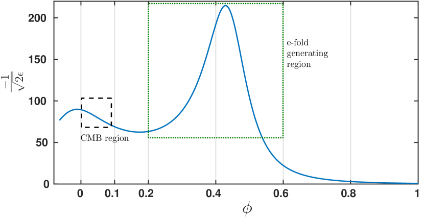
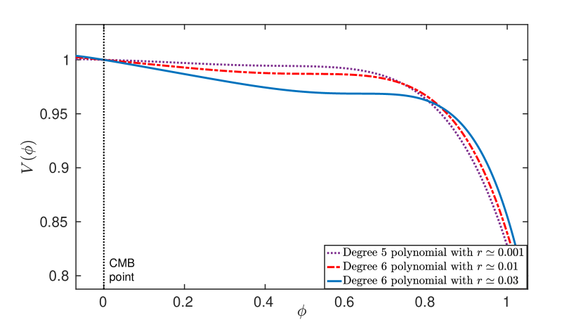
The virtue of these models from a phenomenological point-of-view is the ability to separate the CMB region from the region of large e-fold production. Hence, these potentials can produce a very different spectrum early on, than in the later stages of inflation. Fig. 2.1 illustrates this point, with separate CMB region and e-fold generation region. In the context of both classification systems mentioned, current observational data weakly support these Martin:2014lra; Vennin:2015eaa. However the small field model studied in Martin:2014lra are monomial potential models of the form , which are different from many of our models.
In many models, , , and the time derivative can approximately be replaced with a factor of Kosowsky:1995aa. In the above models, this standard hierarchal dependence is broken, they have a more complicated dependence while obeying the slow-roll conditions , . In BenDayan:2009kv it was shown that these models can be written as:
| (2.2) |
Here , are defined as , , , respectively. The subscript means that these are the values at the CMB point.
2.0.2 Reduced parameter space
The potential in Eq. (2.2) is a small field candidate, which after some scaling and normalization, depends on four free parameters. One parameter is used for setting at the CMB point, and thus the predicted amplitude of the GW signal produced, while the other two parameters are used to parametrize the -plane. The fourth parameter determines the number of e-folds from the CMB point to the end of inflation. is set to to simplify the analysis. It follows that
| (2.5) |
Suppose we want inflation to end at , we can rescale :
| (2.6) |
In this formulation,
| (2.7) |
where . Since this is the same potential, it follows the same CMB observables are produced. Thus, applying condition (2.5) can be viewed as a scaling scheme for the different terms in the potential which does not limit the generality of our results.
Substituting the expression for the potential and its derivative at we get:
| (2.8) |
is now given in terms of the other coefficients:
| (2.9) |
Using the standard definition for the number of e-folds , and the approximation yields a rough estimate for as a function of ,
| (2.10) |
This estimate is then used as a starting point to refine by solving the background equations iteratively thereby obtaining the accurate coefficient that yields the correct . Thus a 4-dimensional parameter space , , , is defined. The parameters are constrained by the requirement , is constrained by the observable value of and is determined by the other parameters and by the number of e-folds (taken to be in between ). The PPS considered is in the range of the first e-folds of inflation.
2.0.3 Inflaton potentials with
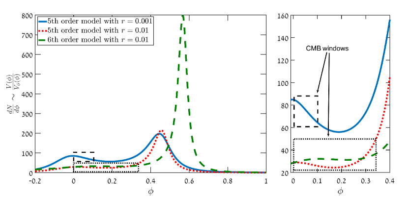
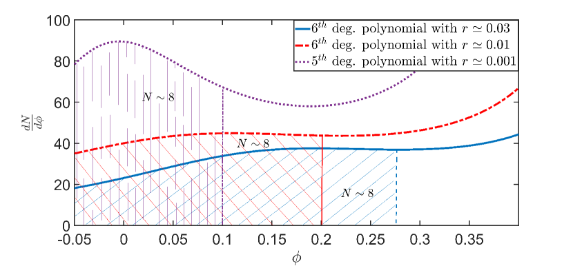
In Wolfson:2016vyx, a class of small field inflationary models which can reproduce the currently measured CMB observables, while also generating an appreciable primordial GW signal was studied. The existence of such small field models provides a viable alternative to the large field models that generate a high Tensor-to-Scalar ratio. Our exact analysis was shown to give accurate results Wolfson:2016vyx. Models which yield Tensor to Scalar ratio, of less than were previously studied in Wolfson:2016vyx. The initial study additionally demonstrated a significant difference between analytical Stewart-Lyth Stewart:1993bc; Lyth:1998xn estimates and the exact results. This result should be confronted with analyses such as in Martin:2013tda where the Stewart-Lyth expression is relied upon, and Dodelson:2001sh in which the authors use a Green’s function approach and perturbation theory, but assume the log of the input is well behaved. Our method extends and improves the method of the model building technique employed in BenDayan:2009kv; Hotchkiss:2011gz. Previous analytical work Choudhury:2014kma; Chatterjee:2014hna; Choudhury:2015pqa has shown that a fourth-order polynomial potential is sufficient to generate a high tensor-to-scalar ratio, even up to . However, it was hard to realize this numerically. It was discovered in Wolfson:2016vyx, that a fifth-order polynomial potential was required for generating . Furthermore a sixth-order polynomial seems to be required for a tensor-to-scalar ratio greater than . A simple explanation is offered by observing (see Fig. 2.2) that increasing by factor , causes the e-folds per field excursion generated at the CMB window to decrease by a factor of . This means widening the CMB window and losing the decoupling between the CMB window and the e-fold generating peak. Adding the 6th coefficient pushes the peak from , to higher values of and decouples these regions.
2.0.4 Inflaton potentials with
We continue our investigations Wolfson:2016vyx; Wolfson:2018lel of a class of inflationary models that were proposed by Ben-Dayan and Brustein BenDayan:2009kv and were followed by Hotchkiss:2011gz; Antusch:2014cpa; Garcia-Bellido:2014wfa. This class of models is compatible with several fundamental physics considerations. Recently, interest in this class of models was revived by the discussion about the “swampland conjecture", Lehners:2018vgi; Garg:2018reu; Kehagias:2018uem; Ben-Dayan:2018mhe which suggests that small field models are favoured by various string-theoretical considerations (see Palti:2019pca for a recent review).
In addition, for this class of inflationary models, high values of result in a scale dependence of the scalar power spectrum. Future experiments such as Euclid Amendola:2012ys, and SPHEREx Dore:2014cca aim to probe the running of the scalar spectral index at the level of . This is a major improvement in comparison to the Planck bounds on which are currently at the level of . Such future measurements could provide additional constraints on our models.
The small field models that we study are single-field models. The action of such models is given by
| (2.11) |
The metric is of the FRW form and the potential given by
| (2.12) |
Previously, in BenDayan:2009kv; Wolfson:2016vyx this class of models was discussed from a phenomenological and theoretical points of view. In Wolfson:2016vyx, the technical details of model building and simulation methods were discussed, while in Wolfson:2018lel, the analysis and the extraction of the most probable model were discussed. Additionally, in Wolfson:2018lel, the most likely model which yields was identified.
The small field models previously studied in Wolfson:2016vyx yielded results that are consistent with observable data up to values of . While these values agree with the current limits on set by Planck Ade:2015tva; Ade:2015xua, we are interested in studying models with higher . For models with , significant running of running is found. This means that while three free parameters (corresponding to ) were previously needed, we now need an additional free parameter. Therefore we turn to a model of a degree six polynomial potential. Obviously considering higher degree models complicates the analysis by adding other tunable parameters. The potential is given by the following polynomial:
| (2.13) |
It has been shown BenDayan:2009kv that the potential can be written as:
| (2.14) |
However, for simplicity, we express the potential as follows:
| (2.15) |
with the subscript denoting the value at the CMB point. By setting we limit ourselves to small field models in which in Planck units, with little effect on CMB observables. According to the Lyth bound Lyth:1996im; Easther:2006qu, given a Tensor-to-Scalar ratio of , the lower bound on the field excursion is approximately given by . Here is the field excursion while the first efolds are generated. Our models satisfy this strict bound, as the first 4 efolds or so typically result in which is well above . The Lyth bound was further extrapolated Efstathiou:2005tq to cover the entire inflationary period. Applying this approach to models with yields . However, in Hotchkiss:2011gz, it was shown that in models such as the ones we study, the value of can be smaller because is non-monotonic. In this case, from the CMB point to the end of inflation is consistent with the Lyth bound.
When the coefficients are fixed, the remaining coefficients are related by:
| (2.16) | |||
| (2.17) |
The procedure of finding and was explained in detail for the degree 5 polynomial models in Wolfson:2016vyx, and here we follow a similar procedure for the degree 6 models. So, ultimately, the model is parametrized by 5 parameters: the two physical parameters and and the three other parameters () that are used to parametrize the parameter space. It should be pointed out that is not an observable, rather is a ’soft’ constraint. Strictly speaking, depends on the reheating temperature and only its maximum value can be determined. However, for simplicity, we treat as an observable, in order to facilitate the study of a large sample of models.
Chapter 3 Methods
3.0.1 Coefficient extraction methods
In this section, we explain the two methods for calculating the most likely coefficients , given a large number of simulated models and the likelihood data for the CMB observables. This data is available through CosmoMC Lewis:2002ah analysis of CMB data, such as the Planck data Ade:2015tva.
Likelihood assignment method - Gaussian extraction
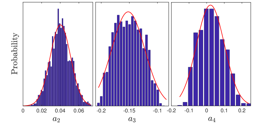
To each potential, after calculating the observables , we assign a likelihood. For each observable, we calculate the likelihood according to the MCMC likelihood analysis of the data sets used. We then assign the product of the likelihoods to the potential. A concrete example is the following: suppose we extract the trio , we look up the likelihoods: . We now multiply them, and so the likelihood attached to that specific model which yielded these observables is given by We proceed to extract likelihoods for the different coefficients by process of marginalization. The expectation is that this method will yield a (roughly) Gaussian distribution for each of the values of . The advantage of this method is in yielding not only the most likely value but also the width of the Gaussian. This width can then be used as an indication for the level of tuning that is needed in these models.
Possible pitfalls
This method of likelihood assignment is vulnerable in two ways:
-
a)
To be valid, this method requires a uniform cover of the relevant parameter space, by the potential parameters. If the cover significantly deviates from uniform, the results might be skewed by overweighting areas of negligible likelihood, or underweighting areas of significant likelihood. Fig. 3.1 shows a mostly uniform cover.
-
b)
Since only if the paired covariance is small, we must make sure that this is the case. In our underlying MCMC analysis this is indeed the case. The covariance terms are, in general, one to two orders of magnitude smaller than the likelihoods at the tails of the Gaussian.
-
c)
We also run the risk of false results if the fit we apply to the data points produced by the numerical analysis yields a large fitting error. However, the fitting error of the polynomial function to the data is usually of the order of . This fitting is done over 30 data points generated by the MS equation numerical evaluation, for each potential. The error is calculated as , thus the error per data point is of the order of . We conclude that the function is well fitted.
Multinomial fit
Another method for calculating the most likely coefficients is by fitting the simulated data with a multinomial function of the CMB observables. We aim to find a set of functions such that, for example, . We assume that this function is smooth and thus can be expanded in the vicinity of the most likely CMB observables. Hence, we can find a set of multinomials , such that:
| (3.4) |
We have found that a quadratic multinomial is sufficiently accurate and that using a higher degree multinomial does not improve the accuracy significantly. Thus we may represent these by a symmetric bilinear form plus a linear term, as follows:
| (3.5) |
where , is the bilinear matrix, and the linear coefficient vector is .
Pivot scale
So far, we discussed matching potentials and their resulting PPS around the CMB point. However, in order to correctly compare the results of the PPS to observables, one has to take into account the pivot scale at which the CMB observables are defined. Since, in this case, the pivot scale is given by , and the CMB point is at , the observables in the CMB point and should be related in a simple way only if the spectrum varies slowly with . This is not true for the case at hand. Two potentials can yield very different power spectra near the CMB point, and nevertheless yield the same observables at the pivot scale. These degeneracies, stem from our limited knowledge of the power spectra on small scales, and at the CMB point. For concreteness take two PPS functions, one that is well approximated by a cubic fit near the pivot scale, and the other that is well approximated only when we consider a quartic fit. Suppose, additionally, that these two PPS functions have the exact same first three coefficients, it follows that they yield the exact same observables . However, if we go to sufficiently small scales or high enough values, these functions will diverge. This is also true at the large scale end, where the CMB point is set. Hence the degeneracy.
A possible solution to this problem is classifying the resulting power spectra by the level of minimal good fit. We define a good fit as one in which the cumulative relative error , is less than . Given a single power spectrum, we fit our result with a polynomial fit, increasing in order until the accumulated relative error is sufficiently small. The minimal degree polynomial fit that approximates the function to the aforementioned accuracy is called the minimal good fit. We then study separately power spectra that are well fitted by cubic polynomials, quartic polynomials etc. In this way we make sure that we compare non-degenerate cases.
3.0.2 Monte Carlo analysis of Cosmic Microwave Background with running of running
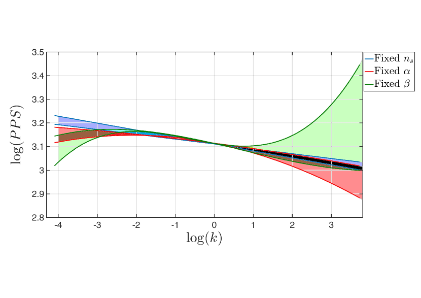
In Cabass:2016ldu it was shown that the inclusion of additional parameters, i.e., the running of the spectral index (), and the running of the running () resolves much of the tension between different data sets. In this section, we briefly discuss the effect of considering non-vanishing and on the most likely shape of the PPS. First, we find when it is the only free parameter. We then use , and as the free parameters, and finally we conduct an analysis with and as the free parameters. The shape of the power spectrum changes significantly when running of running is considered.
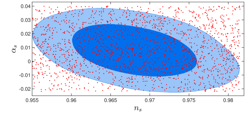
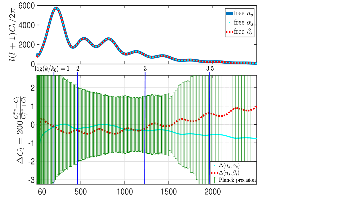
The data sets that were used are the latest BICEP2+Planck baseline Ade:2015tva, along with the low ’s Bennett:2012zja, low TEB and lensing likelihoods. The results of these analyses are given in Table 3.1, as well as in Fig. 3.3. As expected the resulting power spectra converge at the pivot scale . However, for lower ’s, the resulting spectra diverge considerably, consistent with cosmic variance. Notably, the spectra also diverge at higher ’s. This indicates the inability of current observational data to constrain the models in this range of ’s. This inability is also demonstrated in Fig. 3.4 where, for , the most restrictive data cannot rule out models with significant running, or running of running. Figure 3.4 also shows that the three models are virtually indistinguishable in terms of the observed ’s.
The conclusion is that we will need additional accurate data from smaller cosmic scales to be able to differentiate between the three scenarios. These extra e-folds might come from future missions such as Euclid Amendola:2016saw, or -type distortion data Diacoumis:2017hhq; Abitbol:2017vwa.
| Parameter (68%) | free | free | free |
|---|---|---|---|
| N/A | |||
| N/A | N/A |
Chapter 4 The INSANE code
In order to assess the primordial power spectrum given an inflationary potential, a stand-alone simulator was built. The code was given the name INflationary potential Simulator and ANalysis Engine (INSANE) and is a fully numerical simulator that solves the background and MS equations fully and precisely, for a wide variety of symbolic potentials. Of course this is by no means the first foray into numerical cosmology. Salopek, Bond and Bardeen Salopek:1988qh have calculated power spectra resulting from different potentials as early as 1989. Adams, Cresswell and Easther Adams:2001vc have studied PPS responses to features in the potential, while Peiris et. al. have utilized such codes to analyse the first-year results from WMAP mission Peiris:2003ff. Mortonson, Dvorkin, Peiris and Hu Mortonson:2009qv have also utilized such codes to study features of inflation. There are of course many others who have solved such inflationary systems numerically, some have published their codes (e.g. for example Price:2014xpa and Ringeval:2005yn; Martin:2006rs; Ringeval:2007am). However the code presented here differs in two main features:
-
(a)
Most if not all currently existing codes use the parameter flow equations, first introduced by Kinney Kinney:2002qn, that replace time as the underlying quantity over which integration is performed, with the number of efolds. Since , it follows that thus, the equations of motion are now given by:
(4.3) While this formulation does wonders to hasten the integration process, it is our experience that this flow formulation, while analytically sound, results in information loss in the computational implementation. For instance in a tilted natural inflation scheme, near the limit of tilting the model such that is accessible, there is a marked disagreement between the results of integration with the two formulations. This can be seen in figure 4.1.
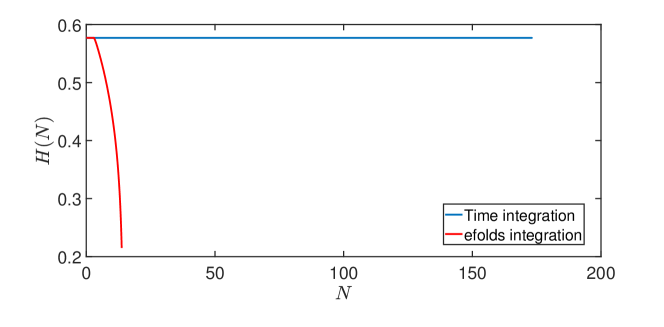
Fig. 4.1: While analytic integration over efolds, cosmic or conformal time are equivalent, integration over conformal time is nigh impossible due to tendancy toward an ’exploding’ solution. Numerical integration over efolds or cosmic time usually give near identical results, but in some cases, as shown above they diverge considerably. To be perfectly clear, we do not state with absolute confidence that one is better than the other, simply that they may differ. Since neither cosmic time nor efold number are strictly observables, and we are unable to run an experiment to validate one version over the other it is hard to prefer one over the other. However we contend that this does merit some additional discussion within the computational cosmology community. Further differences, especially in potentials which sport a plateau, were discussed by Coone, Roest, and Vennin Coone:2015fha.
-
(b)
At the time of writing the INSANE package, no computing language had both an embedded symbolic math capability as well as good numerical solvers (the one exception to this is Mathematica which was, at the time, opaque to ‘under-the-hood’ scrutiny). Thus by writing this package using Python, we were able to include fully symbolic parsers.
4.1 Code architecture
The code is organized into two main components each with its routines and sub-routines. The chosen computing language was Python, since at the time it was the only language to support both numerical integration and symbolic math, along with an object-oriented-programming (OOP) paradigm. The OOP compatibility was paramount for the construction of code that is reusable and can accept any inflationary potential. Initially, the plan was to have the code accept any physical action along with any underlying metric, construct the appropriate Friedmann equations and then develop and solve the background and MS equations to yield the full PPS. However, since we decided on studying small field scalar potential models, this was deemed a wild overshoot and was relegated to possible future projects. Additionally, the inclusion of a Boltzman code, pyCAMB Lewis:1999bs, and a sky-map realization, HEALpy Gorski:2004by, is a recent implementation and as such have yet to be fully debugged.
4.1.1 Background evolution
This part of the code is given several parameters, for the evaluation of the background geometry given an inflationary potential. The equations of background evolution are given by the Friedmann equation, along with the Klein-Gordon for the inflaton field:
| (4.7) |
It is implicitly assumed that we are dealing with a FRW metric such that the scale factor can be gleaned directly from knowing . The parameters supplied are the following:
| Param. | Type | Default value | Description |
| V0 | double | the scalar potential at | |
| H0 | double | , Initial Hubble parameter | |
| phi0 | double | Initial value | |
| phidot0 | double | Initial value | |
| efolds | double | Number of efolds to simulate | |
| in the CMB window | |||
| efoldsAgo | double | 60 | Number of efolds in the simulated |
| inflation, minimum is 50 | |||
| Tprecision | double | 0.01 | Precision of time integration |
| for the Background geometry solver |
Potential
The inflationary potential that is supplied to the simulator can be in the form of a single variable potential, for instance, with some set of predefined , or a set of numerical coefficients such that the potential is a finite polynomial representation of some function:
| (4.8) |
Currently, the code accepts polynomials up to degree 5, degree 6 and more polynomials should be inserted as symbolic functions. The code then parses this expression, and decides whether to manufacture a lookup table as a stand-in for the potential at different values of , or use the potential as is, in the case of a polynomial representation.
Background Geometry
The Background geometry solver class receives the potential, parses it, and integrates the Friedmann equations of the zero-order scalar field . The design choice was to use the cosmic time equations, since the conformal solution explodes to infinity faster than exponentially, close to the end of inflation, which makes the integration step go down to zero. Thus using an integration scheme that can handle exponential integration over a large stretch of time was called for. The equations we integrate are given by:
H_rhs=(-1/float(2*Mpl**2))*phidot**2
phi_rhs=phidot
phidot_rhs=-3*H*phidot -vd  ,
where the rhs suffix means this is the coordinate derivative such that phi_rhs means , and vd is the numerical equivalent of .
In order to solve the background equations, initial values must be supplied. The BackgroundGeometry initiator method __init__ takes the following arguments:
Ψ
(l1=0,l2=0,l3=0,l4=0,l5=0,Hubble0=None,Phi0=None,PhiEnd=1,
Phidot0=None,Tprecision=0.01,endTime=200,Planck_Mass=1,
physical=True,selfCheck=False,poly=True,
Pot=(sym.Symbol(’x’))**0,mode=’silent’) ,
where l1 through l5 are a degree 5 polynomial coefficients such that . Hubble0,Phi0,Phidot0 are initial values for correspondingly. We can set the integration precision as well as several other quantities. In general in the Python syntax, where an equality sign appears, this is the default value, such that Tprecision=0.01 means the integration step is ‘seconds’, unless otherwise specified.
4.1.2 Cosmic Perturbation
As outlined in 1.5.2, the equations for modes of scalar perturbation are given by the set of MS equations (1.155), one for each -mode. In order to solve these, we first need to construct the pump field (1.33). The Background solver contains, among others, the fields in Table 4.2, which are used to construct the pump field . One important note - the field a in the BackgrounGeometry class denotes instead of , and needs to be exponentiated before construction of .
| Class field | type | Description |
|---|---|---|
| BG.a | ndarray(float128) | Instead of , this is |
| or equivalently the number of efolds | ||
| from the start of inflation. | ||
| BG.phi | ndarray(float128) | |
| BG.phidot | ndarray(float128) | |
| BG.H | ndarray(float128) |
After constructing the pump field it is possible now to solve the MS equation for each mode.
The Mukhanov-Sasaki solver
The class responsible for solving the MS equations for each mode, and construct the PPS is MsSolver. In general, the class is fed the quantities at initiation as well as other parameters. MsSolver then splines everything, finds the analytic expressions for the observables in several approximations (Eqs. (1.179,1.180,1.184,1.196, etc.)), and finds the CMB point by calculating a user-specified number of efolds back from the end of inflation. It then finds the corresponding to the CMB point. This is done by finding the pump field value at , by setting the time-dependent frequency in Eq. (1.157) . we thus find the number which is just now entering the horizon and call it . This corresponds to the scale of the universe and is, therefore, the physical . If we are interested in physical inflation, this scale will be the default pivot scale, unless some other scale was set as the pivot scale. A preparatory phase is immediately initiated after the class is built, in which an interpolation table is created for the pump field and all quantities needed for a solution of the MS equation to arbitrary precision. The precision is predefined by the user, usually due to memory and running time considerations vs. precision demands. The solver then proceeds to integrate the MS equation for each -mode, build a two variable function which is a stack of eigenfunctions along the axis. The solver finally builds the quantity
| (4.9) |
and evaluates this function at a time much later than the freeze-out time of the last mode of interest, to yield:
| (4.10) |
This concludes the calculation phase, after which we have an array of -numbers, corresponding to the -modes, and the PPS as a function of these -numbers. The analysis phase now begins, in which we assign the pivot-scale specified. We first reassign to the correct physical scale:
Ψk=(k/k0)*1.2*10**(-4) .
If the user specified a pivot scale , we further assign:
Ψk=pivotScale*k/(1.2*10**(-4)) .
This effectively sets the point around which we will Taylor expand as the pivot scale. The analysis phase continues by fitting the power spectrum with a polynomial fit around the pivot scale. The polynomial fit degree starts at , i.e. linear fitting, and if the SSE value is over a set threshold, the degree is increased. This is done until the SSE is lower than the set threshold or the polynomial degree reaches 20. We assume that if polynomial of degree 20 does not accurately fit the power spectrum, we either have some error along the way, or we are describing a manifestly non-physical scenario.
In order to correctly initialize the MsSolver class the following input needs to be supplied:
Ψ
(a,H,phi,phidot,t,epsilon,eta,xisq,Vd4V,Vd5V,V,
eh,delh,pp,Tprecision=0.0064,Kprecision=15,
log=True,pivotK=0.05,efoldsAgo=60,efoldsNum=8,
check=False,physical=True,mode=’aprox’) ,
where a,H,phi,phidot,t,epsilon,eta,xisq,Vd4V,Vd5V,V,eh,delh,pp are all fields manufactured in the BackgroundGeometry class, and held as internal fields within it. Tprecision and Kprecision are precision parameters, for integration time-step, and for the number of -modes to solve and include in the construction of the PPS. If log=True the code draws -numbers such that the distribution of ’s will be uniform in a log-log scale, to have equal fidelity across the CMB window. pivotK,efoldsAgo,efoldsNum are the pivot scale, number of efolds to consider in the inflation as ‘visible’ inflation, and the number of efolds in the window to analyse as the CMB window, correspondingly. We allow for non-physical inflationary scenarios in which slow-roll is not held along the entire CMB window, in which case we will set physical=False. Finally we consider the exact number of inflationary efolds by setting mode=’exact’, otherwise, setting mode=’aprox’ means the CMB point will be set at . The difference between both cases is very slight, but may be of import in some cases.
4.1.3 Usage
In order to correctly use INSANE, one must specify several arguments. These arguments are conveniently edited in the params.in file. The full file along with example inputs is given in Appendix B.
4.1.4 Benchmarking
Several tests are now in order to asses the voracity of this code. We first test the code against the only known relevant analytical solution - the power law inflation111There are other analytical solutions (c.f. Martin:2000ei) but they are not relevant since they produce a very blue tilt, not in the vicinity of the observable regime..
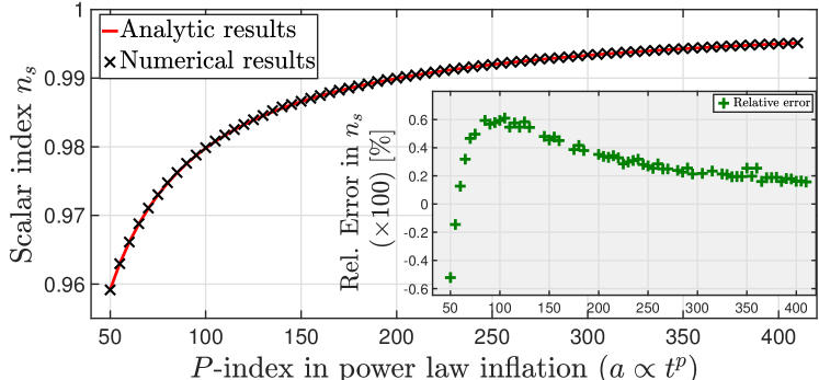
The power law case
The power law inflation is the case where the Hubble parameter scales as during inflation. The scalar potential that results in such a case is given by:
| (4.11) |
in which is the same as the power law index. The resultant scalar index of such an inflationary scenario is given by:
| (4.12) |
and is scale independent, such that the index running vanishes by definition. We have run the INSANE code against these scenarios to compare analytic and numeric solutions. The results are shown in Fig. 4.2, and reveal an agreement between analytical and numerical analysis to a relative error of order . In evaluating the fidelity of there is an intrinsic problem since in the analytic case it vanishes by definition. Thus no intrinsic scale is available for us to relate to. We, therefore, took the heuristic approach of assessing . If , as recovered by the code, is lower than , we are satisfied that the code yields a correct .
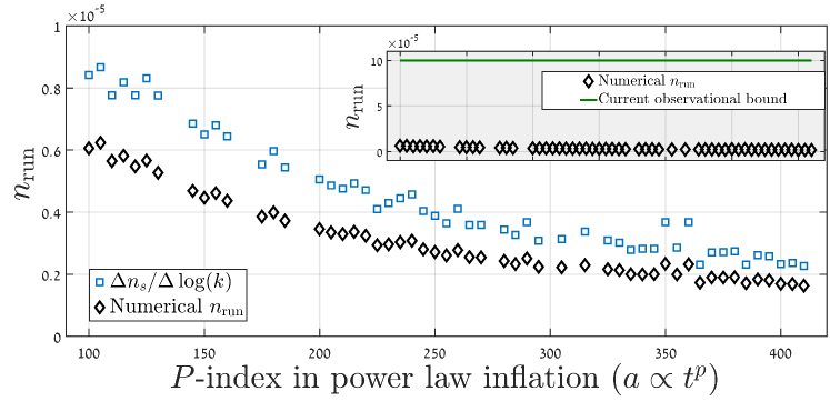
We find that the values recovered by the numerical calculation are always below the numerical error in divided by the overall . We take this as a sign that the recovered is at the level of numerical error, thus equivalent to a vanishing . Fig. 4.3 shows these findings. Additionally, we show the current observational threshold of .
The quadratic case
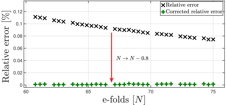
As we aim to study models that produce slow-roll parameters which are time-dependent, we need to check the precision of the numerical code against such models. Consequently, we tested the accuracy of our calculations for quadratic potentials of the type
| (4.13) |
In these cases, the analytic expression for the scalar index is given by,
| (4.14) |
Here is the number of efolds and is the same as in (1.179). Fig. 4.4 presents the results of this study, as relative errors between precise calculations and the SL analytic expressions. These results are accurate to . However, there is a systematic error that is traced back to the inaccuracy of the approximation:
| (4.15) |
A shift is sufficient to reduce the systematic error such that the relative error is of the order of . Additional types of simple potentials, which yield time-dependent slow-roll parameters were also studied. In all cases, the relative error between calculated results and the traditional SL expression Eq. (5.20) is bounded from above by . Furthermore, a more careful analytical treatment leads to better accuracy, bounded from above by about 0.02% relative error. Additionally, we were able to recover the “Cosmic ring” phenomenon, that is the PPS response to a step function in the potential. This response feature in the PPS was first studied in Adams:2001vc.
We take all these results as a strong indication of sufficient accuracy of our calculations.
4.2 Improvements - Teaching a PC some physics
In order to speed up the calculation, and enable the study of a class of inflationary potentials rather than a solitary example, some adaptations of the code were called for. The most crucial and time-consuming element of calculating the power spectrum is the numerical integration of the different -modes that make up the PPS. We, therefore, identified several mechanisms that, while technically might be interesting, produce little to no effect in the context of yielding the PPS.
4.2.1 Finding the mode ‘freeze-out’ point
The first and most influential improvement was achieved by using the physical understanding that each mode of quantum oscillation ‘freezes out’ of the horizon at some point in its evolution. That is, at some point of the inflationary evolution the light horizon becomes smaller than the mode’s wavelength. If we take the viewpoint of the classical harmonic oscillator such that
| (4.16) |
with , which at some point becomes negative, it is immediately apparent that becomes purely imaginary around
| (4.17) |
And so, since we care only about the modes after the freeze-out time, we can in theory start the integration approximately around the freeze-out time of each mode. We call this ’finding the "knee"’ since the modes oscillate around an overall similar amplitude all throughout their evolution inside the horizon, but around the freeze-out time their amplitude begins to grow quasi-exponentially and the phase becomes locked. Thus if we look at the square of the eigenfunction the ’knee’ for each mode is approximately at the freeze-out point.
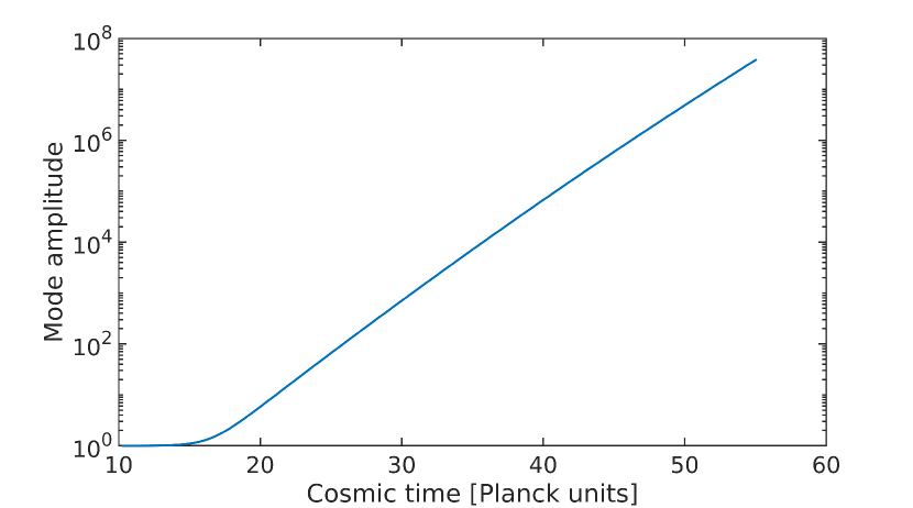
4.2.2 Forgetting the phase
While the former subsection discussed the amplitude, we are also interested in the phase. Since we are dealing with TDHO the phase and amplitude are coupled to some degree. In theory, then, one cannot simply forget about the phase and integrate the amplitude alone. In fact, this is a common mistake that is done in most numerical schemes to date. However, it is true that the phase gets "locked" when the mode is frozen out of the horizon. In this case, the information of the phase does not evolve any more and provided we know the amplitude and phase at the freeze-out time we no longer have to take them into account when integrating the mode. Several efolds prior to the freeze-out scale of a mode the associated frequency satisfies , thus the mode oscillates wildly, and in effect the mode ’forgets’ the initial phase. This is an oversimplification since some of this information is still carried in the evolution if the amplitude. Be that as it may, the longer prior to the freeze-out time we start the integration this added correction to the amplitude becomes negligible.
4.2.3 Pre-Integration
With the combination of these two last insights, it is evident that it is enough to start the numerical integration some 2.5 to 3.5 efolds prior to the freeze-out time for each mode. In this fashion we both truncate the runtime for each mode while keeping the correct information. Another issue that is critical from which it is apparent that we should perform integration several efolds before freeze-out is that of initial conditions. The Bunch-Davies initial conditions are applicable for each mode only deep into the oscillatory phase. These conditions contain critical information, as they contain the seed amplitude which will define the evolution and ultimately the dependence of the PPS.
Chapter 5 Fresh eyes on
5.1 The discrepancy
One of the surprising results found during our studies is that a fully numerical treatment of inflation yields different results, from an analytical perturbative treatment. This should not surprise us, as the usual way perturbation theory is used, is by removing sub-leading terms of some order. However, the underlying assumption of this practice is that the sub-leading discarded terms issue tiny corrections relative to the leading terms. This might not always be true. Furthermore, the non-perturbed case should be chosen wisely, such that there is a natural scale to perturb over.
The surprising aspect is not the difference itself, but the scope of the difference. We show that in the type of models we study the relative difference in is usually well over . We have also seen that even in the case of ’well behaved’ models there is a marked difference in between analytical and numerical treatment.
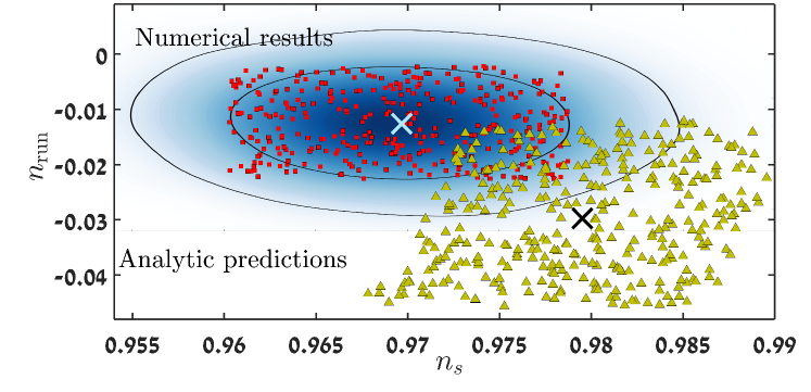
5.1.1 Slow-roll hierarchy
In potentials which are so-called large field models, i.e. where inflation occurs over , the number of efolds per field excursion , and is usually taken to be monotonously decreasing. The Lyth bound Lyth:1996im, originally states that in accordance with current observations, there is a bound on the field excursion that creates the observable scales in the CMB. Several works since (c.f. Efstathiou:2005tq) have expanded the Lyth bound to include the entire span of the inflationary potential, up to the end of inflation. However, these works always assume a generally monotonous . This yields a natural hierarchy for the slow-roll parameters. The relations between slow-roll and their temporal derivatives is also suggestive of this:
| (5.1) | |||
| (5.2) |
and this relationship continues where in general Gong:2001he:
| (5.3) | ||||
| (5.4) |
However, this relation does not always hold. When is not monotonous, the derivative can be high enough to break the hierarchy. This is the case with the small field models we study. While the original Lyth bound still apply in these cases, the extended version is broken.
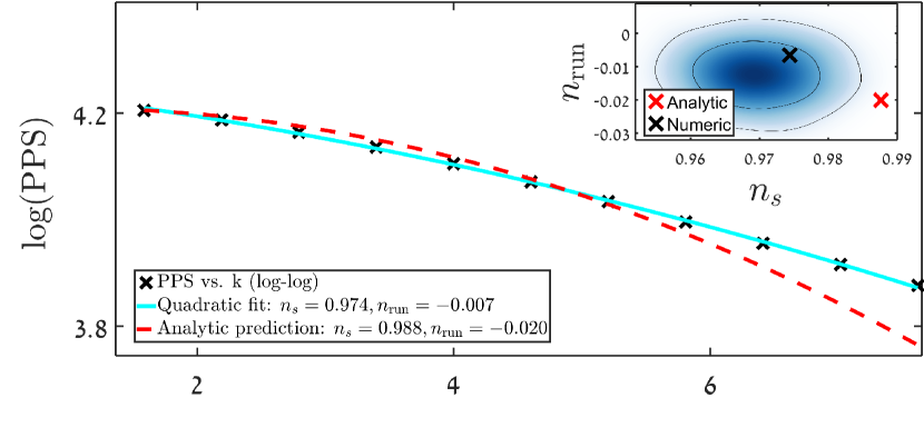
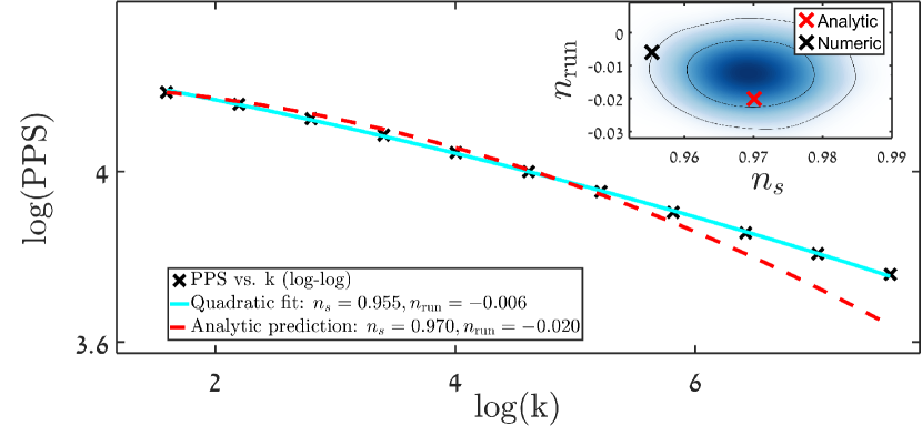
5.1.2 Another degree of separation - slow-roll in potential language
The original formulation that ties the slow-roll parameters to the characteristics of the PPS uses the slow-roll parameters per their Taylor expansion definition. In Stewart:1993bc it was shown, that assuming is small, where , the following relations apply:
| (5.11) |
where the potential derivative terms are given by:
| (5.12) |
As was previously shown in section 1.5 these relations are exact at the end of inflation as well as in the case of an exponential potential, that corresponds to the pure dS case. The way to derive these relations is the following. We begin with the set of exact relations:
| (5.13) | |||
| (5.14) | |||
| (5.15) |
and the definitions for , and . We now derive the Klein-Gordon equation with regards to cosmic time to yield:
| (5.16) |
proceeding to substitute the original KG equation for , and setting the highest derivative , we get the following:
| (5.17) |
where applying the relations in (5.15,5.13), yields the desired term. This procedure can be followed to arbitrary order; derive (5.14) w.r.t , times and (5.15) times. Set the highest derivative , substitute iteratively the previous derived relations and , until we get a term that is a function of . Assign the slow-roll parameter definitions where applicable, and arrange the potential terms to combinations of (5.12), and a new term will arise of the form:
| (5.18) |
A word of caution though, in order for complete equality between the formulation of the slow-roll parameters and the potential and derivatives formulation to be exact, the infinite tower of equations should be developed. This is the analogue of a Taylor expansion exactly agreeing with the underlying function only in the case of an infinite Taylor series. It can be shown that the remainder takes the form of
| (5.19) |
Since a small does not assure us of a substantially smaller , there is no real way of assessing this remainder without either having a fully analytical expression for , or a numerical value of through the entirety of the CMB window. This is unfortunate since it means there is no assurance of these relations except in the case of either extremely controlled slow-roll or fully analytical cases. Of the latter there is only one case that approximates observed values, which is the pure dS case. We have no reason to believe a-priori that the former case is more likely than any other.
| precise | analytic | precise | analytic | Fit error | ||
| () | ||||||
5.1.3 Does the formulation work?
The Lyth-Riotto formulation in Lyth:1998xn for the running of the scalar index, , is derived by using the analytical expression for , up to second order:
| (5.20) |
with , where is the Euler-Mascheroni constant. By deriving Eq.(5.20) with respect to , keeping terms up to second order in slow-roll parameters the term for in Lyth:1998xn is given: 111Note that in Lyth:1998xn our corresponds to
| (5.21) |
However, the original expression for the scalar index was derived by Stewart:1993bc for the exponential inflationary potential, which yields a strictly linear . Since has no natural scale, even the slightest perturbation around it may be considered large. This means that this perturbative formulation for is by definition impossible. In addition, almost all such formulations assume an unbroken hierarchy of slow-roll parameters. This assumption is based on the faulty logic of:
| (5.22) |
This assumption is only correct if both and are strictly smooth, non-oscillatory, and the relation holds for a long interval on the axis. These conditions are in no way guaranteed, especially since the natural eigenfunctions of the PPS are Hankel functions which are by nature oscillatory. Furthermore, even a slight step-like feature in the inflationary potential yields a non-proportional response of an oscillatory nature. In fact, the motivation for looking at the numerical results for as compared to analytical predictions first came up from looking at the numerical results for the index running , as compared to the analytical expression in Eq. (5.21). We found that the disparity between these can be of the order of sometimes, and there doesn’t seem to be any consistency in the comparison between analytic predictions and numerical results.
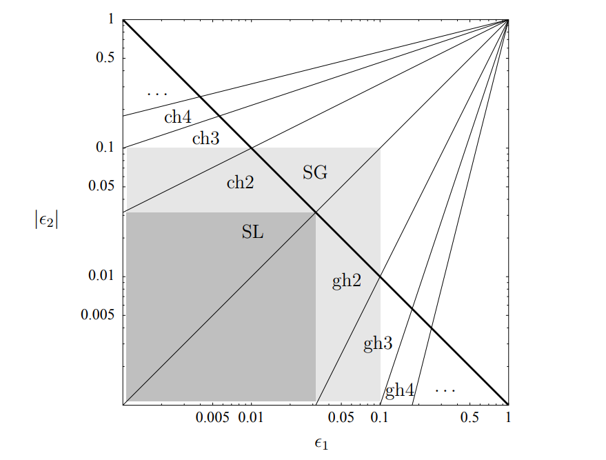
5.2 A Green’s function approach
There are two analytic approaches we discuss, the first is the so-called ’raw’ Green’s function approach in which we present the Green’s function for inflation. The second is to use the same mathematical ’trick’ used by Stewart in Gong:2001he, and use the adjusted Green’s function.
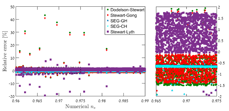
Raw Green’s function approach
Over the years some attempts have been made to analytically derive the PPS in a more accurate way. The most promising of which was the Green’s function approach along with perturbative corrections. The Green’s function for scalar field driven dS inflation is given by:
| (5.28) |
where is the first Hankel function of order . In order to derive the correct eigenfunctions given some other inflationary potential, one decomposes the pump field term to a dS pump field term + a correction term
| (5.29) |
In this manner, we get the perturbed eigenfunction by:
| (5.30) |
where is the set of dS k-eigenfunctions which are in general a linear combination of spherical Hankel functions of the first and second kind.
This means that there are closed-form analytical solutions only for a restrictive set of input functions, as were evaluated for instance in Dvorkin:2009ne.
In the general case, there are no known analytic solutions to the problem of inflation with a scalar inflationary potential. Furthermore, the perturbative approach was not probed sufficiently for its validity limits.
One point of interest is that the preferred eigenfunction space for evaluating the PPS and its features is the Bessle function one. This is also demonstrated in Adams:2001vc, where a step function feature in the potential has a compressed Bessel function response over the baseline PPS. Since the step function creates a ’double delta’-like feature in the pump field, one can consider the compressed Bessel response to be the natural decomposition basis of the PPS.
Adjusted Green’s function
In Gong:2001he the author used a mathematical ’trick’ where we define:
| (5.34) |
along with the ansatz:
| (5.35) |
In this approach the eigenfunctions are simpler to integrate perturbatively since the equation takes the form:
| (5.36) |
with a homogeneous solution of
| (5.37) |
This approach amount to the following solution:
| (5.38) |
in which is the small perturbation parameter, is some convenient time around horizon crossing, and is the generalized factorial Gamma function. While this formulation is sound, several assumptions are made. These include the first order evaluation of to be small and the validity and smoothness of the function . It was shown in Dvorkin:2009ne, that in this case, several iterations are needed to achieve a less than accuracy as compared to the exact solution. Thus this approach serves at best as a good guideline. However, in the age of precision cosmology, this is not enough.
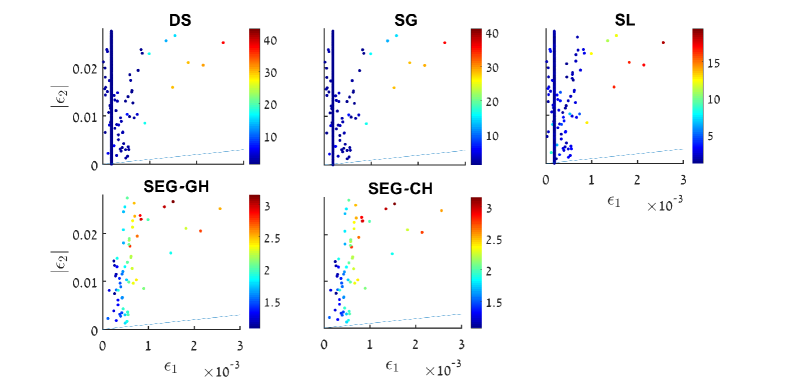
5.2.1 Possible explanations of the source of deviation between precise results and analytical estimates.
From the discussion in section 1.7 , one can easily see that the definition of , is potentially the most significant discrepancy. The effect of this change in definition is an error of less than about .
Table 5.2 contains three examples of potentials. Two yield observables that are within acceptable limits and a third shows an excluded precise result with an allowed analytic prediction. Examples such as these are used to study the origin of discrepancy.
| Ex. no. | ||||||
|---|---|---|---|---|---|---|
| 1 | ||||||
| 2 | ||||||
| 3 |
The differences between the slow-roll parameters defined via the potential vs. their definition in terms of time derivatives are also discussed in section 1.7. We have found, that in the degree 5 polynomial potentials that were studied, small but significant departures from the relations in Eq. (5.12) are detected. For instance and at the time when is evaluated. Table 5.3 contains values of the three quantities as precisely calculated and analytically approximated, for three potentials of the degree 5 polynomial class. Table 5.4 contains the scalar index for the corresponding potentials (examples 1,2 and 3).
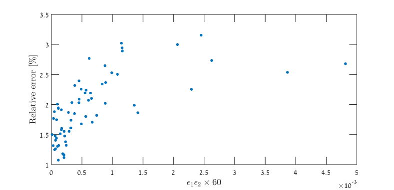
| Ex. no. | Quantity | slow-roll value | pot. der. value |
|---|---|---|---|
| 1 | |||
| 2 | |||
| 3 | |||
The overall effect of this discrepancy can sometimes amount to a error towards higher values.
Finally, there is also a significant difference in the derivatives of and , being in the SL formulation:
| (5.39) |
where time dependency of the slow-roll parameters is neglected. This difference is mainly due to neglecting the term in the definition of . This yields a difference in the derivative terms of the order of , which in turn is responsible for a difference in of the order of . Using instead of the full term tends to drive the resulting downwards.
The tendencies of the two aforementioned errors are opposite, and so they might sometimes cancel each other. This makes it possible to get an accurate result using the standard SL expression for a specific potential, but studying a collection of such potentials reveals the incomplete nature of this cancellation.
Table 5.4 shows the different results using different methods of deriving the scalar index. We use three different analytical methods: (1) Eq. (1.179) - The SL original method, extracting a term for the scalar index as a function of the potential and its derivatives, (2) Eq. (1.170) - The SL original method, but not relating slow-roll quantities to potential and derivatives, and (3) Using the same methods as the SL analysis, with the definition for as in Eqs. (1.164,1.168,1.170). From this analysis, it seems the origin of the most significant error is the inaccurate relations between slow-roll parameters and their potential and derivatives counterparts. Second in significance is the definition of with the full expression, along with the proper derivation of . The evaluation of is off by and the difference between and yields a correction of the order of .
There might be additional factors that stem from the temporal dependence of in the MS equation. However, these mostly affect the running of the spectral index, and are harder to estimate accurately.
Taking these approximations into account, lowers the discrepancy to the order of , in a consistent manner. Another possible explanation is that the time-dependence in (1.167), modifies the corresponding to . This could lead to modified solutions for the MS equation. An example of this phenomenon is given in Martin:2000ei, where the Hankel functions were replaced by the Whittaker functions (albeit these models are observationally excluded). It is worth mentioning that this avenue was studied analytically by Dodelson & Stewart Stewart:2001cd; Dodelson:2001sh. They derived an expression for the scalar index in cases where the slow-roll hierarchy breaks down. However, this analysis was not checked numerically. Additional derivation attempts aiming at yielding better precision analytical expression for the scalar index were made in Gong:2001he; Schwarz:2001vv. Specifically Schwarz:2001vv supplies an analysis of the predicted level of accuracy as a function of the horizon flow functions and , in figure 5.3. The different approximation schemes were put to the numerical test in the context of our models. Figure 5.4 shows that all methods of approximation yield results varying in accuracy and precision levels, it also shows however that the SEG approximation is the best candidate to improve on since on average they yield errors of less than . Studying results where relative errors in are over , for each expression and locating it on the diagram in figure 5.5 reveals that the analysis offered in Schwarz:2001vv is not completely applicable to our models. Figure 5.6 shows that for the models studied, even though the conditions outlined in Schwarz:2001vv are met, and for , the relative error between numerical result and SEG-CH expression can be above .
| Ex. no. | Num. value | Eq. (1.179) | Eq. (1.170) | Eq. (1.164,1.168,1.170) | |
|---|---|---|---|---|---|
| 1 | |||||
| rel. error | /NA | ||||
| 2 | |||||
| rel. error | /NA | ||||
| 3 | |||||
| rel. error | /NA |
So what is it good for?
Absolutely nothing. This whole exercise in relating PPS directly to the inflationary potential and derivative was supposed to yield two advantages:
-
1.
To be able to compute the PPS directly from the inflationary potential in a fast way. This is partially achieved with Dvorkin:2009ne. However in the age of High-Performance-Computing (HPC), clusters and Graphic-Processor-Unit (GPU) based computing, the advantage of this approach is marginal at best.
-
2.
To be able to solve the inverse problem: Given a PPS as recovered from observations to be able to directly calculate the inflationary potential. This notion has been annihilated by the above analysis since it becomes evident that a direct connection through etc. is not valid, and even if possible, deconvolving the inflationary potential via the approach in Dvorkin:2009ne would be extremely costly in time and resources.
Chapter 6 Results
6.0.1 Models with
In this section, we present the results of evaluating cosmological parameters for many small field models. In Fig. 6.1 we show an example for which we calculate and for about 1100 models with a fixed scalar to tensor ratio . The results are shown on a joint probability graph with the contours that are the probability estimators as yielded by a CosmoMC Lewis:2002ah CDM +index running model run, with the most recent Bicep & Planck data (including WMAP 9-year mission) Ade:2015tva.
The reason for initially choosing the value of (and not a higher value, for example, ) was the following. We discovered that as we increased the values of , the inflaton potentials needed to be more complicated and additional parameters were required. Also, we encountered several technical difficulties which we were able to resolve for the lower values of . Solving these difficulties and constructing a reliable framework for numerical calculations of the CMB observables was an essential step towards building models with higher values of .
We allow the values of to vary quite substantially, rather than restrict them to the narrow range that is allowed by the data. Our idea is that when and are free to vary, the constraints on are relaxed in a significant way. The reason is that there is some degeneracy among the parameters. This is validated in the preliminary analysis that we present here. In addition, despite the fact that some models have yielded an almost flat (and some even a blue) and therefore are in conflict with the data, we found their analysis useful because insight regarding the departure of precisely calculated results from what the analytic SL term (1.179) predicts was gained, as was discussed in chapter 5.
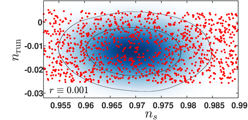
Evaluating cosmological parameters for fixed
The plane was covered with models which yield a fixed value of . The cosmological parameters of some 3500 potentials were calculated. Fig. 6.1 shows cosmological parameters of 1100 models. A significant number of the models yield values of and within the and likelihood region. The most probable value for . This is within the CL Planck results, with or without including high- polarization data. The third coefficient values are given by , which is in better agreement with the result without high- data. However the 2015 Planck analysis Ade:2015lrj sets which might bias the results slightly. In the 2013 analysis Planck:2013jfk this was not done, and our results agree with their analyses, including our values for . Additional factors that contribute to the difference in analyses are the approximate connection between Hubble flow functions and the potential derivative quantities . An interesting feature of these models is the departure of precisely calculated results from what the analytic SL expression (1.179) predicts, as discussed in chapter 5. It might be possible to cover the allowed region with models with a higher scalar-to-tensor ratio. However, the treatment of models which yield higher is more complex since, by increasing , one is forced to consider a larger range CMB region. The CMB region (see Fig. 2.1) is roughly 3 times larger in for models with , thus it will typically result in a running of running of the power spectrum.
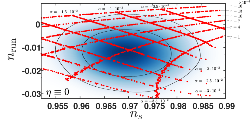
Evaluating cosmological parameters for fixed
The effects of varying on the resulting power spectrum were studied. In order to do this was set to for simplicity, and the plane was covered with models of varying and . Fig. 6.2 shows the results of this study.
Notice that the effect of varying both and on the changes in the value of is more pronounced than expected. Usually when one expects to first order to be and thus . At second order, we expect to be and thus , whereas in this case, the change in is of the order of . A possible explanation to this phenomenon is a discrepancy between the analytic predictions made using (1.179) and the precise calculations (see chapter 5).
6.1 6th degree models with
We apply the methods discussed in Chapter 3.0.1 to the degree six polynomial inflationary potentials that yield . We calculate the most likely coefficients and extract the resulting most likely polynomial inflationary potential. The PPS resulting from this inflationary potential is then calculated in order to confirm that the most likely coefficients reconstruct the most likely observables.
6.1.1 Results for degree six polynomials that yield
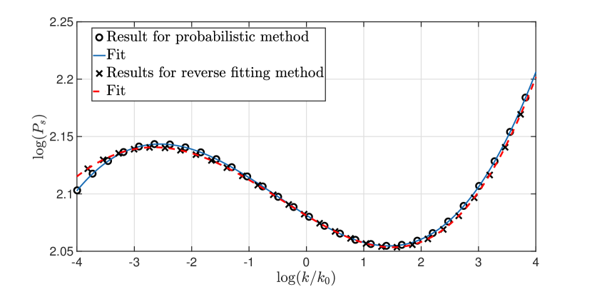
In Fig. 3.1 we showed a cover for the joint likelihood map of , of about potentials with . The cover is approximately uniform, thus we were able to assign likelihoods to every potential we study, as previously discussed.
By a process of marginalization, as discussed in Section 3.0.1, we extract the most likely coefficients, which yield the likeliest observables. This process is represented graphically in Fig. 3.2. The results are shown in Table 6.2 and the PPS reconstruction is shown in Fig 6.3. The advantage of this method is that it also determines the deviation from the average value. This can be used as an indicator for the level of tuning that is required to construct the most likely small field model. A discussion of tuning in field theoretic models can be found in Barbieri:1987fn, as well as in Ellis:1986yg and Fowlie:2014xha. In most cases, the tuning level can be viewed as simply , which in this case are given by for respectively. The width of the Gaussian fits for are respectively. These widths represent the effective area in parameter space that yields observables within the CL. Which is another measure of the tuning required in the degree 6 polynomial models.
Recalculating the CMB observables that this most likely model yields, we find . These values are very close to the most likely values found from the previously discussed MCMC analysis of the BICEP2+Planck data. The resulting scalar index fits the most likely value in Table 3.1 exactly, while and deviate from these values by no more than . We found that this is a relic of the binning method. Adding more models to the simulated data and refining the binning process results in even better proximity to the desired values.
Using the method of multinomial evaluation (3.0.1), we found the multinomial coefficients for each of the model degrees of freedom. For instance, for we have:
| (6.7) |
Since , and and are of the order of , the above result suggests that is primarily dominated by . Similarly, we have found that is dominated by a linear combination of , and , and is primarily dominated by . This method yields the most likely CMB observables with comparable accuracy to the previous method upon recalculation: .
6.1.2 Most likely potentials
| Observable | Recalculated | |
|---|---|---|
| Probabilistic Method | Multi-fit | |
Since is better constrained, we opt for the analysis that yields a more precise value of . The leading degree 6 polynomial which yields at the proper pivot scale, is thus given by:
| (6.8) |
Upon initial investigation, it seems these models produce a relatively flat tensor power spectrum. This might motivate future research of the tensor power spectrum predictions and constraints.
6.1.3 Observable dependence
| Gaussian extraction | Multinomial fit | ||
|---|---|---|---|
| (average) | (standard deviation) | value | |
An interesting finding is an inter-dependence of the three observables . For models that yield , there is a quadratic relation between the observables, such that . It should be stressed that this is a phenomenon associated with the models and not with the observational data. This is supported by the small paired-covariance found in Cabass:2016ldu, implying weak dependence among observables in the data itself.
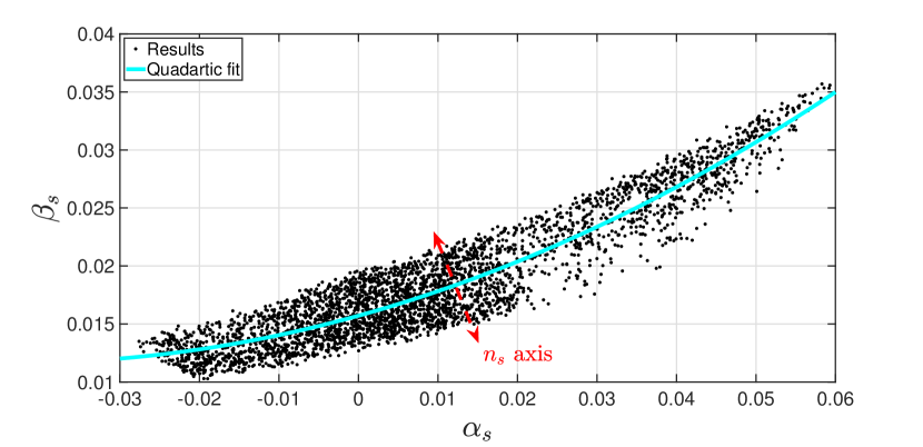
One might think that the previous findings in (Ade:2015xua, Figure 23) indicate that and are dependent. However, the graph shows a dependence between and which is the scalar index evaluated at . Taking some initial evaluated at , it follows that evaluated at some other scale depends on the index running . Indeed, when one examines the color coding in (Ade:2015xua, Figure 23), which represents at the pivot scale, it is clear that and are independent.
6.2 6th degree models with
6.2.1 Methods
We analyse the most recently available observational data Aghanim:2018eyx by using CosmoMC Lewis:2002ah, extracting the likelihood curves of the scalar index, its running and the running of running, respectively. We then simulate a large number of inflationary models with polynomial potentials and calculate the primordial power spectrum (PPS) observables , , , that they predict. Each simulated potential is assigned a likelihood by the combined likelihood of the observables that it yields, as discussed in detail in Wolfson:2018lel. We restrict the models that we consider to those predicting a power spectrum that can be fitted well by a degree 3 polynomial. This corresponds to the scalar index , the index running , and the running of running . We do that by fitting the PPS and evaluating the fitting error
| (6.9) |
where is the fitting curve. The threshold for considering a specific model in our analysis is .
An additional complication arises due to the higher amount of tuning that is required for these models. The coefficient is fixed as BenDayan:2009kv, so when the value of is higher, then at the CMB point has a larger magnitude. This has the effect of decreasing the number of e-folds generated per field excursion interval. If is increased to , then is decreased by a factor close to the CMB point. Since the first 8 or so e-folds of inflation are fairly constrained by observations, the amount of freedom in constructing the potential is reduced. It follows that either greater tuning is required to construct valid potentials, or one should consider a higher degree polynomial as suggested in Hotchkiss:2011gz. Ultimately the choice is a matter of practical convenience. We opted for using degree 6 polynomials.
We employ two methods of retrieving the most likely polynomial potential. First, we extract by marginalisation the most likely coefficients . The other method amounts to performing a multinomial fitting of the coefficients as a function of the observables and then inserting the most likely observables to recover the corresponding coefficients. This method is explained in detail in Wolfson:2018lel.
The ‘most likely model’, is the model with a potential that generates the most likely CMB observables , as produced by the MCMC analysis of the most recent data available to date.
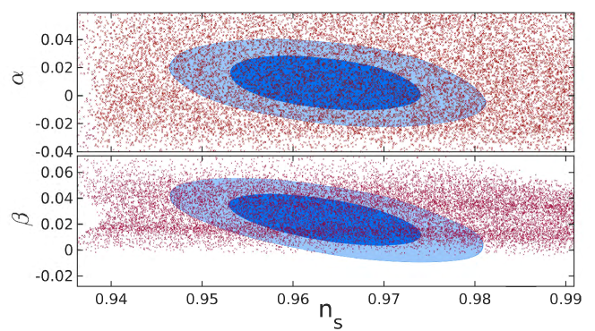
6.2.2 Results
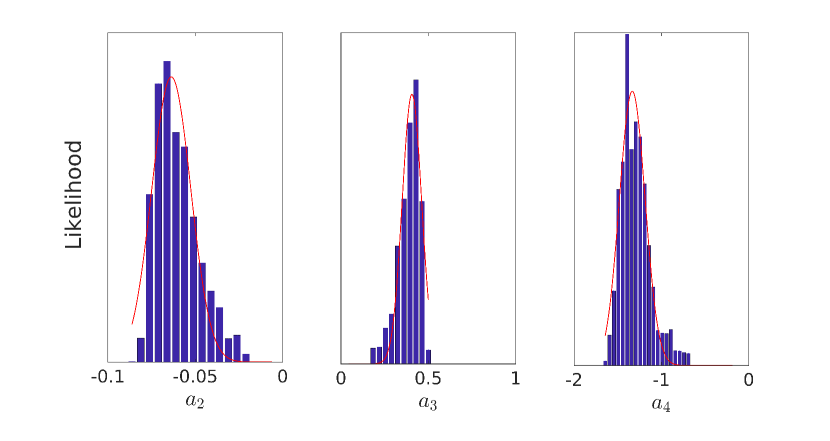
We produced many models that predict and, additionally, predict PPS observables within the likely values. A roughly uniform cover of both the and allowed values is shown in Fig. 6.5. This enables us to assign a likelihood to each simulated model, as discussed in detail in Wolfson:2016vyx; Wolfson:2018lel and in the methods section. Consequently, it is possible to perform a likelihood analysis of models. The results of this likelihood analysis is an approximately Gaussian distribution of the free coefficients as is shown in Fig. 6.6. Since the peaks of Gaussian fit (red line in Fig. 6.6) do not entirely coincide with the peaks of the distribution and the distribution tails are not symmetric, we conclude that the distribution has a significant skewness. The required tuning level is also evident from Fig. 6.6 and is given by . Using Gaussian analysis and taking into account the skewness, we recover the most likely coefficients, which yield the following degree six polynomial small field potential:
| (6.10) |
Due to the skewness of the distribution, the values obtained by the Gaussian fit deviate by a significant amount from the most likely values of the observables. For instance, as determined by the potential in (6.10) is which is about away from the most likely value. For this reason we use this method of analysis to evaluate the required tuning levels, whereas the most likely model is extracted by the multinomial fitting method.
Using the popular Stewart-Lyth (SL) theoretical values for and Stewart:1993bc; Lyth:1998xn as derived directly from the inflationary potential around the pivot scale, one finds values that deviate by a significant amount from the Planck values. The SL values correspond to a very blue power spectrum and large running,
| (6.11) | |||
This discrepancy, that was discussed in Wolfson:2016vyx, is related to the magnitude of for our class of models. When is smaller than in such models, the original model building procedure that relied on the SL values, which is outlined in BenDayan:2009kv, is valid and produces approximately the correct values of the observables. However, when values of are larger, one cannot trust the analytic SL estimates.
In Fig. 6.7 the power spectra generated by three inflationary models are shown. (1) A model with degree 5 polynomial potential that predicts ; (2) A model with degree 6 polynomial potential that predicts ; and finally (3) A model with degree 6 polynomial potential that predicts .
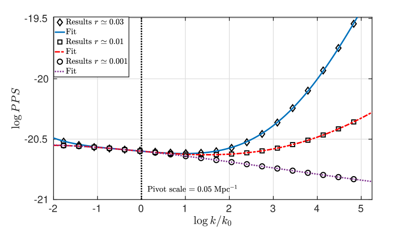
Representing each coefficient as a function of the observables and evaluating them at , leads to the following potential,
| (6.12) |
The values that this model predicts deviate from the most likely values by . However, the deviations are within the CL of all recent MCMC analyses.
Chapter 7 Conclusion
We have found that small field models of the degree 6 polynomial form can produce a significant GW signal at the level of while conforming to known CMB observables. We have further shown that analytic methods of evaluating the PPS in these models fail and a full numerical treatment is necessary. While the idea of these models is relatively new, it was first suggested almost ten years ago BenDayan:2009kv. However, our work was the first to put these models to the numerical test. Due to the failings of analytical methods of PPS evaluation, the model building technique originally suggested in BenDayan:2009kv was shown to be insufficient thus our work is the first to show the validity of these models. These models are gaining prominence among considered inflationary models, due to the swampland conjecture Garg:2018reu; Kehagias:2018uem; Ben-Dayan:2018mhe, that seem to favour small field models, over the large field variety.
In explicitly showing analytic approaches of evaluating the PPS to be insufficient in certain cases, we question the validity of such approximations in other cases as well. The discussion in section 5, also shows beyond a doubt that the second order Lyth-Riotto term for the index running given in Eq. (5.21) cannot, by definition, be correct. This means that all models previously analysed by using this expression are now in need of re-examination. This is further suggestive of a need for numerical reassessment of such codexes as Martin:2013tda, that heavily rely on such analytic tools.
Our initial hypothesis was that a degree 5 polynomial model with should be able to cover the full PPS observable phase space, as allowed by current CMB experiments. Our numerical analysis has disproved this hypothesis. Instead, we have shown that for full coverage of the observables parameter space with models which yield , either degree 6 polynomial models while allowing a running of running is necessary, or one must consider a degree 7 polynomial at least, such as in work done in Hotchkiss:2011gz. Be that as it may, full coverage is, in fact, possible by small field models with , which was the end goal of this research.
Whether one favours large field models or small field models, we have created the numerical tools that now seem to be indispensable in studying inflationary potentials in the age of precision cosmology. The limit of analytic tools have been known for a long time, we are by no means the first to point out this discrepancy and the possible theoretical pitfalls (cf. Wang:1997cw). However, we are the first to show the meaning of this disparity in actual results and their repercussions in terms of precision and model building. Our only hope is that future researchers find it necessary to evaluate their results numerically, at the high standard of precision we have now achieved.
* * *
If I may be so bold as to suggest my personal conclusions, one should aspire to make connections with people of different disciplines, in physics, and otherwise. This serves the purposes of mutual enrichment and comradery. Sometimes one needs the layperson for a set of fresh eyes on a problem. Sometimes an adversarial point of view is needed, to test new and somewhat ‘crazy’ ideas. But above all:
PHYSICISTS DO NOT GIVE UP!
Appendix A Derivation of Mukhanov-Sasaki equation
Deriving the equation of motion for in conformal time
In this section we will derive the equation of motion for the scalar field, and the perturbation thereof, in conformal-Newtonian gauge.
Using the conformal time metric we define:
| (A.1) |
Where is Minkowski’s metric.
We now take the action to be:
| (A.2) |
Varying in respect to we get:
| (A.3) | |||
Since we take the metric and the scalar field to be independent coordinates, and so we consider only the first term. Applying the symmetry of the metric we get:
| (A.4) |
Integrating by parts we are left with:
| (A.5) |
And the second term is just some constant, depending only on the boundary conditions, and not on any variational contribution, thus we are allowed to disregard it.
Thus we are left with:
| (A.6) | |||
| (A.7) |
which, up to now is a completely general result.
Plugging in the conformal metric we get:
| (A.8) |
And we are left with:
| (A.9) | |||
| (A.10) |
which reverts back to Eq.(1.90) if we consider a homogeneous, time dependant
However, this equation gives us additional information, as we will see in the continued derivation, since it contains the Laplacian term.
Now, looking back at Eq.(A.7), which, as stated is so far completely general, we want to apply perturbation theory approach and vary the coordinate slightly:
| (A.11) |
Doing this, is not enough, since there is an interplay between energy density (as affected by and functions thereof) and the metric. So we will also use a perturbed metric, and we will use the Conformal-Newtonian gauge in which:
| (A.12) |
Where as a rule the perturbation is very small compared to the zero order metric.
We will derive the equations using to give the most general result, and in the last possible moment, we will replace the abstract perturbation with a specific explicit one.
So, considering the perturbed quantities stated above we have:
| (A.13) | |||
Keeping only first order in perturbation (either in or in ) we arrive at:
| (A.14) | |||
We can simplify this a tiny bit by demanding the zero order term to vanish independently, to get:
| (A.15) | |||
Where the subscript means setting the metric perturbation to zero, and the term stands for "take only the first order perturbation of this quantity"
So far this calculation is completely general, but now we can’t escape choosing a gauge for the perturbation term. In Mukhanov1992203 it has been shown that the "correct" gauge in this case, i.e. a gauge that does not introduce any relic of the perturbed gauge into the equation of motion is the Conformal-Newtonian one, in which:
| (A.20) |
It can readily be shown that the first order inverse of the metric , is given by:
| (A.25) |
Thus the inverse can be decomposed into:
| (A.26) |
with
| (A.31) |
(differently put: )
With this explicit form we can now approach the term for :
| (A.36) |
Thus:
| (A.37) | |||
And so the variational approach result yields:
| (A.38) | |||
And replacing the first two terms, by using the equation for the unperturbed metric and scalar field we get:
| (A.39) |
Deriving the equation of motion for the perturbed metric
The aim of this section is to derive the equation of motion for the perturbed metric, as a function of the scalar field . While in the previous passage we stated the action, and via variational calculus, recovered the dynamics, varying the action of the Hilbert-Einstein action while aesthetically pleasing, amounts to additional unnecessary work.
The approach we will follow next, is a perturbative one, but of the Einstein field equations, rather then the action.
| (A.40) |
It can be shown, that this equation can be expanded like so:
| (A.41) |
where the superscript for the tensors and state the perturbative degree, such that denotes the zero order perturbation, the first, and so on. One can look at the first order perturbation like so:
| (A.42) |
where here denotes the first order correction.
Some fancy machinery is now called for, as we need to construct the first order perturbation of the Ricci tensor and scalar, as well as derive the first order perturbation to the Stress-Energy tensor
Stress-Energy tensor first order perturbation
Consider Eq.(1.80), we now want to introduce the perturbation in scalar field as well as metric, saving only first order elements, and discarding the zero order equation we are left with:
| (A.43) | |||
Taking into account our gauge and assumptions on , the term in the square brackets can be readily evaluated as:
| (A.44) |
Transforming the perturbed term to:
| (A.45) | |||
Decoding this yields:
| (A.49) |
Doing the same kind of procedure to find the perturbed metric, we are left with the following Christoffel symbols:
| (A.55) |
which in turn yields the follwoing Ricci tensor:
| (A.63) |
It follows that the Ricci scalar , first order is given by:
| (A.64) |
Leading (at last) to the Einstein tensor, where we have already noted the perturbed part alone:
| (A.72) |
Equating the off diagonal spatial-spatial terms we get:
| (A.73) |
Meaning the function is a harmonic function defined over , thus, by virtue of Liouville’s theorem, it is constant over all . Demanding the perturbations to vanish at infinity sets the function to zero over all space(time), thus we are left with , which leaves us with a single degree of freedom.
Rewriting the results, taking into account our new understanding we are left with:
| (A.79) |
Using the perturbed Einstein equation:
We are left with these equations:
| (A.85) |
Or, using the connection :
| (A.91) |
Using the second equation to identify , we take the third equation, subtract the first from it, and finally using Eq.(1.90), we eliminate the term for to arrive at this expression:
| (A.92) |
Or in an equivalent form:
| (A.93) |
Switching to a new variable , with this equation now takes the form:
| (A.94) |
This is the so-called Mukhanov-Sasaki equation.
The careful reader might easily recognize a simple equation for a time-dependant harmonic oscillator.
Moving to Fourier space, the reciprocal of is used as the pump filed thus taking the Fourier representation of this equation, equating each mode to zero separately yields:
| (A.95) |
Where here is defined such that
Appendix B The INSANE code - usage examples
This appendix contains an example of params.in file that is used to run the INSANE code. There are several options to consider. Since the code is fast, it makes it possible to run the code on a list of inputs, given in a predefined format, and produce an output in a predefined format as well. An empty template of params.in is supplied to this end. The user however will need to construct a parser that parses the incoming list and produces the desired output.
An example params.in file:
"""
Created on Wed Mar 20 08:49:25 2019
@author: ira
"""
# note that in the python file we have:
# import numpy as np
# import sympy as sym
# Healpy integration yes/no
Healpy=False
# pyCamb integration yes/no
pycamb=False
pycambPATH=’../../CAMB/CAMB-1.0.3/’
# path is absolute or relative?
absolute=False
H0=np.sqrt(V0/float(3))
phidot0 = 0
# number of efolds in the inflation (>50)
efoldsago=60
# If this is an actual physical inflation to consider or something else
# (like studying feature-response etc.)
physical=True
# If this is NOT physical we need to specify wave number to start and end with
EndK=1600
StartK=1
# number of efolds to analyse (i.e. number of efolds in CMB)
efolds=np.log(2500)
# set True if you want to take models of a list.
from_list=False
# The specific model
V0=1
l1= -0.035355339059327
l2= 0.018658438192659
l3= -0.023535429113224
l4= -0.345249995103359
l5= 1.216702780626785
l6= -0.974291597599925
l7=0
phi0=-0.192599999999995
# is the model supplied symbolic or polynomial?
symbolic=True
# if True use the following syntex for example:
phi=sym.Symbol(’phi’)
V=1+l1*phi+l2*phi**2 +l3*phi**3 +l4*phi**4 +l5*phi**5 +l6*phi**6 +l7*phi**7
# precision for time integration in background solution
Tprecision=0.01
# level of feedback in background solution: 0=silent,1=verbose,2=graphic
feedback=0
#######################################################
#
# MS params
#
#######################################################
# time precision for MS solver
MStimePrec=0.01
# Number of k-modes to solve
MSkPrec=40
# Whether to draw k’s such that they are evenly spaced on a log-log scale
Klog=True
# MS solver feedback level
MSfeedback=0
# Take starting time at CMB point=exactly N efolds ago (’exact’), or when phi=0 (’aprox’)
CMBpoint=’aprox’
# Analysis parameters
pivotScale=0.05
# Maximal fitting degree - the analyzer will try to fit with increasingly complex polynomials
# until either fitting error is small or exhausted the maximal degree.
# None means deg is 20 by default
deg=None
# Analysis feedback level
AnFeedback=2
A usage example without params.in:
# -*- coding: utf-8 -*-
"""
Created on Sun Jun 28 13:18:31 2015
@author: Spawn
"""
from __future__ import division
from __future__ import print_function
import platform
from MsSolver15 import MsSolver
from CAMBenv import CAMBenv
import healpy as hp
from BackgroundGeometry import BackgroundSolver
import numpy as np
from scipy import io
import time as TIME
import sympy as sym
def parseCoeffs(string):
"""
returns a tuple of the coefficients l1...l5,phi0 that have been stored in
txt format as "l1;l2;l3;l4;l5;phi0"
Parameters
-----------
string the string to parse
Returns
-----------
a 6 element list [l1,l2,l3,l4,l5,phi0] of floats after parsing
"""
STR=string
print(STR)
if isinstance(STR, str):
STR=str(STR)
STR=STR.split(";")
return([float(STR[0]),float(STR[1]),float(STR[2]),float(STR[3]),float(STR[4]),float(STR[5])])
else:
e=Exception()
e.message="not a proper string"
raise e
return([])
startTIME=TIME.time()
plat=platform.system()
mode=’aprox’
efolds=10
efoldsago=60
EndK=1600
StartK=1
deg=3
"""""""""""""""""""""""""""""""""""""""
Best candidate with r=0.01
"""""""""""""""""""""""""""""""""""""""
l1= -0.035355339059327
l2= 0.018658438192659
l3= -0.023535429113224
l4= -0.345249995103359
l5= 1.216702780626785
l6= -0.974291597599925
l7=0
phi0=-0.192599999999995
V0=1
"""""""""""""""""""""""""""""""""""""""
"""""""""""""""""""""""""""""""""""""""
phi=sym.Symbol(’phi’)
V=1+l1*phi+l2*phi**2 +l3*phi**3 +l4*phi**4 +l5*phi**5 +l6*phi**6 +l7*phi**7
"""
Define initial conditions
"""
phidot0 = 0
H0=1/np.sqrt(3)
solver=BackgroundSolver(l1,l2,l3,l4,l5,H0,phi0,1,phidot0,\
Tprecision=0.05,poly=False,Pot=V,mode=’verbose’)
solver.Solve()
print(solver.message)
if ((solver.message=="Inflation ended - |eta|~1") or \
(solver.message=="Inflation ended - epsilon~1")):
print("im in")
if (solver.a[len(solver.a)-1]>50):
try:
Solver=MsSolver(solver.a,solver.H,solver.phi,solver.phidot\
,solver.t,solver.epsilon,solver.eta,solver.xisq,solver.vd4v,\
solver.vd5v,solver.v,solver.eh,solver.deltah,solver.delpp,\
Tprecision=0.01,Kprecision=40,efoldsAgo=efoldsago,\
efoldsNum=efolds,log=True,mode=mode)
Solver.prepareToWork(mode=’silent’)
Solver.buildUKT(mode=’silent’)
if (Solver.message=="Not a slow roll evolution"):
result="{0};{1};{2};{3};{4};{5};{6};{7};{8}; -- {9}"\
.format(V0,l1,l2,l3,l4,l5,phi0,phidot0,H0,Solver.message)
else:
try:
Solver.analysis(mode=’graphic’,deg=8,pivotScale=0.05)
result="{0};{1};{2};{3};{4};{5};
{6};{7};{8};{9};{10};{11};
{12};{13};{14};{15};{16};{17};{18};{19};{20}"\
.format(l1,l2,l3,l4,l5,Solver.coeffs[0],Solver.coeffs[1]\
,Solver.coeffs[2],Solver.coeffs[3],Solver.coeffs[4],\
Solver.coeffs[5],Solver.phiCMB,phi0,phidot0,H0,efolds,\
efoldsago,Solver.Slope,Solver.ns,Solver.nrun,Solver.error)
except Exception as e:
print(e.message)
result=e.message
except Exception as e:
result="{0};{1};{2};{3};{4};{5};{6};{7};{8};{9};{10};error message:’{11}’"\
.format(V0,l1,l2,l3,l4,l5,phi0,phidot0,H0,efolds,efoldsago,e.message)
else:
print("not enough efolds for physical inflation")
result="{0};{1};{2};{3};{4};{5};{6};{7};{8};
-- not enough efolds for physical inflation"\
.format(V0,l1,l2,l3,l4,l5,phi0,phidot0,H0)
else:
print(solver.message)
result="{0};{1};{2};{3};{4};{5};{6};{7};{8}; -- {9}"\
.format(V0,l1,l2,l3,l4,l5,phi0,phidot0,H0,solver.message)
v0=Solver.coeffs[0]
print(’V0={0}’.format(Solver.coeffs[0]))
print(’normalized a1={0}’.format(v0*Solver.coeffs[1]))
print(’normalized a2={0}’.format(v0*Solver.coeffs[2]))
print(’normalized a3={0}’.format(v0*Solver.coeffs[3]))
print(’normalized a4={0}’.format(v0*Solver.coeffs[4]))
print(’normalized a5={0}’.format(v0*Solver.coeffs[5]))
print(’ns={0}’.format(Solver.ns))
print(’nrun={0}’.format(Solver.nrun))
print(’nrunrun={0}’.format(Solver.nrunrun))
print(’error={0}’.format(Solver.error))
elapsed=TIME.time()-startTIME
try:
cs=CAMBenv(’../../CAMB/CAMB-1.0.3/’,’rel’)
except Exception as e:
cs=CAMBenv(’../../CAMB/CAMB-1.0.3’,’rel’)
cs.Insert_PS(Solver.lk0,Solver.lps)
cs.PRINT()
m=hp.synfast(cs.Cls,320)
hp.mollview(m)