Spin correlations in final-state parton showers and jet observables

Abstract

As part of a programme to develop parton showers with controlled logarithmic accuracy, we consider the question of collinear spin correlations within the PanScales family of parton showers. We adapt the well-known Collins-Knowles spin-correlation algorithm to PanScales antenna and dipole showers, using an approach with similarities to that taken by Richardson and Webster. To study the impact of spin correlations, we develop Lund-declustering based observables that are sensitive to spin-correlation effects both within and between jets and extend the MicroJets collinear single-logarithmic resummation code to include spin correlations. Together with a 3-point energy correlation observable proposed recently by Chen, Moult and Zhu, this provides a powerful set of constraints for validating the logarithmic accuracy of our shower results. The new observables and their resummation further open the pathway to phenomenological studies of these important quantum mechanical effects.

1 Introduction

One of the most striking properties of Quantum Mechanics is that the spin angular momentum of two or more particles can be created in an entangled state [1]. As a consequence, when measuring the spin of the individual particles, or more generally the angular distributions of particle decays and branchings, long-distance correlations will be found depending on the degree of entanglement. At colliders, spin correlations are most widely studied in the context of heavy particle decays (see e.g. Refs. [2, 3, 4, 5, 6, 7, 8, 9, 10, 11, 12, 13, 14, 15, 16, 17]). However they play a significant role also in the pattern of QCD branchings that occur in jet fragmentation, as studied for example at LEP [18, 19]. The quantum mechanical nature of the problem is reflected in the need to sum coherently over the spin states of intermediate particles in the jet fragmentation, similarly to the need to sum coherently over the spins of an electron-positron pair in an Einstein–Podolsky–Rosen (EPR) experiment [1]. It was recognised long ago [20, 21, 22] that the core tools for simulating jet fragmentation, i.e. parton showers, should incorporate such effects.

In this article we consider collinear spin correlations in the context of the PanScales programme [23, 24, 25] of QCD parton-shower development. The core aim of the programme is to develop parton showers with well-understood logarithmic accuracy. A first step on that path is to achieve so-called next-to-leading logarithmic (NLL) accuracy. There are many senses in which a shower can be NLL accurate and we choose two broad criteria [24]. The logarithmic phase-space for QCD branching involves two dimensions, corresponding to the logarithms of transverse momentum and of angle, which can conveniently be represented using Lund diagrams [26]. To claim NLL accuracy, we firstly require a shower to reproduce the correct matrix element for any configuration of emissions where all branchings are well separated from each other in the Lund diagram. Secondly, for all observables where suitable resummations exist (e.g. event shape distributions), the shower should reproduce the resummation results up to and including terms $\alpha_{s}^{n}L^{n}$. Here $L$ is the logarithm of the value of the observable and terms $\alpha_{s}^{n}L^{n}$ are NLL in a context where $\alpha_{s}^{n}L^{n+1}$ terms exponentiate [27].

Until now, the PanScales shower development has been based on unpolarised splitting functions, as is common in dipole and antenna showers. According to our accuracy criterion, however, spin correlations are a crucial part of NLL accuracy, because in configurations with successive branchings at disparate angles, they are required in order to reproduce the correct azimuthal dependence of the matrix elements. The core purpose of this article, therefore, is to start the implementation of spin correlations, specifically as concerns nested collinear emissions. The algorithm that we will adopt is based on the well-established proposal by Collins [21], used notably in the Herwig series of angular ordered showers [28, 29, 30, 31]. Our adaptation for the PanScales antenna and dipole showers bears similarities with the implementation for the Herwig7 dipole shower by Richardson and Webster [32, 33] (for work in other shower frameworks, see Refs. [34, 35, 36, 37]). One class of configuration that is not addressed by the Collins algorithm is that of two or more commensurate-angle energy-ordered soft emissions followed by a collinear splitting of one or more of them. Strictly these configurations should also be addressed for NLL accuracy, however we defer their study to future work.

Whilst the techniques to implement parton-shower spin correlations are relatively well established, our philosophy is that a parton shower implementation is only complete if one has a set of observables, resummations and associated techniques to validate the implementation. The PanScales shower development in Refs. [24, 25] has been able to draw on a rich set of event shapes and associated resummed calculations. However for testing spin correlations there was no such set of observables. Recently, while our work was in progress, Chen, Moult and Zhu [38] introduced and resummed a 3-point energy-energy correlator that is spin-correlation sensitive. Here we introduce a new set of spin-correlation sensitive observables based on Lund declustering. We extend the MicroJets collinear resummation code [39, 40] to allow for the treatment of azimuthal structure, so as to obtain $\alpha_{s}^{n}L^{n}$ numerical predictions for all of these observables (in the process, confirming the analytic results of Ref. [38]). These new observables, and our study of their properties, are of potential interest also in their own right for practical measurements of spin correlations in jets.

The paper is structured as follows. In section 2 we give details of the algorithm used to implement spin correlations in the PanScales showers. We introduce an azimuthal observable based on the Lund plane picture in section 3, and discuss general features of spin correlations in the strictly collinear limit. In section 4 we validate our implementation and show that it achieves NLL accuracy. In section 5 we conclude.

2 The Collins-Knowles algorithm and its adaptation to dipole showers

An efficient algorithm to include spin correlations in angular-ordered MC generators was proposed by Collins [21] for final-state showers and subsequently extended by Knowles [22, 41, 42] to include initial-state radiation and backwards evolution. It is based on the factorisation of the tree-level matrix element in the collinear limit, and can be generalised to include spin correlations in the matching of the parton shower to a hard matrix element, between initial and final state radiation, as well as in decays [43].

The Collins-Knowles algorithm can be readily applied to showers that first generate a full branching tree with intermediate virtualities and momentum fractions at each stage of the splitting, and then only subsequently assign azimuthal angles and reconstruct the full event kinematics. However, in dipole showers the azimuthal angle needs to be chosen at each stage of the branching, because it affects the phase space for subsequent branchings. This requires a reordering of the steps in the Collins-Knowles algorithm. Furthermore, in an angular-ordered shower, it is straightforward to identify the mapping between the shower kinematics and the azimuthal angle as needed in the Collins-Knowles algorithm. In dipole (and antenna) showers the corresponding mapping can be less straightforward. In this section we therefore introduce a modified version of the Collins-Knowles algorithm that is applicable to any parton shower, including those of the dipole or antenna kind. We first develop a collinear branching formalism in terms of boost invariant spinor products and then show how to apply these in the context of dipole and antenna showers.

Our work here is not the first to adapt the Collins-Knowles algorithm to showers with dipole-like structures, see for example Refs. [32, 33, 34, 35]. Our approach is inspired by and bears a number of similarities with that by Richardson and Webster [32, 33], as used in the Herwig7 [31] framework. That algorithm continuously boosts between the lab frame and frames specific to each individual collinear splitting, where individual Collins-Knowles steps may be applied directly. In our implementation of the algorithm no such boost is necessary, as our expressions are formulated in terms of boost-invariant spinor products.

2.1 Collinear branching amplitudes

To determine the appropriate azimuthal distribution of shower branchings, the Collins-Knowles algorithm makes use of collinear branching amplitudes $\mathcal{M}_{a\to bc}^{\lambda_{a}\lambda_{b}\lambda_{c}}$ for a splitting $a\to bc$ with spin labels $\lambda=\pm 1$.

Figure 1: Two subsequent collinear splittings $0\to 12$, $2\to 34$.

As an example, consider the situation of Fig. 1, where an unpolarised parton $0$ emits a gluon $2$, which subsequently splits into a $q^{\prime}\bar{q}^{\prime}$ pair, $2\to 34$. In the collinear limit, the azimuthal distributions are determined by the factorised matrix element

$$|M|^{2}\propto\mathcal{M}_{0\to 12}^{\lambda_{0}\lambda_{1}\lambda_{2}}\mathcal{M}_{0\to 12}^{*\lambda_{0}\lambda_{1}\lambda_{2}^{\prime}}\mathcal{M}_{2\to 34}^{\lambda_{2}\lambda_{3}\lambda_{4}}\mathcal{M}_{2\to 34}^{*\lambda_{2}^{\prime}\lambda_{3}\lambda_{4}}\;,$$ (1)

where summation over repeated spin indices is implied.

$\lambda_{a}$	$\lambda_{b}$	$\lambda_{c}$	$q\to qg$	$g\to q\bar{q}$	$g\to gg$
$\lambda$	$\lambda$	$\lambda$	$\frac{1}{\sqrt{1-z}}$	$0$	$\frac{1}{\sqrt{z(1-z)}}$
$\lambda$	$\lambda$	$-\lambda$	$\frac{z}{\sqrt{1-z}}$	$-z$	$\frac{z^{3/2}}{\sqrt{1-z}}$
$\lambda$	$-\lambda$	$\lambda$	$0$	$1-z$	$\frac{(1-z)^{3/2}}{\sqrt{z}}$
$\lambda$	$-\lambda$	$-\lambda$	$0$	$0$	$0$

Table 1: The helicity-dependent Altarelli-Parisi splitting amplitudes $\mathcal{F}_{a\to bc}^{\lambda_{a}\lambda_{b}\lambda_{c}}(z)$, where $z=E_{b}/E_{a}$.

Ultimately we will test our approach in the PanScales shower framework, which currently only supports massless particles in its kinematic maps. Accordingly, we work in the massless quark limit, though the extension to massive quarks is straightforward, as discussed in Ref. [32]. In the massless quark limit, the branching amplitudes may be written as

$$\mathcal{M}_{a\to bc}^{\lambda_{a}\lambda_{b}\lambda_{c}}=\frac{1}{\sqrt{2}}\frac{g_{s}}{p_{b}{\cdot}p_{c}}\mathcal{F}_{a\to bc}^{\lambda_{a}\lambda_{b}\lambda_{c}}(z)S_{\tau}(p_{b},p_{c})\;,$$ (2)

where the functions $\mathcal{F}_{a\to bc}^{\lambda_{a}\lambda_{b}\lambda_{c}}(z)$, listed in Table 1, are the (colour-stripped) helicity-dependent Altarelli-Parisi splitting amplitudes that depend on the collinear momentum fraction $z$ carried by parton $b$. They are related to the usual unregularised splitting functions through

$$P_{a\to bc}(z)\propto\frac{1}{2}\sum_{\lambda_{a},\lambda_{b},\lambda_{c}}\left[\mathcal{F}^{\lambda_{a}\lambda_{b}\lambda_{c}}_{a\to bc}(z)\right]^{2}.$$ (3)

The function $S_{\tau}(p_{b},p_{c})$ is a spinor product, where the label $\tau=\pm 1$ indicates the sign of the complex phase associated with the spinor product. It is given by

$$\tau=\tilde{\lambda}_{b}+\tilde{\lambda}_{c}-\tilde{\lambda}_{a}\mbox{ where }\tilde{\lambda}=\begin{cases}\lambda/2\mbox{ for a quark},\\ \lambda\mbox{ for a gluon}.\end{cases}$$ (4)

The derivation of these branching amplitudes can be found in Appendix A, together with our convention for spinor products.

Inserting an explicit expression for the spinor product, Eq. (2) may alternatively be written as

$$\mathcal{M}_{a\to bc}^{\lambda_{a}\lambda_{b}\lambda_{c}}=\tau\frac{g_{s}}{\sqrt{p_{b}{\cdot}p_{c}}}\mathcal{F}_{a\to bc}^{\lambda_{a}\lambda_{b}\lambda_{c}}(z)e^{i\tau\phi}\;,$$ (5)

where $\phi$ is the azimuthal angle as defined in a reference frame where the parent is along a specific (e.g. $z$) direction. Eq. (5) is useful in the context of a parton shower only when this azimuthal angle is used to parameterise its phase space directly. This can be the case when the azimuthal variable $\phi$ for the shower’s phase space generation is defined with respect to a fixed azimuthal reference direction. However, in dipole or antenna showers, $\phi$ usually represents the azimuthal direction of the transverse momentum with respect to the plane of the dipole or antenna parent partons. As the PanScales showers are of the dipole/antenna type, we will use Eq. (2) directly, and evaluate the spinor products numerically using Eq. (39). This choice guarantees that the implementation of the algorithm remains independent of the type of parton shower it is applied to. However one could also choose to track the relation between the shower azimuths and the collinear azimuths, as done in Refs. [32, 33].

2.2 The algorithm

Figure 2: An example of a Collins-Knowles binary tree, and a corresponding shower history. The root node corresponds with the hard scattering matrix element. Nodes that correspond to partons that have already split store a decay matrix and a branching amplitude. Nodes that have not split only store a Kronecker delta decay matrix.

The purpose of the Collins-Knowles algorithm is to distribute the azimuthal degrees of freedom according to Eq. (1) for an arbitrary number of collinear branchings, while maintaining linear complexity in the number of particles. To that end, a binary tree is tracked, where the nodes correspond to collinear shower branchings. Figure 2 shows an example of a shower history and the corresponding binary tree.

The algorithm is initialised from the hard scattering amplitude $\mathcal{M}^{\lambda_{1}\lambda_{2}}_{\mathrm{hard}}$, where the outgoing hard partons $1$, $2$ have spin indices $\lambda_{1}$, $\lambda_{2}$. The formalism is not limited to a particular number of final-state partons, but for readability we restrict ourselves to a two-body hard scattering. Each particle $i$ (whether final or intermediate) is associated with a so-called decay matrix, $\mathcal{D}_{i}^{\lambda_{i}\lambda_{i}^{\prime}}$ with two spin indices. At the start of the shower the decay matrices are initialised to $\mathcal{D}_{1}^{\lambda_{1}\lambda_{1}^{\prime}}=\delta^{\lambda_{1}\lambda_{1}^{\prime}}$ and $\mathcal{D}_{2}^{\lambda_{2}\lambda_{2}^{\prime}}=\delta^{\lambda_{2}\lambda_{2}^{\prime}}$.

The core of the algorithm consists of the rules for generating an azimuthal angle and adding nodes to and updating the binary tree, as well as a subset of the decay matrices, each time the shower adds an emission to the event. The shower first selects a branching dipole or antenna and generates an ordering scale and momentum-sharing variable according to the regular spin-summed shower dynamics, in which the azimuthal dependence does not appear. The branching parton will correspond to one of the terminal nodes in Fig. 2, as discussed in further detail below, and we refer to the node as $a_{n}$, where the $n$ index labels the depth of the node within the tree. Then, to determine the azimuthal angle, the algorithm proceeds with the following rejection-sampling procedure:

1. Compute the spin-density matrix $\rho_{a_{n}}^{\lambda_{a_{n}}\lambda^{\prime}_{a_{n}}}$ as follows:

   1. Starting from parton $a_{n}$, trace the binary tree back to the root parton node $a_{0}\in[1,2]$. This results in a sequence $a_{0}$…$a_{n}$ of parton indices, along with a sequence of complementing parton indices $b_{0}$…$b_{n}$ such that $b_{0}$ is the other root parton and $a_{i}$ and $b_{i}$ have common parent node $a_{i-1}$.

   2. Compute the spin-density matrix for the root node,

      $$\rho_{a_{0}}^{\lambda_{a_{0}}\lambda^{\prime}_{a_{0}}}=\frac{1}{\textrm{tr}(\cdot)}\mathcal{D}_{b_{0}}^{\lambda_{b_{0}}\lambda^{\prime}_{b_{0}}}\mathcal{M}_{\mathrm{hard}}^{\lambda_{a_{0}}\lambda_{b_{0}}}\mathcal{M}_{\mathrm{hard}}^{*\lambda^{\prime}_{a_{0}}\lambda^{\prime}_{b_{0}}},$$ (6)

      where the denominator is the trace of the numerator.

   3. Iteratively for $i\in\{1,..,n\}$, compute

      $$\rho_{a_{i}}^{\lambda_{a_{i}}\lambda^{\prime}_{a_{i}}}=\frac{1}{\textrm{tr}(\cdot)}\rho_{a_{i-1}}^{\lambda_{a_{i-1}}\lambda^{\prime}_{a_{i-1}}}\mathcal{M}_{a_{i-1}\rightarrow a_{i}b_{i}}^{\lambda_{a_{i-1}}\lambda_{a_{i}}\lambda_{b_{i}}}\mathcal{M}_{a_{i-1}\rightarrow a_{i}b_{i}}^{*\lambda^{\prime}_{a_{i-1}}\lambda^{\prime}_{a_{i}}\lambda^{\prime}_{b_{i}}}\mathcal{D}_{b_{i}}^{\lambda_{b_{i}}\lambda^{\prime}_{b_{i}}}.$$ (7)

2. Repeat the following until a value of $\phi$ is accepted:

   1. Sample a value of $\phi$ uniformly and, using the other shower variables, construct the post-branching momenta $p_{a_{n+1}}$ and $p_{b_{n+1}}$ using the usual kinematic mapping of the parton shower.

   2. Compute the branching amplitude $\mathcal{M}_{a_{n}\rightarrow a_{n+1}b_{n+1}}^{\lambda_{a_{n}}\lambda_{a_{n+1}}\lambda_{b_{n+1}}}$ using Eq. (2).

   3. Compute the acceptance probability

      $$p_{\mathrm{accept}}=\frac{1}{N}\rho_{a_{n}}^{\lambda_{a_{n}}\lambda^{\prime}_{a_{n}}}\mathcal{M}_{a_{n}\rightarrow a_{n+1}b_{n+1}}^{\lambda_{a_{n}}\lambda_{a_{n+1}}\lambda_{b_{n+1}}}\mathcal{M}_{a_{n}\rightarrow a_{n+1}b_{n+1}}^{*\lambda^{\prime}_{a_{n}}\lambda_{a_{n+1}}\lambda_{b_{n+1}}},$$ (8)

      where $N$ is a $\phi$-independent normalisation factor to ensure $p_{\mathrm{accept}}<1$.

   4. Accept $\phi$ with probability $p_{\mathrm{accept}}$.

3. Update the binary tree

   1. Insert new nodes $a_{n+1}$ and $b_{n+1}$ with parent node $a_{n}$ and initialise their decay matrices to a Kronecker delta.

   2. Store $\mathcal{M}_{a_{n}\rightarrow a_{n+1}b_{n+1}}^{\lambda_{a_{n}}\lambda_{a_{n+1}}\lambda_{b_{n+1}}}$ in node $a_{n}$.

   3. Iteratively for $i\in\{n,..,0\}$, recompute and store the updated decay matrices

      $$\mathcal{D}_{a_{i}}^{\lambda_{a_{i}}\lambda^{\prime}_{a_{i}}}=\frac{1}{\textrm{tr}(\cdot)}\mathcal{D}_{a_{i+1}}^{\lambda_{a_{i+1}}\lambda^{\prime}_{a_{i+1}}}\mathcal{D}_{b_{i+1}}^{\lambda_{b_{i+1}}\lambda^{\prime}_{b_{i+1}}}\mathcal{M}_{a_{n}\rightarrow a_{n+1}b_{n+1}}^{\lambda_{a_{i}}\lambda_{a_{i+1}}\lambda_{b_{i+1}}}\mathcal{M}_{a_{n}\rightarrow a_{n+1}b_{n+1}}^{*\lambda^{\prime}_{a_{i}}\lambda^{\prime}_{a_{i+1}}\lambda^{\prime}_{b_{i+1}}}.$$ (10)

Note that the identification of the parton that branches is not without subtleties. We have assumed that it is always one of the terminal nodes in Fig. 2. To understand why this is a non-trivial choice, suppose that we have a dipole stretching between particles $3$ and $7$. When the left-hand end of the dipole emits a gluon (which we label $9$), our spin-correlation algorithm always views this as a $g\to gg$ splitting of particle $3$. However if the emitted gluon is at large angle relative to the $34$ splitting, i.e. $\theta_{93}\gg\theta_{34}$ the gluon effectively sees the coherent charge of $3$ and $4$ and could more properly be viewed as being emitted from $2$ (which unlike $3$ is a quark). Because of the interplay between the shower ordering variable and emission kinematics, this occurs only for situations in which $9$ is soft relative to particle $3$, and also soft relative to any of the parents of $3$. Inspecting Table 1, one sees that soft gluon emission (the $z\to 1$ limit) leads to splitting amplitudes that are independent of the flavour of the parent, $a$, and that are non-zero only for $\lambda_{a}=\lambda_{b}$, i.e. they are diagonal in the spin space relating the parent and its harder offspring. This means that in the limit where emission $9$ could conceivably have been emitted from $2$, it is immaterial whether we actually view it as being emitted from $2$ or instead organise the tree as if it had been emitted by $3$. The latter is considerably simpler and so it is the solution that we adopt.

3 Collinear spin correlations: expectations and measurement strategy

In this section, we start (section 3.1) by examining how the spin correlations translate into azimuthal correlations between the planes of separate collinear branchings, both within a single jet and across pairs of jets. We do so at fixed order, $\mathcal{O}\left(\alpha_{s}^{2}\right)$, where it is trivial to define the observables. We then propose (section 3.2) a set of observables that are suitable for use at all orders. They exploit a Lund diagram [26] representation of individual jets [44]. Next (section 3.3), we recall the definition of the EEEC spin-sensitive observable, which was proposed and resummed in Ref. [38]. Finally (section 3.4), we use these observables to study the impact on the azimuthal correlations coming from the all-order resummation of collinear spin-correlation effects.

3.1 Azimuthal structure

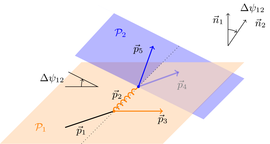
Figure 3: Azimuthal angles are defined between successive splitting planes for the $1\to 23$ splitting, $\mathcal{P}_{1}\supset\{\vec{p}_{2},\vec{p}_{3}\}$ and the $2\to 45$ splitting, $\mathcal{P}_{2}\supset\{\vec{p}_{4},\vec{p}_{5}\}$. The figure also depicts the vectors normal to the two planes, $\vec{n}_{1}$ and $\vec{n}_{2}$.

Each collinear branching in an event can be associated with the plane that contains the momenta of the two offspring partons. The simplest observable one may think of to study spin correlations is the azimuthal difference, $\Delta\psi$, between the planes defined by two distinct branchings. Here we will consider two broad cases: intra-jet correlations, i.e. between the planes of two branchings within a single jet, for example between the plane of the $1\to 56$ splitting and the plane of the $6\to 78$ splitting in Fig. 2; and inter-jet correlation, i.e. between the planes of two splittings in separate jets, for example between the plane of the $1\to 56$ splitting and the plane of the $2\to 34$ splitting in Fig. 2. We will refer to the two azimuthal differences as $\Delta\psi_{12}$ and $\Delta\psi_{11^{\prime}}$ where the $1$ and $2$ labels refer to the first and second splitting within a given jet and the $1^{\prime}$ label refers to the first splitting in a distinct jet. The $\Delta\psi_{12}$ and $\Delta\psi_{11^{\prime}}$ observables are straightforward to define at $\mathcal{O}\left(\alpha_{s}^{2}\right)$ relative to the hard scattering and it is this situation that we will concentrate on here. In the $\Delta\psi_{12}$ case, the splitting planes and the azimuthal angle between them are illustrated in Fig. 3.

At second order in the coupling, and in the collinear limit, the cross sections differential in the intra- and inter-jet observables $\Delta\psi_{12}$, respectively $\Delta\psi_{11^{\prime}}$, take the simple form (see e.g. section 2.3 in Ref [32], or the example calculated in Appendix B)

$$\frac{d\sigma}{d\Delta\psi_{ij}}\propto a_{0}\left(1+\frac{a_{2}}{a_{0}}\cos(2\Delta\psi_{ij})\right)=a_{0}\left(1+A_{i}(z_{i})B_{j}(z_{j})\cos(2\Delta\psi_{ij})\right)\,,$$ (11)

where the coefficients $a_{0}$ and $a_{2}$ depend on the observable, the final state under consideration, and the momentum fractions associated with the first ($z_{i}$) and second splitting ($z_{j}$). If the splittings are restricted to have opening angles greater than $e^{-|L|}$, with $|L|\gg 1$, and $\ln z_{1}$ and $\ln z_{2}$ are both of order $1$, the $a_{0}$ and $a_{2}$ coefficients are dominated by terms $\alpha_{s}^{2}L^{2}$, i.e. they belong to the single-logarithmic set of terms that we aim to control for NLL accuracy. For large $L$, at this order, the ratio $a_{2}/a_{0}$ is independent of $\alpha_{s}L$, and so Eq. (11) can always be written in terms of the functions $A(z)$ and $B(z)$ given in Table 2.

$\Delta\psi_{12}$
Primary splitting
$q\to qg$	$A(z)=\frac{2z}{1+z^{2}}$
$g\to gg$	$A(z)=\frac{z^{2}}{(1-z(1-z))^{2}}$
Secondary splitting
$g\to q^{\prime}\bar{q}^{\prime}$	$B(z)=\frac{-2z(1-z)}{1-2z(1-z)}$
$g\to gg$	$B(z)=\frac{z^{2}(1-z)^{2}}{(1-z(1-z))^{2}}$
$\Delta\psi_{11^{\prime}}$
$g\to q^{\prime}\bar{q}^{\prime}$	$A(z)=B(z)=\frac{-2z(1-z)}{1-2z(1-z)}$
$g\to gg$	$A(z)=B(z)=\frac{z^{2}(1-z)^{2}}{(1-z(1-z))^{2}}$

Table 2: The functions $A(z)$ and $B(z)$ entering Eq. (11) for the intra- and inter-jet observables $\Delta\psi_{12}$, $\Delta\psi_{11^{\prime}}$, for all channels at second order. See e.g. Appendix B for an exemplified derivation. Here, for a $1\to 23$ splitting, the variable $z$ is the momentum fraction carried away by parton $2$. Representative diagrams at $\mathcal{O}\left(\alpha_{s}^{2}\right)$ are shown on the right. In those diagrams, the splitting in black is the one associated with the corresponding function $A(z)$ or $B(z)$. The partons shown in grey serve as an example of what the rest of the branching history can look like, but they do not matter in choosing the function itself, since the contributions factorise in the final result, Eq. (11). Configurations that do not involve an intermediate gluon have vanishing spin correlations.

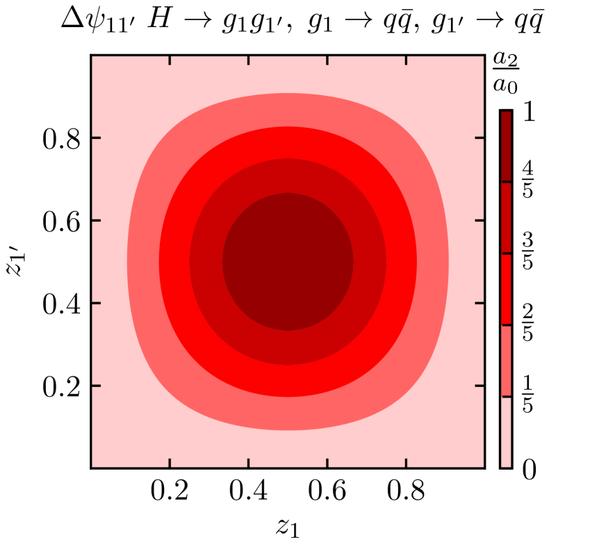
Figure 4: Size of the spin correlations, at fixed order $\mathcal{O}(\alpha_{s}^{2})$, for a quark-initiated jet. We consider the azimuthal difference $\Delta\psi_{12}$ between the splitting planes of a primary (with gluon momentum fraction $z_{1}$) and secondary ($z_{2}$) branching, separated by channel. The colour scale indicates the relative size $a_{2}/a_{0}$ of the correlations, where $\Delta\psi_{12}$ is distributed proportionally to $a_{0}+a_{2}\cdot{\rm cos}(2\Delta\psi_{12})$. Note the use of $z_{1}$ as the gluon momentum fraction in the $q\to qg$ splitting, while for amplitude expressions in the text, $z$ often refers to the quark momentum fraction.

In Fig. 4 we show a contour plot of the ratio $a_{2}/a_{0}=A(z_{1})B(z_{2})$, for our intra-jet observable, as a function of $z_{1}$ ($x$-axis) and $z_{2}$ ($y$-axis) for a quark-initiated jet. In this case there are only two non-trivial final states to consider, namely $q\rightarrow qg(g\rightarrow q^{\prime}\bar{q}^{\prime})$ and $q\rightarrow qg(g\rightarrow gg)$, while channels such as $q\to q(q\to qg)g$ that do not involve an intermediate gluon have vanishing spin correlations. In the case of $q\rightarrow qg(g\rightarrow q^{\prime}\bar{q}^{\prime})$, we see that the coefficient $a_{2}$ is negative, corresponding to an enhancement when the $q\to qg$ and $g\to q^{\prime}\bar{q}^{\prime}$ planes are perpendicular. The ratio $a_{2}/a_{0}$ peaks at $-100\%$ around $z_{1}=0$ and $z_{2}=0.5$, i.e. when the gluon is soft and the quark-antiquark pair share the energy equally. The spin correlations stay large even for moderate values of $z_{1}$ and $z_{2}$ although they vanish completely for $z_{1}\to 1$ (soft quark emerging from the $q\to qg$ splitting) and for $z_{2}\to 0$ or $z_{2}\to 1$ (either of the secondary $q^{\prime}$ or $\bar{q}^{\prime}$ becomes soft). Similarly, for $q\rightarrow qg(g\rightarrow gg)$, the ratio peaks at $z_{1}=0$ and $z_{2}=0.5$ but the correlation has the opposite sign to the $g\to q\bar{q}$ case, which implies an enhancement when the $q\to qg$ and $g\to gg$ splittings are in the same plane. The magnitude of $a_{2}/a_{0}$ is substantially smaller, with a peak at $1/9$. The spin correlations fall off more sharply than in the $g\rightarrow q^{\prime}\bar{q}^{\prime}$ case, in particular as a function of $z_{2}$, and also vanish for $z_{1}\to 1$ and for $z_{2}\to 0$ or $z_{2}\to 1$.

The overall picture is very similar for a gluon-initiated jet, shown in Fig. 5, although the dependence on $z_{1}$ is moderately stronger for both $g\to q^{\prime}\bar{q}^{\prime}$ and $g\to gg$ secondary splittings, which can be understood from Table 2.

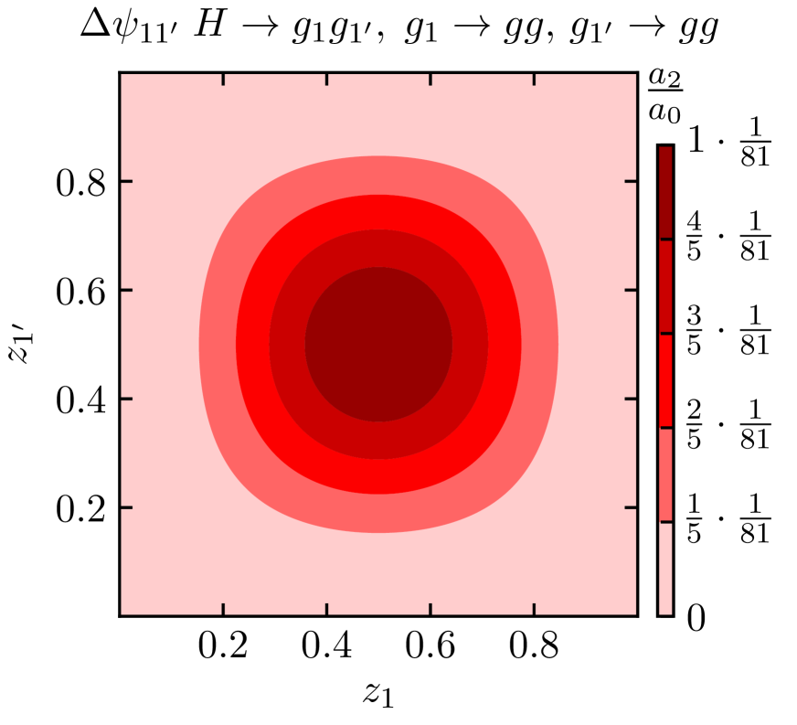
Figure 5: Same as Fig. 4, for a gluon-initiated jet. Note that the colour scale is spanning the same range as in Fig. 4.

Turning now to the correlations between azimuthal angles in two distinct jets, they are zero for a $\gamma^{*}\to q\bar{q}$, but non-zero for $H\to g_{1}g_{1^{\prime}}$, so we consider only the latter. In this case we examine the azimuthal difference $\Delta\psi_{11^{\prime}}$ between the splitting planes of the two primary emissions. There are three possible final states given by $\{g_{1}\rightarrow q\bar{q},g_{1^{\prime}}\rightarrow q\bar{q}\}$, $\{g_{1}\rightarrow q\bar{q},g_{1^{\prime}}\rightarrow gg\}$, and $\{g_{1}\rightarrow gg,g_{1^{\prime}}\rightarrow gg\}$.

Figure 6: Same as Figs. 4 and 5, for a $H\to gg$ event, where we consider the azimuthal difference $\Delta\psi_{11^{\prime}}$ between the splitting planes of the two primary branchings on each side of the event. Note the different scale of the colour bar for the inter-jet observable: here, the spin correlations are largest for the quark-only final-state (top left) which peak at $+100\%$, mid-range for the mixed quark-gluon final state (top right) peaking at $-11.1\%$, and much smaller for the all-gluon final state (bottom), with a peak at $+1.23\%$.

In Fig. 6 we show the ratio $a_{2}/a_{0}$ as a function of the energy fractions $z_{1}$ and $z_{1^{\prime}}$. In all three cases the ratio is peaked when $z_{1}=z_{1^{\prime}}=0.5$ and is largest in magnitude when both gluons split into quark-antiquark pairs. When only one gluon splits into a quark-antiquark pair the ratio becomes negative and $-11.1\%$ around the peak. When both gluons split into gluons the spin correlations almost vanish. In all three cases the ratio vanishes when either of the energy fractions approach $0$ or $1$.

3.2 Definition of spin-sensitive Lund observables

The observables discussed so far start at $\mathcal{O}(\alpha_{s}^{2})$ relative to the hard scattering, but care has to be taken in order to define them in an infrared safe way beyond that order. To facilitate a definition which can also be directly applied in experimental analyses, we make use of the procedure from Ref. [44] to build Lund diagrams [26] from individual jets. We remind the reader that the Lund jet plane is constructed through a declustering of a C/A-jet [45, 46]. The primary Lund plane is constructed by following the harder branch at each step of the declustering. If at some point one instead follows a softer branch and then all its subsequent harder branches, those subsequent branches populate a secondary Lund plane.

The procedure that we describe here can be applied at hadron colliders and $e^{+}e^{-}$ colliders (or also in the decay of heavy particles at hadron colliders, for example in their rest frame). The first branching within a jet is identified by taking all declusterings on the primary Lund plane that satisfy $z$ larger than some $z_{\text{cut}}$, and selecting the one with largest relative $k_{t}$. The second branching within a jet is identified by taking all declusterings on the secondary Lund plane associated with the first branching, and then again identifying those that satisfy $z$ larger than some $z_{\text{cut}}$ and selecting the one with largest relative $k_{t}$. One may choose to use different $z_{\text{cut}}$ values for the first and second branchings within a single jet. Given a choice of $z_{\text{cut}}$, one may then study the results differentially in the two $z$ values, so as to obtain plots similar to Figs. 4–6. Here, however, we will consider just results integrated over $z$. Note that in section 3.1, we investigated the structure for $0<z<1$, while in the Lund construction we always have $z\leq 1/2$, because $z$ is the momentum carried by the softer offspring (and the secondary Lund plane is the one associated with further emission from the softer offspring). So, for example, in section 3.1 we could meaningfully discuss a $q\to qg$ splitting where the quark was soft ($z_{1}$ close to $1$), followed by a splitting of the gluon. In contrast, in the Lund declustering picture, the quark in such a case will be assigned to the secondary plane, and the second splitting that we study will necessarily be a further $q\to qg$ splitting. The reason for adopting this procedure in Lund declustering is that experimentally one cannot observe the flavour of the underlying parton.

To track the azimuthal angles in the $e^{+}e^{-}$ case within the Lund declustering, we adopt a procedure that differs from that introduced in Ref. [24] (supplemental material), because we have found that the latter results in differences in azimuthal angles that are not invariant under rotations of the event. We start with an initial azimuthal angle $\psi_{0}=0$ (the particular choice has no impact on the differences of azimuthal angles that we eventually study). Then, working through the declusterings in the Cambridge/Aachen sequence, for each declustering $i$ we:

1. Compute the normalised cross product, $\hat{n}_{i}=\vec{p}_{i,a}\times\vec{p}_{i,b}/|\vec{p}_{i,a}\times\vec{p}_{i,b}|$, between the two pseudojets, $\vec{p}_{i,a}$ and $\vec{p}_{i,b}$ that result from the declustering, where $\vec{p}_{i,a}$ is the harder of the two.

2. Compute the signed angle $\Delta\psi_{(i-1,i)}$ between $\hat{n}_{i-1}$ and $\hat{n}_{i}$ where $\Delta\psi_{(i-1,i)}$ is positive if $\left(\hat{n}_{i-1}\times\hat{n}_{i}\right)\cdot\vec{p}_{i,a}>0$ and negative otherwise, and ${\hat{n}}_{i-1}$ is the normalised cross product obtained for the splitting that produced the parent parton.

3. Compute $\psi_{i}=\psi_{i-1}+\Delta\psi_{(i-1,i)}$.

The variable $\Delta\psi_{12}$ is now defined as the difference between the $\psi$ obtained for the primary splitting and secondary splittings as selected above (which may not follow in immediate sequence in the C/A declustering). For the case of two successive splittings, this is equivalent to the $\Delta\psi_{12}$ illustrated in Fig. 3. Likewise we define $\Delta\psi_{11^{\prime}}$ as the $\psi$ difference between the highest-$k_{t}$ primary passing the $z>z_{\text{cut}}$ requirement inside each of the two different jets. The Lund diagrams are illustrated at second order in Figs. 7 and 8.

In practice, in our $e^{+}e^{-}$ implementation of the $\Delta\psi_{12}$ observable, we cluster the event back to two jets and analyse each jet independently. Our final distributions will be normalised to the number of events, rather than the number of jets.

Figure 7: For the intra-jet definition of the Lund observable $\Delta\psi_{12}$, we consider the primary $q\to qg_{1}$ and secondary splittings $g_{1}\to g_{1}g_{2}$ (left) and $g_{1}\to q^{\prime}\bar{q}^{\prime}$ (right). We apply a cut (dashed lines), $z_{\rm cut}$, on the momentum fraction used to identify the primary and secondary splittings. The red (blue) dots indicate that the azimuthal angles in those splittings are correlated, with the preferred value of $\Delta\psi_{12}$ being in-plane (out-of-plane).

Figure 8: For the inter-jet definition of the Lund observable $\Delta\psi_{11^{\prime}}$, to be used in $H\to gg$ events, we consider two primary splittings in different hemispheres.

3.3 Recall of 3-point energy-correlator observable

Recently Chen, Moult and Zhu proposed 3-point energy correlators (EEEC) as suitable observables for measuring the quantum interference effects associated with spin correlations [38]. For concreteness, we use the following definition for the EEEC,

$$\frac{1}{\sigma_{\text{tot}}}\frac{d^{3}\Sigma}{d\Delta\psi d\theta_{S}d\theta_{L}}=\left\langle\sum_{i,j,k=1}^{N}\frac{8E_{i}E_{j}E_{k}}{Q^{3}}\delta\left(\Delta\psi-\phi_{(ij)k})\right)\delta\left(\theta_{S}-\theta_{ij}\right)\delta\left(\theta_{L}-\theta_{jk}\right)\right\rangle$$ (12)

where $\sigma_{\text{tot}}$ is the total cross section, $Q$ is the event centre-of-mass energy, $\theta_{mn}$ is the opening angle between two emissions $m$ and $n$ and $\phi_{(ij)k}$ is the angle between the plane that contains the $p_{i}+p_{j}$ and $p_{k}$ directions and the plane that contains the $p_{i}$ and $p_{j}$ directions. The average is carried out across events, and in each event the sum over each of the $i$, $j$ and $k$ runs over all particles in the event, $1\ldots N$. One may also apply the definition to particles in a single jet of energy $E_{\text{jet}}$, in which case one would replace $8/Q^{3}$ with $1/E_{\text{jet}}^{3}$. Refs. [58, 38] provided techniques for resumming such observables, and below we will compare our resummation results for the EEEC to theirs.

3.4 MicroJets resummation of spin correlations and comparison to fixed order

Although the above fixed-order analysis gives a sense of the overall structure of spin correlations in quark- and gluon-initiated jets, there are important effects which can only be captured by all-order resummation.

To our knowledge, no analytical result exists for the logarithmic structure of observables sensitive to spin correlations, except for the recently computed all-order result [38] for the 3-point energy correlator, reproduced in section 3.3. In order to enable comparisons to other observables we have implemented a numerical resummation, henceforth called the toy shower, based on the MicroJets code [39, 40, 59].

The toy shower is ordered in an angular-type evolution variable $t$,

$$t(\theta,p_{t})=\int_{\theta}^{1}\frac{d{\theta^{\prime}}}{\theta^{\prime}}\frac{\alpha_{s}(E\theta^{\prime})}{\pi}\;,$$ (13)

where $E$ is the energy of the hard parton initiating the shower, and $\theta$ is an angular scale. For a 1-loop running of the strong coupling $\alpha_{s}(p_{t}\theta)$, the scale $t$ is related to the opening angle of the splitting $\theta$ by

$$t=\frac{1}{\beta_{0}}\ln\left(\frac{1}{1+\frac{\alpha_{s}}{\pi}\beta_{0}\ln\theta}\right)=\frac{1}{\beta_{0}}\ln\left(\frac{1}{1+\frac{\lambda}{\pi}\beta_{0}}\right)\,,$$ (14)

where $\beta_{0}=\frac{1}{6}(11C_{A}-4T_{R}n_{f})$, and where we have introduced $\lambda=\alpha_{s}\ln\theta$. Single-logarithmic terms of the form $(\alpha_{s}{\ln}(1/\theta))^{n}$ can then be resummed by solving corresponding DGLAP-style equations. Unlike in a real parton shower, there is no kinematic map associated with the emissions, and crucially it thus does not generate any spurious higher-order terms. Since the toy shower is angular ordered, the Collins-Knowles algorithm can readily be applied to it, and we can make predictions for angular observables correct at NLL in the strongly ordered limit. The toy shower can also provide fixed order predictions at $\mathcal{O}(\alpha_{s}^{2})$ in the collinear limit.

3.4.1 Results for Lund declustering observables

We start by evaluating the impact of the single-logarithmic resummation on the size of the spin correlations, $a_{2}/a_{0}$, for the observables $\Delta\psi_{12}$ and $\Delta\psi_{11^{\prime}}$ introduced above. In order to do so, we consider the distributions of $\Delta\psi_{12}$ and $\Delta\psi_{11^{\prime}}$ generated by the toy shower for a value of $t_{\rm max}=\frac{0.5}{\pi}$, which corresponds to $\lambda\approx-0.3743$ for a 1-loop running of the strong coupling, see Eq. (14), which is compatible with the range of $\alpha_{s}$ and $L$ accessible at the LHC (cf. table 1 of Ref. [25]). We then apply the Lund declustering procedure: we identify a splitting as primary or secondary only if it passes the cut $z>z_{\rm cut}$. We then determine the coefficients $a_{0}$ and $a_{2}$ from the distribution of the observable.

(a) $q\rightarrow qg(g\rightarrow gg)$

(b) $q\rightarrow qg(g\rightarrow q^{\prime}\bar{q}^{\prime})$

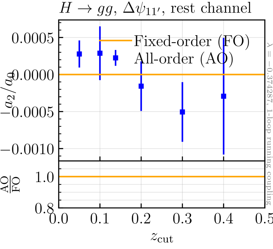
(c) All channels

Figure 9: Relative size of the spin correlations $a_{2}/a_{0}$ for $\Delta\psi_{12}$, in $\gamma^{*}\to q\bar{q}$ (quark-initiated jet), from a numerical resummation (AO, blue triangles), compared to the second-order result (FO, orange curve) for (a) the $gg$, (b) the $q^{\prime}\bar{q}^{\prime}$ and (c) all channels.

(a) $q\rightarrow qg(g\rightarrow gg)$

(b) $q\rightarrow qg(g\rightarrow q^{\prime}\bar{q}^{\prime})$

(c) All channels

Figure 10: Same as Fig. 9, for $H\to gg$ (gluon-initiated jet).

Figure 9 depicts the ratio $a_{2}/a_{0}$ at fixed second order (FO) and all orders (AO) for the case of $\Delta\psi_{12}$ in $\gamma^{*}\to q\bar{q}$ events (quark-initiated intra-jet azimuthal angle), for five values of $z_{\rm cut}\in\{0.05,0.1,0.2,0.3,0.4\}$ (the fixed order extends to $z_{\text{cut}}=0$, however the resummation cannot be extended to that region without also addressing soft logarithms). The size of the spin correlations is shown separately for the two different branching histories $q\rightarrow qg(g\rightarrow gg)$ in Fig. 9(a), and $q\rightarrow qg(g\rightarrow q^{\prime}\bar{q}^{\prime})$ in Fig. 9(b). The rest channel, characterised by the absence of an intermediate gluon (e.g. $q\rightarrow gq(q\rightarrow gq)$ at second order, and other possible histories at all orders), is not shown as it does not produce correlations. The ratio $a_{2}/a_{0}$ is also given for the sum of all channels in Fig. 9(c).

Turning on the IR cut, $z_{\rm cut}>0$, first leads to an increase in the absolute size of $|a_{2}/a_{0}|$, with the large-$z_{2}$ contributions in Fig. 4 driving the spin correlations. As $z_{\rm cut}$ continues to increase, the intermediate gluon becomes harder and spin correlations decrease again up to $z_{\rm cut}=0.5$. We observe that the size of the spin correlations agrees between the fixed order and the resummed, all-order case, for small values of $z_{\rm cut}\sim 0$, in the separate channels. Once we turn $z_{\rm cut}$ on, the resummation starts diluting the spin correlations, as intermediate, soft gluons can be emitted with values of $z<z_{\rm cut}$, transporting away some of the spin information before it is propagated to the identified secondary splitting. Thus, the size of the correlations in the resummed prediction decreases with respect to the fixed-order calculation, with the resummed $|a_{2}/a_{0}|$ being about $88\%$ of the fixed-order value at $z_{\rm cut}=0.4$.

If one considers the sum of all channels, given in Fig. 9(c), i.e. without the inclusion of any flavour-tagging, the relative size of the resummed correlations starts at about $95\%$ of their fixed-order counterpart at small values of $z_{\rm cut}\sim 0$. This decrease finds its source in the higher relative contribution from possible branching histories without correlations — what we call the rest channel — in all-order events: indeed, there is only one such possible history at second order ($q\to q(q\to qg)g)$, where the emission of the first gluon is hard and the declustering follows the soft quark branch to the secondary splitting). This rest channel contributes to $a_{0}$ but not to $a_{2}$, thus the additional damping of $|a_{2}/a_{0}|$ at small values of $z_{\rm cut}$ in

$$\left(\frac{a_{2}}{a_{0}}\right)_{\text{\!all}}=\frac{a_{2,{\rm q^{\prime}\bar{q}^{\prime}}}+a_{2,{\rm gg}}}{a_{0,{\rm q^{\prime}\bar{q}^{\prime}}}+a_{0,{\rm gg}}+a_{0,{\rm rest}}}\,.$$ (15)

Similar results are shown in Fig. 10 for the gluon-initiated ($H\to gg$) intra-jet observable $\Delta\psi_{12}$. While the spin correlations are smaller when compared to the quark-initiated case presented above, we find that they are also less sensitive to resummation: the all-order correlations $|a_{2}/a_{0}|$ are about $\mathcal{O}(95\%)$ of their fixed-order counterpart at $z_{\rm cut}=0.4$ for the separate channels, and $\mathcal{O}(92.5\%)$ for the sum of all channels.

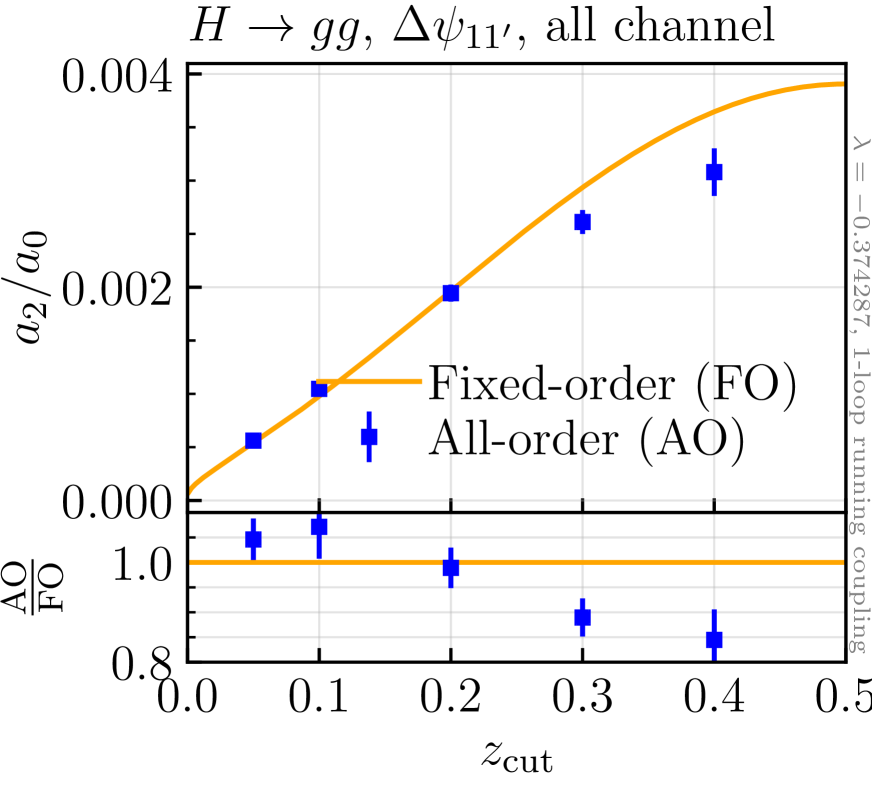
(a) $\{g_{1}\rightarrow gg,g_{1^{\prime}}\rightarrow gg\}$

(b) $\{g_{1}\rightarrow q\bar{q},g_{1^{\prime}}\rightarrow gg\}$

(c) $\{g_{1}\rightarrow q\bar{q},g_{1^{\prime}}\rightarrow q\bar{q}\}$

(d) All channels

Figure 11: Size of the correlations $a_{2}/a_{0}$ in $\Delta\psi_{11^{\prime}}$ for $H\to gg$ events (inter-jet). Results are shown for (a) the $gggg$, (b) the $ggq\bar{q}$ , (c) the $q\bar{q}q\bar{q}$ and (d) all channels.

Finally, fixed- and all-order predictions are shown in Fig. 11 for the inter-jet observable $\Delta\psi_{11^{\prime}}$ in $H\to g_{1}g_{1^{\prime}}$ events. The correlations $|a_{2}/a_{0}|$ are very small in each separate channel, with the exception of the all-quark final state $g_{1}\to q\bar{q},g_{1^{\prime}}\to q^{\prime}\bar{q}^{\prime}$. Because the largest cross section comes from the all-gluon final state, where the correlations $|a_{2}/a_{0}|\lesssim 1\%$ are extremely small, and because of partial cancellations between different channels, the correlations in the sum of all channels are almost vanishing. Since the effect is so small, there is a large statistical uncertainty on the value of the coefficient $a_{2}$ fitted from the Monte-Carlo runs of the toy shower. It still gives results consistent with the observations made above. Additionally, we note that the inter-jet spin correlations are also somewhat more sensitive to resummation than for the intra-jet correlations in $\Delta\psi_{12}$ studied above.

3.4.2 Validation and results for energy correlators

As part of the validation of the MicroJets code, we also compare it to the analytic resummation of the EEEC presented in Ref. [38]. While in the latter reference, the spin correlations in the EEEC were shown differentially as a function of the opening angle $\theta_{S}$ of the secondary (small) splitting and fixed opening angle $\theta_{L}$ of the primary (large) splitting, here we show the results integrated over angles to enhance the statistics. Inspired by Ref. [38] we choose the following integration bounds on the opening angles of the primary and secondary branchings:

$$\sqrt{0.1} <\theta_{L}<1\,,$$

$$0.01 <\theta_{S}<0.1\,,$$ (16)

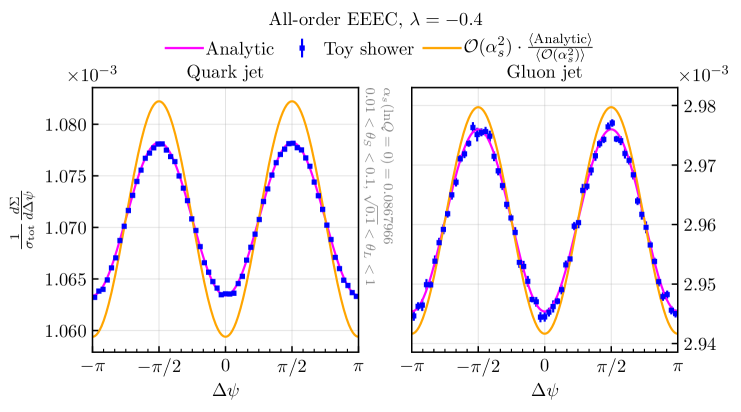
Figure 12: All-order comparison of the toy shower and the analytic resummation performed in Ref. [38], for a quark-initiated (left) and a gluon-initiated jet (right). The resummation is performed using $\alpha_{s}=0.0868$ and restricting the opening angles as in Eq. (16). The result from a fixed-order expansion, normalised so that its mean coincides with the mean value of the analytic curve, is also shown for comparison.

and take $\alpha_{s}=0.0868$ corresponding to a hard scale of roughly $1~{}\mathrm{TeV}$. The toy shower and analytic resummation results [38] are shown in Fig. 12, summed over all final branching flavour channels, demonstrating good agreement. The figure also shows the second-order expansion, normalised so that its mean value coincides with the resummed result, illustrating a modest reduction in the degree of spin correlations from the resummation, which is similar to our findings above with the Lund declustering observables.

4 Numerical validation of spin correlations within PanScales showers

In this section, we validate the PanScales showers against various numerical predictions. In particular we want to demonstrate that the algorithm described above reproduces fixed-order matrix elements in the strongly ordered limit and that it produces the correct NLL distributions at all orders. Here, we first provide a brief summary of the PanScales showers. A comprehensive description can be found in Ref. [24].

The PanScales showers fit into two categories, namely PanLocal which features local recoil, and PanGlobal which features global recoil. The PanLocal mapping for the emission of $p_{k}$ from a dipole $\{\tilde{p}_{i},\tilde{p}_{j}\}$ is given by

$$p_{k} =a_{k}\tilde{p}_{i}+b_{k}\tilde{p}_{j}+k_{\perp}\,,$$ (17a)

$$p_{i} =a_{i}\tilde{p}_{i}+b_{i}\tilde{p}_{j}-fk_{\perp}\,,$$ (17b)

$$p_{j} =a_{j}\tilde{p}_{j}+b_{j}\tilde{p}_{j}-(1-f)k_{\perp}\,,$$ (17c)

where $k_{\perp}=k_{\perp,1}\cos(\varphi)+k_{\perp,2}\sin(\varphi)$ and $-k_{\perp}^{2}=k_{t}^{2}$. The coefficients of the map are functions of the ordering variable, $v$, and an auxiliary variable $\bar{\eta}$,

$$v=\frac{k_{t}}{\rho}e^{-\beta|\bar{\eta}|},\qquad\rho=\left(\frac{s_{{\tilde{\imath}}}s_{{\tilde{\jmath}}}}{Q^{2}s_{{\tilde{\imath}}{\tilde{\jmath}}}}\right)^{\frac{\beta}{2}}\,,\qquad a_{k}=\sqrt{\frac{s_{{\tilde{\jmath}}}}{s_{{\tilde{\imath}}{\tilde{\jmath}}}s_{{\tilde{\imath}}}}}\,k_{t}{e}^{+\bar{\eta}}\,,\qquad b_{k}=\sqrt{\frac{s_{{\tilde{\imath}}}}{s_{{\tilde{\imath}}{\tilde{\jmath}}}s_{{\tilde{\jmath}}}}}\,k_{t}{e}^{-\bar{\eta}}\,,$$ (18)

where $s_{{\tilde{\imath}}{\tilde{\jmath}}}=2{\widetilde{p}}_{i}\cdot{\widetilde{p}}_{j}$, $s_{{\tilde{\imath}}}=2{\widetilde{p}}_{i}\cdot Q$, and $Q$ is the total event momentum. The quantity $\beta$ parameterises the choice of ordering variable. The PanGlobal map drops the $k_{\perp}$-contributions to $p_{i}$ and $p_{j}$, as well as the terms $b_{i}$ and $a_{j}$, and instead boosts and rescales the full event. The PanLocal shower comes in a dipole variant, where $f=1$ and every soft eikonal is reproduced by the sum of two opposite branching kernels, and in an antenna variant, where

$$f=f(\bar{\eta})=\frac{e^{2\bar{\eta}}}{1+e^{2\bar{\eta}}}\,,$$ (19)

and every eikonal is instead contained in a single contribution. We will show results for the PanGlobal shower with $\beta=0$ and the PanLocal dipole shower with $\beta=1/2$ and in some places also the PanLocal antenna shower with $\beta=1/2$.

4.1 Validation at second order

The first essential test to carry out is at fixed $\mathcal{O}(\alpha_{s}^{2})$ since this is the first order at which spin correlations are non-vanishing. We compare the collinear branching amplitudes presented in section 2.1 against the exact $\mathcal{O}(\alpha_{s}^{2})$ tree-level matrix element, taking the limit of strongly ordered angles for fixed $z_{1}$ and $z_{2}$. We then proceed to validate our adaptation of the Collins-Knowles algorithm by applying it at fixed order in the PanScales showers and comparing against the second order expansion of the toy shower and the exact $\mathcal{O}(\alpha_{s}^{2})$ cross section.

4.1.1 Matrix element validation of collinear branching amplitudes

Matrix elements constructed using collinear branching amplitudes are expected to reproduce the exact amplitudes only in the strongly ordered limit. In order to demonstrate that this is the case, we consider the angular correlations $\Delta\psi_{12}$ and $\Delta\psi_{11^{\prime}}$ as a function of

$$\Theta_{12} =\max\left(\theta_{1},\theta_{2}/\theta_{1}\right),$$

$$\Theta_{11^{\prime}} =\max\left(\theta_{1},\theta_{1^{\prime}}\right),$$ (20)

where $\theta_{i}$ is the opening angle of the $i^{\text{th}}$ branching. The strongly ordered limit is then approached as $\Theta\rightarrow 0$. In practice we achieve this by fixing the energy fractions $z_{1}$ and $z_{2}$. We then generate angles $\theta_{1}$, $\theta_{2}$, $\phi_{1}$, and $\phi_{2}$ from which we can deduce the full kinematics of our event using the PanLocal dipole $\beta=0.5$ map. The full kinematics are then passed to the exact matrix element, obtained using amplitudes from Ref. [60], to be compared directly with the Collins-Knowles weights, Eqs. (1) and (2).

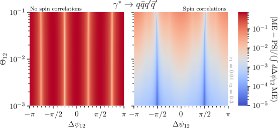
Figure 13: Normalised difference between the Collins-Knowles weight and the full squared matrix element for $e^{+}e^{-}\to\gamma^{*}\to q\bar{q}+\text{2-parton}$ events. Both branchings are on the same side of the event and have $z_{1}=0.01$ and $z_{2}=0.3$. The left-hand (right-hand) column shows the results when we neglect (include) spin-correlations in the Collins-Knowles weights. The rows show different partonic channels.

In Fig. 13 we show this comparison as a function of $\Delta\psi_{12}$ and $\Theta_{12}$ for the processes $\gamma^{*}\rightarrow q\bar{q}q^{\prime}\bar{q}^{\prime}$ and $\gamma^{*}\rightarrow q\bar{q}gg$ for $z_{1}=0.01$ and $z_{2}=0.3$. On the left we show the comparison between the exact matrix element and the shower matrix element without spin correlations, while they are included on the right. We show the absolute difference between the exact matrix element and the shower matrix element normalised to the exact matrix element integrated in a slice of $\Delta\psi_{12}$. When spin correlations are not included in the branching amplitudes the exact matrix element and the shower matrix element disagree for all values of $\Theta_{12}$ and $\Delta\psi_{12}$ in both processes. The band structure that shows up for $\Delta\psi_{12}=\{\frac{-3\pi}{4},\frac{-\pi}{4},\frac{\pi}{4},\frac{3\pi}{4}\}$ corresponds to the points in $\Delta\psi_{12}$ where the azimuthal modulation of the full matrix element intersects the prediction by the shower, which is flat in the collinear limit. When spin correlations are included we see that the discrepancy between the exact matrix element and the shower matrix element only persists away from the collinear limit and we find that the residual differences vanish as $\Theta_{12}$ becomes small.

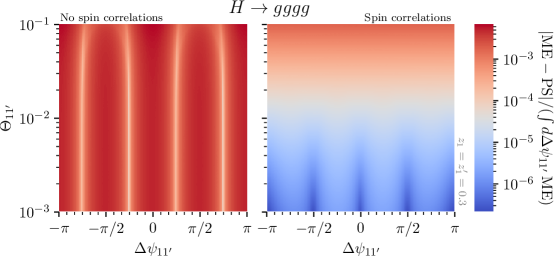
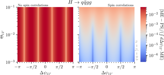
Figure 14: Same as Fig. 13 but for $H\to gg+\text{2-parton}$ events. The two branchings are on opposite sides of the event and have $z_{1}=z_{1^{\prime}}=0.3$.

The picture is very similar if we instead focus on $H\rightarrow gg$ processes, as can be seen in Fig. 14. In this case we show the three subprocesses $H\rightarrow gggg$, $H\rightarrow ggq\bar{q}$, and $H\rightarrow q\bar{q}q^{\prime}\bar{q}^{\prime}$ as a function of $\Delta\psi_{11^{\prime}}$ and $\Theta_{11^{\prime}}$, using $z_{1}=z_{2}=0.3$. When spin correlations are not included in the shower branching amplitudes, the shower matrix element and the exact matrix element again disagree for all values of $\Theta_{11^{\prime}}$ and $\Delta\psi_{11^{\prime}}$. The same band structure can be seen as in Fig. 13 which is again due to the intersection of the cosine and an almost flat curve. When spin correlations are included in the shower we again find excellent agreement as we approach the strongly ordered limit. Some band structure remains, associated with the existence of azimuths for which the exact and parton shower results happen to coincide exactly.

4.1.2 Tests with full shower phase space and observables

We now consider integrated results over a portion of the Lund plane, i.e. using the analysis approach discussed in section 3.2. This serves to test the full combination of shower phase space generation, branching probabilities and observable implementation (which comes in independent variants for the toy shower and the full shower). We still work at fixed (second) order, and compare the resulting distribution of $\Delta\psi_{12}$ for several of the PanScales showers, the toy shower, and the exact tree-level matrix element. We produce results for a fixed strong coupling at $Q=100\,{\rm TeV}$, setting the following cuts on the primary and secondary splittings:

$$z_{1}>0.1,\quad k_{t,1}<1\,{\rm TeV}\,,$$ (21a)

$$z_{2}>0.2,\quad k_{t,2}>1\,{\rm GeV}\,.$$ (21b)

Fig. 15 depicts the second-order (normalised) differential cross-section

$$\frac{1}{\sigma_{\text{tot}}}\frac{d\sigma}{d\Delta\psi_{12}}=\frac{1}{\int d|{\rm ME}_{\gamma^{*}\to q\bar{q}}|^{2}}\frac{d|{\rm ME}_{\gamma^{*}\to q\bar{q}+X}|^{2}}{d\Delta\psi_{12}}\,,$$ (22)

for different values of $\Theta_{12}$, where $X$ may be $q\bar{q}$ or $gg$. As in the previous section, the latter variable serves as a measure of ordered collinearity for the two successive splittings. We show the distributions obtained by the toy shower, by the PanLocal shower (run with a value of $\beta=0.5$, see Eq. (18)) in its dipole formulation, and by the exact tree-level matrix element. In the bulk of the phase space, where opening angles are not strongly restricted, the distribution of $\Delta\psi_{12}$ is not expected to agree across all considered setups: the parton shower will feature non-negligible recoil effects, and the toy shower is applying the strictly-collinear limit of the Collins algorithm irrespective of the opening angles. However, we do expect agreement between those setups, and the exact matrix element, in the limit where the angles are small and strongly ordered.

To quantify the agreement between the different setups in the strongly-ordered collinear limit, ${\rm lim}_{\Theta_{12}\to 0}\left(\frac{d\sigma}{d\Delta\psi_{12}}\right)$, we apply a Discrete Cosine Transform (DCT) to the binned distribution of $\Delta\psi_{12}$, where we integrate over all configurations that fulfil the strong angular ordering requirement for a given value of $\Theta_{12}$. Specifically, for a distribution with $\Delta\psi_{12}$ bins running from $i=0,\ldots,n-1$ we define the $k^{\text{th}}$ DCT coefficient as follows

$$A_{k}(\Theta_{12})=\frac{1}{n}\sum_{i=0}^{n-1}\cos\left(\frac{2k\pi}{n}\left(i+\frac{1}{2}\right)\right)\int_{\text{bin }i}\!\!\!\!d\Delta\psi_{12}\int_{\begin{subarray}{c}\theta_{1}<\Theta_{12}\hphantom{\theta_{1}}\\ \theta_{2}<\Theta_{12}\theta_{1}\end{subarray}}d\theta_{2}d\theta_{1}\frac{d\sigma}{d\theta_{1}d\theta_{2}d\Delta\psi_{12}}\,.$$ (23)

The $A_{0}$ and $A_{2}$ coefficients can be related to the Fourier coefficients $a_{0}$ and $a_{2}$ used above,

$$a_{0}=A_{0}\,,\qquad a_{2}=2A_{2}\,.$$ (24)

This definition exclusively picks out the even (cosine-like) Fourier components, whereas the odd (sine-like) modes are zero by definition.

The results are summarised in Fig. 16, for $\gamma^{*}\to q\bar{q}q^{\prime}\bar{q}^{\prime}$ (left column) and $\gamma^{*}\to q\bar{q}gg$ (right column). We show the first four DCT coefficients, normalised by the toy shower $A_{0}^{ts}(\Theta_{12})$, for two PanScales showers, the exact matrix element, and the toy shower. For the latter, since the toy shower is free of recoil effects, the correlations introduced by the spin algorithm take the form given by Eq. (11) irrespective of the value of $\Theta_{12}$. Thus, for the toy shower, $A_{0}$ and $A_{2}$ are the only non-zero coefficients, and $2A_{2}/A_{0}=a_{2}/a_{0}$ gives the relative size of the integrated spin correlations, which are of the order $\mathcal{O}(-77\%)$ for the $g\to q^{\prime}\bar{q}^{\prime}$ channel, and $\mathcal{O}(+7\%)$ for the $g\to gg$ channel in most of the phase space. The parton showers and the matrix element partly generate non-zero coefficients at large values of $\Theta_{12}$, all of which become consistent with zero in the strongly-ordered limit at $\ln\Theta_{12}\sim-4$, with the exception of the coefficient $A_{2}$ encoding the spin correlations. All setups produce compatible values of $A_{2}$ at small $\Theta_{12}$. We also observe that the PanScales showers display distortions that are of same sign, and similar in size, as the exact matrix element at larger values of $\Theta_{12}$. The difference between the PanLocal dipole and the PanGlobal showers is a consequence of the different kinematic map rather than the difference in $\beta$ values that we have used ($0.5$ and $0.0$ respectively).

(a) $q\bar{q}q^{\prime}\bar{q}^{\prime}$

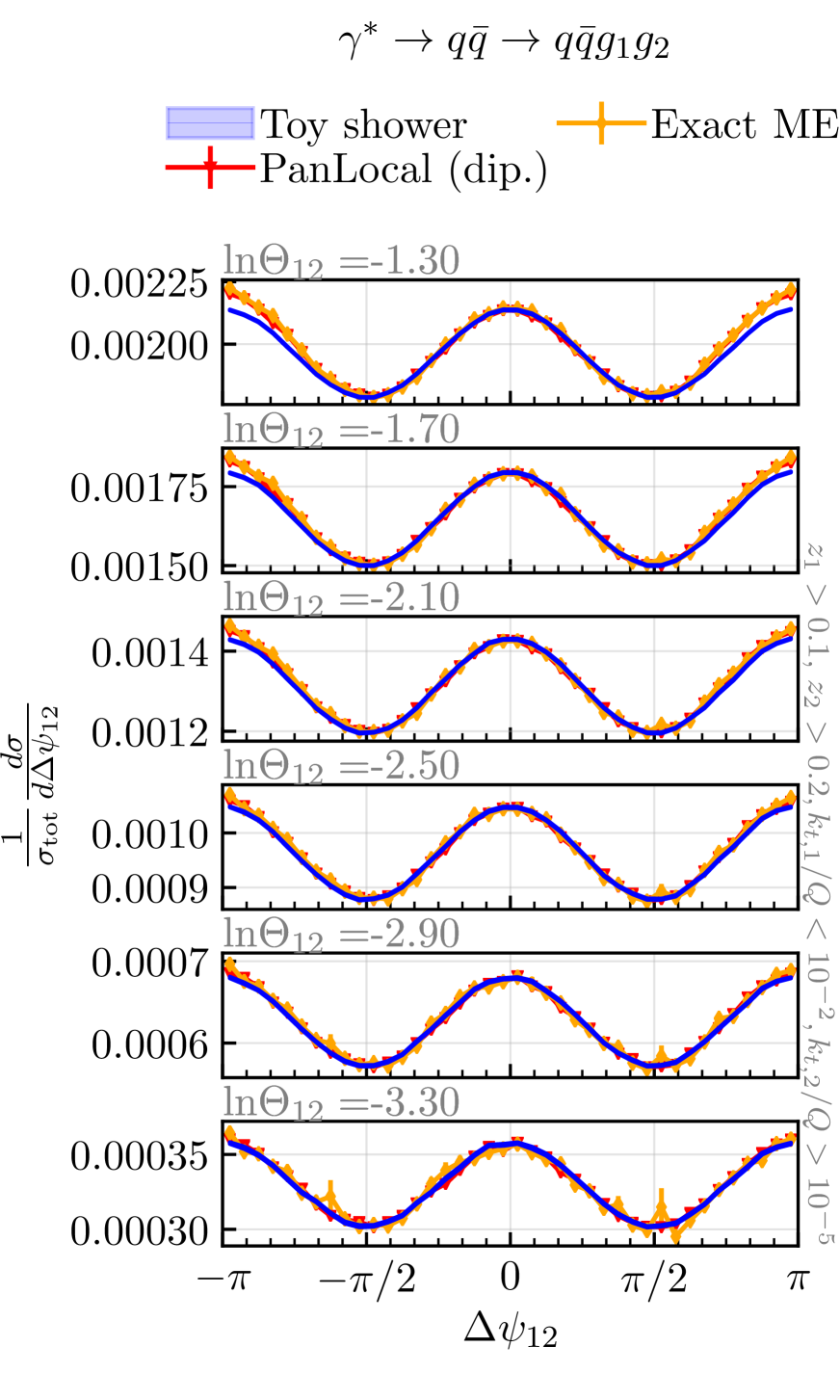
(b) $q\bar{q}g_{1}g_{2}$

Figure 15: The second-order distribution of $\Delta\psi_{12}$ from the toy shower, the dipole PanLocal shower, and the tree-level matrix element, shown for increasingly collinear configurations, ${\ln}\Theta_{12}\in\{-1.3,-1.7,-2.1,-2.5,-2.9,-3.3\}$. Results are given for (a) quark-only and (b) two quarks-two gluons final states.

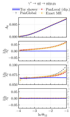
Figure 16: Fixed-order Fourier analysis of the toy shower, the PanGlobal $(\beta=0)$, and the dipole PanLocal ($\beta=0.5$) showers, as compared to the exact tree-level matrix element. The first four modes are shown here, and their associated coefficients suitably converge to identical values in the strongly angular-ordered limit $\Theta_{12}\to 0$.

4.2 Validation at all orders in $\alpha_{s}$

We now turn to the validation of our spin-correlation algorithm in the PanScales parton showers. To test specifically the single logarithmic (NLL), $\alpha_{s}^{n}L^{n}$, terms generated by the shower, we run the PanGlobal ($\beta=0$) shower and the dipole and antenna versions of the PanLocal ($\beta=0.5$) showers with asymptotically small $\alpha_{s}\to 0$, keeping $\lambda=\alpha_{s}L$ fixed. For the Lund declustering observable (cf. section 3.2), $e^{-|L|}$ is the smallest value that we allow for $k_{t,2}/Q$, or equivalently at $\alpha_{s}^{n}L^{n}$ accuracy, the smallest value for $\theta_{2}$, while $\theta_{1}$ and $k_{t,1}$ are allowed to take on any value (typically, the Lund declustering procedure ensures $\theta_{1}>\theta_{2}$ and $k_{t,1}>k_{t,2}$). For the EEEC variable (cf. section 3.3), $e^{-|L|}$ is the smallest value that we allow for $\theta_{S}$, while $\theta_{L}$ is allowed to take on any value larger than $\theta_{S}$. For the purpose of the following tests we choose a value of $\lambda=-0.5$, which corresponds roughly to the range of $\alpha_{s}$ and $L$ accessible at the LHC.

In practice, we set $\alpha_{s}=10^{-7}$, and the value of the shower cutoff to $\ln v_{\rm min}=(1+\beta)\lambda/\alpha_{s}=(1+\beta)\cdot(-0.5)\cdot 10^{7}$. For results generated by the toy shower, this translates to setting the toy shower’s cutoff scale to $t_{\rm max}=t(\lambda)$ as given in Eq. (14). We use a 1-loop running of $\alpha_{s}$ for all results shown below (in our $\alpha_{s}\to 0$ but fixed $\lambda=\alpha_{s}L$ limit, higher-loop running leaves the results unchanged).

In the following, we consider both $\gamma^{*}\to q\bar{q}$ and $H\to gg$ initial setups. A variety of issues arise from the use of small values of $\alpha_{s}$ and large values of $L$. The approaches that we take to dealing with them include truncating the shower to avoid large numbers of soft gluons, tracking differences in angles between particles as well as their $4$-momenta, the use of a numerical type that extends the available exponent beyond that normally accessible in double precision, and a stand-in analysis using the shower tree structure rather than the full Lund declustering analysis. Some of the techniques were introduced in Refs. [24, 25] and Appendix D gives further details about the techniques that are new here, including a number of tests to verify that our conclusions remain robust even with these techniques. We apply a cut $z_{\rm cut}=0.1$ in the identification of the primary and secondary (respectively, both primary) splittings used in reconstructing the Lund observable $\Delta\psi_{12}$ (respectively, $\Delta\psi_{11^{\prime}}$). We also use a stand-in analysis for the EEEC observable, presented in Appendix D.2, which again is valid in the extreme collinear limit.

Figures 17 and 18 depict the distribution of our new Lund observables, $\Delta\psi_{12}$ and $\Delta\psi_{11^{\prime}}$, as well as the EEEC, for $\gamma^{*}\to q\bar{q}$, respectively for $H\to gg$ initial events. The three showers PanGlobal ($\beta=0$), PanLocal ($\beta=0.5$, dipole and antenna versions) are compared to the numerically resummed result obtained from the toy shower. In all cases, we show the contributions stemming from the different channels to the full observable. The relative deviation between the PanScales showers and the toy shower is shown on the right, separately for each channel, and is compatible with zero with statistical uncertainties below the 5 permille level.

Figure 17: All-order comparison of the toy shower and different PanScales showers, for $\gamma^{*}\to q\bar{q}$ events. The two observables shown are the azimuthal angle, $\Delta\psi_{12}$, between a primary and secondary splitting planes in Lund declustering, and the difference in angle $\Delta\psi$ between the $(ij)k$ and $ij$ planes in the EEEC (Eq. (12)). The results are obtained in the limit $\alpha_{s}\to 0$ for fixed $\lambda=\alpha_{s}L=-0.5$. For the Lund declustering $\Delta\psi_{12}$ we consider events with $k_{t,2}/Q>e^{-|L|}$ and for the EEEC $\Delta\psi$ we consider events with $\theta_{S}>e^{-|L|}$.

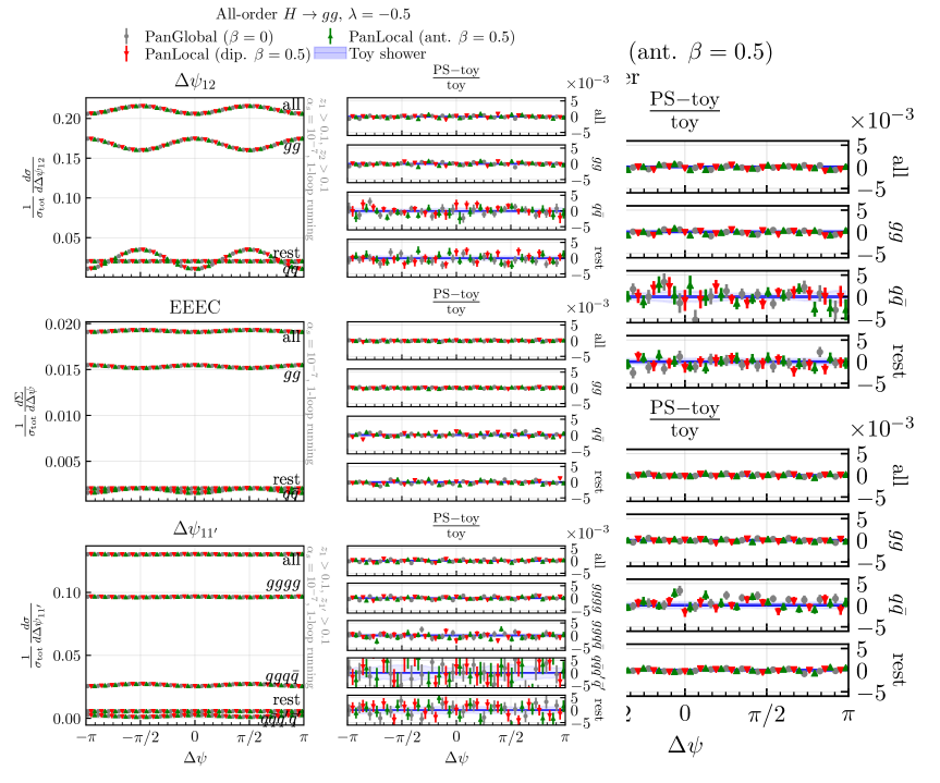
Figure 18: All-order comparison of the toy shower and different PanScales showers, for $H\to gg$ events. The three observables shown here are the azimuthal angle between a primary and secondary splitting plane $\Delta\psi_{12}$, the EEEC, and the azimuthal angle between two primary splittings (on opposite sides of the event) $\Delta\psi_{11^{\prime}}$.

4.3 Phenomenological remarks

We comment on three aspects here that are potentially relevant for phenomenological applications.

flavour channel for 2${}^{\text{nd}}$ splitting	$g\to q\bar{q}$	$g\to gg$	all
EEEC	-0.36	0.026	-0.008
$\Delta\psi_{12}$, $z_{1},z_{2}>0.1$	-0.61	0.050	-0.025
$\Delta\psi_{12}$, $z_{1}>0.1$, $z_{2}>0.3$	-0.81	0.086	-0.042

Table 3: The relative magnitude of the azimuthal modulation, $a_{2}/a_{0}$ (cf. Eq. (11)), for the EEEC and Lund intra-jet $\Delta\psi_{12}$ observables, the latter for two sets of cuts on $z_{1}$ and $z_{2}$. The results are shown for $\gamma^{*}\to q\bar{q}$ events for $n_{f}=5$, separately for two specific flavour channels, as well as the sum over all flavour channels (including the channel without spin correlations, $q\to qg$). As in Fig. 17, the results are obtained in the limit $\alpha_{s}\to 0$ for fixed $\lambda=\alpha_{s}L=-0.5$ and for the Lund declustering $\Delta\psi_{12}$ we consider events with $k_{t,2}/Q>e^{-|L|}$, while for the EEEC $\Delta\psi$ we consider events with $\theta_{S}>e^{-|L|}$.

Our first comment concerns the relative size of spin correlations in the EEEC and the $\Delta\psi_{12}$ Lund declustering observable. The EEEC has the advantage of not requiring a $z_{\text{cut}}$, reducing the number of parameters that need to be chosen for the observable. However its weighting with the energies in Eq. (12) tends to favour configurations where a $q\to qg(g\to xy)$ splitting shares energy equally between the three final particles. In the notation of Figs. 4 and 5, this corresponds to $z_{1}\simeq 2/3$ and $z_{2}\simeq 1/2$. While $z_{2}\simeq 1/2$ acts to enhance the spin correlations, $z_{1}\simeq 2/3$ tends to reduce them. In contrast, with the Lund declustering $\Delta\psi_{12}$ one can adjust the cuts on the $z_{1}$ and $z_{2}$ values so as to maximise the azimuthal modulations. Table 3 summarises the degree of azimuthal modulation for different observables in $\gamma^{*}\to q\bar{q}$ events. With our default (non-optimised) cuts of $z_{1}$ and $z_{2}>0.1$, we see substantially larger azimuthal modulations than in the EEEC variables, both in individual flavour channels and in their sum. The potential for further enhancement of the modulations is made evident by the results obtained with the $z_{2}>0.3$ requirement.

Our second comment concerns the sum over all flavour channels. The results shown here have been obtained with $n_{f}=5$ light flavours. The final magnitude of the spin correlations after the sum over flavour channels is quite sensitive to the cancellation between $g\to q\bar{q}$ and $g\to gg$ splittings and the degree of cancellation is strongly influenced by the value of $n_{f}$. At the scales where one might aim to probe spin correlations, the $c$- and especially $b$-quark masses are not entirely negligible. A full phenomenological study of the flavour-summed structure of azimuthal correlations might, therefore, needs to take into account finite quark-mass effects. Note that effects related to $k_{t}$ values in the neighbourhood of a heavy-quark threshold are formally suppressed by a logarithm. For a complete understanding of phenomenological expectations one would also want to examine the impact of other subleading logarithmic effects, as well as contributions suppressed by powers of $k_{t}/Q$, and possibly also non-perturbative corrections. It would clearly also be of interest to find ways of carrying out measurements with flavour tagging, given the strong effects to be seen with $g\to q\bar{q}$ splittings. While $b$ and $c$ flavour tagging are the most obviously robust starting points in this respect, one may also wish to consider $s$ tagging [61] and generic light-quark versus gluon discrimination observables.

Our final comment concerns the inter-jet $\Delta\psi_{11^{\prime}}$ observable. If Higgs boson decay to two gluons is eventually observed and if one can carry out flavour tagging so as to have visible net modulation, this observable could provide an interesting example of an EPR type measurement at colliders (a constraint on a gluon’s splitting angle would then translate to a constraint on the distance travelled by the gluon before it splits).

5 Conclusions

The developments shown in this paper are among the last remaining aspects needed in order to claim complete NLL accuracy in the sense of Ref. [24] for the PanScales family of parton showers. The one component that now remains (at leading colour) is a treatment of the spin correlations for soft emissions, an aspect that we leave to future work.

The approach we have taken is largely based on that proposed by Collins and Knowles, and in part also on the extension to dipole showers proposed by Richardson and Webster. The main difference relative to the Richardson and Webster work is our use of spinor products, avoiding the need for correlating branching variables across different steps and associated boosts. The spin correlation treatment is then expected to be correct at single-logarithmic accuracy for showers that adhere to the general requirements set out in Ref. [24].

Relative to earlier work on spin correlations in parton showers, one of the main novelties of this paper is the framework for validating the implementation of spin correlations. As part of our testing framework we extended the MicroJets code to enable single-logarithmic resummation for a range of spin-correlation observables. Figures 13–16 show clear agreement between the collinear limits of fixed-order matrix elements and a fixed-order expansion of the shower, while Figs. 17 and 18 show equally good agreement between the logarithmic structure of the full shower and the single-logarithmic resummed expectations.

To carry out those tests we introduced a set of new observables based on Lund declustering that are sensitive to spin correlations. These complement the recently proposed EEEC spin-sensitive observables, providing information that is more differential in momentum fractions of the different branchings. This makes it possible to enhance the relative magnitude of the spin-correlation signal, cf. Table 3. Spin-correlation effects can be large for $g\to q{\bar{q}}$ splittings, while they are smaller, with an opposite sign for $g\to gg$ splittings (cf. Figs. 4–6). All-order resummation has a modest effect on them (cf. Figs. 9–11). Phenomenologically, the opposite signs for $g\to gg$ and $g\to q{\bar{q}}$ lead to a partial cancellation of the spin correlation effects in flavour-insensitive observables, although our studies indicate that some effect remains visible. Further study of the potential for measuring these effects, possibly in combination with flavour tagging, would clearly be of interest.

Appendix A Deriving the branching amplitudes

In this appendix we collect some details regarding the computation of branching amplitudes in terms of spinor products and their numerical evaluation. The calculations here are done following the conventions of Ref. [62]. For two light-like momenta $p$ and $q$, we define the spinor product

$$S_{\lambda}(p,q)=\bar{u}_{\lambda}(p)u_{-\lambda}(q),$$ (25)

where $\lambda=\pm 1$ is the Dirac spinor helicity. Spinor products have the properties

$$S_{\lambda}(p,q)=-S_{\lambda}(q,p)=-S_{-\lambda}(p,q)^{*},$$

$$|S_{\lambda}(p,q)|^{2}=S_{\lambda}(p,q)S_{-\lambda}(q,p)=2\,p{\cdot}q.$$ (26a)

Following the HELAS conventions [63], the polarisation vector of a gluon with momentum $p$ is defined as

$$\epsilon^{*\mu}_{\lambda}(p)=\frac{1}{\sqrt{2}}\frac{1}{S_{-\lambda}(r,p)}\bar{u}_{\lambda}(p)\gamma^{\mu}u_{\lambda}(r),$$ (27)

where $r$ is a light-like vector specifying the gauge. For calculational purposes, the Chisholm identity [62]

$$\not{\epsilon}^{*}_{\lambda}(p)=\frac{\sqrt{2}}{S_{-\lambda}(r,p)}\bigg{[}u_{\lambda}(r)\bar{u}_{\lambda}(p)+u_{-\lambda}(p)\bar{u}_{-\lambda}(r)\bigg{]}$$ (28)

is often useful. We define the momenta of a collinear splitting as $p_{a}\rightarrow p_{b}+p_{c}$, such that $p_{b}=zp_{a}$ and $p_{c}=(1-z)p_{a}$. In this limit, the gauge vector $r$ cancels from the collinear branching amplitudes, and they may be written in terms of a single spinor product $S_{\lambda}(p_{b},p_{c})$ using the identities

$$S_{\lambda}(p_{b},p_{a})=\sqrt{1-z}S_{\lambda}(p_{b},p_{c})\text{ and }S_{\lambda}(p_{c},p_{a})=-\sqrt{z}S_{\lambda}(p_{b},p_{c}).$$ (29)

Next, we compute the branching amplitudes for all colour-stripped collinear QCD branchings, dropping any overall phase factors for convenience.

$q\rightarrow qg$

The branching amplitude is

$$\mathcal{M}_{a\to bc}^{\lambda_{a}\lambda_{b}\lambda_{c}} =\frac{g_{s}}{2p_{b}{\cdot}p_{c}}\bar{u}_{\lambda_{b}}(p_{b})\not{\epsilon}^{*}_{\lambda_{c}}(p_{c})u_{\lambda_{a}}(p_{a})$$ (30a)

$$=\frac{1}{\sqrt{2}}\frac{g_{s}}{p_{b}{\cdot}p_{c}}\frac{1}{S_{-\lambda_{c}}(r,p_{c})}\bar{u}_{\lambda_{b}}(p_{b})\Big{[}u_{\lambda_{j}}(r)\bar{u}_{\lambda_{c}}(p_{c})+u_{-\lambda_{c}}(p_{c})\bar{u}_{-\lambda_{j}}(r)\Big{]}u_{\lambda_{a}}(p_{a}).$$ (30b)

The non-zero helicity configurations are

$$\mathcal{M}_{a\to bc}^{\lambda,\lambda,\lambda} =\frac{1}{\sqrt{2}}\frac{g_{s}}{p_{b}{\cdot}p_{c}}\frac{1}{\sqrt{1-z}}S_{\lambda}(p_{b},p_{c}),$$ (31a)

$$\mathcal{M}_{a\to bc}^{\lambda,\lambda,-\lambda} =\frac{1}{\sqrt{2}}\frac{g_{s}}{p_{b}{\cdot}p_{c}}\frac{z}{\sqrt{1-z}}S_{-\lambda}(p_{b},p_{c}).$$ (31b)

$g\rightarrow q\bar{q}$

The branching amplitude is

$$\mathcal{M}_{a\to bc}^{\lambda_{a}\lambda_{b}\lambda_{c}} =\frac{g_{s}}{2p_{b}{\cdot}p_{c}}\bar{u}_{\lambda_{b}}(p_{b})\not{\epsilon}^{*}_{-\lambda_{a}}(p_{a})u_{-\lambda_{c}}(p_{c})$$ (32a)

$$=\frac{1}{\sqrt{2}}\frac{g_{s}}{p_{b}{\cdot}p_{c}}\frac{1}{S_{\lambda_{a}}(r,p_{a})}\bar{u}_{\lambda_{b}}(p_{b})\bigg{[}u_{-\lambda_{a}}(r)\bar{u}_{-\lambda_{a}}(p_{a})+u_{\lambda_{a}}(p_{a})\bar{u}_{\lambda_{a}}(r)\bigg{]}u_{-\lambda_{c}}(p_{c}).$$ (32b)

The non-zero helicity configurations are

$$\mathcal{M}_{a\to bc}^{\lambda,\lambda,-\lambda} =-\frac{1}{\sqrt{2}}\frac{g_{s}}{p_{b}{\cdot}p_{c}}zS_{-\lambda}(p_{b},p_{c}),$$ (33a)

$$\mathcal{M}_{a\to bc}^{\lambda,-\lambda,\lambda} =\frac{1}{\sqrt{2}}\frac{g_{s}}{p_{b}{\cdot}p_{c}}(1-z)S_{-\lambda}(p_{b},p_{c}).$$ (33b)

$g\rightarrow gg$

For this case, we first derive some general properties. If we consider the collinear limit and pick all gluons to have the same gauge vector $r$, we find

$$\epsilon^{*}_{\lambda}(p_{i}){\cdot}\epsilon^{*}_{\lambda}(p_{j}) =0,$$ (34a)

$$\epsilon^{*}_{\lambda}(p_{i}){\cdot}\epsilon^{*}_{-\lambda}(p_{j}) =1,$$ (34b)

$$\epsilon^{*}_{\lambda}(p_{i}){\cdot}p_{j} =\frac{1}{\sqrt{2}}\frac{S_{-\lambda}(p_{j},r)}{S_{-\lambda}(r,p_{i})}S_{\lambda}(p_{i},p_{j}),$$ (34c)

where $p_{i},p_{j}\in\{p_{a},p_{b},p_{c}\}$. The branching amplitude is

$$\mathcal{M}_{a\to bc}^{\lambda_{a}\lambda_{b}\lambda_{c}} =-\frac{g_{s}}{p_{b}{\cdot}p_{c}}\Big{(}\epsilon^{*}_{\lambda_{b}}(p_{b}){\cdot}p_{c}\,\epsilon^{*}_{\lambda_{c}}(p_{c}){\cdot}\epsilon^{*}_{-\lambda_{a}}(p_{a})-\epsilon^{*}_{\lambda_{c}}(p_{c}){\cdot}p_{b}\,\epsilon^{*}_{\lambda_{b}}(p_{b}){\cdot}\epsilon^{*}_{-\lambda_{a}}(p_{a})$$

$$+\epsilon^{*}_{-\lambda_{a}}(p_{a}){\cdot}p_{b}\,\epsilon^{*}_{\lambda_{b}}(p_{b}){\cdot}\epsilon^{*}_{\lambda_{c}}(p_{c})\Big{)}.$$ (35)

The non-zero helicity configurations are

$$\mathcal{M}_{a\to bc}^{\lambda,\lambda,\lambda} =\frac{1}{\sqrt{2}}\frac{g_{s}}{p_{b}{\cdot}p_{c}}\frac{1}{\sqrt{z(1-z)}}S_{\lambda}(p_{b},p_{c}),$$ (36a)

$$\mathcal{M}_{a\to bc}^{\lambda,\lambda,-\lambda} =\frac{1}{\sqrt{2}}\frac{g_{s}}{p_{b}{\cdot}p_{c}}\frac{z^{3/2}}{\sqrt{1-z}}S_{-\lambda}(p_{b},p_{c}),$$ (36b)

$$\mathcal{M}_{a\to bc}^{\lambda,-\lambda,\lambda} =\frac{1}{\sqrt{2}}\frac{g_{s}}{p_{b}{\cdot}p_{c}}\frac{(1-z)^{3/2}}{\sqrt{z}}S_{-\lambda}(p_{b},p_{c}).$$ (36c)

Numerical evaluation of spinor products

To find an expression for the spinor product that can be evaluated numerically, we may introduce arbitrary reference vectors $k_{0}$ and $k_{1}$ which obey $k_{0}^{2}=0$, $k_{1}^{2}=-1$ and $k_{0}{\cdot}k_{1}=0$. Then, without loss of generality, we may write

$$u_{+}(p)=\frac{1}{\sqrt{2p{\cdot}k_{0}}}\not{p}u_{-}(k_{0})\text{ and }u_{-}(p)=\frac{1}{\sqrt{2p{\cdot}k_{0}}}\not{p}\not{k}_{1}u_{-}(k_{0}).$$ (37)

The spinor product may then be expressed as

$$S_{+}(p_{b},p_{c}) =\frac{1}{\sqrt{2p_{b}{\cdot}k_{0}}\sqrt{2p_{c}{\cdot}k_{0}}}\bar{u}_{-}(k_{0})\not{k}_{1}\not{p}_{b}\not{p}_{c}u_{-}(k_{0})$$ (38a)

$$=\frac{1}{2}\frac{1}{\sqrt{2p_{b}{\cdot}k_{0}}\sqrt{2p_{c}{\cdot}k_{0}}}\textrm{tr}\left((1-\gamma^{5})\not{k}_{0}\not{k}_{1}\not{p}_{b}\not{p}_{c}\right)$$ (38b)

$$=\frac{1}{\sqrt{p_{b}{\cdot}k_{0}}\sqrt{p_{c}{\cdot}k_{0}}}\bigg{[}(p_{c}{\cdot}k_{0})(p_{b}{\cdot}k_{1})-(p_{b}{\cdot}k_{0})(p_{c}{\cdot}k_{1})-i\epsilon_{\mu\nu\alpha\beta}k_{0}^{\mu}k_{1}^{\nu}p_{b}^{\alpha}p_{c}^{\beta}\bigg{]}.$$ (38c)

While this expression remains independent of a choice of representation of the Dirac algebra, an explicit choice for the reference vectors $k_{0}$ and $k_{1}$ must be made for the purposes of numerical evaluation. For instance, if we choose $k_{0}=(1,0,0,-1)$ and $k_{1}=(0,1,0,0)$, we find

$$S_{+}(p_{b},p_{c}) =\sqrt{\frac{p_{c}^{0}+p_{c}^{3}}{p_{b}^{0}+p_{b}^{3}}}(p_{b}^{1}+ip_{b}^{2})-\sqrt{\frac{p_{b}^{0}+p_{b}^{3}}{p_{c}^{0}+p_{c}^{3}}}(p_{c}^{1}+ip_{c}^{2}).$$ (39)

In the shower implementation, reference vectors are selected on an event-by-event basis, where care is taken not to select a direction that aligns with the initial momenta to avoid numerical instabilities.

Appendix B An example of calculating the functions $A(z)$, $B(z)$

We illustrate the computation of the spin-correlated matrix element squared, taking the example of the observable $\Delta\psi_{12}$ at second order for a quark-initiated jet, $q\to qg(g\to q^{\prime}\bar{q}^{\prime})$, of Fig. 1. We then cast the result into the form of Eq. (11). The matrix element squared, summing over all helicities, is given by

$$|M|^{2} =\mathcal{M}_{0\to 12}^{\lambda_{0}\lambda_{1}\lambda_{2}}\mathcal{M}_{0\to 12}^{*\lambda_{0}\lambda_{1}\lambda_{2}^{\prime}}\mathcal{M}_{2\to 34}^{\lambda_{2}\lambda_{3}\lambda_{4}}\mathcal{M}_{2\to 34}^{*\lambda_{2}^{\prime}\lambda_{3}\lambda_{4}}$$

$$=\mathcal{M}_{0\to 12}^{+++}\mathcal{M}_{0\to 12}^{*+++}(\mathcal{M}_{2\to 34}^{++-}\mathcal{M}_{2\to 34}^{*++-}+\mathcal{M}_{2\to 34}^{+-+}\mathcal{M}_{2\to 34}^{*+-+})$$

$$+\mathcal{M}_{0\to 12}^{+++}\mathcal{M}_{0\to 12}^{*++-}(\mathcal{M}_{2\to 34}^{+-+}\mathcal{M}_{2\to 34}^{*--+}+\mathcal{M}_{2\to 34}^{++-}\mathcal{M}_{2\to 34}^{*-+-})$$

$$+\mathcal{M}_{0\to 12}^{++-}\mathcal{M}_{0\to 12}^{*+++}(\mathcal{M}_{2\to 34}^{--+}\mathcal{M}_{2\to 34}^{*+-+}+\mathcal{M}_{2\to 34}^{-+-}\mathcal{M}_{2\to 34}^{*++-})$$

$$+\mathcal{M}_{0\to 12}^{++-}\mathcal{M}_{0\to 12}^{*++-}(\mathcal{M}_{2\to 34}^{-+-}\mathcal{M}_{2\to 34}^{*-+-}+\mathcal{M}_{2\to 34}^{--+}\mathcal{M}_{2\to 34}^{*--+})$$

$$+(+\leftrightarrow-)\,,$$ (40)

where the last line includes the flipping of all helicities, and we have already excluded forbidden helicities. Using Eq. (5) and inserting the functions $\mathcal{F}_{a\to bc}^{\lambda_{a}\lambda_{b}\lambda_{c}}(z)$ given in Table 1, the above reduces to

$$|M|^{2} =2\frac{2g_{s}^{2}}{\theta_{12}^{2}E_{0}^{2}z_{1}(1-z_{1})}\frac{2g_{s}^{2}}{\theta_{34}^{2}E_{2}^{2}z_{2}(1-z_{2})}$$

$$\times\Big{(}\frac{z_{2}^{2}+(1-z_{2})^{2}}{1-z_{1}}-\frac{2z_{1}z_{2}(1-z_{2})}{1-z_{1}}e^{2i(\phi_{1}-\phi_{2})}$$

$$-\frac{2z_{1}z_{2}(1-z_{2})}{1-z_{1}}e^{-2i(\phi_{1}-\phi_{2})}+\frac{z_{1}^{2}((1-z_{2})^{2}+z_{2}^{2})}{1-z_{1}}\Big{)}$$ (41a)

$$=\frac{8g_{s}^{4}(1+z_{1}^{2})(z_{2}^{2}+(1-z_{2})^{2})}{\theta_{12}^{2}\theta_{34}^{2}E_{0}^{4}z_{1}(1-z_{1})^{4}z_{2}(1-z_{2})}\Big{(}1+\frac{2z_{1}}{1+z_{1}^{2}}\frac{-2z_{2}(1-z_{2})}{z_{2}^{2}+(1-z_{2})^{2}}\cos(2\Delta\phi)\Big{)}\,,$$ (41b)

where each of the four terms in the parenthesis of Eq. (41a) comes from one of the four lines in Eq. (40). Finally, Eq. (41b) makes the form of $A(z_{1})$ and $B(z_{2})$ explicit.

Appendix C Rotational invariance in the collinear limit

As part of the numerical evaluation of spinor products in Eq. (39), a set of reference vectors must be selected. Any dependence on these reference vectors vanishes in the calculation of a full squared matrix element, but the Collins-Knowles algorithm only accounts for the contributions that dominate the matrix element in the collinear limit. Consequently, any dependence on the reference vectors should also vanish from the Collins-Knowles result as long as the shower emissions are strongly ordered and sufficiently collinear.

In this appendix, we validate this property in the PanScales implementation of the Collins-Knowles algorithm. To that end, like in section 4.1.1, the Collins-Knowles weight as a function of an angular resolution is considered. Rather than comparing to a matrix element directly, the weight is computed for an event, and for the same event that is rotated randomly. As the reference vectors stay fixed, rotating the event is equivalent to rotating the reference vectors in the original event. Figure 19 shows the relative difference of these weights for two shower emissions off $\gamma^{*}\rightarrow q\bar{q}$ and $H\rightarrow gg$ hard scatterings. The relative difference in weights decreases as a power of the angular resolution, and is thus a power correction that vanishes in the collinear limit. Numerically, these effects are also small compared to the size of the spin correlations themselves.

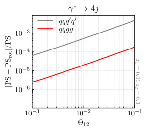
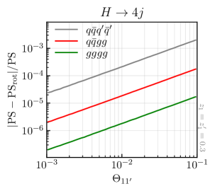
Figure 19: Comparison of the Collins-Knowles weights of two-emission events and their randomly rotated counterpart. The hard scattering is either $\gamma^{*}\rightarrow q\bar{q}$ (left), where a single primary ($z_{1}=0.01$) and secondary emission ($z_{2}=0.3$) are performed, or $H\rightarrow gg$ (right), where two opposite-side primary emissions are performed ($z_{1}=z_{1^{\prime}}=0.3$).

Appendix D Technical details of the all-order comparisons

To facilitate the isolation of the NLL structure of the parton shower, the all-order comparisons of section 4.2 are performed at extremely small values of $\alpha_{s}$ and extremely large values of the logarithm. Several techniques need to be employed to maintain numerically feasible analyses in these extreme regimes. In this appendix we detail these techniques.

D.1 Removal of soft radiation

The particle multiplicity generated by the parton shower scales like $\sqrt{\alpha_{s}L^{2}}$. This means that, because the product $\alpha_{s}L$ is kept constant as $\alpha_{s}$ decreases and $L$ increases, the multiplicity also increases. At the logarithmic values used in section 4.2, the multiplicity has increased to levels that cause the event generation to become numerically unfeasible. However, the all-order observables considered here are insensitive to soft gluon radiation, and the spin correlations incorporated by the Collins-Knowles algorithm are also unaffected. As a result, as long as any radiation that is removed is sufficiently soft that its recoil has no noticeable impact on the momenta of the partons that dominate the Lund declustering and energy-correlator observables, the all-order tests should remain unaffected by the removal of soft gluon radiation. Such a cut is implemented in the PanScales shower by limiting the sampling range of the auxiliary parton shower variable that controls the collinear momentum fraction. This strategy is more efficient than the alternative of vetoing soft branchings, as the shower would spend much of its time generating and vetoing soft emissions at low scales. An illustration of this procedure is shown in Fig. 20.

Figure 20: An example of the shower Lund plane after the first branching, with a cut on soft emissions. The red shaded area indicates the part of phase space removed by the soft-emission cut, which is applied relative to the total event energy. The black dashed line represents a possible observable cut on $z$, such as that applied by the Lund declustering observables. It is applied relative to the parent momentum. To avoid removing parts of the phase space above the dashed line due to recoil effects, the soft-emission cut is applied well below the observable cut.

To validate the legitimacy of the application of this cut on soft radiation, we compare the predictions of the PanScales showers and our implementation of Dire v1 for $\Delta\psi_{12}$ with $z_{\text{cut}}=0.1$ at $\alpha_{s}=0.01$ and $L=-27.5$. Figure 21 shows the difference between the distributions with and without the application of the collinear cut $\ln z>\ln z_{\text{cut}}^{\text{PS}}=-10$. This value of $z_{\text{cut}}^{\text{PS}}$ is significantly below the $z$ values that dominate in our observables. For the PanScales showers, we see that the cut has no statistically significant effect on the azimuthal distribution and thus we conclude that we can safely use a $z_{\text{cut}}^{\text{PS}}$ in our logarithmic accuracy tests. For other showers, the cut can have an impact on the results, as illustrated with the Dire v1 dipole shower, where the cut induces a change in $a_{2}$ that is a significant fraction of the actual $a_{2}$. We attribute this to transverse recoil effects between gluons of commensurate $k_{t}$ values, of the kind discussed in Refs. [23, 24]. For such showers, a test of the logarithmic structure of the spin correlations would need to be carried out without a $z_{\text{cut}}^{\text{PS}}$. We suspect that there are observables for which such tests would reveal problems in the $\alpha_{s}^{n}L^{n}$ logarithmic structure, associated with the following type of configuration: consider a hard-collinear $g\to q\bar{q}$ splitting with a transverse momentum $k_{t,1}$, followed by a soft-collinear emission with transverse momentum $k_{t,2}\lesssim k_{t,1}$ from the dipole that contains the $q$. Within standard dipole-shower recoil schemes, the soft-collinear emission can take its recoil from the quark, altering its 2-dimensional vector transverse momentum, effectively smearing out the azimuthal angle of the $q\bar{q}$ pair. In certain circumstances (for example if one considers events where the $g\to q\bar{q}$ splitting is the highest-$k_{t}$ splitting in the event), the product of squared-matrix element and phase space where the recoil can occur will lead to a factor $\alpha_{s}L$ for this smearing to occur, thus spoiling single-logarithmic accuracy. Note, however, that in the observables that we actually consider, we do not require either of the collinear splittings to be the hardest in the event, and we expect that feature to bring further complications, of the kind discussed in section 3 of the supplemental material of Ref. [24], whereby additional double-logarithmic effects would be expected to (at least) partially mask these issues in the all-order tests, potentially associated with super-leading logarithms, $\alpha_{s}^{n}L^{m}$ with $m>n$, for observables that should only have $m\leq n$. Based on these arguments, we consider the presence of any effect from emissions below $z_{\text{cut}}$, as seen in Fig. 21, to be a sign of potential danger.

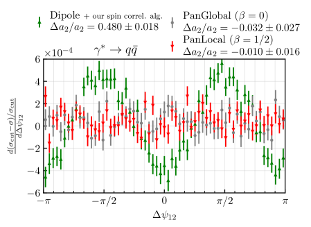
Figure 21: Difference in the $\Delta\psi_{12}$ distribution between a run with a collinear cut $\ln z_{\text{cut}}^{\text{PS}}=-10$ and a run without. The results are shown for finite $\alpha_{s}=0.01$ and $L=-27.5$, and three showers. The key also shows the result for $\Delta a_{2}/a_{2}$ where $\Delta a_{2}$ is the difference between the $a_{2}$ Fourier coefficient as obtained with and without the cut. The result labelled “Dipole” corresponds to our implementation of the Dire v1 [64] shower algorithm supplemented with our spin-correlation algorithm and we expect it to be representative of a variety of standard dipole-type showers. It indicates that the use of a $\ln z_{\text{cut}}$ would not be safe for testing spin correlations in such standard dipole-type showers.

D.2 Stand-in observables

While performing tests at small $\alpha_{s}$ and large logarithms, it quickly becomes challenging to accurately evaluate the tiny angles between collinear momenta. To avoid large numerical cancellations in the evaluation of inner products, the PanScales showers have the option to explicitly track the difference in direction between dipole components. This technique, as well as the use of a new floating-point type (double_exp) that increases the maximum size of the exponent of a regular double-precision type, was already used in [25], and was equally crucial for the all-order tests performed here. While it allows the shower to be run at asymptotically small values of the coupling, the evaluation of the observables is not as straightforward.

In the case of Lund-declustering observables, a regular analysis is technically limited by the absence of directional difference information for parton pairs that are not in the same dipoles. In events with at most a Born $q\bar{q}$ pair, we have implemented functionality whereby we use the full dipole chain and in-dipole direction differences to construct a look-up table for the direction differences between any pair of partons. For $N$ particles this has an $\mathcal{O}\left(N^{2}\right)$ time and memory cost, while normal $e^{+}e^{-}$ clustering in FastJet also carries an $\mathcal{O}\left(N^{2}\right)$ time cost, but an $\mathcal{O}\left(N\right)$ memory cost. Used together with a winner-takes-all recombination scheme [65, 66, 67] in a version of the FastJet [68] code adapted to work with the double_exp type, we can carry out the Lund declustering analysis at asymptotic values of the logarithm. However the current technical limitation of having at most the Born $q\bar{q}$ pair in the event means that we need an alternative strategy for complete events.

Accordingly, we have developed a stand-in analysis that uses the binary tree generated by the Collins-Knowles algorithm, even though it is normally unobservable. During the showering, the Lund structure is determined using explicit shower information, where at every collinear branching that appears in the binary tree, the appropriate azimuthal information is stored if the collinear momentum fraction cuts are passed. This procedure is equivalent to the evaluation of the exact observable if the jet clustering produces the same binary tree (for the hard emissions that we ultimately consider in the observable) as in our implementation of the Collins-Knowles algorithm and if recoil effects that can affect the momentum fraction cuts are absent. At asymptotically small $\alpha_{s}$, for the subset of PanScales showers that passed the NLL tests in Ref. [24], and with the condition that one works with a hardness cut $z>z_{\text{cut}}$ such that $\alpha_{s}\ln z_{\text{cut}}\ll 1$, these are both valid assumptions. We have verified this by considering events without $g\to q\bar{q}$ splittings and establishing that the full Lund declustering and the stand-in analysis produced event-by-event identical results. Note that the stand-in analysis also allows easy access to the flavour separation of the spin-correlation effects, without the need to consider flavoured jet clustering.

In the case of the EEEC, a major issue it its $\mathcal{O}(N^{3})$ time complexity, which quickly becomes prohibitive at the multiplicities under consideration. The following procedure, which again makes direct use of the binary tree, is again equivalent to the full observable in the asymptotic limit. For all nodes $a_{n}$ that are not terminal, and where $n$ is the depth of that node, do as follows:

1. Retrieve the opening angle $\theta_{S}$ and the normal vector $\vec{n}_{S}$ of the branching of node $a_{n}$.

2. Retrieve the global momentum fractions $z_{1}=2E_{1}/Q$, $z_{2}=2E_{2}/Q$ of the outgoing momenta $1$ and $2$ of node $a_{n}$.

3. Iteratively for $i\in\{1,..,n-1\}$:

   • Retrieve the opening angle $\theta_{L}$ and the normal vector $\vec{n}_{L}$ of the branching of node $a_{i}$.

   • Retrieve the global momentum fraction $z_{3}=E_{3}/2E_{\mathrm{CM}}$, where $3$ is the outgoing momentum of $a_{i}$ that is not $a_{i+1}$.

   • Compute the signed angle $\Delta\psi$ between $\vec{n}_{S}$ and $\vec{n}_{L}$.

   • Add to the $\Delta\psi$-$\theta_{S}$-$\theta_{L}$-bin with weight $2z_{1}z_{2}z_{3}$.

This procedure has time-complexity $\mathcal{O}(N\log N)$ and is again equivalent to the exact observable if $\theta_{S}\ll\theta_{L}$ and in the absence of recoil effects, which are both the case for asymptotically small $\alpha_{s}$ for the showers we study. The above algorithm was validated by verifying that it yields identical results to the exact observable evaluation for a representative number of events.

References

- [1] A. Einstein, B. Podolsky, and N. Rosen, Can quantum mechanical description of physical reality be considered complete? Phys. Rev. 47 (1935) 777–780.
- [2] G. Mahlon and S. J. Parke, Angular correlations in top quark pair production and decay at hadron colliders. Phys. Rev. D 53 (1996) 4886–4896, arXiv:hep-ph/9512264.
- [3] W. Bernreuther, A. Brandenburg, Z. G. Si, and P. Uwer, Top quark spin correlations at hadron colliders: Predictions at next-to-leading order QCD. Phys. Rev. Lett. 87 (2001) 242002, arXiv:hep-ph/0107086.
- [4] W. Bernreuther and Z.-G. Si, Distributions and correlations for top quark pair production and decay at the Tevatron and LHC. Nucl. Phys. B 837 (2010) 90–121, arXiv:1003.3926 [hep-ph].
- [5] G. Mahlon and S. J. Parke, Spin Correlation Effects in Top Quark Pair Production at the LHC. Phys. Rev. D 81 (2010) 074024, arXiv:1001.3422 [hep-ph].
- [6] K. Melnikov and M. Schulze, Top quark spin correlations at the Tevatron and the LHC. Phys. Lett. B 700 (2011) 17–20, arXiv:1103.2122 [hep-ph].
- [7] P. Artoisenet, R. Frederix, O. Mattelaer, and R. Rietkerk, Automatic spin-entangled decays of heavy resonances in Monte Carlo simulations. JHEP 03 (2013) 015, arXiv:1212.3460 [hep-ph].
- [8] ATLAS Collaboration, G. Aad et al., Observation of spin correlation in events from pp collisions at sqrt(s) = 7 TeV using the ATLAS detector. Phys. Rev. Lett. 108 (2012) 212001, arXiv:1203.4081 [hep-ex].
- [9] ATLAS Collaboration, G. Aad et al., Measurement of Top Quark Polarization in Top-Antitop Events from Proton-Proton Collisions at = 7 TeV Using the ATLAS Detector. Phys. Rev. Lett. 111 (2013) no. 23, 232002, arXiv:1307.6511 [hep-ex].
- [10] CMS Collaboration, S. Chatrchyan et al., Measurements of Spin Correlations and Top-Quark Polarization Using Dilepton Final States in Collisions at = 7 TeV. Phys. Rev. Lett. 112 (2014) no. 18, 182001, arXiv:1311.3924 [hep-ex].
- [11] ATLAS Collaboration, G. Aad et al., Measurements of spin correlation in top-antitop quark events from proton-proton collisions at TeV using the ATLAS detector. Phys. Rev. D 90 (2014) no. 11, 112016, arXiv:1407.4314 [hep-ex].
- [12] ATLAS Collaboration, G. Aad et al., Measurement of Spin Correlation in Top-Antitop Quark Events and Search for Top Squark Pair Production in pp Collisions at TeV Using the ATLAS Detector. Phys. Rev. Lett. 114 (2015) no. 14, 142001, arXiv:1412.4742 [hep-ex].
- [13] W. Bernreuther, D. Heisler, and Z.-G. Si, A set of top quark spin correlation and polarization observables for the LHC: Standard Model predictions and new physics contributions. JHEP 12 (2015) 026, arXiv:1508.05271 [hep-ph].
- [14] CMS Collaboration, A. M. Sirunyan et al., Measurement of the top quark polarization and spin correlations using dilepton final states in proton-proton collisions at 13 TeV. Phys. Rev. D 100 (2019) no. 7, 072002, arXiv:1907.03729 [hep-ex].
- [15] A. Behring, M. Czakon, A. Mitov, A. S. Papanastasiou, and R. Poncelet, Higher order corrections to spin correlations in top quark pair production at the LHC. Phys. Rev. Lett. 123 (2019) no. 8, 082001, arXiv:1901.05407 [hep-ph].
- [16] Y. Afik and J. R. M. de Nova, Quantum information and entanglement with top quarks at the LHC. arXiv:2003.02280 [quant-ph].
- [17] M. Fabbrichesi, R. Floreanini, and G. Panizzo, Testing Bell inequalities at the LHC with top-quark pairs. arXiv:2102.11883 [hep-ph].
- [18] ALEPH Collaboration, R. Barate et al., A Measurement of the QCD color factors and a limit on the light gluino. Z. Phys. C 76 (1997) 1–14.
- [19] S. Moretti and W. J. Stirling, Spin correlations in e+ e- — four jets. Eur. Phys. J. C 9 (1999) 81–93, arXiv:hep-ph/9808429.
- [20] B. R. Webber, Monte Carlo Simulation of Hard Hadronic Processes. Ann. Rev. Nucl. Part. Sci. 36 (1986) 253–286.
- [21] J. C. Collins, Spin Correlations in Monte Carlo Event Generators. Nucl. Phys. B304 (1988) 794–804.
- [22] I. Knowles, Angular Correlations in QCD. Nucl. Phys. B 304 (1988) 767–793.
- [23] M. Dasgupta, F. A. Dreyer, K. Hamilton, P. F. Monni, and G. P. Salam, Logarithmic accuracy of parton showers: a fixed-order study. JHEP 09 (2018) 033, arXiv:1805.09327 [hep-ph].
- [24] M. Dasgupta, F. A. Dreyer, K. Hamilton, P. F. Monni, G. P. Salam, and G. Soyez, Parton showers beyond leading logarithmic accuracy. Phys. Rev. Lett. 125 (2020) no. 5, 052002, arXiv:2002.11114 [hep-ph].
- [25] K. Hamilton, R. Medves, G. P. Salam, L. Scyboz, and G. Soyez, Colour and logarithmic accuracy in final-state parton showers. JHEP 03 (2021) 041, arXiv:2011.10054 [hep-ph].
- [26] B. Andersson, G. Gustafson, L. Lonnblad, and U. Pettersson, Coherence Effects in Deep Inelastic Scattering. Z. Phys. C43 (1989) 625.
- [27] S. Catani, L. Trentadue, G. Turnock, and B. R. Webber, Resummation of large logarithms in e+ e- event shape distributions. Nucl. Phys. B407 (1993) 3–42.
- [28] G. Corcella, I. G. Knowles, G. Marchesini, S. Moretti, K. Odagiri, P. Richardson, M. H. Seymour, and B. R. Webber, HERWIG 6: An Event generator for hadron emission reactions with interfering gluons (including supersymmetric processes). JHEP 01 (2001) 010, arXiv:hep-ph/0011363 [hep-ph].
- [29] M. Bahr et al., Herwig++ Physics and Manual. Eur. Phys. J. C58 (2008) 639–707, arXiv:0803.0883 [hep-ph].
- [30] J. Bellm et al., Herwig 7.0/Herwig++ 3.0 release note. Eur. Phys. J. C76 (2016) no. 4, 196, arXiv:1512.01178 [hep-ph].
- [31] J. Bellm et al., Herwig 7.2 release note. Eur. Phys. J. C 80 (2020) no. 5, 452, arXiv:1912.06509 [hep-ph].
- [32] P. Richardson and S. Webster, Spin Correlations in Parton Shower Simulations. Eur. Phys. J. C80 (2020) no. 2, 83, arXiv:1807.01955 [hep-ph].
- [33] S. J. Webster, Improved Monte Carlo Simulations of Massive Quarks. PhD thesis, Durham U., 2019.
- [34] Z. Nagy and D. E. Soper, Parton showers with quantum interference. JHEP 09 (2007) 114, arXiv:0706.0017 [hep-ph].
- [35] Z. Nagy and D. E. Soper, Parton showers with quantum interference: Leading color, with spin. JHEP 07 (2008) 025, arXiv:0805.0216 [hep-ph].
- [36] J. R. Forshaw, J. Holguin, and S. Plätzer, Parton branching at amplitude level. JHEP 08 (2019) 145, arXiv:1905.08686 [hep-ph].
- [37] J. R. Forshaw, J. Holguin, and S. Plätzer, Building a consistent parton shower. JHEP 09 (2020) 014, arXiv:2003.06400 [hep-ph].
- [38] H. Chen, I. Moult, and H. X. Zhu, Quantum Interference in Jet Substructure from Spinning Gluons. Phys. Rev. Lett. 126 (2021) no. 11, 112003, arXiv:2011.02492 [hep-ph].
- [39] M. Dasgupta, F. Dreyer, G. P. Salam, and G. Soyez, Small-radius jets to all orders in QCD. JHEP 04 (2015) 039, arXiv:1411.5182 [hep-ph].
- [40] M. Dasgupta, F. A. Dreyer, G. P. Salam, and G. Soyez, Inclusive jet spectrum for small-radius jets. JHEP 06 (2016) 057, arXiv:1602.01110 [hep-ph].
- [41] I. Knowles, Spin Correlations in Parton - Parton Scattering. Nucl. Phys. B 310 (1988) 571–588.
- [42] I. G. Knowles, A Linear Algorithm for Calculating Spin Correlations in Hadronic Collisions. Comput. Phys. Commun. 58 (1990) 271–284.
- [43] P. Richardson, Spin correlations in Monte Carlo simulations. JHEP 11 (2001) 029, arXiv:hep-ph/0110108.
- [44] F. A. Dreyer, G. P. Salam, and G. Soyez, The Lund Jet Plane. JHEP 12 (2018) 064, arXiv:1807.04758 [hep-ph].
- [45] Y. L. Dokshitzer, G. D. Leder, S. Moretti, and B. R. Webber, Better jet clustering algorithms. JHEP 08 (1997) 001, arXiv:hep-ph/9707323 [hep-ph].
- [46] M. Wobisch and T. Wengler, “Hadronization corrections to jet cross-sections in deep inelastic scattering,” in Workshop on Monte Carlo Generators for HERA Physics (Plenary Starting Meeting), pp. 270–279. 1998. arXiv:hep-ph/9907280.
- [47] M. Dasgupta, A. Fregoso, S. Marzani, and G. P. Salam, Towards an understanding of jet substructure. JHEP 09 (2013) 029, arXiv:1307.0007 [hep-ph].
- [48] A. J. Larkoski, S. Marzani, G. Soyez, and J. Thaler, Soft Drop. JHEP 05 (2014) 146, arXiv:1402.2657 [hep-ph].
- [49] Y. Mehtar-Tani, A. Soto-Ontoso, and K. Tywoniuk, Dynamical grooming of QCD jets. Phys. Rev. D 101 (2020) no. 3, 034004, arXiv:1911.00375 [hep-ph].
- [50] P. Caucal, A. Soto-Ontoso, and A. Takacs, Dynamical Grooming meets LHC data. JHEP 07 (2021) 020, arXiv:2103.06566 [hep-ph].
- [51] D. E. Kaplan, K. Rehermann, M. D. Schwartz, and B. Tweedie, Top Tagging: A Method for Identifying Boosted Hadronically Decaying Top Quarks. Phys. Rev. Lett. 101 (2008) 142001, arXiv:0806.0848 [hep-ph].
- [52] CMS Collaboration, A Cambridge-Aachen (C-A) based Jet Algorithm for boosted top-jet tagging Tech. Rep. CMS-PAS-JME-09-001, 2009.
- [53] CMS Collaboration, Boosted Top Jet Tagging at CMS Tech. Rep. CMS-PAS-JME-13-007, 2014.
- [54] T. Plehn, G. P. Salam, and M. Spannowsky, Fat Jets for a Light Higgs. Phys. Rev. Lett. 104 (2010) 111801, arXiv:0910.5472 [hep-ph].
- [55] T. Plehn, M. Spannowsky, M. Takeuchi, and D. Zerwas, Stop Reconstruction with Tagged Tops. JHEP 10 (2010) 078, arXiv:1006.2833 [hep-ph].
- [56] M. Dasgupta, M. Guzzi, J. Rawling, and G. Soyez, Top tagging : an analytical perspective. JHEP 09 (2018) 170, arXiv:1807.04767 [hep-ph].
- [57] A. Banfi, G. P. Salam, and G. Zanderighi, Infrared safe definition of jet flavor. Eur. Phys. J. C 47 (2006) 113–124, arXiv:hep-ph/0601139.
- [58] H. Chen, M.-X. Luo, I. Moult, T.-Z. Yang, X. Zhang, and H. X. Zhu, Three point energy correlators in the collinear limit: symmetries, dualities and analytic results. JHEP 08 (2020) no. 08, 028, arXiv:1912.11050 [hep-ph].
- [59] M. Dasgupta, F. Dreyer, G. P. Salam, and G. Soyez, https://microjets.hepforge.org/.
- [60] S. D. Badger, E. W. N. Glover, and V. V. Khoze, Recursion relations for gauge theory amplitudes with massive vector bosons and fermions. JHEP 01 (2006) 066, arXiv:hep-th/0507161.
- [61] J. Erdmann, O. Nackenhorst, and S. V. Zeißner, Maximum performance of strange-jet tagging at hadron colliders. arXiv:2011.10736 [hep-ex].
- [62] R. Kleiss and W. Stirling, Spinor Techniques for Calculating p anti-p — W+- / Z0 + Jets. Nucl. Phys. B 262 (1985) 235–262.
- [63] H. Murayama, I. Watanabe, and K. Hagiwara, HELAS: HELicity amplitude subroutines for Feynman diagram evaluations Tech. Rep. KEK-91-11, 1992. https://cp3.irmp.ucl.ac.be/projects/madgraph/attachment/wiki/ManualAndHelp/HELAS_reference.pdf.
- [64] S. Hoeche and S. Prestel, The midpoint between dipole and parton showers. Eur. Phys. J. C75 (2015) no. 9, 461, arXiv:1506.05057 [hep-ph].
- [65] D. Bertolini, T. Chan, and J. Thaler, Jet Observables Without Jet Algorithms. JHEP 04 (2014) 013, arXiv:1310.7584 [hep-ph].
- [66] A. J. Larkoski, D. Neill, and J. Thaler, Jet Shapes with the Broadening Axis. JHEP 04 (2014) 017, arXiv:1401.2158 [hep-ph].
- [67] G. P. Salam , unpublished.
- [68] M. Cacciari, G. P. Salam, and G. Soyez, FastJet User Manual. Eur. Phys. J. C72 (2012) 1896, arXiv:1111.6097 [hep-ph].