Endo-Depth-and-Motion: Reconstruction and Tracking in Endoscopic Videos using Depth Networks and Photometric Constraints

Abstract

Estimating a scene reconstruction and the camera motion from in-body videos is challenging due to several factors, e.g. the deformation of in-body cavities or the lack of texture. In this paper we present Endo-Depth-and-Motion, a pipeline that estimates the 6-degrees-of-freedom camera pose and dense 3D scene models from monocular endoscopic sequences. Our approach leverages recent advances in self-supervised depth networks to generate pseudo-RGBD frames, then tracks the camera pose using photometric residuals and fuses the registered depth maps in a volumetric representation. We present an extensive experimental evaluation in the public dataset Hamlyn, showing high-quality results and comparisons against relevant baselines. We also release all models and code for future comparisons.

I Introduction

Estimating a 3D reconstruction of a scene from a set of images, together with the poses of the cameras that captured them, is most of the times thought of as a mature technology. The scientific literature has shown impressive results in a wide variety of settings: we can differentiate for example between offline [1] and online [2] approaches; and among the online ones, feature-based [2], semi-dense [3], hybrid [4] or fully dense ones [5]. Such impressive results, however, rely on several assumptions frequently overlooked, namely a sufficiently rigid and textured scene, sufficient and stable illumination, and a sufficiently large camera translation –but not so large that finding correspondences becomes problematic. The application of state-of-the-art 3D vision algorithms becomes challenging in certain real-world applications where these assumptions do not hold.

A particularly challenging case are medical images, and our specific application of monocular recordings from endoscopic procedures. See Fig. 1 and notice the insufficient and unstable illumination or the lack of texture. However, it is of high relevance and interest creating 3D models of the human cavities and localizing a camera inside it to enable, among others, virtual augmentations in surgical procedures [6], assistance in polyp detection [7, 8] and in-body autonomous robot navigation [9]. In this paper we target dense reconstructions of in-body cavities and accurate ego-motion from monocular endoscopic sequences. Specifically, we leverage depth convolutional networks to create pseudo-RGBD keyframes, we estimate the camera motion using photometric methods and fuse the registered pseudo-RGBD keyframes in a volumetric representation. We achieve high-quality reconstructions in the Hamlyn dataset (see an example in Fig. 1). Our pipeline, that we call Endo-Depth-and-Motion, is among the first ones based on depth convolutional networks that produces accurate and dense 3D reconstructions of in-body cavities. We show results that are competitive against relevant baselines (IsoNRSfM [10] and LapDepth [11]) and provide an extensive evaluation of the pipeline.

II Related work

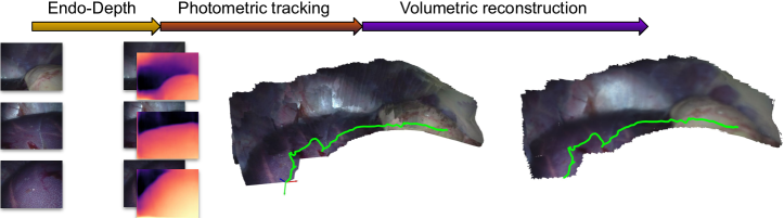
Figure 2: Endo-Depth-and-Motion overview. First, monocular depth is predicted with Endo-Depth. The camera motion (green line) is then estimated using the photometric residuals. Finally, the full scene is reconstructed by volumetric fusion.

Deep convolutional networks were first proposed for depth estimation in [12, 13]. These first models were trained in a supervised manner using depth sensors, and were improved in following works using deeper networks and several architectural contributions [14, 15, 16, 11]. Self-supervised approaches were proposed later, mainly based on multi-view photometric consistency. [17] proposed self-supervision using stereo, and [18] generalized it to monocular views (ego-motion being predicted by another network). Both have been improved in many recent works, e.g., [19, 20]. Self-supervised depth learning is relevant for in-body monocular reconstructions, as it does not require additional sensors, sophisticated renderings [21, 22] or domain transfer [23]. In medical contexts, supervised depth learning has been addressed in [24, 25, 26], self-supervised using stereo in [27] and self-supervised using sparse monocular depth in [28]. [29] is the first that fuses the monocular depths from a supervised network using ElasticFusion [30]. Differently from them, in Endo-Depth we use the state-of-the-art network of [20] with the following advantages: 1) the training is self-supervised from monocular endoscopes, stereo ones, or from both, 2) our experiments show that self-supervised training removes the effect of the domain shift from synthetic data, 3) its dense photometric loss uses the information of the whole image, and 4) several details (e.g, minimum reprojection loss from a set of images) make the loss sufficiently robust to endoscopic image challenges.

Depth and motion can be estimated using only multi-view constraints, either dense [31] or sparse [2]. The literature on these methods is huge, but they are limited on in-body images by drastic illumination changes, weak texture, deformations, tool insertions, fluids and sometimes small camera motions. All of this poses challenges in determining the correspondences and the geometry, that can be alleviated starting from single-view dense depth as we do in Endo-Depth-and-Motion. Convolutional networks are indeed demonstrating a huge potential to replace several parts of SfM/SLAM pipelines [32]. [33, 34] are early works combining single-view depth with multi-view approaches for mapping and tracking respectively. [35] proposed a convolutional model for camera tracking and incremental mapping, in this case tightly integrating multi-view optimization within the network. [5] uses variational auto-encoders for single-view depth and optimizes the depth prediction jointly with the camera poses. The combination we propose is photometric odometry, using the self-supervised Endo-Depth prediction as a pseudo-RGBD keyframe.

The interest for applying SfM/SLAM in intracorporeal sequences has risen following the advances of the field, but encounters the challenges mentioned before. Early monocular approaches were based on the Extended Kalman Filter [36, 37]; and more recent ones on non-linear optimization for tracking and mapping [6] and map densification using variational approaches [38] or multi-view stereo [39]. These methods were strongly based on the rigidity assumption. MIS-SLAM [40, 41] was the first bringing deformable SLAM to intracorporeal images. It uses a canonical shape, as DynamicFusion [42], integrating stereo observations in a Truncated Signed Distance Function (TSDF) [43] with a deformation model. It uses the rigid tracking of ORB-SLAM2 [2] to estimate the camera pose between keyframes. DefSLAM [44] was the first monocular SLAM fully addressing deformations in monocular endoscopies. SD-DefSLAM [45] improves over it incorporating an illumination-invariant Lukas-Kanade tracker, relocalization and tool segmentation. Both of them use at their core an isometric NRSfM (IsoNRSfM) [10] over a sliding window and a robust deformation tracking inspired in [46]. Although IsoNRSfM models intracorporeal deformations, it assumes that the scene is a continuous surface, which does not hold for many in-body scenes. In addition, even in [45], feature correspondence keeps being a challenge. As another drawback, deformable tracking is computationally demanding. Compared to them, our Endo-Depth can be a fair substitute of IsoNRSfM for deformable SLAM. And, under the assumption of slow deformations, our high-keyframe-rate odometry allows Endo-Depth-and-Motion to achieve long tracks in both rigid and deformable in-body sequences.

III Overview

Fig. 2 shows an overview of Endo-Depth-and-Motion. First, pixel-wise depth is predicted on a set of keyframes of the endoscopic monocular video using a deep neural network. This part is described in Section IV. The motion of each frame with respect to the closest keyframe is estimated by minimizing the photometric error, robustified using image pyramids and robust error functions (see Section V for the details). Finally, the depth maps of the keyframes are fused in a TSDF-based volumetric representation, as explained in Section VI. A demonstrative video showing sample results is available as supplementary material.

IV Endo-Depth

We use the Monodepth2 network architecture and training procedures [20], which are the state of the art for self-supervised depth learning. Monodepth2 follows a U-Net encoder-decoder architecture with a ResNet18 encoder, and models the mapping function $f:\mathbb{R}^{w\times h\times 3}\rightarrow\mathbb{R}^{w\times h}$ between an image $I$ of size $w\times h$ and its depth map $D=f(I;\boldsymbol{\theta})$. Fig. 3 shows several examples of predicted depth maps. The network parameters $\boldsymbol{\theta}$ are learned in a self-supervised manner minimizing a total loss $\pazocal{L}=\pazocal{L}_{p}+\lambda\pazocal{L}_{s}$, formed by the weighted sum of a photometric loss $\pazocal{L}_{p}$ and a smoothing loss $\pazocal{L}_{s}$. This last one regularizes the surface while preserving discontinuities at the edges (see details in [20]).

The photometric loss $\pazocal{L}_{p}$ sums over each pixel $\boldsymbol{p}\in\Omega_{t}$ in a target image $I_{t}$ the minimum value of an appearance residual with a pixel $\boldsymbol{p}\in\Omega_{t^{\prime}\rightarrow t}$ in images $I_{t^{\prime}\rightarrow t}$ that are warped from a small set of source images $\pazocal{S}=\{I_{1},\ldots,I_{t^{\prime}},\ldots\}$. The network can be trained using stereo pairs –the target and source images are the stereo ones–, monocular views –the source images are the images before and after the target one–, or both. Specifically, the loss is a function of the photometric reprojection error and the Structural Similarity Index Measure (SSIM) [47]

$${\pazocal{L}_{p}=\sum_{\boldsymbol{p}\in\Omega_{t}}\min_{\pazocal{S}}\left(\alpha\lVert I_{t}\left[\boldsymbol{p}\right]-I_{t^{\prime}\rightarrow t}\left[\boldsymbol{p}\right]\rVert_{1}+\right.}\\ {\left.+\left(1-\text{SSIM}\left(I_{t},I_{t^{\prime}\rightarrow t},\boldsymbol{p}\right)\right)\right)~{},}$$ (1)

where $\left[\cdot\right]$ is the sampling operator and $\alpha$ weights the two addends. The color values of $\boldsymbol{p}\in\Omega_{t^{\prime}\rightarrow t}$ are taken from the corresponding pixels $\boldsymbol{p}^{\prime}\in\Omega_{t^{\prime}}$, so that $I_{t^{\prime}\rightarrow t}\left[\boldsymbol{p}\right]=I_{t^{\prime}}\left[\boldsymbol{p}^{\prime}\right]$. The warping function is

$${\boldsymbol{p}^{\prime}=\pi\left(\mathbf{R}_{t^{\prime}t}\pi^{-1}\left(\boldsymbol{p},D_{t}\left[\boldsymbol{p}\right]\right)+\mathbf{t}_{t^{\prime}t}\right)}$$ (2)

where $\pi:\mathbb{R}^{3}\rightarrow\Omega$ and $\pi^{-1}:\Omega\times\mathbb{R}\rightarrow\mathbb{R}^{3}$ are respectively the projection and back-projection functions. $\mathbf{T}_{t^{\prime}t}=\big{(}\begin{smallmatrix}\mathbf{R}_{t^{\prime}t}&\mathbf{t}_{t^{\prime}t}\\ \mathbf{0}&1\end{smallmatrix}\big{)}\in\mathrm{SE}(3)$, with $\mathbf{R}_{t^{\prime}t}\in\mathrm{SO}(3)$ and $\mathbf{t}_{t^{\prime}t}\in\mathbb{R}^{3}$, is the transformation matrix that converts points from the target reference frame of $I_{t}$ to the source frame of $I_{t^{\prime}}$. Such transformation is pre-calibrated when training with a stereo pair and learned by another deep network when training with two monocular views.

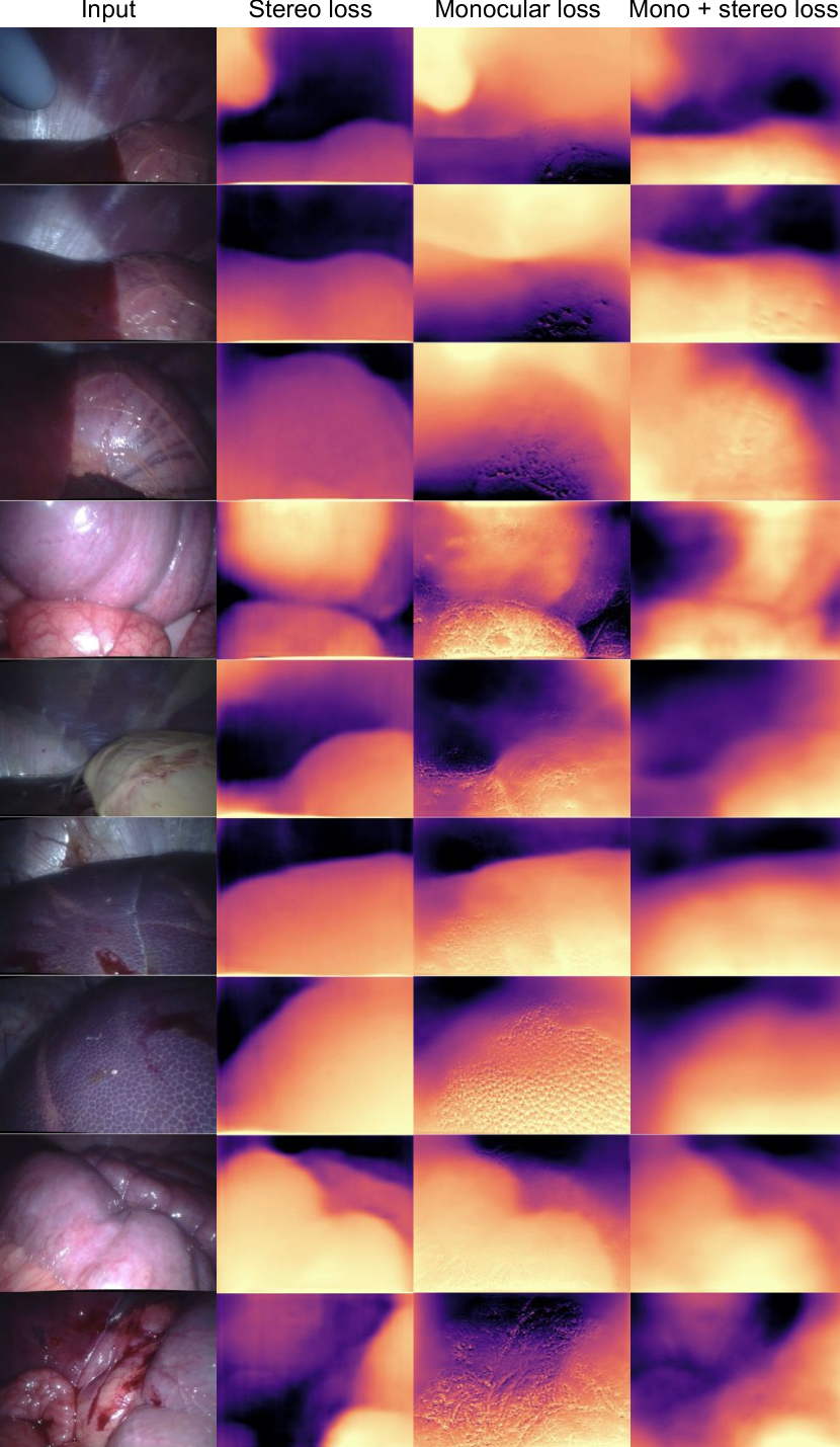
Figure 3: Endo-Depth predictions on sample images of the Hamlyn dataset, trained with different losses.

V Photometric Tracking

We use a keyframe-based photometric approach for tracking the camera pose, that estimates a relative transformation matrix $\mathbf{T}_{ck}\in\mathrm{SE}(3)$ between a target keyframe $I_{k}$ and the current source frame $I_{c}$. Given the dense depth map for the last keyframe $D_{k}=f(I_{k};\boldsymbol{\theta})$, predicted using Endo-Depth (Section IV), we optimize $\mathbf{T}_{ck}$ so that corresponding pixels have minimum color difference. We formulate it as a non-linear least-squares in a Lucas-Kanade style, minimizing the photometric error. To improve the range of convergence, known to be a challenge in photometric methods, we use a coarse-to-fine pyramidal optimization.

Our approach is similar to DTAM [31]. First, we optimize only the camera rotation using the lowest level of the the pyramid. This gives us resilience under motion blur and helps convergence, even when the motion is not a pure rotation. For every scale after the coarser one, we optimize the full six-degrees-of-freedom camera pose. We parametrize local motion updates by using Lie algebras as $\boldsymbol{\psi}\in\mathfrak{se}(3)$. The final cost function is the forward-compositional photometric cost between corresponding pixels in the keyframe $\boldsymbol{p}\in\Omega_{k}$ and in the warped frame $\boldsymbol{p}\in\Omega_{c\rightarrow k}$

$${\\ \hat{\boldsymbol{\psi}}=\operatorname*{arg\,min}_{\boldsymbol{\psi}}\sum_{\boldsymbol{p}\in\Omega_{k}}\min\left(\lVert I_{k}\left[\boldsymbol{p}\right]-I_{c\rightarrow k}\left[\boldsymbol{p}\right]\rVert_{2},\gamma\right)}$$ (3)

where the color value of $\boldsymbol{p}\in\Omega_{c\rightarrow k}$ is taken from its correspondences $\boldsymbol{p}^{\prime}\in\Omega_{c}$ using unprojection and projection as in Equation 2. The frame-to-keyframe motion $\mathbf{T}_{ck}$ is the composition of a global transformation $\mathbf{T}_{ck}^{0}$ and the exponential mapping of the local updates in the Lie algebra $\mathbf{T}_{ck}=\mathrm{exp}_{\mathrm{SE(3)}}(\boldsymbol{\psi})\mathbf{T}_{ck}^{0}$. We use Gauss-Newton, which converges in a few steps. Our tracking does not model occlusions nor illumination changes, as both have a small effect in our narrow baseline setup. In any case, to mitigate the effect of outliers, we saturate the L2-norm of the residuals with a threshold $\gamma$ determined experimentally.

VI Volumetric Reconstruction

In this final stage of our pipeline, we fuse the registered pseudo-RGBD keyframes obtained from Endo-Depth after tracking into an implicit surface representation. Specifically, we use a TSDF [43]. The scene is first divided into voxels and, for each of them it is stored a cumulative signed distance function $d:\mathbb{R}^{3}\rightarrow\mathbb{R}$ that represents the distance to the closest surface (which it is truncated at a certain depth value). The TSDF can be updated in a straightforward manner, using sequential averaging for every voxel and the predicted depth for every pixel $\boldsymbol{p}\in\Omega_{k}$ in every keyframe $k$. The surface can be efficiently recovered from such implicit representation using, for instance, the Marching Cubes algorithm [48]. In our experiments, we use the implementation in Open3D [49].

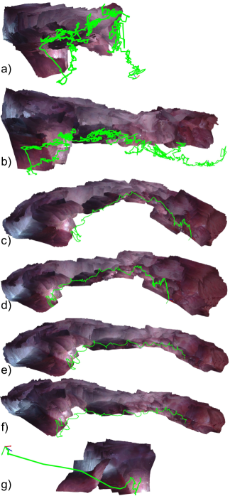
Figure 4: Trajectory and reconstructions before fusion in Hamlyn video #22 for 7 tracking alternatives: a) point-to-point ICP [50], b) point-to-plane ICP [51], c) photometric [52], d) photometric plus geometric [53] and ours with keyframe creation ratio e) $0.5$, f) $0.2$ and g) $0.1$.

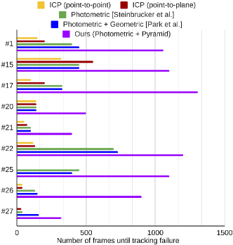
Figure 5: Frames until failure for 5 tracking alternatives (ICP point-to-point [50], ICP point-to-plane [51], photometric [52], hybrid photometric and geometric [53] and ours) in 9 Hamlyn videos (same as the maps in Fig. 1, 2 and 4).

VII Experimental Results

We used the Hamlyn dataset [54, 55, 56, 57], that contains challenging sequences imaging intracorporeal scenes with weak textures, deformations, reflections, surgical tools and occlusions. Specifically, we chose 21 videos with diverse image resolution and calibration parameters.

VII-A Endo-Depth

Fig. 3 shows Endo-Depth predictions for several sample images of the Hamlyn dataset. To obtain quantitative results, we generated ground truth depth from stereo, specifically using Libelas (Library for Efficient Large-Scale Stereo Matching [58]). It must be remarked that Libelas is sufficiently good but not perfect: it leaves blank areas for pixels at image borders and sometimes within the image. This ground truth is made available to be used as benchmark and can be found in our project page.

We defined the configuration for self-supervised training after an extensive ablation study. First, we set the input size to half of the original images. In this manner we filter details like veins, small folds or specular reflections that cause color changes unrelated to depth. Also, using reflection padding (instead of the more usual zero padding) in the decoder demonstrated a better performance both qualitatively and quantitatively. Many works [20, 59, 60, 61] used an encoder pretrained for ImageNet classification [62], achieving smaller errors compared to training from scratch. For Monodepth2, pretraining is also benefitial when evaluated in KITTI [63], and we have seen the same effect for Endo-Depth evaluated in Hamlyn. Summing up, all our models were pre-trained in ImageNet, and trained in Hamlyn halving the resolution of the input images and with reflection padding. With stereo and monocular-stereo data, the best performance was reached after 2 epochs. When training only with monocular images, 9 epochs were necessary.

We do 21-fold cross validation for each training modality in Tables I and II. Each of the 21 models is tested on one Hamlyn video and trained on the rest. To address the varying camera intrinsics in the Hamlyn data, we grouped together videos that have similar resolution and intrinsics and trained Endo-Depth sequentially in each of them. For the training splits we removed occluded or useless frames, and for the test ones, also those frames with low-quality ground truth. We report the standard metrics for depth networks [12]. As monocular depth is affected of scale drift, in particular if trained with monocular sequences, we align the scales of the predicted depth $D_{i}$ and the ground truth depth $D_{i}^{GT}$ using a per-image scale factor $s_{i}$ computed, as it is standard in the literature [12], as $s_{i}=\nicefrac{{\text{median}(D_{i}^{GT})}}{{\text{median}(D_{i})}}$. We show in the last column of Table I that the stereo loss achieves the best performance in most of the sequences. This is expected, since the illumination does not change nor the scene deforms between the images of a stereo pair. On the other side, the monocular loss is affected by these two factors, in addition to having to learn the relative camera motion.

Table II shows Endo-Depth results without depth scaling, as stereo self-supervision observes such scale. We consider this a more realistic setup and a more relevant metric for applications. Notice that the differences with per-image scaling are small (less than $1$ cm RMSE in average). This demonstrates that Endo-Depth trained with monocular-stereo or stereo losses learns a stable global scale for the reconstruction, which is a key aspect to obtain small trajectory drift in the experiments of Section VII-B.

		Sequence
	Loss	1	4	5	6	8	11	12	14	15	16	17	18	19	20	21	22	23	24	25	26	27	#-Best
	Mono	0.260	0.059	0.064	0.152	0.132	0.112	0.089	0.162	0.109	0.100	0.232	0.308	0.296	0.115	0.123	0.230	0.252	0.241	0.146	0.157	0.178	0/21
	Stereo	0.091	0.038	0.047	0.080	0.120	0.092	0.040	0.136	0.070	0.072	0.195	0.230	0.184	0.109	0.108	0.158	0.166	0.183	0.141	0.131	0.128	18/21
Abs Rel	Mono + Stereo	0.193	0.040	0.073	0.432	0.114	0.079	0.109	0.163	0.088	0.095	0.222	0.232	0.272	0.095	0.137	0.211	0.215	0.201	0.171	0.168	0.152	3/21
	Mono	19.775	0.269	0.335	6.461	2.738	1.491	1.629	3.859	0.796	1.102	6.175	10.802	12.437	1.093	1.681	5.689	9.159	6.260	2.318	2.874	4.247	1/21
	Stereo	1.429	0.160	0.186	1.057	1.951	1.332	0.651	2.855	0.425	0.751	5.344	6.994	4.379	1.084	1.581	3.147	4.954	3.664	2.471	2.407	2.371	16/21
Sq Rel	Mono + Stereo	9.251	0.193	0.458	56.218	1.906	0.931	1.442	3.861	0.643	1.111	5.676	6.415	9.699	0.723	2.344	4.772	7.936	4.136	3.224	3.072	3.204	4/21
	Mono	30.617	3.405	3.859	23.488	14.301	9.978	10.232	14.142	5.279	6.796	19.540	28.302	24.495	7.057	9.272	18.805	21.619	18.321	10.754	12.872	15.517	1/21
	Stereo	9.792	2.385	2.855	10.653	11.296	9.156	6.156	11.833	3.537	5.258	17.793	21.772	15.723	6.816	8.760	13.848	16.003	14.522	11.022	11.862	11.072	18/21
RMSE	Mono + Stereo	21.042	2.572	4.472	55.892	11.729	7.790	10.160	13.068	4.798	6.648	18.868	21.984	22.274	5.735	10.657	17.145	19.263	15.523	12.489	13.506	12.570	2/21
	Mono	0.287	0.075	0.083	0.187	0.188	0.159	0.126	0.217	0.156	0.130	0.272	0.361	0.320	0.145	0.152	0.271	0.284	0.294	0.186	0.197	0.213	0/21
	Stereo	0.114	0.052	0.061	0.099	0.154	0.126	0.070	0.183	0.099	0.099	0.239	0.279	0.230	0.138	0.141	0.199	0.206	0.226	0.179	0.169	0.161	17/21
RMSElog	Mono + Stereo	0.230	0.056	0.093	0.400	0.153	0.112	0.146	0.212	0.144	0.123	0.262	0.278	0.310	0.118	0.173	0.251	0.254	0.245	0.213	0.208	0.185	4/21
	Mono	0.747	0.989	0.995	0.810	0.810	0.864	0.921	0.767	0.887	0.915	0.586	0.453	0.557	0.865	0.860	0.567	0.647	0.595	0.804	0.776	0.735	1/21
	Stereo	0.928	0.989	0.999	0.952	0.866	0.941	0.984	0.808	0.952	0.948	0.717	0.628	0.727	0.876	0.885	0.761	0.810	0.711	0.832	0.837	0.842	19/21
$\delta<1.25^{1}$	Mono + Stereo	0.780	0.987	0.968	0.610	0.857	0.962	0.888	0.776	0.908	0.917	0.630	0.574	0.583	0.930	0.838	0.619	0.754	0.642	0.768	0.738	0.791	2/21
	Mono	0.890	1.000	1.000	0.963	0.955	0.989	0.984	0.924	0.975	0.988	0.884	0.764	0.823	0.993	0.985	0.891	0.856	0.872	0.962	0.956	0.942	4/21
	Stereo	0.989	0.999	1.000	0.999	0.980	0.989	0.991	0.950	0.992	0.990	0.915	0.870	0.921	0.990	0.980	0.955	0.923	0.930	0.960	0.967	0.972	14/21
$\delta<1.25^{2}$	Mono + Stereo	0.946	0.999	0.999	0.861	0.980	0.993	0.993	0.936	0.971	0.985	0.893	0.873	0.842	0.999	0.962	0.910	0.881	0.922	0.944	0.952	0.959	5/21
	Mono	0.940	1.000	1.000	0.989	0.989	0.994	0.995	0.978	0.995	0.997	0.980	0.937	0.941	1.000	0.998	0.986	0.940	0.959	0.995	0.993	0.990	5/21
	Stereo	0.998	1.000	1.000	1.000	0.996	0.995	0.995	0.986	0.999	0.998	0.977	0.967	0.978	0.999	0.998	0.991	0.975	0.992	0.993	0.994	0.995	13/21
$\delta<1.25^{3}$	Mono + Stereo	0.974	1.000	1.000	0.898	0.997	0.996	0.996	0.977	0.993	0.999	0.985	0.983	0.948	1.000	0.996	0.990	0.945	0.989	0.985	0.994	0.991	10/21

TABLE I: Endo-Depth results in Hamlyn with per-image scaling. $\text{Abs}_{\text{rel}}$ and RMSE in [mm], $\text{RMSE}_{\text{log}}$ in [log mm]. We compare three losses: pure monocular (Mono), stereo (Stereo) and a combination of both (Mono + Stereo). 1 column: metrics used for evaluation. 2 column: losses used during training. Last column: number of times a method is the best for a given metric. Rest of the columns: results for the Hamlyn sequences.

		Sequence
	Loss	1	4	5	6	8	11	12	14	15	16	17	18	19	20	21	22	23	24	25	26	27	#-Best
	Stereo	0.573	0.070	0.062	0.342	0.642	0.168	0.203	0.209	0.105	0.174	0.222	0.255	0.236	0.192	0.128	0.198	0.182	0.365	0.158	0.156	0.224	18/21
Abs Rel	Mono + Stereo	0.312	0.070	0.079	0.571	0.754	0.086	0.295	0.514	0.719	0.396	0.343	0.262	0.379	0.279	0.208	0.267	0.273	0.447	0.420	0.347	0.189	4/21
	Stereo	29.813	0.337	0.262	19.045	32.455	2.724	3.323	3.916	0.576	2.375	8.182	8.428	6.662	3.429	1.713	5.538	5.478	13.119	2.932	2.919	5.067	17/21
Sq Rel	Mono + Stereo	18.939	0.392	0.530	83.030	41.415	1.057	6.415	13.947	15.758	9.142	12.983	7.743	12.800	4.599	4.640	8.038	7.842	17.415	13.131	9.939	3.928	4/21
	Stereo	44.538	3.605	3.570	29.569	38.724	12.649	15.521	13.724	4.152	9.971	20.678	24.102	18.435	11.130	9.605	16.963	16.622	24.723	11.799	13.138	17.851	18/21
RMSE	Mono + Stereo	27.863	3.690	4.799	65.822	44.831	8.237	20.921	23.659	20.948	19.805	26.075	24.948	30.643	13.813	14.505	20.749	21.462	28.698	24.522	22.421	15.660	3/21
	Stereo	0.452	0.081	0.075	0.273	0.484	0.183	0.245	0.232	0.130	0.181	0.269	0.304	0.271	0.200	0.155	0.233	0.216	0.352	0.195	0.195	0.294	18/21
RMSElog	Mono + Stereo	0.306	0.083	0.100	0.472	0.547	0.120	0.388	0.431	0.546	0.347	0.353	0.311	0.550	0.263	0.226	0.292	0.289	0.407	0.385	0.334	0.242	3/21
	Stereo	0.158	0.990	0.999	0.632	0.199	0.800	0.488	0.696	0.941	0.837	0.763	0.555	0.663	0.718	0.852	0.733	0.815	0.524	0.772	0.774	0.467	18/21
$\delta<1.25^{1}$	Mono + Stereo	0.606	0.984	0.961	0.455	0.153	0.956	0.160	0.299	0.071	0.276	0.569	0.486	0.182	0.470	0.700	0.613	0.529	0.413	0.401	0.438	0.609	3/21
	Stereo	0.492	1.000	1.000	0.787	0.545	0.983	0.983	0.935	0.988	0.972	0.867	0.840	0.867	0.940	0.989	0.902	0.917	0.769	0.956	0.960	0.828	18/21
$\delta<1.25^{2}$	Mono + Stereo	0.838	1.000	0.999	0.765	0.381	0.992	0.752	0.595	0.220	0.810	0.794	0.822	0.425	0.938	0.927	0.839	0.889	0.698	0.671	0.802	0.911	4/21
	Stereo	0.894	1.000	1.000	0.886	0.792	0.994	0.990	0.980	0.997	0.996	0.943	0.961	0.961	0.996	0.998	0.975	0.969	0.908	0.990	0.993	0.975	16/21
$\delta<1.25^{3}$	Mono + Stereo	0.958	1.000	1.000	0.872	0.724	0.995	0.971	0.830	0.853	0.973	0.893	0.982	0.742	0.998	0.983	0.962	0.958	0.874	0.926	0.956	0.993	7/21

TABLE II: Endo-Depth results in Hamlyn without scaling. $\text{Abs}_{\text{rel}}$ and RMSE in [mm], $\text{RMSE}_{\text{log}}$ in [log mm]. We compare two losses that predict real scale: (Stereo) and its combination with monocular self-supervision (Mono + Stereo). 1 column: metrics used for evaluation. 2 column: losses used during training. Last column: number of times a method is the best for a given metric. Rest of the columns: results for the Hamlyn sequences.

		Sequence
	Method	1	4	19	20
	LapDepth [11]	0.504	0.432	1.234	0.847
	IsoNRSfM [10]	0.097	0.048	0.062	0.064
	ours Mono	0.293	0.054	0.235	0.134
	ours Stereo	0.083	0.024	0.169	0.120
Abs Rel	ours Mono + Stereo	0.213	0.023	0.284	0.087
	LapDepth [11]	29.132	12.182	75.260	39.121
	IsoNRSfM [10]	2.563	0.185	0.769	0.578
	ours Mono	26.497	0.204	7.432	1.487
	ours Stereo	1.379	0.051	5.275	1.212
Sq Rel	ours Mono + Stereo	11.822	0.052	11.768	0.603
	LapDepth [11]	20.710	11.742	26.742	15.599
	IsoNRSfM [10]	19.815	2.698	6.478	6.420
	ours Mono	34.382	2.937	18.640	8.354
	ours Stereo	9.361	1.432	16.213	7.491
RMSE	ours Mono + Stereo	23.553	1.428	24.026	5.401
	LapDepth [11]	0.417	0.408	0.703	0.575
	IsoNRSfM [10]	0.122	0.063	0.095	0.084
	ours Mono	0.310	0.068	0.264	0.168
	ours Stereo	0.109	0.032	0.228	0.147
RMSElog	ours Mono + Stereo	0.251	0.032	0.328	0.108
	LapDepth [11]	0.692	0.668	0.493	0.649
	IsoNRSfM [10]	0.930	0.997	0.960	0.988
	ours Mono	0.741	0.997	0.595	0.799
	ours Stereo	0.926	1.000	0.796	0.845
$\delta<1.25^{1}$	ours Mono + Stereo	0.762	1.000	0.689	0.959
	LapDepth [11]	0.917	0.925	0.762	0.875
	IsoNRSfM [10]	0.998	1.000	0.997	1.000
	ours Mono	0.881	1.000	0.921	0.988
	ours Stereo	0.988	1.000	0.910	0.995
$\delta<1.25^{2}$	ours Mono + Stereo	0.931	1.000	0.832	0.999
	LapDepth [11]	0.964	0.967	0.872	0.930
	IsoNRSfM [10]	0.999	1.000	1.000	1.000
	ours Mono	0.928	1.000	0.988	0.999
	ours Stereo	0.998	1.000	0.964	1.000
$\delta<1.25^{3}$	ours Mono + Stereo	0.965	1.000	0.909	1.000

TABLE III: Comparison against baselines [10] and [11] in Hamlyn. $\text{Abs}_{\text{rel}}$ and RMSE in [mm], $\text{RMSE}_{\text{log}}$ in [log mm]. Best results are boldfaced, second best are underlined.

Table III shows the comparison between Endo-Depth and the baselines LapDepth [11] and IsoNRSfM [10]. LapDepth is a state-of-the-art supervised depth network, that we trained in the synthetic dataset of [26], containing $16K$ images, using the authors’ default configuration. IsoNRSfM is a multi-view method for which we chose the state-of-the-art implementation of [45]. However, we re-ran IsoNRSfM and obtained even better results than [45]. We use the per-image scaling as in [45], $s_{i}^{\prime}=\text{median}\left(\nicefrac{{D_{i}^{GT}}}{{D_{i}}}\right)$. Although it is slightly different from the one in Table I, we prefer to keep the metrics strictly as they were defined in each of our references. Notice that Table III reports IsoNRSfM results only in keyframes and only for the sparse point cloud, while Endo-Depth and LapDepth report dense ones. Note also that we are able to run Endo-Depth in a larger set of Hamlyn sequences than IsoNRSfM (21 of them, see Tables I and II). We compare the three methods in four different sequences. In video #1 the camera explores the abdominal wall from a distant point causing a small stereo parallax, hindering the evaluation. In video #4, the camera is static and captures a beating heart. Video #19, shows challenging organ deformations with low texture and tool intrusion. Lastly, video #20, images a deforming intestine. Such deformations and tools intrusions challenge the assumptions made by the monocular self-supervision, but our results are still competitive. Endo-Depth has three main advantages for deformable mapping versus IsoNRSfM. First, we recover the dense depth of the entire image without the limitation of finding multi-view correspondences. Second, as shown in Fig. 3, we can cope with discontinuities. And finally, we can do it with a single-shot, allowing us to initialize depth without a sliding window of images. This last point is crucial in intracorporeal sequences where the lack of texture compromises the matching. Finally, observe how LapDepth performs significantly worse than Endo-Depth even if it was trained in supervised data. The reason is the domain shift between the synthetic and real images, which is our motivation to use self-supervised training.

The computation time of Endo-Depth for one test image is $\sim$$15$ ms in a Nvidia RTX 2080Ti GPU and $\sim$$55$ ms in a AMD Ryzen 9 3900X CPU. IsoNRSfM, for the same image, including warps and alignment, takes $\sim 500$ ms in a Intel i7-7700K CPU. For a better visualization of Endo-Depth results, the reader is referred to our supplementary videos, that contain depth predictions for five Hamlyn test videos with our best training setup (stereo loss), together with their backprojected 3D point clouds and the ground truth.

VII-B Camera Tracking

Fig. 4 and Fig. 5 show qualitative and quantitative results of our photometric tracking versus other alternatives. Specifically, we compare it against the Open3D [49] implementations of ICP (using point-to-point and point-to-plane distances) and pose tracking using photometric and hybrid photometric and geometric residuals (at optimal keyframe creation ratios). We also show different keyframe creation ratios in Fig. 4, being the higher ones the more convenient due to fast camera dynamics in these sequences. The computation time per frame of our Python implementation is around $300$ ms in our GPU (Nvidia RTX 2080Ti) and $700$ ms in CPU (AMD Ryzen 9 3900X).

VII-C Volumetric Fusion

Fig. 6 shows sample 3D reconstructions after fusing the predicted depth maps in a TSDF representation in 7 Hamlyn videos, chosen among those with larger camera translation. Although the ground truth for the scene and camera trajectory is not available, the accuracy of the reconstruction can be qualitatively assessed in the figure. Notice that we present a higher number of reconstructions and of larger extent than other approaches in the literature (e.g., [41, 44, 45]), which again highlights the potential of depth networks, photometric pseudo-RGBD tracking and volumetric fusion for reconstruction and motion estimation in monocular endoscopies. The Python implementation runs within reasonable time limits, the volumetric fusion of a $1200$-frames reconstruction taking $\sim$$7$ s in our CPU (AMD Ryzen 9 3900X).

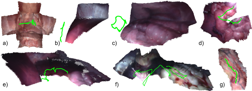
Figure 6: Maps after volumetric fusion of several Hamlyn videos: a) #1, b) #15, c) #17. d) #20, e) #21, f) #25 and g) #27.

VIII Conclusions and Future Work

In this paper we have presented Endo-Depth-and-Motion, in which we train and evaluate thoroughly state-of-the-art self-supervised depth learning in endoscopic videos, implement a robust photometric odometry and integrate their outputs with a volumetric fusion approach. Several conclusions can be extracted from our evaluation. Firstly, our self-supervised depth network Endo-Depth, trained in the Hamlyn sequences, has a competitive performance even when compared against well-established multi-view baselines such as IsoNRSfM and supervised networks as LapDepth. This suggests that relevant future work could come out from the replacement of IsoNRSfM templates and supervised depth learning in SfM/SLAM pipelines for endoscopies. Importantly, such performance does not degrade when evaluated without per-image scaling, showing that the global scale of the scene can be effectively learned using stereo losses. Secondly, we implement a photometric dense tracking for estimating the camera motion with respect a pseudo-RGBD keyframe. Finally, we fuse the predicted depth maps of the registered keyframes using a TSDF representation, showing again a satisfactory performance. Our main line for future work is including deformation models in our scene representation.

References

- [1] J. L. Schonberger and J.-M. Frahm, “Structure-from-motion revisited,” in IEEE conference on computer vision and pattern recognition, 2016.
- [2] R. Mur-Artal and J. D. Tardós, “ORB-SLAM2: An open-source SLAM system for monocular, stereo, and RGB-D cameras,” IEEE Transactions on Robotics, vol. 33, no. 5, pp. 1255–1262, 2017.
- [3] J. Engel, T. Schöps, and D. Cremers, “LSD-SLAM: Large-scale direct monocular SLAM,” in European conference on computer vision, 2014.
- [4] S. H. Lee and J. Civera, “Loosely-coupled semi-direct monocular SLAM,” IEEE Robotics and Automation Letters, vol. 4, no. 2, pp. 399–406, 2018.
- [5] J. Czarnowski, T. Laidlow, R. Clark, and A. J. Davison, “DeepFactors: Real-time probabilistic dense monocular SLAM,” IEEE Robotics and Automation Letters, vol. 5, no. 2, pp. 721–728, 2020.
- [6] N. Mahmoud, Ó. G. Grasa, S. A. Nicolau, C. Doignon, L. Soler, J. Marescaux, and J. Montiel, “On-patient see-through augmented reality based on visual SLAM,” International journal of computer assisted radiology and surgery, vol. 12, no. 1, pp. 1–11, 2017.
- [7] J. V. Rijn, J. B. Reitsma, J. Stoker, P. M. Bossuyt, S. J. Van Deventer, and E. Dekker, “Polyp miss rate determined by tandem colonoscopy: a systematic review,” Official journal of the American College of Gastroenterology, vol. 101, no. 2, pp. 343–350, 2006.
- [8] R. Ma, R. Wang, S. Pizer, J. Rosenman, S. K. McGill, and J.-M. Frahm, “Real-time 3D reconstruction of colonoscopic surfaces for determining missing regions,” in International Conference on Medical Image Computing and Computer-Assisted Intervention, 2019.
- [9] G. Fagogenis, M. Mencattelli, Z. Machaidze, B. Rosa, K. Price, F. Wu, V. Weixler, M. Saeed, J. E. Mayer, and P. E. Dupont, “Autonomous robotic intracardiac catheter navigation using haptic vision,” Science robotics, vol. 4, no. 29, 2019.
- [10] S. Parashar, D. Pizarro, and A. Bartoli, “Isometric Non-Rigid Shape-from-Motion with Riemannian Geometry Solved in Linear Time,” IEEE Transactions on Pattern Analysis and Machine Intelligence, vol. 40, no. 10, pp. 2442–2454, 2018.
- [11] M. Song, S. Lim, and W. Kim, “Monocular depth estimation using laplacian pyramid-based depth residuals,” IEEE Transactions on Circuits and Systems for Video Technology, 2021.
- [12] D. Eigen, C. Puhrsch, and R. Fergus, “Depth map prediction from a single image using a multi-scale deep network,” in Proc. of the Conference on Neural Information Processing Systems, 2014.
- [13] D. Eigen and R. Fergus, “Predicting depth, surface normals and semantic labels with a common multi-scale convolutional architecture,” in IEEE international conference on computer vision, 2015.
- [14] I. Laina, C. Rupprecht, V. Belagiannis, F. Tombari, and N. Navab, “Deeper depth prediction with fully convolutional residual networks,” in Fourth international conference on 3D vision, 2016.
- [15] H. Fu, M. Gong, C. Wang, K. Batmanghelich, and D. Tao, “Deep ordinal regression network for monocular depth estimation,” in IEEE Conference on Computer Vision and Pattern Recognition, 2018.
- [16] J. M. Facil, B. Ummenhofer, H. Zhou, L. Montesano, T. Brox, and J. Civera, “CAM-Convs: camera-aware multi-scale convolutions for single-view depth,” in IEEE/CVF Conference on Computer Vision and Pattern Recognition, 2019.
- [17] C. Godard, O. Mac Aodha, and G. J. Brostow, “Unsupervised monocular depth estimation with left-right consistency,” in IEEE Conference on Computer Vision and Pattern Recognition, 2017.
- [18] T. Zhou, M. Brown, N. Snavely, and D. G. Lowe, “Unsupervised learning of depth and ego-motion from video,” in IEEE Conference on Computer Vision and Pattern Recognition, 2017.
- [19] H. Zhan, R. Garg, C. Saroj Weerasekera, K. Li, H. Agarwal, and I. Reid, “Unsupervised learning of monocular depth estimation and visual odometry with deep feature reconstruction,” in IEEE Conference on Computer Vision and Pattern Recognition, 2018.
- [20] C. Godard, O. Mac Aodha, M. Firman, and G. J. Brostow, “Digging into self-supervised monocular depth estimation,” in IEEE/CVF International Conference on Computer Vision, 2019.
- [21] F. Mahmood, R. Chen, S. Sudarsky, D. Yu, and N. J. Durr, “Deep learning with cinematic rendering: fine-tuning deep neural networks using photorealistic medical images,” Physics in Medicine & Biology, vol. 63, no. 18, p. 185012, 2018.
- [22] K. İncetan, I. O. Celik, A. Obeid, G. I. Gokceler, K. B. Ozyoruk, Y. Almalioglu, R. J. Chen, F. Mahmood, H. Gilbert, N. J. Durr et al., “VR-Caps: A Virtual Environment for Capsule Endoscopy,” Medical image analysis, vol. 70, p. 101990, 2021.
- [23] F. Mahmood, R. Chen, and N. J. Durr, “Unsupervised reverse domain adaptation for synthetic medical images via adversarial training,” IEEE transactions on medical imaging, vol. 37, no. 12, pp. 2572–2581, 2018.
- [24] M. Visentini-Scarzanella, T. Sugiura, T. Kaneko, and S. Koto, “Deep monocular 3d reconstruction for assisted navigation in bronchoscopy,” International journal of computer assisted radiology and surgery, vol. 12, no. 7, pp. 1089–1099, 2017.
- [25] M. Shen, Y. Gu, N. Liu, and G.-Z. Yang, “Context-aware depth and pose estimation for bronchoscopic navigation,” IEEE Robotics and Automation Letters, vol. 4, no. 2, pp. 732–739, 2019.
- [26] A. Rau, P. E. Edwards, O. F. Ahmad, P. Riordan, M. Janatka, L. B. Lovat, and D. Stoyanov, “Implicit domain adaptation with conditional generative adversarial networks for depth prediction in endoscopy,” International journal of computer assisted radiology and surgery, vol. 14, no. 7, pp. 1167–1176, 2019.
- [27] K. Xu, Z. Chen, and F. Jia, “Unsupervised binocular depth prediction network for laparoscopic surgery,” Computer Assisted Surgery, vol. 24, no. sup1, pp. 30–35, 2019.
- [28] X. Liu, A. Sinha, M. Ishii, G. D. Hager, A. Reiter, R. H. Taylor, and M. Unberath, “Dense depth estimation in monocular endoscopy with self-supervised learning methods,” IEEE transactions on medical imaging, vol. 39, no. 5, pp. 1438–1447, 2019.
- [29] R. J. Chen, T. L. Bobrow, T. Athey, F. Mahmood, and N. J. Durr, “SLAM endoscopy enhanced by adversarial depth prediction,” KDD Workshop on Applied Data Science for Healthcare, 2019.
- [30] T. Whelan, R. F. Salas-Moreno, B. Glocker, A. J. Davison, and S. Leutenegger, “ElasticFusion: Real-time dense SLAM and light source estimation,” The International Journal of Robotics Research, vol. 35, no. 14, pp. 1697–1716, 2016.
- [31] R. A. Newcombe, S. J. Lovegrove, and A. J. Davison, “DTAM: Dense tracking and mapping in real-time,” in 2011 International Conference on Computer Vision, 2011.
- [32] C. Cadena, L. Carlone, H. Carrillo, Y. Latif, D. Scaramuzza, J. Neira, I. Reid, and J. J. Leonard, “Past, present, and future of simultaneous localization and mapping: Toward the robust-perception age,” IEEE Transactions on robotics, vol. 32, no. 6, pp. 1309–1332, 2016.
- [33] J. M. Fácil, A. Concha, L. Montesano, and J. Civera, “Single-view and multi-view depth fusion,” IEEE Robotics and Automation Letters, vol. 2, no. 4, pp. 1994–2001, 2017.
- [34] K. Tateno, F. Tombari, I. Laina, and N. Navab, “CNN-SLAM: Real-time dense monocular SLAM with learned depth prediction,” in IEEE Conference on Computer Vision and Pattern Recognition, 2017.
- [35] H. Zhou, B. Ummenhofer, and T. Brox, “DeepTAM: Deep tracking and mapping with convolutional neural networks,” International Journal of Computer Vision, vol. 128, no. 3, pp. 756–769, 2020.
- [36] O. G. Grasa, J. Civera, and J. Montiel, “EKF monocular SLAM with relocalization for laparoscopic sequences,” in 2011 IEEE International Conference on Robotics and Automation. IEEE, 2011, pp. 4816–4821.
- [37] O. G. Grasa, E. Bernal, S. Casado, I. Gil, and J. Montiel, “Visual SLAM for handheld monocular endoscope,” IEEE transactions on medical imaging, vol. 33, no. 1, pp. 135–146, 2013.
- [38] N. Mahmoud, T. Collins, A. Hostettler, L. Soler, C. Doignon, and J. M. M. Montiel, “Live tracking and dense reconstruction for handheld monocular endoscopy,” IEEE transactions on medical imaging, vol. 38, no. 1, pp. 79–89, 2018.
- [39] A. Marmol, A. Banach, and T. Peynot, “Dense-ArthroSLAM: Dense intra-articular 3-D reconstruction with robust localization prior for arthroscopy,” IEEE Robotics and Automation Letters, vol. 4, no. 2, pp. 918–925, 2019.
- [40] J. Song, J. Wang, L. Zhao, S. Huang, and G. Dissanayake, “Dynamic reconstruction of deformable soft-tissue with stereo scope in minimal invasive surgery,” IEEE Robotics and Automation Letters, vol. 3, no. 1, pp. 155–162, 2017.
- [41] ——, “MIS-SLAM: Real-time large-scale dense deformable SLAM system in minimal invasive surgery based on heterogeneous computing,” IEEE Robotics and Automation Letters, vol. 3, no. 4, pp. 4068–4075, 2018.
- [42] R. A. Newcombe, D. Fox, and S. M. Seitz, “DynamicFusion: Reconstruction and tracking of non-rigid scenes in real-time,” in IEEE conference on computer vision and pattern recognition, 2015.
- [43] B. Curless and M. Levoy, “A volumetric method for building complex models from range images,” in Proceedings of the 23rd annual conference on Computer graphics and interactive techniques, 1996, pp. 303–312.
- [44] J. Lamarca, S. Parashar, A. Bartoli, and J. M. M. Montiel, “DefSLAM: Tracking and Mapping of Deforming Scenes From Monocular Sequences,” IEEE Transactions on Robotics, vol. 37, no. 1, pp. 291–303, 2021.
- [45] J. J. Gómez Rodríguez, J. Lamarca, J. Morlana, J. D. Tardós, and J. M. Montiel, “SD-DefSLAM: Semi-Direct Monocular SLAM for Deformable and Intracorporeal Scenes,” in IEEE International Conference on Robotics and Automation, 2021.
- [46] J. Lamarca and J. M. M. Montiel, “Camera tracking for SLAM in deformable maps,” in Proceedings of the European Conference on Computer Vision (ECCV) Workshops, 2018.
- [47] Z. Wang, A. C. Bovik, H. R. Sheikh, and E. P. Simoncelli, “Image quality assessment: from error visibility to structural similarity,” IEEE transactions on image processing, vol. 13, no. 4, pp. 600–612, 2004.
- [48] W. E. Lorensen and H. E. Cline, “Marching cubes: A high resolution 3D surface construction algorithm,” ACM siggraph computer graphics, vol. 21, no. 4, pp. 163–169, 1987.
- [49] Q.-Y. Zhou, J. Park, and V. Koltun, “Open3D: A modern library for 3D data processing,” arXiv:1801.09847, 2018.
- [50] P. J. Besl and N. D. McKay, “Method for registration of 3-D shapes,” in Sensor fusion IV: control paradigms and data structures, vol. 1611. International Society for Optics and Photonics, 1992, pp. 586–606.
- [51] Y. Chen and G. Medioni, “Object modelling by registration of multiple range images,” Image and vision computing, vol. 10, no. 3, pp. 145–155, 1992.
- [52] F. Steinbrücker, J. Sturm, and D. Cremers, “Real-time visual odometry from dense RGB-D images,” in 2011 IEEE international conference on computer vision workshops (ICCV Workshops), 2011.
- [53] J. Park, Q.-Y. Zhou, and V. Koltun, “Colored point cloud registration revisited,” in IEEE international conference on computer vision, 2017.
- [54] P. Mountney, D. Stoyanov, and G.-Z. Yang, “Three-dimensional tissue deformation recovery and tracking,” IEEE Signal Processing Magazine, vol. 27, no. 4, pp. 14–24, 2010.
- [55] D. Stoyanov, G. P. Mylonas, F. Deligianni, A. Darzi, and G. Z. Yang, “Soft-tissue motion tracking and structure estimation for robotic assisted mis procedures,” in International Conference on Medical Image Computing and Computer-Assisted Intervention, 2005, pp. 139–146.
- [56] D. Stoyanov, M. V. Scarzanella, P. Pratt, and G.-Z. Yang, “Real-time stereo reconstruction in robotically assisted minimally invasive surgery,” in International Conference on Medical Image Computing and Computer-Assisted Intervention, 2010.
- [57] P. Pratt, D. Stoyanov, M. Visentini-Scarzanella, and G.-Z. Yang, “Dynamic guidance for robotic surgery using image-constrained biomechanical models,” in International Conference on Medical Image Computing and Computer-Assisted Intervention, 2010, pp. 77–85.
- [58] A. Geiger, M. Roser, and R. Urtasun, “Efficient large-scale stereo matching,” in Asian conference on computer vision, 2010, pp. 25–38.
- [59] R. Girshick, J. Donahue, T. Darrell, and J. Malik, “Rich feature hierarchies for accurate object detection and semantic segmentation,” in IEEE conference on computer vision and pattern recognition, 2014.
- [60] Y. Kuznietsov, J. Stuckler, and B. Leibe, “Semi-supervised deep learning for monocular depth map prediction,” in IEEE conference on computer vision and pattern recognition, 2017.
- [61] X. Guo, H. Li, S. Yi, J. Ren, and X. Wang, “Learning monocular depth by distilling cross-domain stereo networks,” in European Conference on Computer Vision, 2018.
- [62] Olga Russakovsky et al., “ImageNet Large Scale Visual Recognition Challenge,” International journal of computer vision, vol. 115, no. 3, pp. 211–252, 2015.
- [63] A. Geiger, P. Lenz, C. Stiller, and R. Urtasun, “Vision meets robotics: The KITTI dataset,” The International Journal of Robotics Research, vol. 32, no. 11, pp. 1231–1237, 2013.