On a Standard Method for Measuring the
Natural Rate of Interest

Abstract

I show that Holston, Laubach and Williams’ (2017) implementation of Median Unbiased Estimation (MUE) cannot recover the signal-to-noise ratio of interest from their Stage 2 model. Moreover, their implementation of the structural break regressions which are used as an auxiliary model in MUE deviates from Stock and Watson’s (1998) formulation. This leads to spuriously large estimates of the signal-to-noise parameter $\lambda_{z}$ and thereby an excessive downward trend in other factor $z_{t}$ and the natural rate. I provide a correction to the Stage 2 model specification and the implementation of the structural break regressions in MUE. This correction is quantitatively important. It results in substantially smaller point estimates of $\lambda_{z}$ which affects the severity of the downward trend in other factor $z_{t}$. For the US, the estimate of $\lambda_{z}$ shrinks from $0.040$ to $0.013$ and is statistically highly insignificant. For the Euro Area, the UK and Canada, the MUE point estimates of $\lambda_{z}$ are exactly zero. Natural rate estimates from HLW’s model using the correct Stage 2 MUE implementation are up to 100 basis points larger than originally computed.

Keywords: Natural rate of interest, Median Unbiased Estimation, Kalman Filter, misspecified econometric models, correction to Stage 2 model.
JEL Classification: C32, E43, E52, O40.

1 Introduction

Holston, Laubach and Williams’ (2017) (simply HLW’s henceforth) estimates of the natural rate of interest have become a benchmark or reference rate — not only for policy makers at central banks — but also for asset managers and finance professionals needing to make long-term investment decisions for their clients.

One of the reasons for the model’s popularity and widespread use is its simplicity; the core of the structural model is reminiscent of a New Keynesian Policy model, albeit without a central bank reaction function (see Galí (2015) and Buncic and Melecky (2008)). Another reason is the availability of computer code that is published on the website of the Federal Reserve Bank of New York (FRBNY), which makes the non-standard estimation of the model accessible to a broader audience. The fact that the model is used to inform US policy makers about monetary policy decisions adds further to the credibility and relevance of the model.

In this paper, I show that HLW’s implementation of Stock and Watson’s (1998) (SW’s) Median Unbiased Estimation (MUE) to determine the size of the signal-to-noise ratio parameter $\lambda_{z}$ cannot recover the ratio of interest $\frac{a_{r}\sigma_{z}}{\sigma_{\tilde{y}}}$ from MUE. This inability to recover the ratio of interest is due to a misspecification in HLW’s Stage 2 model formulation. I show further that the structural break regressions which are used as an auxiliary model in MUE are modified from SW’s original implementation in the simulations used to construct the look-up values in Table 3 of their paper. The misspecification in the Stage 2 model — together with the modification of the structural break regressions — leads to spuriously large estimates of the signal-to-noise ratio parameter $\lambda_{z}$, which affects the severity of the downward trend in other factor $z_{t}$, and thereby the estimates of the natural rate of interest in HLW’s model.

I provide a correction to the specification of the Stage 2 model that is consistent with the signal-to-noise ratio $\lambda_{z}=\frac{a_{r}\sigma_{z}}{\sigma_{\tilde{y}}}$ used in the estimation of the full structural model of the natural rate, and further implement the structural break regressions in line with the simulations employed by SW to construct the MUE look-up values. The correction that I provide is quantitatively important. For the Euro Area, the UK, and Canada, the (corrected) MUE point estimates of $\lambda_{z}$ are exactly $0$. The downward trend in the estimates of other factor $z_{t}$ disappears entirely, with the $z_{t}$ estimates at (or very close to) zero. For the US, the $\lambda_{z}$ point estimate shrinks from $0.040$ to $0.013$, resulting in a much more subdued downward trend in other factor $z_{t}$. The ensuing natural rate estimates are affected most strongly at the end of the sample period. For the US, the (corrected) estimate of $r_{t}^{\ast}$ is over $100$ basis points larger at approximately $1.5$ percentage points than from HLW’s (misspecified) implementation of $0.48$. For the Euro Area, $r_{t}^{\ast}$ is approximately $80$ basis points larger at $1.03$ percentage points, instead of $0.24$, while for the UK and Canada, the differences are more subtle, being respectively $45$ ($1.80$ percentage points instead of $1.35$) and $27$ basis points larger ($1.73$ percentage points instead of $1.46$). Estimates of trend growth remain unaffected by the proposed correction to the Stage 2 MUE implementation.

This paper is related to — but distinct from — a broader literature on estimating the natural rate of interest. For instance, Berger and Kempa (2019) use a Bayesian estimation approach to avoid pile-up at zero problems, implementing the non-centered state-space parameterisation of Frühwirth-Schnatter and Wagner (2010) for other factor $z_{t}$ to be able to test if $\sigma_{z}$ is greater than zero. They find the posterior density of $\sigma_{z}$ to be centred at zero, suggesting no variation in other factor $z_{t}$. Lewis and Vazquez-Grande (2018) also employ a Bayesian approach to estimate a less restrictive version of HLW’s model, ie., one that specifies trend growth and other factor $z_{t}$ to follow AR(1) processes instead of random walks. They find that $z_{t}$ should be modelled as an AR(1) process with transitory shocks, instead of following a random walk. Kiley (2020), who also uses a Bayesian estimation approach, but on a model that does not separate the natural rate into the sum of other factor $z_{t}$ and trend growth, finds that there is little information in the data to determine the process that generated the natural rate. These studies offer interesting additional results on other factor $z_{t}$ and the natural rate. The objective of the current paper is, nonetheless, to provide a correction to HLW’s Stage 2 model and MUE implementation, and to make it accessible to users of this model.

As a final remark to readers familiar with (or interested in) the original model of Laubach and Williams (2003) which first proposed MUE for the estimation of the natural rate from a structural model, the problems that I outline here with HLW’s Stage 2 model and the MUE implementation are exactly the same. This can be easily verified by expanding the matrices in Section 4.4 “The Stage 2 Model” on page 4 of the PDF file: “LW_Code_Guide.pdf” contained in the replication code zip file posted on the FRBNY website at https://www.newyorkfed.org/medialibrary/media/research/economists/williams/data/LW˙replication.zip. The $\xi_{t}$ vector in equation (8) only contains one lag of trend growth ($g_{t-1}$) and the extra $a_{5}$ parameter in the $\mathbf{H}^{\prime}$ matrix, resulting in a Stage 2 output gap equation that is equivalent to HLW’s misspecified formulation shown in the right column block of (6c) below. The structural break regressions needed for MUE in Stage 2 are implemented in the same way as in HLW (see lines 109 to 114 in the R file rstar.stage2.R which prepares the $y$ and $x$ data to be called in the median.unbiased.estimator.stage2.R function implementing the structural break regressions in lines 10 to 15).

The remainder of the paper is organized as follows. Section 2 gives a brief outline of Holston et al.’s (2017) structural model of the natural rate of interest, and contrasts how Median Unbiased Estimation is implemented in SW and in HLW. Section 3 provides the empirical results. In Section 4, the study is concluded.

2 Holston et al.’s (2017) structural model and MUE

2.1 Model set-up

Holston et al.’s (2017) structural model of the natural rate takes the following form:

Output : $$y_{t} =y_{t}^{\ast}+\tilde{y}_{t}$$ (1a)

Inflation : $$b_{\pi}(L)\pi_{t} =b_{y}\tilde{y}_{t-1}+\varepsilon_{t}^{\pi}$$ (1b)

Output gap : $$a_{y}(L)\tilde{y}_{t} =a_{r}\left(L\right)[r_{t}-4g_{t}-z_{t}]+\varepsilon_{t}^{\tilde{y}}$$ (1c)

Output trend : $$y_{t}^{\ast} =y_{t-1}^{\ast}+g_{t-1}+\varepsilon_{t}^{y^{\ast}}~{}\hskip 42.67912pt$$ (1d)

Trend growth : $$g_{t-1} =g_{t-2}+\varepsilon_{t-1}^{g}$$ (1e)

Other factor : $$z_{t-1} =z_{t-2}+\varepsilon_{t-1}^{z},$$ (1f)

where the terms $b_{\pi}(L)=(1-b_{\pi}L-(1-b_{\pi})(L^{2}+L^{3}+L^{4}))$, $a_{y}(L)=(1-a_{y,1}L-a_{y,2}L^{2})$, and $a_{r}(L)=\tfrac{a_{r}}{2}(L+L^{2})$ are lag polynomials that capture the dynamics in inflation $\pi_{t}$, the output gap $\tilde{y}_{t}$, and the real rate cycle $\tilde{r}_{t}=(r_{t}-4g_{t}-z_{t})$, and $L$ denotes the lag operator. Output $y_{t}$ is constructed as 100 times the log of real GDP, $\pi_{t}$ is annualized quarter-on-quarter PCE inflation, and the real interest rate $r_{t}$ is computed as $r_{t}=i_{t}-\pi_{t}^{e},$ where $i_{t}$ is the federal funds rate, and expected inflation is approximated by $\pi_{t}^{e}=\frac{1}{4}\sum_{i=0}^{3}\pi_{t-i}$. The natural rate of interest $r_{t}^{\ast}$ is defined as the sum of annualized trend growth $4g_{t}$ and other factor $z_{t}$, each of which follow first order integrated processes. The error terms $\varepsilon_{t}^{\ell}$ $\left(\forall\ell=\{\pi,\tilde{y},y^{\ast},g,z\}\right)$ in (1) are assumed to be $i.i.d.$, mutually uncorrelated, and with time-invariant standard deviations denoted by $\sigma_{\ell}$.

HLW argue that due to pile-up at zero problems with Maximum Likelihood Estimation (MLE) of $\sigma_{g}$ and $\sigma_{z}$ in (1), these estimates are ‘likely to be biased towards zero’ (Holston et al. (2017), p. S64). To avoid pile-up problems, HLW estimate $\sigma_{g}$ and $\sigma_{z}$ indirectly from the signal-to-noise ratios $\lambda_{g}=\frac{\sigma_{g}}{\sigma_{y^{\ast}}}$ and $\lambda_{z}=\frac{a_{r}\sigma_{z}}{\sigma_{\tilde{y}}}$ computed in two preliminary stages (referred to as Stage 1 and Stage 2) using SW’s MUE. In the sections below, I briefly outline how MUE is implemented in SW, before describing the procedure that HLW adopt in Stage 2. This description is necessary to understand that these differences in implementation lead to very different estimates of $\lambda_{z}$, other factor $z_{t}$, and ultimately the natural rate $r_{t}^{\ast}$. Because I do not encounter any pile-up at zero problems with MLE of $\sigma_{g}$, only HLW’s Stage 2 model and implementation of MUE is described in what follows.

2.2 Median Unbiased Estimation in SW and HLW’s Stage 2 model

Stock and Watson (1998) introduced MUE in the context of a local-level model for the estimation of US per capita trend growth, taking the form:

$$GY_{t} =\beta_{t}+u_{t}$$ (2a)

$$\Delta\beta_{t} =(\lambda/T)\eta_{t}$$ (2b)

$$a(L)u_{t} =\varepsilon_{t},$$ (2c)

where $\eta_{t}$ and $\varepsilon_{t}$ are two $i.i.d.$ and mutually uncorrelated disturbance terms. They derived the MUE parameter of interest $\lambda$ to be: “… $T$ times the ratio of the long-run standard deviation of $\Delta\beta_{t}$ to the long run standard deviation of $u_{t}$.” (Stock and Watson (1998), p. 351, right column, top of the page, with $T$ denoting the sample size). Re-arranging, gives the following definition of the signal-to-noise ratio parameter of interest:

$$\lambda_{z}=\frac{\lambda}{T}=\frac{\bar{\sigma}(\Delta\beta_{t})}{\bar{\sigma}(u_{t})}=\frac{\sigma_{\Delta\beta}}{\sigma_{\varepsilon}/a(1)},$$ (3)

where $a(L)$ is an AR(4)  lag polynomial and $\bar{\sigma}(\cdot)$ denotes the long-run standard deviation. Equation (3) relates $\lambda_{z}=\lambda/T$ to the signal-to-noise ratio $\frac{\bar{\sigma}(\Delta\beta_{t})}{\bar{\sigma}(u_{t})}$ in the local-level model in (2).

In Holston et al. (2017), the signal-to-noise ratio $\lambda_{z}=\frac{a_{r}\sigma_{z}}{\sigma_{\tilde{y}}}$ is used in the estimation of the full model in (1). To see algebraically why $\lambda_{z}=\frac{a_{r}\sigma_{z}}{\sigma_{\tilde{y}}}$ in HLW’s model, assume for now that the latent cycle and trend growth variables $\tilde{y}_{t}$ and $g_{t}$, as well as all the parameters $a_{y,1}$, $a_{y,2}$ and $a_{r}$ in (1) are known. The objective is to obtain an estimate of the standard deviation of $\varepsilon_{t}^{z}$ ($\sigma_{z}$) using SW’s MUE. To do so, one needs to formulate a local-level model involving the output gap in (1c) and the equation for the latent process $z_{t}$ in (1f). This formulation is analogous to the trend growth specification in (2) and takes the following form:

$$\overbrace{a_{y}(L)\tilde{y}_{t}-a_{r}(L)[r_{t}-4g_{t}]}^{\text{analogue to }GY_{t}\text{ in (\ref{eq:sw1})}} =\overbrace{-a_{r}(L)z_{t}}^{\mathclap{\begin{subarray}{c}\text{analogue to }\\[1.0pt] \beta_{t}\text{ in (\ref{eq:sw1})}\end{subarray}}}~{}+\overbrace{\varepsilon_{t}^{\tilde{y}}}^{\mathclap{\begin{subarray}{c}\text{analogue to}\\[1.0pt] u_{t}\text{ in (\ref{eq:sw1})}\end{subarray}}}$$ (4a)

$$\underbrace{-a_{r}(L)\Delta z_{t}}_{\mathclap{\begin{subarray}{c}\text{analogue to }\\[1.0pt] \Delta\beta_{t}\text{ in (\ref{eq:swRW})}\end{subarray}}} =\underbrace{-a_{r}(L)\varepsilon_{t}^{z}}_{\mathclap{\begin{subarray}{c}\text{analogue to }\\[1.0pt] (\lambda/T)\eta_{t}\text{ in (\ref{eq:swRW})}\end{subarray}}},$$ (4b)

where $-a_{r}(L)z_{t}$ is the counterpart to the time-varying mean process $\beta_{t}$ in (2). The signal-to-noise ratio corresponding to (3) for the local-level model specification of the relevant equation of HLW’s model in (4) is then:

$$\lambda_{z}=\frac{\lambda}{T}=\frac{\bar{\sigma}(\Delta\beta_{t})}{\bar{\sigma}(\varepsilon_{t}^{\tilde{y}})}=\frac{\bar{\sigma}(-a_{r}(L)\Delta z_{t})}{\sigma_{\tilde{y}}}=\frac{a_{r}(1)\sigma_{z}}{\sigma_{\tilde{y}}}=\frac{a_{r}\sigma_{z}}{\sigma_{\tilde{y}}},$$ (5)

due to $a_{r}(1)=\frac{a_{r}}{2}(1+1^{2})=a_{r}$, and $\bar{\sigma}(\varepsilon_{t}^{\tilde{y}})=\sigma_{\tilde{y}}$, since $\varepsilon_{t}^{\tilde{y}}$ is serially uncorrelated by assumption. The last term in (5) gives HLW’s Stage 2 signal-to-noise ratio $\lambda_{z}=\frac{a_{r}\sigma_{z}}{\sigma_{\tilde{y}}}$. Once $\lambda_{z}$ has been estimated by MUE, $\sigma_{z}$ is replaced by $\frac{\hat{\lambda}_{z}\sigma_{\tilde{y}}}{a_{r}}$ in the full model’s likelihood function, and $\hat{\lambda}_{z}$ is held fixed at the MUE point estimate in the estimation of the remaining parameters of the model in equation (1).

2.3 The empirical Stage 2 model in HLW and the Correct specification

In the derivation of the algebraic relationship between $\lambda_{z}$ and $\frac{a_{r}\sigma_{z}}{\sigma_{\tilde{y}}}$ in (5) it was assumed that the latent cycle and trend growth variables $\tilde{y}_{t}$ and $g_{t}$, as well as all the parameters $a_{y,1}$, $a_{y,2}$ and $a_{r}$ in (4) are known. In practice, however, these are unknown and will need to be replaced by estimates obtained from a preliminary model, called the ‘Stage 2’ model in HLW. This Stage 2 model is a restricted form of the full model in (1) and is needed to compute estimates of the unknown parameters and latent states of the empirical counterpart to the local-level model in (4). As such, the Stage 2 model should simply be defined as the full model in (1), but with $z_{t}$ excluded from the output gap relation in (1c), and the equation for $z_{t}$ in (1f) entirely removed from the model. This ‘Correct Stage 2’ model, shown in the left column block in (6) below, is consistent with the full model’s output gap definition in (1c) and yields HLW’s signal-to-noise ratio $\lambda_{z}=\frac{a_{r}\sigma_{z}}{\sigma_{\tilde{y}}}$, as demonstrated algebraically in (4) and (5) above.

Instead of formulating the Stage 2 model in this way, HLW modify the output gap equation to contain only one lag of trend growth in the model and further add an intercept term, with the parameter on the lagged trend growth term not restricted to be $-4a_{r}$. These two different Stage 2 model specifications are contrasted in the left and right column blocks of (6) below.

Correct Stage 2 model HLW’s (misspecified) Stage 2 model

$$y_{t} =y_{t}^{\ast}+\tilde{y}_{t} y_{t} =y_{t}^{\ast}+\tilde{y}_{t}$$ (6a)

$$b_{\pi}(L)\pi_{t} =b_{y}\tilde{y}_{t-1}+\varepsilon_{t}^{\pi} \hskip 8.53581ptb_{\pi}(L)\pi_{t} =b_{y}\tilde{y}_{t-1}+\varepsilon_{t}^{\pi}$$ (6b)

$$a_{y}(L)\tilde{y}_{t} =a_{r}\left(L\right)[r_{t}-4g_{t}]+\mathring{\varepsilon}_{t}^{\tilde{y}} \hskip 14.22636pta_{y}(L)\tilde{y}_{t} ={\color[rgb]{.90,.00,.00}{a_{0}}}+a_{r}\left(L\right)r_{t}+{\color[rgb]{.90,.00,.00}{a_{g}g_{t-1}}}+\mathring{\varepsilon}_{t}^{\tilde{y}}$$ (6c)

$$y_{t}^{\ast} =y_{t-1}^{\ast}+g_{t-1}+\varepsilon_{t}^{y^{\ast}} y_{t}^{\ast} =y_{t-1}^{\ast}+g_{t-2}+\mathring{\varepsilon_{t}}^{y^{\ast}}$$ (6d)

$$g_{t-1} =g_{t-2}+\varepsilon_{t-1}^{g} g_{t-1} =g_{t-2}+\varepsilon_{t-1}^{g}$$ (6e)

The error terms $\mathring{\varepsilon}_{t}^{\tilde{y}}$ corresponding to the two output-gaps in (6c) are, respectively:

Correct Stage 2 model HLW’s (misspecified) Stage 2 model

$$\mathring{\varepsilon}_{t}^{\tilde{y}} =-a_{r}(L)z_{t}+\varepsilon_{t}^{\tilde{y}} \hskip 14.22636pt\mathring{\varepsilon}_{t}^{\tilde{y}} =\underbrace{-a_{r}(L)4g_{t}-a_{r}(L)z_{t}+\varepsilon_{t}^{\tilde{y}}}_{\text{missing true model part}}-\underbrace{(a_{0}+a_{g}g_{t-1})}_{\text{added Stage 2 part}}$$ (7a)

$$=\underbrace{-a_{r}(L)z_{t}+\varepsilon_{t}^{\tilde{y}}}_{\mathclap{\begin{subarray}{c}\text{required terms from}\\[0.0pt] \text{true model}\end{subarray}}}-\underbrace{\left[a_{0}+a_{g}g_{t-1}+a_{r}(L)4g_{t}\right]}_{\text{{\color[rgb]{.90,.00,.00}{unnecessary terms}}}}$$ (7b)

$$=-a_{r}(L)z_{t}+\underbrace{\varepsilon_{t}^{\tilde{y}}-[a_{0}+\tfrac{(a_{g}+4a_{r})}{2}(g_{t-1}+g_{t-2})+\tfrac{a_{g}}{2}\varepsilon_{t-1}^{g}]}_{{\color[rgb]{.90,.00,.00}{\mathring{\nu}_{t}^{\tilde{y}}}}}$$ (7c)

$$=-a_{r}(L)z_{t}+{\color[rgb]{.90,.00,.00}{\mathring{\nu}_{t}^{\tilde{y}}}}.$$ (7d)

To see what theoretical signal-to-noise ratio $\lambda_{z}$ can be recovered from HLW’s (misspecified) Stage 2 model specification in the right column of (7), one needs to go through the same algebraic steps as in equations (4) and (5) above. That is, assume that $\tilde{y}_{t}$ and $g_{t}$, as well as $a_{y,1}$, $a_{y,2}$, $a_{r}$, $a_{0}$, $a_{g}$ are known (or have been estimated). Then, formulating once again a local-level model analogous to (4), but now for HLW’s (misspecified) Stage 2 model, yields:

$$\overbrace{a_{y}(L)\tilde{y}_{t}-a_{0}-a_{r}(L)r_{t}-a_{g}g_{t-1}}^{\text{misspecified analogue to }GY_{t}} =\overbrace{-a_{r}(L)z_{t}}^{\mathclap{~{}\text{analogue to }\beta_{t}}}~{}+\overbrace{\mathring{\nu}_{t}^{\tilde{y}}}^{\mathclap{\begin{subarray}{c}\text{analogue}\\[1.0pt] \text{to }u_{t}\end{subarray}}}$$ (8a)

$$\underbrace{-a_{r}(L)\Delta z_{t}}_{\mathclap{\begin{subarray}{c}\text{analogue}\\[1.0pt] \text{to }\Delta\beta_{t}\end{subarray}}} =\underbrace{-a_{r}(L)\varepsilon_{t}^{z}}_{\mathclap{\begin{subarray}{c}\text{analogue}\\[1.0pt] \text{to }(\lambda/T)\eta_{t}\end{subarray}}},$$ (8b)

where

$$\mathring{\nu}_{t}^{\tilde{y}}=\varepsilon_{t}^{\tilde{y}}-[a_{0}+\tfrac{(a_{g}+4a_{r})}{2}(g_{t-1}+g_{t-2})+\tfrac{a_{g}}{2}\varepsilon_{t-1}^{g}]$$ (9)

in (8a) is the (misspecified) error term corresponding to $\varepsilon_{t}^{\tilde{y}}$ in the local-level model in (4). The resulting signal-to-noise ratio is then:

$$\lambda_{z}=\frac{\lambda}{T}=\frac{\bar{\sigma}(-a_{r}(L)\Delta z_{t})}{\bar{\sigma}({\color[rgb]{.90,.00,.00}{\mathring{\nu}_{t}^{\tilde{y}}}})}=\frac{a_{r}(1)\sigma_{z}}{\bar{\sigma}({\color[rgb]{.90,.00,.00}{\mathring{\nu}_{t}^{\tilde{y}}}})}=\frac{a_{r}\sigma_{z}}{\bar{\sigma}({\color[rgb]{.90,.00,.00}{\mathring{\nu}_{t}^{\tilde{y}}}})},$$ (10)

which now requires the evaluation of the long-run standard deviation of ${\color[rgb]{.90,.00,.00}{\mathring{\nu}_{t}^{\tilde{y}}}}$ in the denominator of (10). Even if $(a_{g}+4a_{r})=0$ in (9), the long-run standard deviation of ${\color[rgb]{.90,.00,.00}{\mathring{\nu}_{t}^{\tilde{y}}}}$ will depend on $\tfrac{a_{g}}{2}\sigma_{g}$ due to the extra $\tfrac{a_{g}}{2}\varepsilon_{t-1}^{g}$ term in ${\color[rgb]{.90,.00,.00}{\mathring{\nu}_{t}^{\tilde{y}}}}$, giving:

$$\lambda_{z}=\frac{\lambda}{T}=\frac{a_{r}\sigma_{z}}{(\sigma_{\tilde{y}}+a_{g}\sigma_{g}/2)}.$$ (11)

As can be seen from (11), MUE applied to HLW’s (misspecified) Stage 2 model cannot recover the ratio of interest $\lambda_{z}=\frac{a_{r}\sigma_{z}}{\sigma_{\tilde{y}}}$. Estimating the full model in (1) with $\sigma_{z}$ replaced by $\frac{\lambda_{z}\sigma_{\tilde{y}}}{a_{r}}$ in the Kalman Filter recursion that builds up the likelihood function is thus inconsistent with the signal-to-noise ratio obtained from HLW’s (misspecified) Stage 2 model.

2.4 Structural break regressions in MUE

The previous section showed algebraically that HLW’s (misspecified) Stage 2 model cannot recover the ratio of interest $\lambda_{z}=\frac{a_{r}\sigma_{z}}{\sigma_{\tilde{y}}}$ from MUE. I now contrast SW’s and HLW’s implementations of the structural break regressions used as the auxiliary model in MUE.

Note that MUE is fundamentally an indirect estimator. A structural break test statistic is used to recover the parameter of interest, which is the signal-to-noise ratio $\lambda_{z}$. SW do not only provide the theory behind MUE, but also supply look-up values (Table 3 on page 354 in Stock and Watson (1998)) that convert a set of structural break test statistics into Median Unbiased estimates of $\lambda$ (dividing by the sample size $T$ gives $\lambda_{z}$). These look-up values were constructed by simulation, and are valid for the local-level model and the structural break tests as implemented in SW.

Stock and Watson (1998) construct the structural break tests as follows. First, the GDP growth variable $GY_{t}$ in (2a) is filtered by fitting an AR(4) model to capture the dynamics of $u_{t}$. Then, the AR(4) filtered $GY_{t}$ series (which I denote by $\hat{a}(L)GY_{t}$ below) is tested for a structural break in the unconditional mean by running the following dummy variable regression for each potential break point $\tau\in[\tau_{0},\tau_{1}]$:

$$\hat{a}(L)GY_{t}=\zeta_{0}+\zeta_{1}D_{t}(\tau)+\epsilon_{t},$$ (12)

where $\hat{a}(L)$ is the estimated counterpart to the AR(4)  lag polynomial $a(L)$ in (2c), $D_{t}(\tau)$ is a dummy variable that is equal to $1$ if $t>\tau,$ and $0$ otherwise, and $\tau=\{\tau_{0},\tau_{0}+1,\tau_{0}+2,\ldots,\tau_{1}\}$ is an index (or sequence) of grid points between endpoints $\tau_{0}$ and $\tau_{1}$. The (sequence of) $F$ statistics $\left(\{F(\tau)\}_{\tau=\tau_{0}}^{\tau_{1}}\right)$ on the $\hat{\zeta}_{1}(\tau)$ point estimates is then utilized in the computation of the following structural break test statistics:

$$\mathrm{MW} =\frac{1}{N_{\tau}}\sum\limits_{\tau=\tau_{0}}^{\tau_{1}}F(\tau)$$ (13a)

$$\mathrm{EW} =\ln{\hbox{$\left(\vbox to0.0pt{}\right.\n@space$}}\frac{1}{N_{\tau}}\sum_{\tau=\tau_{0}}^{\tau_{1}}\exp\left\{\frac{1}{2}F(\tau)\right\}{\hbox{$\left)\vbox to0.0pt{}\right.\n@space$}}$$ (13b)

$$\mathrm{QLR} =\max_{\tau\in[\tau_{0},\tau_{1}]}\{F(\tau)\}_{\tau=\tau_{0}}^{\tau_{1}},$$ (13c)

where MW and EW are, respectively, Andrews and Ploberger’s (1994) mean Wald and exponential Wald tests, and QLR is Quandt’s (1960) Likelihood ratio test. SW also compute Nyblom’s (1989) $L$ statistic, which is constructed directly from the sum of squared cumulative sums of the demeaned $\hat{a}(L)GY_{t}$ series, and therefore does not require a structural break regression involving dummy variables as in (12). Look-up Table 3 in Stock and Watson (1998) gives the mapping between the various structural break test statistics and $\lambda$ values.

Observe how the structural break regressions in (12) are implemented. The regressand, the left-hand side variable $\hat{a}(L)GY_{t}$ in (12), is constructed only once outside the dummy variable regression loop and there are no other ‘extra regressors’ on the right-hand side, ie., only the break dummy is included on the right-hand side. To make this last point clear, the break regressions are not estimated as:

$$GY_{t}=\underbrace{a_{1}GY_{t-1}+a_{2}GY_{t-2}+a_{3}GY_{t-3}+a_{4}GY_{t-4}}_{\text{extra regressors}}+\zeta_{0}+\zeta_{1}D_{t}(\tau)+\epsilon_{t},$$ (14)

ie., with $GY_{t}$ as the left-hand side variable, and extra regressors $\left\{GY_{t-i}\right\}_{i=1}^{4}$ added to the right-hand side of the regression in (12). These two different forms of the break test implementations in (12) and (14) lead to vastly different sequences of $F(\tau)$ statistics on $\hat{\zeta}_{1}(\tau)$. In Figure 2 I provide a visual illustration of how different the resulting $F(\tau)$ sequences computed from the two versions of the structural break regressions are in the context of SW’s study on trend growth. The implementation in (14) results in a sequence that is substantially larger at values between 7 to 8, while SW’s original implementation in (12) yields estimates in the 0 to approximately 3 range. The MW, EW and QLR structural break statistics defined in (13) corresponding to the different $F(\tau)$ sequences can differ by a factor of (almost) up to 10. Since the break statistics are used together with the look-up values in Table 3 of SW to arrive at the MUE of $\lambda$, any differences in these will directly impact the estimates of $\lambda_{z}=\lambda/T$.

Now HLW’s implementation of the structural break regressions is of the second form, that is, as in (14). What makes matters worse is that these structural break regressions are implemented on HLW’s (misspecified) Stage 2 model shown in the right column of (6), which spuriously amplifies the sequence of $F(\tau)$ statistics even further. Specifically, HLW obtain $\{F(\tau)\}_{\tau=\tau_{0}}^{\tau_{1}}$ on $\hat{\zeta}_{1}(\tau)~{}\forall\tau\in[\tau_{0},\tau_{1}]$ from the following break regression:

$$\hat{\tilde{y}}_{t|T}=a_{0}+\underbrace{a_{1}\hat{\tilde{y}}_{t-1|T}+a_{2}\hat{\tilde{y}}_{t-2|T}+a_{r}(r_{t-1}+r_{t-2})/2+a_{g}\hat{g}_{t-1|T}}_{\text{extra regressor}}+\zeta_{1}D_{t}(\tau)+\epsilon_{t}$$ (15)

rather than from:

$$\underbrace{\hat{a}_{y}(L)\hat{\tilde{y}}_{t|T}-\hat{a}_{0}-\hat{a}_{r}(L)r_{t}-\hat{a}_{g}\hat{g}_{t-1|T}}_{\text{observed analogue to }GY_{t}\text{ in (\ref{S2wrong_a})}}=\zeta_{0}+\zeta_{1}D_{t}(\tau)+\epsilon_{t}.$$ (16)

For the correct Stage 2 model, these would be:

$$\hat{\tilde{y}}_{t|T}=\underbrace{a_{1}\hat{\tilde{y}}_{t-1|T}+a_{2}\hat{\tilde{y}}_{t-2|T}+a_{r}(r_{t-1}+r_{t-2}-4[\hat{g}_{t-1|T}+\hat{g}_{t-2|T}])/2}_{\text{extra regressor}}+\zeta_{0}+\zeta_{1}D_{t}(\tau)+\epsilon_{t},$$ (17)

and:

$$\underbrace{\hat{a}_{y}(L)\hat{\tilde{y}}_{t|T}-\hat{a}_{r}(L)[r_{t}-4\hat{g}_{t-1|T}]}_{\text{observed analogue to }GY_{t}\text{ in (\ref{MUE2a})}}=\zeta_{0}+\zeta_{1}D_{t}(\tau)+\epsilon_{t},$$ (18)

where $\hat{a}_{y,1}$, $\hat{a}_{y,2}$, $\hat{a}_{r}$, $\hat{a}_{0}$, $\hat{a}_{g}$ are the corresponding estimated Stage 2 coefficients, and $\{\hat{\tilde{y}}_{t-i|T}\}_{i=0}^{2}$ and $\{\hat{g}_{t-i|T}\}_{i=1}^{2}$ are the Kalman smoothed estimates of the output gap $\tilde{y}_{t}$ and trend growth $g_{t}$, respectively.

Since all Stage 2 model parameters as well as latent states have already been estimated from the full sample of data before implementing the structural break regressions needed for MUE, there is no reason not to formulate the left-hand side variable in the local-level model to be consistent with the specification in (4a) used to (theoretically) derive the signal-to-noise ratio to be $\lambda_{z}=\frac{a_{r}\sigma_{z}}{\sigma_{\tilde{y}}}$. It is the variation in the unconditional mean of the left-hand side variable $(a_{y}(L)\tilde{y}_{t}-a_{r}(L)[r_{t}-4g_{t}])$ in (4a) that needs to be tested for a structural break, and not the variation in the mean of $\tilde{y}_{t}$, conditional on $\left\{\tilde{y}_{t-i},r_{t-i},g_{t-i}\right\}_{i=1}^{2}$. For HLW’s (misspecified) Stage 2 model, these two different break test implementations yield vastly different sequences of $F(\tau)$ statistics and $\lambda_{z}$ estimates. For the correct Stage 2 model, the differences are considerably smaller. It is precisely the combination of HLW’s (misspecified) Stage 2 model formulation together with their modified break test implementation that affects the parameter of interest $\lambda_{z}$ and leads to the spurious downward trend in other factor $z_{t}$. The Stage 2 model’s parameter estimates as such are not materially affected.

3 Empirical results

This section provides the full empirical estimation results of the correct Stage 2 model specification using the structural break test implementation as in SW. HLW’s estimates are also reported for comparison. Some results are provided as supplementary information or for reasons of completeness, and do not merit any discussion. I use the same data as described in Holston et al. (2017) (see the replication files for details) with the sample ending in 2019:Q4. Readers not interested in the Stage 2 MUE results as such can skip directly to the plots of the smoothed natural rate $r_{t}^{\ast}$, trend growth $g_{t}$, other factor $z_{t}$, and the output gap $\tilde{y}_{t}$ in Figures 5, 8, 11 and 14 (filtered estimates are shown in in Figures 4, 7, 10 and 13).

In Tables Figures and Tables, Figures and Tables, Figures and Tables and Figures and Tables, the Stage 2 model parameter estimates for the US, the Euro Area, the UK and Canada are reported. The first column (‘HLW.R-File’) provides HLW’s estimates obtained from their R-Files. The second column (‘HLW($\hat{\sigma}_{g}^{\text{{MLE}}}$)’) reports estimates from HLW’s (misspecified) Stage 2 model, but with $\sigma_{g}$ estimated directly by MLE together with the other parameters of the model. The third column (‘Correct’) lists the estimates from the correct Stage 2 model defined in the left column block of (6), with $\sigma_{g}$ again estimated directly by MLE. The last column (‘Correct + $a_{0}$’) shows the correct Stage 2 model’s estimates when an additional intercept term is added to the model. As can be seen, the MLE of $\sigma_{g}$ in the Stage 2 model does not shrink to zero for any of the estimates and is in fact larger than the one obtained from MUE for three of the four series. The Stage 1 model is thus not needed as an auxiliary model to estimate $\sigma_{g}$ — at least not for this data set. Further, all intercept terms ($a_{0}$) in the correct Stage 2 model are (highly) insignificant, indicating that the correct Stage 2 auxiliary model does not need to be formulated with an intercept term.

Figures 3, 6, 9 and 12 plot the sequences of $F(\tau)$ statistics from the dummy variable regressions of HLW’s (misspecified) Stage 2 model (top Panel (a)) and the correct Stage 2 model (bottom Panel (b)) for both implementations of the structural break regressions denoted by HLW (red line) and SW (blue line) as defined in equations (15) to (18). These plots show that HLW’s implementation of the structural break regression leads to vastly larger sequences of $F(\tau)$ statistics for the misspecified Stage 2 model shown in the top Panels (a), most notably so for the US, the Euro Area, and Canada. For the same implementations of the break tests applied to the correct Stage 2 model shown in the bottom Panels (b), the differences in the $F(\tau)$ statistics are more subdued, with both implementations suggesting rather low values. Note here that the purpose of showing this comparison is to highlight the fact that it is the combination of HLW’s (misspecified) Stage 2 model and their implementation of the structural break regression in (15) that leads to the excessively large $F(\tau)$ statistics.

In Tables Figures and Tables, Figures and Tables, Figures and Tables and Figures and Tables, the structural break statistics corresponding to the sequences of $F(\tau)$ statistics and the resulting MUEs of $\lambda_{z}$ are reported. The tables are arranged in two column blocks, showing the output from HLW’s implementation of the structural break regressions on the left and SW’s implementation on the right, respectively. The tables are further split into a top and a bottom part. In the top part of the tables, the $\lambda_{z}$ estimates together with $90\%$ confidence intervals are reported, with the bottom part showing the respective structural break test statistics and $p-$values in parenthesis. The column headings are the same as in the tables showing the Stage 2 estimates, that is, ‘HLW.R-File’, ‘HLW($\hat{\sigma}_{g}^{\text{{MLE}}}$)’ and ‘Correct’ (excluding the ‘Correct $+~{}a_{0}$’ column). The reason for reporting the results of ‘HLW($\hat{\sigma}_{g}^{\text{{MLE}}}$)’ under HLW’s implementation of the structural break tests provided in the left column block is to highlight how different the MW, EW and QLR break statistics as well as MUEs of $\lambda_{z}$ are from Nyblom’s (1989) $L$ test. Nyblom’s (1989) $L$ statistic is (highly) insignificant for all four countries, with $p-$values between $0.69$ and $0.945$, resulting in MUEs of $\lambda_{z}$ that are exactly zero. The MW, EW and QLR tests, on the other hand, suggest (sizeable) non-zero point estimates of $\lambda_{z}$, although the corresponding 90% confidence intervals indicate that these are not statistically different from zero (HLW do not report confidence intervals on the MUE’s of $\lambda_{z}$). Under SW’s implementation of the structural break tests (right block), the tests indicate an exactly zero point estimate of $\lambda_{z}$ for the US when implemented on HLW’s version of the Stage 2 model (see the results under the heading ‘HLW’ in the right column block).

The parameter estimates of the full model in (1) are reported in Tables Figures and Tables, Figures and Tables, Figures and Tables and Figures and Tables. The first column under the heading (‘HLW.R-File’) lists again the estimates from HLW’s R-Files as reference values. The second column (‘MLE($\sigma_{g}|\hat{\lambda}_{z}^{\text{{Correct}}}$)’) shows estimates when conditioning on the ‘Correct’ Stage 2 MUE of $\lambda_{z}$ (from EW’s structural break test) and estimating $\sigma_{g}$ directly by MLE together with the other parameters of the full model in (1). In the last column (‘MLE($\sigma_{g},\sigma_{z}$)’), all parameters of the full model (including $\sigma_{g}$ and $\sigma_{z}$) are estimated by MLE (without using the Stage 2 model’s $\lambda_{z}$ estimate). The following results stand out. First, as in the Stage 2 model, the MLEs of $\sigma_{g}$ in the full model in (1) do not shrink to zero and are again larger than their MUE based counterparts (the UK estimate being the exception). For the US, they are $43\%$ larger; for the Euro Area, even $83\%$ larger. Second, the MLE and MUE based estimates of $\sigma_{z}$ are similar when conditioning on the correct MUE of $\lambda_{z}$ ($\hat{\lambda}_{z}^{\text{{Correct}}}$), that is, when $\lambda_{z}$ is computed from the correct Stage 2 model and when implementing the structural break regressions as in SW. For instance, for the US, the (non-zero) ML estimate of $\sigma_{z}$ is $0.0623$, while the MUE estimate implied from the relation $\sigma_{z}=\hat{\lambda}_{z}^{\mathrm{Correct}}\sigma_{\tilde{y}}/a_{r}$ is $0.0656$. For the Euro Area, the UK and Canada, both, the MLE and MUE based point estimates of $\sigma_{z}$ are zero.

The above results should not come as a surprise and are in line with the findings in Stock and Watson (1998). As a reminder, SW examine two different ML estimators; one estimates the initial condition of the state vector (referred to as MPLE in SW — see Section 3.2 on pages 352 to 354 in Stock and Watson (1998) for details), the second one (MMLE) does not, and uses instead a diffuse prior. SW show that these two MLEs have very different pile-up at zero frequencies (see Table 1 on page 353 in SW). In the extreme case considered in SW’s simulations where the true value of $\lambda$ is actually 0, the MLE that does not estimate the initial condition leads to an (at most) 16 percentage point larger pile-up at zero frequency than MUE. MUE has a pile-up frequency of $0.5$ $(50\%)$ when $\lambda$ is 0. When the true $\lambda$ value is 6 (this corresponds to a $\lambda_{z}=\lambda/T=6/500=0.012$ which is close to the empirical estimate of $0.013230$ for the US), the difference in pile-up frequencies drops to 9 percentage points. Now HLW do not estimate the initial condition of the state vector and use rather tightly specified priors instead. Getting a non-zero MLE point estimate for the US, and exactly zero estimates for the Euro Area, the UK and Canada from both, MLE and MUE, is thus entirely consistent with SW’s simulation results.

Lastly, Kalman Filter and Smoother based estimates of the natural rate $r_{t}^{\ast}$, annualized trend growth $g_{t}$, other factor $z_{t}$, and the output gap $\tilde{y}_{t}$ are shown in Figures 4, 7, 10 and 13, and in Figures 5, 8, 11 and 14, respectively. Estimates of other factor $z_{t}$ from the correct Stage 2 model implementation are substantially different to HLW’s estimates, particularly so for the US and the Euro Area, and somewhat less for the UK and Canada. For the UK and Canada, the $z_{t}$ estimates are essentially a horizontal line at 0, and are just below zero for the Euro Area. For the US, the estimate of $z_{t}$ still shows a visible downward trend over the full sample period. Nevertheless, relative to HLW’s estimate, it is more subdued, particulary since the global financial crisis. The difference in these estimates is strongest at the end of the sample in 2019:Q4. Trend growth estimates are essentially unchanged from HLW for the Euro Area, the UK, Canada, and show a small drop in trend growth following the financial crisis for the US. Due to the large impact of HLW’s Stage 2 procedure on the estimates of other factor $z_{t}$, the natural rate $r_{t}^{\ast}$ is estimated to be over 100 basis points larger for the US at the end of 2019:Q4 from the correct Stage 2 model implementation. For the Euro Area, this estimate is nearly 80 basis points larger, and for the UK and Canada, circa 45 and 27 basis points. The magnitude of the natural rate is thus sizeably underestimated by HLW’s Stage 2 MUE procedure.

4 Conclusion

This paper shows that Holston et al.’s (2017) implementation of Stock and Watson’s (1998) Median Unbiased Estimation to determine the size of the signal-to-noise ratio $\lambda_{z}$ cannot recover the ratio of interest $\frac{a_{r}\sigma_{z}}{\sigma_{\tilde{y}}}$ from MUE. This inability to recover the ratio of interest is due to a misspecification in HLW’s Stage 2 model formulation. The paper shows further that the structural break regressions which are used as an auxiliary model in MUE are modified from SW’s original implementation. The misspecification in the Stage 2 model — together with the modification of the structural break regressions — leads to spuriously large estimates of the signal-to-noise ratio $\lambda_{z}$, which affects the severity of the downward trend in other factor $z_{t}$, and thereby the estimates of the natural rate $r_{t}^{\ast}$.

The paper provides a correction to the specification of the Stage 2 model which is consistent with the required signal-to-noise ratio $\lambda_{z}=\frac{a_{r}\sigma_{z}}{\sigma_{\tilde{y}}}$, and further implements the structural break regressions following the format of SW’s original formulation to be compatible with the construction of the look-up table values provided on page 354 in Stock and Watson (1998). This correction is quantitatively important. For the Euro Area, the UK, and Canada, the (corrected) MUE point estimates of $\lambda_{z}$ are exactly $0$. The downward trend in the estimates of other factor $z_{t}$ disappears entirely, with the $z_{t}$ estimate resembling a horizontal line centered at (or very close to) zero. For the US, the $\lambda_{z}$ point estimate shrinks from $0.040$ to $0.013$, resulting in a much more subdued downward trend in other factor $z_{t}$.

The effects of HLW’s Stage 2 MUE implementation on the estimates of the natural rate $r_{t}^{\ast}$ are strongest at the end of the sample period (here, in 2019:Q4); arguably when they are most needed for policy analysis. For the US, the estimate of $r_{t}^{\ast}$ is over $100$ basis points larger at approximately $1.5$ percentage points, than from HLW’s (misspecified) implementation of $0.48$. For the Euro Area, $r_{t}^{\ast}$ is approximately $80$ basis points larger at $1.03$ percentage points, instead of $0.24$, while for the UK and Canada, the differences are more subtle, being $45$ ($1.80$ percentage points instead of $1.35$) and $27$ basis points larger ($1.73$ percentage points instead of $1.46$). Estimates of trend growth — the second factor that determines the natural rate of interest — remain unchanged by the proposed correction to the Stage 2 MUE implementation.

Figures and Tables

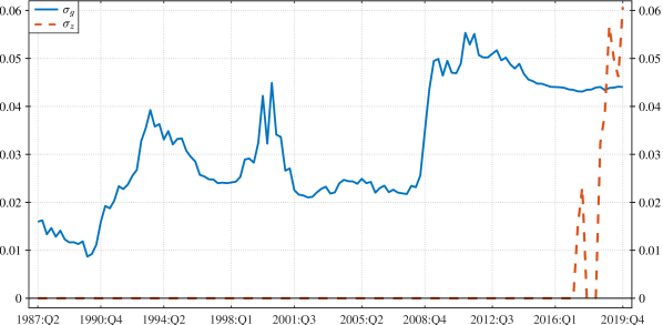
Figure 1: Recursive ML estimates of $\sigma_{g}$ and $\sigma_{z}$ from HLW’s full model in (1) using HLW’s initial values for the state vector. These results are based on US data, using an expanding window of data from 1987:Q2 to 2019:Q4. The data were downloaded from FRED on the 28^th May 2020.

Figure 2: Sequence of $F(\tau)$ statistics from SW’s and HLW’s implementation of the structural break dummy variable regressions described in (12) and (14), respectively.

Table 1: Stage 2 parameter estimates for the US

$\bm{\theta}_{2}$	HLW.R-File	HLW$\left(\vbox to0.0pt{}\right.\n@space$$\hat{\sigma}_{g}^{\mathrm{MLE}}$$\left)\vbox to0.0pt{}\right.\n@space$	Correct	Correct $+\hskip 1.5pta_{0}$
$\hskip 8.53581pta_{y,1}$	$1.51438668$	$1.47605057$	$1.51817784$	$1.51186045$
$\hskip 8.53581pta_{y,2}$	$-0.57128595$	$-0.53488829$	$-0.57824253$	$-0.57230827$
$\hskip 8.53581pta_{r}$	$-0.07346174$	$-0.08402097$	$-0.06825241$	$-0.07164411$
$\hskip 8.53581pta_{0}$	$-0.38877981$	$-0.39331138$	—	$-0.04299913$
$\hskip 8.53581pta_{g}$	$0.75724701$	$0.79592000$	—	—
$\hskip 8.53581ptb_{\pi}$	$0.66838723$	$0.67179221$	$0.67465713$	$0.67160611$
$\hskip 8.53581ptb_{y}$	$0.07934934$	$0.07552146$	$0.07710993$	$0.08112417$
$\hskip 8.53581pt\sigma_{\tilde{y}}$	$0.33550730$	$0.32902106$	$0.34846403$	$0.34552731$
$\hskip 8.53581pt\sigma_{\pi}$	$0.78523542$	$0.78643123$	$0.78785015$	$0.78662062$
$\hskip 8.53581pt\sigma_{y^{\ast}}$	$0.56797409$	$0.56163865$	$0.56051398$	$0.56064660$
$\hskip 8.53581pt\sigma_{g}$ (implied)	$(0.03042073$)	$0.04275448$	$0.04348429$	$0.04606357$
$\hskip 8.53581pt\lambda_{g}$ (implied)	$0.05356007$	$(0.07612453$)	$(0.07757932$)	$(0.08216150$)

Log-likelihood -534.57461094 -534.37024579 -535.95791031 -535.57316476

Notes: This table reports parameter estimates of the various Stage 2 models. The first column (‘HLW.R-File’) lists the estimates obtained from Holston et al.’s (2017) R-Files, where $\lambda_{g}$ is fixed at the first stage estimate and $\sigma_{g}$ is implied from the Stage 1 signal-to-noise ratio $\lambda_{g}=\sigma_{g}/\sigma_{y^{\ast}}$. The second column (‘HLW($\hat{\sigma}_{g}^{\mathsf{MLE}}$)’) shows estimates of the same model, but with $\sigma_{g}$ computed by MLE together with the other parameters of HLW’s (misspecified) Stage 2 model shown in the right column block of (6). The third column (‘Correct’) provides estimates of the correct Stage 2 model defined in the left column block of (6), where $\sigma_{g}$ is again estimated directly by MLE. The last column (‘Correct + $a_{0}$’) shows estimates of the correct Stage 2 model when an additional intercept term is added to the specification. Values in round brackets give the implied values of $\sigma_{g}$ or $\lambda_{g}$ from the $\lambda_{g}=\sigma_{g}/\sigma_{y^{\ast}}$ relation when either $\lambda_{g}$ or $\sigma_{g}$ are estimated.

Figure 3: Sequence of $F(\tau)$ statistics from HLW’s (misspecified) Stage 2 model and the correct Stage 2 model defined in the left and right columns blocks of (6) for the US. The red (HLW) and blue (SW) lines show respectively the $F(\tau)$ statistics of the two different implementations of the structural break regressions given in equations (15) to (18).

Table 2: Stage 2 MUE results of $\lambda_{z}$ with corresponding structural break test statistics for the US

Corresponding structural break test statistics ($p-$values in parenthesis) $L$   — 0.037097 (0.9450) 0.170077 (0.3350) 0.049609 (0.8750) 0.037097 (0.9450) 0.170077 (0.3350) MW 2.747739 3.850795 (0.0150) 1.159557 (0.2850) 0.326527 (0.8150) 0.251819 (0.8900) 0.977255 (0.3550) EW 2.553645 3.184074 (0.0100) 0.775920 (0.2800) 0.199023 (0.7900) 0.148746 (0.8750) 0.681178 (0.3250) QLR 12.398151 13.725281 (0.0050) 6.156285 (0.1450) 2.759496 (0.5900) 2.185052 (0.7200) 5.613296 (0.1850)

Notes: This table reports the Stage 2 MUEs of $\lambda_{z}$ and corresponding structural break statistics computed from the correct Stage 2 model and HLW’s (misspecified) Stage 2 model defined in the left and right columns of (6), respectively. The table is split into a left and right block corresponding to the two different implementations of the structural break regressions for each of the Stage 2 models defined in equations (15) to (18). The left block shows HLW’s implementation of the structural break regressions. The right block shows SW’s implementation. The table is further split into a top and bottom half. The top half shows the MUEs of $\lambda_{z}$. The bottom half lists the corresponding structural break test statistics. The results under (‘HLW.R-File’) report $\lambda_{z}$ estimates obtained from Holston et al.’s (2017) R-Files for HLW’s (misspecified) Stage 2 model. The (‘HLW($\hat{\sigma}_{g}^{\mathsf{MLE}}$)’) column lists estimates of the same model but with $\sigma_{g}$ estimated directly by MLE rather than from the first Stage $\lambda_{g}$. Results under the heading (‘Correct’) are for the correct Stage 2 model, where $\sigma_{g}$ is again estimated directly by MLE. The table lists results for all four structural break tests, namely, Nyblom’s (1989) $L$, MW, EW and QLR tests. Values in square brackets in the top part of the table are $90\%$ lower and upper confidence intervals (CIs). Values in parenthesis in the bottom part are $p-$values corresponding to SW’s structural break tests. Both, the CIs as well as the $p-$values, were obtained from Stock and Watson’s (1998) GAUSS files.

Table 3: Stage 3 parameter estimates for the US

Log-likelihood -536.48377160 -535.97760443 -535.97718006

Notes: This table reports the Stage 3 estimates. The first column (‘HLW.R-File’) gives the estimates from Holston et al.’s (2017) R-Files. The second column (‘MLE$(\sigma_{g}|\hat{\lambda}_{z}^{\mathrm{Correct}})$’) shows estimates of $\lambda_{z}$ from the correct Stage 2 model and SW’s implementation of the structural break regressions in (18) (based on the EW structural break test), where $\sigma_{g}$ is again estimated by MLE. The last column (‘MLE$(\sigma_{g},\sigma_{z})$’) reports estimates where all parameters, including $(\sigma_{g},\sigma_{z})$, are computed directly by MLE. Values in round brackets give the implied $(\sigma_{g},\sigma_{z})$ or $(\lambda_{g},\lambda_{z})$ values constructed from the signal-to-noise ratios $\lambda_{g}=\sigma_{g}/\sigma_{y^{\ast}}$ and $\lambda_{z}=a_{r}\sigma_{z}/\sigma_{\tilde{y}}$.

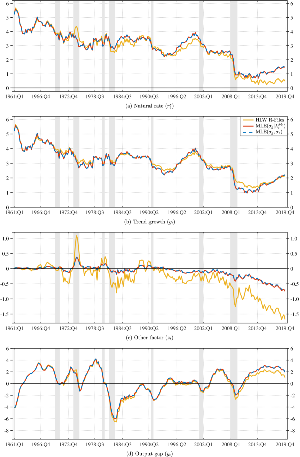
Figure 4: Filtered estimates of the natural rate $r^{\ast}_{t}$, annualized trend growth $g_{t}$, other factor $z_{t}$, and the output gap (cycle) variable $\tilde{y}_{t}$ for the US.

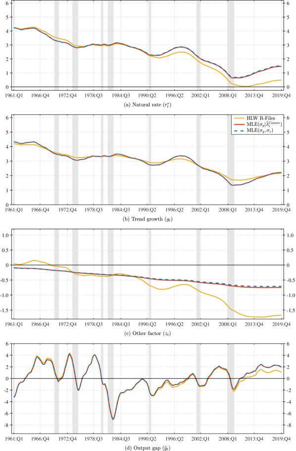
Figure 5: Smoothed estimates of the natural rate $r^{\ast}_{t}$, annualized trend growth $g_{t}$, other factor $z_{t}$, and the output gap (cycle) variable $\tilde{y}_{t}$ for the US.

Table 4: Stage 2 parameter estimates for the Euro Area

Log-likelihood -422.30013304 -421.13354157 -421.17804744 -421.13660601

Notes: This table reports parameter estimates of the various Stage 2 models. The first column (‘HLW.R-File’) lists the estimates obtained from Holston et al.’s (2017) R-Files, where $\lambda_{g}$ is fixed at the first stage estimate and $\sigma_{g}$ is implied from the Stage 1 signal-to-noise ratio $\lambda_{g}=\sigma_{g}/\sigma_{y^{\ast}}$. The second column (‘HLW($\hat{\sigma}_{g}^{\mathsf{MLE}}$)’) shows estimates of the same model, but with $\sigma_{g}$ computed by MLE together with the other parameters of HLW’s (misspecified) Stage 2 model shown in the right column block of (6). The third column (‘Correct’) provides estimates of the correct Stage 2 model defined in the left column block of (6), where $\sigma_{g}$ is again estimated directly by MLE. The last column (‘Correct + $a_{0}$’) shows estimates of the correct Stage 2 model when an additional intercept term is added to the specification. Values in round brackets give the implied values of $\sigma_{g}$ or $\lambda_{g}$ from the $\lambda_{g}=\sigma_{g}/\sigma_{y^{\ast}}$ relation when either $\lambda_{g}$ or $\sigma_{g}$ are estimated.

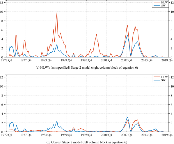
Figure 6: Sequence of $F(\tau)$ statistics from HLW’s (misspecified) Stage 2 model and the correct Stage 2 model defined in the left and right columns blocks of (6) for the Euro Area. The red (HLW) and blue (SW) lines show respectively the $F(\tau)$ statistics of the two different implementations of the structural break regressions given in equations (15) to (18).

Table 5: Stage 2 MUE results of $\lambda_{z}$ with corresponding structural break test statistics for the Euro Area

Corresponding structural break test statistics ($p-$values in parenthesis) $L$   — 0.067682 (0.7650) 0.068424 (0.7600) 0.097108 (0.5950) 0.067682 (0.7650) 0.068424 (0.7600) MW 1.493978 1.270378 (0.2500) 0.351069 (0.7900) 0.622436 (0.5450) 0.454903 (0.6850) 0.455205 (0.6850) EW 1.525650 1.090316 (0.1750) 0.226251 (0.7500) 0.474062 (0.4550) 0.300121 (0.6400) 0.292027 (0.6500) QLR 9.882686 8.878605 (0.0450) 2.652280 (0.6150) 4.796794 (0.2650) 3.454149 (0.4500) 3.257853 (0.4900)

Notes: This table reports the Stage 2 MUEs of $\lambda_{z}$ and corresponding structural break statistics computed from the correct Stage 2 model and HLW’s (misspecified) Stage 2 model defined in the left and right columns of (6), respectively. The table is split into a left and right block corresponding to the two different implementations of the structural break regressions for each of the Stage 2 models defined in equations (15) to (18). The left block shows HLW’s implementation of the structural break regressions. The right block shows SW’s implementation. The table is further split into a top and bottom half. The top half shows the MUEs of $\lambda_{z}$. The bottom half lists the corresponding structural break test statistics. The results under (‘HLW.R-File’) report $\lambda_{z}$ estimates obtained from Holston et al.’s (2017) R-Files for HLW’s (misspecified) Stage 2 model. The (‘HLW($\hat{\sigma}_{g}^{\mathsf{MLE}}$)’) column lists estimates of the same model but with $\sigma_{g}$ estimated directly by MLE rather than from the first Stage $\lambda_{g}$. Results under the heading (‘Correct’) are for the correct Stage 2 model, where $\sigma_{g}$ is again estimated directly by MLE. The table lists results for all four structural break tests, namely, Nyblom’s (1989) $L$, MW, EW and QLR tests. Values in square brackets in the top part of the table are $90\%$ lower and upper confidence intervals (CIs). Values in parenthesis in the bottom part are $p-$values corresponding to SW’s structural break tests. Both, the CIs as well as the $p-$values, were obtained from Stock and Watson’s (1998) GAUSS files.

Table 6: Stage 3 parameter estimates for the Euro Area

Log-likelihood -422.87276090 -421.23654260 -421.23654260

Notes: This table reports the Stage 3 estimates. The first column (‘HLW.R-File’) gives the estimates from Holston et al.’s (2017) R-Files. The second column (‘MLE$(\sigma_{g}|\hat{\lambda}_{z}^{\mathrm{Correct}})$’) shows estimates of $\lambda_{z}$ from the correct Stage 2 model and SW’s implementation of the structural break regressions in (18) (based on the EW structural break test), where $\sigma_{g}$ is again estimated by MLE. The last column (‘MLE$(\sigma_{g},\sigma_{z})$’) reports estimates where all parameters, including $(\sigma_{g},\sigma_{z})$, are computed directly by MLE. Values in round brackets give the implied $(\sigma_{g},\sigma_{z})$ or $(\lambda_{g},\lambda_{z})$ values constructed from the signal-to-noise ratios $\lambda_{g}=\sigma_{g}/\sigma_{y^{\ast}}$ and $\lambda_{z}=a_{r}\sigma_{z}/\sigma_{\tilde{y}}$.

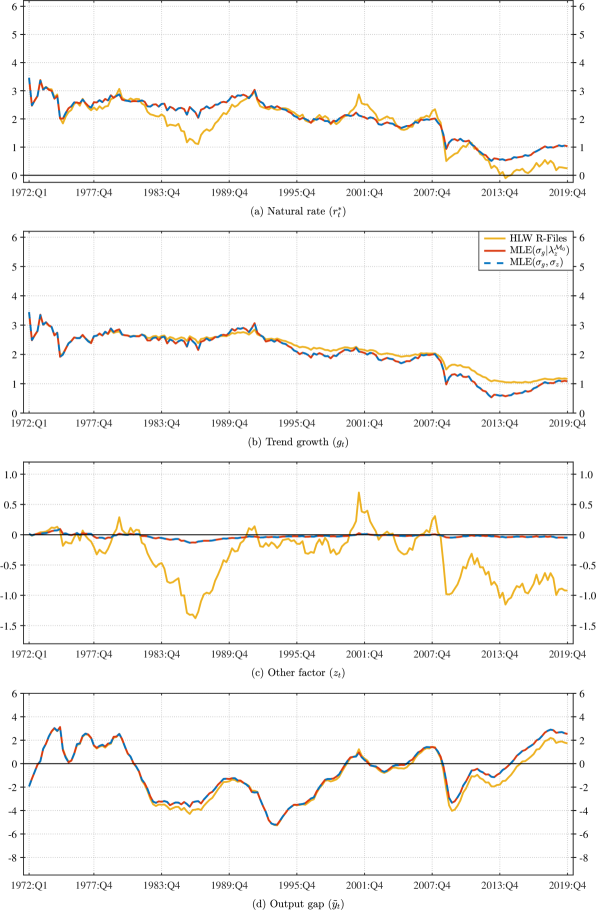
Figure 7: Filtered estimates of the natural rate $r^{\ast}_{t}$, annualized trend growth $g_{t}$, other factor $z_{t}$, and the output gap (cycle) variable $\tilde{y}_{t}$ for the Euro Area

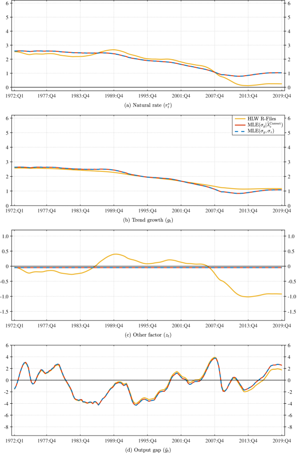
Figure 8: Smoothed estimates of the natural rate $r^{\ast}_{t}$, annualized trend growth $g_{t}$, other factor $z_{t}$, and the output gap (cycle) variable $\tilde{y}_{t}$ for the Euro Area

Table 7: Stage 2 parameter estimates for the UK

Log-likelihood -877.75517435 -877.74815473 -877.76354886 -877.74887189

Notes: This table reports parameter estimates of the various Stage 2 models. The first column (‘HLW.R-File’) lists the estimates obtained from Holston et al.’s (2017) R-Files, where $\lambda_{g}$ is fixed at the first stage estimate and $\sigma_{g}$ is implied from the Stage 1 signal-to-noise ratio $\lambda_{g}=\sigma_{g}/\sigma_{y^{\ast}}$. The second column (‘HLW($\hat{\sigma}_{g}^{\mathsf{MLE}}$)’) shows estimates of the same model, but with $\sigma_{g}$ computed by MLE together with the other parameters of HLW’s (misspecified) Stage 2 model shown in the right column block of (6). The third column (‘Correct’) provides estimates of the correct Stage 2 model defined in the left column block of (6), where $\sigma_{g}$ is again estimated directly by MLE. The last column (‘Correct + $a_{0}$’) shows estimates of the correct Stage 2 model when an additional intercept term is added to the specification. Values in round brackets give the implied values of $\sigma_{g}$ or $\lambda_{g}$ from the $\lambda_{g}=\sigma_{g}/\sigma_{y^{\ast}}$ relation when either $\lambda_{g}$ or $\sigma_{g}$ are estimated.

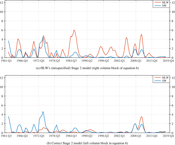
Figure 9: Sequence of $F(\tau)$ statistics from HLW’s (misspecified) Stage 2 model and the correct Stage 2 model defined in the left and right columns blocks of (6) for the UK. The red (HLW) and blue (SW) lines show respectively the $F(\tau)$ statistics of the two different implementations of the structural break regressions given in equations (15) to (18).

Table 8: Stage 2 MUE results of $\lambda_{z}$ with corresponding structural break test statistics for the UK

Corresponding structural break test statistics ($p-$values in parenthesis) $L$   — 0.080184 (0.6900) 0.081772 (0.6800) 0.079305 (0.6900) 0.080184 (0.6900) 0.081772 (0.6800) MW 1.295177 1.319085 (0.2400) 0.309463 (0.8300) 0.540538 (0.6100) 0.546107 (0.6050) 0.555764 (0.6000) EW 0.984618 1.021807 (0.1900) 0.210029 (0.7750) 0.392172 (0.5350) 0.397701 (0.5300) 0.409986 (0.5150) QLR 5.993069 6.261263 (0.1400) 3.541260 (0.4350) 4.408113 (0.3050) 4.476559 (0.2950) 4.619930 (0.2800)

Notes: This table reports the Stage 2 MUEs of $\lambda_{z}$ and corresponding structural break statistics computed from the correct Stage 2 model and HLW’s (misspecified) Stage 2 model defined in the left and right columns of (6), respectively. The table is split into a left and right block corresponding to the two different implementations of the structural break regressions for each of the Stage 2 models defined in equations (15) to (18). The left block shows HLW’s implementation of the structural break regressions. The right block shows SW’s implementation. The table is further split into a top and bottom half. The top half shows the MUEs of $\lambda_{z}$. The bottom half lists the corresponding structural break test statistics. The results under (‘HLW.R-File’) report $\lambda_{z}$ estimates obtained from Holston et al.’s (2017) R-Files for HLW’s (misspecified) Stage 2 model. The (‘HLW($\hat{\sigma}_{g}^{\mathsf{MLE}}$)’) column lists estimates of the same model but with $\sigma_{g}$ estimated directly by MLE rather than from the first Stage $\lambda_{g}$. Results under the heading (‘Correct’) are for the correct Stage 2 model, where $\sigma_{g}$ is again estimated directly by MLE. The table lists results for all four structural break tests, namely, Nyblom’s (1989) $L$, MW, EW and QLR tests. Values in square brackets in the top part of the table are $90\%$ lower and upper confidence intervals (CIs). Values in parenthesis in the bottom part are $p-$values corresponding to SW’s structural break tests. Both, the CIs as well as the $p-$values, were obtained from Stock and Watson’s (1998) GAUSS files.

Table 9: Stage 3 parameter estimates for the UK

Log-likelihood -877.97896968 -877.77522874 -877.77522874

Notes: This table reports the Stage 3 estimates. The first column (‘HLW.R-File’) gives the estimates from Holston et al.’s (2017) R-Files. The second column (‘MLE$(\sigma_{g}|\hat{\lambda}_{z}^{\mathrm{Correct}})$’) shows estimates of $\lambda_{z}$ from the correct Stage 2 model and SW’s implementation of the structural break regressions in (18) (based on the EW structural break test), where $\sigma_{g}$ is again estimated by MLE. The last column (‘MLE$(\sigma_{g},\sigma_{z})$’) reports estimates where all parameters, including $(\sigma_{g},\sigma_{z})$, are computed directly by MLE. Values in round brackets give the implied $(\sigma_{g},\sigma_{z})$ or $(\lambda_{g},\lambda_{z})$ values constructed from the signal-to-noise ratios $\lambda_{g}=\sigma_{g}/\sigma_{y^{\ast}}$ and $\lambda_{z}=a_{r}\sigma_{z}/\sigma_{\tilde{y}}$.

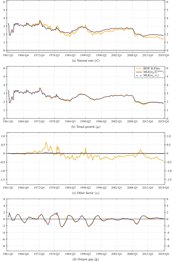
Figure 10: Filtered estimates of the natural rate $r^{\ast}_{t}$, annualized trend growth $g_{t}$, other factor $z_{t}$, and the output gap (cycle) variable $\tilde{y}_{t}$ for the UK

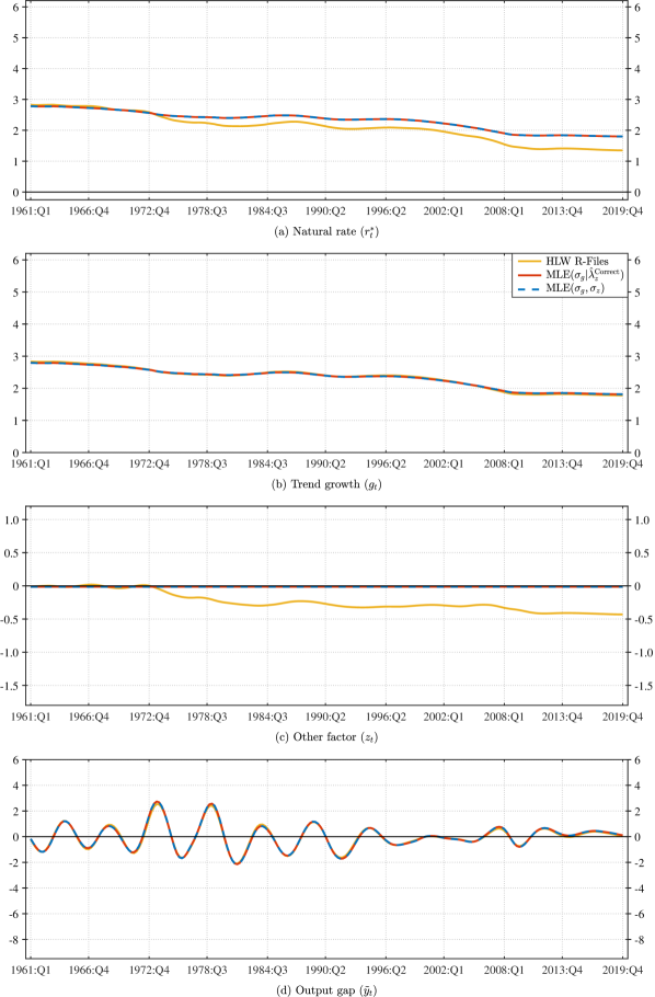
Figure 11: Smoothed estimates of the natural rate $r^{\ast}_{t}$, annualized trend growth $g_{t}$, other factor $z_{t}$, and the output gap (cycle) variable $\tilde{y}_{t}$ for the UK

Table 10: Stage 2 parameter estimates for Canada

Log-likelihood -679.90156186 -679.87545118 -679.94373632 -679.94347472

Notes: This table reports parameter estimates of the various Stage 2 models. The first column (‘HLW.R-File’) lists the estimates obtained from Holston et al.’s (2017) R-Files, where $\lambda_{g}$ is fixed at the first stage estimate and $\sigma_{g}$ is implied from the Stage 1 signal-to-noise ratio $\lambda_{g}=\sigma_{g}/\sigma_{y^{\ast}}$. The second column (‘HLW($\hat{\sigma}_{g}^{\mathsf{MLE}}$)’) shows estimates of the same model, but with $\sigma_{g}$ computed by MLE together with the other parameters of HLW’s (misspecified) Stage 2 model shown in the right column block of (6). The third column (‘Correct’) provides estimates of the correct Stage 2 model defined in the left column block of (6), where $\sigma_{g}$ is again estimated directly by MLE. The last column (‘Correct + $a_{0}$’) shows estimates of the correct Stage 2 model when an additional intercept term is added to the specification. Values in round brackets give the implied values of $\sigma_{g}$ or $\lambda_{g}$ from the $\lambda_{g}=\sigma_{g}/\sigma_{y^{\ast}}$ relation when either $\lambda_{g}$ or $\sigma_{g}$ are estimated.

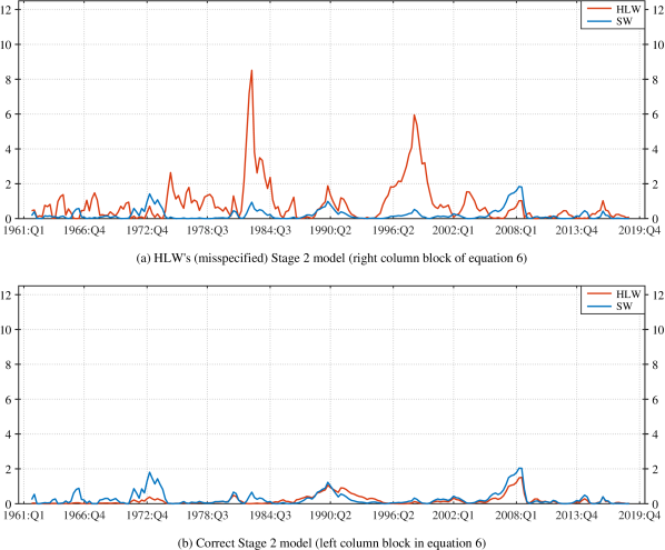
Figure 12: Sequence of $F(\tau)$ statistics from HLW’s (misspecified) Stage 2 model and the correct Stage 2 model defined in the left and right columns blocks of (6) for Canada. The red (HLW) and blue (SW) lines show respectively the $F(\tau)$ statistics of the two different implementations of the structural break regressions given in equations (15) to (18).

Table 11: Stage 2 MUE results of $\lambda_{z}$ with corresponding structural break test statistics for Canada

Corresponding structural break test statistics ($p-$values in parenthesis) $L$   — 0.037529 (0.9450) 0.048128 (0.8850) 0.038851 (0.9350) 0.037529 (0.9450) 0.048128 (0.8850) MW 0.833493 0.824762 (0.4200) 0.182530 (0.9550) 0.221949 (0.9200) 0.214878 (0.9250) 0.278728 (0.8650) EW 0.801254 0.761333 (0.2900) 0.101482 (0.9500) 0.126872 (0.9100) 0.122280 (0.9200) 0.161823 (0.8550) QLR 8.513039 8.272703 (0.0550) 1.514397 (0.8850) 1.842522 (0.8050) 1.793354 (0.8200) 2.040637 (0.7600)

Notes: This table reports the Stage 2 MUEs of $\lambda_{z}$ and corresponding structural break statistics computed from the correct Stage 2 model and HLW’s (misspecified) Stage 2 model defined in the left and right columns of (6), respectively. The table is split into a left and right block corresponding to the two different implementations of the structural break regressions for each of the Stage 2 models defined in equations (15) to (18). The left block shows HLW’s implementation of the structural break regressions. The right block shows SW’s implementation. The table is further split into a top and bottom half. The top half shows the MUEs of $\lambda_{z}$. The bottom half lists the corresponding structural break test statistics. The results under (‘HLW.R-File’) report $\lambda_{z}$ estimates obtained from Holston et al.’s (2017) R-Files for HLW’s (misspecified) Stage 2 model. The (‘HLW($\hat{\sigma}_{g}^{\mathsf{MLE}}$)’) column lists estimates of the same model but with $\sigma_{g}$ estimated directly by MLE rather than from the first Stage $\lambda_{g}$. Results under the heading (‘Correct’) are for the correct Stage 2 model, where $\sigma_{g}$ is again estimated directly by MLE. The table lists results for all four structural break tests, namely, Nyblom’s (1989) $L$, MW, EW and QLR tests. Values in square brackets in the top part of the table are $90\%$ lower and upper confidence intervals (CIs). Values in parenthesis in the bottom part are $p-$values corresponding to SW’s structural break tests. Both, the CIs as well as the $p-$values, were obtained from Stock and Watson’s (1998) GAUSS files.

Table 12: Stage 3 parameter estimates for Canada

Log-likelihood -680.25212417 -680.00345718 -680.00345718

Notes: This table reports the Stage 3 estimates. The first column (‘HLW.R-File’) gives the estimates from Holston et al.’s (2017) R-Files. The second column (‘MLE$(\sigma_{g}|\hat{\lambda}_{z}^{\mathrm{Correct}})$’) shows estimates of $\lambda_{z}$ from the correct Stage 2 model and SW’s implementation of the structural break regressions in (18) (based on the EW structural break test), where $\sigma_{g}$ is again estimated by MLE. The last column (‘MLE$(\sigma_{g},\sigma_{z})$’) reports estimates where all parameters, including $(\sigma_{g},\sigma_{z})$, are computed directly by MLE. Values in round brackets give the implied $(\sigma_{g},\sigma_{z})$ or $(\lambda_{g},\lambda_{z})$ values constructed from the signal-to-noise ratios $\lambda_{g}=\sigma_{g}/\sigma_{y^{\ast}}$ and $\lambda_{z}=a_{r}\sigma_{z}/\sigma_{\tilde{y}}$.

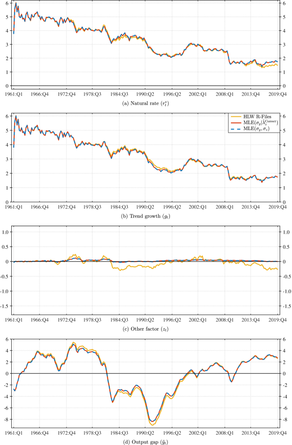
Figure 13: Filtered estimates of the natural rate $r^{\ast}_{t}$, annualized trend growth $g_{t}$, other factor $z_{t}$, and the output gap (cycle) variable $\tilde{y}_{t}$ for Canada

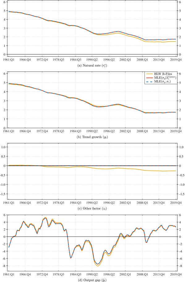
Figure 14: Smoothed estimates of the natural rate $r^{\ast}_{t}$, annualized trend growth $g_{t}$, other factor $z_{t}$, and the output gap (cycle) variable $\tilde{y}_{t}$ for Canada

References

- Andrews and Ploberger (1994) Andrews, Donald W. K. and Werner Ploberger (1994): “Optimal Tests when a Nuisance Parameter is Present only under the Alternative,” Econometrica, 62(6), 1383–1414.
- Benes. et al. (2010) Benes., J., K. Clinton, R. Garcia-Saltos, M. Johnson, D. Laxton, P. Manchev and Troy Matheson (2010): “Estimating Potential Output with a Multivariate Filter,” IMF Working Paper No. 10/285, International Monetary Fund. Available from: https://www.imf.org/external/pubs/ft/wp/2010/wp10285.pdf.
- Berger and Kempa (2019) Berger, Tino and Bernd Kempa (2019): “Testing for time variation in the natural rate of interest,” Journal of Applied Econometrics, 34(5), 836–842.
- Buncic (2021) Buncic, Daniel (2021): “Econometric Issues with Laubach and Williams Estimates of the Natural Rate of Interest,” Sveriges Riksbank Working Paper No. 397, Sveriges Riksbank. Available from: https://www.riksbank.se/globalassets/media/rapporter/working-papers/2019/no.-397-econometric-issues-with-laubach-and-williams-estimates-of-the-natural-rate-of-interest2.pdf.
- Buncic and Melecky (2008) Buncic, Daniel and Martin Melecky (2008): “An Estimated New Keynesian Policy Model for Australia,” The Economic Record, 84(264), 1–16.
- Chow (1960) Chow, Gregory C. (1960): “Tests of Equality between Sets of Coefficients in two Linear Regressions,” Econometrica, 28(3), 591–605.
- Clark (1987) Clark, Peter K. (1987): “The Cyclical Component of U.S. Economic Activity,” Quarterly Journal of Economics, 102(4), 797–814.
- Frühwirth-Schnatter and Wagner (2010) Frühwirth-Schnatter, Sylvia and Helga Wagner (2010): “Stochastic model specification search for Gaussian and partial non-Gaussian state space models,” Journal of Econometrics, 154(1), 85–100.
- Galí (2015) Galí, Jordi (2015): Monetary policy, inflation, and the business cycle: an introduction to the new Keynesian framework and its applications, 2nd Edition, Princeton University Press.
- Holston et al. (2017) Holston, Kathryn, Thomas Laubach and John C. Williams (2017): “Measuring the Natural Rate of Interest: International Trends and Determinants,” Journal of International Economics, 108(Supplement 1), S59–S75.
- Kiley (2020) Kiley, Michael T. (2020): “What Can the Data Tell us about the Equilibrium Real Interest Rate,” International Journal of Central Banking, 16(3), 181–209.
- Laubach and Williams (2003) Laubach, Thomas and John C. Williams (2003): “Measuring the Natural Rate of Interest,” Review of Economics and Statistics, 85(4), 1063–1070.
- Lewis and Vazquez-Grande (2018) Lewis, Kurt F. and Francisco Vazquez-Grande (2018): “Measuring the natural rate of interest: A note on transitory shocks,” Journal of Applied Econometrics, 34(3), 425–436.
- Nyblom (1989) Nyblom, Jukka (1989): “Testing for the Constancy of Parameters over Time,” Journal of the American Statistical Association, 84(405), 223–230.
- Quandt (1960) Quandt, Richard E. (1960): “Tests of the Hypothesis that a Linear Regression System obeys two Separate Regimes,” Journal of the American Statistical Association, 55(290), 324–330.
- Stock and Watson (1998) Stock, James H. and Mark W. Watson (1998): “Median Unbiased Estimation of Coefficient Variance in a Time-Varying Parameter Model,” Journal of the American Statistical Association, 93(441), 349–358.