Robustifying Conditional Portfolio Decisions
via Optimal Transport

Abstract.

We propose a data-driven portfolio selection model that integrates side information, conditional estimation and robustness using the framework of distributionally robust optimization. Conditioning on the observed side information, the portfolio manager solves an allocation problem that minimizes the worst-case conditional risk-return trade-off, subject to all possible perturbations of the covariate-return probability distribution in an optimal transport ambiguity set. Despite the non-linearity of the objective function in the probability measure, we show that the distributionally robust portfolio allocation with side information problem can be reformulated as a finite-dimensional optimization problem. If portfolio decisions are made based on either the mean-variance or the mean-Conditional Value-at-Risk criterion, the resulting reformulation can be further simplified to second-order or semi-definite cone programs. Empirical studies in the US equity market demonstrate the advantage of our integrative framework against other benchmarks.

1. Introduction

We study distributionally robust portfolio decision rules which are informed by conditioning on observed side information. In the presence of contextual information which might be relevant for predicting future returns, our objective is to direct the statistical task (i.e., conditional estimation) towards the downstream task of selecting a portfolio which is robust to distributional shifts (including on local conditioning). Our ultimate goal is to provide a tractable, non-parametric, data-driven approach which bypasses the need for computing global conditional expectations. At the same time, our framework is flexible to accommodate a wide range of portfolio optimization selection criteria, as well as extend to other diverse applications. In order to explain our methodology and contribution in detail, let us consider a conventional single-period portfolio optimization selection problem of the form

$$\min\limits_{\alpha\in\mathcal{A}}~{}\mathcal{R}_{\mathbb{P}}[Y^{\top}\alpha]-\eta\cdot\mathds{E}_{\mathbb{P}}[Y^{\top}\alpha],$$

where the real-valued vector $\alpha$ denotes the portfolio allocation choice within a feasible region $\mathcal{A}$, and the random vector $Y$ denotes the assets’ future return under a probability measure $\mathbb{P}$. The return of the portfolio is denoted by $Y^{\top}\alpha$, while $\mathcal{R}_{\mathbb{P}}[\cdot]$ captures the risk associated with $\alpha$, and $\eta\geq 0$ is a parameter that weights the preference between the portfolio return and the associated risk.

Different choices of the measure of risk $\mathcal{R}_{\mathbb{P}}[\cdot]$ lead to different portfolio optimization models, including the mean-variance model [56], the mean-standard deviation model [49], the mean-Value-at-Risk model [8], and the mean-Conditional Value-at-Risk (CVaR) model [70]. The measure of risk $\mathcal{R}_{\mathbb{P}}[\cdot]$ often is chosen to belong to certain classes in order to induce desirable properties. For instance, the class of coherent risk measures [3] or the class of convex risk measures [38] are examples of risk measure classes which are often used in portfolio optimization [55]. In our setting, we consider a family of risk measures which admits a stochastic optimization representation of the form $\mathcal{R}_{\mathbb{P}}[Y^{\top}\alpha]=\min_{\beta\in\mathcal{B}}\mathds{E}_{\mathbb{P}}[r(Y^{\top}\alpha,\beta)]$ for some auxiliary function $r$ and finite-dimensional statistical variable $\beta$ residing within an appropriate feasible region $\mathcal{B}$. Hence, we focus on a generic portfolio allocation that minimizes an expected loss of the form

$$\min\limits_{\alpha\in\mathcal{A},~{}\beta\in\mathcal{B}}~{}\mathds{E}_{\mathbb{P}}[\ell(Y,\alpha,\beta)],\qquad\ell(Y,\alpha,\beta)\triangleq r(Y^{\top}\alpha,\beta)-\eta\cdot Y^{\top}\alpha.$$ (1)

In problem (1), optimizing over $\beta$ characterizes the improvement of risk estimation, which is entangled with the procedure of finding the optimal portfolio allocation $\alpha$. For example, consider when $\mathcal{R}_{\mathbb{P}}$ is the variance of the portfolio return, then by setting $\mathcal{B}=\mathbb{R}$ and choosing $\ell$ as a quadratic function, we can rewrite the variance in the form $\mathcal{R}_{\mathbb{P}}[Y^{\top}\alpha]=\min_{\beta\in\mathbb{R}}~{}\mathds{E}_{\mathbb{P}}[(Y^{\top}\alpha-\beta)^{2}]$. This further implies that the optimal solution of $\beta$ coincides with the expected return $\mathds{E}_{\mathbb{P}}[Y^{\top}\alpha]$, and one thus can view $\beta$ as an auxiliary statistical variable representing the estimation of the expected portfolio return.

Despite the simplicity and popularity of the portfolio optimization models (1), they are challenging to solve because the distribution $\mathbb{P}$ of the random stock returns is unknown to the portfolio managers. To overcome this issue, problem (1) is usually solved by resorting to a plug-in estimator $\widehat{\mathbb{P}}$ of $\mathbb{P}$, and this estimator is usually inferred from the available data. Unfortunately, solving (1) using an estimated distribution $\widehat{\mathbb{P}}$ may amplify the statistical estimation error. The corresponding portfolio allocation is vulnerable to the estimation errors of the input: even small changes in the input parameters can result in large changes in the weights of the optimal portfolio [22, 20]. Consequently, in terms of out-of-sample performance, the advantage of deploying the optimal portfolio weights is overwhelmed by the offset of estimation error [26]. To mitigate the estimation error, one may resort, at least, to the following two strategies:

1. reduce the estimation bias by incorporating side information into the portfolio allocation problems;

2. diminish the impact of estimation variance by employing robust portfolio optimization models.

Both above-mentioned strategies have led to successful stories. Starting from the capital asset-pricing model [74, 13], numerous studies exploit side information to explain and/or predict the cross-sectional variation of the stock returns. The predictive side information may include macro-economic factors [37], firms’ financial statements [34] and historical trading data [43]. Alternatively, robust optimization formulations are applied to the portfolio allocation tasks to alleviate the impact of statistical error due to input uncertainty [64, 24, 85].

In this paper, we endeavor to unify both strategies of leveraging side information and enhancing robustness. In order to incorporate the side information into portfolio allocation, we use a random vector $X$ to denote the side information that is correlated with the stock return $Y$, and consider the following conditional stochastic optimization (CSO) problem:

$$\min\limits_{\alpha\in\mathcal{A},~{}\beta\in\mathcal{B}}~{}\mathds{E}_{\mathbb{P}}[\ell(Y,\alpha,\beta)|X\in\mathcal{N}],$$ (2)

where the set $\mathcal{N}$ represents our prior (or most current) knowledge about the covariate $X$. In problem (2), the distribution $\mathbb{P}$ is now lifted to a joint distribution between the covariate $X$ and the return $Y$. Problem (2) is thus a joint portfolio allocation (over $\alpha$) and statistical estimation (over $\beta$) problem, that minimizes the conditional expected loss of the portfolio, given that the outcome of $X$ belongs to a set $\mathcal{N}$. To promote robust solutions and to hedge against the estimation error of $\mathbb{P}$, we will apply the distributionally robust framework. Instead of assessing the expected loss with respect to a single distribution, the distributionally robust formulation minimizes the expected conditional loss uniformly over a distributional ambiguity set that represents the portfolio managers’ ambiguity regarding the underlying distribution $\mathbb{P}$.

We propose a data-driven portfolio optimization framework that simultaneously exploits side information and robustifies over sampling error and model misspecification. We formulate the distributionally robust portfolio optimization problem with side information as

$$\min\limits_{\alpha\in\mathcal{A},~{}\beta\in\mathcal{B}}~{}\sup\limits_{\mathbb{Q}\in\mathbb{B},\mathbb{Q}(X\in\mathcal{N})\geq\varepsilon}~{}\mathds{E}_{\mathbb{Q}}[\ell(Y,\alpha,\beta)|X\in\mathcal{N}].$$ (3)

We can view the min-max problem (3) as a two-player zero-sum game: the portfolio manager chooses the portfolio allocation $\alpha$ and the estimation parameters $\beta$ so as to minimize the conditional expected loss, while the fictitious adversary chooses the joint distribution $\mathbb{Q}$ of $(X,Y)$ so as to maximize the incurring loss. A typical choice of the ambiguity set $\mathbb{B}$ is a neighborhood around a nominal distribution $\widehat{\mathbb{P}}$. In a data-driven setting, a popular choice of $\widehat{\mathbb{P}}$ is the empirical distribution, defined as a uniform distribution supported on the available data. As such, the data influences the optimization problem (3) via the channel of the ambiguity set prescription. Given $\varepsilon$ as an input parameter, the constraint $\mathbb{Q}(X\in\mathcal{N})\geq\varepsilon$ is a shorthand for $\mathbb{Q}((X,Y)\in\mathcal{N}\times\mathcal{Y})\geq\varepsilon$, and it controls the probability mass requirement on the set $\mathcal{N}\times\mathcal{Y}$ and avoids conditioning on sets of measure zero. In the limit, we also will study the case $\mathbb{Q}(X\in\mathcal{N})>0$ with strict inequality.

Intuitively, one can describe problem (3) as a zero-sum game between two players. The outer player is the statistical portfolio manager who optimizes over the allocation $\alpha$ and the estimator $\beta$ in order to minimize the conditional expected loss, and the inner player can be regarded as a fictitious adversary whose goal is to increase the resulting loss by choosing an adversarial distribution.

Our formulation (3) has several benefits. First, our model is an end-to-end framework that directly generates investment decisions using data. This approach, in the same spirit as [51] and [27], integrates the sequential pipeline of return prediction and portfolio optimization, which is conventionally employed by portfolio managers. Therefore, our model, which consolidates return prediction and portfolio optimization, directly minimizes the conditional expected loss instead of the prediction error of return. Second, the robustness of the random return is directed by the portfolio choice. Indeed, the adversary who solves the supremum problem in (3) will aim to maximize the portfolio loss, and not the statistical loss. Thirdly, our proposed model does not require imposing any parametric family for prediction, and thus it reduces the risk of model misspecification (see [79, 33] for examples of how this risk is typically mitigated).

1.1. Main Contributions

We study a robust portfolio optimization strategy that integrates conditional estimation and decision-making. This strategy leverages the side information to improve the ex-ante return prediction. Additionally, it also robustifies over estimation error in order to improve the out-of-sample performance of the portfolio allocation. Our contributions are summarized as follows.

1. We present a comprehensive modelling framework for distributionally robust optimization for conditional decision-making, which provides flexibilities for selecting different conditional set and adjusting probability mass requirement. We study specifically the case where the set $\mathbb{B}$ will be prescribed using the notions of optimal transport, and we show that the qualitative behavior of the distributionally robust portfolio optimization problem with side information depends on whether the set $\mathcal{N}$ is a singleton, and whether the probability mass requirement $\varepsilon$ is zero.

2. We derive finite-dimensional reformulations of the distributionally robust portfolio optimization problem with side information. Further, we also provide tractable reformulations for the distributionally robust mean-variance problem and mean-CVaR problem as convex conic (second-order cone or semi-definite cone) problems. These tractable reformulations are particularly interesting given that the conditional expectation is a nonlinear function of the probability measure (thus not amenable to traditional reformulations based on semi-infinite linear programming duality arguments), and that minimizing the worst-case conditional expected loss is equivalent to a min-max optimization problem with a fractional objective function.

3. We conduct extensive numerical experiments in the US equity markets. The results demonstrate the advantage of the distributionally robust portfolio optimization formulation, which has a higher Sharpe ratio and a better quantile performance for the portfolio return when compared with other benchmarks.

The distributionally robust optimization problem with side information as presented in (3) is generic, and our contributions are related to the vast literature in estimation-informed decision-making tasks. Moreover, by an appropriate choice of the loss function $\ell$, the sets $(\mathcal{A},\mathcal{B},\mathcal{N})$ and the ambiguity set $\mathbb{B}$, the formulation (3) can be applied to many other problems in the field of operations research and management science such as supply chain management, transportation and energy planning. In this regard, we refer interested readers to Appendix E where we extend our mean-CVaR results to contextual two-stage stochastic linear programming.

1.2. Related Literature

We start this section by discussing existing work that exploits side information to enhance portfolio optimization. For applications of fundamental analysis, Fama and French leveraged market capitalization and price-earning ratio to construct the celebrated factor models [34, 35], which was later applied to portfolio optimization [19]; Pástor and Stambaugh [62] reported the evidence of equity risk premium due to illiquidity. For applications of technical indicators, examples include momentum factor [43, 60], implied volatility [28], short interest [69], and investor sentiment [5]. However, when comparing with our proposed approach, these methods are vulnerable to estimation errors.

There is a rich literature on distributionally robust portfolio optimization, with diverse choices of distributional ambiguity set or different objective functions. When the objective function involves Value-at-Risk or CVaR, previous studies employed the moment-based ambiguity set [41, 84, 42] and Wasserstein ambiguity set [57] to model the worst-case risk. For distributionally robust portfolio optimizations that maximize piecewise affine loss functions, see [59] for moment-based ambiguity set, and [21] for event-wise ambiguity set. For the distributionally robust mean-variance problem, Lobo and Boyd [53] and Delage and Ye [24] are among the earliest to consider the worst-case mean-variance model under moment ambiguity set. Other types of ambiguity sets, such as Wasserstein ambiguity set [64, 14], and optimal transport ambiguity set [18], are also studied afterwards. Due to the resemblance between Wasserstein distributionally robustification and norm regularization [15], the weight-constrained portfolio optimization problem [25] is also closely related to this stream of research aiming to boost the robustness of the optimal portfolio. Nevertheless, none of the aforementioned works considers how to incorporate side information and conditional estimation.

The conditional stochastic optimization (CSO) problem (2) is also related to the topic of decision-making with side information, which receives significant attraction recently. Ban and Rudin [6] applied weighted sample average approximation (SAA) with weights learned from kernel regression to learn the optimal decision in inventory management with covariate information. Bertsimas and Kallus [9] applied weighted SAA to solve the general CSO problem, in which the weight is learned from nonparametric estimator such as k-nearest neighbors, kernel regressions, and random forests. Bertsimas and McCord [10] generalized the approach of [9] to multistage decision-making problems. Kannan et al. [46] developed a residual based SAA method, where average residuals during training of the learning model are added on to a point prediction of response, which is used as a response sample within the SAA. An extension to heteroscedastic residuals is provided in [47]. Decision tree based approaches are also developed to solve CSO. Athey et al. [4] proposed the forest-based estimates for local parameter estimation, generalizing the original random forest algorithm with observations of side information; Kallus and Mao [45] generalized the idea to solve stochastic optimization problems with side information, in which they seek to minimize the expected loss instead of the prediction accuracy. Conditional chance constrained programming was also studied recently [68].

Recently, distributionally robust optimization (DRO) formulations are integrated into the CSO problem to improve the out-of-sample performance of the solutions [11, 12, 78]. For example, Kannan et al. [48] constructed a Wasserstein based uncertainty set over the empirical distribution of the residuals, robustifying their previous work [46]; Esteban-Pérez and Morales [32] leveraged some probability trimming methods and a partial mass transportation problem to model the distributionally robust CSO problem.

Despite some common characteristics in terms of methodology, such as the idea of using the theory of optimal transport to robustify the CSO problem, our paper is an independent contribution in comparison to [48] and [32]. There are two key differences between our model and that considered in [48]. Firstly, we integrate prediction and decision-making into a single optimization problem, while in [48] the prediction and the decision-making procedures are separated to simplify the problem. Secondly, the conditional side information is required to be a singleton set $X=x_{0}$ in [48], but our approach allows for a more flexible modelling of side information by conditioning on a more general event $X\in\mathcal{N}$. Our work is also distinct from Esteban-Pérez and Morales [32]. In contrast to [32], which employs probability trimmings to relax problem (3), we seek to provide an exact and tractable reformulation of the problem. Moreover, our approach tackles the optimal transport ambiguity set directly, and the results can be explained by picturing an adversary who perturbs the sample points in an intuitive manner.

Finally, this paper is a complete and comprehensive extension to our previous work [61], with a twofold improvement. On the one hand, this paper naturally unifies prediction and decision-making into a single DRO problem, while [61] solely considers the conditional estimation problem. On the other hand, this paper applies optimal transport distance to construct a more versatile class of distributional ambiguity set, whereas the ambiguity set in [61] is based on the type-$\infty$ Wasserstein distance. Even though the type-$\infty$ Wasserstein distance is also motivated by the theory of optimal transport, it behaves qualitatively different from a type-$p$ ($p<\infty$) Wasserstein distance. The pathway to resolve the distributionally robust optimization problems in this paper hence differs significantly from the techniques employed in [61]. Finally, this paper also enriches the emerging field of Wasserstein DRO, which has gained momentum recently thanks to its applicability in a wide spectrum of practical problems [15, 40, 82, 31, 57, 52, 30].

Notations. For any integer $M\geq 1$, we denote by $[M]$ the set of integers $\{1,\ldots,M\}$. For any $x\in\mathbb{R}$, we denote by $(x)^{+}=\max\{x,0\}$. We write $\mathbb{R}_{+}\triangleq[0,\infty)$ and $\mathbb{R}_{++}\triangleq(0,\infty)$. Let $\|\cdot\|_{p}$ denote the $l_{p}$-norm for $p\in[1,\infty]$. For any space $\mathcal{S}$ equipped with a Borel sigma-algebra $\mathcal{F}_{\mathcal{S}}$, $\mathcal{M}(\mathcal{S})$ is the space of all probability measures defined on $(\mathcal{S},\mathcal{F}_{\mathcal{S}})$. For any $s\in\mathcal{S}$, the Dirac’s delta measure corresponding to $s$ is denoted by $\delta_{s}$, i.e., for all $E\in\mathcal{F}_{\mathcal{S}}$, $\delta_{s}(E)=1$ if $s\in E$ and $\delta_{s}(E)=0$ if $s\notin E$. For any subset $E\subseteq\mathcal{S}$, let $\partial E$ denote the boundary of $E$, which is the closure of $E$ minus the interior of $E$. The cone of $m\times m$ real positive semi-definite matrices is denoted by $\mathbb{S}_{+}^{m}$. For $m\times m$ real symmetric matrices $A$ and $B$, we write $A\succeq B$ if and only if $A-B\in\mathbb{S}_{+}^{m}$. For a probability measure $\mathbb{P}$, let $\mathds{E}_{\mathbb{P}}[\cdot]$ denote the expectation under measure $\mathbb{P}$. We write $\mathbbm{1}_{\mathcal{S}}(\cdot)$ as the indicator function of the set $\mathcal{S}$, i.e., $\mathbbm{1}_{\mathcal{S}}(s)=1$ if $s\in\mathcal{S}$ and $0$, otherwise. Throughout, $\mathcal{X}$ denotes the covariate space and $\mathcal{Y}$ denotes the asset return space. The available data consist of $N$ samples, each sample is a pair of covariate-return denoted by $(\widehat{x}_{i},\widehat{y}_{i})\in\mathcal{X}\times\mathcal{Y}$.

All proofs are relegated to the appendix.

2. Problem Setup

We delineate in this section the details on our robustification of the conditional portfolio allocation problem. To this end, we will construct the ambiguity set using the optimal transport cost.

Definition 2.1 (Optimal transport cost).

Fix any integer $k$ and let $\Xi\subseteq\mathbb{R}^{k}$. Let $\mathbb{D}$ be a nonnegative and continuous function on $\Xi\times\Xi$. The optimal transport cost between two distributions $\mathbb{Q}_{1}$ and $\mathbb{Q}_{2}$ supported on $\Xi$ is defined as

$$\mathds{W}(\mathbb{Q}_{1},\mathbb{Q}_{2})\triangleq\min\left\{\mathds{E}_{\pi}[\mathbb{D}(\xi_{1},\xi_{2})]:\pi\in\Pi(\mathbb{Q}_{1},\mathbb{Q}_{2})\right\},$$

where $\Pi(\mathbb{Q}_{1},\mathbb{Q}_{2})$ is the set of all probability measures on $\Xi\times\Xi$ with marginals $\mathbb{Q}_{1}$ and $\mathbb{Q}_{2}$, respectively.

Intuitively, the optimal transport cost $\mathds{W}(\mathbb{Q}_{1},\mathbb{Q}_{2})$ computes the cheapest cost of transporting the mass from an initial distribution $\mathbb{Q}_{1}$ to a target distribution $\mathbb{Q}_{2}$, given a function $\mathbb{D}(\xi_{1},\xi_{2})$ prescribing the cost of transporting a unit of mass from position $\xi_{1}$ to position $\xi_{2}$. The function $\mathbb{D}$ is referred to as the ground transport cost function. The existence of an optimal joint distribution $\pi^{\star}$ that attains the minimal value in the definition is guaranteed by [80, Theorem 4.1]. The class of optimal transport cost is rich enough to encompass common probability metrics. In particular, if $\mathbb{D}$ is a metric on $\Xi$, then $\mathds{W}$ coincides with the type-1 Wasserstein distance. In this paper, we do not restrict the ground transportation cost $\mathbb{D}$ to be a metric, and as a consequence, $\mathds{W}$ is not necessarily a proper distance on the space of probability measure. Nevertheless, we will usually refer to $\mathds{W}$ as an optimal transport distance with a slight abuse of terminology. A comprehensive introduction to the theory of optimal transport can be found in [80].

We now consider the covariate space $\mathcal{X}$, equipped with a ground cost $\mathbb{D}_{\mathcal{X}}$, and the return space $\mathcal{Y}$, equipped with a ground cost $\mathbb{D}_{\mathcal{Y}}$. The joint sample space $\mathcal{X}\times\mathcal{Y}$ is endowed with a ground cost $\mathbb{D}$, which is additively separable using $\mathbb{D}_{\mathcal{X}}$ and $\mathbb{D}_{\mathcal{Y}}$. We suppose that the portfolio manager possesses $N$ historical data samples, where each sample is a pair of covariate-return $(\widehat{x}_{i},\widehat{y}_{i})\in\mathcal{X}\times\mathcal{Y}$. Using the optimal transport cost in Definition 2.1, we define the joint ambiguity set of the distributions of $(X,Y)$ as

$$\mathbb{B}_{\rho}=\left\{\mathbb{Q}\in\mathcal{M}(\mathcal{X}\times\mathcal{Y}):\mathds{W}(\mathbb{Q},\widehat{\mathbb{P}})\leq\rho\right\}.$$

The set $\mathbb{B}_{\rho}$ contains all distributions that are of optimal transport distance less than or equal to $\rho$ from the empirical distribution

$$\widehat{\mathbb{P}}\triangleq\frac{1}{N}\sum_{i\in[N]}\delta_{(\widehat{x}_{i},\widehat{y}_{i})},$$

defined as the distribution that makes every member of the dataset $(\widehat{x}_{i},\widehat{y}_{i})_{i=1}^{N}$ equiprobable. In this form, $\mathbb{B}_{\rho}$ is a non-parametric ambiguity set. We propose to solve the distributionally robust conditional portfolio allocation problem

$$\min\limits_{\alpha\in\mathcal{A},~{}\beta\in\mathcal{B}}~{}\sup\limits_{\mathbb{Q}\in\mathbb{B}_{\rho},\mathbb{Q}(X\in\mathcal{N}_{\gamma}(x_{0}))\geq\varepsilon}~{}\mathds{E}_{\mathbb{Q}}[\ell(Y,\alpha,\beta)|X\in\mathcal{N}_{\gamma}(x_{0})].$$ (4)

Problem (4) is a special instance of problem (3) with two particular design choices. First, the ambiguity set is chosen as the optimal transport ambiguity set $\mathbb{B}_{\rho}$. Second, the side information input is specifically modelled as a neighborhood around a covariate $x_{0}\in\mathcal{X}$, and the size of this neighborhood is controlled by a parameter $\gamma\in\mathbb{R}_{+}$. This neighborhood is prescribed using the ground cost $\mathbb{D}_{\mathcal{X}}$ on $\mathcal{X}$ as

$$\mathcal{N}_{\gamma}(x_{0})\triangleq\left\{x\in\mathcal{X}:\mathbb{D}_{\mathcal{X}}(x,x_{0})\leq\gamma\right\}.$$

The set $\mathcal{N}_{\gamma}(x_{0})\times\mathcal{Y}$ is referred to as the fiber set. When $\mathcal{N}_{\gamma}(x_{0})$ collapses into a singleton, we obtain a singular fiber set $\{x_{0}\}\times\mathcal{Y}$, and this singular case represents conditioning on the event $X=x_{0}$. In this perspective, our formulation is a generalization of the conventional conditional decision-making problem in the literature, which usually focus on conditioning on $X=x_{0}$. Throughout this paper, we use $\mathbb{Q}(X\in\mathcal{N}_{\gamma}(x_{0}))$ as a shorthand for $\mathbb{Q}((X,Y)\in\mathcal{N}_{\gamma}(x_{0})\times\mathcal{Y})$. The constraint $\mathbb{Q}(X\in\mathcal{N}_{\gamma}(x_{0}))\geq\varepsilon$ indicates a minimum amount $\varepsilon\in[0,1]$ of probability mass to be assigned to the fiber set $\mathcal{N}_{\gamma}(x_{0})\times\mathcal{Y}$. The feasible set $\mathcal{A}$ and $\mathcal{B}$ are assumed to be simple, in the sense that they are representable using second-order cone constraints. Overall, problem (4) involves three parameters: the ambiguity size $\rho\in\mathbb{R}_{+}$, the fiber size $\gamma\in\mathbb{R}_{+}$, and the probability mass requirement $\varepsilon\in[0,1]$.

It is now instructive to discuss the difficulty level of problem (4). By the definition of the conditional expectation, problem (4) is equivalent to

$$\min\limits_{\alpha\in\mathcal{A},~{}\beta\in\mathcal{B}}~{}\sup\limits_{\mathbb{Q}\in\mathbb{B}_{\rho},\mathbb{Q}(X\in\mathcal{N}_{\gamma}(x_{0}))\geq\varepsilon}~{}\frac{\mathds{E}_{\mathbb{Q}}[\ell(Y,\alpha,\beta)\mathbbm{1}_{\mathcal{N}_{\gamma}(x_{0})}(X)]}{\mathds{E}_{\mathbb{Q}}[\mathbbm{1}_{\mathcal{N}_{\gamma}(x_{0})}(X)]}.$$

In this form, one can observe that the objective function is a fractional, and thus is a non-linear, function of the probability measure $\mathbb{Q}$. Problem (4) hence belongs to the class of distributionally robust fractional optimization problems [44, 83]. Thus, problem (4) is fundamentally different, and also fundamentally more difficult to solve, compared to existing models in the field of distributionally robust optimization that simply minimizes the worst-case expected loss [67].

It is important to emphasize that the auxiliary variable $\beta\in\mathcal{B}$ is intentionally regrouped to the feasible set of the outer minimization problem of formulation (4). This regrouping of portfolio allocation variables $\alpha\in\mathcal{A}$ and the estimation variable $\beta\in\mathcal{B}$ is a modelling choice. In the expected loss minimization perspective, this regrouping is without any loss of optimality under the conditions such as the compactness of $\mathcal{A}$ and $\mathcal{Y}$, as we illustrate in the following technical lemmas.

Lemma 2.2 (Mean-variance loss function).

The robustified conditional mean-variance portfolio allocation problem is

$$\min\limits_{\alpha\in\mathcal{A}}~{}\sup\limits_{\mathbb{Q}\in\mathbb{B}_{\rho},\mathbb{Q}(X\in\mathcal{N}_{\gamma}(x_{0}))\geq\varepsilon}~{}\mathrm{Variance}_{\mathbb{Q}}[Y^{\top}\alpha|X\in\mathcal{N}_{\gamma}(x_{0})]-\eta\cdot\mathds{E}_{\mathbb{Q}}[Y^{\top}\alpha|X\in\mathcal{N}_{\gamma}(x_{0})].$$

If $\mathcal{A}$ and $\mathcal{Y}$ are compact, then the above optimization problem is equivalent to (4) with $\ell$ representing the mean-variance loss function of the form

$$\ell(y,\alpha,\beta)=(y^{\top}\alpha-\beta)^{2}-\eta\cdot y^{\top}\alpha$$ (5)

and the set $\mathcal{B}$ defined as

$$\mathcal{B}=\big{[}\inf_{\alpha\in\mathcal{A},~{}y\in\mathcal{Y}}y^{\top}\alpha,\;\sup_{\alpha\in\mathcal{A},~{}y\in\mathcal{Y}}y^{\top}\alpha\big{]}.$$

Lemma 2.3 (Mean-CVaR loss function).

The robustified conditional mean-CVaR portfolio allocation problem with risk tolerance $\tau\in(0,1)$ is

$$\min\limits_{\alpha\in\mathcal{A}}~{}\sup\limits_{\mathbb{Q}\in\mathbb{B}_{\rho},\mathbb{Q}(X\in\mathcal{N}_{\gamma}(x_{0}))\geq\varepsilon}~{}\mathrm{CVaR}^{1-\tau}_{\mathbb{Q}}[Y^{\top}\alpha|X\in\mathcal{N}_{\gamma}(x_{0})]-\eta\cdot\mathds{E}_{\mathbb{Q}}[Y^{\top}\alpha|X\in\mathcal{N}_{\gamma}(x_{0})].$$

If $\mathcal{A}$ and $\mathcal{Y}$ are compact, the above optimization problem is equivalent to problem (4) with $\ell$ representing the mean-CVaR loss function of the form

$$\ell(y,\alpha,\beta)=-\eta y^{\top}\alpha+\beta+\frac{1}{\tau}(-y^{\top}\alpha-\beta)^{+}=\max\left\{-\eta y^{\top}\alpha+\beta,-(\eta+\frac{1}{\tau})y^{\top}\alpha+(1-\frac{1}{\tau})\beta\right\}$$ (6)

and $\mathcal{B}$ as defined in Lemma 2.2.

Theoretically, the assumptions on the compactness of the sets $\mathcal{A}$ and $\mathcal{Y}$ may be restrictive. However, in practice and especially in the portfolio decision setting, the feasible allocation set $\mathcal{A}$ is usually compact. Moreover, we empirically observe that restricting $\mathcal{Y}$ to be inside a ball of sufficiently large diameter does not alter the numerical solution. Alternatively, weak duality also implies that problem (4) is a conservative formulation of the robustified risk measure minimization problem, see Remark A.3 for an example. Thus even when the compactness assumptions do not hold, the optimal solution of (4) can still be considered as a robust, or more risk-averse, portfolio allocation.

Throughout this paper, we make the following regularity assumption.

Assumption 2.4 (Regularity conditions).

The following assumptions hold.

1. Separable ground cost: The joint space $\mathcal{X}\times\mathcal{Y}$ is endowed with a separable cost function $\mathbb{D}$ of the form

   $$\mathbb{D}\big{(}(x,y),(x^{\prime},y^{\prime})\big{)}=\mathbb{D}_{\mathcal{X}}(x,x^{\prime})+\mathbb{D}_{\mathcal{Y}}(y,y^{\prime})\quad\forall(x,y),~{}(x^{\prime},y^{\prime})\in\mathcal{X}\times\mathcal{Y}.$$

   The individual ground transport costs $\mathbb{D}_{\mathcal{X}}$ and $\mathbb{D}_{\mathcal{Y}}$ are symmetric, non-negative and continuous on $\mathcal{X}\times\mathcal{X}$ and $\mathcal{Y}\times\mathcal{Y}$, respectively. Moreover, $\mathbb{D}\big{(}(x,y),(x^{\prime},y^{\prime})\big{)}=0$ if and only if $(x,y)=(x^{\prime},y^{\prime})$.

2. Projection: For any $i\in[N]$, there exists a unique projection $\widehat{x}_{i}^{p}\in\mathcal{N}_{\gamma}(x_{0})$ of $\widehat{x}_{i}$ onto $\mathcal{N}_{\gamma}(x_{0})$ under the cost $\mathbb{D}_{\mathcal{X}}$, that is,

   $$0\leq\kappa_{i}\triangleq\min\limits_{x\in\mathcal{N}_{\gamma}(x_{0})}\mathbb{D}_{\mathcal{X}}(x,\widehat{x}_{i})=\mathbb{D}_{\mathcal{X}}(\widehat{x}_{i}^{p},\widehat{x}_{i}).$$ (7)

3. Vicinity: For any $x\in\partial\mathcal{N}_{\gamma}(x_{0})$ and for any radius $r>0$, the neighborhood set $\{x^{\prime}\in\mathcal{X}\backslash\mathcal{N}_{\gamma}(x_{0}):\mathbb{D}_{\mathcal{X}}(x^{\prime},x)\leq r\}$ around the boundary point $x$ is non-empty.

The conditions on $\mathbb{D}_{\mathcal{X}}$ and $\mathbb{D}_{\mathcal{Y}}$ in Assumption 2.4(i) are trivially satisfied if these individual ground costs are chosen as continuous functions of norms on $\mathcal{X}$ and $\mathcal{Y}$, respectively. Assumption 2.4(ii) asserts the existence of the projection of any training sample point $(\widehat{x}_{i},\widehat{y}_{i})$ onto the set $\mathcal{N}_{\gamma}(x_{0})\times\mathcal{Y}$. It is easy to see that $\kappa_{i}=0$ and $\widehat{x}_{i}^{p}=\widehat{x}_{i}$ whenever $\widehat{x}_{i}\in\mathcal{N}_{\gamma}(x_{0})$ thanks to the choice of $\mathbb{D}$ in Assumption 2.4(i). Assumption 2.4(iii) indicates that any points on the boundary of the fiber set can be shifted outside the fiber with arbitrary small cost. Assumption 2.4(iii) holds whenever the set $\mathcal{N}_{\gamma}(x_{0})$ lies in the interior of the set $\mathcal{X}$.

2.1. Feasibility condition

Notice that for a fixed amount of fiber probability $\varepsilon$, if the transportation budget $\rho$ is small, the feasible set of the inner supremum problem in (4) may be empty. We define the minimum value of the radius $\rho$ so that this feasible set is non-empty as

$$\rho_{\min}(x_{0},\gamma,\varepsilon)\triangleq\inf\left\{\mathds{W}(\mathbb{Q},\widehat{\mathbb{P}}):\mathbb{Q}\in\mathcal{M}(\mathcal{X}\times\mathcal{Y}),~{}\mathbb{Q}(X\in\mathcal{N}_{\gamma}(x_{0}))\geq\varepsilon\right\}.$$ (8)

The value $\kappa_{i}$ defined in Assumption 2.4(ii) signifies the unit cost of moving a point mass from the observation $(\widehat{x}_{i},\widehat{y}_{i})$ to the fiber set $\mathcal{N}_{\gamma}(x_{0})\times\mathcal{Y}$. The magnitude of $\kappa_{i}$ depends on $\gamma$, however, this dependence is made implicit. Using this definition of $\kappa$, the next proposition asserts that the value of $\rho_{\min}(x_{0},\gamma,\varepsilon)$ can be computed by solving a finite dimensional optimization problem.

Proposition 2.5 (Minimum radius).

The value $\rho_{\min}(x_{0},\gamma,\varepsilon)$ equals the optimal value of a linear program

$$\rho_{\min}(x_{0},\gamma,\varepsilon)=\min\left\{\displaystyle N^{-1}\sum_{i\in[N]}\kappa_{i}\upsilon_{i}:\upsilon\in[0,1]^{N},\,\displaystyle\sum_{i\in[N]}\upsilon_{i}\geq N\varepsilon\right\},$$ (9)

where $\kappa$ are defined as in (7). Furthermore, there exists a measure $\mathbb{Q}\in\mathbb{B}_{\rho}$ such that $\mathbb{Q}(X\in\mathcal{N}_{\gamma}(x_{0}))\geq\varepsilon$ if and only if $\rho\geq\rho_{\min}(x_{0},\gamma,\varepsilon)$.

Notice that the minimization problem (9) can be formulated as a fractional knapsack problem, and it can be solved in time $O(N\log N)$ using a greedy heuristics [23], see also [50, Proposition 17.1].

2.2. Discussion and roadmap

Problem (4) is governed by three parameters: the ambiguity size $\rho$, the fiber size $\gamma$ and the fiber probability requirement $\varepsilon$. Figure 1 gives an overview of the results corresponding to all combinations of parameter choices for $(\rho,\gamma,\varepsilon)$.

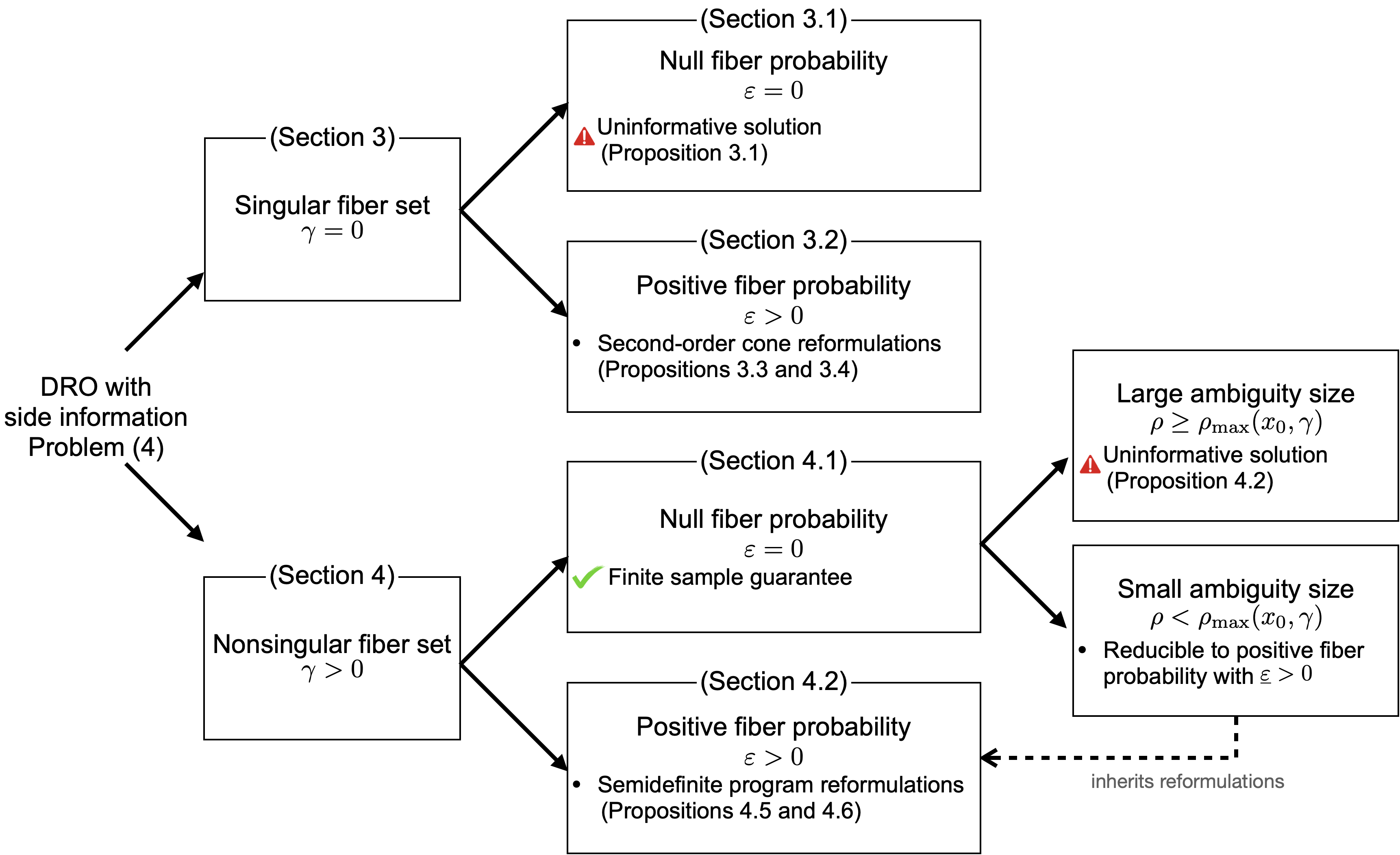
Figure 1. Schematic overview of the results in this paper.

The parameter $\gamma$ determines the size of the neighborhood around $x_{0}$. The case with $\gamma=0$ results in a singular fiber set $\{x_{0}\}\times\mathcal{Y}$: in this case, either problem (4) leads to uninformative conditioning result in Section 3.1 or we need to impose a strictly positive mass in order to get informative conditioning result ($\varepsilon>0$) in Section 3.2. Notice that imposing the constraint that $\mathbb{Q}(X=x_{0})\geq\varepsilon>0$ will automatically eliminates distributions with a density around $x_{0}$. Thus, if the modeler has a prior belief that the data-generating distribution admits a density around $x_{0}$, then it is more reasonable to use $\gamma>0$. The parameter $\gamma$ prescribes a neighborhood in the covariate space $\mathcal{X}$, and it resembles the kernel bandwidth in the field of nonparametric statistics. One can rely on this resemblance and decide to tune $\gamma$ based on the number of samples $N$ using the same theoretical guidance for choosing the bandwidth. For example, if $\mathcal{X}$ is one-dimensional, then [36, Section 3.2] suggests that $\gamma$ should be of the order of $1/N^{1/5}$. For higher dimensions, the rate can be obtained by imposing suitable assumptions on the data generating distribution.

Adding a neighborhood around $x_{0}$ also implies that the modeler wishes to hedge against potential misspecification or perturbation of the covariate $x_{0}$. In a portfolio optimization setting, the covariate $x_{0}$ may represent a combination of macroeconomics (inflation, GDP growth, etc.) and/or market indices (VIX, etc.), which are notoriously difficult to assign an exact value due to time lags, noisy or constantly-updated measurements. It is thus imperative to take the effects of an uncertain covariate $x_{0}$ into account.

From a technical viewpoint, the parameter $\varepsilon$ helps to avoid the ill-posedness of the optimization problem. As we will show in Sections 3.1 and 4.1, the conditioning in problem (4) may become uninformative if $\varepsilon=0$, and this issue can be eliminated by imposing a strictly positive value of $\varepsilon$. From a modeling view point, the parameter $\varepsilon$ can capture the prior information of the modeler on the magnitude of the density function around $x_{0}$, which translates integrally to a lower-confidence bound on the probability value assigned to the set $\mathcal{N}_{\gamma}(x_{0})\times\mathcal{Y}$. Alternatively, the parameter $\varepsilon$ can be tuned using a similar idea as how one tunes the kernel bandwidth in the nonparametric statistics literature: if the neighborhood around $x_{0}$ is of a radius $\gamma>0$ and if the data-generating distribution admits a density, then we expect $\varepsilon$ to scale in the order of $\gamma^{n}$, where $n$ is the dimension of the covariate space $\mathcal{X}$.

Finally, the parameter $\rho\in\mathbb{R}_{++}$ hedges against possible error in the finite sample estimation, or equivalently known as the epistemic uncertainty. It is possible to tune $\rho$ so that problem (4) possesses some desirable theoretical guarantees. For example, under the condition $\gamma>0$ and $\varepsilon=0$ of Section 4.1, problem (4) satisfies the finite sample guarantee provided that $\rho$ is chosen so that $\mathbb{B}_{\rho}$ contains the data-generating distribution with high probability (e.g., by choosing $\rho$ that satisfies the finite guarantee from [39]). Alternatively, $\rho$ can be also tuned using the robust Wasserstein profile inference (RWPI) approach with the goal of recovering the correct decision [17, 75].

The most comprehensive and general case in this paper is presented in Section 4.2 with all parameters $(\rho,\gamma,\varepsilon)$ being non-zero. In addition, the results in Section 4.2 also provide the reformulations for a specific case with $\varepsilon=0$, see the dashed arrow. Thus, the combination of non-zero parameters $(\rho,\gamma,\varepsilon)$ presented in Section 4.2 is useful in two fronts: first, it equips the modeler with the most flexible setting to capture different prior information, and second, it serves as a reformulating auxiliary combination to resolve the problem under a null fiber probability assumption.

While the statistical performance guarantees (either in asymptotic or finite sample regime) of problem (4) is also of high theoretical relevance, our paper focuses mainly on the practical relevance. Towards this goal, our main focus is to provide the reformulations for problem (4) via a complete and thorough analysis for each combination of the parameters $(\rho,\gamma,\varepsilon)$. We leave the statistical performance guarantee of problem (4) open for further research.

3. Tractable Reformulations for Singular Fiber Set

We study in this section the case where the radius $\gamma$ is zero, which implies that $\mathcal{N}_{\gamma}(x_{0})=\{x_{0}\}$ and the fiber set becomes $\{x_{0}\}\times\mathcal{Y}$. In this case, we simply recover the conventional portfolio allocation problem conditional on $X=x_{0}$. Interestingly, the qualitative behavior of the robustified conditional portfolio allocation problem (4) depends on whether $\varepsilon=0$ or $\varepsilon>0$. We will explore these two cases in the subsequent subsections.

3.1. Null fiber probability $\varepsilon=0$

We consider now the situation when $\gamma=\varepsilon=0$. Notice that the probability mass constraint in this case should be taken as a strict inequality of the form $\mathbb{Q}(X=x_{0})>0$ to avoid conditioning on sets of measure zero. This is equivalent to viewing the mass constraint in the limit as $\varepsilon$ tends to zero. If we use the type-$\infty$ Wasserstein distance to dictate the set $\mathbb{B}_{\rho}$, then the results from [61] can be utilized in order the compute the worst-case conditional expected loss. However, in this paper, we use the optimal transport of Definition 2.1 to prescribe $\mathbb{B}_{\rho}$, and the worst-case expected loss becomes uninformative as is shown in the following result.

Proposition 3.1 (Uninformative solution when $\varepsilon=\gamma=0$).

Suppose that $\varepsilon=\gamma=0$. For any $x_{0}\in\mathcal{X}$ and $\rho\in\mathbb{R}_{++}$, the worst-case conditional expected loss becomes

$$\sup\limits_{\mathbb{Q}\in\mathbb{B}_{\rho},\mathbb{Q}(X=x_{0})>0}~{}\mathds{E}_{\mathbb{Q}}[\ell(Y,\alpha,\beta)|X=x_{0}]=\sup\limits_{y\in\mathcal{Y}}~{}\ell(y,\alpha,\beta).$$

The result in Proposition 3.1 can be justified heuristically as follows. Consider an adversary who can move sample points on $\mathcal{X}\times\mathcal{Y}$ to maximize the loss subject to the optimal transport distance budget constraint. If $\widehat{x}_{i}=x_{0}$, then the adversary can slightly perturb $\widehat{x}_{i}$ within a infinitesimal distance so that the sample no longer belongs to the fiber set. Because of Assumption 2.4 on the continuity of the ground metric and the non-emptiness of the neighborhood, this perturbation cost an infinitesimally small amount of energy. The adversary can repeat until there is no sample point lying on the fiber set. Now, the adversary can pick any sample and slice out a tiny amount of mass and move that slice to any location on $\{x_{0}\}\times\mathcal{Y}$. Because the ground metric is continuous by Assumption 2.4(i) and because the slice can be chosen arbitrarily small, this would cost an infinitesimally small amount of energy. As the thin slice can be put on any point on $\{x_{0}\}\times\mathcal{Y}$, the resulting distribution will generate the robust conditional expected loss.

Proposition 3.1 reveals that the conditioning problem with $\varepsilon=\gamma=0$ results in a robust optimization formulation, which can be overly conservative. This result is also negative in the sense that the worst-case conditional expected loss depends only on the support $\mathcal{Y}$, and it does not depend on the data $(\widehat{x}_{i},\widehat{y}_{i})$ that were collected. Thus, in this case, the notion of data-driven decision-making becomes obsolete, and thus we do not pursue the reformulation any further. These observations also highlight the qualitative difference between using the optimal transport ambiguity set $\mathbb{B}_{\rho}$ as in this paper and using the $\infty$-Wasserstein ambiguity set as in [61, §2].

3.2. Strictly positive fiber probability $\varepsilon>0$

We now study the situation with a singular fiber set prescribed by $\gamma=0$, but the probability mass requirement is set to a strict positive value $\varepsilon\in(0,1]$. The robust conditional portfolio allocation problem (4) can now be rewritten explicitly as

$$\min\limits_{\alpha\in\mathcal{A},~{}\beta\in\mathcal{B}}~{}\sup\limits_{\mathbb{Q}\in\mathbb{B}_{\rho},\mathbb{Q}(X=x_{0})\geq\varepsilon}~{}\mathds{E}_{\mathbb{Q}}[\ell(Y,\alpha,\beta)|X=x_{0}].$$ (10)

The next theorem asserts that the worst-case conditional expected loss admits a finite-dimensional reformulation.

Theorem 3.2 (Worst-case conditional expected loss when $\gamma=0$).

Suppose that $\varepsilon\in(0,1]$ and $\rho>\rho_{\min}(x_{0},0,\varepsilon)$. For any feasible solution $(\alpha,\beta)$, we have

$$\sup\limits_{\mathbb{Q}\in\mathbb{B}_{\rho},\mathbb{Q}(X=x_{0})\geq\varepsilon}~{}\mathds{E}_{\mathbb{Q}}[\ell(Y,\alpha,\beta)|X=x_{0}]$$

$$= \inf\limits_{\begin{subarray}{c}\lambda_{1}\in\mathbb{R}_{+}\\ \lambda_{2}\in\mathbb{R}\end{subarray}}\left\{\rho\lambda_{1}+\varepsilon\lambda_{2}+\frac{1}{N}\sum_{i\in[N]}\left(\sup_{y_{i}\in\mathcal{Y}}\big{\{}\varepsilon^{-1}\ell(y_{i},\alpha,\beta)-[\mathbb{D}_{\mathcal{X}}(x_{0},\widehat{x}_{i})+\mathbb{D}_{\mathcal{Y}}(y_{i},\widehat{y}_{i})]\lambda_{1}-\lambda_{2}\big{\}}\right)^{+}\right\}.$$

It is instructive to discuss the insights that lead to the result presented in Theorem 3.2. Notice that the supremum problem in the statement of Theorem 3.2 has a fractional objective function. The first step of the proof establishes that without any loss of optimality, the inequality constraint $\mathbb{Q}(X=x_{0})\geq\varepsilon$ can be reduced to an equality constraint of the form $\mathbb{Q}(X=x_{0})=\varepsilon$ (see Proposition A.5 for a formal statement of this result). Leveraging this result, we derive the equivalence

$$\sup\limits_{\mathbb{Q}\in\mathbb{B}_{\rho},\mathbb{Q}(X=x_{0})\geq\varepsilon}~{}\mathds{E}_{\mathbb{Q}}[\ell(Y,\alpha,\beta)|X=x_{0}]=\sup\limits_{\mathbb{Q}\in\mathbb{B}_{\rho},\mathbb{Q}(X=x_{0})=\varepsilon}~{}\frac{1}{\varepsilon}\mathds{E}_{\mathbb{Q}}[\ell(Y,\alpha,\beta)\mathbbm{1}_{\{x_{0}\}}(X)],$$

where the right-hand side problem is linear in the probability measure $\mathbb{Q}$. At this point, duality techniques can be applied to reformulate the original problem into a finite-dimensional optimization problem.

We acknowledge that a similar duality result has been proposed in [32, Theorem 1] using the trimming approach. Notice that the trimming procedure in [32] is rather restrictive: it was designed so that any feasible distribution $\mathbb{Q}$ should satisfy $\mathbb{Q}(X=x_{0})=\varepsilon$, and thus the fractional objective function becomes a linear function of $\mathbb{Q}$. In direct comparison, our approach can be considered to be less stringent: we only impose an inequality $\mathbb{Q}(X=x_{0})\geq\varepsilon$, and thus our adversary has a bigger feasible set and is more powerful.

By combining the infimum reformulation of Theorem 3.2 with the outer infimum problem of problem (10), the portfolio allocation problem (10) is thus reformulatable as a finite-dimensional optimization problem. More specifically, problem (10) becomes

$$\begin{array}[]{cll}\inf&\displaystyle\rho\lambda_{1}+\varepsilon\lambda_{2}+\frac{1}{N}\sum_{i\in[N]}\theta_{i}\\ \operatorname{s.t.}&\alpha\in\mathcal{A},\;\beta\in\mathcal{B},\;\lambda_{1}\in\mathbb{R}_{+},\;\lambda_{2}\in\mathbb{R},\;\theta\in\mathbb{R}_{+}^{N}\\ &\theta_{i}\geq\sup_{y_{i}\in\mathcal{Y}}\big{\{}\varepsilon^{-1}\ell(y_{i},\alpha,\beta)-\mathbb{D}_{\mathcal{Y}}(y_{i},\widehat{y}_{i})\lambda_{1}\big{\}}-\mathbb{D}_{\mathcal{X}}(x_{0},\widehat{x}_{i})\lambda_{1}-\lambda_{2}\quad\forall i\in[N].\end{array}$$ (11)

In Propositions 3.3 and 3.4, we provide a second-order cone reformulation of problem (11) tailored for the mean-variance and mean-CVaR objective functions for a special instance with $\mathcal{X}=\mathbb{R}^{n}$, $\mathcal{Y}=\mathbb{R}^{m}$, $\mathbb{D}_{\mathcal{X}}(x,\widehat{x})=\|x-\widehat{x}\|^{2}$ and $\mathbb{D}_{\mathcal{Y}}(y,\widehat{y})=\|y-\widehat{y}\|_{2}^{2}$. Notice that $\mathbb{D}_{\mathcal{X}}$ is constructed from an arbitrary norm on $\mathbb{R}^{n}$ while $\mathbb{D}_{\mathcal{Y}}$ is constructed as the squared Euclidean norm on $\mathbb{R}^{m}$.

Proposition 3.3 (Mean-variance loss function).

Suppose that $\ell$ is the mean-variance loss function of the form (5), $\gamma=0$, $\varepsilon\in(0,1]$ and $\rho>\rho_{\min}(x_{0},0,\varepsilon)$. Suppose in addition that $\mathcal{X}=\mathbb{R}^{n},\mathcal{Y}=\mathbb{R}^{m}$, $\mathbb{D}_{\mathcal{X}}(x,\widehat{x})=\|x-\widehat{x}\|^{2}$ and $\mathbb{D}_{\mathcal{Y}}(y,\widehat{y})=\|y-\widehat{y}\|_{2}^{2}$. The distributionally robust portfolio allocation model with side information (10) is equivalent to the second-order cone program

$$\begin{array}[]{cll}\inf&\displaystyle\rho\lambda_{1}+\varepsilon\lambda_{2}+\frac{1}{N}\sum_{i\in[N]}\theta_{i}\\ \operatorname{s.t.}&\alpha\in\mathcal{A},\;\beta\in\mathcal{B},\;\lambda_{1}\in\mathbb{R}_{+},\;\lambda_{2}\in\mathbb{R},\;\theta\in\mathbb{R}_{+}^{N},\;z\in\mathbb{R}_{+}^{N},\;w\in\mathbb{R}\\ &0\leq w\leq 1,\quad\left\|\begin{bmatrix}2\alpha\\ 1-w-\varepsilon\lambda_{1}\end{bmatrix}\right\|_{2}\leq 1-w+\varepsilon\lambda_{1}\\ &z_{i}=\varepsilon\theta_{i}+\varepsilon\|x_{0}-\widehat{x}_{i}\|^{2}\lambda_{1}+\varepsilon\lambda_{2}+\frac{1}{4}\eta^{2}+\eta\beta,\quad\left\|\begin{bmatrix}2\,\widehat{y}_{i}^{\top}\alpha-2\beta-\eta\\ z_{i}-w\end{bmatrix}\right\|_{2}\leq z_{i}+w&\forall i\in[N].\end{array}$$

Proposition 3.4 (Mean-CVaR loss function).

Suppose that $\ell$ is the mean-CVaR loss function of the form (6), $\gamma=0$, $\varepsilon\in(0,1]$ and $\rho>\rho_{\min}(x_{0},0,\varepsilon)$. Suppose in addition that $\mathcal{X}=\mathbb{R}^{n}$, $\mathcal{Y}=\mathbb{R}^{m}$, $\mathbb{D}_{\mathcal{X}}(x,\widehat{x})=\|x-\widehat{x}\|^{2}$ and $\mathbb{D}_{\mathcal{Y}}(y,\widehat{y})=\|y-\widehat{y}\|_{2}^{2}$. The distributionally robust portfolio allocation model with side information (10) is equivalent to the second-order cone program

$$\begin{array}[]{cll}\inf&\displaystyle\rho\lambda_{1}+\varepsilon\lambda_{2}+\frac{1}{N}\sum_{i\in[N]}\theta_{i}\\ \operatorname{s.t.}&\alpha\in\mathcal{A},\;\beta\in\mathcal{B},\;\lambda_{1}\in\mathbb{R}_{+},\;\lambda_{2}\in\mathbb{R},\;\theta\in\mathbb{R}_{+}^{N},\;z\in\mathbb{R}_{+}^{N},\;\tilde{z}\in\mathbb{R}_{+}^{N}\\ &\left.\!\!\!\begin{array}[]{l}z_{i}=\theta_{i}+\lambda_{1}\|x_{0}-\widehat{x}_{i}\|^{2}+\lambda_{2}+\varepsilon^{-1}\eta\widehat{y}_{i}^{\top}\alpha-\varepsilon^{-1}\beta\\ \tilde{z}_{i}=\theta_{i}+\lambda_{1}\|x_{0}-\widehat{x}_{i}\|^{2}+\lambda_{2}+\varepsilon^{-1}(\eta+\frac{1}{\tau})\widehat{y}_{i}^{\top}\alpha-\varepsilon^{-1}(1-\frac{1}{\tau})\beta\\ \left\|\begin{bmatrix}\varepsilon^{-1}\eta\alpha\\ z_{i}-\lambda_{1}\end{bmatrix}\right\|_{2}\leq z_{i}+\lambda_{1},\quad\left\|\begin{bmatrix}\varepsilon^{-1}(\eta+\tau^{-1})\alpha\\ \tilde{z}_{i}-\lambda_{1}\end{bmatrix}\right\|_{2}\leq\tilde{z}_{i}+\lambda_{1}\end{array}\right\}\forall i\in[N].\end{array}$$

Both Proposition 3.3 and 3.4 leverage the fact that $\mathcal{Y}=\mathbb{R}^{m}$ in order to simplify the semi-infinite constraints into second-order cone constraints. We re-emphasize that under the assumption $\mathcal{Y}=\mathbb{R}^{m}$ of Proposition 3.3 and 3.4, formulation (10) is a conservative approximation of the distributionally robust mean-variance and mean-CVaR portfolio allocation problem, respectively. In case the set $\mathcal{Y}$ is an ellipsoid of the form $\mathcal{Y}=\{y\in\mathbb{R}^{m}:y^{\top}Qy+2q^{\top}y+q_{0}\leq 0\}$ with a non-empty interior, then semi-definite cone constraint counterparts are also available by employing the S-lemma [65].

4. Tractable Reformulations for Nonsingular Conditioning Set

We now focus on the portfolio allocation conditional on $X\in\mathcal{N}_{\gamma}(x_{0})$ for some radius $\gamma>0$. A fiber set of the form $\mathcal{N}_{\gamma}(x_{0})\times\mathcal{Y}$ was first used in [61] in the conditional estimation setting with the aim to hedge against noisy covariate information $x_{0}$ and also to improve the statistical performance of the solution approach. The results from [61] rely heavily from the specification of the ambiguity set using the type-$\infty$ Wasserstein distance, and these results are not transferrable to the ambiguity set under investigation in this paper. As a parallel counterpart to Section 3, we will study two separate cases depending on whether the probability requirement $\varepsilon$ is zero or strictly positive. We start by discussing the case when $\varepsilon=0$.

4.1. Null fiber probability $\varepsilon=0$

Similar to Section 3.1, we consider the probability mass constraint of the form $\mathbb{Q}(X\in\mathcal{N}_{\gamma}(x_{0}))>0$ with a strict inequality to avoid conditioning on sets of measure zero. Problem (4) becomes

$$\min\limits_{\alpha\in\mathcal{A},~{}\beta\in\mathcal{B}}~{}\sup\limits_{\mathbb{Q}\in\mathbb{B}_{\rho},\mathbb{Q}(X\in\mathcal{N}_{\gamma}(x_{0}))>0}~{}\mathds{E}_{\mathbb{Q}}[\ell(Y,\alpha,\beta)|X\in\mathcal{N}_{\gamma}(x_{0})].$$ (12)

Problem (12) is of particular interest thanks to its finite sample guarantee: if the samples are independently and identically distributed, and the radius $\rho$ is chosen judiciously, then the (unknown) data-generating distribution belongs to $\mathbb{B}_{\rho}$ with high probability. As such, the optimal value of problem (12) constitutes an upper bound on the worst-case conditional expected loss under the data-generating distribution. One possible way to choose $\rho$ to obtain the finite sample guarantee is by using the seminal result from [39].

The complication of conditioning on sets of measure zero, as highlighted in Section 3.1 for $\varepsilon=0$, still arises in this case when the radius $\rho$ is big enough. To illustrate this problem, we define the following quantity

$$\rho_{\max}(x_{0},\gamma)\triangleq\inf\left\{\mathds{W}(\mathbb{Q},\widehat{\mathbb{P}}):\mathbb{Q}\in\mathcal{M}(\mathcal{X}\times\mathcal{Y}),~{}\mathbb{Q}(X\in\mathcal{N}_{\gamma}(x_{0}))=0\right\}.$$

Intuitively, $\rho_{\max}(x_{0},\gamma)$ indicates the minimum budget required to transport all the training samples out of the fiber $\mathcal{N}_{\gamma}(x_{0})\times\mathcal{Y}$. If the empirical distribution $\widehat{\mathbb{P}}$ satisfies $\widehat{\mathbb{P}}(X\in\mathcal{N}_{\gamma}(x_{0}))=0$, which means that there is no training samples $(\widehat{x}_{i},\widehat{y}_{i})$ falling inside the fiber set $\mathcal{N}_{\gamma}(x_{0})\times\mathcal{Y}$, then it is trivial that $\rho_{\max}(x_{0},\gamma)=0$. If $\widehat{\mathbb{P}}(X\in\mathcal{N}_{\gamma}(x_{0}))>0$, then the value of $\rho_{\max}(x_{0},\gamma)$ is known in closed form. To this end, define the following index sets

$$\mathcal{I}_{1}=\{i\in[N]:\widehat{x}_{i}\in\mathcal{N}_{\gamma}(x_{0})\},\qquad\mathcal{I}_{2}=\{i\in[N]:\widehat{x}_{i}\not\in\mathcal{N}_{\gamma}(x_{0})\}.$$ (13)

The sets $\mathcal{I}_{1}$ and $\mathcal{I}_{2}$ divides the training samples into two mutually exclusive sets dependent on whether the training samples fall inside or outside the fiber. For any $i\in[N]$, let $d_{i}$ be the distance from $\widehat{x}_{i}$ to the boundary $\partial\mathcal{N}_{\gamma}(x_{0})$ of the set $\mathcal{N}_{\gamma}(x_{0})$, that is,

$$\forall i\in[N]:\qquad d_{i}=\min\limits_{x\in\partial\mathcal{N}_{\gamma}(x_{0})}\mathbb{D}_{\mathcal{X}}(x,\widehat{x}_{i}).$$ (14)

Note that the distance $d_{i}$ defined above is closely related to the values of $\kappa_{i}$ that is defined in (7). Indeed, if $\widehat{x}_{i}\not\in\mathcal{N}_{\gamma}(x_{0})$ then $d_{i}$ is equal to $\kappa_{i}$. However, if $\widehat{x}_{i}$ is in the interior of the set $\mathcal{N}_{\gamma}(x_{0})$ then $d_{i}>0$ while $\kappa_{i}=0$. Evaluating $d_{i}$ is, unfortunately, difficult in general because the set $\partial\mathcal{N}_{\gamma}(x_{0})$ may be non-convex. However, under certain choice of $\mathbb{D}_{\mathcal{X}}$, then $d_{i}$ can be computed efficiently. For example, when $\mathbb{D}_{\mathcal{X}}$ is the Euclidean norm, then it is easy to see that

$$d_{i}=\min\limits_{x:\|x-x_{0}\|_{2}=\gamma}~{}\|x-\widehat{x}_{i}\|_{2}=\gamma-\|x_{0}-\widehat{x}_{i}\|_{2}$$

for any $i\in\mathcal{I}_{1}$ implying that $\|x_{0}-\widehat{x}_{i}\|_{2}\leq\gamma$.

Using the definition of the set $\mathcal{I}_{1}$ and the boundary projection distance $d_{i}$, the maximum radius $\rho_{\max}(x_{0},\gamma)$ can be computed in closed form, as asserted by the next proposition.

Proposition 4.1 (Expression for $\rho_{\max}(x_{0},\gamma)$).

We have $\rho_{\max}(x_{0},\gamma)=N^{-1}\sum_{i\in\mathcal{I}_{1}}d_{i}$.

The result of Proposition 4.1 is also intuitive: if $\widehat{x}_{i}\in\mathcal{N}_{\gamma}(x_{0})$ then $i\in\mathcal{I}_{1}$, and we will need a sample-wise budget of $d_{i}/N$ to transport $(\widehat{x}_{i},\widehat{y}_{i})$ out of the fiber set $\mathcal{N}_{\gamma}(x_{0})\times\mathcal{Y}$. The value $\rho_{\max}(x_{0},\gamma)$ is thus obtained by summing all $d_{i}/N$ over the set $\mathcal{I}_{1}$. If $\mathcal{I}_{1}=\emptyset$ then there is no training sample inside the fiber set, and thus $\rho_{\max}(x_{0},\gamma)=0$. Proposition 4.1 also highlights that computing $\rho_{\max}(x_{0},\gamma)$ necessitates evaluating $|\mathcal{I}_{1}|$ values $d_{i}$ for each $i\in\mathcal{I}_{1}$.

The computation of $\rho_{\max}(x_{0},\gamma)$ provides a natural upper bound on the radius $\rho$. Indeed, if the radius $\rho$ prescribing the ambiguity set is bigger than $\rho_{\max}(x_{0},\gamma)$, then we recover the robust worst-case conditional loss. This robust loss is uninformative because it depends only on the support $\mathcal{Y}$ and it is independent of the training samples. This negative result is reminiscent of Proposition 4.2 and highlights once again the sophistication of the distributionally robust conditional decision-making problem.

Proposition 4.2 (Uninformative solution when $\rho$ is sufficiently large).

When $\gamma\in\mathbb{R}_{++}$, $\varepsilon=0$, and $\rho>\rho_{\max}(x_{0},\gamma)$, we have

$$\sup\limits_{\mathbb{Q}\in\mathbb{B}_{\rho},\mathbb{Q}(X\in\mathcal{N}_{\gamma}(x_{0}))>0}~{}\mathds{E}_{\mathbb{Q}}[\ell(Y,\alpha,\beta)|X\in\mathcal{N}_{\gamma}(x_{0})]=\sup\limits_{y\in\mathcal{Y}}~{}\ell(y,\alpha,\beta).$$

We now provide a heuristic justification for the result of Proposition 4.2. To form the worst-case distribution, the adversary first moves all the samples with index in $\mathcal{I}_{1}$ out of the fiber, and this would cost an amount of energy $\rho_{\max}(x_{0},\gamma)$. After that, the adversary can pick any sample, slice out an infinitesimally small amount of mass, and then move that slice to any point in the fiber $\mathcal{N}_{\gamma}(x_{0})\times\mathcal{Y}$. Because $\rho>\rho_{\max}(x_{0},\gamma)$ and because the ground metric is continuous, this new arrangement of the samples is feasible, and constitutes the worst-case distribution that maximizes the conditional expected loss.

Consider now the case in which the ambiguity size $\rho$ is strictly smaller than the maximum value $\rho_{\max}(x_{0},\gamma)$. It can be shown that in this situation, any distribution $\mathbb{Q}$ that is feasible in the supremum problem of (10) should satisfy $\mathbb{Q}(X\in\mathcal{N}_{\gamma}(x_{0}))\geq\underline{\varepsilon}$ for some strictly positive lower bound $\underline{\varepsilon}$. Further, this value $\underline{\varepsilon}$ can be quantified by solving a linear optimization problem.

Proposition 4.3 (Strictly positive probability requirement equivalence).

Suppose that $\gamma\in\mathbb{R}_{++}$, $\varepsilon=0$ and $\rho<\rho_{\max}(x_{0},\gamma)$. Then there exists an $\underline{\varepsilon}>0$, such that the distributionally robust portfolio allocation model with side information (10) is equivalent to

$$\min_{\alpha\in\mathcal{A},~{}\beta\in\mathcal{B}}\;\sup\limits_{\mathbb{Q}\in\mathbb{B}_{\rho},\mathbb{Q}(X\in\mathcal{N}_{\gamma}(x_{0}))\geq\underline{\varepsilon}}~{}\mathds{E}_{\mathbb{Q}}[\ell(Y,\alpha,\beta)|X\in\mathcal{N}_{\gamma}(x_{0})].$$

In particular, this equivalence holds for

$$\underline{\varepsilon}=\min\left\{\frac{1}{N}\sum_{i\in\mathcal{I}_{1}}p_{i}:p\in[0,1]^{N},~{}\frac{1}{N}\sum_{i\in\mathcal{I}_{1}}d_{i}(1-p_{i})\leq\rho\right\}.$$

The linear program that defines $\underline{\varepsilon}$ in Proposition 4.3 can be further shown to be a fractional knapsack problem, and it can be solved efficiently to optimality using a greedy heuristics [50, Proposition 17.1]. The conditions of Proposition 4.3 are satisfied only when $\rho_{\max}(x_{0},\gamma)>0$, which further implies that $\mathcal{I}_{1}\neq\emptyset$ and there exists at least one training sample in the fiber set $\mathcal{N}_{\gamma}(x_{0})\times\mathcal{Y}$. With a ambiguity size $\rho$ which is strictly smaller than $\rho_{\max}(x_{0},\gamma)$, it is not possible for the adversary to remove all the samples out of the fiber set $\mathcal{N}_{\gamma}(x_{0})\times\mathcal{Y}$. The lower bound value $\underline{\varepsilon}$ here represents the lowest possible amount of probability mass that is left on the fiber.

The result of Proposition 4.3 indicates that the portfolio allocation problem when $\rho<\rho_{\max}(x_{0},\gamma)$ can be obtained by solving the general problem with a strictly positive probability mass requirement. This general case is our subject of study in the next subsection.

4.2. Strictly positive fiber probability $\varepsilon>0$

We now consider the last, and also the most general, case with a nonsingular fiber set $\gamma>0$ and a strictly positive fiber probability $\varepsilon>0$. More specifically, we aim to solve the portfolio allocation of the form

$$\min\limits_{\alpha\in\mathcal{A},~{}\beta\in\mathcal{B}}~{}\sup\limits_{\mathbb{Q}\in\mathbb{B}_{\rho},\mathbb{Q}(X\in\mathcal{N}_{\gamma}(x_{0}))\geq\varepsilon}~{}\mathds{E}_{\mathbb{Q}}[\ell(Y,\alpha,\beta)|X\in\mathcal{N}_{\gamma}(x_{0})].$$ (15)

Notice that problem (15) is also relevant to the case with null probability requirement of Section 4.1 because problem (15) is equivalent to problem (12) when $\rho<\rho_{\max}(x_{0},\gamma)$ by choosing a proper value of $\varepsilon$ (cf. Proposition 4.3). As the first step towards solving (15), we define the following feasible set for the dual variables

$$\mathcal{V}\triangleq\left\{\begin{array}[]{ll}(\lambda,s,\nu^{+},\nu^{-},\phi,\varphi,\psi)\in\mathbb{R}_{+}^{N}\times\mathbb{R}^{N}\times\mathbb{R}_{+}\times\mathbb{R}_{+}\times\mathbb{R}\times\mathbb{R}_{+}\times\mathbb{R}_{+}^{N}\text{ such that: }\\ \phi-d_{i}\varphi+\psi_{i}-s_{i}\geq 0&\forall i\in\mathcal{I}_{1}\\ \phi+d_{i}\varphi+\psi_{i}-s_{i}\geq 0&\forall i\in\mathcal{I}_{2}\\ \nu^{+}-\nu^{-}+(\sum_{i\in\mathcal{I}_{1}}d_{i}-N\rho)\varphi-\sum_{i\in[N]}\psi_{i}\geq 0\\ \varphi-\lambda_{i}\geq 0&\forall i\in[N]\end{array}\right\}.$$ (16)

The next theorem presents the finite dimensional reformulation of the worst-case conditional expected loss.

Theorem 4.4 (Worst-case conditional expected loss for $\varepsilon>0$).

Suppose that $\gamma\in\mathbb{R}_{++}$, $\varepsilon\in\mathbb{R}_{++}$, and $\rho>\rho_{\min}(x_{0},\gamma,\varepsilon)$. Let the parameters $d_{i}$ be defined as in (14). For any feasible solution $(\alpha,\beta)$, we have

$$\sup\limits_{\mathbb{Q}\in\mathbb{B}_{\rho},\mathbb{Q}(X\in\mathcal{N}_{\gamma}(x_{0}))\geq\varepsilon}~{}\mathds{E}_{\mathbb{Q}}[\ell(Y,\alpha,\beta)|X\in\mathcal{N}_{\gamma}(x_{0})]=\left\{\begin{array}[]{cll}\inf&\phi+(N\varepsilon)^{-1}\nu^{+}-N^{-1}\nu^{-}\\ \operatorname{s.t.}&(\lambda,s,\nu^{+},\nu^{-},\phi,\varphi,\psi)\in\mathcal{V}\\ &s_{i}\geq\sup\limits_{y_{i}\in\mathcal{Y}}~{}\{\ell(y_{i},\alpha,\beta)-\lambda_{i}\mathbb{D}_{\mathcal{Y}}(y_{i},\widehat{y}_{i})\}&\forall i\in[N].\end{array}\right.$$

We can join the minimization operator over $(\alpha,\beta)$ to the result of Theorem 4.4, and the portfolio allocation problem with side information (15) is equivalent to the following finite-dimensional optimization problem

$$\begin{array}[]{cll}\min&\phi+(N\varepsilon)^{-1}\nu^{+}-N^{-1}\nu^{-}\\ \operatorname{s.t.}&\alpha\in\mathcal{A},~{}\beta\in\mathcal{B},~{}(\lambda,s,\nu^{+},\nu^{-},\phi,\varphi,\psi)\in\mathcal{V}\\ &s_{i}\geq\sup\limits_{y_{i}\in\mathcal{Y}}~{}\{\ell(y_{i},\alpha,\beta)-\lambda_{i}\mathbb{D}_{\mathcal{Y}}(y_{i},\widehat{y}_{i})\}&\forall i\in[N].\end{array}$$ (17)

The last constraint of problem (17) is a semi-infinite constraint which can be reformulated into a set of semi-definite constraints under specific situations. These results are highlighted in Proposition 4.5 and 4.6.

Proposition 4.5 (Mean-variance loss function).

Suppose that $\ell$ is the mean-variance loss function of the form (5), $\gamma\in\mathbb{R}_{++}$, $\varepsilon\in(0,1]$ and $\rho>\rho_{\min}(x_{0},\gamma,\varepsilon)$. Suppose in addition that $\mathcal{Y}=\mathbb{R}^{m}$ and $\mathbb{D}_{\mathcal{Y}}(y,\widehat{y})=\|y-\widehat{y}\|_{2}^{2}$. Let the parameters $d_{i}$ be defined as in (14). The distributionally robust portfolio allocation model with side information (17) is equivalent to the semi-definite optimization problem

$$\begin{array}[]{cll}\min&\phi+(N\varepsilon)^{-1}\nu^{+}-N^{-1}\nu^{-}\\ \operatorname{s.t.}&\alpha\in\mathcal{A},~{}\beta\in\mathcal{B},~{}t\in\mathbb{R}_{+},~{}A_{i}\in\mathbb{S}_{+}^{m}\quad\forall i\in[N]\\ &(\lambda,s,\nu^{+},\nu^{-},\phi,\varphi,\psi)\in\mathcal{V}\\ &\begin{bmatrix}\lambda_{i}I-A_{i}&\alpha\\ \alpha^{\top}&1\end{bmatrix}\succeq 0,~{}\begin{bmatrix}A_{i}&(\beta+\eta/2)\alpha-\lambda_{i}\widehat{y}_{i}\\ (\beta+\eta/2)\alpha^{\top}-\lambda_{i}\widehat{y}_{i}^{\top}&s_{i}+\lambda_{i}\|\widehat{y}_{i}\|_{2}^{2}-t\end{bmatrix}\succeq 0&\forall i\in[N]\\ &\begin{bmatrix}t&\beta\\ \beta&1\end{bmatrix}\succeq 0.\end{array}$$

Proposition 4.6 (Mean-CVaR loss function).

Suppose that $\ell$ is the mean-CVaR loss function of the form (6), $\gamma\in\mathbb{R}_{++}$, $\varepsilon\in(0,1]$ and $\rho>\rho_{\min}(x_{0},\gamma,\varepsilon)$. Suppose in addition that $\mathcal{Y}=\mathbb{R}^{m}$ and $\mathbb{D}_{\mathcal{Y}}(y,\widehat{y})=\|y-\widehat{y}\|_{2}^{2}$. Let the parameters $d_{i}$ be defined as in (14). The distributionally robust portfolio allocation model with side information (17) is equivalent to the semi-definite optimization problem

$$\begin{array}[]{cll}\min&\phi+(N\varepsilon)^{-1}\nu^{+}-N^{-1}\nu^{-}\\ \operatorname{s.t.}&\alpha\in\mathcal{A},~{}\beta\in\mathcal{B},~{}(\lambda,s,\nu^{+},\nu^{-},\phi,\varphi,\psi)\in\mathcal{V}\\ &\begin{bmatrix}\lambda_{i}I&\frac{\eta}{2}\alpha-\lambda_{i}\widehat{y}_{i}\\ \frac{\eta}{2}\alpha^{\top}-\lambda_{i}\widehat{y}_{i}^{\top}&s_{i}+\lambda_{i}\|\widehat{y}_{i}\|_{2}^{2}-\beta\end{bmatrix}\succeq 0,~{}\begin{bmatrix}\lambda_{i}I&\frac{\eta\tau+1}{2\tau}\alpha-\lambda_{i}\widehat{y}_{i}\\ \frac{\tau+1}{2\tau}\alpha^{\top}-\lambda_{i}\widehat{y}_{i}^{\top}&s_{i}+\lambda_{i}\|\widehat{y}_{i}\|_{2}^{2}-(1-1/\tau)\beta\end{bmatrix}\succeq 0&\forall i\in[N].\end{array}$$

Both Proposition 4.5 and 4.6 leverage the fact that $\mathcal{Y}=\mathbb{R}^{m}$ in order to reformulate the problem using semi-definite constraint. Again, under the assumption $\mathcal{Y}=\mathbb{R}^{m}$, the reformulation (17) is a conservative approximation of the distributionally robust conditional portfolio allocation problem, thus the reformulations in Proposition 4.5 and 4.6 are also conservative approximations of the distributionally robust conditional mean-variance and mean-CVaR portfolio allocation problems, respectively. In case that $\mathcal{Y}$ is an ellipsoid with a non-empty interior of the form $\mathcal{Y}=\{y\in\mathbb{R}^{m}:y^{\top}Qy+2q^{\top}y+q_{0}\leq 0\}$ for some symmetric matrix $Q$, then the S-lemma [65] can also be applied to devise a similar semi-definite optimization problem, the details can be found in Appendix B.

Despite having a fractional objective function, the results in this section assert that distributionally robust portfolio allocation with side information problem can be solved efficiently using convex conic programming solvers. This is in stark contrast with existing results in distributionally robust fractional programming where only nonconvex reformulations are available, and the optimal solution is obtained by solving a sequence of convex optimization problems after bisection [44, 83].

5. Numerical Experiment

In this section, we compare the empirical performance of our proposed conditional portfolio allocation model against several benchmark models. To this end, we conduct the numerical experiment using real historical data collected from the US stock market. We describe the details of stock future return data and side informations as follows.

Return: We study the historical S&P500 constituents data from January 01, 2015 to January 01, 2021. At day $t$, the response variable $Y$ is defined as the 1-day stock percentage return from day $t$ to day $t+1$. The sampling frequency is one sample per day.

Side information: We employ the Fama-French three-factor model [34] to construct the covariate $X=(X_{1},X_{2},X_{3})\in\mathbb{R}^{3}$. Recall that the Fama-French three-factor model includes the market (Rm-Rf) factor, the “small minus big” (SMB) factor, and the “high minus low” (HML) factor. Each factor is defined as the 1-day return of an associated portfolio:

• Rm-Rf factor: the portfolio weight on each stock is proportional to its market capitalization (MC);

• SMB factor: longs the stocks with MC in the lowest 50% quantile and shorts the stocks with MC in the highest 50% quantile;

• HML factor: longs the stocks with P/E ratio in the highest 30% quantile and shorts the stocks with P/E ratio in the lowest 30% quantile.

At day $t$, let $X_{i,\text{raw}},i=1,2,3$ denote the 1-day factor return of Rm-Rf, SMB and HML respectively, from day $t$ to day $t+1$. The value of $X_{i,\text{raw}}$ can not be directly used in the portfolio optimization for day $t$ as it contains future information, therefore we construct synthetic factor return predictors $X_{i},i=1,2,3$ as the linear combination of $X_{i,\text{raw}}$ and Gaussian noise. The magnitude of the Gaussian noise is chosen such that the correlation between $X_{i,\text{raw}}$ and $X_{i}$ is $0.1$.

Models: We first determine the feasible region of the portfolio optimization problem. If a stock in the sampled stock pool is not tradable at day $t$, then we impose its weight to be zero. In addition, we prohibit short selling so we enforce the investment weight vector $\alpha$ to be non-negative. To summarize, we set the feasible region of the stock weight to be a subset of the non-negative simplex

$$\mathcal{A}=\left\{\alpha\in\mathbb{R}_{+}^{m}\mid\sum_{i\in[m]}\alpha_{i}=1,~{}\alpha_{j}=0\mbox{ if stock }j\mbox{ is not tradable}\right\}.$$

In this section, we compare the empirical performance of several variations of the mean-variance models. The models to compare in this section include the original mean-variance model by Markowitz [56], the variation that exploits the side information, the variation that utilizes the distributionally robust framework, and the variations that leverage both elements (e.g., the model introduced in this paper). Please see below for a full list of models and their definitions.

1. the Equal Weighted model (EW): in this case, the portfolio allocation solves

   $$\min\limits_{\alpha\in\mathcal{A}}~{}\|\alpha\|_{2}.$$ (EW)

   If all stocks are tradable, then the EW allocation coincides with the $1/m$-portfolio, which is renowned for its robustness [26]. This portfolio is parameter-free, and was previously shown to be the limit of the distributionally robust portfolio allocations as the ambiguity size increases [63].

2. the unconditional Mean-Variance model (MV) [56]: the portfolio allocation solves

   $$\min\limits_{\alpha\in\mathcal{A},~{}\beta\in\mathbb{R}}\mathds{E}_{\widehat{\mathbb{P}}}[\ell(Y,\alpha,\beta)]$$ (MV)

   with the loss function $\ell$ prescribed in (5), and the distribution $\widehat{\mathbb{P}}$ is the empirical distribution supported on the available return data.

3. the Distributionally Robust unconditional Mean-Variance model (DRMV): the portfolio allocation solves

   $$\min\limits_{\alpha\in\mathcal{A}}~{}\sqrt{\alpha^{\top}\textrm{Variance}_{\widehat{\mathbb{P}}}(Y)\alpha}-\eta\cdot\alpha^{\top}\mathds{E}_{\widehat{\mathbb{P}}}[Y]+\sqrt{(1+\eta^{2})\rho}\|\alpha\|_{2}.$$ (DRMV)

   The above optimization problem is the reformulation of the distributionally robust mean-variance portfolio allocation with a Wasserstein ambiguity set on the distributions of the asset returns $Y$ [14]. The tuning parameter for this method is $\rho\in\{0.1,0.2,0.5\}$.

4. the Conditional Mean-Variance model (CMV): the portfolio allocation solves

   $$\min\limits_{\alpha\in\mathcal{A},~{}\beta\in\mathbb{R}}\mathds{E}_{\widehat{\mathbb{P}}}[\ell(Y,\alpha,\beta)|X\in\mathcal{N}_{\gamma}(x_{0})],$$ (CMV)

   where the loss function $\ell$ is prescribed in (5). The parameter $\gamma$ is set to the $a$-quantile of the empirical distribution of the distance between $x_{0}$ and the training covariate vectors, where the quantile value is in the range $a\in\{10\%,20\%,50\%\}$. Notice that by the choice of $\gamma$, the empirical distribution satisfies $\widehat{\mathbb{P}}(X\in\mathcal{N}_{\gamma}(x_{0}))>0$ and the conditional expectation is well-defined.

5. the Distributionally Robust Conditional Mean-Variance model (DRCMV) with type-$\infty$ Wasserstein ambiguity set [61], in which the portfolio allocation solves

   $$\min\limits_{\alpha\in\mathcal{A},~{}\beta\in\mathbb{R}}\sup\limits_{\mathbb{Q}\in\mathbb{B}^{\infty}_{\rho},\mathbb{Q}(X\in\mathcal{N}_{\gamma}(x_{0}))>0}~{}\mathds{E}_{\mathbb{Q}}[\ell(Y,\alpha,\beta)|X\in\mathcal{N}_{\gamma}(x_{0})].$$ (DRCMV)

   The parameter $\gamma$ is set to the $a$-quantile of the empirical distribution of the distance between $x_{0}$ and the training covariate vectors, where the quantile value is in the range $\{10\%,20\%,50\%\}$. The radius $\rho$ is set to the $b$-quantile of the empirical distribution of the distance between $x_{0}$ and the training covariate vectors, where the quantile value is in the range $b\in\{5\%,10\%,25\%\}$. Using the result from [61, Proposition 2.5], this model can be reformulated as a second-order cone program (see Appendix C for definition of $\mathbb{B}_{\rho}^{\infty}$ and detailed derivation of the reformulation).

6. the Optimal Transport based (distributionally robust) Conditional Mean-Variance model (OTCMV) where the portfolio allocation is the solution to problem (10) with the mean-variance loss function (5)

   $$\min\limits_{\alpha\in\mathcal{A},~{}\beta\in\mathbb{R}}\sup\limits_{\mathbb{Q}\in\mathbb{B}_{\rho},\mathbb{Q}(X=x_{0})\geq\varepsilon}~{}\mathds{E}_{\mathbb{Q}}[\ell(Y,\alpha,\beta)|X=x_{0}].$$ (OTCMV)

   The tuning parameters for this model includes the probability bound $\varepsilon\in\{0.1,0.2,0.5\}$ and the radius $\rho=a\times\rho_{\min}$, where $a\in\{1.1,1.2,1.5\}$ and $\rho_{\min}$ denotes the minimum distance between the training covariate $(\widehat{x}_{i})_{i=1}^{N}$ and $x_{0}$. This model is equivalent to a second-order cone program thanks to Proposition 3.3.

Notice that the feasible set $\mathcal{B}$ is set to $\mathbb{R}$ in all methods. The ground costs are chosen with $\mathbb{D}_{\mathcal{X}}(x,\widehat{x})=\|x-\widehat{x}\|_{2}^{2}$ and $\mathbb{D}_{\mathcal{Y}}(y,\widehat{y})=\|y-\widehat{y}\|_{2}^{2}$. All models can be solved using the MOSEK quadratic program solver [58].

Experiments: We carry out 256 independent replications to ensure that the performance comparison is statistically significant. In each replication, we randomly sample $m=20$ stocks from the data set to be used as a stock pool. The training procedure is carried out as follows. At each trading day $t$, we apply different portfolio optimization models to construct portfolio of the stock pool, using the historical observation of $(X,Y)$ in the past $2$-year window to form the nominal distribution $\widehat{\mathbb{P}}$ (more precisely, we use $252\times 2$ observations precedent to $t$). Moreover, the covariate $x_{0}$ is chosen as the observation of $X$ at time $t$. To obtain the validation score, we compute the return for each time $t$ in the period between January 1, 2017 and December 31, 2018, and then calculate the realized Sharpe ratio as the validation score. We first tune the parameter $\eta$ of the loss function $\ell$ by choosing the MV model (EW) with $\eta\in[10^{-1},2\cdot 10^{1}]$ with 7 equidistant points in the logscale to maximize the validation score of the MV model. This selected $\eta$ is reused in all models: MV, DRMV, CMV, DRCMV and OTCMV. Subsequently, we tune the corresponding parameters for DRMV, CMV, DRCMV and OTCMV by selecting the hyper-parameters that maximize the validation score.

Test Results: To obtain the out-of-sample performance, we deploy the tuned model in a rolling horizon scheme on the testing data from January 1, 2019 to December 31, 2020. We report the experimental results of different models using the Sharpe ratios of the realized returns, which are usually used to compare the performance of different trading strategies. For each sampled experiment and a given portfolio optimization model, we denote the daily percentage return of the model by $r_{i}$ for $i\in[T]$, where $T$ is the total number of trading days in the test period. The annualized Sharpe ratio is computed using the following formula:

$$\mbox{annualized Sharpe ratio}\triangleq\sqrt{252}\times\left(\widehat{\mbox{mean}}(\{r_{i}\}_{i\in[T]})\Big{/}\widehat{\mbox{std}}(\{r_{i}\}_{i\in[T]})\right),$$

where $\widehat{\mbox{mean}}$ and $\widehat{\mbox{std}}$ denote the empirical mean and standard deviation estimator, respectively. Thus, for each model we compute 256 annualized Sharpe ratios obtained from the 256 independent experiments. In addition to the Sharpe ratio, we also report the following metrics:

• maximum drawdown (maxDraw): the maximum observed loss from a peak to a trough of a portfolio, before a new peak is attained;

• trade volume (tradeVol): the average trading volume per annum.

We present the validation results for each model corresponding to the optimal hyper-parameter in Table 1. Using the selected hyper-parameters ($a=1.1$ and $\varepsilon=0.1$), the OTCMV model achieves the largest Sharpe ratio and smallest maximum drawdown during the validation period. The performance of different models during the test period is presented in Table 2. The OTCMV model outperforms the rest of the mean-variance type of models in terms of mean return and Sharpe ratio, but its performance is worse than EW. However, it is noteworthy that the performance of the EW model is significantly different between validation period and test period: the mean return of the EW portfolio is low in the validation period, but is high in the test period. This observation suggests that the comparison between EW and other mean-variance models may not be stable across different time period. From Table 2, we also observe that the EW method suffers a high value of maximum drawdown (maxDraw), implying that an EW portfolio may suffer significant loss in a trough downturn. The trade volume in Table 2 also indicates that conditional portfolio allocations (CMV, DRCMV and OTCMV) trade more than unconditional allocations (EW, MV, DRMV). However, it is also important to note that among conditional portfolios, the robust portfolios have lower trade volume, and the OTCMV portfolio has the smallest trade volume among the three.

model	mean	stdDev	sharpe	maxDraw	tradeVol
EW	0.093	0.160	0.580	0.268	0.011
MV	0.107	0.137	0.777	0.187	0.032
DRMV	0.096	0.132	0.722	0.190	0.020
CMV	0.119	0.147	0.812	0.195	1.295
DRCMV	0.108	0.143	0.754	0.197	0.719
OTCMV	0.113	0.139	0.815	0.183	0.694

Table 1. Summary of portfolio performance during the validation period (from January 1, 2017 to December 31, 2018). For each model, we compare the performance corresponding to the best hyperparameter that leads to the largest Sharpe ratio.

model	mean	stdDev	sharpe	maxDraw	tradeVol
EW	0.266	0.322	0.828	0.533	0.015
MV	0.176	0.267	0.659	0.463	0.030
DRMV	0.178	0.265	0.670	0.476	0.023
CMV	0.178	0.291	0.612	0.485	1.353
DRCMV	0.169	0.273	0.621	0.488	0.748
OTCMV	0.215	0.275	0.782	0.463	0.667

Table 2. Summary of portfolio performance during test period (from January 1, 2019 to December 31, 2020).

In Figure 2, we present the histograms of the realized Sharpe ratio from 256 experiments during test period among three benchmarks: CMV, DRMV and OTCMV. The left-hand side plot compares the performance of OTCMV against that of DRMV, which reveals that integrating the contextual information into the distributionally robust optimization problem leads to higher average Sharpe ratio values. The right-hand side plot compares the performance of OTCMV against that of CMV, which demonstrates that distributional robustness reduces the occurrence of small realized Sharpe ratio values.

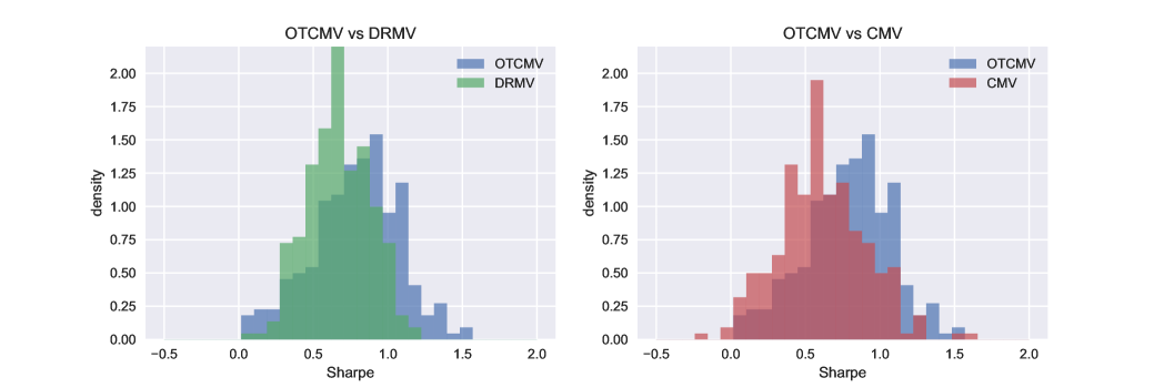
Figure 2. Histogram of realized Sharpe ratio values for competing mean-variance models. The realized Sharpe ratio values are computed using the test period data from January 1, 2019 to December 31, 2020.

In Figure 3, we compare the histogram of the daily returns between EW and OTCMV on the test dataset from January 1, 2019 to December 31, 2020, in order to demonstrate that OTCMV is more robust in the sense that its portfolio returns suffer from fewer and of lower-magnitude extreme one-day loss. We focus on the left tail of the daily return distributions to compare the downside risk. We observe from the histogram that EW suffers from more occurrences of single day loss exceeding 10% than OTCMV.

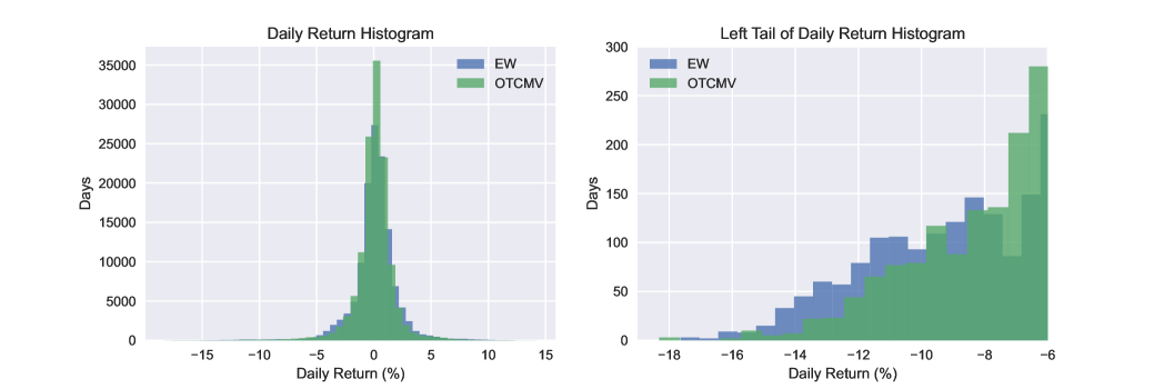
Figure 3. Histogram of the daily returns for EW vs OTCMV. The daily return is computed using the test period data from January 1, 2019 to December 31, 2020, thus each model contains $256\times 2$ years of data. The full histogram of daily return is presented in the left-hand side plot, while the right-hand side plot shows the left tails (return smaller than 6%) in magnification.

To gain further confirmation, we test whether the annualized Sharpe ratios of OTCMV are larger than that of the competing models by conducting a series of pairwise Wilcoxon signed-rank test [81]. It is important to note that the Wilcoxon signed-rank test does not assume the samples to be normally distributed. Against each competing method, we form the null and the alternative hypotheses of the Wilcoxon signed-rank test as follows:

• $\mathcal{H}_{\text{null}}$: With probability at least 1/2, the Sharpe ratio of OTCMV is smaller.

• $\mathcal{H}_{\text{alt}}$: With probability at least 1/2, the Sharpe ratio of OTCMV is larger.

The $p$-values for the tests are reported in Table 3. If we choose a significance level of 0.05, then the null hypothesis is rejected for all competing mean-variance type of models. The $p$-values for the test against EW is too large and the test fails to reject the null hypothesis in this case.

Model	EW	MV	DRMV	CMV	DRCMV
$p$-value	$0.997$	$<0.001$	$<0.001$	$<0.001$	$<0.001$

Table 3. $p$-values of the Wilcoxon signed-rank test during test period.

The numerical experiments in this paper largely focus on the mean-variance portfolio allocation problem. Additionally, we present a set of complete and independent results of the mean-CVaR models in Appendix D. Finally, we elaborate how our framework can be integrated into a contextual two-stage stochastic programming problem in Appendix E.

Acknowledgments.

Material in this paper is based upon work supported by the Air Force Office of Scientific Research under award number FA9550-20-1-0397. Additional support is gratefully acknowledged from NSF grants 1915967, 1820942, 1838676, NSERC grant RGPIN-2016-05208, and from the China Merchant Bank. Finally, this research was enabled in part by support provided by Compute Canada.

Appendix A Proofs of Main Results

A.1. Proofs of Section 2

The following results are needed to justify Lemmas 2.2 and 2.3.

Lemma A.1 (Interchange).

Suppose that $\mathcal{Y}$ and $\mathcal{B}$ are compact and that $\ell$ is continuous in $Y$ and convex in $\beta$. Then we have

$$\sup\limits_{\mathbb{Q}\in\mathbb{B}_{\rho},\mathbb{Q}(X\in\mathcal{N}_{\gamma}(x_{0}))\geq\varepsilon}\inf\limits_{\beta\in\mathcal{B}}~{}\mathds{E}_{\mathbb{Q}}[\ell(Y,\alpha,\beta)|X\in\mathcal{N}_{\gamma}(x_{0})]=\inf\limits_{\beta\in\mathcal{B}}\sup\limits_{\mathbb{Q}\in\mathbb{B}_{\rho},\mathbb{Q}(X\in\mathcal{N}_{\gamma}(x_{0}))\geq\varepsilon}~{}\mathds{E}_{\mathbb{Q}}[\ell(Y,\alpha,\beta)|X\in\mathcal{N}_{\gamma}(x_{0})].$$

A similar result on the interchange of the infimum and the supremum operators is obtained in [61, Lemma B.3]. Nevertheless, there is a subtle distinction on the conditions of the two results: Lemma A.1 requires that $\mathcal{Y}$ and $\mathcal{B}$ are compact, while [61, Lemma B.3] does not require these compactness conditions. This distinction emphasizes the qualitative difference between an $\infty$-Wasserstein ambiguity set of [61] and the optimal transport ambiguity set $\mathbb{B}_{\rho}$ in this paper. Indeed, the weak-compactness condition is automatically satisfied by the $\infty$-Wasserstein set in [61], but this condition is not satisfied by the set $\mathbb{B}_{\rho}$, which leads to the additional requirement on the compactness of $\mathcal{B}$ in Lemma A.1. Further, Lemma A.1 requires the compactness of $\mathcal{Y}$ for the upper-continuity of the objective function in $\mathbb{Q}$. On the contrary, the continuity condition is automatically satisfied by the $\infty$-Wasserstein set in [61].

The proof of Lemma A.1 follows from the convexity of the conditional ambiguity set. To this end, define the following ambiguity set

$$\mathcal{B}_{x_{0},\gamma,\varepsilon}(\mathbb{B}_{\rho})\triangleq\left\{\mu_{x_{0}}\in\mathcal{M}(\mathcal{Y}):\begin{array}[]{l}\exists\mathbb{Q}\in\mathbb{B}_{\rho}\text{ such that }\mathbb{Q}(\mathcal{N}_{\gamma}(x_{0})\times\mathcal{Y})\geq\varepsilon\\ ~{}\mathbb{Q}(\mathcal{N}_{\gamma}(x_{0})\times A)=\mu_{x_{0}}(A)\mathbb{Q}(\mathcal{N}_{\gamma}(x_{0})\times\mathcal{Y})~{}~{}\forall A\subseteq\mathcal{Y}~{}\text{ measurable}\end{array}\right\}.$$

Lemma A.2 (Convexity of $\mathcal{B}_{x_{0},\varepsilon,\gamma}(\mathbb{B}_{\rho})$).

If $\mathbb{B}_{\rho}$ is convex, then the conditional ambiguity set $\mathcal{B}_{x_{0},\gamma,\varepsilon}(\mathbb{B}_{\rho})$ is also convex.

The proof of Lemma A.2 can be obtained by a minor modification of the proof for [61, Lemma B.5]. The proof is included here for completeness.

Proof of Lemma A.2.

Let $\mu_{0}^{0},~{}\mu_{0}^{1}\in\mathcal{B}_{x_{0},\gamma,\varepsilon}(\mathbb{B}_{\rho})$ be two arbitrary probability measures supported on $\mathcal{Y}$. Associated with each $\mu_{0}^{j}$, $j\in\{0,1\}$, is a corresponding joint measure $\mathbb{Q}^{j}\in\mathcal{M}(\mathcal{X}\times\mathcal{Y})$ such that

$$\mathbb{Q}^{j}(\mathcal{N}_{\gamma}(x_{0})\times\mathcal{Y})\geq\varepsilon\quad\text{and}\quad\displaystyle\frac{\mathbb{Q}^{j}(\mathcal{N}_{\gamma}(x_{0})\times A)}{\mathbb{Q}^{j}(\mathcal{N}_{\gamma}(x_{0})\times\mathcal{Y})}=\mu_{0}^{j}(A)\quad\forall A\subseteq\mathcal{Y}~{}\text{measurable}.$$

Select any $\lambda\in(0,1)$. We now show that $\mu_{0}^{\lambda}=\lambda\mu_{0}^{1}+(1-\lambda)\mu_{0}^{0}\in\mathcal{B}_{x_{0},\gamma,\varepsilon}(\mathbb{B}_{\rho})$. Indeed, consider the joint measure

$$\mathbb{Q}^{\lambda}=\theta\mathbb{Q}^{1}+(1-\theta)\mathbb{Q}^{0},$$

where $\theta$ is defined as

$$\theta=\frac{\lambda\mathbb{Q}^{0}(\mathcal{N}_{\gamma}(x_{0})\times\mathcal{Y})}{\lambda\mathbb{Q}^{0}(\mathcal{N}_{\gamma}(x_{0})\times\mathcal{Y})+(1-\lambda)\mathbb{Q}^{1}(\mathcal{N}_{\gamma}(x_{0})\times\mathcal{Y})}\in[0,1].$$

By definition, we have $\mathbb{Q}^{\lambda}(\mathcal{N}_{\gamma}(x_{0})\times\mathcal{Y})\geq\varepsilon$, and by the convexity of $\mathbb{B}_{\rho}$, we have $\mathbb{Q}^{\lambda}\in\mathbb{B}_{\rho}$. Moreover, for any set $A\subseteq\mathcal{Y}$ measurable, we find

$$\frac{\mathbb{Q}^{\lambda}(\mathcal{N}_{\gamma}(x_{0})\times A)}{\mathbb{Q}^{\lambda}(\mathcal{N}_{\gamma}(x_{0})\times\mathcal{Y})} =\frac{\theta\mathbb{Q}^{1}(\mathcal{N}_{\gamma}(x_{0})\times A)+(1-\theta)\mathbb{Q}^{0}(\mathcal{N}_{\gamma}(x_{0})\times A)}{\theta\mathbb{Q}^{1}(\mathcal{N}_{\gamma}(x_{0})\times\mathcal{Y})+(1-\theta)\mathbb{Q}^{0}(\mathcal{N}_{\gamma}(x_{0})\times\mathcal{Y})}$$

$$=\frac{\lambda\mathbb{Q}^{0}(\mathcal{N}_{\gamma}(x_{0})\times\mathcal{Y})\mathbb{Q}^{1}(\mathcal{N}_{\gamma}(x_{0})\times A)+(1-\lambda)\mathbb{Q}^{1}(\mathcal{N}_{\gamma}(x_{0})\times\mathcal{Y})\mathbb{Q}^{0}(\mathcal{N}_{\gamma}(x_{0})\times A)}{\mathbb{Q}^{0}(\mathcal{N}_{\gamma}(x_{0})\times\mathcal{Y})\mathbb{Q}^{1}(\mathcal{N}_{\gamma}(x_{0})\times\mathcal{Y})}$$

$$=\frac{\lambda\mathbb{Q}^{1}(\mathcal{N}_{\gamma}(x_{0})\times A)}{\mathbb{Q}^{1}(\mathcal{N}_{\gamma}(x_{0})\times\mathcal{Y})}+\frac{(1-\lambda)\mathbb{Q}^{0}(\mathcal{N}_{\gamma}(x_{0})\times A)}{\mathbb{Q}^{0}(\mathcal{N}_{\gamma}(x_{0})\times\mathcal{Y})}$$

$$=\lambda\mu_{0}^{1}(A)+(1-\lambda)\mu_{0}^{0}(A),$$

where the second equality holds thanks to the definition of $\theta$. This line of argument implies that $\mu_{0}^{\lambda}\in\mathcal{B}_{x_{0},\gamma,\varepsilon}(\mathbb{B}_{\rho})$, and further asserts the convexity of $\mathcal{B}_{x_{0},\gamma,\varepsilon}(\mathbb{B}_{\rho})$. ∎

We are now ready to prove Lemma A.1.

Proof of Lemma A.1.

By rewriting the conditional expectation using the conditional measure $\mu_{0}$, we have for any value of $\alpha$

$$\sup\limits_{\mathbb{Q}\in\mathbb{B}_{\rho},\mathbb{Q}(X\in\mathcal{N}_{\gamma}(x_{0}))\geq\varepsilon}\inf\limits_{\beta\in\mathcal{B}}~{}\mathds{E}_{\mathbb{Q}}[\ell(Y,\alpha,\beta)|X\in\mathcal{N}_{\gamma}(x_{0})]=\sup\limits_{\mu_{0}\in\mathcal{B}_{x_{0},\gamma,\varepsilon}(\mathbb{B}_{\rho})}~{}\inf\limits_{\beta\in\mathcal{B}}~{}\mathds{E}_{\mu_{0}}[\ell(Y,\alpha,\beta)].$$

The set $\mathcal{B}_{x_{0},\gamma,\varepsilon}(\mathbb{B}_{\rho})$ is convex by Lemma A.2. Moreover, because $\ell$ is continuous in $Y$, the mapping $\mu_{0}\mapsto\mathds{E}_{\mu_{0}}[\ell(Y,\alpha,\beta)]$ is upper semicontinuous in the weak topology thanks to the compactness of $\mathcal{Y}$. Finally, $\mathcal{B}$ is compact and $\ell$ is convex in $\beta$. The interchangeability of the supremum and the infimum operators is now a consequence of the Sion’s minimax theorem [76]. ∎

We are now ready to prove the results in Section 2.

Proof of Lemma 2.2.

It is well-known that

$$\mathrm{Variance}_{\mathbb{Q}}[Y^{\top}\alpha|X\in\mathcal{N}_{\gamma}(x_{0})]=\min\limits_{\beta\in\mathbb{R}}~{}\mathds{E}_{\mathbb{Q}}[(Y^{\top}\alpha-\beta)^{2}|X\in\mathcal{N}_{\gamma}(x_{0})]$$

for any probability measure $\mathbb{Q}\in\mathcal{M}(\mathcal{X}\times\mathcal{Y})$, where the optimal $\beta$ is the conditional mean of $Y^{\top}\alpha$ given $X\in\mathcal{N}_{\gamma}(x_{0})$ under $\mathbb{Q}$. When $\mathcal{A}$ and $\mathcal{Y}$ are compact, the random variable $Y^{\top}\alpha$ has bounded mean for any $\mathbb{Q}\in\mathbb{B}_{\rho}$. More precisely, we have

$$\mathds{E}_{\mathbb{Q}}[Y^{\top}\alpha|X\in\mathcal{N}_{\gamma}(x_{0})]\in\mathcal{B},$$

where $\mathcal{B}$ is defined as in the statement of the lemma. Therefore, it is without any loss of optimality to restrict $\beta\in\mathcal{B}$. We thus find

$$\min\limits_{\alpha\in\mathcal{A}}~{}\sup\limits_{\mathbb{Q}\in\mathbb{B}_{\rho},\mathbb{Q}(X\in\mathcal{N}_{\gamma}(x_{0}))\geq\varepsilon}~{}\mathrm{Variance}_{\mathbb{Q}}[Y^{\top}\alpha|X\in\mathcal{N}_{\gamma}(x_{0})]-\eta\cdot\mathds{E}_{\mathbb{Q}}[Y^{\top}\alpha|X\in\mathcal{N}_{\gamma}(x_{0})]$$

$$= \min\limits_{\alpha\in\mathcal{A}}~{}\sup\limits_{\mathbb{Q}\in\mathbb{B}_{\rho},\mathbb{Q}(X\in\mathcal{N}_{\gamma}(x_{0}))\geq\varepsilon}~{}\min_{\beta\in\mathbb{R}}~{}\mathds{E}_{\mathbb{Q}}[\ell(Y,\alpha,\beta)|X\in\mathcal{N}_{\gamma}(x_{0})]$$

$$= \min\limits_{\alpha\in\mathcal{A}}~{}\sup\limits_{\mathbb{Q}\in\mathbb{B}_{\rho},\mathbb{Q}(X\in\mathcal{N}_{\gamma}(x_{0}))\geq\varepsilon}~{}\min_{\beta\in\mathcal{B}}~{}\mathds{E}_{\mathbb{Q}}[\ell(Y,\alpha,\beta)|X\in\mathcal{N}_{\gamma}(x_{0})]$$

$$= \min\limits_{\alpha\in\mathcal{A}}~{}\min_{\beta\in\mathcal{B}}~{}\sup\limits_{\mathbb{Q}\in\mathbb{B}_{\rho},\mathbb{Q}(X\in\mathcal{N}_{\gamma}(x_{0}))\geq\varepsilon}~{}\mathds{E}_{\mathbb{Q}}[\ell(Y,\alpha,\beta)|X\in\mathcal{N}_{\gamma}(x_{0})],$$

where the last equality follows from Lemma A.1. This completes the proof. ∎

Proof of Lemma 2.3.

It is well-known that

$$\mathrm{CVaR}^{1-\tau}_{\mathbb{Q}}[Y^{\top}\alpha|X\in\mathcal{N}_{\gamma}(x_{0})]=\min\limits_{\beta\in\mathbb{R}}~{}\mathds{E}_{\mathbb{Q}}[\beta+\frac{1}{\tau}(-Y^{\top}\alpha-\beta)^{+}|X\in\mathcal{N}_{\gamma}(x_{0})]$$

for any probability measure $\mathbb{Q}\in\mathcal{M}(\mathcal{X}\times\mathcal{Y})$, where the optimal $\beta$ is the conditional $(1-\tau)$-quantile of $Y^{\top}\alpha$ given $X\in\mathcal{N}_{\gamma}(x_{0})$ under $\mathbb{Q}$. When $\mathcal{A}$ and $\mathcal{Y}$ are compact, the random variable $Y^{\top}\alpha$ has uniformly bounded support $\mathcal{B}$ for any $\mathbb{Q}\in\mathbb{B}_{\rho}$ and $\alpha\in\mathcal{A}$, where $\mathcal{B}$ is defined as in the statement of the lemma. Therefore, it is without any loss of optimality to restrict $\beta\in\mathcal{B}$. The rest of the proof follows the same argument in the proof of Lemma 2.2. ∎

The proofs of Lemmas 2.2 and 2.3 rely on a strong duality result. In case strong duality fails, one can still resort to weak duality to obtain a conservative approximation of the decision problem. This fact is highlighted in the next remark.

Remark A.3 (Conservative approximation under weak duality).

If the conditions of Lemma A.1 do not hold, then the robustified conditional mean-variance portfolio problem still admits

$$\min\limits_{\alpha\in\mathcal{A}}~{}\sup\limits_{\mathbb{Q}\in\mathbb{B}_{\rho},\mathbb{Q}(X\in\mathcal{N}_{\gamma}(x_{0}))\geq\varepsilon}~{}\mathrm{Variance}_{\mathbb{Q}}[Y^{\top}\alpha|X\in\mathcal{N}_{\gamma}(x_{0})]-\eta\cdot\mathds{E}_{\mathbb{Q}}[Y^{\top}\alpha|X\in\mathcal{N}_{\gamma}(x_{0})]$$

$$= \min\limits_{\alpha\in\mathcal{A}}~{}\sup\limits_{\mathbb{Q}\in\mathbb{B}_{\rho},\mathbb{Q}(X\in\mathcal{N}_{\gamma}(x_{0}))\geq\varepsilon}~{}\min_{\beta\in\mathbb{R}}~{}\mathds{E}_{\mathbb{Q}}[\ell(Y,\alpha,\beta)|X\in\mathcal{N}_{\gamma}(x_{0})]$$

$$= \min\limits_{\alpha\in\mathcal{A}}~{}\sup\limits_{\mathbb{Q}\in\mathbb{B}_{\rho},\mathbb{Q}(X\in\mathcal{N}_{\gamma}(x_{0}))\geq\varepsilon}~{}\min_{\beta\in\mathcal{B}}~{}\mathds{E}_{\mathbb{Q}}[\ell(Y,\alpha,\beta)|X\in\mathcal{N}_{\gamma}(x_{0})]$$

$$\leq \min\limits_{\alpha\in\mathcal{A}}~{}\min_{\beta\in\mathcal{B}}~{}\sup\limits_{\mathbb{Q}\in\mathbb{B}_{\rho},\mathbb{Q}(X\in\mathcal{N}_{\gamma}(x_{0}))\geq\varepsilon}~{}\mathds{E}_{\mathbb{Q}}[\ell(Y,\alpha,\beta)|X\in\mathcal{N}_{\gamma}(x_{0})],$$

where the inequality is from weak duality. Thus, the ultimate min-max problem is a conservative approximation of the robustified conditional mean-variance portfolio problem. A similar argument also holds for the mean-CVaR problem.

Proof of Proposition 2.5.

Using the definition of the optimal transport cost, we can compute $\rho_{\min}(x_{0},\gamma,\varepsilon)$ as

$$\rho_{\min}(x_{0},\gamma,\varepsilon)=\left\{\begin{array}[]{ll}\inf&\displaystyle\int_{(\mathcal{X}\times\mathcal{Y})\times(\mathcal{X}\times\mathcal{Y})}[\mathbb{D}_{\mathcal{X}}(x,x^{\prime})+\mathbb{D}_{\mathcal{Y}}(y,y^{\prime})]~{}\pi\big{(}(\mathrm{d}x\times\mathrm{d}y),(\mathrm{d}x^{\prime}\times\mathrm{d}y^{\prime})\big{)}\\ \operatorname{s.t.}&\mathbb{Q}\in\mathcal{M}(\mathcal{X}\times\mathcal{Y}),~{}\pi\in\Pi(\mathbb{Q},\widehat{\mathbb{P}})\\ &\displaystyle\int_{(\mathcal{X}\times\mathcal{Y})\times(\mathcal{X}\times\mathcal{Y})}\mathbbm{1}_{\mathcal{N}_{\gamma}(x_{0})}(x)~{}\pi\big{(}(\mathrm{d}x\times\mathrm{d}y),(\mathrm{d}x^{\prime}\times\mathrm{d}y^{\prime})\big{)}\geq\varepsilon.\end{array}\right.$$

Because $\widehat{\mathbb{P}}$ is an empirical measure, any joint probability measure $\pi\in\Pi(\mathbb{Q},\widehat{\mathbb{P}})$ can be written as $\pi=N^{-1}\sum_{i\in[N]}\pi_{i}\otimes\delta_{(\widehat{x}_{i},\widehat{y}_{i})}$ using the collection of probability measures $\{\pi_{i}\}_{i\in[N]}$, and $\otimes$ denotes the Kronecker product of two probability measures. One thus can reformulate $\rho_{\min}(x_{0},\gamma,\varepsilon)$ as

$$\rho_{\min}(x_{0},\gamma,\varepsilon) =\left\{\begin{array}[]{cl}\inf&\displaystyle N^{-1}\sum_{i\in[N]}\int_{\mathcal{X}\times\mathcal{Y}}[\mathbb{D}_{\mathcal{X}}(x,\widehat{x}_{i})+\mathbb{D}_{\mathcal{Y}}(y,\widehat{y}_{i})]~{}\pi_{i}(\mathrm{d}x\times\mathrm{d}y)\\ \operatorname{s.t.}&\pi_{i}\in\mathcal{M}(\mathcal{X}\times\mathcal{Y})~{}~{}\forall i\in[N],~{}\displaystyle\sum_{i\in[N]}\pi_{i}(\mathcal{N}_{\gamma}(x_{0})\times\mathcal{Y})\geq N\varepsilon.\end{array}\right.$$ (20)

Let $\{\pi_{i}^{\star}\}_{i\in[N]}$ be an optimal solution of the above optimization problem. We now show that $\pi_{i}^{\star}$ should be of the form

$$\pi_{i}^{\star}={\color[rgb]{0,0,0}\upsilon_{i}}\delta_{(\widehat{x}_{i}^{p},\widehat{y}_{i})}+(1-{\color[rgb]{0,0,0}\upsilon_{i}})\delta_{(\widehat{x}_{i},\widehat{y}_{i})}$$

for some $\upsilon_{i}\in[0,1]$ and where $\widehat{x}_{i}^{p}$ is the projection of $\widehat{x}_{i}$ onto $\mathcal{N}_{\gamma}(x_{0})$ defined in (7). Suppose otherwise, then denote $P_{i}=\pi_{i}^{\star}(\mathcal{N}_{\gamma}(x_{0})\times\mathcal{Y})$. Consider now

$$\pi_{i}^{\prime}=P_{i}\delta_{(\widehat{x}_{i}^{p},\widehat{y}_{i})}+(1-P_{i})\delta_{(\widehat{x}_{i},\widehat{y}_{i})}.$$

It is trivial that ${\color[rgb]{0,0,0}\sum_{i\in[N]}}\pi_{i}^{\prime}(\mathcal{N}_{\gamma}(x_{0})\times\mathcal{Y})\geq\sum_{i\in[N]}P_{i}=\sum_{i\in[N]}\pi_{i}^{\star}(\mathcal{N}_{\gamma}(x_{0})\times\mathcal{Y})\geq N\varepsilon$. Moreover, we have

$$\sum_{i\in[N]}\int_{\mathcal{X}\times\mathcal{Y}}[\mathbb{D}_{\mathcal{X}}(x,\widehat{x}_{i})+\mathbb{D}_{\mathcal{Y}}(y,\widehat{y}_{i})]~{}\pi_{i}^{\prime}(\mathrm{d}x\times\mathrm{d}y) =\sum_{i\in[N]}[\mathbb{D}_{\mathcal{X}}(\widehat{x}_{i}^{p},\widehat{x}_{i})+\mathbb{D}_{\mathcal{Y}}(\widehat{y}_{i},\widehat{y}_{i})]P_{i}$$

$$\leq\sum_{i\in[N]}\int_{\mathcal{X}\times\mathcal{Y}}[\mathbb{D}_{\mathcal{X}}(x,\widehat{x}_{i})+\mathbb{D}_{\mathcal{Y}}(y,\widehat{y}_{i})]~{}\pi_{i}^{\star}(\mathrm{d}x\times\mathrm{d}y),$$

which implies that $\{\pi_{i}^{\prime}\}_{i\in[N]}$ is at least as good as $\{\pi_{i}^{\star}\}_{i\in[N]}$ in the optimization problem (20).

Next, by restricting the decision variables to $\pi_{i}=\upsilon_{i}\delta_{(\widehat{x}_{i}^{p},\widehat{y}_{i})}+(1-\upsilon_{i})\delta_{(\widehat{x}_{i},\widehat{y}_{i})}$, one now can consider the equivalent reformulation

$$\rho_{\min}(x_{0},\gamma,\varepsilon) =\inf\left\{\displaystyle N^{-1}\sum_{i\in[N]}\kappa_{i}\upsilon_{i}:\upsilon\in[0,1]^{N},~{}\displaystyle\sum_{i\in[N]}\upsilon_{i}\geq N\varepsilon\right\}.$$

Because the feasible set is compact and the objective function is continuous, the minimization operator is justified thanks to Weierstrass’ maximum value theorem [1, Corollary 2.35].

It remains to show the existence of a measure $\mathbb{Q}^{\star}\in\mathbb{B}_{\rho}$ with $\mathbb{Q}^{\star}(X\in\mathcal{N}_{\gamma}(x_{0}))\geq\varepsilon$ if and only if $\rho\geq\rho_{\min}(x_{0},\gamma,\varepsilon)$. The definition of $\rho_{\min}(x_{0},\gamma,\varepsilon)$ immediately proves the “only if” part, because (8) implies that

$$\mathbb{B}_{\rho}\cap\Big{\{}\mathbb{Q}\in\mathcal{M}(\mathcal{X}\times\mathcal{Y}):~{}\mathbb{Q}(X\in\mathcal{N}_{\gamma}(x_{0}))\geq\varepsilon\Big{\}}=\emptyset\quad\forall\rho<\rho_{\min}(x_{0},\gamma,\varepsilon).$$

Now we prove the “if” part. Given a minimizer $\{\upsilon_{i}^{\star}\}_{i\in[N]}$ that solves (9), there exists a collection of probability measures $\{\pi_{i}^{\star}\}_{i\in[N]}$ defined as $\pi_{i}^{\star}\triangleq\upsilon_{i}^{\star}\delta_{(\widehat{x}_{i}^{p},\widehat{y}_{i})}+(1-\upsilon_{i}^{\star})\delta_{(\widehat{x}_{i},\widehat{y}_{i})}$ such that

$$\int_{\mathcal{X}\times\mathcal{Y}}[\mathbb{D}_{\mathcal{X}}(x,\widehat{x}_{i})+\mathbb{D}_{\mathcal{Y}}(y,\widehat{y}_{i})]~{}\pi_{i}^{\star}(\mathrm{d}x\times\mathrm{d}y)=\kappa_{i}\upsilon_{i}^{\star}.$$

The probability measure $\mathbb{Q}^{\star}\triangleq N^{-1}\sum_{i\in[N]}\pi_{i}^{\star}$ satisfies

$$\mathds{W}(\mathbb{Q}^{\star},\widehat{\mathbb{P}})\leq\displaystyle\frac{1}{N}\sum_{i\in[N]}\int_{\mathcal{X}\times\mathcal{Y}}[\mathbb{D}_{\mathcal{X}}(x,\widehat{x}_{i})+\mathbb{D}_{\mathcal{Y}}(y,\widehat{y}_{i})]~{}\pi_{i}^{\star}(\mathrm{d}x\times\mathrm{d}y){\color[rgb]{0,0,0}=}\frac{1}{N}\sum_{i\in[N]}\kappa_{i}\upsilon_{i}^{\star}=\rho_{\min}(x_{0},\gamma,\varepsilon)\leq\rho,$$

where the last equality is from the optimality of $\upsilon^{\star}$. This implies that $\mathbb{Q}^{\star}\in\mathbb{B}_{\rho}$ and completes the proof. ∎

A.2. Proofs of Section 3

We first collect the fundamental results that facilitate the proofs of Section 3. For any $N\in\mathbb{N}$, given some $c\in\mathbb{R}^{N}$, $d\in\mathbb{R}_{+}^{N}$ and $\varepsilon\in(0,1)$, consider the following two optimization problems

$$\left\{\begin{array}[]{cl}\sup\limits_{\upsilon\in[0,1]^{N}}&\displaystyle\frac{\sum_{i}\upsilon_{i}c_{i}}{N\sum_{i}\upsilon_{i}}\\ \operatorname{s.t.}&\displaystyle\sum_{i}\upsilon_{i}\geq\varepsilon N,~{}\sum_{i}\upsilon_{i}d_{i}\leq\rho\end{array}\right.$$ (21a)

and

$$\left\{\begin{array}[]{cl}\sup\limits_{\upsilon\in[0,1]^{N}}&\displaystyle\frac{\sum_{i}\upsilon_{i}c_{i}}{N\sum_{i}\upsilon_{i}}\\ \operatorname{s.t.}&\displaystyle\sum_{i}\upsilon_{i}=\varepsilon N,~{}\sum_{i}\upsilon_{i}d_{i}\leq\rho,\end{array}\right.$$ (21b)

where the summations are taken over $i\in[N]$. Notice that the summation constraint of $\upsilon_{i}$ in (21a) is an inequality constraint, while in (21b) it is an equality constraint. The next result asserts that the inequality in (21a) can be strengthened to an equality as in  (21b) without any loss of optimality.

Lemma A.4.

The optimal values of problems (21a) and (21b) are equal.

Proof of Lemma A.4.

Let $\mathrm{bar}{\upsilon}\in[0,1]^{N}$ be such that $\sum_{i}\mathrm{bar}{\upsilon}_{i}>\varepsilon N$ and $\sum_{i}\mathrm{bar}{\upsilon}_{i}d_{i}\leq\rho$. One can construct $\upsilon^{\prime}=(\varepsilon N/\sum_{i}\mathrm{bar}{\upsilon}_{i})\mathrm{bar}{\upsilon}$ which satisfies $\upsilon^{\prime}\in[0,1]^{N}$, $\sum_{i}\upsilon_{i}^{\prime}=\varepsilon N$, and $\sum_{i}\upsilon_{i}^{\prime}d_{i}\leq\rho$ since $d\geq 0$. Furthermore, it reaches the same objective value

$$\frac{1}{N\sum_{i}\upsilon_{i}^{\prime}}\sum_{i}\upsilon_{i}^{\prime}c_{i}=\frac{1}{\varepsilon N^{2}}\sum_{i}\frac{\varepsilon N}{\sum_{i}\mathrm{bar}{\upsilon}_{i}}\mathrm{bar}{\upsilon}_{i}c_{i}=\frac{1}{N\sum_{i}\mathrm{bar}{\upsilon}_{i}}\sum_{i}\mathrm{bar}{\upsilon}_{i}c_{i},$$

which finishes the proof. ∎

Proposition A.5 (Equivalent representation).

Given $\varepsilon\in(0,1]$ and $\rho>\rho_{\min}(x_{0},0,\varepsilon)$, then for any feasible solution $(\alpha,\beta)$, we have

$$\sup\limits_{\mathbb{Q}\in\mathbb{B}_{\rho},\mathbb{Q}(X=x_{0})\geq\varepsilon}~{}\mathds{E}_{\mathbb{Q}}[\ell(Y,\alpha,\beta)|X=x_{0}]=\left\{\begin{array}[]{cl}\sup&\displaystyle(N\varepsilon)^{-1}\sum_{i\in[N]}\upsilon_{i}\mathds{E}_{\mu_{0}^{i}}[\ell(Y,\alpha,\beta)]\\ \operatorname{s.t.}&\upsilon\in[0,\,1]^{N},\;\mu_{0}^{i}\in\mathcal{M}(\mathcal{Y})\qquad\forall i\in[N]\\ &\displaystyle\sum_{i\in[N]}\upsilon_{i}=N\varepsilon\\ &\displaystyle\sum_{i\in[N]}\upsilon_{i}\big{(}\mathbb{D}_{\mathcal{X}}(x_{0},\widehat{x}_{i})+\mathds{E}_{\mu_{0}^{i}}[\mathbb{D}_{\mathcal{Y}}(Y,\widehat{y}_{i})]\big{)}\leq N\rho.\end{array}\right.$$

Proof of Proposition A.5.

By exploiting the definition of the optimal transport cost and the fact that any joint probability measure $\pi\in\Pi(\mathbb{Q},\widehat{\mathbb{P}})$ can be written as $\pi=N^{-1}\sum_{i\in[N]}\pi_{i}\otimes\delta_{(\widehat{x}_{i},\widehat{y}_{i})}$, where each $\pi_{i}$ is a probability measure on $\mathcal{X}\times\mathcal{Y}$, we have

$$\sup\limits_{\mathbb{Q}\in\mathbb{B}_{\rho},\mathbb{Q}(X=x_{0})\geq\varepsilon}~{}\mathds{E}_{\mathbb{Q}}[\ell(Y,\alpha,\beta)|X=x_{0}]= \left\{\begin{array}[]{cl}\sup&\mathds{E}_{\mathbb{Q}}[\ell(Y,\alpha,\beta)|X=x_{0}]\\ \operatorname{s.t.}&\pi_{i}\in\mathcal{M}(\mathcal{X}\times\mathcal{Y})\quad\forall i\in[N]\\ &\sum_{i\in[N]}\pi_{i}(\{x_{0}\}\times\mathcal{Y})\geq N\varepsilon\\ &\mathbb{Q}=N^{-1}\sum_{i\in[N]}\pi_{i},~{}\sum_{i\in[N]}\mathds{W}(\pi_{i},\delta_{(\widehat{x}_{i},\widehat{y}_{i})})\leq N\rho\end{array}\right.$$

$$= \left\{\begin{array}[]{ccll}\sup\limits_{\upsilon\in\mathcal{U}}&\sup&\mathds{E}_{\mathbb{Q}}[\ell(Y,\alpha,\beta)|X=x_{0}]\\ &\operatorname{s.t.}&\pi_{i}\in\mathcal{M}(\mathcal{X}\times\mathcal{Y})&\forall i\in[N]\\ &&\pi_{i}(\{x_{0}\}\times\mathcal{Y})=\upsilon_{i}&\forall i\in[N]\\ &&\mathbb{Q}=N^{-1}\sum_{i\in[N]}\pi_{i},~{}\sum_{i\in[N]}\mathds{W}(\pi_{i},\delta_{(\widehat{x}_{i},\widehat{y}_{i})})\leq N\rho,\end{array}\right.$$

where the set $\mathcal{U}$ is defined as

$$\mathcal{U}\triangleq\left\{\upsilon\in[0,1]^{N}:\sum_{i\in[N]}~{}\upsilon_{i}\geq N\varepsilon\right\}.$$

Define the following two functions $g,h:\mathcal{A}\to\mathbb{R}$ as

$$g(\upsilon)\triangleq\left\{\begin{array}[]{cll}\sup&\displaystyle(\sum_{i\in[N]}\upsilon_{i})^{-1}\sum_{i\in[N]}\int_{\mathcal{Y}}\ell(y,\alpha,\beta)\pi_{i}(\{x_{0}\}\times\mathrm{d}y)\\ \operatorname{s.t.}&\pi_{i}\in\mathcal{M}(\mathcal{X}\times\mathcal{Y})&\forall i\in[N]\\ &\pi_{i}(\{x_{0}\}\times\mathcal{Y})=\upsilon_{i}&\forall i\in[N]\\ &\displaystyle\sum_{i\in[N]}\mathds{W}(\pi_{i},\delta_{(\widehat{x}_{i},\widehat{y}_{i})})\leq N\rho\end{array}\right.$$ (22)

and

$$h(\upsilon)\triangleq\left\{\begin{array}[]{cll}\sup&\displaystyle(\sum_{i\in[N]}\upsilon_{i})^{-1}\sum_{i\in[N]}\upsilon_{i}\mathds{E}_{\mu_{0}^{i}}[\ell(Y,\alpha,\beta)]\\ \operatorname{s.t.}&\mu_{0}^{i}\in\mathcal{M}(\mathcal{Y})&\forall i\in[N]\\ &\displaystyle\sum_{i\in[N]}\upsilon_{i}\mathds{E}_{\mu_{0}^{i}}[\mathbb{D}_{\mathcal{X}}(x_{0},\widehat{x}_{i})+\mathbb{D}_{\mathcal{Y}}(Y,\widehat{y}_{i})]\leq N\rho.\end{array}\right.$$ (23)

We can show that $\sup_{\upsilon\in\mathcal{U}}g(\upsilon)=\sup_{\upsilon\in\mathcal{U}}h(\upsilon)$. First, to show $\sup_{\upsilon\in\mathcal{U}}g(\upsilon)\leq\sup_{\upsilon\in\mathcal{U}}h(\upsilon)$, we fix an arbitrary value $\upsilon\in\mathcal{U}$. For any $\{\pi_{i}\}_{i\in[N]}$ that is feasible for (22), define $\mu_{0}^{i}\in\mathcal{M}(\mathcal{Y})$ such that

$$\upsilon_{i}\mu_{0}^{i}(S)=\pi_{i}(\{x_{0}\}\times S)\qquad\forall S\subseteq\mathcal{Y}\text{ measurable}\qquad\forall i\in[N].$$

One can verify that $\{\mu_{0}^{i}\}_{i\in[N]}$ is a feasible solution to (23), notably because

$$\sum_{i\in[N]}\upsilon_{i}\mathds{E}_{\mu_{0}^{i}}[\mathbb{D}_{\mathcal{X}}(x_{0},\widehat{x}_{i})+\mathbb{D}_{\mathcal{Y}}(Y,\widehat{y}_{i})]\leq\sum_{i\in[N]}\mathds{E}_{\pi_{i}}[\mathbb{D}_{\mathcal{X}}(X,\widehat{x}_{i})+\mathbb{D}_{\mathcal{Y}}(Y,\widehat{y}_{i})]=\sum_{i\in[N]}\mathds{W}(\pi_{i},\delta_{(\widehat{x}_{i},\widehat{y}_{i})})\leq N\rho,$$

where the first inequality follows from the non-negativity of $\mathbb{D}(\cdot,\widehat{x})$ and $\mathbb{D}(\cdot,\widehat{y})$ by Assumption 2.4(i), and the second inequality is from the feasibility of $\{\pi_{i}\}_{i\in[N]}$ in (22). Moreover, the optimal value of $\{\pi_{i}\}_{i\in[N]}$ in (22) and the optimal value of $\{\mu_{0}^{i}\}_{i\in[N]}$ in (23) coincide because

$$\int_{\mathcal{Y}}\ell(y,\alpha,\beta)\pi_{i}(\{x_{0}\}\times\mathrm{d}y)=\upsilon_{i}\int_{\mathcal{Y}}\ell(y,\alpha,\beta)\mu_{0}^{i}(\mathrm{d}y)=\upsilon_{i}\mathds{E}_{\mu_{0}^{i}}[\ell(Y,\alpha,\beta)]\qquad\forall i\in[N].$$

This implies that $g(\upsilon)\leq h(\upsilon)$ for any $\upsilon\in\mathcal{U}$, and thus we have

$$\sup\limits_{\upsilon\in\mathcal{U}}~{}g(\upsilon)\leq\sup\limits_{\upsilon\in\mathcal{U}}~{}h(\upsilon).$$ (24)

Next, we will establish the reverse direction of the inequality in (24). To this end, consider any $\{\mu_{0}^{i}\}_{i\in[N]}$ that is feasible for (23), we will construct explicitly a sequence of probability families $\{\pi_{i,k}\}_{i\in[N],k\in\mathbb{N}}$ that is feasible for (22) and attains the same objective value in the limit as $k\to\infty$.

In doing so, we start by supposing that $\sum_{i\in[N]}\upsilon_{i}\mathds{E}_{\mu_{0}^{i}}[\mathbb{D}_{\mathcal{X}}(x_{0},\widehat{x}_{i})+\mathbb{D}_{\mathcal{Y}}(Y,\widehat{y}_{i})]<N\rho$. Let us define the measures $\{\pi_{i}\}_{i\in[N]}$ as

$$\pi_{i}=\upsilon_{i}\delta_{x_{0}}\otimes\mu_{0}^{i}+(1-\upsilon_{i})\delta_{(x_{i},\widehat{y}_{i})},$$

for some $x_{i}\in\mathcal{X}\setminus\{\widehat{x}_{i}\}$ that satisfy

$$\sum_{i\in[N]}(1-\upsilon_{i})\mathbb{D}_{\mathcal{X}}(x_{i},\widehat{x}_{i}) \leq N\rho-\sum_{i\in[N]}\upsilon_{i}\big{(}\mathbb{D}_{\mathcal{X}}(x_{0},\widehat{x}_{i})+\mathds{E}_{\mu_{0}^{i}}[\mathbb{D}_{\mathcal{Y}}(Y,\widehat{y}_{i})]\big{)}.$$

Notice that under the condition of this case, the right-hand side is strictly positive, and the existence of such $x_{i}$’s is guaranteed thanks to the continuity of $\mathbb{D}_{\mathcal{X}}$ and the fact that $\mathbb{D}_{\mathcal{X}}(\widehat{x},\widehat{x})=0$ by Assumption 2.4(i). It is now easy to verify that $\{\pi_{i}\}_{i\in[N]}$ is feasible for (22), and moreover, the objective value of $\{\pi_{i}\}_{i\in[N]}$ in (22) amounts to

$$(\sum_{i\in[N]}\upsilon_{i})^{-1}\sum_{i\in[N]}\int_{\mathcal{Y}}\ell(y,\alpha,\beta)\pi_{i}(\{x_{0}\}\times\mathrm{d}y)=(\sum_{i\in[N]}\upsilon_{i})^{-1}\sum_{i\in[N]}\Big{[}\upsilon_{i}\mathds{E}_{\mu_{0}^{i}}[\ell(Y,\alpha,\beta)]\Big{]}.$$

The case where $\sum_{i\in[N]}\upsilon_{i}\mathds{E}_{\mu_{0}^{i}}[\mathbb{D}_{\mathcal{X}}(x_{0},\widehat{x}_{i})+\mathbb{D}_{\mathcal{Y}}(Y,\widehat{y}_{i})]=N\rho$ is more complex. In particular, we start by focusing on the situation where there exists some $\widehat{i}$ for which $v_{\widehat{i}}\neq 0$ and $\mu_{0}^{\widehat{i}}\neq\delta_{\widehat{y}_{\widehat{i}}}$. Here, we can construct a sequence of measure $\{\pi_{i,k}\}_{i\in[N],k\in\mathbb{N}}$ as

$$\pi_{i,k}=\begin{cases}(\upsilon_{i}-\gamma_{k})\delta_{x_{0}}\otimes\mu_{0}^{i}+\gamma_{k}\delta_{(x_{0},\widehat{y}_{i})}+(1-\upsilon_{i})\delta_{(x_{i,k},\widehat{y}_{i})}&\text{if }i=\widehat{i},\\ \upsilon_{i}\delta_{x_{0}}\otimes\mu_{0}^{i}+(1-\upsilon_{i})\delta_{(x_{i,k},\widehat{y}_{i})}&\text{otherwise,}\end{cases}$$

for some $\gamma_{k}\in[0,\upsilon_{\widehat{i}}]$, $\lim_{k\to\infty}\gamma_{k}=0$, and some $x_{i,k}\in\mathcal{X}\setminus\{\widehat{x}_{i}\}$

$$x_{i,k}\xrightarrow{k\to\infty}\widehat{x}_{i}\quad\forall k.$$

Furthermore, let the sequences $\gamma_{k}$ and $x_{i,k}$ satisfy for any $k\in\mathbb{N}$

$$\sum_{i\in[N]}(1-\upsilon_{i})\mathbb{D}_{\mathcal{X}}(x_{i,k},\widehat{x}_{i}) \leq\gamma_{k}\mathds{E}_{\mu_{0}^{\widehat{i}}}[\mathbb{D}_{\mathcal{Y}}(Y,\widehat{y}_{\widehat{i}})].$$

Notice that under the condition of this case, the right-hand side is strictly positive, and the existence of the sequence $(x_{i,k},\gamma_{k})$ is again guaranteed thanks to the continuity of $\mathbb{D}_{\mathcal{X}}$ and the fact that $\mathbb{D}_{\mathcal{X}}(\widehat{x},\widehat{x})=0$ by Assumption 2.4(i). It is now easy to verify that for any $k$, $\{\pi_{i,k}\}_{i\in[N]}$ is feasible for (22):

$$\sum_{i\in[N]}\mathds{W}(\pi_{i,k},\delta_{(\widehat{x}_{i},\widehat{y}_{i})}) =\sum_{i\in[N]}\upsilon_{i}(\mathbb{D}_{\mathcal{X}}(x_{0},\widehat{x}_{i}))+\mathds{E}_{\mu_{0}^{i}}[\mathbb{D}_{\mathcal{Y}}(Y,\widehat{y}_{i})])+(1-\upsilon_{i})\mathbb{D}_{\mathcal{X}}(x_{i,k},\widehat{x}_{i})-\gamma_{k}\mathds{E}_{\mu_{0}^{\widehat{i}}}[\mathbb{D}_{\mathcal{Y}}(Y,\widehat{y}_{\widehat{i}})]$$

$$\leq\sum_{i\in[N]}\upsilon_{i}(\mathbb{D}_{\mathcal{X}}(x_{0},\widehat{x}_{i})+\mathds{E}_{\mu_{0}^{i}}[\mathbb{D}_{\mathcal{Y}}(Y,\widehat{y}_{i})]))\leq N\rho\,.$$

Moreover, the objective value of $\{\pi_{i,k}\}_{i\in[N]}$ in (22) amounts to

$$(\sum_{i\in[N]}\upsilon_{i})^{-1}\left(\sum_{i\in[N]}\upsilon_{i}\mathds{E}_{\mu_{0}^{i}}[\ell(Y,\alpha,\beta)]+\gamma_{k}(\ell(\widehat{y}_{i},\alpha,\beta)-\mathds{E}_{\mu_{0}^{\widehat{i}}}[\ell(Y,\alpha,\beta)])\right)\xrightarrow{k\to\infty}(\sum_{i\in[N]}\upsilon_{i})^{-1}\sum_{i\in[N]}\upsilon_{i}\mathds{E}_{\mu_{0}^{i}}[\ell(Y,\alpha,\beta)],$$

where the limit holds because $\lim_{k\to\infty}\gamma_{k}=0$.

In the final case, we have $\mu_{0}^{i}=\delta_{\widehat{y}_{i}}$ for all $i\in[N]$ and $\sum_{i\in[N]}\upsilon_{i}\kappa_{i}=N\rho$. Since we have assumed that $\rho>\rho_{\min}(x_{0},0,\varepsilon)$, it must be that there exists an $\widehat{i}$ for which $v_{\widehat{i}}>0$ and $\widehat{x}_{\widehat{i}}\neq x_{0}$. Indeed, otherwise we would have that $N\rho=\sum_{i\in[N]}\upsilon_{i}\kappa_{i}=0\leq N\rho_{\min}(x_{0},0,\varepsilon)$ which is a contradiction. Now let us one final time construct a sequence of measures

$$\pi_{i,k}=\begin{cases}(\upsilon_{i}-\gamma_{k})\delta_{(x_{0},\widehat{y}_{i})}+(1-\upsilon_{i}+\gamma_{k})\delta_{(\widehat{x}_{i},\widehat{y}_{i})}&\text{if }i=\widehat{i},\\ \upsilon_{i}\delta_{(x_{0},\widehat{y}_{i})}+(1-\upsilon_{i})\delta_{(\widehat{x}_{i},\widehat{y}_{i})}&\text{if }\widehat{x}_{i}\neq x_{0},\\ \upsilon_{i}\delta_{(x_{0},\widehat{y}_{i})}+(1-\upsilon_{i})\delta_{(x_{i,k},\widehat{y}_{i})}&\text{otherwise,}\end{cases}$$

for some $\gamma_{k}\in(0,\;v_{\widehat{i}})$ and some $x_{i,k}\in\mathcal{X}\setminus\{x_{0}\}$, such that $x_{i,k}\xrightarrow{k\rightarrow\infty}\widehat{x}_{i}$, and that

$$\gamma_{k}\mathbb{D}_{\mathcal{X}}(x_{0},\widehat{x}_{\widehat{i}})\geq\sum_{i:\widehat{x}_{i}=x_{0}}(1-v_{i})\mathbb{D}_{\mathcal{X}}(x_{0},x_{i,k})\,.$$

Indeed, it is easy to verify that $\{\pi_{i,k}\}_{i\in[N]}$ is always feasible for (22), and moreover, the objective value of $\{\pi_{i,k}\}_{i\in[N]}$ in (22) amounts to

$$(\sum_{i\in[N]}\upsilon_{i})^{-1} \left(\sum_{i\in[N]}\upsilon_{i}\ell(\widehat{y}_{i},\alpha,\beta)-\gamma_{k}\ell(\widehat{y}_{\widehat{i}},\alpha,\beta)\right)$$

$$\xrightarrow{k\rightarrow\infty}(\sum_{i\in[N]}\upsilon_{i})^{-1}\sum_{i\in[N]}\upsilon_{i}\ell(\widehat{y}_{i},\alpha,\beta)=(\sum_{i\in[N]}\upsilon_{i})^{-1}\sum_{i\in[N]}\upsilon_{i}\mathds{E}_{\mu_{0}^{i}}[\ell(Y,\alpha,\beta)]\,,$$

where the limit holds because $\lim_{k\to\infty}\gamma_{k}\to 0$.

Combining the three cases, we can establish that

$$\sup\limits_{\upsilon\in\mathcal{U}}~{}g(\upsilon)\geq\sup\limits_{\upsilon\in\mathcal{U}}~{}h(\upsilon),$$

and by considering the above inequality along with (24), we can claim that

$$\sup\limits_{\upsilon\in\mathcal{U}}~{}g(\upsilon)=\sup\limits_{\upsilon\in\mathcal{U}}~{}h(\upsilon).$$

One now can rewrite

$$\sup\limits_{\upsilon\in\mathcal{U}}~{}h(\upsilon) =\left\{\begin{array}[]{ccl}\sup\limits_{\mu_{0}^{i}\in\mathcal{M}(\mathcal{Y})~{}\forall i}&\sup&\displaystyle(\sum_{i\in[N]}\upsilon_{i})^{-1}\sum_{i\in[N]}\upsilon_{i}\mathds{E}_{\mu_{0}^{i}}[\ell(Y,\alpha,\beta)]\\ &\operatorname{s.t.}&\upsilon\in[0,1]^{N}\\ &&\displaystyle\sum_{i\in[N]}\upsilon_{i}\mathds{E}_{\mu_{0}^{i}}[\mathbb{D}_{\mathcal{X}}(x_{0},\widehat{x}_{i})+\mathbb{D}_{\mathcal{Y}}(Y,\widehat{y}_{i})]\leq N\rho\\ &&\sum_{i\in[N]}\upsilon_{i}\geq N\varepsilon.\end{array}\right.$$ (25e)

$$=\left\{\begin{array}[]{ccl}\sup\limits_{\mu_{0}^{i}\in\mathcal{M}(\mathcal{Y})~{}\forall i}&\sup&\displaystyle(\sum_{i\in[N]}\upsilon_{i})^{-1}\sum_{i\in[N]}\upsilon_{i}\mathds{E}_{\mu_{0}^{i}}[\ell(Y,\alpha,\beta)]\\ &\operatorname{s.t.}&\upsilon\in[0,1]^{N}\\ &&\displaystyle\sum_{i\in[N]}\upsilon_{i}\mathds{E}_{\mu_{0}^{i}}[\mathbb{D}_{\mathcal{X}}(x_{0},\widehat{x}_{i})+\mathbb{D}_{\mathcal{Y}}(Y,\widehat{y}_{i})]\leq N\rho\\ &&\sum_{i\in[N]}\upsilon_{i}=N\varepsilon.\end{array}\right.$$ (25j)

$$=\left\{\begin{array}[]{ccl}\sup\limits_{\upsilon\in[0,1]^{N},\sum_{i\in[N]}\upsilon_{i}=N\varepsilon}&\sup&\displaystyle(\sum_{i\in[N]}\upsilon_{i})^{-1}\sum_{i\in[N]}\upsilon_{i}\mathds{E}_{\mu_{0}^{i}}[\ell(Y,\alpha,\beta)]\\ &\operatorname{s.t.}&\mu_{0}^{i}\in\mathcal{M}(\mathcal{Y})\quad\forall i\in[N]\\ &&\displaystyle\sum_{i\in[N]}\upsilon_{i}\mathds{E}_{\mu_{0}^{i}}[\mathbb{D}_{\mathcal{X}}(x_{0},\widehat{x}_{i})+\mathbb{D}_{\mathcal{Y}}(Y,\widehat{y}_{i})]\leq N\rho,\end{array}\right.$$ (25n)

where equality (25e) and (25n) are by interchanging the order of the two supremum operators, equality (25j) is from Lemma A.4. This completes the proof. ∎

We are now ready to prove the results of Section 3.

Proof of Proposition 3.1.

Because $\widehat{\mathbb{P}}$ is an empirical measure, any joint probability measure $\pi\in\Pi(\mathbb{Q},\widehat{\mathbb{P}})$ can be written as $\pi=\frac{1}{N}\sum_{i\in[N]}\pi_{i}\otimes\delta_{(\widehat{x}_{i},\widehat{y}_{i})}$, where each $\pi_{i}$ is a probability measure on $\mathcal{X}\times\mathcal{Y}$. Thus by the definition of the optimal transport cost, we find

$$\mathbb{B}_{\rho}=\left\{\mathbb{Q}\in\mathcal{M}(\mathcal{X}\times\mathcal{Y}):\begin{array}[]{l}\exists~{}\pi_{i}\in\mathcal{M}(\mathcal{X}\times\mathcal{Y})~{}\forall i\in[N]\text{ such that }\mathbb{Q}=N^{-1}\sum_{i\in[N]}\pi_{i}\\ \displaystyle\frac{1}{N}\sum_{i\in[N]}\int_{\Xi}[\mathbb{D}_{\mathcal{X}}(x,\widehat{x}_{i})+\mathbb{D}_{\mathcal{Y}}(y,\widehat{y}_{i})]\pi_{i}(\mathrm{d}x\times\mathrm{d}y)\leq\rho\end{array}\right\}.$$

Fix any arbitrary $y_{0}\in\mathcal{Y}$. For any $i\in[N]$, let $(x_{i}^{\prime},y_{i}^{\prime})\in\mathcal{X}\times\mathcal{Y}$ be such that $x_{i}^{\prime}\neq x_{0}$ and

$$\mathbb{D}_{\mathcal{X}}(x_{i}^{\prime},\widehat{x}_{i})+\mathbb{D}_{\mathcal{Y}}(y_{i}^{\prime},\widehat{y}_{i})\leq\frac{\rho}{2N}.$$

Consider the following set of probability measures $\{\pi_{i}\}_{i\in[N]}$ defined through

$$\forall i\in[N-1]:\quad\pi_{i}=\begin{cases}\delta_{(x_{i}^{\prime},y_{i}^{\prime})}&\text{if }i\in[N-1],\\ \upsilon\delta_{(x_{0},y_{0})}+(1-\upsilon)\delta_{(x_{N}^{\prime},y_{N}^{\prime})}&\text{if }i=N,\end{cases}$$

for some $\upsilon\in(0,1]$ satisfying $\upsilon[\mathbb{D}_{\mathcal{X}}(x_{0},\widehat{x}_{N})+\mathbb{D}_{\mathcal{Y}}(y_{0},\widehat{y}_{N})]\leq\rho/(2N)$. Given this specific construction of $\{\pi_{i}\}_{i\in[N]}$, we can verify that

$$\frac{1}{N}\sum_{i\in[N]}\int_{\mathcal{X}\times\mathcal{Y}}[\mathbb{D}_{\mathcal{X}}(x,\widehat{x}_{i})+\mathbb{D}_{\mathcal{Y}}(y,\widehat{y}_{i})]\pi_{i}(\mathrm{d}x\times\mathrm{d}y)\leq\rho,\quad\text{ and }\quad\sum_{i\in[N]}\pi_{i}(X=x_{0})=\upsilon>0.$$

As such, the measure $\mathbb{Q}^{\prime}=N^{-1}\sum_{i\in[N]}\pi_{i}$ satisfies $\mathbb{Q}^{\prime}\in\mathbb{B}_{\rho}$ and $\mathbb{Q}^{\prime}(X=x_{0})>0$. We thus have

$$\sup\limits_{\mathbb{Q}\in\mathbb{B}_{\rho},\mathbb{Q}(X=x_{0})>0}~{}\mathds{E}_{\mathbb{Q}}[\ell(Y,\alpha,\beta)|X=x_{0}]\geq\mathds{E}_{\mathbb{Q}^{\prime}}[\ell(Y,\alpha,\beta)|X=x_{0}]=\ell(y_{0},\alpha,\beta).$$

Because the choice of $y_{0}$ is arbitrary, we find

$$\sup\limits_{\mathbb{Q}\in\mathbb{B}_{\rho},\mathbb{Q}(X=x_{0})>0}~{}\mathds{E}_{\mathbb{Q}}[\ell(Y,\alpha,\beta)|X=x_{0}]\geq\sup\limits_{y\in\mathcal{Y}}~{}\ell(y,\alpha,\beta).$$

Moreover, because the distribution of $Y$ given $X=x_{0}$ is supported on $\mathcal{Y}$, we have

$$\sup\limits_{\mathbb{Q}\in\mathbb{B}_{\rho},\mathbb{Q}(X=x_{0})>0}~{}\mathds{E}_{\mathbb{Q}}[\ell(Y,\alpha,\beta)|X=x_{0}]\leq\sup\limits_{\mathbb{Q}\in\mathbb{B}_{\rho}}\mathds{E}_{\mathbb{Q}}[\ell(Y,\alpha,\beta)|X=x_{0}]\leq\sup_{y\in\mathcal{Y}}~{}\ell(y,\alpha,\beta).$$

This observation establishes the postulated equality and completes the proof. ∎

Proof of Theorem 3.2.

By applying Proposition A.5, we have

$$\sup\limits_{\begin{subarray}{c}\mathbb{Q}\in\mathbb{B}_{\rho}\\ \mathbb{Q}(X=x_{0})\geq\varepsilon\end{subarray}}\mathds{E}_{\mathbb{Q}}[\ell(Y,\alpha,\beta)|X=x_{0}]=\left\{\begin{array}[]{ccl}\sup\limits_{\upsilon\in[0,1]^{N},\sum_{i\in[N]}\upsilon_{i}=N\varepsilon}&\sup&\displaystyle(N\varepsilon)^{-1}\sum_{i\in[N]}\upsilon_{i}\mathds{E}_{\mu_{0}^{i}}[\ell(Y,\alpha,\beta)]\\ &\operatorname{s.t.}&\mu_{0}^{i}\in\mathcal{M}(\mathcal{Y})~{}\forall i\in[N]\\ &&\displaystyle\sum_{i\in[N]}\upsilon_{i}\big{(}\mathbb{D}_{\mathcal{X}}(x_{0},\widehat{x}_{i})+\mathds{E}_{\mu_{0}^{i}}[\mathbb{D}_{\mathcal{Y}}(Y,\widehat{y}_{i})]\big{)}\leq N\rho.\end{array}\right.$$

For any $\upsilon$ satisfying $\sum_{i\in[N]}\upsilon_{i}\kappa_{i}>N\rho$, the inner supremum subproblem is infeasible, thus, without loss of optimality, we can add the constraint $\sum_{i\in[N]}\upsilon_{i}\kappa_{i}\leq N\rho$ into the outer supremum. Denote temporarily by $\mathcal{U}$ the set

$$\mathcal{U}=\left\{\upsilon\in[0,1]^{N}:\sum_{i\in[N]}\upsilon_{i}=N\varepsilon,~{}\sum_{i\in[N]}\upsilon_{i}\kappa_{i}\leq N\rho\right\}.$$

For any $\upsilon\in\mathcal{U}$, strong duality holds because $\mu_{0}^{i}:=\delta_{\widehat{y}_{i}}$ constitutes a Slater point. The duality result for moment problem [73, Proposition 3.4] implies that the inner supremum problem is equivalent to

$$\begin{array}[]{cll}\inf&\displaystyle\lambda_{1}\big{(}N\rho-\sum_{i\in[N]}\upsilon_{i}\mathbb{D}_{\mathcal{X}}(x_{0},\widehat{x}_{i})\big{)}+\sum_{i\in[N]}\theta_{i}\\ \operatorname{s.t.}&\lambda_{1}\in\mathbb{R}_{+},\;\theta\in\mathbb{R}^{N}\\ &\upsilon_{i}\mathbb{D}_{\mathcal{Y}}(y_{i},\widehat{y}_{i})\lambda_{1}+\theta_{i}\geq(N\varepsilon)^{-1}\upsilon_{i}\ell(y_{i},\alpha,\beta)&\forall y_{i}\in\mathcal{Y},\;\forall i\in[N].\end{array}$$

By rescaling $\theta_{i}\leftarrow\upsilon_{i}\theta_{i}$, we have the equivalent form

$$\sup\limits_{\mathbb{Q}\in\mathbb{B}_{\rho},\mathbb{Q}(X=x_{0})\geq\varepsilon}~{}\mathds{E}_{\mathbb{Q}}[\ell(Y,\alpha,\beta)|X=x_{0}]$$

$$= \left\{\begin{array}[]{ccl}\sup\limits_{\upsilon\in[0,1]^{N},\sum_{i\in[N]}\upsilon_{i}=N\varepsilon}&\inf&\displaystyle\lambda_{1}\big{(}N\rho-\sum_{i\in[N]}\upsilon_{i}\mathbb{D}_{\mathcal{X}}(x_{0},\widehat{x}_{i})\big{)}+\sum_{i\in[N]}\upsilon_{i}\theta_{i}\\ &\operatorname{s.t.}&\lambda_{1}\in\mathbb{R}_{+},\;\theta\in\mathbb{R}^{N}\\ &&\mathbb{D}_{\mathcal{Y}}(y_{i},\widehat{y}_{i})\lambda_{1}+\theta_{i}\geq(N\varepsilon)^{-1}\ell(y_{i},\alpha,\beta)\quad\forall y_{i}\in\mathcal{Y},\;\forall i\in[N]\end{array}\right.$$

$$= \left\{\begin{array}[]{cl}\inf&\sup\limits_{\upsilon\in[0,1]^{N},\sum_{i\in[N]}\upsilon_{i}=N\varepsilon}\;\displaystyle\lambda_{1}\big{(}N\rho-\sum_{i\in[N]}\upsilon_{i}\mathbb{D}_{\mathcal{X}}(x_{0},\widehat{x}_{i})\big{)}+\sum_{i\in[N]}\upsilon_{i}\theta_{i}\\ \operatorname{s.t.}&\lambda_{1}\in\mathbb{R}_{+},\;\theta\in\mathbb{R}^{N}\\ &\mathbb{D}_{\mathcal{Y}}(y_{i},\widehat{y}_{i})\lambda_{1}+\theta_{i}\geq(N\varepsilon)^{-1}\ell(y_{i},\alpha,\beta)\quad\forall y_{i}\in\mathcal{Y},\;\forall i\in[N].\end{array}\right.$$

$$= \left\{\begin{array}[]{cll}\inf&\displaystyle N\rho\lambda_{1}+N\varepsilon\lambda_{2}+\sum_{i\in[N]}\vartheta_{i}\\ \operatorname{s.t.}&\lambda_{1}\in\mathbb{R}_{+},\;\lambda_{2}\in\mathbb{R},\;\theta\in\mathbb{R}^{N},\;\vartheta\in\mathbb{R}_{+}^{N}\\ &\mathbb{D}_{\mathcal{Y}}(y_{i},\widehat{y}_{i})\lambda_{1}+\nu_{i}\geq(N\varepsilon)^{-1}\ell(y_{i},\alpha,\beta)&\forall y_{i}\in\mathcal{Y},\;\forall i\in[N]\\ &\lambda_{2}+\vartheta_{i}\geq\theta_{i}-\mathbb{D}_{\mathcal{X}}(x_{0},\widehat{x}_{i})\lambda_{1}&\forall i\in[N],\end{array}\right.$$

where the second equality follows from interchanging the min-max operators using Sion’s minimax theorem [76]. By eliminating $\theta$, we have

$$\sup\limits_{\mathbb{Q}\in\mathbb{B}_{\rho},\mathbb{Q}(X=x_{0})\geq\varepsilon}~{}\mathds{E}_{\mathbb{Q}}[\ell(Y,\alpha,\beta)|X=x_{0}]$$

$$=\left\{\begin{array}[]{cll}\inf&\displaystyle N\rho\lambda_{1}+N\varepsilon\lambda_{2}+\sum_{i\in[N]}\vartheta_{i}\\ \operatorname{s.t.}&\lambda_{1}\in\mathbb{R}_{+},\;\lambda_{2}\in\mathbb{R},\;\vartheta\in\mathbb{R}_{+}^{N}\\ &\vartheta_{i}\geq\sup_{y_{i}\in\mathcal{Y}}\left\{(N\varepsilon)^{-1}\ell(y_{i},\alpha,\beta)-[\mathbb{D}_{\mathcal{X}}(x_{0},\widehat{x}_{i})+\mathbb{D}_{\mathcal{Y}}(y_{i},\widehat{y}_{i})]\lambda_{1}-\lambda_{2}\right\}&\forall i\in[N],\end{array}\right.$$

$$=\left\{\begin{array}[]{cll}\inf&\displaystyle\rho\lambda_{1}+\varepsilon\lambda_{2}+\frac{1}{N}\sum_{i\in[N]}\vartheta_{i}\\ \operatorname{s.t.}&\lambda_{1}\in\mathbb{R}_{+},\;\lambda_{2}\in\mathbb{R},\;\vartheta\in\mathbb{R}_{+}^{N}\\ &\vartheta_{i}\geq\sup_{y_{i}\in\mathcal{Y}}\big{\{}\varepsilon^{-1}\ell(y_{i},\alpha,\beta)-[\mathbb{D}_{\mathcal{X}}(x_{0},\widehat{x}_{i})+\mathbb{D}_{\mathcal{Y}}(y_{i},\widehat{y}_{i})]\lambda_{1}-\lambda_{2}\big{\}}\quad\forall i\in[N]\end{array}\right.$$

where the second equality follows by rescaling the dual variables. Eliminating $\vartheta$ leads to the desired result. ∎

Proof of Proposition 3.3.

By exploiting the quadratic form of $\ell$, the supremum problem in the last constraint of (11) is a quadratic optimization problem that admits a closed form expression as

$$\sup\limits_{y_{i}\in\mathcal{Y}}\big{\{}\varepsilon^{-1}\ell(y_{i},\alpha,\beta)-\lambda_{1}\mathbb{D}_{\mathcal{Y}}(y_{i},\widehat{y}_{i})\big{\}}$$

$$= \sup\limits_{y_{i}\in\mathcal{Y}}\big{\{}\varepsilon^{-1}(y_{i}^{\top}\alpha-\beta)^{2}-\varepsilon^{-1}\eta\cdot y_{i}^{\top}\alpha-\lambda_{1}\cdot\|y_{i}-\widehat{y}_{i}\|_{2}^{2}\big{\}}$$

$$= -\frac{1}{4}\varepsilon^{-1}\eta^{2}-\varepsilon^{-1}\eta\beta+\sup\limits_{y_{i}\in\mathcal{Y}}\big{\{}\varepsilon^{-1}(y_{i}^{\top}\alpha-\beta-\frac{1}{2}\eta)^{2}-\lambda_{1}\cdot\|y_{i}-\widehat{y}_{i}\|_{2}^{2}\big{\}}.$$

Let $\Delta_{i}=y_{i}^{\top}\alpha-\widehat{y}_{i}^{\top}\alpha$, then we have

$$\sup\limits_{y_{i}\in\mathcal{Y}}\big{\{}\varepsilon^{-1}\ell(y_{i},\alpha,\beta)-\mathbb{D}_{\mathcal{Y}}(y_{i},\widehat{y}_{i})\lambda_{1}\big{\}}$$

$$= -\frac{1}{4}\varepsilon^{-1}\eta^{2}-\varepsilon^{-1}\eta\beta+\sup\limits_{\Delta_{i}\in\mathbb{R}}\big{\{}\varepsilon^{-1}(\Delta_{i}+\widehat{y}_{i}^{\top}\alpha-\beta-\frac{1}{2}\eta)^{2}-\lambda_{1}\cdot\inf\limits_{y_{i}\in\mathbb{R}^{m}:y_{i}^{\top}\alpha-\widehat{y}_{i}^{\top}\alpha=\Delta_{i}}\|y_{i}-\widehat{y}_{i}\|_{2}^{2}\big{\}}$$

$$= -\frac{1}{4}\varepsilon^{-1}\eta^{2}-\varepsilon^{-1}\eta\beta+\sup\limits_{\Delta_{i}\in\mathbb{R}}\big{\{}\varepsilon^{-1}(\Delta_{i}+\widehat{y}_{i}^{\top}\alpha-\beta-\frac{1}{2}\eta)^{2}-\lambda_{1}\Delta^{2}_{i}\|\alpha\|_{2}^{-2}\big{\}},$$

where the last equality is obtained by applying the Cauchy-Schwarz inequality, i.e., $\Delta_{i}=(y_{i}-\widehat{y}_{i})^{\top}\alpha\leq\|y_{i}-\widehat{y}_{i}\|_{2}\|\alpha\|_{2}$, which implies that the minimum for $\|y_{i}-\widehat{y}_{i}\|_{2}^{2}$ is $\Delta_{i}\|\alpha\|_{2}^{-2}$. By combining cases, we find

$$\sup\limits_{y_{i}\in\mathcal{Y}}\big{\{}\varepsilon^{-1}\ell(y_{i},\alpha,\beta)-\lambda_{1}\mathbb{D}_{\mathcal{Y}}(y_{i},\widehat{y}_{i})\big{\}}$$

$$= \begin{cases}\varepsilon^{-1}\cdot\frac{(\widehat{y}_{i}^{\top}\alpha-\beta-\frac{1}{2}\eta)^{2}}{1-\varepsilon^{-1}\|\alpha\|_{2}^{2}/\lambda_{1}}-\frac{1}{4}\varepsilon^{-1}\eta^{2}-\varepsilon^{-1}\eta\beta&\mbox{if }\lambda_{1}>\varepsilon^{-1}\|\alpha\|_{2}^{2},\\ -\frac{1}{4}\varepsilon^{-1}\eta^{2}-\varepsilon^{-1}\eta\beta&\mbox{if }\lambda_{1}=\varepsilon^{-1}\|\alpha\|_{2}^{2}\mbox{ and }\widehat{y}_{i}^{\top}\alpha=\beta+\eta/2,\\ +\infty&\mbox{otherwise}.\end{cases}$$

Consider the case of $\lambda_{1}>\varepsilon^{-1}\|\alpha\|^{2}$ first, in which the last constraint of (11) is satisfied if and only if there exist ancillary variables $w\in(0,1)$ and $z\in\mathbb{R}_{+}^{N}$, such that

$$1-\varepsilon^{-1}\|\alpha\|_{2}^{2}/\lambda_{1}\geq w\quad\Longleftrightarrow\quad\varepsilon(1-w)\lambda_{1}\geq\|\alpha\|_{2}^{2}$$

and

$$\theta_{i}\geq\varepsilon^{-1}\cdot\frac{(\widehat{y}_{i}^{\top}\alpha-\beta-\frac{1}{2}\eta)^{2}}{1-\varepsilon^{-1}\|\alpha\|_{2}^{2}/\lambda_{1}}-\frac{1}{4}\varepsilon^{-1}\eta^{2}-\varepsilon^{-1}\eta\beta\Longleftrightarrow\left\{\begin{array}[]{l}z_{i}=\varepsilon\theta_{i}+\varepsilon\|x_{0}-\widehat{x}_{i}\|^{2}\lambda_{1}+\varepsilon\lambda_{2}+\frac{1}{4}\eta^{2}+\eta\beta\\ z_{i}w\geq\big{(}\widehat{y}_{i}^{\top}\alpha-\beta-\frac{1}{2}\eta\big{)}^{2}\end{array}\right.\;\forall i\in[N].$$

Using the equivalent reformulation between hyperbolic constraint and second-order cone constraint [54], we have

$$\varepsilon(1-w)\lambda_{1}\geq\|\alpha\|_{2}^{2}\Longleftrightarrow\left\|\begin{bmatrix}2\alpha\\ 1-w-\varepsilon\lambda_{1}\end{bmatrix}\right\|_{2}\leq 1-w+\varepsilon\lambda_{1}$$

and

$$z_{i}w\geq\big{(}\widehat{y}_{i}^{\top}\alpha-\beta-\frac{1}{2}\eta\big{)}^{2}\Longleftrightarrow\left\|\begin{bmatrix}2\widehat{y}_{i}^{\top}\alpha-2\beta-\eta\\ z_{i}-w\end{bmatrix}\right\|_{2}\leq z_{i}+w\quad\forall i\in[N].$$

Now we consider the case of $\lambda_{1}=\varepsilon^{-1}\|\alpha\|_{2}^{2}$, where the last constraint of (11) is equivalent to the cone constraints when $w=0$. Finally notice that $w=1$ recovers the original constraints when $\alpha=0$. Combining all of the above cases and using them to replace the last constraint of (11) completes the proof. ∎

Proof of Proposition 3.4.

Notice that $\ell$ is a pointwise maximum of two linear functions of $y_{i}$. In this case, the supremum problem in the last constraint of (11) can be written as

$$\sup\limits_{y_{i}\in\mathcal{Y}}\big{\{}\varepsilon^{-1}\ell(y_{i},\alpha,\beta)-\mathbb{D}_{\mathcal{Y}}(y_{i},\widehat{y}_{i})\lambda_{1}\big{\}}$$

$$= \max\left\{\begin{array}[]{l}\sup\limits_{y_{i}\in\mathbb{R}^{m}}~{}\Big{\{}-\varepsilon^{-1}\eta y_{i}^{\top}\alpha+\varepsilon^{-1}\beta-\lambda_{1}\cdot\|y_{i}-\widehat{y}_{i}\|_{2}^{2}\Big{\}},\\ \sup\limits_{y_{i}\in\mathbb{R}^{m}}~{}\Big{\{}-\varepsilon^{-1}(\eta+\frac{1}{\tau})y_{i}^{\top}\alpha+\varepsilon^{-1}(1-\frac{1}{\tau})\beta-\lambda_{1}\cdot\|y_{i}-\widehat{y}_{i}\|_{2}^{2}\Big{\}}\end{array}\right\}$$

$$= \max\bigg{\{}-\varepsilon^{-1}\eta\widehat{y}_{i}^{\top}\alpha+\varepsilon^{-1}\beta+\frac{\varepsilon^{-2}\eta^{2}}{4\lambda_{1}}\|\alpha\|_{2}^{2},~{}-\varepsilon^{-1}(\eta+\frac{1}{\tau})\widehat{y}_{i}^{\top}\alpha+\varepsilon^{-1}(1-\frac{1}{\tau})\beta+\frac{\varepsilon^{-2}(\eta+\tau^{-1})^{2}}{4\lambda_{1}}\|\alpha\|_{2}^{2}\bigg{\}}.$$

Therefore, using additional variables $z_{i}\in\mathbb{R}_{+}$ and $\tilde{z}_{i}\in\mathbb{R}_{+}$, we can reformulate the last constraint of (11) as the following set of constraints

$$\left.\begin{array}[]{l}z_{i}=\theta_{i}+\lambda_{1}\|x_{0}-\widehat{x}_{i}\|^{2}+\lambda_{2}+\varepsilon^{-1}\eta\widehat{y}_{i}^{\top}\alpha-\varepsilon^{-1}\beta\\ 4\lambda_{1}z_{i}\geq\varepsilon^{-2}\eta^{2}\|\alpha\|_{2}^{2}\\ \tilde{z}_{i}=\theta_{i}+\lambda_{1}\|x_{0}-\widehat{x}_{i}\|^{2}+\lambda_{2}+\varepsilon^{-1}(\eta+\frac{1}{\tau})\widehat{y}_{i}^{\top}\alpha-\varepsilon^{-1}(1-\frac{1}{\tau})\beta\\ 4\lambda_{1}\tilde{z}_{i}\geq\varepsilon^{-2}(\eta+\tau^{-1})^{2}\|\alpha\|_{2}^{2}\end{array}\right\}\quad\forall i\in[N].$$

Using the equivalent reformulation between hyperbolic constraint and second-order cone constraint [54], we have for each $i\in[N]$

$$4\lambda_{1}z_{i}\geq\varepsilon^{-2}\eta^{2}\|\alpha\|_{2}^{2}\Longleftrightarrow\left\|\begin{bmatrix}\varepsilon^{-1}\eta\alpha\\ z_{i}-\lambda_{1}\end{bmatrix}\right\|_{2}\leq z_{i}+\lambda_{1},$$

and

$$4\lambda_{1}\tilde{z}_{i}\geq\varepsilon^{-2}(\eta+\tau^{-1})^{2}\|\alpha\|_{2}^{2}\Longleftrightarrow\left\|\begin{bmatrix}\varepsilon^{-1}(\eta+\tau^{-1})\alpha\\ \tilde{z}_{i}-\lambda_{1}\end{bmatrix}\right\|_{2}\leq\tilde{z}_{i}+\lambda_{1},$$

which finishes the proof. ∎

A.3. Proofs of Section 4

Proof of Proposition 4.1.

Without any loss of optimality, we can substitute the constraint $\mathbb{Q}(X\in\mathcal{N}_{\gamma}(x_{0}))=0$ by the inequality constraint $\mathbb{Q}(X\in\mathcal{N}_{\gamma}(x_{0}))\leq 0$ to obtain

$$\rho_{\max}(x_{0},\gamma) =\left\{\begin{array}[]{cl}\inf\limits_{\pi\in\mathcal{M}((\mathcal{X}\times\mathcal{Y})\times(\mathcal{X}\times\mathcal{Y}))}&\mathds{E}_{\pi}[\mathbb{D}(\xi,\xi^{\prime})]\\ \operatorname{s.t.}&\mathds{E}_{\pi}[\mathbbm{1}_{\mathcal{N}_{\gamma}(x_{0})\times\mathcal{Y}}(\xi)]\leq 0,\quad\mathds{E}_{\pi}[\mathbbm{1}_{(\widehat{x}_{i},\widehat{y}_{i})}(\xi^{\prime})]=\frac{1}{N}\qquad\forall i\in[N],\end{array}\right.$$

where $\xi$ represents the joint random vector $(X,Y)$. By a weak duality result [77, Section 2.2], we have

$$\rho_{\max}(x_{0},\gamma) \geq\left\{\begin{array}[]{cl}\sup\limits_{b\in\mathbb{R}^{N},~{}\zeta\in\mathbb{R}_{+}}&\displaystyle\frac{1}{N}\sum_{i=1}^{N}b_{i}\\ \operatorname{s.t.}&\displaystyle\sum_{i\in[N]}b_{i}\mathbbm{1}_{(\widehat{x}_{i},\widehat{y}_{i})}(x^{\prime},y^{\prime})-\zeta\mathbbm{1}_{\mathcal{N}_{\gamma}(x_{0})}(x)\leq\mathbb{D}\big{(}(x,y),(x^{\prime},y^{\prime})\big{)}\quad\forall(x,y),(x^{\prime},y^{\prime})\in\mathcal{X}\times\mathcal{Y}\end{array}\right.$$

If $(x^{\prime},y^{\prime})\neq(\widehat{x}_{i},\widehat{y}_{i})$ for all $i\in[N]$ then the constraint does not involve the variables $b_{i}$ and thus does not affect the optimal value. Suppose that $(x^{\prime},y^{\prime})=(\widehat{x}_{i},\widehat{y}_{i})$ for some $i\in[N]$ then the constraint becomes

$$b_{i}-\zeta\mathbbm{1}_{\mathcal{N}_{\gamma}(x_{0})}(x)\leq\mathbb{D}\big{(}(x,y),(\widehat{x}_{i},\widehat{y}_{i})\big{)}\quad\forall(x,y)\in\mathcal{X}\times\mathcal{Y}.$$

Screening the above constraint for each $i\in[N]$, we obtain the following bound

$$\rho_{\max}(x_{0},\gamma) \geq\left\{\begin{array}[]{cl}\sup\limits_{b\in\mathbb{R}^{N},~{}\zeta\in\mathbb{R}_{+}}&\displaystyle\frac{1}{N}\sum_{i=1}^{N}b_{i}\\ \operatorname{s.t.}&\displaystyle b_{i}-\zeta\mathbbm{1}_{\mathcal{N}_{\gamma}(x_{0})}(x_{i})\leq\mathbb{D}\big{(}(x_{i},y_{i}),(\widehat{x}_{i},\widehat{y}_{i})\big{)}\quad\forall(x_{i},y_{i})\in\mathcal{X}\times\mathcal{Y},~{}\forall i\in[N]\end{array}\right.$$

$$=\sup\limits_{\zeta\in\mathbb{R}_{+}}~{}\frac{1}{N}\sum_{i\in[N]}\inf\limits_{(x_{i},y_{i})\in\mathcal{X}\times\mathcal{Y}}\left\{\mathbb{D}\big{(}(x_{i},y_{i}),(\widehat{x}_{i},\widehat{y}_{i})\big{)}+\zeta\mathbbm{1}_{\mathcal{N}_{\gamma}(x_{0})}(x_{i})\right\}$$

$$=\sup\limits_{\zeta\in\mathbb{R}_{+}}~{}\frac{1}{N}\sum_{i\in[N]}\inf\limits_{x_{i}\in\mathcal{X}}\left\{\mathbb{D}_{\mathcal{X}}(x_{i},\widehat{x}_{i})+\zeta\mathbbm{1}_{\mathcal{N}_{\gamma}(x_{0})}(x_{i})\right\},$$

where the last equality follows from the decomposition of $\mathbb{D}$ and the fact that the minimizer in $y_{i}$ is $\widehat{y}_{i}$. For any $\zeta\geq 0$, we have for any $i\in[N]$

$$\inf\limits_{x_{i}\in\mathcal{X}}\left\{\mathbb{D}_{\mathcal{X}}(x_{i},\widehat{x}_{i})+\zeta\mathbbm{1}_{\mathcal{N}_{\gamma}(x_{0})}(x_{i})\right\}=\begin{cases}\min\{\zeta,d_{i}\}&\text{if }\widehat{x}_{i}\in\mathcal{N}_{\gamma}(x_{0}),\\ 0&\text{if }\widehat{x}_{i}\not\in\mathcal{N}_{\gamma}(x_{0}),\end{cases}$$

which implies that

$$\rho_{\max}(x_{0},\gamma)\geq\sup\limits_{\zeta\in\mathbb{R}_{+}}~{}\frac{1}{N}\sum_{i\in\mathcal{I}_{1}}\min(\zeta,d_{i})=\frac{1}{N}\sum_{i\in\mathcal{I}_{1}}d_{i}.$$

In the last step, we show that the above inequality is tight. For any value $\rho$ such that $\rho>\frac{1}{N}\sum_{i\in\mathcal{I}_{1}}d_{i}$, Assumption 2.4(iii) and the continuity of $\mathbb{D}_{\mathcal{X}}$ and $\mathbb{D}_{\mathcal{Y}}$ imply that there exists $(x_{i}^{\prime},y_{i}^{\prime})\in(\mathcal{X}\times\mathcal{Y})\backslash(\mathcal{N}_{\gamma}(x_{0})\times\mathcal{Y})$ such that

$$\mathbb{D}_{\mathcal{X}}(x_{i}^{\prime},\widehat{x}_{i})+\mathbb{D}_{\mathcal{Y}}(y_{i}^{\prime},\widehat{y}_{i})\leq d_{i}+\frac{1}{N}(\rho-\frac{1}{N}\sum_{i\in\mathcal{I}_{1}}d_{i}).$$

The distribution

$$\mathbb{Q}^{\prime}=\frac{1}{N}\big{(}\sum_{i\in\mathcal{I}_{1}}\delta_{(x_{i}^{\prime},y_{i}^{\prime})}+\sum_{i\in\mathcal{I}_{2}}\delta_{(\widehat{x}_{i},\widehat{y}_{i})}\big{)}$$

thus satisfies $\mathds{W}(\mathbb{Q}^{\prime},\widehat{\mathbb{P}})\leq\rho$ and $\mathbb{Q}^{\prime}(X\in\mathcal{N}_{\gamma}(x_{0}))\leq 0$. This implies that $\rho_{\max}(x_{0},\gamma)=N^{-1}\sum_{i\in\mathcal{I}_{1}}d_{i}$ and completes the proof. ∎

Proof of Proposition 4.2.

For simplicity, we assume that $\rho_{\max}(x_{0},\gamma)>0$, which implies that $\mathcal{I}_{1}\neq\emptyset$. Let’s consider some index $j\in\mathcal{I}_{1}$. Assumption 2.4(iii) and the continuity of $\mathbb{D}_{\mathcal{X}}$ and $\mathbb{D}_{\mathcal{Y}}$ imply that there exists $x_{i}^{\prime}\in\mathcal{X}\backslash\mathcal{N}_{\gamma}(x_{0})$ such that

$$\mathbb{D}_{\mathcal{X}}(x_{i}^{\prime},\widehat{x}_{i})\leq d_{i}+\frac{1}{2N}(\rho-\rho_{\max}(x_{0},\gamma)).$$

Fix an arbitrary value $y_{0}\in\mathcal{Y}$. Consider the distribution

$$\mathbb{Q}^{\prime}=\frac{1}{N}\big{(}\sum_{i\in\mathcal{I}_{1}\setminus\{j\}}\delta_{(x_{i}^{\prime},\widehat{y}_{i})}+\sum_{i\in\mathcal{I}_{2}}\delta_{(\widehat{x}_{i},\widehat{y}_{i})}+\upsilon\delta_{(\widehat{x}_{j},y_{0})}+(1-\upsilon)\delta_{(\widehat{x}_{j},\widehat{y}_{j})}\big{)}$$

in which $\upsilon\in\mathbb{R}_{++}$ is chosen so that

$$\upsilon\mathbb{D}_{\mathcal{Y}}(y_{0},\widehat{y}_{j})\leq\frac{1}{2}(\rho-\rho_{\max}(x_{0},\gamma)).$$

It is easy to verify that $\mathbb{Q}^{\prime}(X\in\mathcal{N}_{\gamma}(x_{0}))=\upsilon/N>0$, $\mathds{W}(\mathbb{Q}^{\prime},\widehat{\mathbb{P}})\leq\rho$ and that

$$\mathds{E}_{\mathbb{Q}^{\prime}}[\ell(Y,\alpha,\beta)|X\in\mathcal{N}_{\gamma}(x_{0})]=\ell(y_{0},\alpha,\beta).$$

As $y_{0}$ is chosen arbitrarily, a similar argument as in the proof of Proposition 3.1 leads to the necessary result.

Note that alternatively, the case where $\rho_{\max}(x_{0},\gamma)=0$ implies that all samples $\{\widehat{x}_{i}\}_{i\in[N]}$ lie in the set $(\mathcal{X}\setminus\mathcal{N}_{\gamma}(x_{0}))\cup\partial\mathcal{N}_{\gamma}(x_{0})$. If $\mathcal{I}_{1}\neq\emptyset$, then the same argument as before applies. Otherwise, fixing $j$ to be such that $\widehat{x}_{j}\notin\mathcal{N}_{\gamma}(x_{0})$, the same results is obtained with

$$\mathbb{Q}^{\prime}=\frac{1}{N}\big{(}\sum_{i\in\mathcal{I}_{2}\setminus\{j\}}\delta_{(\widehat{x}_{i},\widehat{y}_{i})}+\upsilon\delta_{(\widehat{x}_{j}^{*},y_{0})}+(1-\upsilon)\delta_{(\widehat{x}_{j},\widehat{y}_{j})}\big{)}$$

where $\widehat{x}_{j}^{\star}$ is the projection of $\widehat{x}_{j}$ onto $\partial\mathcal{N}_{\gamma}(x_{0})$. The proof is complete. ∎

Proof of Proposition 4.3.

We start by proving by contradiction that, when $\rho<\rho_{\max}(x_{0},\gamma)$, we necessarily have that $\inf_{\mathbb{Q}\in\mathbb{B}_{\rho}}\mathbb{Q}(X\in\mathcal{N}_{\gamma}(x_{0}))>0$. Let us assume that $\inf_{\mathbb{Q}\in\mathbb{B}_{\rho}}\mathbb{Q}(X\in\mathcal{N}_{\gamma}(x_{0}))=0$. This implies that for all $\varepsilon>0$, there exists a $\mathbb{Q}\in\mathbb{B}_{\rho}$ such that $\mathbb{Q}(X\in\mathcal{N}_{\gamma}(x_{0}))\leq\varepsilon$. Based on the following representation of $\mathbb{B}_{\rho}$:

$$\mathbb{B}_{\rho}=\left\{\mathbb{Q}\in\mathcal{M}(\mathcal{X}\times\mathcal{Y}):\begin{array}[]{l}\exists~{}\pi_{i}\in\mathcal{M}(\mathcal{X}\times\mathcal{Y})~{}\forall i\in[N]\text{ such that }\mathbb{Q}=N^{-1}\sum_{i\in[N]}\pi_{i}\\ \displaystyle\frac{1}{N}\sum_{i\in[N]}\mathds{E}_{\pi_{i}}[\mathbb{D}_{\mathcal{X}}(X,\widehat{x}_{i})+\mathbb{D}_{\mathcal{Y}}(Y,\widehat{y}_{i})]\leq\rho\end{array}\right\},$$ (28)

it must be that there exists an assignment for $\{\pi_{i}\}_{i=1}^{N}$ that satisfies

$$\frac{1}{N}\sum_{i\in[N]}\mathds{E}_{\pi_{i}}[\mathbb{D}_{\mathcal{X}}(X,\widehat{x}_{i})+\mathbb{D}_{\mathcal{Y}}(Y,\widehat{y}_{i})]\leq\rho,\quad\text{and}\quad\frac{1}{N}\sum_{i\in[N]}\pi_{i}(X\in\mathcal{N}_{\gamma}(x_{0}))\leq\varepsilon.$$

We can work out the following steps:

$$\rho \geq\frac{1}{N}\sum_{i\in[N]}\mathds{E}_{\pi_{i}}[\mathbb{D}_{\mathcal{X}}(X,\widehat{x}_{i})+\mathbb{D}_{\mathcal{Y}}(Y,\widehat{y}_{i})]\geq\frac{1}{N}\sum_{i\in[N]}\mathds{E}_{\pi_{i}}[\mathbb{D}_{\mathcal{X}}(X,\widehat{x}_{i})|X\notin\mathcal{N}_{\gamma}(x_{0})]\pi_{i}(X\notin\mathcal{N}_{\gamma}(x_{0}))$$

$$\geq\frac{1}{N}\sum_{i\in[N]}d_{i}(1-\pi_{i}(X\in\mathcal{N}_{\gamma}(x_{0}))\geq\frac{1}{N}\sum_{i\in[N]}d_{i}-\left(\max_{i}d_{i}\right){\color[rgb]{0,0,0}\pi_{i}}(X\in\mathcal{N}_{\gamma}(x_{0}))\geq\rho_{\max}-\left(\max_{i}d_{i}\right)\varepsilon\,.$$

Given that this is the case for all $\varepsilon$, we conclude that $\rho\geq\rho_{\max}$, which contradicts our assumption about $\rho$.

Next, we turn to how to evaluate $\underline{\varepsilon}:=\inf_{\mathbb{Q}\in\mathbb{B}_{\rho}}\mathbb{Q}(X\in\mathcal{N}_{\gamma}(x_{0}))$. Given any $\mathrm{bar}{\mathbb{Q}}\in\mathbb{B}_{\rho}$, associated to some $\{\mathrm{bar}{\pi}_{i}\}_{i\in[N]}$ based on the representation in (28), one can construct a new measure $\mathrm{bar}{\mathbb{Q}}^{\star}$ of the form:

$$\mathbb{Q}_{p}^{\star}=\frac{1}{N}\sum_{i\in\mathcal{I}_{1}}\big{(}(1-p_{i})\delta_{(\widehat{x}_{i}^{\star},\widehat{y}_{i})}+p_{i}\delta_{(\widehat{x}_{i},\widehat{y}_{i})}\big{)}+\frac{1}{N}\sum_{i\in\mathcal{I}_{2}}\delta_{(\widehat{x}_{i},\widehat{y}_{i})},$$

where $\widehat{x}_{i}^{\star}\in\mathcal{X}\backslash\mathcal{N}_{\gamma}(x_{0})$ is a point arbitrarily close to the projection of $\widehat{x}_{i}$ onto $\partial\mathcal{N}_{\gamma}(x_{0})$, based on $\mathrm{bar}\mathbb{Q}^{\star}\triangleq\mathbb{Q}_{\mathrm{bar}{p}}^{\star}$ with $\mathrm{bar}{p}_{i}\triangleq\mathrm{bar}\pi_{i}(X\in\mathcal{N}_{\gamma}(x_{0}))$. It is easy to see how $\mathrm{bar}{\mathbb{Q}}^{\star}\in\mathbb{B}_{\rho}$ and achieves $\mathrm{bar}{\mathbb{Q}}^{\star}(X\in\mathcal{N}_{\gamma}(x_{0}))\leq\mathrm{bar}\mathbb{Q}(X\in\mathcal{N}_{\gamma}(x_{0}))$. Hence, using similar arguments as in the proof of Proposition 4.2, we have that

$$\underline{\varepsilon} =\left\{\begin{array}[]{cl}\inf&\mathbb{Q}_{p}^{\star}(X\in\mathcal{N}_{\gamma}(x_{0}))\\ \operatorname{s.t.}&p\in[0,1]^{N},~{}\widehat{x}_{i}^{\star}\in\mathcal{X}\backslash\mathcal{N}_{\gamma}(x_{0})~{}\forall i\in\mathcal{I}_{1}\\ &\mathbb{Q}_{p}^{\star}=\frac{1}{N}\sum_{i\in\mathcal{I}_{1}}\big{(}(1-p_{i})\delta_{(\widehat{x}_{i}^{\star},\widehat{y}_{i})}+p_{i}\delta_{(\widehat{x}_{i},\widehat{y}_{i})}\big{)}+\frac{1}{N}\sum_{i\in\mathcal{I}_{2}}\delta_{(\widehat{x}_{i},\widehat{y}_{i})}\\ &\frac{1}{N}\sum_{i\in\mathcal{I}_{1}}d_{i}(1-p_{i})\leq\rho\end{array}\right.$$

$$=\min\left\{\frac{1}{N}\sum_{i\in\mathcal{I}_{1}}p_{i}:p\in[0,1]^{N},~{}\frac{1}{N}\sum_{i\in\mathcal{I}_{1}}d_{i}(1-p_{i})\leq\rho\right\}\,.$$

This completes the proof. ∎

Proof of Theorem 4.4.

By exploiting the definition of the optimal transport cost and the fact that any joint probability measure $\pi\in\Pi(\mathbb{Q},\widehat{\mathbb{P}})$ can be written as $\pi=N^{-1}\sum_{i\in[N]}\pi_{i}\otimes\delta_{(\widehat{x}_{i},\widehat{y}_{i})}$, where each $\pi_{i}$ is a probability measure on $\mathcal{X}\times\mathcal{Y}$, we have

$$\sup\limits_{\mathbb{Q}\in\mathbb{B}_{\rho},\mathbb{Q}(X\in\mathcal{N}_{\gamma}(x_{0}))\geq\varepsilon}~{}\mathds{E}_{\mathbb{Q}}[\ell(Y,\alpha,\beta)|X\in\mathcal{N}_{\gamma}(x_{0})]= \left\{\begin{array}[]{cl}\sup&\mathds{E}_{\mathbb{Q}}[\ell(Y,\alpha,\beta)|X\in\mathcal{N}_{\gamma}(x_{0})]\\ \operatorname{s.t.}&\pi_{i}\in\mathcal{M}(\mathcal{X}\times\mathcal{Y})\quad\forall i\in[N]\\ &\sum_{i\in[N]}\pi_{i}(\mathcal{N}_{\gamma}(x_{0})\times\mathcal{Y})\geq N\varepsilon\\ &\mathbb{Q}=N^{-1}\sum_{i\in[N]}\pi_{i},~{}\sum_{i\in[N]}\mathds{W}(\pi_{i},\delta_{(\widehat{x}_{i},\widehat{y}_{i})})\leq N\rho\end{array}\right.$$

$$= \left\{\begin{array}[]{cl}\sup&\displaystyle\frac{\sum_{i\in[N]}\mathds{E}_{\pi_{i}}[\ell(Y,\alpha,\beta)\mathbbm{1}_{\mathcal{N}_{\gamma}(x_{0})}(X)]}{\sum_{i\in[N]}\pi_{i}(X\in\mathcal{N}_{\gamma}(x_{0}))}\\ \operatorname{s.t.}&\pi_{i}\in\mathcal{M}(\mathcal{X}\times\mathcal{Y})\quad\forall i\in[N]\\ &\sum_{i\in[N]}\pi_{i}(\mathcal{N}_{\gamma}(x_{0})\times\mathcal{Y})\geq N\varepsilon\\ &\sum_{i\in[N]}\mathds{W}(\pi_{i},\delta_{(\widehat{x}_{i},\widehat{y}_{i})})\leq N\rho.\end{array}\right.$$

For any $i\in\mathcal{I}$, let $\widehat{x}_{i}^{\star}=\arg\min\limits_{x\in\partial\mathcal{N}_{\gamma}(x_{0})}\mathbb{D}_{\mathcal{X}}(x,\widehat{x}_{i})$ be again the projection of $\widehat{x}_{i}$ onto $\partial\mathcal{N}_{\gamma}(x_{0})$. Moreover, for any $i\in\mathcal{I}_{1}$, let $(x_{i}^{\prime},y_{i}^{\prime})$ be a point on $(\mathcal{X}\times\mathcal{Y})\backslash(\mathcal{N}_{\gamma}(x_{0})\times\mathcal{Y})$. Using a continuity and greedy argument, we can choose $(x_{i}^{\prime},y_{i}^{\prime})$ sufficiently close to $(\widehat{x}_{i}^{\star},\widehat{y}_{i})$ so that it suffices to consider the conditional distribution $\pi_{i}$ of the form

$$\pi_{i}(\mathrm{d}x\times\mathrm{d}y)=\begin{cases}p_{i}\delta_{\widehat{x}_{i}}(\mathrm{d}x)\mu_{0}^{i}(\mathrm{d}y)+(1-p_{i})\delta_{(x_{i}^{\prime},y_{i}^{\prime})}(\mathrm{d}x\times\mathrm{d}y)&\text{if }i\in\mathcal{I}_{1},\\ p_{i}\delta_{\widehat{x}_{i}^{\star}}(\mathrm{d}x)\mu_{0}^{i}(\mathrm{d}y)+(1-p_{i})\delta_{(\widehat{x}_{i},\widehat{y}_{i})}(\mathrm{d}x\times\mathrm{d}y)&\text{if }i\in\mathcal{I}_{2},\end{cases}$$ (29)

for a parameter $p_{i}\in[0,1]$ and a conditional measure $\mu_{0}^{i}\in\mathcal{M}(\mathcal{Y})$. Intuitively, $p_{i}$ represents the portion of the sample point $(\widehat{x}_{i},\widehat{y}_{i})$ that is transported to the fiber $\mathcal{N}_{\gamma}(x_{0})\times\mathcal{Y}$, and $\mu_{0}^{i}$ is the conditional distribution of $Y$ given $X\in\mathcal{N}_{\gamma}(x_{0})$ that is obtained by transporting the sample point $(\widehat{x}_{i},\widehat{y}_{i})$. Using this representation, we can rewrite $\mathbb{Q}(X\in\mathcal{N}_{\gamma}(x_{0}))=N^{-1}\sum_{i\in[N]}p_{i}$. By exploiting the definition of $d_{i}$, the worst-case conditional expected loss can be re-expressed as

$$\sup\limits_{\mathbb{Q}\in\mathbb{B}_{\rho},\mathbb{Q}(X\in\mathcal{N}_{\gamma}(x_{0}))\geq\varepsilon}~{}\mathds{E}_{\mathbb{Q}}[\ell(Y,\alpha,\beta)|X\in\mathcal{N}_{\gamma}(x_{0})]$$

$$= \left\{\begin{array}[]{cl}\sup&\displaystyle\frac{\sum_{i\in[N]}p_{i}\mathds{E}_{\mu_{0}^{i}}[\ell(Y,\alpha,\beta)]}{\sum_{i\in[N]}p_{i}}\\ \operatorname{s.t.}&p_{i}\in[0,1],~{}\mu_{0}^{i}\in\mathcal{M}(\mathcal{Y})\quad\forall i\in[N]\\ &\displaystyle\sum_{i\in\mathcal{I}_{1}}(p_{i}\mathds{E}_{\mu_{0}^{i}}[\mathbb{D}_{\mathcal{Y}}(Y,\widehat{y}_{i})]+(1-p_{i})d_{i})+\sum_{i\in\mathcal{I}_{2}}\big{(}p_{i}\mathds{E}_{\mu_{0}^{i}}[\mathbb{D}_{\mathcal{Y}}(Y,\widehat{y}_{i})]+p_{i}d_{i}\big{)}\leq N\rho\\ &\sum_{i\in\mathcal{I}}p_{i}\geq N\varepsilon.\end{array}\right.$$

For any $p=(p_{i})_{i=1,\ldots,N}\in[0,1]^{N}$ such that $\sum_{i\in[N]}p_{i}\geq N\varepsilon$, define the function

$$f(p)\triangleq\left\{\begin{array}[]{cl}\sup\limits_{q\in\mathbb{R}_{+}^{N}}&\displaystyle\sup\limits_{\mu_{0}^{i}:\mathds{E}_{\mu_{0}^{i}}[p_{i}\mathbb{D}_{\mathcal{Y}}(Y,\widehat{y}_{i})]\leq q_{i}~{}\forall i}~{}\sum_{i\in[N]}\mathds{E}_{\mu_{0}^{i}}[p_{i}\ell(Y,\alpha,\beta)]\\ \operatorname{s.t.}&\sum_{i\in\mathcal{I}_{1}}(q_{i}+(1-p_{i})d_{i})+\sum_{i\in\mathcal{I}_{2}}(q_{i}+p_{i}d_{i})\leq N\rho.\end{array}\right.$$

Using the general Charnes-Cooper variable transformation

$$\upsilon_{i}=\frac{p_{i}}{\sum_{i\in[N]}p_{i}},\quad t=\frac{1}{\sum_{i\in[N]}p_{i}},$$

the equivalent characterization [72, Lemma 1] implies that

$$\sup\limits_{\mathbb{Q}\in\mathbb{B}_{\rho},\mathbb{Q}(X\in\mathcal{N}_{\gamma}(x_{0}))\geq\varepsilon}~{}\mathds{E}_{\mathbb{Q}}[\ell(Y,\alpha,\beta)|X\in\mathcal{N}_{\gamma}(x_{0})] =\sup\limits_{p\in[0,1]^{N},\sum_{i\in[N]}p_{i}\geq\varepsilon}\frac{f(p)}{\sum_{i\in[N]}{p_{i}}}$$

$$=\left\{\begin{array}[]{cl}\sup\limits_{\upsilon\in[0,1]^{N},~{}t\in\mathbb{R}}&tf(\upsilon/t)\\ \operatorname{s.t.}&\upsilon_{i}\leq t\quad\forall i\in[N],~{}\sum_{i\in[N]}\upsilon_{i}=1\\ &N^{-1}\leq t\leq(N\varepsilon)^{-1},\end{array}\right.$$ (33)

where the fact that $t\geq N^{-1}$ is implied by $v_{i}\leq t$ and $\sum_{i\in[N]}v_{i}=1$ yet makes explicit the fact that $t>0$.

For any feasible value of $\upsilon$ and $t$, its corresponding objective value can be evaluated as

$$tf(\upsilon/t) =\left\{\begin{array}[]{cl}\sup\limits_{q\in\mathbb{R}_{+}^{N}}&\displaystyle\sup\limits_{\mu_{0}^{i}:\mathds{E}_{\mu_{0}^{i}}[\upsilon_{i}\mathbb{D}_{\mathcal{Y}}(Y,\widehat{y}_{i})]\leq q_{i}t~{}\forall i}~{}\sum_{i\in[N]}\mathds{E}_{\mu_{0}^{i}}[\upsilon_{i}\ell(Y,\alpha,\beta)]\\ \operatorname{s.t.}&\sum_{i\in\mathcal{I}_{1}}(q_{i}+(1-\frac{\upsilon_{i}}{t})d_{i})+\sum_{i\in\mathcal{I}_{2}}(q_{i}+\frac{\upsilon_{i}}{t}d_{i})\leq N\rho\end{array}\right.$$

$$=\left\{\begin{array}[]{cl}\sup\limits_{q\in\mathbb{R}_{+}^{N}}&\displaystyle\sup\limits_{\mu_{0}^{i}:\mathds{E}_{\mu_{0}^{i}}[\upsilon_{i}\mathbb{D}_{\mathcal{Y}}(Y,\widehat{y}_{i})]\leq q_{i}t~{}\forall i}~{}\sum_{i\in[N]}\mathds{E}_{\mu_{0}^{i}}[\upsilon_{i}\ell(Y,\alpha,\beta)]\\ \operatorname{s.t.}&\sum_{i\in\mathcal{I}_{1}}(q_{i}t+(t-\upsilon_{i})d_{i})+\sum_{i\in\mathcal{I}_{2}}(q_{i}t+\upsilon_{i}d_{i})\leq N\rho t\end{array}\right.$$

$$=\left\{\begin{array}[]{cl}\sup\limits_{\theta\in\mathbb{R}_{+}^{N}}&\displaystyle\sup\limits_{\mu_{0}^{i}:\mathds{E}_{\mu_{0}^{i}}[\upsilon_{i}\mathbb{D}_{\mathcal{Y}}(Y,\widehat{y}_{i})]\leq\theta_{i}~{}\forall i}~{}\sum_{i\in[N]}\mathds{E}_{\mu_{0}^{i}}[\upsilon_{i}\ell(Y,\alpha,\beta)]\\ \operatorname{s.t.}&\sum_{i\in\mathcal{I}_{1}}(\theta_{i}+(t-\upsilon_{i})d_{i})+\sum_{i\in\mathcal{I}_{2}}(\theta_{i}+\upsilon_{i}d_{i})\leq N\rho t,\end{array}\right.$$

where the last equality follows from the change of variable $\theta_{i}\leftarrow q_{i}t$. The inner supremum problems over $\mu_{0}^{i}$ are separable, and can be written using standard conic duality results [16, Theorem 1] as

$$\sup\limits_{\mu_{0}^{i}:\mathds{E}_{\mu_{0}^{i}}[\upsilon_{i}\mathbb{D}_{\mathcal{Y}}(Y,\widehat{y}_{i})]\leq\theta_{i}~{}\forall i}~{}\sum_{i\in[N]}\mathds{E}_{\mu_{0}^{i}}[\upsilon_{i}\ell(Y,\alpha,\beta)]=\inf\limits_{\lambda\in\mathbb{R}_{+}^{N}}\sum_{i\in[N]}\theta_{i}\lambda_{i}+\upsilon_{i}\sup\limits_{y_{i}\in\mathcal{Y}}\{\ell(y_{i},\alpha,\beta)-\lambda_{i}\mathbb{D}_{\mathcal{Y}}(y_{i},\widehat{y}_{i})\}.$$

Thus we find for any feasible $(\upsilon,t)$

$$tf(\upsilon/t) =\left\{\begin{array}[]{cl}\sup\limits_{\theta\in\mathbb{R}_{+}^{N}}&\displaystyle\inf\limits_{\lambda\in\mathbb{R}_{+}^{N}}\sum_{i\in[N]}\theta_{i}\lambda_{i}+\upsilon_{i}\sup\limits_{y_{i}\in\mathcal{Y}}\{\ell(y_{i},\alpha,\beta)-\lambda_{i}\mathbb{D}_{\mathcal{Y}}(y_{i},\widehat{y}_{i})\}\\ \operatorname{s.t.}&\sum_{i\in\mathcal{I}_{1}}(\theta_{i}+(t-\upsilon_{i})d_{i})+\sum_{i\in\mathcal{I}_{2}}(\theta_{i}+\upsilon_{i}d_{i})\leq N\rho t,\end{array}\right.$$ (36)

$$=\left\{\begin{array}[]{ccl}\displaystyle\inf\limits_{\lambda\in\mathbb{R}_{+}^{N}}&\sup\limits_{\theta\in\mathbb{R}_{+}^{N}}&\sum_{i\in[N]}\theta_{i}\lambda_{i}+\upsilon_{i}\sup\limits_{y_{i}\in\mathcal{Y}}\{\ell(y_{i},\alpha,\beta)-\lambda_{i}\mathbb{D}_{\mathcal{Y}}(y_{i},\widehat{y}_{i})\}\\ &\operatorname{s.t.}&\sum_{i\in\mathcal{I}_{1}}(\theta_{i}+(t-\upsilon_{i})d_{i})+\sum_{i\in\mathcal{I}_{2}}(\theta_{i}+\upsilon_{i}d_{i})\leq N\rho t\end{array}\right.$$ (39)

where the second equality holds thanks to Sion’s minimax theorem because the feasible set for $\theta$ is compact, and the function

$$(\theta,\lambda)\mapsto\sum_{i\in[N]}\theta_{i}\lambda_{i}+\upsilon_{i}\sup\limits_{y_{i}\in\mathcal{Y}}\{\ell(y_{i},\alpha,\beta)-\lambda_{i}\mathbb{D}_{\mathcal{Y}}(y_{i},\widehat{y}_{i})\}$$

is convex in $\lambda$, affine in $\theta$ and jointly continuous in both $\theta$ and $\lambda$. Let $\mathcal{Q}(\upsilon,t)$ be the feasible set for $\theta$, that is,

$$\mathcal{Q}(\upsilon,t)=\left\{\theta\in\mathbb{R}_{+}^{N}:\sum_{i\in\mathcal{I}_{1}}(\theta_{i}+(t-\upsilon_{i})d_{i})+\sum_{i\in\mathcal{I}_{2}}(\theta_{i}+\upsilon_{i}d_{i})\leq N\rho t\right\}.$$

By rejoining (33), (39) and the definition of $\mathcal{Q}(\upsilon,t)$ above, we have

$$\sup\limits_{\mathbb{Q}\in\mathbb{B}_{\rho},\mathbb{Q}(X\in\mathcal{N}_{\gamma}(x_{0}))\geq\varepsilon}~{}\mathds{E}_{\mathbb{Q}}[\ell(Y,\alpha,\beta)|X\in\mathcal{N}_{\gamma}(x_{0})]$$

$$= \sup\limits_{(\upsilon,t)\in\Upsilon}\inf\limits_{\lambda\in\mathbb{R}_{+}^{N}}\sup\limits_{\theta\in\mathcal{Q}(\upsilon,t)}~{}\sum_{i\in[N]}\theta_{i}\lambda_{i}+\upsilon_{i}\sup\limits_{y_{i}\in\mathcal{Y}}\{\ell(y_{i},\alpha)-\lambda_{i}\mathbb{D}_{\mathcal{Y}}(y_{i},\widehat{y}_{i})\},$$

where the feasible set $\Upsilon$ of $(\upsilon,t)$ in the above problem is understood to be the feasible set of (33), that is,

$$\Upsilon\triangleq\left\{(\upsilon,t)\in[0,1]^{N}\times\mathbb{R}:\upsilon_{i}\leq t\quad\forall i\in[N],~{}\sum_{i\in[N]}\upsilon_{i}=1,~{}N^{-1}\leq t\leq(N\varepsilon)^{-1}\right\}.$$

Since $\Upsilon$ is compact, Sion’s minimax theorem [76] applies and we obtain

$$\sup\limits_{\mathbb{Q}\in\mathbb{B}_{\rho},\mathbb{Q}(X\in\mathcal{N}_{\gamma}(x_{0}))\geq\varepsilon}~{}\mathds{E}_{\mathbb{Q}}[\ell(Y,\alpha,\beta)|X\in\mathcal{N}_{\gamma}(x_{0})]$$

$$=\inf\limits_{\lambda\in\mathbb{R}_{+}^{N}}\sup\limits_{(\upsilon,t)\in\Upsilon}\sup\limits_{\theta\in\mathcal{Q}(\upsilon,t)}~{}\sum_{i\in[N]}\theta_{i}\lambda_{i}+\upsilon_{i}\sup\limits_{y_{i}\in\mathcal{Y}}\{\ell(y_{i},\alpha,\beta)-\lambda_{i}\mathbb{D}_{\mathcal{Y}}(y_{i},\widehat{y}_{i})\}$$

$$=\inf\limits_{\lambda\in\mathbb{R}_{+}^{N}}\sup\limits_{(\upsilon,t)\in\Upsilon}\sup\limits_{\theta\in\mathcal{Q}(\upsilon,t)}~{}\sum_{i\in[N]}\theta_{i}\lambda_{i}+\upsilon_{i}\inf_{s_{i}\in\mathcal{S}_{i}(\alpha,\beta,\lambda_{i})}s_{i}$$

$$=\inf\limits_{\lambda\in\mathbb{R}_{+}^{N},s_{i}\in\mathcal{S}_{i}(\alpha,\beta,\lambda_{i})\forall i}\sup\limits_{(\upsilon,t)\in\Upsilon}\sup\limits_{\theta\in\mathcal{Q}(\upsilon,t)}~{}\sum_{i\in[N]}\theta_{i}\lambda_{i}+\upsilon_{i}s_{i}$$ (40)

where $\mathcal{S}_{i}(\alpha,\beta,\lambda_{i})\triangleq\{s\in\mathbb{R}:s\geq\ell(y_{i},\alpha,\beta)-\lambda_{i}\mathbb{D}_{\mathcal{Y}}(y_{i},\widehat{y}_{i})\,\forall y_{i}\in\mathcal{Y}\}$, and where we exploited the fact that the supremum over $y_{i}\in\mathcal{Y}$ is not affected by the choice of $v$, $t$, and $\theta$, and that each $v_{i}\geq 0$ to get rid of the apparent bilinearity in $v_{i}$ and $y_{i}$. Given that the inner two layers of supremum represent a linear program, linear programming duality can be applied to obtain

$$\begin{array}[]{cll}\inf&\phi+(N\varepsilon)^{-1}\nu^{+}-N^{-1}\nu^{-}\\ \operatorname{s.t.}&\nu^{+}\in\mathbb{R}_{+},~{}\nu^{-}\in\mathbb{R}_{+},~{}\phi\in\mathbb{R},~{}\varphi\in\mathbb{R}_{+},~{}\psi\in\mathbb{R}_{+}^{N}\\ &\phi-d_{i}\varphi+\psi_{i}-s_{i}\geq 0&\forall i\in\mathcal{I}_{1}\\ &\phi+d_{i}\varphi+\psi_{i}-s_{i}\geq 0&\forall i\in\mathcal{I}_{2}\\ &\nu^{+}-\nu^{-}+(\sum_{i\in\mathcal{I}_{1}}d_{i}-N\rho)\varphi-\sum_{i\in[N]}\psi_{i}\geq 0\\ &\varphi-\lambda_{i}\geq 0&\forall i\in[N].\end{array}$$ (41)

One can confirm that strong linear programming duality necessarily applied given that $\rho>\rho_{\min}(x_{0},\gamma,\varepsilon)$ implies the existence of a feasible $\mathbb{Q}\in\mathbb{B}_{\rho}$ such that $\mathbb{Q}(X\in\mathcal{N}_{\gamma}(x_{0}))\geq\varepsilon$. This probability measure can be used to create a feasible triplet $(\upsilon,t,\theta)$ for the supremum problem

$$t\triangleq 1/(N\mathbb{Q}(X\in\mathcal{N}_{\gamma}(x_{0}))),\quad v_{i}\triangleq\pi_{i}(X\in\mathcal{N}_{\gamma}(x_{0}))/(N\mathbb{Q}(X\in\mathcal{N}_{\gamma}(x_{0}))),\quad\theta_{i} \triangleq 0,$$

with $\{\pi_{i}\}_{i\in[N]}$ as the set of probability measures that certify that $\mathbb{Q}\in\mathbb{B}_{\rho}$. Rejoining the infimum operation in (41) into (40) and exploiting the definition of the set $\mathcal{V}$ complete the proof. ∎

Proof of Proposition 4.5.

For each $i\in[N]$, by the definition of the loss function $\ell$ in (5) and by the choice of the transport cost $\mathbb{D}_{\mathcal{Y}}$, the constraint

$$\sup\limits_{y_{i}\in\mathcal{Y}}~{}\ell(y_{i},\alpha,\beta)-\lambda_{i}\mathbb{D}_{\mathcal{Y}}(y_{i},\widehat{y}_{i})\leq s_{i}$$

is equivalent to

$$y_{i}^{\top}(\alpha\alpha^{\top}-\lambda_{i}I)y_{i}+\big{(}2\lambda_{i}\widehat{y}_{i}-(2\beta+\eta)\alpha\big{)}^{\top}y_{i}+\beta^{2}-\lambda_{i}\|\widehat{y}_{i}\|_{2}^{2}-s_{i}\leq 0\quad\forall y_{i}\in\mathcal{Y}.$$

This constraint can be further linearized in $\alpha$ and $\beta$ using the fact that it is equivalent to:

$$\exists A_{i}\in\mathbb{S}_{+}^{m},t\in\mathbb{R}_{+},\,-A_{i}\succeq\alpha\alpha^{\top}-\lambda_{i}I,~{}t\geq\beta^{2},~{}-y_{i}^{\top}A_{i}y_{i}+\big{(}2\lambda_{i}\widehat{y}_{i}-(2\beta+\eta)\alpha\big{)}^{\top}y_{i}+t-\lambda_{i}\|\widehat{y}_{i}\|_{2}^{2}-s_{i}\leq 0\quad\forall y_{i}\in\mathcal{Y}.$$

Because $\mathcal{Y}=\mathbb{R}^{m}$, the set of constraints indexed by $y_{i}$ can be further written as the semi-definite constraint

$$\begin{bmatrix}A_{i}&(\beta+\eta/2)\alpha-\lambda\widehat{y}_{i}\\ (\beta+\eta/2)\alpha^{\top}-\lambda_{i}\widehat{y}_{i}^{\top}&s_{i}+\lambda\|\widehat{y}_{i}\|_{2}^{2}-t\end{bmatrix}\succeq 0$$

while using Schur complement, we also obtain two additional linear matrix inequalities to capture the two other constraints on $A_{i}$ and $t$ as

$$\begin{bmatrix}\lambda_{i}I-A_{i}&\alpha\\ \alpha^{\top}&1\end{bmatrix}\succeq 0,~{}\begin{bmatrix}t&\beta\\ \beta&1\end{bmatrix}\succeq 0\,.$$

This completes the proof. ∎

Proof of Proposition 4.6.

Notice that $\ell$ is a pointwise maximum of two linear functions of $y_{i}$. In this case, the epigraphical formulation of the constraint

$$\sup\limits_{y_{i}\in\mathcal{Y}}\big{\{}\ell(y_{i},\alpha,\beta)-\lambda_{i}\mathbb{D}_{\mathcal{Y}}(y_{i},\widehat{y}_{i})\big{\}}\leq s_{i}$$

is equivalent to the following set of two semi-infinite constraint

$$\left\{\begin{array}[]{ll}-\eta y_{i}^{\top}\alpha+\beta-\lambda_{i}\|y_{i}-\widehat{y}_{i}\|_{2}^{2}\leq s_{i}&\forall y_{i}\in\mathbb{R}^{m}\\ -(\eta+\frac{1}{\tau})y_{i}^{\top}\alpha+(1-\frac{1}{\tau})\beta-\lambda_{i}\|y_{i}-\widehat{y}_{i}\|_{2}^{2}\leq s_{i}&\forall y_{i}\in\mathbb{R}^{m}.\end{array}\right.$$

The proof now follows from the same line of argument as the proof of Proposition 4.5. ∎

Appendix B Semi-infinite Program Reformulations under Compactness

In this section, we provide the complementary reformulations for the case where $\mathcal{Y}$ is a compact ellipsoid with a non-empty interior. Due to space constraint, we focus on the most general setup of Section 4.2. Note that here, the set $\mathcal{V}$ is defined as in (16).

Proposition B.1 (Mean-variance loss function).

Suppose that $\ell$ is the mean-variance loss function of the form (5), $\gamma\in\mathbb{R}_{++}$, $\varepsilon\in(0,1]$ and $\rho>\rho_{\min}(x_{0},\gamma,\varepsilon)$. Suppose in addition that $\mathbb{D}_{\mathcal{Y}}(y,\widehat{y})=\|y-\widehat{y}\|_{2}^{2}$, $\mathcal{Y}=\{y\in\mathbb{R}^{m}:y^{\top}Qy+2q^{\top}y+q_{0}\leq 0\}$ for some symmetric matrix $Q$ and $\mathcal{Y}$ has non-empty interior. Let the parameters $d_{i}$ be defined as in (14). The distributionally robust portfolio allocation model with side information (17) is equivalent to the semi-definite optimization problem

$$\begin{array}[]{cll}\min&\phi+(N\varepsilon)^{-1}\nu^{+}-N^{-1}\nu^{-}\\ \operatorname{s.t.}&\alpha\in\mathcal{A},~{}\beta\in\mathcal{B},~{}t\in\mathbb{R}_{+},~{}A_{i}\in\mathbb{S}_{+}^{m}\quad\forall i\in[N],~{}(\lambda,s,\nu^{+},\nu^{-},\phi,\varphi,\psi)\in\mathcal{V},~{}\omega\in\mathbb{R}_{+}^{N}\\ &\begin{bmatrix}\lambda_{i}I-A_{i}&\alpha\\ \alpha^{\top}&1\end{bmatrix}\succeq 0,~{}\begin{bmatrix}A_{i}+\omega_{i}Q&(\beta+\eta/2)\alpha-\lambda_{i}\widehat{y}_{i}+\omega_{i}q\\ (\beta+\eta/2)\alpha^{\top}-\lambda_{i}\widehat{y}_{i}^{\top}+\omega_{i}q&s_{i}+\lambda_{i}\|\widehat{y}_{i}\|_{2}^{2}-t+\omega_{i}q_{0}\end{bmatrix}\succeq 0&\forall i\in[N]\\ &\begin{bmatrix}t&\beta\\ \beta&1\end{bmatrix}\succeq 0.\end{array}$$

Proof of Proposition B.1.

The proof follows almost verbatim from that of Proposition 4.5. In the penultimate step, the constraint

$$-y_{i}^{\top}A_{i}y_{i}+\big{(}2\lambda_{i}\widehat{y}_{i}-(2\beta+\eta)\alpha\big{)}^{\top}y_{i}+t-\lambda_{i}\|\widehat{y}_{i}\|_{2}^{2}-s_{i}\leq 0\quad\forall y_{i}\in\mathcal{Y}$$

can be further written as

$$\exists\omega_{i}\in\mathbb{R}_{+}:~{}\begin{bmatrix}A_{i}&(\beta+\eta/2)\alpha-\lambda\widehat{y}_{i}\\ (\beta+\eta/2)\alpha^{\top}-\lambda_{i}\widehat{y}_{i}^{\top}&s_{i}+\lambda\|\widehat{y}_{i}\|_{2}^{2}-t\end{bmatrix}+\omega_{i}\begin{bmatrix}Q&q\\ q^{\top}&q_{0}\end{bmatrix}\succeq 0$$

thanks to the S-lemma. This completes the proof. ∎

Proposition B.2 (Mean-CVaR loss function).

Suppose that $\ell$ is the mean-CVaR loss function of the form (6), $\gamma\in\mathbb{R}_{++}$, $\varepsilon\in(0,1]$ and $\rho>\rho_{\min}(x_{0},\gamma,\varepsilon)$. Suppose in addition that $\mathbb{D}_{\mathcal{Y}}(y,\widehat{y})=\|y-\widehat{y}\|_{2}^{2}$, $\mathcal{Y}=\{y\in\mathbb{R}^{m}:y^{\top}Qy+2q^{\top}y+q_{0}\leq 0\}$ for some symmetric matrix $Q$ and $\mathcal{Y}$ has non-empty interior. Let the parameters $d_{i}$ be defined as in (14). The distributionally robust portfolio allocation model with side information (17) is equivalent to the semi-definite optimization problem

$$\begin{array}[]{cll}\min&\phi+(N\varepsilon)^{-1}\nu^{+}-N^{-1}\nu^{-}\\ \operatorname{s.t.}&\alpha\in\mathcal{A},~{}\beta\in\mathcal{B},~{}\omega_{1}\in\mathbb{R}_{+}^{N},~{}\omega_{2}\in\mathbb{R}_{+}^{N},~{}(\lambda,s,\nu^{+},\nu^{-},\phi,\varphi,\psi)\in\mathcal{V}\\ &\begin{bmatrix}\lambda_{i}I+\omega_{1i}Q&\frac{\eta}{2}\alpha-\lambda_{i}\widehat{y}_{i}+\omega_{1i}q\\ \frac{\eta}{2}\alpha^{\top}-\lambda_{i}\widehat{y}_{i}^{\top}+\omega_{1i}q^{\top}&s_{i}+\lambda_{i}\|\widehat{y}_{i}\|_{2}^{2}-\beta+\omega_{1i}q_{0}\end{bmatrix}\succeq 0&\forall i\in[N]\\ &\begin{bmatrix}\lambda_{i}I+\omega_{2i}Q&\frac{\eta\tau+1}{2\tau}\alpha-\lambda_{i}\widehat{y}_{i}+\omega_{2i}q\\ \frac{\tau+1}{2\tau}\alpha^{\top}-\lambda_{i}\widehat{y}_{i}^{\top}+\omega_{2i}q^{\top}&s_{i}+\lambda_{i}\|\widehat{y}_{i}\|_{2}^{2}-(1-1/\tau)\beta+\omega_{2i}q_{0}\end{bmatrix}\succeq 0&\forall i\in[N].\end{array}$$

Proof of Proposition B.2.

The proof follows almost verbatim from that of Proposition 4.6, with the last step involves rewriting the semi-infinite constraints

$$\left\{\begin{array}[]{ll}-\eta y_{i}^{\top}\alpha+\beta-\lambda_{i}\|y_{i}-\widehat{y}_{i}\|_{2}^{2}\leq s_{i}&\forall y_{i}\in\mathcal{Y}\\ -(\eta+\frac{1}{\tau})y_{i}^{\top}\alpha+(1-\frac{1}{\tau})\beta-\lambda_{i}\|y_{i}-\widehat{y}_{i}\|_{2}^{2}\leq s_{i}&\forall y_{i}\in\mathcal{Y}\end{array}\right.$$

using the S-lemma. ∎

Notice that the conditions in Propositions B.1 and B.2 imply that Lemmas 2.2 and 2.3 also hold. The reformulations in Propositions B.1 and B.2 are thus exact for the robustified conditional mean-variance and mean-CVaR portfolio allocation problems, respectively.

Appendix C Portfolio Allocation with type-$\infty$ Optimal Transport Cost Ambiguity Set

In this appendix, we elaborate the reformulations for the conditional portfolio allocation problems using the type-$\infty$ Wasserstein ambiguity set. We first revisit the definition of the type-$\infty$ optimal transport distance.

Definition C.1 (Type-$\infty$ optimal transport cost).

Let $\mathbb{D}$ be a nonnegative and continuous function on $\Xi\times\Xi$. The type-$\infty$ optimal transport cost between two distributions $\mathbb{Q}_{1}$ and $\mathbb{Q}_{2}$ supported on $\Xi$ is defined as

$$\mathds{W}_{\infty}(\mathbb{Q}_{1},\mathbb{Q}_{2})\triangleq\inf\left\{\mathrm{ess}\sup\limits_{\pi}\big{\{}\mathbb{D}(\xi_{1},\xi_{2}):(\xi_{1},\xi_{2})\in\Xi\times\Xi\big{\}}:\pi\in\Pi(\mathbb{Q}_{1},\mathbb{Q}_{2})\right\}.$$

The type-$\infty$ ambiguity set can be formally defined as

$$\mathbb{B}^{\infty}_{\rho}=\left\{\mathbb{Q}\in\mathcal{M}(\mathcal{X}\times\mathcal{Y}):\mathds{W}_{\infty}(\mathbb{Q},\widehat{\mathbb{P}})\leq\rho\right\}.$$

We now provide the reformulation for the mean-variance portfolio allocation problem. To this end, recall that the parameters $\kappa$ are defined as in (7). In addition, define the following set

$$\mathcal{J}\triangleq\left\{i\in[N]:\mathbb{D}_{\mathcal{X}}(x_{0},\widehat{x}_{i})\leq\rho+\gamma\right\},$$

and $\mathcal{J}$ is decomposed further into two disjoint subsets

$$\mathcal{J}_{1}=\left\{i\in\mathcal{J}:\mathbb{D}_{\mathcal{X}}(x_{0},\widehat{x}_{i})+\rho\leq\gamma\right\}~{}~{}\text{and}~{}~{}\mathcal{J}_{2}=\mathcal{J}\backslash\mathcal{J}_{1}.$$

Proposition C.2 (Mean-variance loss function).

Suppose that $\ell$ is the mean-variance loss function of the form (5), $\gamma\in\mathbb{R}_{+}$. Suppose in addition that $\mathcal{X}=\mathbb{R}^{n},\mathcal{Y}=\mathbb{R}^{m}$, $\mathbb{D}_{\mathcal{X}}(x,\widehat{x})=\|x-\widehat{x}\|^{2}$, $\mathbb{D}_{\mathcal{Y}}(y,\widehat{y})=\|y-\widehat{y}\|_{2}^{2}$ and $\rho>\min_{i\in[N]}~{}\kappa_{i}$. The distributionally robust portfolio allocation model with side information

$$\min\limits_{\alpha\in\mathcal{A},~{}\beta\in\mathbb{R}}\sup\limits_{\mathbb{Q}\in\mathbb{B}^{\infty}_{\rho},\mathbb{Q}(X\in\mathcal{N}_{\gamma}(x_{0}))>0}~{}\mathds{E}_{\mathbb{Q}}[\ell(Y,\alpha,\beta)|X\in\mathcal{N}_{\gamma}(x_{0})]$$

is equivalent to the second-order cone program

$$\begin{array}[]{cll}\min&\lambda\\ \operatorname{s.t.}&\alpha\in\mathcal{A},~{}\beta\in\mathbb{R},~{}\lambda\in\mathbb{R},~{}u_{i}\in\mathbb{R}~{}\forall i\in\mathcal{J}_{1},~{}u_{i}\in\mathbb{R}_{+}~{}\forall i\in\mathcal{J}_{2},~{}t\in\mathbb{R}^{N},~{}z\in\mathbb{R}_{+}^{N}\\ &\sum_{i\in\mathcal{J}}u_{i}\leq 0\\ &\!\!\!\!\left.\begin{array}[]{l}\left\|\begin{bmatrix}2z_{i}\\ 1-\lambda-u_{i}-\eta\beta-\frac{1}{4}\eta^{2}\end{bmatrix}\right\|_{2}\leq 1+\lambda+u_{i}+\eta\beta+\frac{1}{4}\eta^{2}\\ \widehat{y}_{i}^{\top}\alpha-\beta-0.5\eta\leq t_{i},~{}-\widehat{y}_{i}^{\top}\alpha+\beta+\frac{1}{2}\eta\leq t_{i}\\ t_{i}+(\rho-\mathbb{D}_{\mathcal{X}}(\widehat{x}_{i}^{p},\widehat{x}_{i}))^{1/2}\|\alpha\|_{2}\leq z_{i}\end{array}\right\}\quad\forall i\in\mathcal{J}.\end{array}$$

Proof of Proposition C.2.

Using [61, Theorem 2.3], we have

$$\begin{array}[]{cll}\min&\lambda\\ \operatorname{s.t.}&\alpha\in\mathcal{A},~{}\beta\in\mathbb{R},~{}\lambda\in\mathbb{R},~{}u_{i}\in\mathbb{R}~{}\forall i\in\mathcal{J}_{1},~{}u_{i}\in\mathbb{R}_{+}~{}\forall i\in\mathcal{J}_{2}\\ &\lambda+u_{i}\geq v_{i}^{\star}(\alpha,\beta)\quad\forall i\in\mathcal{J}\\ &\sum_{i\in\mathcal{J}}u_{i}\leq 0,\end{array}$$

where for each $i\in\mathcal{J}$, the value $v_{i}^{\star}(\alpha,\beta)$ is

$$v_{i}^{\star}(\alpha,\beta) =\sup\left\{\ell(y_{i},\alpha,\beta):y_{i}\in\mathcal{Y},~{}\|y_{i}-\widehat{y}_{i}\|_{2}^{2}\leq\rho-\mathbb{D}_{\mathcal{X}}(\widehat{x}_{i}^{p},\widehat{x}_{i})\right\}$$

$$=\Big{(}|\widehat{y}_{i}^{\top}\alpha-\beta-\frac{1}{2}\eta|+\|\alpha\|_{2}(\rho-\mathbb{D}_{\mathcal{X}}(\widehat{x}_{i}^{p},\widehat{x}_{i}))^{1/2}\Big{)}^{2}-\eta\beta-\frac{1}{4}\eta^{2}.$$

Formulating each constraint $\lambda+u_{i}\geq v_{i}^{\star}(\alpha,\beta)$ using an epigraphical formulation of the form

$$|\widehat{y}_{i}^{\top}\alpha-\beta-\frac{1}{2}\eta|\leq t_{i},~{}t_{i}+\|\alpha\|_{2}(\rho-\mathbb{D}_{\mathcal{X}}(\widehat{x}_{i}^{p},\widehat{x}_{i}))^{1/2}\leq z_{i},~{}v_{i}^{\star}(\alpha,\beta)\geq z_{i}^{2}-\eta\beta-\frac{1}{4}\eta^{2}$$

and formulating them as linear or second-order cone constraints completes the proof. ∎

Appendix D Numerical Results on Mean-CVaR Models

In this section, we provide additional numerical results to demonstrate that our robustification of the conditional mean-CVaR optimization problem outperforms other types of mean-CVaR portfolio allocation. In the numerical experiments, we still use the historical S&P500 constituents data from January 1, 2015 to January 1, 2021, and the construction of the side information is same as Section 5.

We describe the full list of models and the set of hyper-parameters used in the experiments as follows:

1. the Equal Weighted model (EW): see definition in Section 5.

2. the unconditional Mean-CVaR model (MC): the portfolio allocation solves

   $$\min\limits_{\alpha\in\mathcal{A},~{}\beta\in\mathbb{R}}\mathds{E}_{\widehat{\mathbb{P}}}[\ell(Y,\alpha,\beta)]$$ (MC)

   with the loss function $\ell$ prescribed in (6), and the distribution $\widehat{\mathbb{P}}$ is the empirical distribution supported on the available return data. In the experiment, the parameter $\eta$ is tuned in the grid $\eta\in[10^{-1},2\cdot 10^{1}]$ with 7 equidistant points in the logscale, and the risk tolerance $\tau=0.05$ is fixed. Notice that the chosen values of $\eta$ and $\tau$ will also be used to form the objective function in subsequent methods.

3. the Distributionally Robust unconditional Mean-CVaR model (DRMC): the portfolio allocation solves

   $$\min\limits_{\alpha\in\mathcal{A}}~{}\sup\limits_{\mathbb{Q}\in\mathbb{B}_{\rho}}~{}\mathds{E}_{\mathbb{Q}}[\ell(Y,\alpha,\beta)].$$ (DRMC)

   The inner maximization problem can be reformulated using the results of [16, 57]. The tuning parameter for this method is $\rho\in\{0.1,0.2,0.5\}$.

4. the Conditional Mean-Variance model (CMC): the portfolio allocation solves

   $$\min\limits_{\alpha\in\mathcal{A},~{}\beta\in\mathbb{R}}\mathds{E}_{\widehat{\mathbb{P}}}[\ell(Y,\alpha,\beta)|X\in\mathcal{N}_{\gamma}(x_{0})],$$ (CMC)

   where the loss function $\ell$ is prescribed in (6). The parameter $\gamma$ is set to the $a$-quantile of the empirical distribution of the distance between $x_{0}$ and the training covariate vectors, where the quantile value is in the range $a\in\{10\%,20\%,50\%\}$.

5. the Distributionally Robust Conditional Mean-Variance model (DRCMC) with type-$\infty$ Wasserstein ambiguity set [61], in which the portfolio allocation solves

   $$\min\limits_{\alpha\in\mathcal{A},~{}\beta\in\mathbb{R}}\sup\limits_{\mathbb{Q}\in\mathbb{B}^{\infty}_{\rho},\mathbb{Q}(X\in\mathcal{N}_{\gamma}(x_{0}))>0}~{}\mathds{E}_{\mathbb{Q}}[\ell(Y,\alpha,\beta)|X\in\mathcal{N}_{\gamma}(x_{0})].$$ (DRCMC)

   The parameter $\gamma$ is set to the $a$-quantile of the empirical distribution of the distance between $x_{0}$ and the training covariate vectors, where the quantile value is in the range $\{10\%,20\%,50\%\}$. The radius $\rho$ is set to the $b$-quantile of the empirical distribution of the distance between $x_{0}$ and the training covariate vectors, where the quantile value is in the range $b\in\{5\%,10\%,25\%\}$.

6. the Optimal Transport based (distributionally robust) Conditional Mean-CVaR model (OTCMC), where the portfolio allocation is the solution to problem (10) with the mean-variance loss function (6)

   $$\min\limits_{\alpha\in\mathcal{A},~{}\beta\in\mathbb{R}}\sup\limits_{\mathbb{Q}\in\mathbb{B}_{\rho},\mathbb{Q}(X=x_{0})\geq\varepsilon}~{}\mathds{E}_{\mathbb{Q}}[\ell(Y,\alpha,\beta)|X=x_{0}].$$ (OTCMC)

   The tuning parameters for this model includes the probability bound $\varepsilon\in\{0.1,0.2,0.5\}$ and the radius $\rho=a\times\rho_{\min}$, where $a\in\{1.1,1.2,1.5\}$ and $\rho_{\min}$ denotes the minimum distance between the training covariate $(\widehat{x}_{i})_{i=1}^{N}$ and $x_{0}$. This model is equivalent to a second-order cone program thanks to Proposition 3.4.

Similar as the experiments presented in Section 5, we conduct 256 independent replications, where $m=20$ stocks are randomly sampled in each replication to serve as the stock pool. We still use the rolling-window training scheme: the nominal distribution $\widehat{\mathbb{P}}$ is constructed using the historical observation of $(X,Y)$ in the past $2$-year. The validation period for selection of hyperparamters is still January 1, 2017 to December 31, 2018, and the test period is the two year period from January 1, 2019 to December 31, 2020.

We present the validation results for each model corresponding to the optimal hyper-parameter in Table 4. The relative performance of different models is very similar to the results for the mean-variance models presented in the main text. Using the selected hyper-parameters ($a=1.1$ and $\varepsilon=0.1$), the OTCMC model achieves the largest Sharpe ratio during the validation period. The performance of different models during the test period is presented in Table 5. The OTCMV model still outperforms the rest of the mean-CVaR type of models in terms of the mean return and Sharpe ratio, but its performance is worse than EW. Similar to the mean-variance case, we observe that EW has high maximum drawdown and the conditional portfolios have higher trade volume.

model	mean	stdDev	Sharpe	maxDraw	tradeVol
EW	0.093	0.160	0.580	0.268	0.011
MC	0.107	0.139	0.767	0.182	0.058
DRMC	0.100	0.136	0.735	0.191	0.026
CMC	0.127	0.169	0.751	0.224	1.738
DRMC	0.113	0.151	0.744	0.202	0.358
OTCMC	0.116	0.150	0.772	0.213	0.378

Table 4. Summary of the portfolio performance for mean-CVaR type models during the validation period (from January 1, 2017 to December 31, 2018). For each model, we report the performance corresponding to the best hyperparameter that leads to the largest Sharpe ratio.

model	mean	stdDev	sharpe	maxDraw	tradeVol
EW	0.266	0.322	0.828	0.533	0.015
MC	0.168	0.270	0.622	0.452	0.051
DRMC	0.177	0.265	0.669	0.461	0.026
CMC	0.179	0.314	0.572	0.469	1.727
DRCMC	0.206	0.281	0.733	0.450	0.320
OTCMC	0.216	0.278	0.776	0.452	0.367

Table 5. Summary of the portfolio performance for mean-CVaR model during the test period (from January 1, 2019 to December 31, 2020).

In Figure 4, we present the histograms of the realized Sharpe ratio values obtained from 256 experiments during the test period for CMC, DRMC and OTCMC. The left-hand side plot compares the performance of OTCMC and DRMC, which shows that integrating the contextual information into the distributionally robust optimization problem leads to higher average Sharpe ratio for the mean-CVaR models as well. The right-hand side plot compares the OTCMC portfolio against the CMC portfolio, which verifies that adding the distributional robustness into the portfolio optimization problems leads to smaller variations of the realized Sharpe ratio.

Figure 4. Histogram of realized Sharpe ratio values for competing mean-CVaR models. The realized Sharpe ratio values are computed using the test period data from January 1, 2019 to December 31, 2020. The left-hand side plot compares CTCMC versus DRMC, which shows that adding side information improves the mean value of the Sharpe ratio. The right-hand side plot compares OTCMC versus CMC, which shows that adding the distributionally robust layer effectively controls the downside risk and reduces the variance of the realized Sharpe ratios.

To compare the downside risk of one day return between EW and OTCMC, we show the histogram in Figure 5. We note that EW has a fatter left tail than OTCMC, which indicates a larger downside risk.

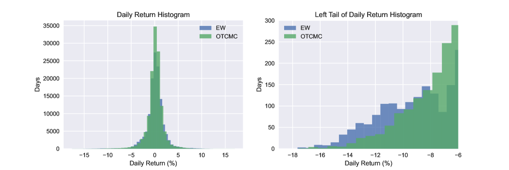
Figure 5. Histogram of the daily returns for EW and OTCMC. The daily returns are computed using the test period data from January 1, 2019 to December 31, 2020, thus each model contains $256\times 2$ years of data. The full histogram of daily return is presented in the left-hand side plot, while the right-hand side plot shows the left tails (return less than 6%) in detail.

Appendix E Implications for Contextual Two-stage Stochastic Linear programs

In this appendix, we explore how our distributionally robust conditional decision making framework can be exploited in a two-stage stochastic linear optimization problem. Let us redefine the loss function as $\ell(Y,\alpha,\beta)\triangleq r(h(Y,\alpha),\beta)-\eta\cdot h(Y,\alpha)$, where $h(Y,\alpha)$ captures the optimal profit generated by a linear recourse problem with right-hand side uncertainty:

$$h(y,\alpha)\triangleq\left\{\begin{array}[]{cl}\max&c^{\top}\upsilon\\ \operatorname{s.t.}&\upsilon\in\mathbb{R}^{m},~{}A\alpha+B\upsilon\leq Cy,\end{array}\right.$$

constrained by $K$ linear constraints prescribed by the matrices $A$, $B$ and $C$ of appropriate dimensions. This formulation can capture a number of interesting operational management problems including multi-item newsvendor problems [2], facility location problems [71], and scheduling problems [29].

In the case that $r(\cdot,\beta)$ is non-increasing for all $\beta$, such as for the CVaR formulation, one can obtain a conservative approximation for problem (1) by employing linear decision rules. Namely,

$$\mathds{E}_{\mathbb{P}}[\ell(Y,\alpha,\beta)]=\mathds{E}_{\mathbb{P}}[r(h(Y,\alpha),\beta)-\eta\cdot h(Y,\alpha)]\leq\mathds{E}_{\mathbb{P}}[r(c^{\top}(\upsilon+{\Upsilon}Y),\beta)-\eta\cdot c^{\top}(\upsilon+{\Upsilon}Y)]$$

as long as

$$A\alpha+B(\upsilon+{\Upsilon}y)\leq Cy\quad\forall y\in\mathcal{Y}$$ (42)

since in this case $h(y,\alpha)\geq c^{\top}(\upsilon+{\Upsilon}Y)$.

It is therefore not surprising that Propositions 3.4 and 4.6 have natural extensions to provide conservative approximation models in the form of second-order cone and semi-definite programs. As an example, Proposition 3.4 can be extended to the following.

Corollary E.1 (Mean-CVaR TSLP for single fiber set).

Suppose that $\ell$ is the mean-CVaR loss function of the form $\ell(y,\alpha,\beta)=-\eta h(y,\alpha)+\beta+\frac{1}{\tau}(-h(y,\alpha)-\beta)^{+}$, $\gamma=0$, $\varepsilon\in(0,1]$ and $\rho>\rho_{\min}(x_{0},0,\varepsilon)$. Suppose in addition that $\mathcal{X}=\mathbb{R}^{n}$, $\mathcal{Y}$ is polyhedral, $\mathbb{D}_{\mathcal{X}}(x,\widehat{x})=\|x-\widehat{x}\|^{2}$ and $\mathbb{D}_{\mathcal{Y}}(y,\widehat{y})=\|y-\widehat{y}\|_{2}^{2}$. The distributionally robust two-stage stochastic linear program with side information is conservatively approximated by the second-order cone program

$$\begin{array}[]{cll}\inf&\displaystyle\rho\lambda_{1}+\varepsilon\lambda_{2}-(1+\eta)c^{\top}\upsilon+\frac{1}{N}\sum_{i\in[N]}\theta_{i}\\ \operatorname{s.t.}&\alpha\in\mathcal{A},\;\beta\in\mathcal{B},\;\lambda_{1}\in\mathbb{R}_{+},\;\lambda_{2}\in\mathbb{R},\;\theta\in\mathbb{R}_{+}^{N},\;z\in\mathbb{R}_{+}^{N},\;\tilde{z}\in\mathbb{R}_{+}^{N},\;\upsilon\in\mathbb{R}^{m},\;{\Upsilon}\in\mathbb{R}^{m\times m}\\ &\left.\!\!\!\begin{array}[]{l}z_{i}=\theta_{i}+\lambda_{1}\|x_{0}-\widehat{x}_{i}\|^{2}+\lambda_{2}+\varepsilon^{-1}\eta\widehat{y}_{i}^{\top}{\Upsilon}^{\top}c-\varepsilon^{-1}\beta\\ \tilde{z}_{i}=\theta_{i}+\lambda_{1}\|x_{0}-\widehat{x}_{i}\|^{2}+\lambda_{2}+\varepsilon^{-1}(\eta+\frac{1}{\tau})\widehat{y}_{i}^{\top}{\Upsilon}^{\top}c-\varepsilon^{-1}(1-\frac{1}{\tau})\beta\\ \left\|\begin{bmatrix}\varepsilon^{-1}\eta{\Upsilon}^{\top}c\\ z_{i}-\lambda_{1}\end{bmatrix}\right\|_{2}\leq z_{i}+\lambda_{1},\quad\left\|\begin{bmatrix}\varepsilon^{-1}(\eta+\tau^{-1}){\Upsilon}^{\top}c\\ \tilde{z}_{i}-\lambda_{1}\end{bmatrix}\right\|_{2}\leq\tilde{z}_{i}+\lambda_{1}\end{array}\right\}\forall i\in[N]\\ &e_{k}^{\top}(A\alpha+B\upsilon)+\delta^{*}((\Upsilon^{\top}B^{\top}-C^{\top})e_{k}|\mathcal{Y})\leq 0\qquad\forall k\in[K],\end{array}$$ (43)

where $e_{k}$ is the $k$-th column of the identity matrix, and $\delta^{*}(z|\mathcal{Y})\triangleq\sup_{y\in\mathcal{Y}}z^{\top}y$ is a linear programming representable support function of $\mathcal{Y}$.

Proof of Corollary E.1.

We start with the following derivations

$$\min_{\beta} \sup\limits_{\mathbb{Q}\in\mathbb{B}_{\rho},\mathbb{Q}(X=x_{0})\geq\varepsilon}~{}\mathds{E}_{\mathbb{Q}}[\ell(Y,\alpha,\beta)|X=x_{0}]$$

$$\leq\min_{\beta}\sup\limits_{\mathbb{Q}\in\mathbb{B}_{\rho},\mathbb{Q}(X=x_{0})\geq\varepsilon}~{}\mathds{E}_{\mathbb{Q}}[r(c^{\top}(\upsilon+{\Upsilon}Y),\beta)-\eta\cdot c^{\top}(\upsilon+{\Upsilon}Y)|X=x_{0}]$$

$$=\min_{\beta}\sup\limits_{\mathbb{Q}\in\mathbb{B}_{\rho},\mathbb{Q}(X=x_{0})\geq\varepsilon}~{}\mathds{E}_{\mathbb{Q}}[-\eta c^{\top}(\upsilon+{\Upsilon}Y)+\beta+\frac{1}{\tau}(-c^{\top}(\upsilon+{\Upsilon}Y)-\beta)^{+}|X=x_{0}]$$

$$=-(1+\eta)c^{\top}\upsilon+\min_{\beta^{\prime}}\sup\limits_{\mathbb{Q}\in\mathbb{B}_{\rho},\mathbb{Q}(X=x_{0})\geq\varepsilon}~{}\mathds{E}_{\mathbb{Q}}[-\eta c^{\top}{\Upsilon}Y+\beta^{\prime}+\frac{1}{\tau}(-c^{\top}{\Upsilon}Y-\beta^{\prime})^{+}|X=x_{0}]$$

where we assume that the pair $(\upsilon,\Upsilon)$ satisfies the contraint (42), and where we perform the replacement $\beta^{\prime}\leftarrow\beta+c^{\top}\upsilon$. One obtains problem (43) after relaxing the support for $\mathbb{Q}$ to $\mathcal{X}\times\mathbb{R}^{m}$ in order to employ the reformulation proposed in Proposition 3.4, and finally reformulating each robust constraint, indexed by $k$, as:

$$e_{k}^{\top}(A\alpha+B\upsilon+(B{\Upsilon}-C)y)\leq 0\qquad\forall y\in\mathcal{Y}$$

using the definition of the support function. We refer the interested readers to [7] for examples of linear programming representations of support functions of polyhedral sets. ∎

References

- [1] C. D. Aliprantis and K. C. Border, Infinite Dimensional Analysis: A Hitchhiker’s Guide, Springer, 2006.
- [2] A. Ardestani-Jaafari and E. Delage, Linearized robust counterparts of two-stage robust optimization problems with applications in operations management, INFORMS Journal on Computing, 33 (2021), pp. 1138–1161.
- [3] P. Artzner, F. Delbaen, J.-M. Eber, and D. Heath, Coherent measures of risk, Mathematical Finance, 9 (1999), pp. 203–228.
- [4] S. Athey, J. Tibshirani, and S. Wager, Generalized random forests, Annals of Statistics, 47 (2019), pp. 1148–1178.
- [5] M. Baker and J. Wurgler, Investor sentiment and the cross-section of stock returns, The Journal of Finance, 61 (2006), pp. 1645–1680.
- [6] G.-Y. Ban and C. Rudin, The big data newsvendor: Practical insights from machine learning, Operations Research, 67 (2019), pp. 90–108.
- [7] A. Ben-Tal, D. D. Hertog, and J. Vial, Deriving robust counterparts of nonlinear uncertain inequalities, Mathematical Programming, 149 (2015), pp. 265–299.
- [8] S. Benati and R. Rizzi, A mixed integer linear programming formulation of the optimal mean/value-at-risk portfolio problem, European Journal of Operational Research, 176 (2007), pp. 423–434.
- [9] D. Bertsimas and N. Kallus, From predictive to prescriptive analytics, Management Science, 66 (2020), pp. 1025–1044.
- [10] D. Bertsimas and C. McCord, From predictions to prescriptions in multistage optimization problems, arXiv preprint arXiv:1904.11637, (2019).
- [11] D. Bertsimas, C. McCord, and B. Sturt, Dynamic optimization with side information, European Journal of Operational Research, (2022).
- [12] D. Bertsimas and B. V. Parys, Bootstrap robust prescriptive analytics, Mathematical Programming, (2021).
- [13] F. Black, Capital market equilibrium with restricted borrowing, The Journal of Business, 45 (1972), pp. 444–455.
- [14] J. Blanchet, L. Chen, and X. Y. Zhou, Distributionally robust mean-variance portfolio selection with Wasserstein distances, Management Science, forthcoming, (2018).
- [15] J. Blanchet, Y. Kang, and K. Murthy, Robust Wasserstein profile inference and applications to machine learning, Journal of Applied Probability, 56 (2019), pp. 830–857.
- [16] J. Blanchet and K. Murthy, Quantifying distributional model risk via optimal transport, Mathematics of Operations Research, 44 (2019), pp. 565–600.
- [17] J. Blanchet, K. Murthy, and V. A. Nguyen, Statistical analysis of Wasserstein distributionally robust estimators, INFORMS TutORials in Operations Research, (2021).
- [18] J. Blanchet, K. Murthy, and F. Zhang, Optimal transport based distributionally robust optimization: Structural properties and iterative schemes, arXiv preprint arXiv:1810.02403, (2018).
- [19] M. W. Brandt, P. Santa-Clara, and R. Valkanov, Parametric portfolio policies: Exploiting characteristics in the cross-section of equity returns, The Review of Financial Studies, 22 (2009), pp. 3411–3447.
- [20] M. Britten-Jones, The sampling error in estimates of mean-variance efficient portfolio weights, The Journal of Finance, 54 (1999), pp. 655–671.
- [21] Z. Chen, M. Sim, and P. Xiong, Robust stochastic optimization made easy with RSOME, Management Science, 66 (2020), pp. 3329–3339.
- [22] V. K. Chopra and W. T. Ziemba, The effect of errors in means, variances, and covariances on optimal portfolio choice, Journal of Portfolio Management, 19 (1993), p. 6.
- [23] G. B. Dantzig, Discrete-variable extremum problems, Operations Research, 5 (1957), pp. 266–277.
- [24] E. Delage and Y. Ye, Distributionally robust optimization under moment uncertainty with application to data-driven problems, Operations Research, 58 (2010), pp. 595–612.
- [25] V. DeMiguel, L. Garlappi, F. J. Nogales, and R. Uppal, A generalized approach to portfolio optimization: Improving performance by constraining portfolio norms, Management Science, 55 (2009), pp. 798–812.
- [26] V. DeMiguel, L. Garlappi, and R. Uppal, Optimal versus naive diversification: How inefficient is the 1/n portfolio strategy?, The Review of Financial Studies, 22 (2009), pp. 1915–1953.
- [27] V. DeMiguel, A. Martín-Utrera, F. J. Nogales, and R. Uppal, A transaction-cost perspective on the multitude of firm characteristics, The Review of Financial Studies, 33 (2020), pp. 2180––2222.
- [28] V. DeMiguel, Y. Plyakha, R. Uppal, and G. Vilkov, Improving portfolio selection using option-implied volatility and skewness, Journal of Financial and Quantitative Analysis, (2013), pp. 1813–1845.
- [29] B. T. Denton, A. J. Miller, H. J. Balasubramanian, and T. R. Huschka, Optimal allocation of surgery blocks to operating rooms under uncertainty, Operations Research, 58 (2010), pp. 802–816.
- [30] X. Dou and M. Anitescu, Distributionally robust optimization with correlated data from vector autoregressive processes, Operations Research Letters, 47 (2019), pp. 294–299.
- [31] J. Duchi and H. Namkoong, Learning models with uniform performance via distributionally robust optimization, arXiv preprint arXiv:1810.08750, (2018).
- [32] A. Esteban-Pérez and J. M. Morales, Distributionally robust stochastic programs with side information based on trimmings, Mathematical Programming, (2022).
- [33] F. J. Fabozzi, P. N. Kolm, D. A. Pachamanova, and S. M. Focardi, Robust portfolio optimization, The Journal of Portfolio Management, 33 (2007), pp. 40–48.
- [34] E. F. Fama and K. R. French, The cross-section of expected stock returns, The Journal of Finance, 47 (1992), pp. 427–465.
- [35] , Multifactor explanations of asset pricing anomalies, The Journal of Finance, 51 (1996), pp. 55–84.
- [36] J. Fan and I. Gijbels, Local Polynomial Modelling and Its Applications, no. 66 in Monographs on Statistics and Applied Probability Series, Chapman & Hall, 1996.
- [37] M. J. Flannery and A. A. Protopapadakis, Macroeconomic factors do influence aggregate stock returns, The Review of Financial Studies, 15 (2002), pp. 751–782.
- [38] H. Föllmer and A. Schied, Convex measures of risk and trading constraints, Finance and Stochastics, 6 (2002), pp. 429–447.
- [39] N. Fournier and A. Guillin, On the rate of convergence in Wasserstein distance of the empirical measure, Probability Theory and Related Fields, 162 (2015), pp. 707–738.
- [40] R. Gao and A. J. Kleywegt, Distributionally robust stochastic optimization with Wasserstein distance, arXiv preprint arXiv:1604.02199, (2016).
- [41] L. E. Ghaoui, M. Oks, and F. Oustry, Worst-case value-at-risk and robust portfolio optimization: A conic programming approach, Operations Research, 51 (2003), pp. 543–556.
- [42] J. Goh and M. Sim, Robust optimization made easy with ROME, Operations Research, 59 (2011), pp. 973–985.
- [43] M. Grinblatt, S. Titman, and R. Wermers, Momentum investment strategies, portfolio performance, and herding: A study of mutual fund behavior, The American Economic Review, (1995), pp. 1088–1105.
- [44] R. Ji and M. A. Lejeune, Data-driven optimization of reward-risk ratio measures, INFORMS Journal on Computing, (2021).
- [45] N. Kallus and X. Mao, Stochastic optimization forests, arXiv preprint arXiv:2008.07473, (2020).
- [46] R. Kannan, G. Bayraksan, and J. R. Luedtke, Data-driven sample average approximation with covariate information, Available from Optimization Online, (2020).
- [47] , Heteroscedasticity-aware residuals-based contextual stochastic optimization, arXiv preprint arXiv:2101.03139, (2020).
- [48] , Residuals-based distributionally robust optimization with covariate information, arXiv preprint arXiv:2012.01088, (2020).
- [49] H. Konno and H. Yamazaki, Mean-absolute deviation portfolio optimization model and its applications to Tokyo stock market, Management Science, 37 (1991), pp. 519–531.
- [50] B. Korte and J. Vygen, Combinatorial Optimization: Theory and Algorithms, Springer, 2007.
- [51] S. Kozak, S. Nagel, and S. Santosh, Shrinking the cross-section, Journal of Financial Economics, 135 (2020), pp. 271–292.
- [52] D. Kuhn, P. Mohajerin Esfahani, V. A. Nguyen, and S. Shafieezadeh-Abadeh, Wasserstein distributionally robust optimization: Theory and applications in machine learning, in Operations Research & Management Science in the Age of Analytics, 2019, pp. 130–166.
- [53] M. S. Lobo and S. Boyd, The worst-case risk of a portfolio, Unpublished Manuscript, (2000).
- [54] M. S. Lobo, L. Vandenberghe, S. Boyd, and H. Lebret, Applications of second-order cone programming, Linear Algebra and Its Applications, 284 (1998), pp. 193–228.
- [55] H.-J. Lüthi and J. Doege, Convex risk measures for portfolio optimization and concepts of flexibility, Mathematical Programming, 104 (2005), pp. 541–559.
- [56] H. Markowitz, Portfolio selection, The Journal of Finance, 7 (1952), pp. 77–91.
- [57] P. Mohajerin Esfahani and D. Kuhn, Data-driven distributionally robust optimization using the Wasserstein metric: Performance guarantees and tractable reformulations, Mathematical Programming, 171 (2018), pp. 115–166.
- [58] MOSEK ApS, MOSEK Optimizer API for Python 9.2.10, 2019.
- [59] K. Natarajan, M. Sim, and J. Uichanco, Tractable robust expected utility and risk models for portfolio optimization, Mathematical Finance, 20 (2010), pp. 695–731.
- [60] C. J. Neely, D. E. Rapach, J. Tu, and G. Zhou, Forecasting the equity risk premium: The role of technical indicators, Management Science, 60 (2014), pp. 1772–1791.
- [61] V. A. Nguyen, F. Zhang, J. Blanchet, E. Delage, and Y. Ye, Distributionally robust local non-parametric conditional estimation, in Advances in Neural Information Processing Systems 33, 2020.
- [62] L. Pástor and R. F. Stambaugh, Liquidity risk and expected stock returns, Journal of Political Economy, 111 (2003), pp. 642–685.
- [63] G. Pflug, A. Pichler, and D. Wozabal, The investment strategy is optimal under high model ambiguity, Journal of Banking & Finance, 36 (2012), pp. 410–417.
- [64] G. Pflug and D. Wozabal, Ambiguity in portfolio selection, Quantitative Finance, 7 (2007), pp. 435–442.
- [65] I. Pólik and T. Terlaky, A survey of the -lemma, SIAM Review, 49 (2007), pp. 371–418.
- [66] M. Qi, Y. Cao, and Z.-J. M. Shen, Distributionally robust conditional quantile prediction with fixed design, Management Science, 68 (2022), pp. 1639–1658.
- [67] H. Rahimian and S. Mehrotra, Distributionally robust optimization: A review, arXiv preprint arXiv:1908.05659, (2020).
- [68] H. Rahimian and B. Pagnoncelli, Contextual chance-constrained programming, Available on Optimization Online, (2020).
- [69] D. E. Rapach, M. C. Ringgenberg, and G. Zhou, Short interest and aggregate stock returns, Journal of Financial Economics, 121 (2016), pp. 46–65.
- [70] R. T. Rockafellar and S. Uryasev, Optimization of Conditional Value-at-Risk, Journal of Risk, 2 (2000), pp. 21–41.
- [71] A. Saif and E. Delage, Data-driven distributionally robust capacitated facility location problem, European Journal of Operational Research, 291 (2021), pp. 995–1007.
- [72] S. Schaible, Parameter-free convex equivalent and dual programs of fractional programming problems, Zeitschrift für Operations Research, 18 (1974), pp. 187–196.
- [73] A. Shapiro, On duality theory of conic linear problems, in Semi-Infinite Programming, Kluwer Academic Publishers, 2001, pp. 135–165.
- [74] W. F. Sharpe, Capital asset prices: A theory of market equilibrium under conditions of risk, The Journal of Finance, 19 (1964), pp. 425–442.
- [75] N. Si, K. Murthy, J. Blanchet, and V. A. Nguyen, Testing group fairness via optimal transport projections, in Proceedings of the 38th International Conference on Machine Learning, 2021.
- [76] M. Sion, On general minimax theorems, Pacific Journal of Mathematics, 8 (1958), pp. 171–176.
- [77] J. E. Smith, Generalized Chebychev inequalities: Theory and applications in decision analysis, Operations Research, 43 (1995), pp. 807–825.
- [78] P. R. Srivastava, Y. Wang, G. A. Hanasusanto, and C. P. Ho, On data-driven prescriptive analytics with side information: A regularized Nadaraya-Watson approach, arXiv preprint arXiv:2110.04855, (2021).
- [79] R. Uppal and T. Wang, Model misspecification and underdiversification, The Journal of Finance, 58 (2003), pp. 2465–2486.
- [80] C. Villani, Optimal Transport: Old and New, Springer, 2008.
- [81] F. Wilcoxon, Individual comparisons by ranking methods, in Breakthroughs in Statistics, Springer, 1992, pp. 196–202.
- [82] C. Zhao and Y. Guan, Data-driven risk-averse stochastic optimization with Wasserstein metric, Operations Research Letters, 46 (2018), pp. 262 – 267.
- [83] Y. Zhao, Y. Liu, J. Zhang, and X. Yang, Distributionally robust reward-risk ratio programming with Wasserstein metric, Available on Optimization Online, (2017).
- [84] S. Zhu and M. Fukushima, Worst-case conditional value-at-risk with application to robust portfolio management, Operations Research, 57 (2009), pp. 1155–1168.
- [85] S. Zymler, D. Kuhn, and B. Rustem, Distributionally robust joint chance constraints with second-order moment information, Mathematical Programming, 137 (2013), pp. 167–198.