Variational models for signal processing
with Graph Neural Networks

Abstract

This paper is devoted to signal processing on point-clouds by means of neural networks. Nowadays, state-of-the-art in image processing and computer vision is mostly based on training deep convolutional neural networks on large datasets. While it is also the case for the processing of point-clouds with Graph Neural Networks (GNN), the focus has been largely given to high-level tasks such as classification and segmentation using supervised learning on labeled datasets such as ShapeNet. Yet, such datasets are scarce and time-consuming to build depending on the target application. In this work, we investigate the use of variational models for such GNN to process signals on graphs for unsupervised learning.

Our contributions are two-fold. We first show that some existing variational - based algorithms for signals on graphs can be formulated as Message Passing Networks (MPN), a particular instance of GNN, making them computationally efficient in practice when compared to standard gradient-based machine learning algorithms. Secondly, we investigate the unsupervised learning of feed-forward GNN, either by direct optimization of an inverse problem or by model distillation from variational-based MPN.

1 Introduction

Variational methods have been a popular framework for signal processing since the last few decades. Although, with the advent of deep Convolutional Neural Networks (CNN), most computer vision tasks and image processing problems are nowadays addressed using state-of-the-art machine learning techniques. Recently, there has been a growing interest in hybrid approaches combining machine learning techniques with variational modeling have seen a (see e.g. [19, 15, 1, 4, 11]).

1.0.1 Motivations.

In this paper, we focus on such hybrid approaches for processing of point-clouds and signals on graphs. Graph representation provides a unified framework to work with regular and irregular data, such as images, text, sound, manifold, social network and arbitrary high dimensional data. Recently, many machine learning approaches have also been proposed to deal with high-level computer vision tasks, such as classification and segmentation [21, 22, 28], point-cloud generation [31], surface reconstruction [29], point cloud registration [27] and up-sampling [16] to name a few. These approaches are built upon Graph Neural Networks (GNN) which are inspired by powerful techniques employed in CNN, such as Multi-Linear Perceptron (MLP), pooling, convolution, etc. The main caveat is that transposing CNN architectures for graph-like inputs is not a simple task. Compared to images which are defined on a standard, regular grid that can be easily sampled, data with graph structures can have a large structural variability, which makes the design of a universal architecture difficult. This is likely the main reason why GNN are still hardly being used for signal processing on graph for which variational methods are still very popular. In this work, we investigate the use of data-driven machine learning techniques combined with variational models to solve inverse problems on point clouds.

1.1 Related work

1.1.1 Graph Neural Networks

GNN are types of Neural Networks which directly operate on the graph structure. GNN are emerging as a strong tool to do representation learning on various types of data which, similarly to CNN, can hierarchically learn complex features.

PointNet [21] was one of the first few successful attempts to build GNN. Rather than preprocessing the input point-cloud by casting it into a generic structure, Qi et al. proposed to tackle the problem of structure irregularity by only considering permutation invariant operators that are applied to each vertex independently. Further works such as [22] have built upon this framework to replicate other successful NN techniques, such as pooling and interpolation in auto-encoder, which enables to process neighborhood of points.

Most successful attempts to build Graph Convolutional Networks (GCN) were based upon graph spectral theory (see for instance [2, 5, 14]). In particular, Kipf and Welling [14] proposed a simple, linear propagation rule which can be seen as a first-order approximation of local spectral filters on graphs. More recently, Wang et al. introduced an edge convolution technique [28] which maintains the permutation invariance property. Interestingly, [30] showed that GCN may act as low pass filters on internal features.

1.1.2 Message Passing Networks

At the core of the most the aforementioned GNNs, is Message Passing (MP). The term was first coined in [10], in which authors proposed a common framework that reformulated many existing GNNs, such as [2, 21, 14]. In the simplest terms, MP is a generalized convolution operator on irregular domains which typically expresses some neighborhood aggregation mechanism consisting of a message function, a permutation invariant function (e.g. $\max$) and an update function.

1.1.3 Inverse problems on Graphs.

PDEs and variational methods are two major frameworks to address inverse problems on a regular grid structure like images. These methods have also been extended to weighted graphs in non-local form by defining $p$-Laplace operators [7]. Typical but not limited applications of these operators are filtering, classification, segmentation, or inpainting [20]. Specifically, we are interested in this work in non-local Total-Variation on a graph, which has been thoroughly studied, e.g. for non-local signal processing [6, 9, 25], multi-scale decomposition of signals [12], point-cloud segmentation [18] and sparsification [26], using various optimization schemes (such as finite difference schemes [6], primal-dual [3], forward-backward [23], or cut pursuit [24]).

1.1.4 Contributions and Outline

The paper is organised as follows. Section 2 focus on variational methods to solve inverse problems for graph signal processing. After a short overview of graph representation and non-local regularization, we demonstrate that two popular optimization algorithms can be interpreted as a specific instance of Message Passing Networks (MPNs). This allows using efficient GPU-based machine learning libraries to solve the inverse problem on graphs. Experiments on point cloud compression and color processing show that such MPN optimization is more efficient than standard machine learning optimization techniques. Section 3 is devoted to the use of a trainable GNN to perform signal processing on graphs in a feed-forward fashion. We investigate two techniques for unsupervised training, i.e. in absence of ground-truth data, using variational models as prior knowledge to drive the optimization. We show that either model distillation from a variational MPN or optimizing the inverse problem directly with GNN gives satisfactory approximate solutions and allows for faster processing.

2 Solving Inverse Problem with MPN optimization

2.1 Notations and definitions

A graph $\mathcal{G}=(\mathcal{V},\mathcal{E},\omega)$ is composed of an ensemble of nodes (vertices) $\mathcal{V}$, an ensemble of edges $\mathcal{E}=\mathcal{V}\times\mathcal{V}$ and weights $\omega:\mathcal{E}\mapsto\mathbb{R}_{+}$, where $\mathbb{R}_{+}$ indicates the set of non-negative values $[0,\infty)$. Let $f_{i}\in\mathbb{R}^{d}$ represents the feature vector (signal) on the node $i$ of $\mathcal{G}$, $w_{i,j}$ the scalar weight on the edge from the node $i$ to $j$, and $j\in\mathcal{N}(i)$ indicates a node $j$ in the neighborhood of node $i$, such that $\omega_{i,j}\neq 0$. For sake of simplicity, we only consider non-directed graph, i.e. defined with symmetric weights $\omega_{i,j}=\omega_{j,i}$.

We refer to the weighted difference operator as $\nabla_{\omega}$: $(\nabla_{\omega}f)_{i,j}=\sqrt{\omega_{i,j}}\left(f_{j}-f_{i}\right)\in\mathbb{R}^{d}$ , ${\forall\ (i,j)\in\mathcal{E}}$. Assuming symmetry of $\omega$, the adjoint of this linear operator is $(\nabla^{\ast}_{\omega}g)_{i}=\sum_{j\in\cal V}\sqrt{\omega_{i,j}}\left(g_{j,i}-g_{i,j}\right)\in\mathbb{R}^{d},\forall\ i\in\mathcal{V}.$ We denote as $\|.\|_{p}$ the $\ell_{p}$ norm and $\|.\|_{1,p}$ the composed norm for parameter $p\in\mathbb{R}_{+}\cup\{\infty\}$:

$$\forall\ g\in\mathbb{R}^{|\mathcal{V}|\times|\mathcal{V}|\times d},\;\|g\|_{1,p}=\sum_{i\in\mathcal{V}}\|g_{i,.}\|_{p}=\sum_{i\in\mathcal{V}}\Big{(}\sum_{j\in\mathcal{V},1\leq k\leq d}|g_{i,j,k}|^{p}\Big{)}^{1/p}.$$

2.2 Non-Local Regularization on Graph

In this work, we focus on inverse problems for signal processing on graph using the non-local regularization framework [6]. The optimization problem is formulated generically using $\ell_{2}$ fidelity term and a non-local regularization defined from the $\ell^{p}$ norm, parametrized by weights $\omega$ and power coefficient $q\in\mathbb{R}_{+}$, and penalized by $\lambda\in\mathbb{R}_{+}$

$$\inf_{f}\left\{{J}(f):=\tfrac{1}{2}\|f-f_{0}\|^{2}+\tfrac{\lambda}{q}\text{R}_{p}^{q}(f)\right\}\text{ where }\text{R}_{p}^{q}(f)={\|\nabla_{\omega}f\|}_{1,p}^{q}.$$ (1)

Here $f_{0}$ is the given signal which requires processing. In experiments, we will mainly focus on two cases: when $p=q=2$, the smooth regularization term relates to the Tikhonov regularization and boils down to Laplacian diffusion on a graph [6]. For $q=1$, the regularization term is the Non-Local Total Variation (NL-TV), referred to as isotropic when $p=2$ and anisotropic when $p=1$. Other choice of norm might be useful: using $p\leq 1$, as studied for instance for $p=0$ in [26], results in sparsification of signals; using $p=\infty$ [25] is also useful when considering unbiased symmetric schemes.

As the functional $J$ is not smooth, an $\varepsilon$-approximation $J_{\varepsilon}$ is often considered to circumvent numerical problems (see e.g. [6]); this is for instance achieved by substituting the term $R_{p}^{q}$ with (respectively for the case $p=2$ and $p=1$)

$$\text{R}^{q}_{2,\varepsilon}(f)=\sum_{i\in\mathcal{V}}\left(\|\nabla_{\omega}f_{i,.}\|_{p}^{2}+\varepsilon^{2}\right)^{\frac{q}{2}}\text{ and }\text{R}^{q}_{1,\varepsilon}(f)=\sum_{i,j\in\mathcal{V}}\omega_{i,j}^{\frac{q}{2}}\left(|f_{i}-f_{j}|+\varepsilon\right)^{q}.$$ (2)

2.3 Variational Optimization

We consider now two popular algorithms to solve inverse problem (1), described in Alg. 1 and 2 with update rules on $f^{(t)}$, where $(t)$ is the iteration number.

  Initialization: $f^{(0)}=f_{0}$, set $\varepsilon>0$   compute $\gamma^{(t)}_{i,j}$ using Eq.(3)   $\bar{f}^{(t+1)}_{i}=(f_{0})_{i}+\lambda\sum_{j\in\mathcal{N}_{i}}\gamma^{(t)}_{i,j}f^{(t)}_{j}$   $g^{(t+1)}_{i}=1+\lambda\sum_{j\in\mathcal{N}_{i}}\gamma^{(t)}_{i,j}$   $f^{(t+1)}_{i}={\bar{f}^{(t+1)}_{i}}/{g^{(t+1)}_{i}}$

Algorithm 1 Gauss-Jacobi [6]

     Parameters: $\tau,\beta>0$ and $\theta\in[0,1]$   Initialization: $f^{(0)}=\bar{f}^{(0)}=f_{0}$   $g^{(t+1)}=\operatorname{Prox}_{\beta A^{\ast}}(g^{(t)}+\beta K\bar{f}^{(t)})$   $f^{(t+1)}=\operatorname{Prox}_{\tau B}(f^{(t)}-\tau K^{\ast}g^{(t+1)})$   $\bar{f}^{(t+1)}=f^{(t+1)}+\theta(f^{(t+1)}-f^{(t)})$ Algorithm 2 Primal-Dual [3]

For any $p,q>0$, one can turn to the Gauss-Jacobi (GS) iterated filter [6] described in Alg. 1. It relies on $\varepsilon$ approximation to derive the objective function, giving for instance the following update rule when using Eq. (2)

$$\gamma^{(t)}_{i,j}=\begin{cases}w_{i,j}\left((\|(\nabla_{w}f)_{i,.}\|^{2}+\varepsilon^{2})^{\frac{q-2}{2}}+(\|(\nabla_{w}f)_{j,.}\|^{2}+\varepsilon^{2})^{\frac{q-2}{2}}\right)&\text{if }p=2\\ 2{w_{i,j}}^{\frac{q}{2}}\left(|f_{i}-f_{j}|+\varepsilon\right)^{q-2}&\text{if }p=1\end{cases}.$$ (3)

When considering the specific case of NL-TV ($q=1$), one can turn to the primal-dual algorithm [3] described in Alg. 2, as done in [18, 12]. To do so, we recast the problem (1) as $\min_{f}\max_{g}\langle Kf,\,g\rangle-A^{\ast}(g)+B(f)$ where $K\equiv\nabla_{\omega}$, $A\equiv{\|.\|}_{1,p}$, $B\equiv\tfrac{1}{2\lambda}{\|.-f_{0}\|}_{2}^{2}$. Parameters must be chosen such that $\tau\beta|\!|K|\!|^{2}<1$ to ensure convergence. For numerical experiments, we have used $\theta=1$ and $\tau=\beta=(4\max_{i\in\mathcal{V}}\sum_{j\in\mathcal{V}}\omega_{i,j})^{-1}$. Note that other methods might be used, such as pre-conditioning [23], and cut pursuit [24]. Proximal operators corresponds to

$$\operatorname{Prox}_{\tau B}(f)=\tfrac{\lambda f+\tau f_{0}}{\lambda+\tau}\;,\quad\text{ and }\operatorname{Prox}_{\beta A^{*}}(g)=\operatorname{Proj}_{\mathcal{B}_{\infty,p^{\prime}}}(g)$$ (4)

where the dual norm parameter $p^{\prime}>0$ verifies $1/p^{\prime}+1/p=1$. The projection on the unit ball $\mathcal{B}_{\infty,p^{\prime}}$ for $p=2$ and $p=1$ is given respectively by, $\forall\ g\in\mathbb{R}^{|\mathcal{V}|\times|\mathcal{V}|\times d}$

$$\operatorname{Proj}_{\mathcal{B}_{\infty,2}}(g)_{i,j,k}=\frac{g_{i,j,k}}{\max\{1,{\|g_{i,.}\|}_{2}\}}\;,\operatorname{Proj}_{\mathcal{B}_{\infty,\infty}}(g)_{i,j,k}=\frac{g_{i,j,k}}{\max\{1,|g_{i,j,k}|\}}.$$ (5)

2.4 Message Passing Network Optimization

Message Passing Networks [10] can be formulated as follows

$${f}_{i}^{(n+1)}=\psi^{(n)}\left({f}_{i}^{(n)},\square{}_{j\in\mathcal{N}(i)}\ \phi^{(n)}\left({f}_{i}^{(n)},{f}_{j}^{(n)},\omega_{i,j}\right)\right)\quad\forall\ i\in\mathcal{V},\;$$ (6)

where $(n)$ indicates the depth in the network. As already shown in [10], many existing GNN can be recast in this generic framework. Typically, $\square{}$ is the summation operator but can be any differentiable permutation invariant functions (such as $\max$, mean); $\psi^{(n)}$ (update rule) and $\phi^{(n)}$ (message rule) are the differentiable operators, such as MLPs (i.e. affine functions combined with simple non-linear functions such as RELU). Note that they are independent of the input vertex index to preserve permutation invariance.

We now show that Alg. 1 and 2 can be also formulated within this framework.

G-J algorithm.

This is quite straightforward for the anisotropic case ($p=1$) using two MPNs to compute the update of $f$ in Alg. 1. A first MPN is used for the numerator $\bar{f}$, identifying $\psi^{(n)}(f_{i}^{(n)},F_{i}^{(n)})=(f_{0})_{i}+\lambda F_{i}^{(n)}$, $\square{}=\sum$ and $\phi^{(n)}(f_{i}^{(n)},f_{j}^{(n)},\omega_{ij})=\gamma_{i,j}^{(n)}f_{j}^{(n)}$ where $\gamma_{i,j}^{(n)}$, as defined in Eq. (3), is a function of the triplet $(f_{i}^{(n)},f_{j}^{(n)},\omega_{i,j})$. A second MPN is used to compute the denominator $g$ using $\psi^{(n)}(f_{i}^{(n)},F_{i}^{(n)})=1+\lambda F_{i}^{(n)}$ and $\phi^{(n)}(f_{i}^{(n)},f_{j}^{(n)},\omega_{ij})=\gamma_{i,j}^{(n)}$. For the isotropic case $p=2$, an additional MPN is ultimately required to compute the norm of the gradient $(Kf^{(n)})_{i}$ at each vertex $i$, as detailed in the next paragraph.

P-D algorithm.

Two nested MPNs are now required to compute the update of the primal variable $f$ and the dual variable $g$ in Alg. 2. For $f$, the MPN reads as the affine operator $\psi^{(n)}(f_{i}^{(n)},{F}_{i}^{(n)})=\tfrac{\tau}{\tau+\lambda}(f_{0})_{i}+\tfrac{\tau}{\tau+\lambda}(f_{i}^{(n)}-\tau{F}_{i}^{(n)})$. Similarly, for the update of $g$ one computes the projection: $\psi^{(n)}(g_{i}^{(n)},{G}_{i}^{(n)})=\operatorname{Proj}_{\mathcal{B}_{\infty,p^{\prime}}}(g_{i}^{(n)}+\beta{G}_{i}^{(n)}).$ The gradient operator $K$ and its adjoint $K^{*}$ (see definition in §. 2.1) can be applied using the processing functions $\phi$ and $\phi_{j}$, respectively

$${G}_{i}^{(n)}=(K\bar{f}^{(n)})_{i}=\phi^{(n)}(\bar{f}_{i}^{(n)},\bar{f}_{j}^{(n)},\omega_{i,j})=\omega_{i,j}(\bar{f}_{j}^{(n)}-\bar{f}_{i}^{(n)})$$

$${F}_{i}^{(n)}=(K^{*}g^{(n+1)}))_{i}=\square{}\phi_{j}^{(n)}(g_{i}^{(n+1)},g_{j}^{(n+1)},\omega_{i,j})=\sum_{j\in{N}_{i}}\omega_{i,j}(g_{j,i}^{(n+1)}-g_{i,j}^{(n+1)})$$

Observe that $\phi_{j}$ is a slightly modified message passing function using index $j$ to incorporate the edge features from not only source $i$ to target $j$ (i.e. $g_{i,j}$ and $\omega_{i,j}$) but also from target $j$ to source $i$ ($g_{j,i}$ and $\omega_{j,i}$).

These MPN formulations of Alg. 1 and Alg. 2 allows to use machine learning libraries to solve the inverse problem Eq. 1 and to take full advantage of fast GPU optimization. In the following experiments, we illustrate the advantage of such MPN optimization in comparison with standard gradient-based machine learning optimization techniques relying on auto-differentiation.

2.5 Experiments on point-clouds and comparison with auto-diff

Experimental setting.

Edges on point-clouds are defined with weights $\omega_{i,j}\in\{0,1\}$ using the indicator function of a k-nearest neighbor search ($k=4$) on points coordinates using $\ell_{2}$ norm, then imposing symmetry by setting $\omega_{i,j}\leftarrow\omega_{i,j}\vee\omega_{j,i}$. Two types of features $f$ are tested for $q=1$, as illustrated in Fig. 1: 3D point coordinates $x$ for point-cloud simplification (Fig. 2), and colors $c\in[0,1]^{|\mathcal{V}|\times 3}$ for denoising (Fig. 3). We also consider the non-convex case where $q=0.1$ for point cloud sparsification in Fig. 2.

Auto-differentiation.

As a baseline, we compare these MPN-based algorithms with algorithmic auto-differentiation. In this setting, the update of features at iteration $(t)$ is defined by gradient descent on the loss function $J(f^{(t)})$ defined in Eq. (1), e.g. $f^{(t+1)}=f^{(t)}-\rho^{(t)}D^{(t)}$. Since the NL-TV regularization term is not smooth, we use the $\varepsilon$ approximation of Eq. (2) to compute the gradient $D^{(t)}$. We consider here various standard gradient descent techniques used for NN training: Gradient Descent (gd), adam [13] and lbfgs [17].

Implementation details.

All algorithms are implemented using the Pytorch Geometric library [8] and tested with a Nvidia GPU GTX1080Ti with 11 GB of memory. Note that reported computation time is only indicative, as implementation greatly influence the efficiency of memory and GPU cores allocation. Different learning rates are used for each method in the experiments. The learning rate of adam algorithm is always set to $lr=0.001$. gd is also used with $lr=0.001$ for point-cloud simplification but with $lr=0.1$ for color processing. lbfgs is set with $lr=0.01$ for $q=1$, and with $lr=0.1$ for $q=0.1$.

Features $f_{0}$	$q=1$, $p=2$	$q=1$, $p=1$	$q=0.1$, $p=2$

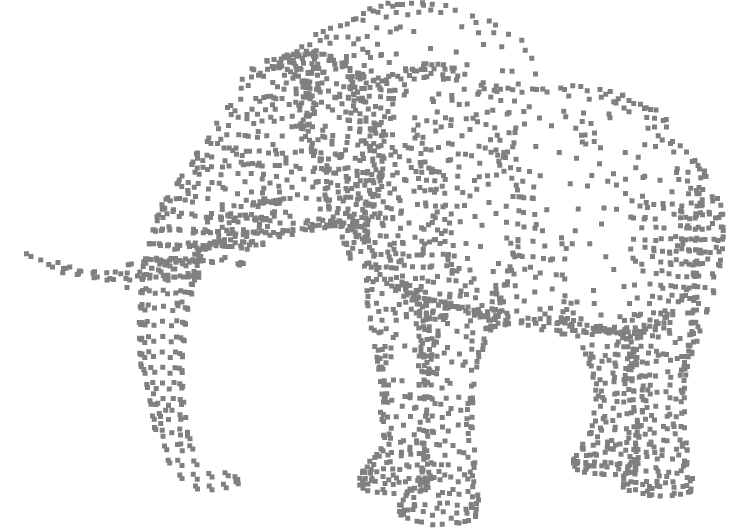
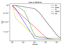
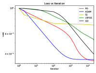
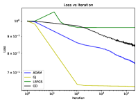
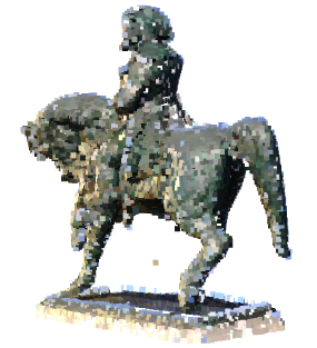
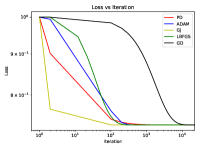
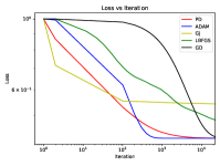
Figure 1: (left) Raw data $f_{0}$ used for experiments in Fig. 2 and Fig. 3. (right) Comparison of the evolution of the objective function $J(f^{(t)})$ depending on iteration $(t)$, in logarithmic scale, for various setting of $(p,q)$ and for different algorithms.

	mpn-pd	mpn-gj	gd	adam	lbfgs
$q=1$ $p=2$
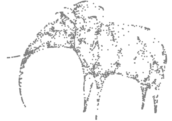
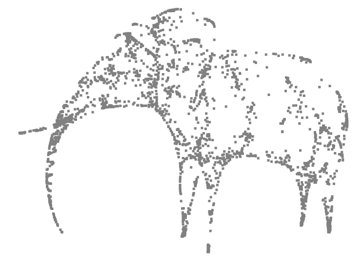
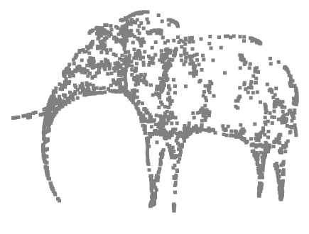
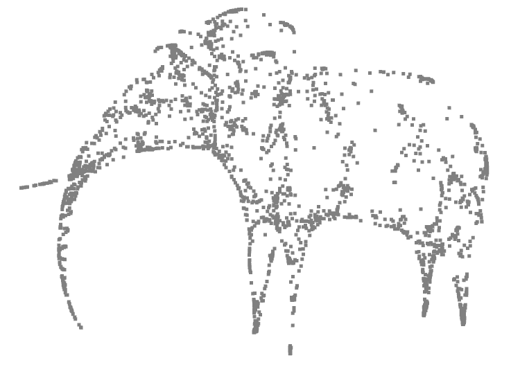
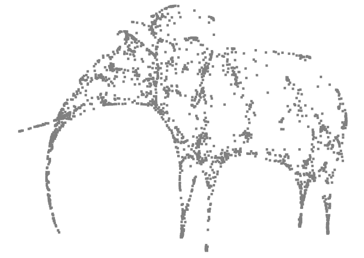
$q=1$ $p=1$
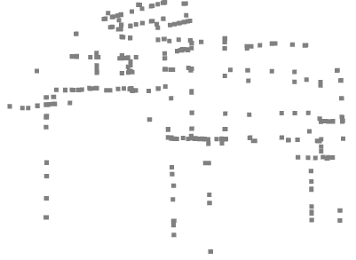
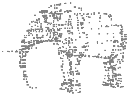
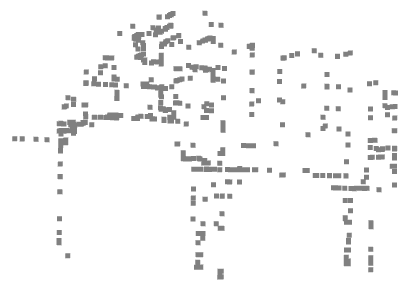
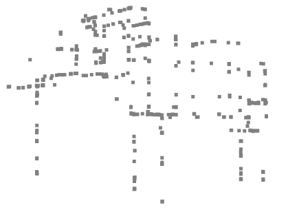
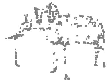
$q=0.1$ $p=2$

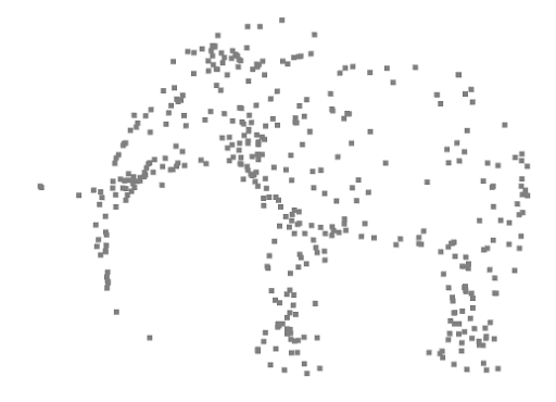
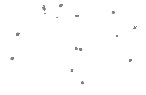
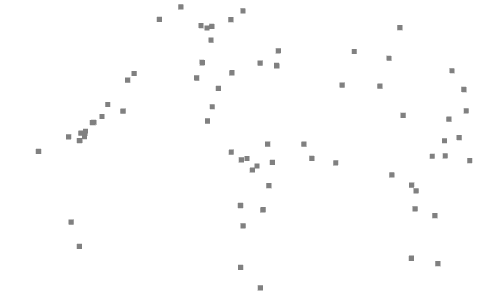
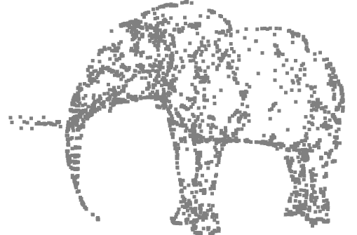
Figure 2: Comparison of numerical results of MPN implementations of algorithms 1 (mpn-gj) and 2 (mpn-pd), with gd, adam and lbfgs after $20k$ iterations. Point-cloud simplification is defined by problem (1) with $\lambda=0.2$ and various settings of $p$ and $q$. For all methods except mpn-pd, the approximated formulation (2) with $\epsilon=10^{-8}$ is used.

	mpn-pd	mpn-gj	gd	adam	lbfgs
$p=2$
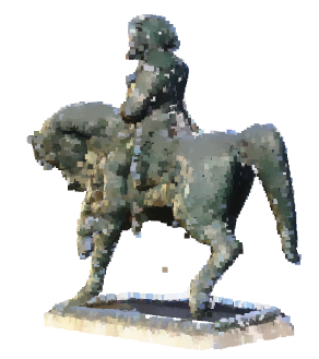
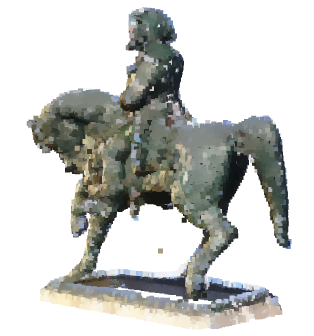
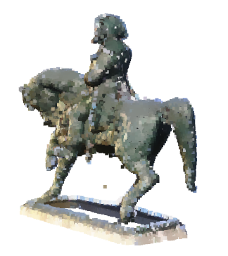
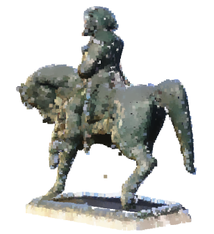
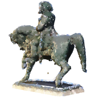
$p=1$

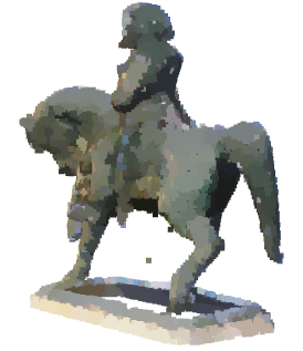
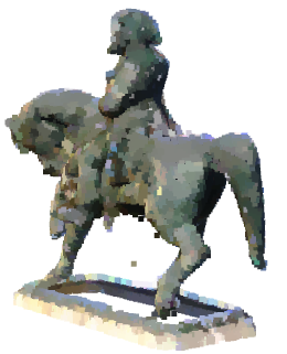
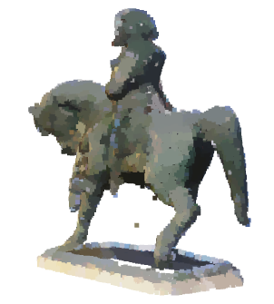
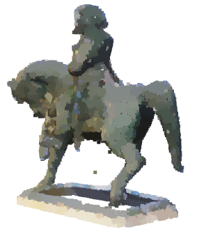
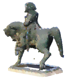
Figure 3: Same setting as in Fig. 2 except $\lambda=0.05$, for color processing.

Results.

Observe that the noise on the raw color point cloud in Fig. 1 results from the registration of multiple scans with different lighting conditions, for which we do not have any ground-truth. In such a case, variational models like in (1) are useful to remove color artifacts without more specific prior knowledge.

Figures 2 and 3 show the visual results of the aforementioned algorithms after 20k iterations. The objective function $J(f^{(t)})$ is plotted for each one in Fig. 1. Since the computation time per iteration is roughly same for all methods (about 0.5 ms for mpn-pd and 1 ms for others on ‘elephant’ and ‘Napoléon’ pointclouds with $|\mathcal{V}|=3k$ and $11k$ respectively), curves are here simply displayed versus the number of iterations. As one can observe from these experiments, MPN based algorithms perform better than gradient based algorithm when it comes to precision. Indeed, for $q=1$, Alg. 2 is the only algorithm that can be used without approximation (i.e. $\varepsilon=0$, which is numerically intractable for other methods) and that gives ultimately an optimal solution. As for $q=0.1$, Alg. 1 reaches an (approximated) solution much faster than gradient based methods. Among these, it is interesting to notice that adam is quite consistent and performs quite well. For this reason, we will consider this method for the next part devoted to unsupervised training of GNN.

We have shown that the two algorithms can be implemented efficiently as MPN, a special instance of GNN. In the next section, we demonstrate the interest of training such MPNs to design feed-forward GNNs allowing fast processing.

3 Variational training of GNN

One of the most attractive aspect of machine learning is the ability to learn the model itself from the data. As already mentioned in the introduction, most approaches rely on supervised training techniques which require datasets with ground-truth, potentially obtained by means of data augmentation (i.e. artificially degrading the data), which might be a simple task for some applications such as Gaussian denoising on images. However, it is challenging and time consuming to achieve this for signal processing tasks on point-clouds. Besides, most of the available datasets are only devoted to high-level tasks like segmentation and classification on shapes.

Inspired from the previous results, we investigate the unsupervised training of a GNN to reproduce the behavior of variational models on point-clouds while reducing the computation time. To achieve such a goal, two different settings are considered in this section: Unsupervised training using the variational energy as a loss function (§ 3.1), and model distillation using exemplars from the variational model defined as an MPN (§ 3.2).

3.1 Unsupervised training

We denote by $G_{\theta}:\mathbb{R}^{|\mathcal{V}|\times d}\times\mathbb{R}_{+}^{\mathcal{E}}\to\mathbb{R}^{|\mathcal{V}|\times d}$ a trainable GNN parametrized by $\theta$, processing a graph defined by the vertex features $f$ and the edge weights $\omega$. The idea here is simply to train a GNN in such a way that it minimizes in expectation the objective function (1) of the variational model for graphs from a dataset

$$\inf_{\theta}\mathbb{E}_{X\sim P_{\text{data}}}J\left(G_{\theta}(X,\omega(X))\right).$$ (7)

where $X$ is a random point-cloud (and its associated weights $\omega(X)$) from the training dataset with probability distribution $P_{\text{data}}$. Once again, in practice, we need to consider the $\varepsilon$-approximation $J_{\varepsilon}$ (2) to overcome numerical issues.

3.2 Model distillation with MPN

As seen above, the main caveat in variational training is that it requires smoothing if the objective function is not differentiable. to avoid this limitation, we consider another setting which consists of model distillation, where the goal is to train a gnn to reproduce an exact model defined by a mpn.

Let $F:\mathbb{R}^{|\mathcal{V}|\times d}\times\mathbb{R}_{+}^{\mathcal{E}}\mapsto\mathbb{R}^{|\mathcal{V}|\times d}$ denotes a MPN designed to solve a variational model, such as mpn-pd in the previous section for the NL-TV model. Note that in practice, we have to restrict this network to $n$ updates. Using for instance $\ell_{2}$ norm, the distillation training boils down to the following optimization problem

$$\inf_{\theta}\mathbb{E}_{X\sim P_{\text{data}}}\lVert G_{\theta}(X,\omega(X))-F(X,\omega(X))\rVert^{2}$$ (8)

Other choices of distance could be as well considered, such as $\ell_{1}$ norm or optimal transport cost for instance [29].

3.3 Experiments

Dataset setting.

We use the same experimental setting as in the previous section, except that $k$ nearest-neighbor parameters $\omega_{i,j}\in\{0,1\}$ are now weighted using features proximity: $\omega_{i,j}\leftarrow\omega_{i,j}e^{-\kappa\|(f_{0})_{i}-(f_{0})_{j}\|^{2}}$ where $\kappa=10^{4}$. For point-cloud processing, we use the ShapeNet part dataset [32]. Point-clouds are pre-processed by normalizing their features to 0 and 1 using minmax normalization; 15 classes out of 16 are used for training and a hold out class for testing. For each training class, 20% of shapes are also hold-out for validation. In total, 16.5k point clouds are used during training, composed of an average of 2.5k nodes.

GNN architecture.

The GNN is based on MPNs. The architecture is shallow and composed of 3 MPN layers followed by a linear layer. Inspired from MPNs formulated in Section 2.4 from Alg .1 and Alg .2, we define the message function ($\phi$) as a MLP acting on the tuple $(f_{i},f_{j},\sqrt{w_{i,j}}(f_{j}-f_{i}))$. Note that, this is quite similar to edge-convolution operation introduced in [28], in which the MLP layers act on features $(f_{i},f_{j}-f_{i},w_{i,j})$. The $\square$ operator is $\sum$ and there is no update rule ($\psi$).

The MLP layers have respectively 4.8k, 20.6k, and 20.6k parameters. These layers operate on 64 dimensional features, which are then fed to a linear layer to return 3-dimensional features (color or coordinates).

Training settings.

Using the dataset and the architecture described above, two GNNs are trained using each of the techniques described in § 3.1 and § 3.2, with $k=4$, $p=2$, $q=1$, $\lambda=0.05$ and $\varepsilon=10^{-8}$. Training is performed using Adam algorithm with 60 epochs and a fixed learning rate of $0.01$. Regarding the model distillation, rather than re-evaluating the MPN $F$ in (8) for every sample $X$ at each epoch, we precompute $F(X,\omega(X))$ to save the computation time.

Results.

Fig. 4 gives a visual comparison of results of trained GNNs with the exact mpn-pd optimization on test data, showing that both training methods give satisfactory results, close to mpn-pd model. Fig. 5 displays the objective loss function in (7) during training, on the training and the validation set. The average error relative to mpn-pd on the test set is similar for both methods ($2.2\%$ for distillation and $1.2\%$ for unsupervised training). One can observe that model distillation is more stable on the validation set, but need extra computation time to pre-process the mpn-pd on the dataset. Last, but not least, the average computation time for mpn-pd on the test set is compared in Fig. 5 to the feed-forward GNNs, showing several order of magnitude speed-up for the latter, which makes such approaches very interesting for practical use.

	Input $X$	mpn-pd	gnn	gnn
		(Alg. 2)	(pd distillation)	(Unsupervised)
unseen
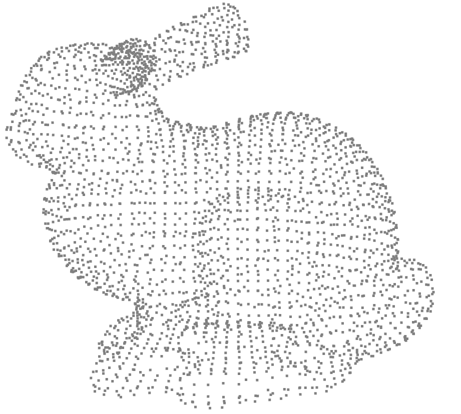
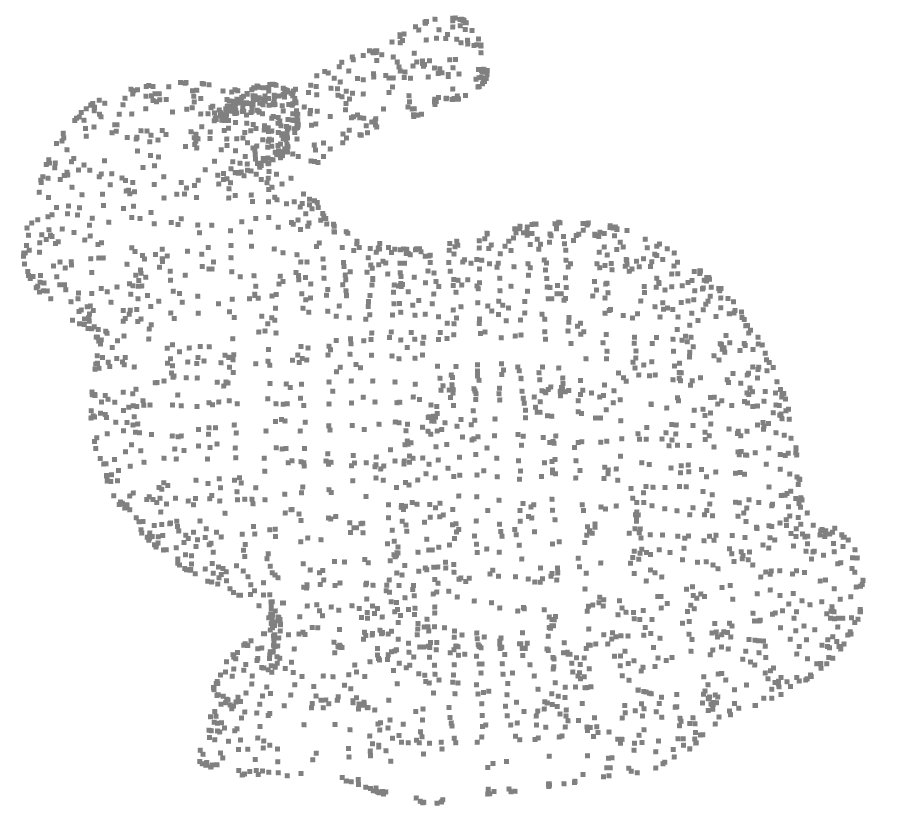
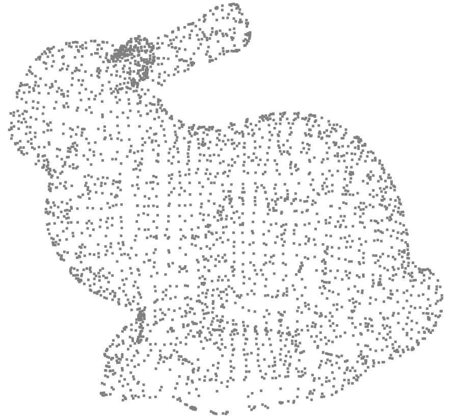
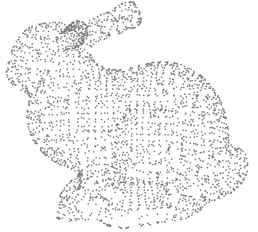
unseen
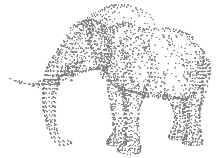
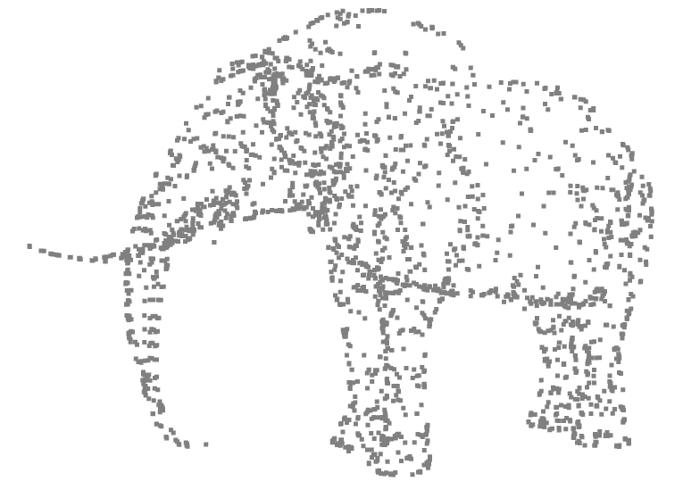
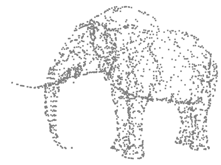
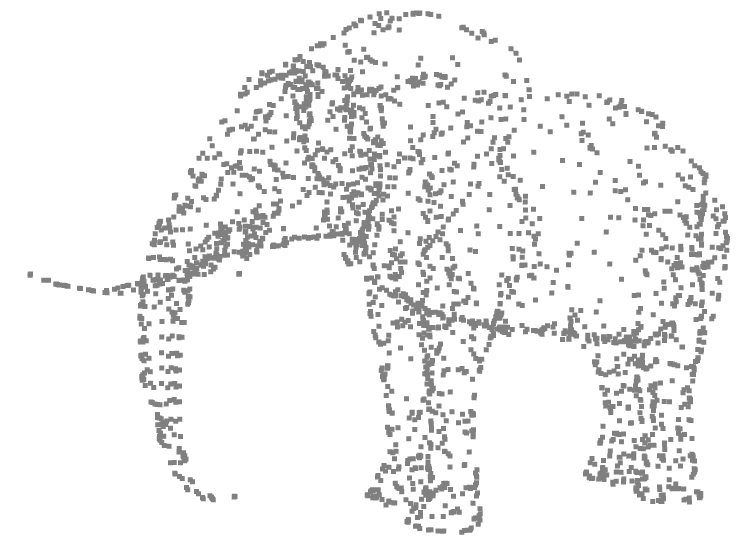
test

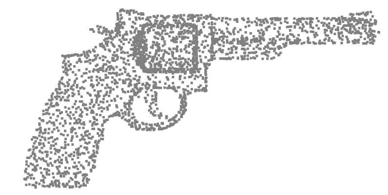
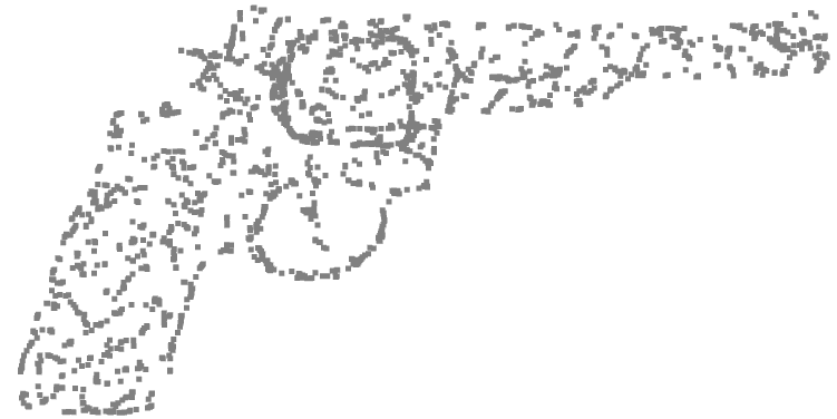
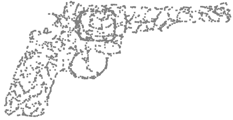
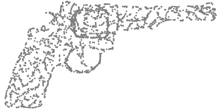
Figure 4: Comparison of NL-TV regularization (1) of point-clouds $X$ (for $p=2$, $q=1$, $\lambda=0.05$) with the MPN algorithm mpn-pd and trained GNN, using model distillation (8) or the unsupervised setting with variational optimization (7). Input here is either unseen point-clouds during training, or from the test category, hold out during training.

Training set	Validation set	Test set

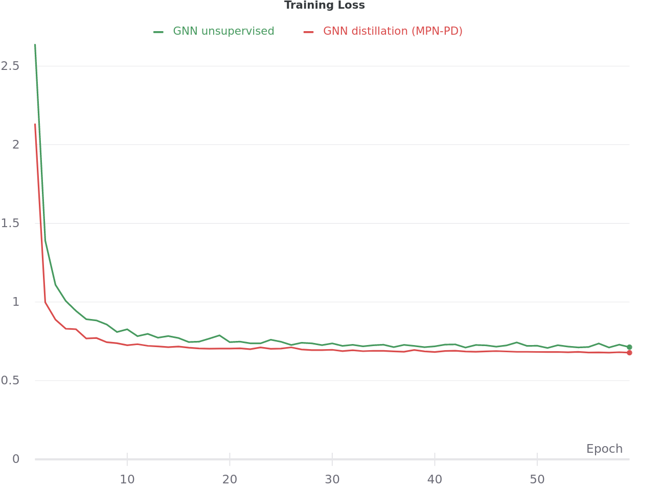
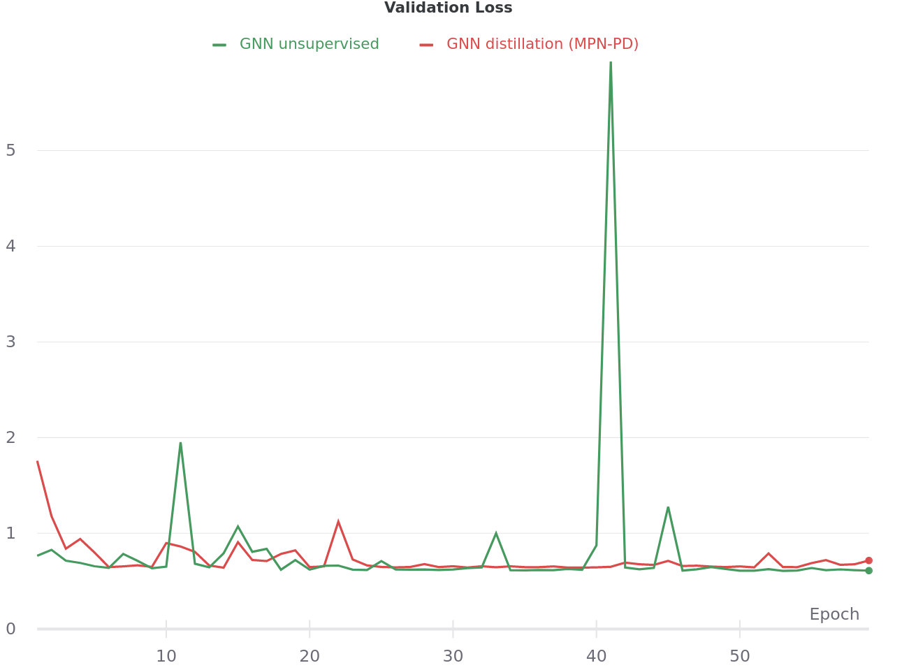
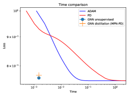
Figure 5: (left) Objective loss function (7) during GNN training versus epochs for the training and the validation sets. (right) Comparison of the average objective function $J$ in logarithmic scale versus average computation time for GNN, adam and mpn-pd.

Acknowledgments This work has been carried out with financial support from the French Research Agency through the SUMUM project (ANR-17-CE38-0004)

References

- [1] Bertocchi, C., Chouzenoux, E., Corbineau, M.C., Pesquet, J.C., Prato, M.: Deep unfolding of a proximal interior point method for image restoration. Inverse Problems 36(3), 034005 (2020)
- [2] Bruna, J., Zaremba, W., Szlam, A., LeCun, Y.: Spectral networks and locally connected networks on graphs. In: Int. Conf. on Learning Representations (2014)
- [3] Chambolle, A., Pock, T.: A first-order primal-dual algorithm for convex problems with applications to imaging. Journal of mathematical imaging and vision 40(1), 120–145 (2011)
- [4] Combettes, P.L., Pesquet, J.C.: Deep neural network structures solving variational inequalities. Set-Valued and Variational Analysis pp. 1–28 (2020)
- [5] Defferrard, M., Bresson, X., Vandergheynst, P.: Convolutional neural networks on graphs with fast localized spectral filtering. In: Advances in neural information processing systems. pp. 3844–3852 (2016)
- [6] Elmoataz, A., Lezoray, O., Bougleux, S.: Nonlocal discrete regularization on weighted graphs: a framework for image and manifold processing. IEEE Transactions on Image Processing 17(7), 1047–1060 (2008)
- [7] Elmoataz, A., Toutain, M., Tenbrinck, D.: On the -laplacian and -laplacian on graphs with applications in image and data processing. SIAM Journal on Imaging Sciences 8(4), 2412–2451 (2015)
- [8] Fey, M., Lenssen, J.E.: Fast graph representation learning with pytorch geometric. arXiv preprint arXiv:1903.02428 (2019)
- [9] Gilboa, G., Osher, S.: Nonlocal operators with applications to image processing. Multiscale Modeling & Simulation 7(3), 1005–1028 (2009)
- [10] Gilmer, J., Schoenholz, S.S., Riley, P.F., Vinyals, O., Dahl, G.E.: Neural message passing for quantum chemistry. In: ICML (2017)
- [11] Hasannasab, M., Hertrich, J., Neumayer, S., Plonka, G., Setzer, S., Steidl, G.: Parseval proximal neural networks. Journal of Fourier Analysis and Applications 26(4), 1–31 (2020)
- [12] Hidane, M., Lézoray, O., Elmoataz, A.: Nonlinear multilayered representation of graph-signals. Journal of mathematical imaging and vision 45(2), 114–137 (2013)
- [13] Kingma, D.P., Ba, J.: Adam: A method for stochastic optimization. In: Proceedings of the 3rd International Conference on Learning Representations (ICLR) (2014)
- [14] Kipf, T.N., Welling, M.: Semi-supervised classification with graph convolutional networks. In: Int. Conf. on Learning Representations (2017)
- [15] Kobler, E., Klatzer, T., Hammernik, K., Pock, T.: Variational networks: connecting variational methods and deep learning. In: German conference on pattern recognition. pp. 281–293. Springer (2017)
- [16] Li, R., Li, X., Fu, C.W., Cohen-Or, D., Heng, P.A.: Pu-gan: a point cloud upsampling adversarial network. In: Proceedings of the IEEE/CVF International Conference on Computer Vision. pp. 7203–7212 (2019)
- [17] Liu, D.C., Nocedal, J.: On the limited memory bfgs method for large scale optimization. Mathematical programming 45(1), 503–528 (1989)
- [18] Lozes, F., Hidane, M., Elmoataz, A., Lézoray, O.: Nonlocal segmentation of point clouds with graphs. In: 2013 IEEE Global Conference on Signal and Information Processing. pp. 459–462. IEEE (2013)
- [19] Meinhardt, T., Moller, M., Hazirbas, C., Cremers, D.: Learning proximal operators: Using denoising networks for regularizing inverse imaging problems. In: Proceedings of the IEEE ICCV. pp. 1781–1790 (2017)
- [20] Peyré, G., Bougleux, S., Cohen, L.: Non-local regularization of inverse problems. Inverse Problems & Imaging 5(2), 511 (2011)
- [21] Qi, C.R., Su, H., Mo, K., Guibas, L.J.: Pointnet: Deep learning on point sets for 3d classification and segmentation. In: Proceedings of the IEEE conference on computer vision and pattern recognition. pp. 652–660 (2017)
- [22] Qi, C.R., Yi, L., Su, H., Guibas, L.J.: Pointnet++: Deep hierarchical feature learning on point sets in a metric space. In: Advances in Neural Information Processing Systems. vol. 30 (2017)
- [23] Raguet, H., Landrieu, L.: Preconditioning of a generalized forward-backward splitting and application to optimization on graphs. SIAM Journal on Imaging Sciences 8(4), 2706–2739 (2015)
- [24] Raguet, H., Landrieu, L.: Cut-pursuit algorithm for regularizing nonsmooth functionals with graph total variation. In: International Conference on Machine Learning. pp. 4247–4256 (2018)
- [25] Tabti, S., Rabin, J., Elmoataz, A.: Symmetric upwind scheme for discrete weighted total variation. In: IEEE International Conference on Acoustics, Speech and Signal Processing (ICASSP). pp. 1827–1831 (2018)
- [26] Tenbrinck, D., Gaede, F., Burger, M.: Variational graph methods for efficient point cloud sparsification. arXiv preprint arXiv:1903.02858 (2019)
- [27] Wang, Y., Solomon, J.M.: Deep closest point: Learning representations for point cloud registration. In: Proceedings of the IEEE International Conference on Computer Vision. pp. 3523–3532 (2019)
- [28] Wang, Y., Sun, Y., Liu, Z., Sarma, S.E., Bronstein, M.M., Solomon, J.M.: Dynamic graph cnn for learning on point clouds. ACM Transactions On Graphics (TOG) 38(5), 1–12 (2019)
- [29] Williams, F., Schneider, T., Silva, C., Zorin, D., Bruna, J., Panozzo, D.: Deep geometric prior for surface reconstruction. In: Proceedings of the IEEE Conference on Computer Vision and Pattern Recognition. pp. 10130–10139 (2019)
- [30] Wu, F., Souza, A., Zhang, T., Fifty, C., Yu, T., Weinberger, K.: Simplifying graph convolutional networks. In: Proceedings of the 36th International Conference on Machine Learning. vol. 97, pp. 6861–6871. PMLR (2019)
- [31] Yang, G., Huang, X., Hao, Z., Liu, M.Y., Belongie, S., Hariharan, B.: Pointflow: 3d point cloud generation with continuous normalizing flows. In: Proceedings of the IEEE International Conference on Computer Vision. pp. 4541–4550 (2019)
- [32] Yi, L., Kim, V.G., Ceylan, D., Shen, I.C., Yan, M., Su, H., Lu, C., Huang, Q., Sheffer, A., Guibas, L.: A scalable active framework for region annotation in 3d shape collections. ACM Transactions on Graphics (ToG) 35(6), 1–12 (2016)