Fast Model-based Clustering of Partial Records

Abstract

Partially recorded data are frequently encountered in many applications and usually clustered by first removing incomplete cases or features with missing values, or by imputing missing values, followed by application of a clustering algorithm to the resulting altered dataset. Here, we develop clustering methodology through a model-based approach using the marginal density for the observed values, assuming a finite mixture model of multivariate $t$ distributions. We compare our approximate algorithm to the corresponding full expectation-maximization (EM) approach that considers the missing values in the incomplete dataset and makes a missing at random (MAR) assumption, as well as case deletion and imputation methods. Since only the observed values are utilized, our approach is computationally more efficient than imputation or full EM. Simulation studies demonstrate that our approach has favorable recovery of the true cluster partition compared to case deletion and imputation under various missingness mechanisms, and is at least competitive with the full EM approach, even when MAR assumptions are violated. Our methodology is demonstrated on a problem of clustering gamma-ray bursts and is implemented at https://github.com/emilygoren/MixtClust.

I Introduction

Cluster analysis partitions data into groups of similar observations in an unsupervised manner and commonly without knowledge of the total number of clusters. Clustering applications appear in many fields, including medical imaging [1], gene expression [2], microbiome studies [3], crime analysis [4], and astronomy [5]. Prominent approaches to cluster analysis can be grouped into centroid-based methods such as $k$-means [6], hierarchical clustering [7], and model-based methods [8]. Refer to [9, 10, 11, 8, 12, 13] for a comprehensive introduction to the rich topic of clustering.

In practice, real datasets may have missing values or otherwise partially observed records that complicate the validity and application of standard statistical methodology. Missingness may result from diverse causes, with an underlying mechanism of one of three types: missing completely at random (MCAR), missing at random (MAR), or not missing at random (NMAR) [14]. Under MCAR, the probability that a case (record, sample, or observation) is missing feature (variable, attribute, dimension) values does not depend on either the observed or missing feature values. The mechanism is MAR when this probability depends on the observed feature values, but not the missing feature values, and NMAR when the probability depends on both observed and missing feature values. Notably, MCAR data are also MAR; if the data are not MAR, then they are NMAR. Strategies for analysis of data with missing values are often critically dependent on the missingness mechanism, and clustering is no exception.

For clustering problems, the most common (and often expedient) treatment of missing values is deletion, on either a case or feature basis, or imputation [15, 16]. Given a dataset with $n$ cases and $p$ features, case deletion removes all cases with any missing values across the $p$ features, leading to a reduced dataset with $n^{\prime}<n$ cases that are fully observed for all the $p$ original features. After a clustering algorithm has been applied to the resulting reduced dataset of complete cases, the remaining $n-n^{\prime}$ incomplete cases can be assigned to the obtained cluster partition, for example, by using a partial distance [17] or marginal posterior probability [18] approach. An alternative deletion approach is executed on a feature-wise basis by discarding any features that are not observed for all $n$ cases, resulting in a dataset of $n$ cases but $p^{\prime}<p$ features, on which a clustering algorithm can be applied to directly cluster all cases [19]. While attractive for their ease of implementation, both data exclusion schemes make an assumption of a MCAR mechanism, violation of which leads to reduced clustering performance. Even if data are MCAR, deletion may yield poor clustering performance due to loss of information. In contrast, imputation approaches [20, 21, 22, 23] for clustering replace each missing value with a predicted value to produce a completed dataset that can be supplied to the desired algorithm to cluster all $n$ cases. Critically, this approach treats the imputed values as if they were observed values, and thus ignores any error and uncertainty associated with the fact that they are not the actual values. Obtaining a suitable method for imputation can be difficult because the most appropriate choice likely depends on the unknown cluster partition. As a consequence, use of imputation has been shown to substantially diminish clustering performance [16].

The drawbacks of deletion and imputation have prompted clustering approaches that incorporate the missing data structure, yet use all the observed entries in the dataset. [24] and [25] used a partial distance to measure the distance between differentially observed cases. [26] extended the fuzzy $k$-means algorithm for incomplete cases but after imposing soft constraints based on estimating the distance between incomplete cases and cluster centers. In fuzzy clustering, [27, 28, 29] utilized complete cases to define cluster centers and weights and multiply imputed the incomplete cases in the objective function. The $k$-means extension of [30] also used soft constraints defined by the partially observed features, but this requires at least one feature to be observed across all cases. The $k$-POD algorithm [31] employs majorization-minimization [32] to minimize the objective function of $k$-means using partial distances for incomplete cases. Recently, [33] developed the $k_{m}$-means algorithm, which generalized the $k$-means algorithm of [34] to include partially-observed records. These approaches all utilized the Euclidean metric for measuring the distance between observations and cluster centers, in the process assuming hyperspherical-shaped clusters and giving up on robustness to outliers.

Model-based clustering using finite mixtures of the multivariate Gaussian [35, 36] or $t$ distributions [37, 38] allow for hyperellipsoidal-shaped clusters [39] through use of the Mahalanobis distance [40] and have a long history of successful application. Compared to the Gaussian distribution, the $t$ distribution confers greater resistance to outliers through its wider tails, and is therefore often the de facto choice for model-based clustering. For clustering of incomplete data, [41] proposed finite mixture modeling using multivariate $t$ distributions and designed an expectation-maximization (EM) algorithm [42] for both estimating mixture model parameters and treatment of the missing values. [43] extended this work to incorporate the eigen-decomposed covariance structure of [35]. To better fit asymmetrical-shaped clusters, [44] developed an approach using skew-$t$ distributions while [45] extended this work with a eigen-decomposed covariance structure for skew-$t$-and generalized hyperbolic distributions. Importantly, all of these works included the missing values in the formal incomplete dataset within an EM algorithm. This may be computationally burdensome and lack robustness to the MAR assumption since, in the expectation step (E-step), the observed feature values inform those that are missing. When the data are NMAR, the observed values are not directly informative of those that are missing because their values are related to their own missingness.

In this paper, we (Section II) propose model-based clustering of partially recorded data using finite multivariate-$t$ mixture distributions for only the observed values by integrating out the missing values and excluding them from our clustering algorithm calculations. An alternating expectation-conditional maximization (AECM) algorithm [46] implements our approach and is seen in simulation studies (Section III) to reduce computational complexity when compared to a full EM approach and also to do well under violations of the MAR mechanism. Section IV uses our methodology to cluster gamma-ray bursts data. We conclude with some discussion in Section V. Two appendices have additional details.

II Methodology

II-A Background and Preliminaries

We begin by introducing our model and relevant notation for the problem of clustering the dataset $\bm{y}\in\mathbb{R}^{n\times p}$ consisting of $n$ cases and $p$ features into $K$ clusters, allowing for missing values in $\bm{y}$. For now, we treat $K$ as known, postponing discussion on choosing $K$ to later. Assume that the cases are independent and arise from a finite mixture of $t$ distributions described by the density $f(\bm{y}_{i}\>|\>\bm{\Theta})=\sum_{k=1}^{K}\pi_{k}t_{p}(\bm{y}_{i};~{}\bm{\mu}_{k},\bm{\Sigma}_{k},\nu_{k}),\quad i=1,\dots,n$ where $\pi_{k}\in(0,1)$ is the proportion represented by the $k^{th}$ cluster with $\sum_{k=1}^{K}\pi_{k}=1$, and $t_{p}(\cdot;\bm{\mu},\bm{\Sigma},\nu)$ is the $p$-variate $t$-density with mean $\bm{\mu}\in\mathbb{R}^{p}$, positive-definite real $p\times p$ dispersion matrix $\bm{\Sigma}$, and degrees of freedom $\nu>0$ defined as

$$t_{p}(\bm{y};\bm{\mu},\bm{\Sigma},\nu)=\frac{\Gamma\left(\frac{\nu+p}{2}\right)}{\Gamma\left(\frac{\nu}{2}\right)\nu^{\frac{p}{2}}\pi^{\frac{p}{2}}\lvert\bm{\Sigma}\rvert^{\frac{1}{2}}}\left[1+\frac{1}{\nu}\Delta(\bm{y},\bm{\mu},\bm{\Sigma})\right]^{-\frac{\nu+p}{2}},\quad\bm{y}\in\mathbb{R}^{p}$$ (1)

where $\Delta(\cdot)$ is the Mahalanobis distance [40] given by $\Delta(\bm{y},\bm{\mu},\bm{\Sigma})=(\bm{y}-\bm{\mu})^{\prime}\bm{\Sigma}^{-1}(\bm{y}-\bm{\mu}).$

In missing data problems, the $p$-dimensional records are only partially observed and we leverage the observed values for clustering. WLOG, suppose each $p$-vector is decomposed into observed and missing components as $\bm{y}_{i}=(\bm{y}_{i}^{o},\bm{y}_{i}^{m}),$ where $\bm{y}_{i}^{o}\in\mathbb{R}^{p_{i}^{o}}$ is the observed component and $\bm{y}_{i}^{m}\in\mathbb{R}^{p-p_{i}^{o}}$ is the missing component for each observation $i=1,\dots,n$. Define observed and missing component selection matrices $\bm{O}_{i}$ and $\bm{M}_{i}$, respectively, such that $\bm{O}_{i}$ extracts the observed component from $\bm{y}_{i}$ and has dimension $p_{i}^{o}\times p$, and $\bm{M}_{i}$, of dimension $(p-p_{i}^{o})\times p$, extracts the missing component from $\bm{y}_{i}$. Then $\bm{y}_{i}^{o}=\bm{O}_{i}\bm{y}_{i},\quad\bm{y}_{i}^{m}=\bm{M}_{i}\bm{y}_{i}.$These two matrices together account for the entire $p$-dimensional vector through the property $\bm{O}_{i}^{\prime}\bm{O}_{i}+\bm{M}_{i}^{\prime}\bm{M}_{i}=\bm{I}_{p}$. Omitting the vacuous case where no features are observed, there are $\sum_{l=0}^{p-1}{p\choose l}=2^{p}-1$ unique patterns of missingness possible for each case. The marginal density [47] of the observed values in the $i$th observation record is

$$f\left(\bm{y}_{i}^{o}\>|\>\bm{\Theta}\right)=\sum_{k=1}^{K}\pi_{k}t_{p_{i}^{o}}\left(\bm{y}_{i}^{o};~{}\bm{\mu}_{ik}^{o},\bm{\Sigma}_{ik}^{oo},\nu_{k}\right),\quad i=1,\dots,n$$ (2)

where $\bm{\mu}_{ik}^{o}=\bm{O}_{i}\bm{\mu}_{k}$ and $\bm{\Sigma}_{ik}^{oo}=\bm{O}_{i}\bm{\Sigma}_{k}\bm{O}_{i}^{\prime}$ are the mean and dispersion of the observed components of the $i$th record in the $k^{\text{th}}$ cluster.

Comment

Our development above uses $\bm{O}_{i}$ as a non-stochastic selection matrix to specify the presence of measurement for the $i$th record, and as a computational device. As pointed out by a reviewer, a more accurate development would involve incorporating the stochastic nature of $\bm{O}_{i}$ to capture the missingness mechanism if such were available. However, incorporating such a mechanism is application-specific, and so for this paper, we have assumed that the missingness mechanism is unavailable to us, and inherently MCAR.

II-B EM Algorithm for Parameter Estimation

II-B1 Complete data and log likelihood

A EM algorithm for parameter estimation can be formulated using (2) by specifying a so-called complete dataset and corresponding log likelihood. Since missing values are omitted in (2), the “actual” missing values $\{\bm{y}_{i}^{m}:i=1,\dots,n\}$ are not part of the complete dataset; instead we include the “conceptual” missing values of class memberships and characteristic weights that we now introduce. Finite mixture modeling approaches to clustering can be recast as a problem of missing cluster membership labels. To this end, we define the latent class membership indicators

$$z_{ik}=\mathbb{I}(\text{case $i$ belongs to class $k$}),\quad i=1,\dots,n;~{}k=1,\dots,K$$ (3)

where $\mathbb{I}(\cdot)$ denotes the indicator function. As an unsupervised learning task, all the $z_{ik}$’s are missing. To devise an EM algorithm, we also utilize the multivariate Gaussian-gamma mixture formulation of the multivariate $t$ distribution [48], rewriting (1) as

$$t_{p}(\bm{y};\bm{\mu},\bm{\Sigma},\nu)=\int_{0}^{\infty}\phi(\bm{y};\bm{\mu},\bm{\Sigma}/w)q(w;\nu/2,\nu/2)~{}\text{d}w,\quad\bm{y}\in\mathbb{R}^{p}$$ (4)

where $\phi(\bm{y};\bm{\mu},\bm{\Sigma}/w)={\lvert\bm{\Sigma}\rvert^{-\frac{1}{2}}\left(2\pi/w\right)^{-p/2}}\exp\left(-\frac{w}{2}\Delta(\bm{y},\bm{\mu},\bm{\Sigma})\right),\mbox{ for }\bm{y}\in\mathbb{R}^{p},$is the $p$-variate Gaussian distribution with mean $\bm{\mu}$ and variance $\bm{\Sigma}/w$ denoted by $\mathcal{N}_{p}\left(\bm{\mu},\bm{\Sigma}/w\right)$, and $q(w;\nu/2,\nu/2)=\{(\nu/2)^{\nu/2}/\Gamma(\nu/2)\}\exp\left(-\nu w/2\right)w^{\nu/2-1},\mbox{ for }w>0,$is the gamma distribution with shape and rate parameters both given by $\nu/2$, and denoted by $\text{Gamma}(\nu/2,\nu/2)$. The random variable $w$ can be understood as a latent characteristic weight. This provides a hierarchical specification of (2) that is defined by

$${\mathcal{L}}(\bm{y}_{i}^{o}\>|\>w_{i},z_{ik}=1)\equiv\mathcal{N}_{p_{i}^{o}}\left(\bm{O}_{i}\bm{\mu}_{k},\frac{1}{w_{i}}\bm{O}_{i}\bm{\Sigma}_{k}\bm{O}_{i}^{\prime}\right),\quad{\mathcal{L}}(w_{i}\>|\>z_{ik}=1)\equiv\text{Gamma}\left(\nu_{k}/2,\nu_{k}/2\right),\quad\bm{z}_{i}\sim\text{Multinomial}\left(1;\pi_{1},\dots,\pi_{K}\right)$$

where $\bm{z}_{i}=(z_{i1},\dots,z_{iK})^{\prime}$ is the vector of latent class labels and $w_{i}$ is the characteristic weight for the $i^{\text{th}}$ observation.

Together, we take $\{\bm{y}_{i}^{o},\bm{z}_{i},w_{i}:i=1,\dots,n\}$ to be the complete data, disregarding the missing values $\{\bm{y}_{i}^{m}:i=1,\dots,n\}$. The corresponding complete data log likelihood for the parameters $\bm{\Theta}$ is, but for an additive constant, given by

$$\ell_{c}\left(\bm{\Theta}\>|\>\bm{y}^{o},\bm{w},\bm{z}\right) =\sum_{i=1}^{n}\sum_{i=k}^{K}\Bigg{[}z_{ik}\log\pi_{k}+z_{ik}\log\mathcal{N}_{p_{i}^{o}}\left(\bm{y}_{i}^{o};~{}\bm{O}_{i}\bm{\mu}_{k},\frac{1}{w_{i}}\bm{O}_{i}\bm{\Sigma}_{k}\bm{O}_{i}^{\prime}\right)+z_{ik}\log\text{Gamma}\left(w_{i};~{}\nu_{k}/2,\nu_{k}/2\right)\bigg{]}$$

$$=\sum_{k=1}^{K}\sum_{i=1}^{n}\Bigg{[}z_{ik}\log\pi_{k}-\frac{z_{ik}}{2}\left(\log\lvert\bm{O}_{i}\bm{\Sigma}_{k}\bm{O}_{i}^{\prime}\rvert+w_{i}(\bm{y}_{i}-\bm{\mu}_{k})^{\prime}\bm{O}_{i}^{\prime}(\bm{O}_{i}\bm{\Sigma}_{k}\bm{O}_{i}^{\prime})^{-1}\bm{O}_{i}(\bm{y}_{i}-\bm{\mu}_{k})\right)$$

$$\hskip 56.9055pt+z_{ik}\left(\frac{\nu_{k}}{2}\log\left(\frac{\nu_{k}}{2}\right)-\log\Gamma\left(\frac{\nu_{k}}{2}\right)+\frac{\nu_{k}}{2}\left(\log w_{i}-w_{i}\right)\right)\bigg{]}.$$ (5)

II-B2 An AECM algorithm for parameter estimation

We now design an AECM algorithm for maximum likelihood estimation of all the model parameters $\bm{\Theta}=\{\bm{\mu}_{1},\bm{\Sigma}_{1},\nu_{1},\dots,\bm{\mu}_{K},\bm{\Sigma}_{K},\nu_{K}\}$ assuming the complete data log likelihood function in (5). The AECM approach differs from a general EM approach in that it breaks down each iteration by partitioning the parameter space into blocks, and cycles through the partition by alternating between updating each block of parameters through a conditional maximization (CM-step) and an E-step. For fully observed data, our approach reduces to that of [49] for unconstrained dispersion matrices.

The Q-function, given previous iteration parameter estimates $\hat{\bm{\Theta}}$, is $Q\left(\bm{\Theta}\>|\>\hat{\bm{\Theta}}\right)=\sum_{k=1}^{k}\bigg{[}Q_{1}\left(\pi_{k}\>|\>\hat{\bm{\Theta}}\right)+Q_{2}\left(\bm{\mu}_{k},\bm{\Sigma}_{k}\>|\>\hat{\bm{\Theta}}\right)+Q_{3}\left(\nu_{k}\>|\>\hat{\bm{\Theta}}\right)\bigg{]},$where (excluding constant terms) we have

$$Q_{1}\left(\pi_{k}\>|\>\hat{\bm{\Theta}}\right) =\sum_{i=1}^{n}\hat{z}_{ik}\log\pi_{k},$$

$$Q_{2}\left(\bm{\mu}_{k},\bm{\Sigma}_{k}\>|\>\hat{\bm{\Theta}}\right) =\sum_{i=1}^{n}\frac{\hat{z}_{ik}}{2}\bigg{[}-\log\lvert\bm{O}_{i}\bm{\Sigma}_{k}\bm{O}_{i}^{\prime}\rvert-\hat{w}_{ik}(\bm{y}_{i}-\bm{\mu}_{k})^{\prime}\bm{O}_{i}^{\prime}(\bm{O}_{i}\bm{\Sigma}_{k}\bm{O}_{i}^{\prime})^{-1}\bm{O}_{i}(\bm{y}_{i}-\bm{\mu}_{k})\bigg{]},$$

$$\mbox{ and }\qquad Q_{3}\left(\nu_{k}\>|\>\hat{\bm{\Theta}}\right) =\sum_{i=1}^{n}\hat{z}_{ik}\bigg{[}\frac{\nu_{k}}{2}\log\left(\frac{\nu_{k}}{2}\right)-\log\Gamma\left(\frac{\nu_{k}}{2}\right)+\frac{\nu_{k}}{2}\left\{\log\hat{w}_{ik}+\psi\left(\frac{\hat{\nu}_{k}+p_{i}^{o}}{2}\right)-\log\left(\frac{\hat{\nu}_{k}+p_{i}^{o}}{2}\right)-\hat{w}_{ik}\right\}\bigg{]},$$

with $\psi(\cdot)$ as the digamma function, $\hat{z}_{ik}$ as the (current iteration) posterior probability that the $i$th record belongs to cluster $k$, and $\hat{w}_{ik}$ is the (current iteration) conditional expectation of $w_{i}$ given $\bm{y}_{i}^{o}$ and $z_{ij}=1$. The later weights the influence of $\bm{y}_{i}^{o}$ in estimation of $\bm{\mu}_{k}$ and $\bm{\Sigma}_{k}$.

In the E-step, given current parameter estimates $\hat{\bm{\Theta}}$, we obtain the updates

$$\hat{z}_{ik} \equiv\operatorname{E}_{\hat{\bm{\Theta}}}\left(z_{ik}\>|\>\bm{y}_{i}^{o}\right)=\frac{\hat{\pi}_{k}t_{p_{i}^{o}}\left(\bm{y}_{i}^{o};~{}\bm{O}_{i}\hat{\bm{\mu}}_{k},\bm{O}_{i}\hat{\bm{\Sigma}}_{k}\bm{O}_{i}^{\prime},\hat{\nu}_{k}\right)}{\sum_{k^{\prime}=1}^{K}\hat{\pi}_{k^{\prime}}t_{p_{i}^{o}}\left(\bm{y}_{i}^{o};~{}\bm{O}_{i}\hat{\bm{\mu}}_{k^{\prime}},\bm{O}_{i}\hat{\bm{\Sigma}}_{k^{\prime}}\bm{O}_{i}^{\prime},\hat{\nu}_{k^{\prime}}\right)},\quad\mbox{ and }$$

$$\hat{w}_{ik}\equiv \operatorname{E}_{\hat{\bm{\Theta}}}\left(w_{i}\>|\>\bm{y}_{i}^{o},z_{ik}=1\right)=\frac{\hat{\nu}_{k}+p_{i}^{o}}{\hat{\nu}_{k}+(\bm{y}_{i}-\hat{\bm{\mu}}_{k})^{\prime}\bm{O}_{i}^{\prime}(\bm{O}_{i}\hat{\bm{\Sigma}}_{k}\bm{O}_{i}^{\prime})^{-1}\bm{O}_{i}(\bm{y}_{i}-\hat{\bm{\mu}}_{k})}.$$

To define the CM-steps, we form the parameter space partition $\bm{\Theta}=\big{\{}\{\pi_{1},\bm{\mu}_{1},\nu_{1}\dots,\pi_{K},\bm{\mu}_{K},\nu_{K}\},~{}\{\bm{\Sigma}_{1},\dots,\bm{\Sigma}_{K}\}\big{\}}$ following [50]. Our computation in the CM-steps makes use of missingness indicator vectors

$$\bm{a}_{i}=\big{[}\mathbb{I}(y_{i1}\text{ is observed}),\dots,\mathbb{I}(y_{ip}\text{ is observed})\big{]}^{\prime}$$

defined for $i=1,\dots,n$. In the first CM-step, we update the $\pi_{k}$’s according to $\hat{\pi}_{k}={\sum_{i=1}^{n}\hat{z}_{ik}}/{n}$, where the numerator $\sum_{i=1}^{n}\hat{z}_{ik}$ can be understood as representing an estimated (current iteration) sample size from the $k$th group. Also in the first CM-step, for computational simplicity, we can update the $\bm{\mu}_{k}$s, following derivations in Appendix A, by

$$\hat{\bm{\mu}}_{k}=\left(\sum_{i=1}^{n}\hat{z}_{ik}\hat{w}_{ik}\operatorname{diag}(\bm{a}_{i})\right)^{-1}\sum_{i=1}^{n}\hat{z}_{ik}\hat{w}_{ik}\operatorname{diag}(\bm{a}_{i})\bm{y}_{i},$$ (6)

if it increases $Q_{2}(\cdot)$, or we keep the current value (however, see the comment below). Compared to updates for $\bm{\mu}_{k}$ using fully observed data, the missingness indicators $\bm{a}_{i}$ in the RHS of (6) only add element-wise contributions for observed values. Similarly, the LHS term serves as an element-wise number-of-observations adjustment for the number of observed values in each feature. The first CM-step then updates the $\nu_{k}$s as the solution to

$$1+\log\left(\frac{\nu_{k}}{2}\right)+1-\psi\left(\frac{\nu_{k}}{2}\right)+\frac{1}{\sum_{i=1}^{n}\hat{z}_{ik}}\sum_{i=1}^{n}\hat{z}_{ik}\bigg{[}\log\hat{w}_{ik}+\psi\left(\frac{\hat{\nu}_{k}+p_{i}^{o}}{2}\right)-\log\left(\frac{\hat{\nu}_{k}+p_{i}^{o}}{2}\right)-\hat{w}_{ik}\bigg{]}=0.$$ (7)

There is no closed-form solution to (7). Our R package MixtClust offers a numerical solution using Brent’s method [51] and, by default, also extends the closed-form approximation introduced by [49] that uses

$$\hat{\nu}_{k}\approx\frac{-\exp(v_{k})+2\exp(v_{k})\left[\exp\left(\psi\left(\frac{\hat{\nu}_{k}^{\text{old}}}{2}\right)\right)-\frac{\hat{\nu}_{k}^{\text{old}}}{2}+\frac{1}{2}\right]}{1-\exp(v_{k})},$$

by modifying $v_{k}$ to only use the observed number of features $p_{i}$, in contrast to $p$, for the $i^{\text{th}}$ observation:

$$v_{k}=-1-\frac{1}{\sum_{i=1}^{n}\hat{z}_{ik}}\sum_{i=1}^{n}\left[\hat{z}_{ik}(\log\hat{w}_{ik}-\hat{w}_{ik})-\psi\left(\frac{\hat{\nu}^{\text{old}}_{k}+p_{i}}{2}\right)+\log\left(\frac{\hat{\nu}^{\text{old}}_{k}+p_{i}}{2}\right)\right].$$

The second CM-step updates (see Appendix A for derivations and explanations), also for computational reasons, suggests updating $\bm{\Sigma}_{k}$’s as

$$\hat{\bm{\Sigma}}_{k}=\left(\sum_{i=1}^{n}\hat{z}_{ik}\bm{a}_{i}\bm{a}_{i}^{\prime}\right)^{\odot-1}\odot\left(\sum_{i=1}^{n}\hat{z}_{ik}\hat{w}_{ik}\operatorname{diag}(\bm{a}_{i})(\bm{y}_{i}-\hat{\bm{\mu}}_{k})(\bm{y}_{i}-\hat{\bm{\mu}}_{k})^{\prime}\operatorname{diag}(\bm{a}_{i})\right),$$ (8)

if $Q_{2}(\cdot)$ is increased, or we keep the current value for $\hat{\Sigma}_{k}$ (see, as before, the comment below). where $(\cdot)^{\odot-1}$ denotes Hadamard (element-wise) inverse, $\odot$ denotes Hadamard product, and $\otimes$ denotes tensor product. The missingness indicators play similar roles as with $\bm{\mu}_{k}$s, but here they operate on the elements of a $p\times p$ matrix rather than a $p$-vector. Our suggested updates therefore provide for a generalized EM algorithm [42, 52].

Comment

The check for the $Q_{2}(\cdot)$ at each of the two CM steps can be quite expensive, so our implementation instead checks for an increase in the loglikelihood at each cycle, terminating the algorithm at the previous iteration if there is a reduction in the total loglikelihood. The calculation of the loglikelihood is needed to be made at each cycle to assess convergence, so does not increase computational cost.

Comparison to full EM

Our approach uses marginalization, therefore excluding consideration of the missing data values $\bm{y}_{1}^{m},\dots,\bm{y}_{n}^{m}$ in the formulation of the incomplete dataset for EM style algorithms and so does not utilize the distribution of missing values conditional on the observed values, i.e., $f\left(\bm{y}_{i}^{m}\>|\>\bm{y}_{i}^{o},\bm{\Theta}\right)$, which contrasts to the approach of [43]. While their approach uses a different parameter space partition, the primary difference is that their CM-step updates for $\bm{\mu}_{k}$ and (general covariance structure) $\bm{\Sigma}_{k}$ replaces (6) and (8) by

$$\hat{\bm{\mu}}_{k}=\frac{\sum_{i=1}^{n}\hat{z}_{ik}\hat{w}_{ik}\hat{\bm{y}}_{ik}}{\sum_{i=1}^{n}\hat{z}_{ik}\hat{w}_{ik}},\qquad\mbox{and}\qquad\hat{\bm{\Sigma}}_{k}=\frac{\sum_{i=1}^{n}\hat{\bm{\Omega}}_{ik}}{\sum_{i=1}^{n}\hat{z}_{ik}}$$

where

$$\hat{\bm{y}}_{ik} \equiv\operatorname{E}_{\hat{\bm{\Theta}}}\left(\bm{y}_{i}\>|\>\bm{y}_{i}^{o},w_{i},z_{ik}=1\right)=\hat{\bm{\mu}}_{k}+\hat{\bm{\Sigma}}_{k}\bm{O}_{i}^{\prime}(\bm{O}_{i}\hat{\bm{\Sigma}}_{k}\bm{O}_{i}^{\prime})^{-1}\bm{O}_{i}(\bm{y}_{i}-\hat{\bm{\mu}}_{k})$$ (9)

$$\hat{\bm{\Omega}}_{ik} \equiv\operatorname{E}_{\hat{\bm{\Theta}}}\left(z_{ik}w_{i}(\bm{y}_{i}-\bm{\mu}_{k})(\bm{y}_{i}-\bm{\mu}_{k})^{\prime}\>|\>\bm{y}_{i}^{o}\right)=\hat{z}_{ik}\left[\hat{w}_{ik}(\hat{\bm{y}}_{ik}-\hat{\bm{\mu}}_{k})(\hat{\bm{y}}_{ik}-\hat{\bm{\mu}}_{k})^{\prime}+\big{(}\bm{I}_{p}-\hat{\bm{\Sigma}}_{k}\bm{O}_{i}^{\prime}(\bm{O}_{i}\hat{\bm{\Sigma}}_{k}\bm{O}_{i}^{\prime})^{-1}\bm{O}_{i}\big{)}\hat{\bm{\Sigma}}_{k}\right]$$ (10)

are updated in the E-step. Our approach only performs computations on the $\sum_{i=1}^{n}\sum_{j=1}^{p}a_{ij}\leq np$ observed values in the dataset, rather than on all $np$ values, in the updates for the $\bm{\mu}_{k}$’s and $\bm{\Sigma}_{k}$’s in this full EM approach. We also avoid computing  (9) and (10) altogether, which in the full EM approach need to be updated between every CM-step. While imputation approaches also avoid evaluating the equations, they perform computations on $np$ values. Therefore, our method by design has fewer computations and is faster than all comparative methods that account for missing values. However, our algorithm is also prone to premature termination, with effects that we account for in the next section.

II-B3 Initialization and convergence assessment

EM algorithms and their variants such as AECM find solutions in the vicinity of their initialization, with convergence leading to the discovery of a local, but not necessarily global, solution. Consequently, good starting values are important for its good performance. [53] provided the em-EM algorithm that runs the EM algorithm (“em” or “short EM”) from multiple starting points to lax convergence and then chooses the solution with the highest loglikelihood and runs the EM algorithm to strict convergence. A modification [54] proposes eschewing the potentially expensive loglikelihood check at each “em” step, running each “em” attempt for a small fixed number of iterations, and then runs the top few ones with highest loglikelihood for the long run and then choosing the one that upon convergence the estimate produces the largest log likelihood. We use this “Modified em-EM” approach [54] in our AECM algorithm for the full EM computations, with $K\sqrt{np}$ short runs and 10 long runs. However, our marginalization approach does not guarantee increases in the loglikelihood, so we adopt the Rnd-EM algorithm of [55], that eliminates the “em” steps altogether. We address the case of premature termination by having a large number (here, 10, to allow for fair comparison across methods, but perhaps much more) of long runs. We choose the initial seeds in the same manner as [33] and follow with one run of the EM cycle. Beyond checking for decreases in the loglikelihood (for the marginalization case), we use a lack-of-progress criterion to assess algorithm convergence, stopping when $\ell\big{(}\hat{\bm{\Theta}}^{(t+1)}\big{)}-\ell\big{(}\hat{\bm{\Theta}}^{(t)}\big{)}<\varepsilon$ for a desired small $\varepsilon>0$ (we use $\varepsilon=0.001$), where $\ell$ is the observed-data log likelihood resulting from (2) and $\hat{\bm{\Theta}}^{(t)}$ is the estimate of $\bm{\Theta}$ at the $t^{\text{th}}$ AECM iteration.

II-C Determining the number of clusters

The AECM algorithm presented here assumes a known $K$ or number of clusters. However, this is rarely the case in applications, and we precede by formulating the choice of $K$ as a model selection problem. Commonly, the Bayesian information criterion (BIC) [56] is used to discriminate between competing models for a given dataset, and is defined by $\text{BIC}=-2\ell\big{(}\hat{\bm{\Theta}}\big{)}+m\log n,$ where $\ell\big{(}\hat{\bm{\Theta}}\big{)}$ is the maximized observed-data log likelihood and $m$ is the number of free parameters to be estimated. We choose $K$ by choosing, from among a range of candidate values, the one attaining the smallest BIC at convergence. This approach of using BIC to determine the number of clusters in finite mixture models is well-established (see, e.g. [57, 58, 8]).

III Performance Assessment

This section reports performance evaluations in simulation experiments of our methodology relative to competing methods.

III-A Simulation study design

We simulated data with varying clustering complexities determined by the generalized overlap of and maximum eccentricity of [59] and implemented in the R package MixSim [60]. The generalized overlap [61], denoted here by $\mathring{\omega}$, adopted ideas from [62] to arrive at a one-point measure of clustering complexity, specifically, a numerical summary of the overall overlap between pairs of clusters. Higher values of the generalized overlap correspond to increased cluster overlap and consequently higher clustering complexity. Eccentricity controls the shape of the clusters, and is specified as $e=\sqrt{1-d_{\min}/d_{\max}}$, where $d_{\min}$ and $d_{\max}$ correspond to the smallest and largest eigenvalues of the dispersion matrix. Taking values in $[0,1]$, a perfect hypersphere has eccentricity $e=0$ whereas a perfect hyperplane has eccentricity $e=1$. Our simulations considered two clustering complexities: low ($\mathring{\omega}=0.001,e=0.5$) and high ($\mathring{\omega}=0.01,e=0.9$). For each complexity level, we simulated 100 complete datasets with $p=3$ features, $K=3$ clusters, $n=100$ cases. The degrees of freedom were set to be $\nu_{k}=15$ for all three clusters in our simulation experiments.

Given each full synthetic dataset, we deleted values according to the MCAR, MAR, NMAR1, and NMAR2 mechanisms to produce partially recorded datasets for comparing the competing clustering algorithms. For the MCAR setting, we randomly removed $\lambda np$ values across the entire dataset so that each element $y_{ij}$ had the same probability of being missing for $i=1,\dots,n$ and $j=1,\dots,p$. Under MAR, we randomly removed $\lambda np$ values in only the first two features according to MCAR, as in [31]. Our experiments considered two versions of NMAR. The NMAR1 version of [33] had one cluster being fully observed with the other two clusters having MCAR observations. The NMAR2 version [31, 33] also had one cluster fully observed, but the other clusters have the appropriate bottom quantile of each feature removed so as to achieve an overall missingness level $\lambda$. Figure 1 represents a sample dataset in the high clustering complexity scenario with the four patterns of missingness, for $\lambda=0.1$. (For our experimental evaluations, we ensured that there were at least $(p+1)$ complete records from each cluster, to allow for methods such as deletion to work.) For the first set of experiments, where our comparisons also included imputation methods, we set $\lambda=0.1$. For the more thorough, comprehensive

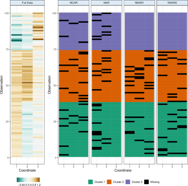
Figure 1: Representative sample simulated three-dimensional dataset in a high clustering complexity scenario. The leftmost figure is the heatmap of a MixSim-simulated three-groups full dataset before observations were deleted. The right panel of figures provides the corresponding observation status (either missing, or if observed, cluster membership) of each observation in the four missingness mechanisms (MAR, MCAR, NMAR1, NMAR2).

evaluations that only considered model-based clustering methods, we used $\lambda\in\{0.05,0.1,0.15,0.2\}$, as well as samples of $n=50$ and $n=100$ observations. The smaller sample size was chosen to provide us with a sense of performance when the average number of observations per cluster was not particularly high relative to dimension. This translated to between 10-16%, 20-32%, 26-46% and 34-57% of observations in our simulated datasets having at least one incomplete record.

III-B Comparison methods and evaluation

From now on, for ease of reference, we label our proposed approach as “Observed EM”, the full EM approach as “Full EM” and the case deletion approach, that only makes use of complete cases, as “Complete Case.” We also consider three imputation schemes to produce completed datasets before applying our software: Amelia II, mi, and mice. The Amelia II approach of [22] assumes the data are multivariate Gaussian and combines the EM algorithm with bootstrapping to draw from the posterior of the complete data parameters that are then used for imputation. In contrast, the mice and mi methods of [20] and [63], respectively, make use of chained equations to impute missing values. For all imputation approaches, we used default settings to generate $M=5$ completed datasets and performed clustering using the average of the $M$ imputed values. We evaluated clustering performance by comparing the the true cluster partition to that obtained by each method at the BIC-determined best $K$ (from now on denoted by $\hat{K}$) via the Adjusted Rand index (ARI) [64]. The (unadjusted) Rand index [65] is a measure of class agreement taking value in $[0,1]$, with a value of one indicating perfect agreement. Under random classification, the Rand index has an expected value greater than zero, reflecting the fact that, by chance alone, random classification could correctly classify some observations. The ARI [64] is a modification of the Rand index that, in contrast, has expected value of zero under random classification while retaining the property that a value of one corresponds to perfect classification.

III-C Simulation results

III-C1 Clustering performance

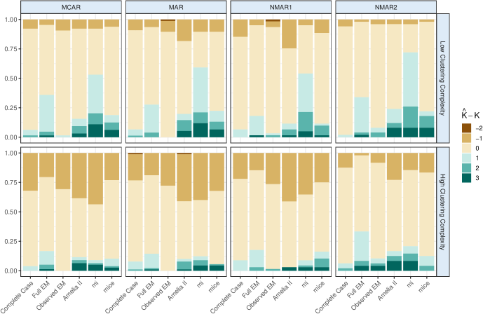
(a) Recovery of true $K$

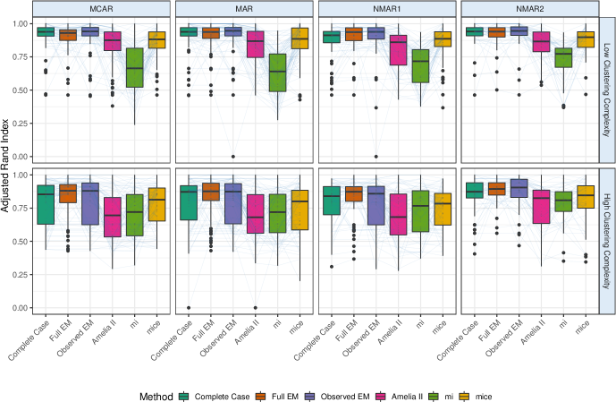
(b) Clustering performance of competing methods, as per ARI

Figure 2: Simulation results across 100 simulation replications for each method, missingness mechanism, and clustering complexity scenario. (a) accuracy of BIC in recovering the true number of clusters demonstrated in terms of the difference between the number of clusters chosen by BIC $\hat{K}$, and the true $K$. (b) ARI values comparing the true partition to the clustering obtained at $\hat{K}$.

We evaluate our clustering methods in terms of $K$-selection and in terms of the ability of our methods to obtain the true partition. Figure 2 displays a summary of our results. We consider accuracy of BIC in selecting the number of clusters in Figure 2a. Under high clustering complexity, most algorithms tended to select too few, rather than too many, clusters. However, in general, and except for being edged out by the “Complete Case” in NMAR2 for both clustering complexity situations and MAR for the low clustering complexity scenario, our “Observed EM” algorithm usually deviated the least from the true $K$. All three imputation methods generally selected more than the true $K$, and this was exaggerated under low clustering complexity. Within each pattern of missingness and clustering complexity, “Observed EM” provided competitive recovery of the true $K$. The cluster partition at $\hat{K}$ was next compared to the true class memberships using the ARI, and is summarized in Figure 2b. Overall, our approach produced cluster partitions at least as, or more, closely aligned with the truth under low clustering complexity for all missingness mechanisms. On the other hand, for high clustering complexity problems, our method is only the best overall under NMAR2, and for the remaining three missingness mechanisms for which the MAR assumption holds or is not as severely violated, our approach is only surpassed by “Full EM”.

The results of our simulation experiments show good performance of our “Observed EM” procedure. In cases with high clustering complexity, “Full EM” performs better than our case. However, even here, “Observed EM” is quite competitive. We now evaluate both methods against each other and “Complete Case” in a more comprehensive set of experiments.

III-C2 Comprehensive comparisons between “Observed EM”, “Full EM” and “Complete Case” methods

Evaluations at the true $K$

Our first set of evaluations assumed that the true $K$ was known.

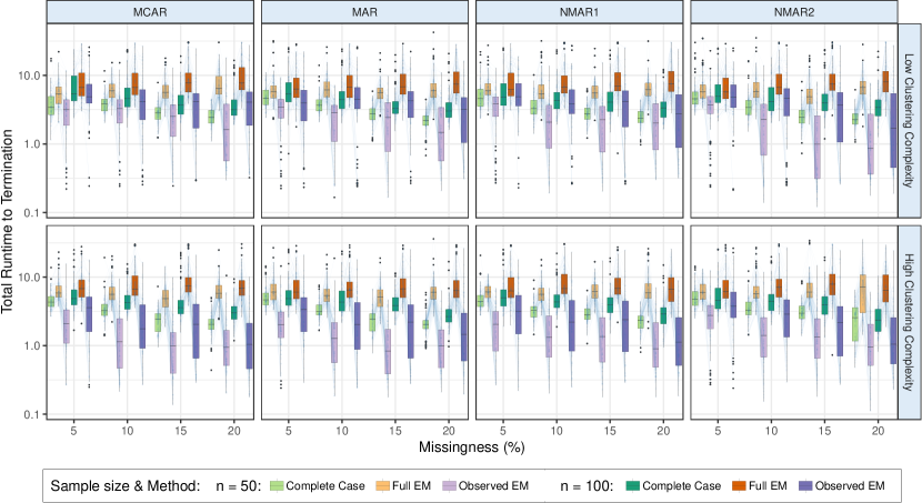
(a) Time to Termination of the three EM algorithms

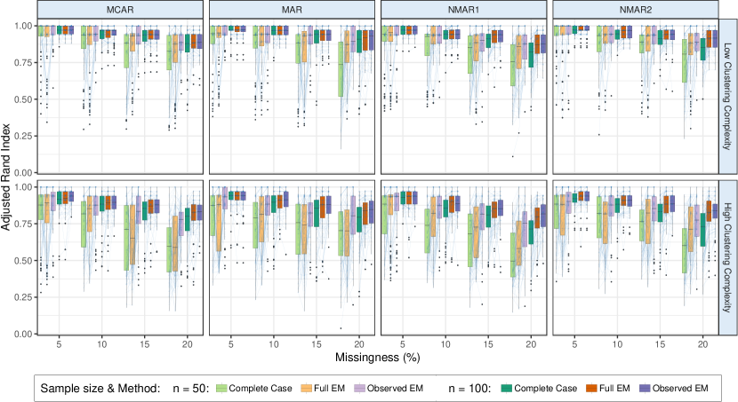
(b) Clustering performance of competing methods, as per ARI

Figure 3: Comprehensive simulation results at the known true $K$

We report performance for the three mehods in Figure 3. The discussion at the end of Section II-B2 demonstrated that the number of calculations needed to conduct one iteration of our “Observed EM” approach is no more (and often much less) than those needed for “Full EM”. However, because the trajectories taken by the two methods can be different, we also evaluated the runtime of each algorithm. Figure 3a shows that the time taken to termination is almost always smaller for the “Observed EM” case as opposed to the “Full EM” case, and this advantage increases with higher clustering complexity and amounts of missingness. (Interestingly, the “Complete Case” is slower than “Observed EM” despite its computations being often done on substantially smaller datasets: we attribute this finding to the difficulty of estimation in smaller datasets.) Our speed also does not come at a cost to the ability of “Observed EM” to recover the true partition, for Figure 3b shows that our method is quite competitive, and sometimes even slightly better than with “Full EM”. An interesting question that arises is whether the choice of initializer (Modified em-EM for “Full EM” but Rnd-EM, by necessity, for “Observed EM”) plays a role. Appendix B shows no appreciable difference between the two initialization approaches on the speed and performance of “Full EM”.

Evaluations with unknown $K$

Our next set of evaluations required $K$ to be estimated from $K\in\{1,\ldots,K_{\max}\}$ with $K_{\max}=5,6$ for $n=50,100$ and for which we used BIC as per Section II-C.

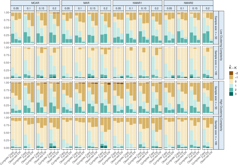
Figure 4: Accuracy of BIC, when used with each of the three methods, in recovering the true $K=3$, for different clustering complexities, sample sizes, missingness mechanisms and $\lambda\in\{0.05,0.1,0.15,0.2\}$. The display is in terms of the difference between $\hat{K}$ and $K$.

Figure 4 shows relatively good performance of “Observed EM” in estimating $K$, mildly underestimating $K$ for

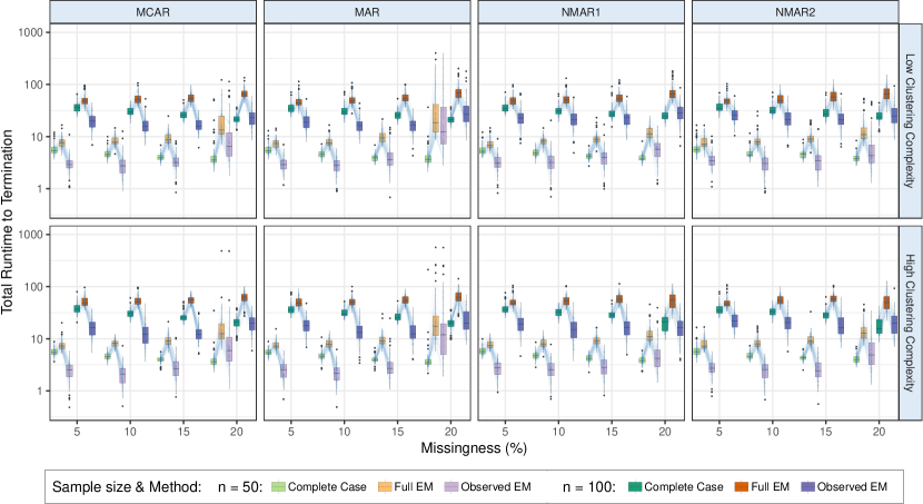
(a) Time to termination of the EM algorithms in each setting when estimating $K$ using BIC.

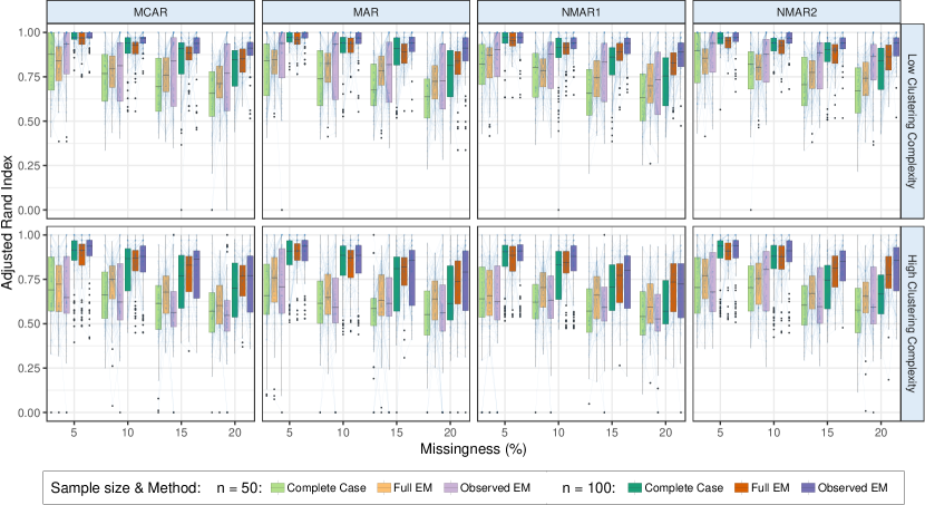
(b) Clustering performance of competing methods, as per ARI.

Figure 5: Comprehensive simulation results when $K$ is required to be estimated.

$n=50$, but not so much for the larger sample size. Performance for all methods worsens with higher clustering complexity, however “Complete Case” and “Full EM” moderately overestimate $K$ in all settings. As in the known true $K$ case, Figure 5a shows that “Observed EM” is substantially faster than “Full EM” and that, at least in the cases of low clustering complexity and with larger $n$, is the best overall performer (Figure 5b). With high clustering complexity, this trend is explicit with $n=100$ only for the NMAR2 case, and with lower proportions of missingness for the other three missingness mechanisms. For $n=50$ or with $n=100$ and MCAR, MAR, and NMAR1 missingness mechanisms under conditions of high clustering complexity, the performance of “Observed EM” relative to “Full EM” is more mixed with higher proportions of missingness.

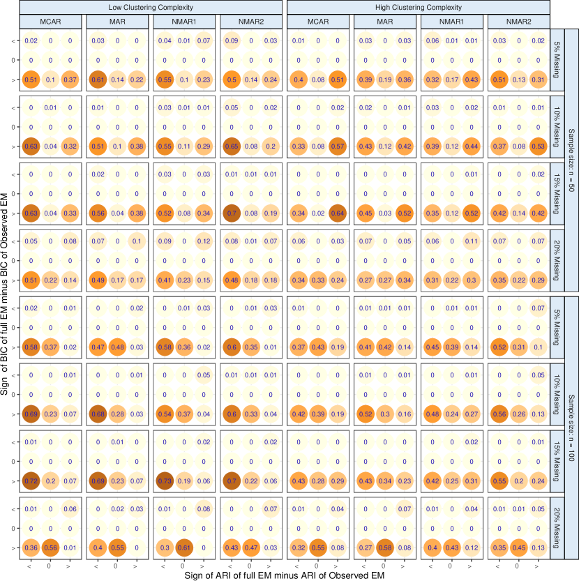
Figure 6: BIC relative to ARI for the two methods, for the different simulation settings. For each setting, we have cross-tabulated the relative frequency of datasets on which where the BIC of “Full EM” is less than (“$<$”), the same (“$0$”) or exceeds (“$>$”) that of “Observed EM” against the same for the ARI. Color intensity is proportional to the relative frequency.

Comment

A reviewer has asked us for insight into the reasons for the better performance of “Observed EM” over “Full EM” even when assumptions are far from MCAR. We surmise the reasons for this. Indeed, “Full EM” provides guaranteed local maxima of the EM (AECM) algorithm. Our modification does not, suffering, as it does, from possible premature termination. However, the objective log likelihood function, especially in the case of non-MCAR mechanisms, is not a completely accurate representation of the sampling mechanism that generated the data, and therefore, maximizing it may not be the golden bullet that solves the clustering problem. To evaluate if there indeed is evidence in support of this hypothesis, we compared the optimal BIC for “Full EM” and “Observed EM” and the ARI. (The BIC is a surrogate for the goodness of fit under the assumed loglikelihood model and the ARI is an indicator of cluster recovery and performance.) Figure 6 displays the results. We see that often “Full EM” is able to achieve a higher BIC than “Observed EM” but fails to get more credit for cluster recovery (per ARI) and this mismatch increases correspondingly with proportions of missingness in data. This phenomenon holds for both when the sample size is $n=50$ or $n=100$. Of course, this does not answer the question as to why “Observed EM” does better in terms of cluster recovery. Our hypothesis is that this happens because our CM-step updates for $\bm{\mu}_{k}$s and $\bm{\Sigma}_{k}$s use method-of-moments estimators and do not condition on the observed data. When the data are NMAR, the observed values are not directly informative of those that are missing because their values are related to their own missingness. We suspect that this aspect in our algorithm is what is allowing for better performance. Finally, finite mixture models provide only an indirect approach to clustering with parameter estimation and model selection happening first, followed by cluster assignment as a byproduct from the calculation of posterior probabilities of classification. Nevertheless, our performance evaluations establish “Observed EM” as a faster and competitive alternative to “Full EM”. We now apply it to the problem of characterizing gamma ray bursts.

IV Discovering the distinct kinds of Gamma Ray Bursts

Gamma-ray bursts (GRBs) are the brightest electromagnetic bursts known to occur in space and emanate from distant galaxies. Since their discovery, several causes of GRBs have been proposed [66, 67, 68, 69] and the existence of multiple sub-types [70, 71, 72, 73] hypothesized. To elucidate the origins of GRBs, it is of interest to determine the number and defining characteristics of these groups. Early work classified GRBs using one or two features, often using only burst duration [74]. It was argued that more variables were needed to fully account for the observed data structure [5, 75], leading to recent interest in clustering GRBs using more features. Subsequent analyses [19, 18, 76, 77] established five groups in the GRB dataset obtained from the most recent Burst and Transient Source Experiment (BATSE) 4Br catalog.

The BATSE 4Br catalog is the most comprehensive database of the duration, intensity, and composition of 1,973 GRBs, but the records are subject to missing values encoded as zeros [19, 18], leading to a total of 1,599 GRBs that are complete cases. There are up to nine features for each GRB, namely $T_{50}$, $T_{90}$, $F_{1}$, $F_{2}$, $F_{3}$, $F_{4}$, $P_{64}$, $P_{256}$, and $P_{1024}$, where $T_{\tau}$ denotes the time by which $\tau$% of the flux arrive, $P_{t}$ denotes the peak fluxes measured in bins of $t$ milliseconds, and $F_{s}$ represents the fluence in the $s$th spectral channel. Due to the extreme right-skewness in the distribution of these variables, we apply the customary base-10 logarithm transformation to all the variables, and for brevity, omit the logarithm in subsequent descriptions. ([76] however incorporated data-driven transformations in their analysis to address the skew.) The two duration variables $T_{50}$ and $T_{90}$ are observed for all 1973 GRBs. The three peak flux measurements are only missing in one GRB, while $F_{1}$, $F_{2}$, $F_{3}$ and $F_{4}$ are missing values in 29, 12, 6 and 339 GRBs [18]. Multivariate analysis of the GRBs has so far largely focused on the 1599 GRBs with complete records [19, 18, 76, 77, 5, 75]. On the other hand, [78] ignored the peak fluxes and the $F_{4}$ features and the 44 GRBs that were missing values for the other features and performed Gaussian mixture-model-based clustering for the 1929 GRBs and came up with three types of GRBs. They also tried to explain the results of [19] in the context of their findings. However, the analysis of  [18] on the complete dataset showed all nine variables to have clustering information. [18] also used the maximum marginal posterior probability to classify the remaining $n-n^{\prime}$ incomplete cases to the obtained cluster partition: however, this approach assumes that all the clusters are represented in the complete sample, an assumption that may be untenable, especially when the data are not MCAR. Therefore, it is of interest to include GRBs with partial records in our analysis and our development in this paper helps facilitate that investigation.

Since the imputation approaches performed poorly in our simulation assessments, we restricted our attention to the observed, full, and complete case EM style approaches, again with default settings. The “Observed EM” and “Full EM” methods preferred $\hat{K}=7$ clusters, as per BIC among candidates ranging from $K=1,\dots,10$, in contrast to previous reports of only two or three clusters obtained using a few features or the five clusters obtained using the complete dataset. Our methodology, applied on the 1599 complete GRB cases, also found five or six groups, though the latter was not conclusive, following [79], so we decide on five groups.  [18] also got five groups using the teigen software [49]. This is reassuring even though our method differs from that of teigen insofar as it allows for $\nu$, to vary across groups. We now discuss the results for the 7-groups solutions (and briefly, for the complete case 5-groups scenario).

Table Ib presents the estimated cluster proportions and degrees of freedom for the BIC-preferred K obtained using the three methods.

TABLE I: Estimated (a) mixing proportions $\hat{\pi}_{1},\ldots,\hat{\pi}_{\hat{K}}$ and (b) degrees of freedom $\hat{\nu}_{1},\ldots,\hat{\nu}_{\hat{K}}$, obtained after fitting the three approaches to the GRB dataset at the BIC-preferred $\hat{K}=5$ (for the complete case) and $\hat{K}=7$ for the other two cases.

Cluster	1	2	3	4	5	6	7
Complete Case	0.210	0.106	0.276	0.151	0.258	-	-
Full EM	0.191	0.086	0.246	0.083	0.187	0.081	0.126
Observed EM	0.204	0.079	0.215	0.096	0.214	0.079	0.113

(a) Estimated mixing proportions

1	2	3	4	5	6	7
24.9	9.8	11.8	12.2	39.3	-	-
24.2	9.8	14.8	161.6	200.0	9.2	26.9
29.7	9.8	14.7	42.1	79.0	7.8	71.3

(b) Estimated degrees of freedom

The three solutions disagree mildly in the estimated mixing proportions (but “Observed EM” tracks “Full EM” fairly well). The degrees of freedom are also different in a few cases. While the teigen solution in [18] found (all five $\nu$s to be 200), our “Complete Case” solution found much fatter-tailed $t$-mixture components. Figure 7 displays the estimated cluster means

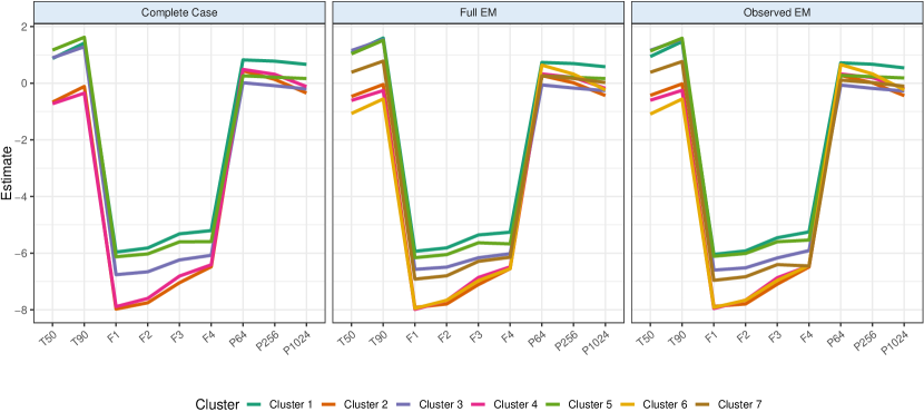
(a)

(b)

Figure 7: (a) Parallel coordinate plots of $\hat{\bm{\mu}}_{1},\ldots,\hat{\bm{\mu}}_{\hat{K}}$ and (b) heatmap of $\hat{\bm{\Sigma}}_{1},\ldots,\hat{\bm{\Sigma}}_{\hat{K}}$ for the BIC-selected $\hat{K}$ groups partition of the GRB data obtained using each of the three methods.

and scale parameters of the multivariate $t$-components. We note minor differences in the means and the scale parameters, with the “Observed EM” and “Full EM” cluster parameters being qualitatively the same. For the seven-groups solution, the “Full EM” had slightly higher log likelihood than the others, however, the main astrophysical properties of the solution is similar for both “Observed EM” and “Full EM” groups so we only discuss the “Observed EM” results.

[75] provided a novel approach to describing the properties of GRBs. This approach, also adopted by [19, 18, 76, 77], uses the average duration ($T_{90}$), total fluence ($F_{t}=F_{1}+F_{2}+F_{3}+F_{4}$), and spectral hardness ($H_{321}=F_{3}/(F_{1}+F_{2})$) to characterize the GRBs. (Note that these calculations use the GRB features in the original scale.) Using these values, we can classify the seven GRB “Observed EM” groups as long/bright/soft, short/faint/intermediate, long/faint/soft, short/faint/hard, long/intermediate/soft, very short/faint/hard, and short/intermediate/soft, in terms of their average duration/fluence/hardness. Further analysis of our results is outside the purview of this paper, but our groups are able to characterize GRBs more distinctly compared that in [19, 18, 76, 77] that used only the complete cases.

V Discussion

In this paper, we consider model-based clustering of partially recorded or otherwise incomplete data using all and only the observed values through the use of an observed data model. A corresponding approximate AECM algorithm for clustering of partially recorded data is developed and implemented in the R package MixtClust. When fitting finite mixtures of $t$ distributions to incomplete data for the purpose of clustering, integrating over the missing components has several benefits compared to complete case analysis or including the missing components in an EM algorithm: fewer computations are required in each EM iteration and the approach in our experiments appears to offer somewhat greater resistance to severe violations of the MCAR assumption. Based on the simulation experiments of Section III, we conclude that our approach is efficient and robust when compared to the corresponding complete case analysis and full EM based on finite mixture modeling with multivariate $t$ distributions. We also use our methodology to characterize GRBs in the BATSE 4Br catalog into seven sub-types with distinct and interpretable astrophysical properties.

Further consideration of the relative strengths and weaknesses between “Full EM” and our “Observed EM” approach is warranted. In particular, we need to get a better understanding for the reason why “Observed EM” performs better than “Full EM” with increasing deviations from MAR assumptions. The “Full EM” approach utilizes information on the observed values to inform the missing values, and we surmise that this information is beneficial for clustering performance when it is not (too) wrong, in contrast with the NMAR2 setting where “Observed EM” does better. However, as noted by the reviewer, we also believe that incorporating the missingness mechanism in the development of the modeling and the inference is a better approach and should be adopted: however, this is application-specific and requires knowledge of the specific mechanism causing the missingness. In the absence of information on missingness, we find that our approach does well, and is also faster, not only in terms of per iteration, but also in terms of the time to convergence. Further, our simulation experiments used the same number of initialization steps and convergence criteria for all methods, without regard to the fact that our “Observed EM” approach is by design faster than “Full EM”, so it would be interesting to compare performance with times set to be the same, and to see if we can recover the lost ground to “Full EM” using more initializations in the cases where we are currently out-performed. Also, while using the $t$ distribution for each cluster accommodates outliers, at least relative to a Gaussian distribution, it assumes that the clusters are ellipsoidally symmetric about their centers. Such an assumption may be unrealistic in practice, where clusters could be asymmetric. A natural extension of our work would incorporate skew-$t$ distributions for such cases or, alternatively, employ a symmetrizing transformation such as the Box-Cox transformation considered in finite mixture modeling by [80]. Several other lines of improvement are possible for our method. First, we only consider general covariance structure dispersion matrices, but in actuality a simpler structure may be adequate. Accordingly, future work can incorporate a family of eigen-decomposed covariance structures [35]. Second, we use a lack-of-progress criterion to assess convergence but it may be better to use alternative strategies such as Aitken’s acceleration [81] to compute an asymptotic estimate of the log likelihood as proposed by [82]. Finally, while we use BIC to select the optimal number of clusters, this does not account for the classification uncertainty in the fitted model as considered by the integrated completed likelihood (ICL) criterion of [83]. Thus, we see that while we have made some contributions to the goal of model-based clustering of partial records, a number of issues remain that merit further attention.

Data Availability

The GRB dataset used in this application is available at https://github.com/emilygoren/MixtClust.

Appendix A Derivations for the AECM steps

We provide here derivations for $\hat{\bm{\mu}}_{k}$ in (6) and $\hat{\bm{\Sigma}}_{k}$ in (8). From equation (84) of [84], we have

$$0\stackrel{{\scriptstyle\text{set}}}{{=}}\frac{\partial}{\partial\bm{\mu}_{k}}Q_{2}\left(\bm{\mu}_{k},\bm{\Sigma}_{k}\>|\>\hat{\bm{\Theta}}\right) =\frac{\partial}{\partial\bm{\mu}_{k}}\sum_{i=1}^{n}\frac{\hat{z}_{ik}}{2}\bigg{[}-\hat{w}_{ik}(\bm{y}_{i}-\bm{\mu}_{k})^{\prime}\bm{O}_{i}^{\prime}(\bm{O}_{i}\bm{\Sigma}_{k}\bm{O}_{i}^{\prime})^{-1}\bm{O}_{i}(\bm{y}_{i}-\bm{\mu}_{k})\bigg{]}$$

$$=\sum_{i=1}^{n}\hat{z}_{ik}\hat{w}_{ik}\bm{O}_{i}^{\prime}(\bm{O}_{i}\bm{\Sigma}_{k}\bm{O}_{i}^{\prime})^{-1}\bm{O}_{i}(\bm{y}_{i}-\bm{\mu}_{k}).\mbox{ This implies }$$

$$\sum_{i=1}^{n}\hat{z}_{ik}\hat{w}_{ik}\bm{O}_{i}^{\prime}(\bm{O}_{i}\bm{\Sigma}_{k}\bm{O}_{i}^{\prime})^{-1}\bm{O}_{i}\bm{y}_{i} =\sum_{i=1}^{n}\hat{z}_{ik}\hat{w}_{ik}\bm{O}_{i}^{\prime}(\bm{O}_{i}\bm{\Sigma}_{k}\bm{O}_{i}^{\prime})^{-1}\bm{O}_{i}\bm{\mu}_{k},$$

$$\quad\mbox{or}\quad\hat{\bm{\mu}}_{k} =\left[\left(\sum_{i=1}^{n}\hat{z}_{ik}\hat{w}_{ik}\bm{O}_{i}^{\prime}(\bm{O}_{i}\bm{\Sigma}_{k}\bm{O}_{i}^{\prime})^{-1}\bm{O}_{i}\right)\right]^{-1}\sum_{i=1}^{n}\hat{z}_{ik}\hat{w}_{ik}\bm{O}_{i}^{\prime}(\bm{O}_{i}\bm{\Sigma}_{k}\bm{O}_{i}^{\prime})^{-1}\bm{O}_{i}\bm{y}_{i}.$$

To reduce computational complexity, we may use the method-of-moments update for $\hat{\mu}$:

$$\hat{\mu}_{k}=\sum_{i=1}^{n}\frac{\hat{z}_{ik}}{2}\bigg{[}\bm{O}_{i}^{\prime}\bm{O}_{i}\bm{\Sigma}_{k}\bm{O}_{i}^{\prime}\bm{O}_{i}-\hat{w}_{ik}\bm{O}_{i}^{\prime}\bm{O}_{i}(\bm{y}_{i}-\hat{\bm{\mu}}_{k})(\bm{y}_{i}-\hat{\bm{\mu}}_{k})^{\prime}\bm{O}_{i}^{\prime}\bm{O}_{i}\bigg{]},$$

where $\sum_{i=1}^{n}\hat{z}_{ik}\hat{w}_{ik}\operatorname{diag}(\bm{a}_{i})$ is invertible if $\sum_{i=1}^{n}\hat{z}_{ik}\hat{w}_{ik}I(y_{ij}\text{ is observed})>0$ for $1\leq j\leq p$, and then check to ensure if the $Q_{1}$ function increases with this update, or revert back to the current value if it does not.

For the dispersion updates, we considering each pattern of missingness and use the selection matrices to expand to dimension $p\times p$,

$$0 \quad\stackrel{{\scriptstyle\text{set}}}{{=}}\frac{\partial}{\partial\bm{\Sigma}_{k}}Q_{2}\left(\hat{\bm{\mu}}_{k},\bm{\Sigma}_{k}\>|\>\hat{\bm{\Theta}}\right)$$

$$\quad=\frac{\partial}{\partial\bm{\Sigma}_{k}}\sum_{i=1}^{n}\frac{\hat{z}_{ik}}{2}\bigg{[}-\log\lvert\bm{O}_{i}\bm{\Sigma}_{k}\bm{O}_{i}^{\prime}\rvert-\hat{w}_{ik}(\bm{y}_{i}-\hat{\bm{\mu}}_{k})^{\prime}\bm{O}_{i}^{\prime}(\bm{O}_{i}\bm{\Sigma}_{k}\bm{O}_{i}^{\prime})^{-1}\bm{O}_{i}(\bm{y}_{i}-\hat{\bm{\mu}}_{k})\bigg{]}$$

$$\quad=\frac{\partial}{\partial\bm{\Sigma}_{k}}\sum_{i=1}^{n}\frac{\hat{z}_{ik}}{2}\bigg{[}\log\lvert(\bm{O}_{i}\bm{\Sigma}_{k}\bm{O}_{i}^{\prime})^{-1}\rvert-\hat{w}_{ik}\operatorname{tr}\left\{\bm{O}_{i}(\bm{y}_{i}-\hat{\bm{\mu}}_{k})(\bm{y}_{i}-\hat{\bm{\mu}}_{k})^{\prime}\bm{O}_{i}^{\prime}(\bm{O}_{i}\bm{\Sigma}_{k}\bm{O}_{i}^{\prime})^{-1}\right\}\bigg{]}$$

$$\quad=\sum_{i=1}^{n}\frac{\hat{z}_{ik}}{2}\bigg{[}\bm{O}_{i}^{\prime}\left(\bm{O}_{i}\bm{\Sigma}_{k}\bm{O}_{i}^{\prime}\right)^{-1}\bm{O}_{i}-\hat{w}_{ik}\bm{O}_{i}^{\prime}\left(\bm{O}_{i}\bm{\Sigma}_{k}\bm{O}_{i}^{\prime}\right)^{-1}\bm{O}_{i}(\bm{y}_{i}-\hat{\bm{\mu}}_{k})(\bm{y}_{i}-\hat{\bm{\mu}}_{k})^{\prime}\bm{O}_{i}^{\prime}\left(\bm{O}_{i}\bm{\Sigma}_{k}\bm{O}_{i}^{\prime}\right)^{-1}\bm{O}_{i}\bigg{]},$$

which does not provide a closed-form solution. We again propose a method-of-moments estimator for $\hat{\Sigma}_{k}$. Specifically, we propose the update

$$\hat{\bm{\Sigma}}_{k}=\left(\sum_{i=1}^{n}\hat{z}_{ik}\bm{a}_{i}\bm{a}_{i}^{\prime}\right)^{\odot-1}\odot\left(\sum_{i=1}^{n}\hat{z}_{ik}\hat{w}_{ik}\operatorname{diag}(\bm{a}_{i})(\bm{y}_{i}-\hat{\bm{\mu}}_{k})(\bm{y}_{i}-\hat{\bm{\mu}}_{k})^{\prime}\operatorname{diag}(\bm{a}_{i})\right),$$

and accept it if $Q_{2}$ increases, or revert back to the current solution.

Appendix B Initialization Effect on “Full EM”

The experiments of Section III-C2 demonstrated the good performance of “Observed EM” in terms of speed: the method was also shown to be competitive

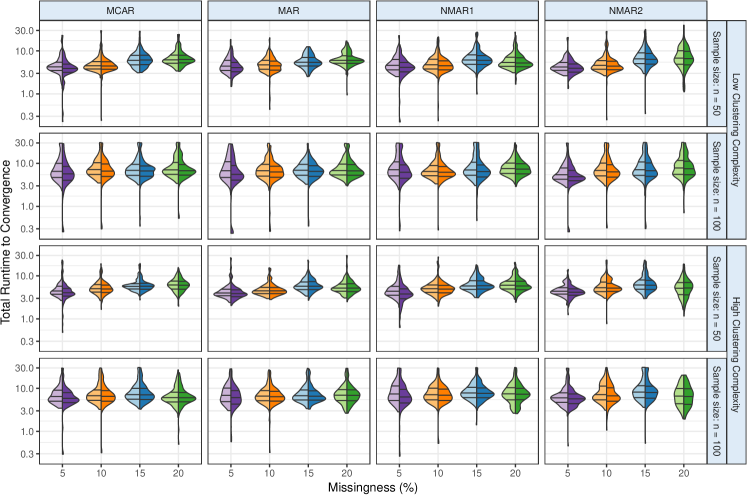
(a) Time to convergence of “Full EM” using Modified em-EM (left lobe of violin) and Rnd-EM (right lobe) methods.

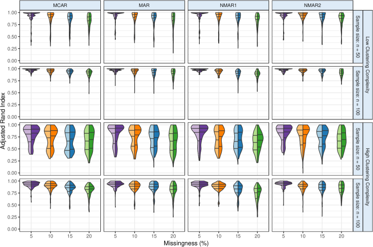
(b) Cluster recovery ability of “Full EM” using Modified em-EM (left lobe of violin) and Rnd-EM (right lobe) methods.

Figure 8: Evaluating the (a) speed and (b) performance of the “Full EM” algorithm using the Rnd-EM versus Modified em-EM initialization methods. Following [85], each split violin has the Modified em-EM on the left (lighter) lobe and the Rnd-EM on the right lobe. The bars denote the three quartiles of each violin.

in terms of clustering performance. Therefore, we performed another set of experiments, at the true $K=3$ that used “Full EM” with the Rnd-EM [55] and Modified em-EM [54] evaluations. Both methods used the same number of initializations ($K\sqrt{np}$) and ten long EM runs, but Modified em-EM also used ten “em” steps. Figure 8 displays the results through a split violin-plot [85] and indicates that there is not much difference in the distribution of either the time to convergence or in cluster recovery ability. We attribute the similar speed of Rnd-EM (with its zero “em” steps) and “Modified em-EM” to the fact that the former ends up often having more iterations in each of the long EM runs.

References

- [1] R. Maitra, “Clustering massive datasets with applications to software metrics and tomography,” Technometrics, vol. 43, no. 3, pp. 336–346, 2001.
- [2] D. M. Witten, “Classification and clustering of sequencing data using a poisson model,” The Annals of Applied Statistics, vol. 5, no. 4, pp. 2493–2518, 12 2011.
- [3] P. J. Turnbaugh, R. E. Ley, M. Hamady, C. M. Fraser-Liggett, R. Knight, and J. I. Gordon, “The human microbiome project,” Nature, vol. 449, no. 7164, p. 804, 2007.
- [4] J. Agarwal, R. Nagpal, and R. Sehgal, “Crime analysis using k-means clustering,” International Journal of Computer Applications, vol. 83, no. 4, 2013.
- [5] E. D. Feigelson and G. J. Babu, “Statistical Methodology for Large Astronomical Surveys,” in New Horizons from Multi-Wavelength Sky Surveys, ser. IAU Symposium, B. J. McLean, D. A. Golombek, J. J. E. Hayes, and H. E. Payne, Eds., vol. 179, 1998, p. 363.
- [6] J. MacQueen, “Some methods for classification and analysis of multivariate observations,” Proceedings of the Fifth Berkeley Symposium, vol. 1, pp. 281–297, 1967.
- [7] J. H. Ward, “Hierarchical grouping to optimize an objective function,” Journal of the American Statistical Association, vol. 58, pp. 236–244, 1963.
- [8] V. Melnykov and R. Maitra, “Finite mixture models and model-based clustering,” Statistics Surveys, vol. 4, pp. 80–116, 2010.
- [9] J. A. Hartigan and J. Hartigan, Clustering algorithms. New York: Wiley, 1975, vol. 209.
- [10] J. R. Kettenring, “The practice of cluster analysis,” Journal of classification, vol. 23, pp. 3–30, 2006.
- [11] R. Xu and D. C. Wunsch, Clustering. NJ, Hoboken: John Wiley & Sons, 2009.
- [12] P. D. McNicholas, Mixture model-based classification. Chapman and Hall/CRC, 2016.
- [13] C. Bouveyron, G. Celeux, B. T. Murphy, and A. E. Raftery, Model-Based Clustering and Classification for Data Science: With Applications in R. Cambridge Series in Statistical and Probabilistic Mathematics, 2019.
- [14] D. B. Rubin, “Inference and missing data,” Biometrika, vol. 63, no. 3, pp. 581–592, 1976.
- [15] R. J. Little and D. B. Rubin, Statistical analysis with missing data. John Wiley & Sons, 2014, vol. 1.
- [16] K. L. Wagstaff and V. G. Laidler, “Making the most of missing values: Object clustering with partial data in astronomy,” in Astronomical Data Analysis Software and Systems XIV, vol. 347, 2005, p. 172.
- [17] R. J. Hathaway and J. C. Bezdek, “Fuzzy c-means clustering of incomplete data,” IEEE Transactions on Systems, Man, and Cybernetics, Part B (Cybernetics), vol. 31, no. 5, pp. 735–744, Oct 2001.
- [18] S. Chattopadhyay and R. Maitra, “Multivariate -mixture-model-based cluster analysis of BATSE catalogue establishes importance of all observed parameters, confirms five distinct ellipsoidal sub-populations of gamma-ray bursts,” Monthly Notices of the Royal Astronomical Society, vol. 481, no. 3, pp. 3196–3209, 07 2018.
- [19] ——, “Gaussian-mixture-model-based cluster analysis finds five kinds of gamma-ray bursts in the BATSE catalogue,” Monthly Notices of the Royal Astronomical Society, vol. 469, no. 3, pp. 3374–3389, 2017.
- [20] S. Buuren and K. Groothuis-Oudshoorn, “mice: Multivariate imputation by chained equations in R,” Journal of statistical software, vol. 45, no. 3, 2011.
- [21] A. R. T. Donders, G. J. van der Heijden, T. Stijnen, and K. G. Moons, “Review: a gentle introduction to imputation of missing values,” Journal of clinical epidemiology, vol. 59, no. 10, pp. 1087–1091, 2006.
- [22] J. Honaker, G. King, and M. Blackwell, “Amelia ii: A program for missing data,” Journal of statistical software, vol. 45, no. 7, pp. 1–47, 2011.
- [23] L. A. F. Park, J. C. Bezdek, C. Leckie, R. Kotagiri, J. Bailey, and M. Palaniswami, “Visual assessment of clustering tendency for incomplete data,” IEEE Transactions on Knowledge and Data Engineering, vol. 28, no. 12, pp. 3409–3422, Dec 2016.
- [24] J. K. Dixon, “Pattern recognition with partly missing data,” IEEE Transactions on Systems, Man, and Cybernetics, vol. 9, no. 10, pp. 617–621, Oct 1979.
- [25] Q. Zhang and Z. Chen, “A distributed weighted possibilistic c-means algorithm for clustering incomplete big sensor data,” International Journal of Distributed Sensor Networks, vol. 10, no. 5, p. 430814, 2014.
- [26] M. Sarkar and T.-Y. Leong, “Fuzzy -means clustering with missing values,” in Proceedings of American Medical Informatics Association Annual Symposium (AMIA), 2001, pp. 588–592.
- [27] K. Simiński, “Clustering with missing values,” Fundamenta informaticae, vol. 123, no. 3, pp. 331–350, 2013.
- [28] ——, “Rough fuzzy subspace clustering for data with missing values.” Computing & Informatics, vol. 33, no. 1, 2014.
- [29] ——, “Rough subspace neuro-fuzzy system,” Fuzzy Sets and Systems, vol. 269, pp. 30–46, 2015.
- [30] K. Wagstaff, “Clustering with missing values: No imputation required,” in Classification, Clustering, and Data Mining Applications, D. Banks, L. House, F. McMorris, P. Arabie, and W. Gaul, Eds. Springer, 2004, pp. 649–658.
- [31] J. T. Chi, E. C. Chi, and R. G. Baraniuk, “k-pod: A method for k-means clustering of missing data,” The American Statistician, vol. 70, no. 1, pp. 91–99, 2016.
- [32] K. Lange, MM Optimization Algorithms. SIAM, 2016.
- [33] A. Lithio and R. Maitra, “An efficient k-means-type algorithm for clustering datasets with incomplete records,” Statistical Analysis and Data Mining: The ASA Data Science Journal, vol. 11, no. 6, pp. 296–311, 2018.
- [34] J. A. Hartigan and M. A. Wong, “A -means clustering algorithm,” Applied Statistics, vol. 28, pp. 100–108, 1979.
- [35] J. D. Banfield and A. E. Raftery, “Model-based Gaussian and non-Gaussian clustering,” Biometrics, vol. 49, pp. 803–821, 1993.
- [36] G. Celeux and G. Govaert, “Gaussian parsimonious clustering models,” Computational Statistics and Data Analysis, vol. 28, pp. 781–93, 1995.
- [37] G. McLachlan and D. Peel, Robust cluster analysis via mixtures of multivariate t distributions. Berlin, Heidelberg: Springer Berlin Heidelberg, 1998, pp. 658–666.
- [38] D. Peel and G. McLachlan, “Robust mixture modeling using the t distribution,” Statistics and Computing, vol. 10, p. 339:348, 2000.
- [39] B. Lindsay, Mixture models: theory, geometry and applications, 1995.
- [40] P. C. Mahalanobis, “On the generalized distance in statistics.” National Institute of Science of India, 1936.
- [41] H. Wang, Q. Zhang, B. Luo, and S. Wei, “Robust mixture modeling using multivariate t distribution with missing information,” Pattern Recogn. Lett., vol. 25, pp. 701–710, April 2004.
- [42] A. P. Dempster, N. M. Laird, and D. B. Rubin, “Maximum likelihood for incomplete data via the EM algorithm (with discussion),” Jounal of the Royal Statistical Society, Series B, vol. 39, pp. 1–38, 1977.
- [43] T.-I. Lin, “Learning from incomplete data via parameterized t mixture models through eigenvalue decomposition,” Computational Statistics & Data Analysis, vol. 71, pp. 183 – 195, 2014.
- [44] W.-L. Wang and T.-I. Lin, “Robust model-based clustering via mixtures of skew-t distributions with missing information,” Advances in Data Analysis and Classification, vol. 9, no. 4, pp. 423–445, 2015, cited By 3.
- [45] Y. Wei, Y. Tang, and P. D. McNicholas, “Mixtures of generalized hyperbolic distributions and mixtures of skew-t distributions for model-based clustering with incomplete data,” Computational Statistics & Data Analysis, vol. 130, pp. 18–41, 2019.
- [46] X. Meng and D. van Dyk, “The EM algorithm — an old folk-song sung to a fast new tune (with discussion),” Journal of the Royal Statistical Society B, vol. 59, pp. 511–567, 1997.
- [47] T.-I. Lin, H. J. Ho, and P. S. Shen, “Computationally efficient learning of multivariate t mixture models with missing information,” Computational Statistics, vol. 24, no. 3, pp. 375–392, Aug 2009.
- [48] E. A. Cornish, “The multivariate t-distribution associated with a set of normal sample deviates,” Australian Journal of Physics, vol. 7, pp. 531–542, 1954.
- [49] J. L. Andrews, J. R. Wickins, N. M. Boers, and P. D. McNicholas, “teigen: An R package for model-based clustering and classification via the multivariate t distribution,” Journal of Statistical Software, vol. 83, no. 1, pp. 1–32, 2018.
- [50] J. L. Andrews and P. D. McNicholas, “Model-based clustering, classification, and discriminant analysis via mixtures of multivariate t-distributions,” Statistics and Computing, vol. 22, no. 5, pp. 1021–1029, Sep 2012.
- [51] R. P. Brent, “An algorithm with guaranteed convergence for finding a zero of a function,” The Computer Journal, vol. 14, no. 4, pp. 422–425, 1971.
- [52] G. McLachlan and T. Krishnan, The EM Algorithm and Extensions, 2nd ed. New York: Wiley, 2008.
- [53] C. Biernacki, G. Celeux, and G. Govaert, “Choosing starting values for the EM algorithm for getting the highest likelihood in multivariate Gaussian mixture models,” Computational Statistics and Data Analysis, vol. 413, pp. 561–575, 2003.
- [54] R. Maitra, “On the expectation-maximization algorithm for Rice-Rayleigh mixtures with application to estimating the noise parameter in magnitude MR datasets,” Sankhyā: The Indian Journal of Statistics, Series B, vol. 75, no. 2, p. 293–318, 2013.
- [55] ——, “Initializing partition-optimization algorithms,” IEEE/ACM Transactions on Computational Biology and Bioinformatics, vol. 6, pp. 144–157, 2009.
- [56] G. Schwarz, “Estimating the dimensions of a model,” Annals of Statistics, vol. 6, pp. 461–464, 1978.
- [57] J. L. Andrews, P. D. McNicholas, and S. Subedi, “Model-based classification via mixtures of multivariate t distributions,” Computational Statistics and Data Analysis, vol. 55, no. 1, pp. 520 – 529, 2011.
- [58] C. Fraley and A. E. Raftery, “MCLUST version 3 for R: Normal mixture modeling and model-based clustering,” University of Washington, Department of Statistics, Seattle, WA, Tech. Rep. 504, 2006.
- [59] R. Maitra and V. Melnykov, “Simulating data to study performance of finite mixture modeling and clustering algorithms,” Journal of Computational and Graphical Statistics, vol. 19, no. 2, pp. 354–376, 2010.
- [60] V. Melnykov, W.-C. Chen, and R. Maitra, “MixSim: An R package for simulating data to study performance of clustering algorithms,” Journal of Statistical Software, vol. 51, no. 12, pp. 1–25, 2012.
- [61] V. Melnykov and R. Maitra, “CARP: Software for fishing out good clustering algorithms,” Journal of Machine Learning Research, vol. 12, pp. 69 – 73, 2011.
- [62] R. Maitra, “A re-defined and generalized percent-overlap-of-activation measure for studies of fMRI reproducibility and its use in identifying outlier activation maps,” Neuroimage, vol. 50, no. 1, pp. 124–135, 2010.
- [63] Y.-S. Su, A. Gelman, J. Hill, and M. Yajima, “Multiple imputation with diagnostics (mi) in R: Opening windows into the black box,” Journal of Statistical Software, vol. 45, no. 2, pp. 1–31, 2011.
- [64] L. Hubert and P. Arabie, “Comparing partitions,” Journal of classification, vol. 2, no. 1, pp. 193–218, 1985.
- [65] W. M. Rand, “Objective criteria for the evaluation of clustering methods,” Journal of the American Statistical Association, vol. 66, pp. 846–850, 1971.
- [66] T. Chattopadhyay, R. Misra, A. K. Chattopadhyay, and M. Naskar, “Statistical evidence for three classes of gamma-ray bursts,” The Astrophysical Journal, vol. 667, no. 2, p. 1017, 2007.
- [67] T. Piran, “The physics of gamma-ray bursts,” Rev. Mod. Phys., vol. 76, pp. 1143–1210, Jan 2005.
- [68] M. Ackermann, M. Ajello, K. Asano, W. Atwood, M. Axelsson, L. Baldini, J. Ballet, G. Barbiellini, M. Baring, D. Bastieri et al., “Fermi-lat observations of the gamma-ray burst grb 130427a,” Science, vol. 343, no. 6166, pp. 42–47, 2014.
- [69] B. Gendre, G. Stratta, J. Atteia, S. Basa, M. Boër, D. Coward, S. Cutini, V. D’Elia, E. Howell, A. Klotz, and L. Piro, “The ultra-long gamma-ray burst 111209a: the collapse of a blue supergiant?” The Astrophysical Journal, vol. 766, no. 1, p. 30, 2013.
- [70] A. Shahmoradi and R. J. Nemiroff, “Short versus long gamma-ray bursts: a comprehensive study of energetics and prompt gamma-ray correlations,” Monthly Notices of the Royal Astronomical Society, vol. 451, pp. 126–143, Jul. 2015.
- [71] E. P. Mazets, S. V. Golenetskii, V. N. Ilinskii, V. N. Panov, R. L. Aptekar, I. A. Gurian, M. P. Proskura, I. A. Sokolov, Z. I. Sokolova, and T. V. Kharitonova, “Catalog of cosmic gamma-ray bursts from the KONUS experiment data. I.” Astrophysics and Space Science, vol. 80, pp. 3–83, Nov. 1981.
- [72] J. P. Norris, T. L. Cline, U. D. Desai, and B. J. Teegarden, “Frequency of fast, narrow gamma-ray bursts,” Nature, vol. 308, p. 434, Mar. 1984.
- [73] J.-P. Dezalay, C. Barat, R. Talon, R. Syunyaev, O. Terekhov, and A. Kuznetsov, “Short cosmic events - A subset of classical GRBs?” in American Institute of Physics Conference Series, ser. American Institute of Physics Conference Series, W. S. Paciesas and G. J. Fishman, Eds., vol. 265, 1992, pp. 304–309.
- [74] C. Kouveliotou, C. A. Meegan, G. J. Fishman, N. P. Bhat, M. S. Briggs, T. M. Koshut, W. S. Paciesas, and G. N. Pendleton, “Identification of two classes of gamma-ray bursts,” The Astrophysical Journal, vol. 413, pp. L101–L104, 1993.
- [75] S. Mukherjee, E. D. Feigelson, G. Jogesh Babu, F. Murtagh, C. Fraley, and A. Raftery, “Three Types of Gamma-Ray Bursts,” The Astrophysical Journal, vol. 508, pp. 314–327, Nov. 1998.
- [76] N. Berry and R. Maitra, “TiK-means: Transformation-infused -means clustering for skewed groups,” Statistical Analysis and Data Mining – The ASA Data Science Journal, vol. 12, no. 3, pp. 223–233, 2019.
- [77] I. A. Almodóvar-Rivera and R. Maitra, “Kernel-estimated nonparametric overlap-based syncytial clustering,” Journal of Machine Learning Research, vol. 21, no. 122, pp. 1–54, 2020.
- [78] B. G. Tóth, I. I. Rácz, and I. Horváth, “Gaussian-mixture-model-based cluster analysis of gamma-ray bursts in the BATSE catalog,” Monthly Notices of the Royal Astronomical Society, vol. 486, no. 4, pp. 4823–4828, 05 2019. [Online]. Available: https://doi.org/10.1093/mnras/stz1188
- [79] R. E. Kass and A. E. Raftery, “Bayes factors,” Journal of the American Statistical Association, vol. 90, pp. 773–795, 1995.
- [80] K. Lo and R. Gottardo, “Flexible mixture modeling via the multivariate t-distribution with the Box-Cox transformation: an alternative to the skew t-distribution,” Statistics and Computing, vol. 2, no. 1, pp. 33–52, 2012.
- [81] A. Aitken, “A series formula for the roots of algebraic and transcendental equations,” Proceedings of the Royal Society of Edinburgh, vol. 45, no. 1, pp. 14–22, 1926.
- [82] D. Böhning, E. Dietz, R. Schaub, P. Schlattmann, and B. Lindsay, “The distribution of the likelihood ratio for mixtures of densities from the one-parameter exponential family,” Annals of the Institute of Statistical Mathematics, vol. 46(2), pp. 373–388, 1994.
- [83] C. Biernacki, G. Celeux, and E. M. Gold, “Assessing a mixture model for clustering with the integrated completed likelihood,” IEEE Transactions on Pattern Analysis and Machine Intelligence, vol. 22, pp. 719–725, 2000.
- [84] K. B. Petersen and M. S. Pedersen, “The matrix cookbook,” 2012. [Online]. Available: http://matrixcookbook.com
- [85] R. Maitra, “Efficient bandwidth estimation in 2D filtered backprojection reconstruction,” IEEE Transactions on Image Processing, vol. 28, no. 11, pp. 5610–5619, 2019.