Planet-induced radio emission from the coronae of M dwarfs: the case of Prox Cen and AU Mic

Abstract

There have recently been detections of radio emission from low-mass stars, some of which are indicative of star-planet interactions. Motivated by these exciting new results, in this paper we present Alfvén wave-driven stellar wind models of the two active planet-hosting M dwarfs Prox Cen and AU Mic. Our models incorporate large-scale photospheric magnetic field maps reconstructed using the Zeeman-Doppler Imaging method. We obtain a mass-loss rate of $0.25~{}\dot{M}_{\sun}$ for the wind of Prox Cen. For the young dwarf AU Mic, we explore two cases: a low and high mass-loss rate. Depending on the properties of the Alfvén waves which heat the corona in our wind models, we obtain mass-loss rates of $27$ and $590~{}\dot{M}_{\sun}$ for AU Mic. We use our stellar wind models to assess the generation of electron cyclotron maser instability emission in both systems, through a mechanism analogous to the sub-Alfvénic Jupiter-Io interaction. For Prox Cen we do not find any feasible scenario where the planet can induce radio emission in the star’s corona, as the planet orbits too far from the star in the super-Alfvénic regime. However, in the case that AU Mic has a stellar wind mass-loss rate of $27~{}\dot{M}_{\sun}$, we find that both planets b and c in the system can induce radio emission from $\sim 10$ MHz – 3 GHz in the corona of the host star for the majority of their orbits, with peak flux densities of $\sim 10$ mJy. Detection of such radio emission would allow us to place an upper limit on the mass-loss rate of the star.

1 Introduction

Many theoretical works have aimed to identify potential targets for the detection of exoplanetary radio emission (Grießmeier et al., 2007; Vidotto et al., 2015; Vidotto & Donati, 2017; Kavanagh et al., 2019). A model that is commonly used to estimate the generation of radio emission from exoplanets is the radiometric Bode’s law, which extrapolates the observed relation between the radio power emitted from the magnetised solar system objects and the incident solar wind power (Zarka, 2007). In this model, the interaction between the planet’s magnetosphere and the magnetised stellar wind of its host star leads to reconnection in the planet’s magnetotail. This reconnection then accelerates electrons towards the planet’s poles, creating emission through the electron cyclotron maser instability (ECMI).

In these works, hot Jupiters have often been selected as suitable candidates for radio detection. As they are exposed to harsh stellar wind conditions due to their proximity to their host stars (Vidotto et al., 2015), they are expected to produce much higher radio powers than those observed in the solar system (Zarka et al., 2001). This emission can only be generated if hot Jupiters are magnetised. Given that the emission mechanism is ECMI, it occurs at the cyclotron frequency $\nu=2.8~{}B$ MHz, where $B$ is the magnetic field strength in gauss (G). Zaghoo & Collins (2018) estimated that hot Jupiters could harbour magnetic fields with strengths of 1 – 10 G. In this range, these field strengths would correspond to radio emission from 2.8 – 28 MHz.

Despite hot Jupiters being seemingly favourable sources of detectable low frequency radio emission, many radio surveys of these systems have found little evidence of such emission (Smith et al., 2009; Lazio et al., 2010; Lecavelier des Etangs et al., 2013; de Gasperin et al., 2020; Narang et al., 2021). Numerous explanations have been proposed for the lack of detections, such as a mismatch between the emitted and observation frequency (Bastian et al., 2000), the emission being beamed out of our line of sight (Smith et al., 2009), and absorption of the emission by the stellar wind of the host star (Vidotto & Donati, 2017; Kavanagh et al., 2019; Kavanagh & Vidotto, 2020). Intriguingly, Turner et al. (2021) recently detected radio emission at $\sim 30$ MHz from the hot Jupiter host $\tau$ Boo. They suggest that this emission could be indicative of ECMI generated in the orbiting planet’s magnetic field. Follow-up observations will be required however in order to investigate this further.

An alternative unipolar model for the generation of radio emission via ECMI in exoplanetary systems has also been proposed, analogous to the sub-Alfvénic interaction between Jupiter and its moon Io (Neubauer, 1980; Zarka, 1998; Saur et al., 2004; Zarka, 2007; Grießmeier et al., 2007). In this model, the host star and planet take the roles of Jupiter and Io respectively. If the planet orbits with a sub-Alfvénic velocity relative to the wind of its host star, it can generate Alfvén waves that travel back towards the star (Ip et al., 2004; McIvor et al., 2006; Lanza, 2012; Turnpenney et al., 2018; Strugarek et al., 2019; Vedantham et al., 2020). A fraction of the wave energy produced in this interaction is expected to dissipate and produce radio emission via ECMI in the corona of the host star (Turnpenney et al., 2018).

Due to the increasing sensitivity of radio telescopes such as LOFAR, M dwarfs are beginning to light up the radio sky at low frequencies (Callingham et al., submitted). One such system is the quiescent M dwarf GJ 1151, which was recently detected to be a source of 120 – 160 MHz emission by Vedantham et al. (2020). The authors illustrated that the observed emission is consistent with ECMI from the star induced by an Earth-sized planet orbiting in the sub-Alfvénic regime with a period of 1 – 5 days. Prior to this detection, there had been no evidence to suggest GJ 1151 is host to a planet. There has been some discussion in the literature recently about the existence of such a planet. Mahadevan et al. (2021) have suggested that a planet orbits the star in a 2-day orbit, whereas Perger et al. (2021) have ruled this out, placing a mass upper limit of 1.2 Earth on a planet in a 5-day orbit. Follow-up observations of the system will be needed to further assess if the radio emission is of a planet-induced origin.

M dwarfs typically exhibit strong magnetic fields, with maximum large-scale strengths ranging from $\sim 100$ G – 1 kG (Donati et al., 2008; Morin et al., 2010; Shulyak et al., 2019). If an M dwarf is host to a planet that orbits in the sub-Alfvénic regime, the planet could induce radio emission from the star’s corona via ECMI at frequencies up to 280 MHz – 2.8 GHz. Planet-induced emission from M dwarfs therefore could be distinguished from emission predicted with the radiometric Bode’s law, due to the different frequency ranges.

The M dwarf Proxima Centauri (Prox Cen) is our closest stellar neighbour, which also hosts a planet that is expected to be Earth-sized (Anglada-Escudé et al., 2016). Naturally, being so close to us we want to understand both the habitability of the orbiting planet and the system’s potential for producing planet-induced radio emission. An important step in answering this question is to assess the stellar wind environment around the planet. Prox Cen is expected to have a relatively weak stellar wind, with a mass-loss rate of $\dot{M}<0.2~{}\dot{M}_{\sun}$ (Wood et al., 2001), where $\dot{M}_{\sun}=2\times 10^{-14}~{}M_{\sun}~{}\textrm{yr}^{-1}$ is the solar wind mass-loss rate. The star also possesses a strong large-scale surface magnetic field of $\sim 200$ G (Klein et al., 2021). Its proximity to Earth along with its potentially habitable planet make it an interesting system to search for planet-induced radio emission.

AU Microscopii (AU Mic) is a young M dwarf which also shows potential for detecting planet-induced radio emission. It lies just under 10 pc away from Earth, and has recently been discovered to host two Neptune-sized close-in planets (Plavchan et al., 2020; Martioli et al., 2020a). We list the properties of the AU Mic system along with those for Prox Cen in Table 1. While planets b and c orbiting AU Mic are not likely to be habitable, their proximity to the host star makes them ideal candidates for inducing radio emission in the corona of the host star. The stellar wind mass-loss rate of AU Mic is relatively unconstrained. Models of interactions between the stellar wind and debris disk in the system estimate a mass-loss rate from 10 $\dot{M}_{\sun}$ (Plavchan et al., 2009) up to 1000 $\dot{M}_{\sun}$ (Chiang & Fung, 2017). Its large-scale surface magnetic field is also quite strong, with a strength of $\sim 500$ G (Klein et al., 2020). The two close-in planets along with the star’s strong magnetic field make it a very suitable candidate for planet-induced radio emission.

In this paper, we use the magnetic field maps reconstructed by Klein et al. (2021) and Klein et al. (2020) to model the stellar winds of the two M dwarfs Prox Cen and AU Mic respectively. We use our 3D Alfvén wave-driven stellar wind models to investigate if the orbiting planets can induce the generation of ECMI emission in the coronae of their host stars. We then illustrate how the detection of planet-induced radio emission can be used to constrain properties of the wind of the host star.

Table 1: Stellar and planetary parameters for the Prox Cen and AU Mic systems.

Parameter	Prox Cen	Reference	AU Mic		Reference
Stellar mass ($M_{\star}$)	0.12 $M_{\sun}$	1	0.50 $M_{\sun}$		2
Stellar radius ($R_{\star}$)	0.14 $R_{\sun}$	1	0.75 $R_{\sun}$		2
Stellar wind mass-loss rate ($\dot{M}$)	< 0.2 $\dot{M}_{\sun}$	3	$10~{}\dot{M}_{\sun}$, $1000~{}\dot{M}_{\sun}$		4, 5
Average surface stellar magnetic field strength	200 G	6	500 G		7
Spectral type	M5.5V	1	M1V		8
Stellar rotation period	83 days	1	4.86 days		2
Distance ($d$)	1.30 pc	1	9.79 pc		2
	Planet b		Planet b	Planet c
Planetary mass ($M_{\textrm{p}}$)	> 1.27 $M_{\textrm{\earth}}$	1	1.00 $M_{\textrm{Nep}}$	1.7 – 27.7 $M_{\textrm{\earth}}$	9
Planetary radius ($R_{\textrm{p}}$)	-	-	1.13 $R_{\textrm{Nep}}$	0.91 $R_{\textrm{Nep}}$	9
Planetary orbital distance ($a$)	74.0 $R_{\star}$	1	18.5 $R_{\star}$	26.9 $R_{\star}$	9
Planetary orbital period	11.2 days	1	8.46 days	18.9 days	9
1: Anglada-Escudé et al. (2016); 2: Plavchan et al. (2020); 3: Wood et al. (2001); 4: Plavchan et al. (2009); 5: Chiang & Fung (2017); 6: Klein et al. (2021); 7; Klein et al. (2020); 8: Martioli et al. (2020b); 9: Martioli et al. (2020a)

2 Modelling the winds of M-dwarfs

To model the stellar winds of Prox Cen and AU Mic we use the Alfvén wave solar model (AWSoM, van der Holst et al., 2014) implemented in the 3D magnetohydrodynamic (MHD) code BATS-R-US (Powell et al., 1999), which is part of the Space Weather Modelling Framework (Tóth et al., 2012). In the AWSoM model, Alfvén waves are injected at the base of the chromosphere where they propagate, reflect, and dissipate. The dissipation of the Alfvén waves heats the corona, which in turn drives the stellar wind outflow. The AWSoM model has been validated against observations of the solar corona (van der Holst et al., 2014; Jin et al., 2017), and has also been applied to study the stellar wind environments of other systems (see Garraffo et al., 2017; Boro Saikia et al., 2020; Alvarado-Gómez et al., 2020; Ó Fionnagáin et al., 2021).

In our models, we set boundary conditions for the radial magnetic field, Alfvén wave flux, plasma density and temperature at the base of the chromosphere. For the magnetic field we use maximum-entropy maps reconstructed from spectropolarimetric observations for the two stars by Klein et al. (2021) and Klein et al. (2020) via the Zeeman-Doppler Imaging method (Donati & Landstreet, 2009). These are shown in Figure 1. The input for the Alfvén wave flux in our model is given in units of flux per unit magnetic field strength $S_{\textrm{A}}/B$. We refer to this as the ‘Alfvén wave flux-to-magnetic field ratio’, for which we adopt a variety of values (see Section 3). We fix the density and temperature at the base of the chromosphere as $2\times 10^{10}$ cm^-3 and $5\times 10^{4}$ K respectively in our models, the same as chosen by Alvarado-Gómez et al. (2020). These values are also typically used for the Sun (see Sokolov et al., 2013).

The corona is heated through a turbulent energy cascade in our model, which is produced by the reflection and dissipation of Alfvén waves in the local plasma environment. The wave dissipation rate depends on the transverse correlation length $L_{\perp}$, which in turn is proportional to $B^{-1/2}$ (Hollweg, 1986). In our model the transverse correlation length is given in terms of the proportionality constant $L_{\perp}\sqrt{B}$. We adopt the default value of $L_{\perp}\sqrt{B}=1.5\times 10^{9}$ cm $\sqrt{\textrm{G}}$ for this (van der Holst et al., 2014). We also include both collisional and collisionless heat conduction, radiative cooling, and stochastic heating in our models, as described in van der Holst et al. (2014). We fix the adiabatic index to be $5/3$.

Our computational grid is spherical and extends from the base of the chromosphere to 100 times the stellar radius $R_{\star}$. The maximum resolution in our grid is $\sim 5\times 10^{-4}$ $R_{\star}$. We also adaptively-resolve current sheet regions in our grid. The number of cells in our grid is $\sim 6$ million. We iteratively solve the MHD equations until the model reaches a steady state. We take this to be when the mass-loss rate, open magnetic flux, and angular momentum-loss rate of the wind vary by less than 10 percent between iterations.

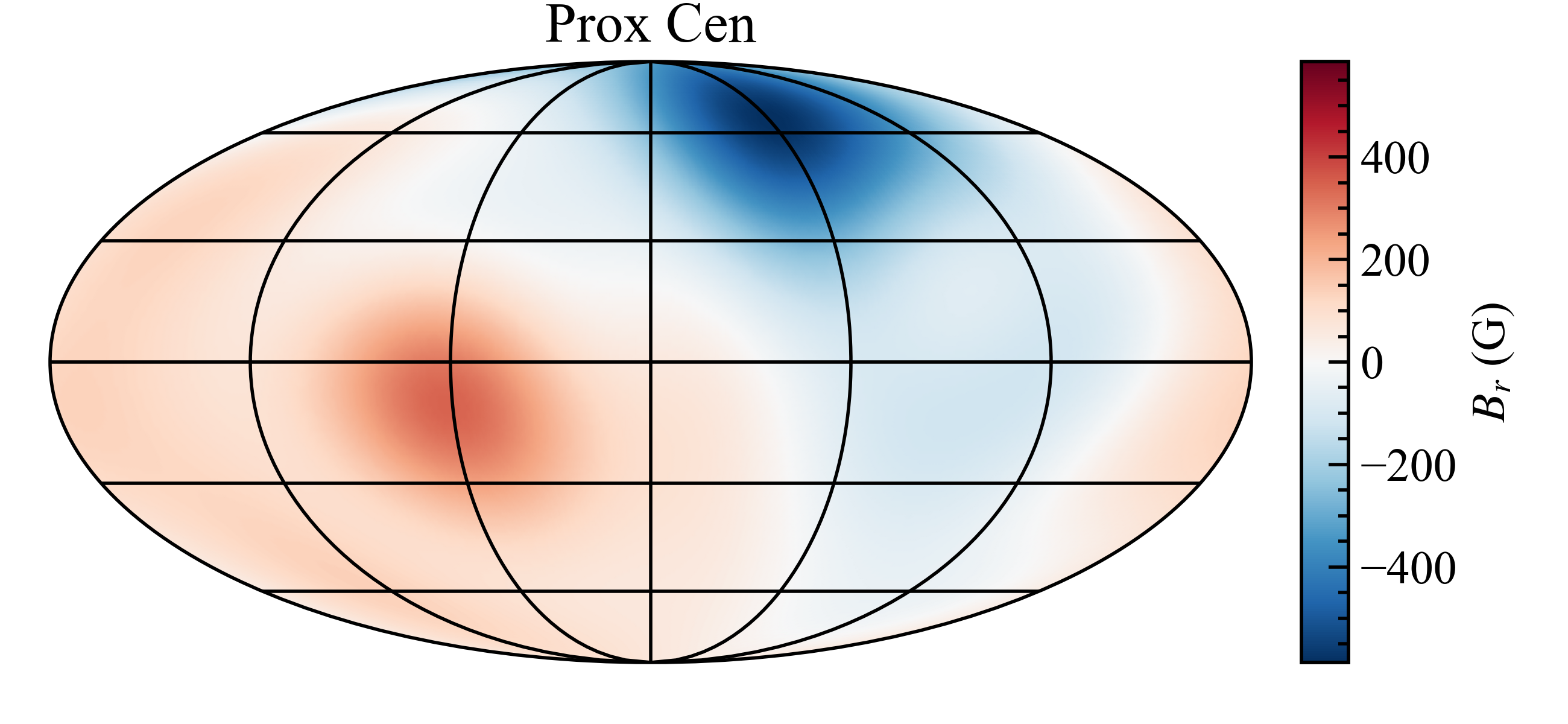
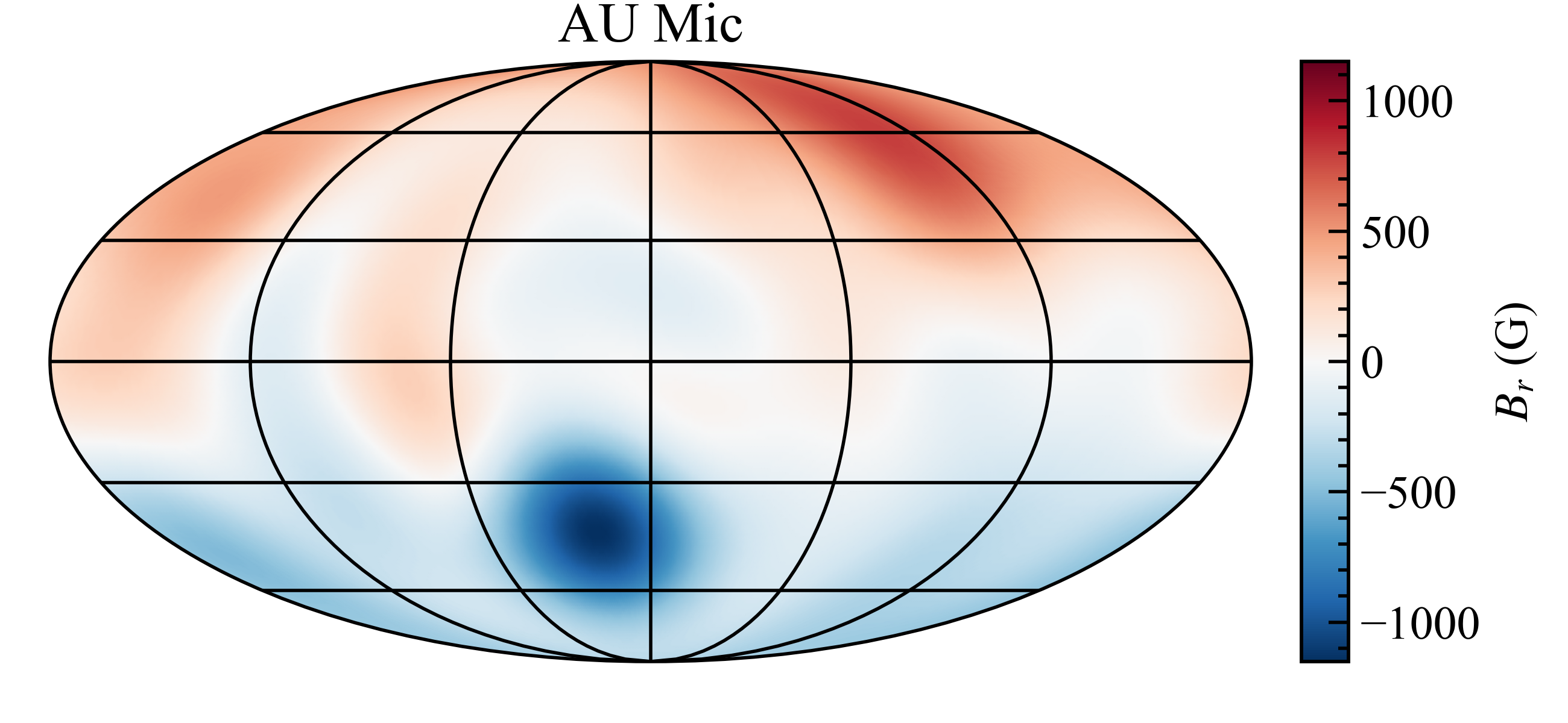
Figure 1: Radial photospheric magnetic field of Prox Cen (top) and AU Mic (bottom), reconstructed by Klein et al. (2021) and Klein et al. (2020) respectively. We implement these maps at the inner boundary of our stellar wind simulations for the two stars.

3 Stellar wind environments of the M-dwarfs

3.1 Prox Cen

Using an Alfvén wave flux-to-magnetic field ratio of $S_{\textrm{A}}/B=5\times 10^{4}$ erg s^-1 cm^-2 G^-1, we obtain a stellar wind with a mass-loss rate of $\dot{M}=0.25~{}\dot{M}_{\sun}$ for Prox Cen. This is in agreement with the upper limit obtained by Wood et al. (2001). The rest of the free parameters in the model are as described in Section 2. Our calculated mass-loss rate is in line with other published works on the wind of Prox Cen, which used proxies for the surface magnetic field (Garraffo et al., 2016; Alvarado-Gómez et al., 2020).

Figure 2 shows a 3D view of the simulated wind for Prox Cen. We see that the planet orbits in a super-Alfvénic regime for the entirety of its orbit. Therefore, we do not expect any unipolar planet-induced radio emission from Prox Cen during the epoch of the observations from which the magnetic field map was reconstructed (April - July 2017, Klein et al., 2021). Note that we assume that the orbital plane of the planet is perpendicular to the rotation axis of the star.

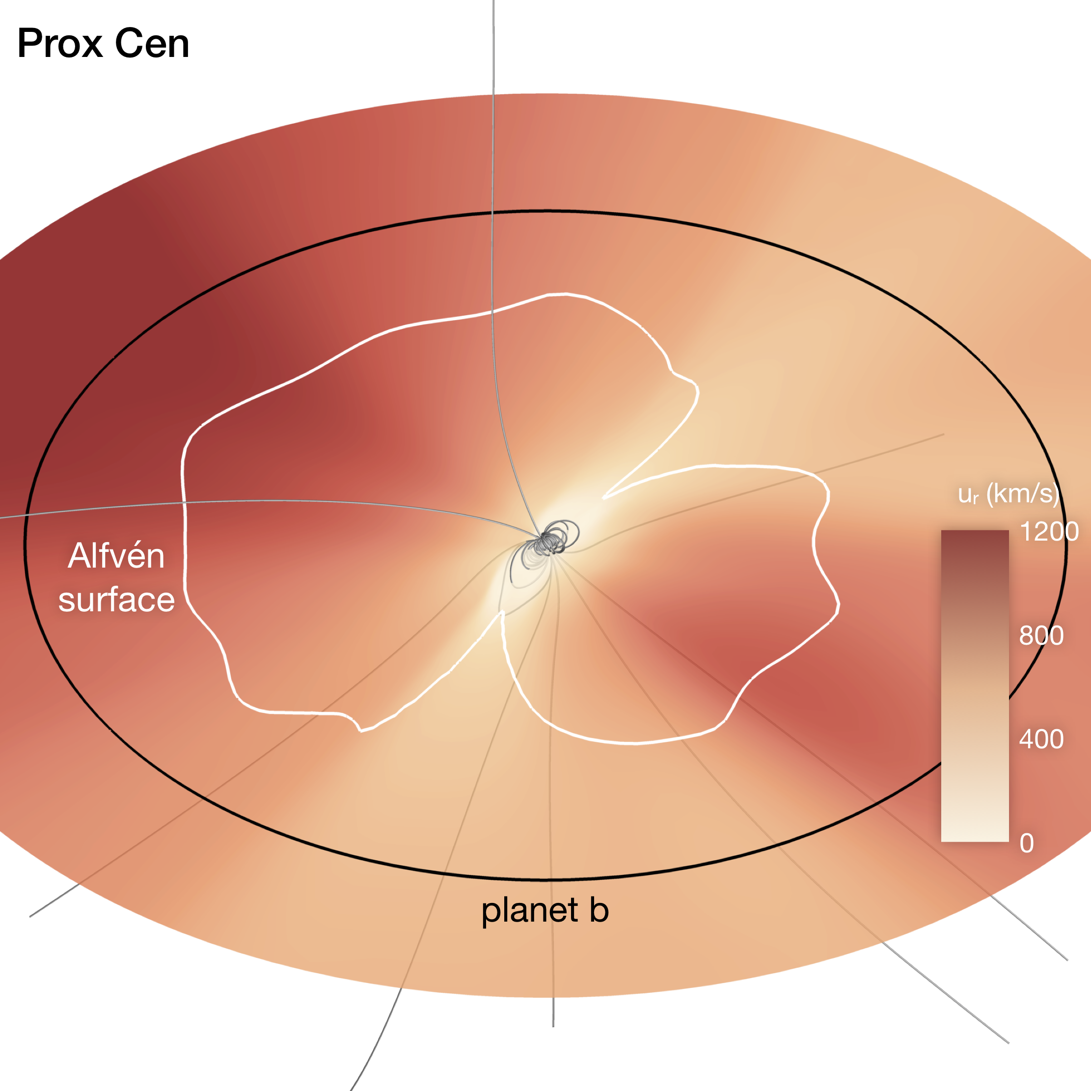
Figure 2: Simulated stellar wind of Prox Cen. The grey lines illustrate the large-scale magnetic field of the star which is embedded in the wind. The orbit of Prox Cen b is shown as a black circle, and the white line corresponds to where the Alfvén Mach number $M_{\textrm{A}}=1$ (see Equation 1). The contour in the orbital plane is coloured by the wind radial velocity ($u_{r}$).

3.2 AU Mic

To investigate the two estimated mass-loss rates for AU Mic, we use two different values for the Alfvén wave flux-to-magnetic field ratio. Again, the values used for the rest of the free parameters in the model are given in Section 2. For a value of $S_{\textrm{A}}/B=1.1\times 10^{5}$ erg s^-1 cm^-2 G^-1 (Sokolov et al., 2013), we obtain a stellar wind mass-loss rate of $27~{}\dot{M}_{\sun}$ for AU Mic. We refer to this as the ‘Low $\dot{M}$’ model for the star. Increasing the Alfvén wave flux-to-magnetic field ratio to $S_{\textrm{A}}/B=6\times 10^{6}$ erg s^-1 cm^-2 G^-1, we find that the mass-loss rate increases to a value of $590~{}\dot{M}_{\sun}$. We refer to this as the ‘High $\dot{M}$’ model. Figure 3 shows a 3D view of both stellar wind models for AU Mic. We take both planets to orbit perpendicular to the stellar rotation axis, as both planets transit the star with orbital inclinations of $\sim 90^{\circ}$ (Martioli et al., 2020a), with the orbit of planet b being aligned with the rotation axis of the star (Martioli et al., 2020b).

In the case of the Low $\dot{M}$ model (left panel of Figure 3), we find that both planets b and c orbit in the sub-Alfvénic regime for the majority of their orbit. This means that the two planets could induce the generation of radio emission along the lines connecting the planet to the star (Turnpenney et al., 2018; Vedantham et al., 2020). For the High $\dot{M}$ model however, both planets are in the super-Alfvénic regime for their entire orbit (right panel of Figure 3), as the wind is much denser than the Low $\dot{M}$ model. As a result, we do not expect planet-induced radio emission from AU Mic in the case that it has a high mass-loss rate.

We now estimate the maximum mass-loss rate for AU Mic at which the planets can induce radio emission. Using a least-squares method, we fit our data with a power law between the mass-loss rate and maximum size of the Alfvén surface in the orbital plane $R_{\textrm{A, orb}}^{\textrm{max}}$. For our data, we obtain a fit of $\dot{M}=9.6\times 10^{5}(R_{\textrm{A, orb}}^{\textrm{max}})^{-2.6}~{}\dot{M}_{\odot}$, where $R_{\textrm{A, orb}}^{\textrm{max}}$ is in stellar radii. For both planets to be in sub-Alfvénic orbits at least partially, the maximum size of the Alfvén surface must be greater than the orbital distance of planet c. Substituting this orbital distance of $26.9~{}R_{\star}$ into our power law fit to our data, we find that AU Mic would need to have a mass-loss rate of $\lesssim 190~{}\dot{M}_{\odot}$ in order for planet-induced radio emission to be generated in its corona. Detection of such emission would therefore allow us to place an upper limit of $\lesssim 190~{}\dot{M}_{\sun}$ on the mass-loss rate of AU Mic. Note that in either case, radio emission could still be generated from the planet’s own magnetosphere (see Vidotto & Donati, 2017; Kavanagh et al., 2019; Kavanagh & Vidotto, 2020). We explore the scenario for the generation of planet-induced radio emission in AU Mic’s corona further in Section 4.1.

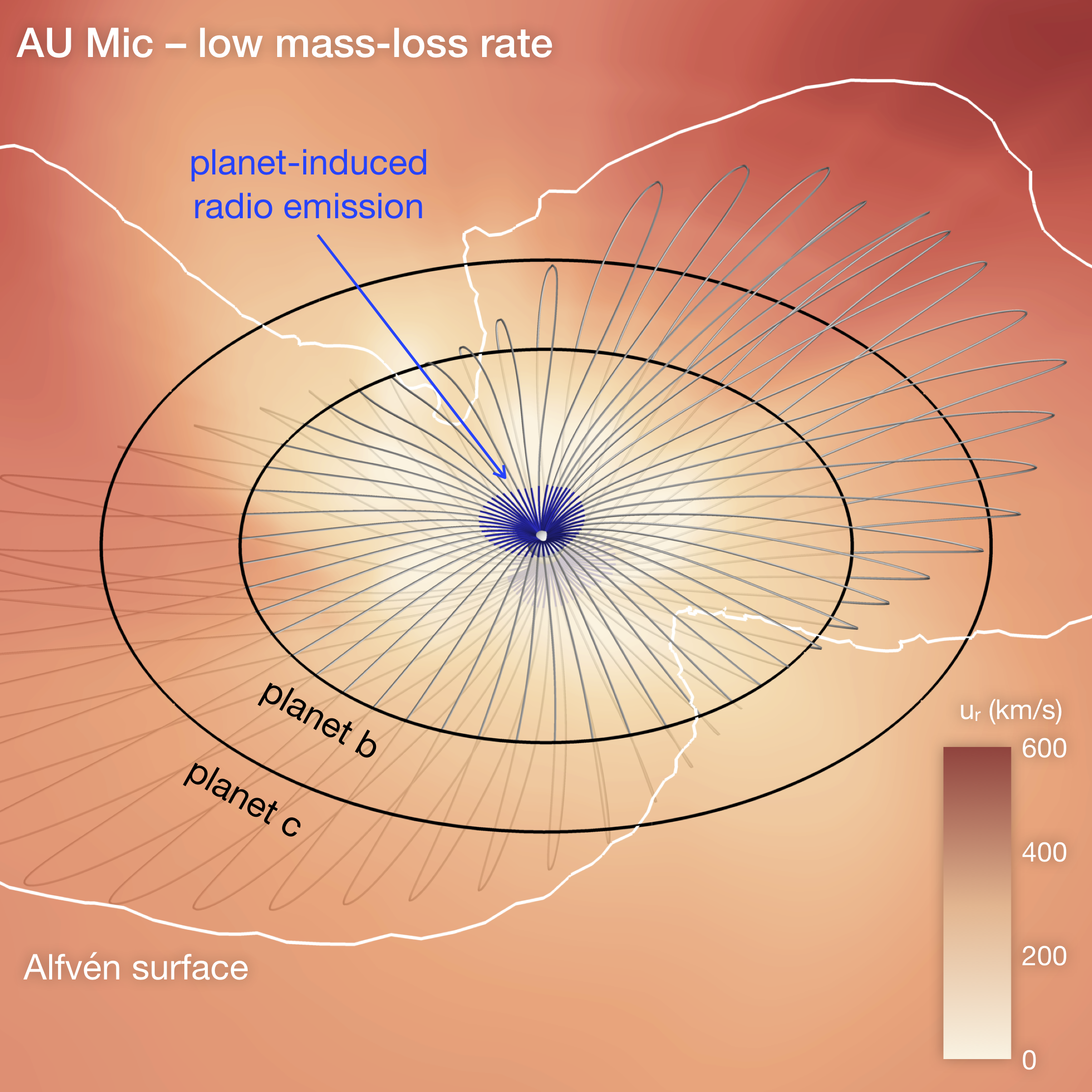
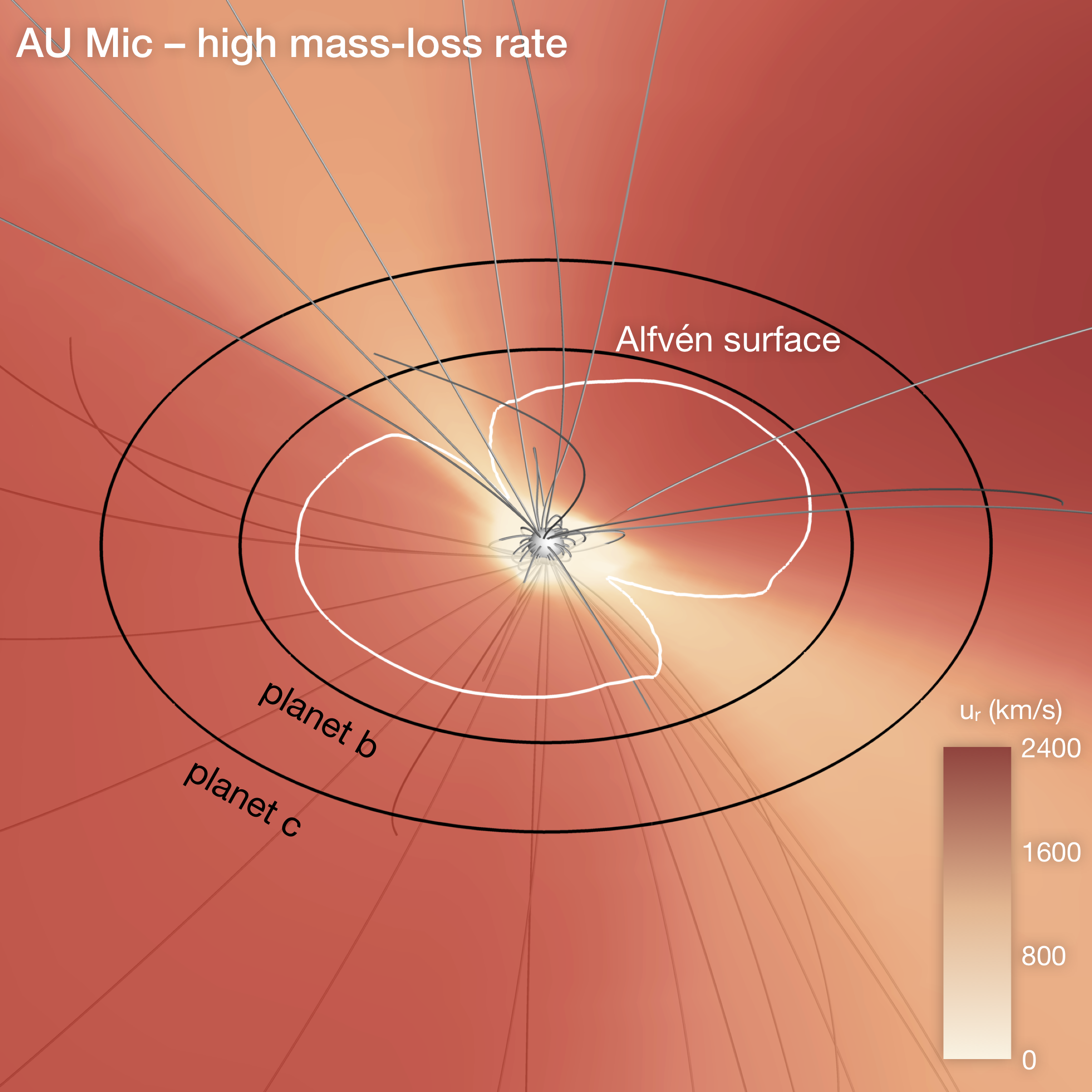
Figure 3: Left: Low $\dot{M}$ model of the stellar wind of AU Mic. The orbits of planets b and c are shown as black circles, and the white line corresponds to where the Alfvén Mach number $M_{\textrm{A}}=1$ (see Equation 1). The contour in the orbital plane is coloured by the wind radial velocity ($u_{r}$). The grey lines show the stellar magnetic field lines that connect to the orbit of planet b. Each of these lines is a closed loop, and connects back to the star in both the Northern and Southern hemisphere. The blue shaded region of each line illustrates where planet b can induce the generation of radio emission via ECMI (see Equation 6). Note that planet c can also induce generation, but for clarity we omit these field lines. Right: High $\dot{M}$ model for AU Mic. Both planets b and c orbit in the super-Alfvénic regime in this scenario. Note that the magnetic field lines shown here do not connect to the orbit of either planet.

4 Planet-induced radio emission

4.1 AU Mic

Here, we describe our model we use to estimate the radio emission induced in the corona of AU Mic by planets b and c, in the scenario where the star has a mass-loss rate of $\lesssim 190~{}\dot{M}_{\sun}$. We use our Low $\dot{M}$ model data in our calculations. A planet is said to be in the sub-Alfvénic regime when the Alfvén Mach number is less than 1:

$$M_{\textrm{A}}=\frac{\Delta u}{u_{\textrm{A}}}<1.$$ (1)

Here, $\Delta u$ is the relative velocity between the stellar wind velocity $u$ and planet orbital velocity $u_{\textrm{p}}$:

$$\boldsymbol{\Delta u}=\boldsymbol{u}-\boldsymbol{u_{\textrm{p}}}.$$ (2)

The orbital velocity of the planet is $\boldsymbol{u_{\textrm{p}}}=\sqrt{GM_{\star}/a}~{}\boldsymbol{\hat{\phi}}$, where $G$ is the gravitational constant, $M_{\star}$ is the stellar mass, $a$ is the orbital distance, and $\boldsymbol{\hat{\phi}}$ is the azimuthal angle. In equation 1, $u_{\textrm{A}}$ is the Alfvén velocity of the stellar wind at the planet:

$$u_{\textrm{A}}=\frac{B}{\sqrt{4\pi\rho}},$$ (3)

where $B$ and $\rho$ are the stellar wind magnetic field strength and density respectively.

The power of the Alfvén waves produced by a planet orbiting in the sub-Alfvénic regime is (Saur et al., 2013):

$$P=\pi^{1/2}R^{2}B\rho^{1/2}\Delta u^{2}\sin^{2}\theta,$$ (4)

where $R$ is the radius of the obstacle, and $\theta$ is the angle between the vectors $\boldsymbol{B}$ and $\boldsymbol{\Delta u}$. Assuming the planet is unmagnetised, we use the planetary radius $R_{\textrm{p}}$ for the obstacle radius. The waves travel towards the star along the magnetic field line connecting it to the planet, and a fraction of their energy is converted into ECMI emission. The emission occurs at the local cyclotron frequency (Turnpenney et al., 2018):

$$\nu=2.8\times 10^{-3}\frac{B}{\textrm{1 G}}~{}\textrm{GHz}.$$ (5)

We assume emission can be generated everywhere along the magnetic field line connecting the planet to the star, provided the cyclotron frequency exceeds the plasma frequency:

$$\nu>\nu_{\textrm{p}}=9\times 10^{-6}\sqrt{\frac{n_{\textrm{e}}}{\textrm{1 cm}^{-3}}}~{}\textrm{GHz}.$$ (6)

Here $n_{\textrm{e}}$ is the electron number density.

We trace each magnetic field line that connects to the planet’s orbit back to the point where it connects to the surface of AU Mic. Both planets orbit through closed-field regions of the star’s large-scale magnetic field, which predominantly resembles an aligned dipole (Klein et al., 2021). This means that ECMI emission can be generated in both the Northern and Southern hemisphere of AU Mic. Checking the condition in Equation 6 is satisfied, we extract the magnetic field strength along the line and compute the cyclotron frequency with Equation 5. These regions are highlighted in blue in the left panel of Figure 3. We then compute the flux density observed at a distance $d$ from the system as

$$F_{\nu}=\frac{\varepsilon P}{\Omega d^{2}\nu}.$$ (7)

Here $\varepsilon$ is the fraction of the wave energy from the interaction which is converted into ECMI emission. Observations of the Jupiter-Io interaction indicate that $\varepsilon\approx 0.01$ (Turnpenney et al., 2018), which we adopt here. $\Omega$ is the solid angle of the emission beam. Again, we adopt the observed value for the Jupiter-Io interaction of $\Omega=1.6$ sr (Zarka et al., 2004).

We show the flux density induced by planet b in the Northern and Southern hemispheres of AU Mic as a function of its orbital phase in Figure 4. The flux density is colour-coded with the frequency of the emission. We find that planet b can induce emission from $\sim 10$ MHz – 3 GHz in both hemispheres, with flux densities ranging from $\sim 10^{-2}$ – 10 mJy. Higher flux densities correspond to lower frequencies (see Equation 7). Note that planet c also can induce radio emission in this frequency range, albeit with flux densities that are around an order of magnitude lower. This is due to the term $B\rho^{1/2}$ in Equation 4 dominating at larger orbital distances, as the density and magnetic field strength drop off radially. As the planets orbit with different rotation periods however, they may produce distinct radio signals at different frequencies and periodicities that could be detected.

In Figure 4 we also highlight the emission that is generated at 140 MHz, which corresponds to the middle of the frequency range of 120 – 160 MHz at which some M dwarfs have recently been detected (Vedantham et al., 2020, Callingham et al., submitted). Vedantham et al. (2020) suggested that their observations of emission from the M dwarf GJ 1151 may be generated by a planet orbiting in the sub-Alfvénic regime. At 140 MHz, our results bear a strong resemblance to the observations of GJ 1151: both have flux densities of about 1 mJy which exhibit temporal variations. It would be very useful to obtain radio and near-simultaneous spectropolarimetric observations of M dwarfs similar to these systems so that this scenario could be explored further.

Time-varying nonthermal radio emission from AU Mic at 1.5 GHz was reported by Cox & Gibson (1985), with flux densities ranging from 2 – 3 mJy. Compared to our predicted fluxes induced by planet b at this frequency range, the observed flux densities are about an order of magnitude larger. If this emission was induced by either planet, it would require a much higher radio power than we predict. This could occur if the wind properties were enhanced in response to an increase in the magnetic field strength of AU Mic. Alternatively, if the radius of the obstacle were $R\approx 3.2~{}R_{\textrm{p}}$, the radio power estimated using Equation 4 would increase by an order of magnitude. We estimate that this would be the size of the magnetopause of planet b if it had a dipolar field strength of $\sim 6$ G (see Vidotto & Donati, 2017; Kavanagh et al., 2019). Therefore, not only could detection of planet-induced radio emission allow us to constrain the mass-loss rate of the host star, but also the magnetic field strength of the planet itself, if it is magnetised. As there is no polarisation information reported by Cox & Gibson (1985) however, we unfortunately cannot assess the origin of this emission this further. Future observations with the VLA, MWA, or upcoming SKA radio telescope would certainly be beneficial to search for radio signals in the frequency range at which we predict AU Mic could emit planet-induced radio emission. A derivable quantity such as the brightness temperature of the emission could allow for detected polarised emission indicative of being planet-induced to be distinguished from flaring emission, as has been illustrated by Vedantham et al. (2020).

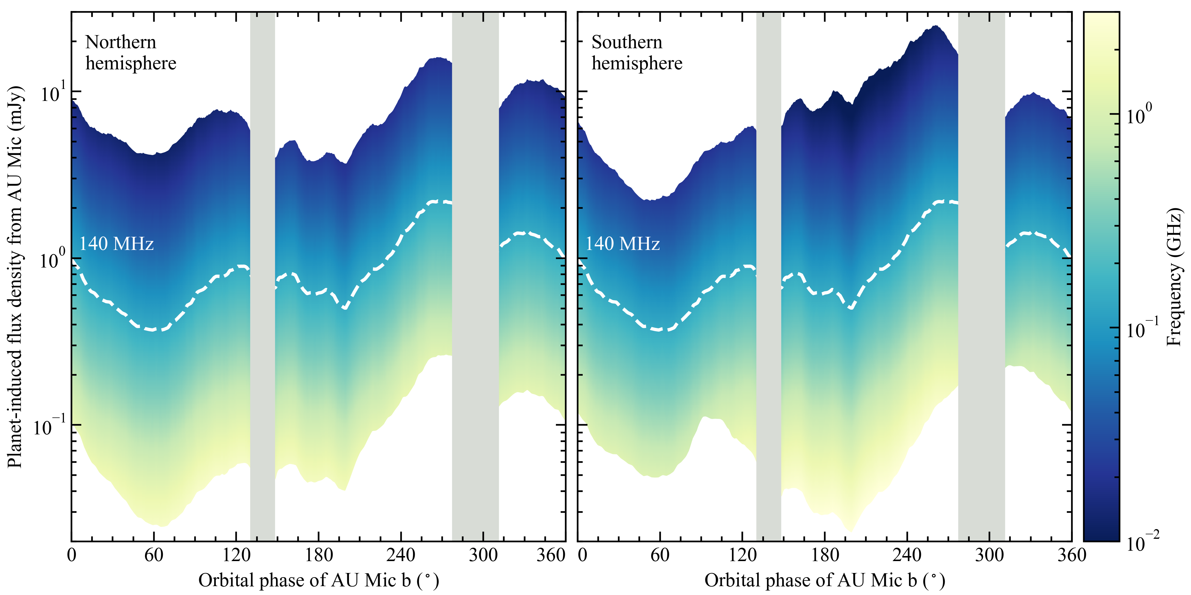
Figure 4: Radio spectrum of AU Mic induced by planet b in the Northern and Southern hemispheres of the star’s corona (left and right panels respectively). Emission generated at 140 MHz is highlighted with a white dashed line. This is the middle frequency of the observing band at which radio emission was recently detected from the M dwarf GJ 1151 by Vedantham et al. (2020), which is suspected of being induced by an orbiting planet. The grey shaded areas illustrate the region where the orbit of planet is in the super-Alfvénic regime. No emission can generate in these regions (see Equation 6).

4.2 Prox Cen

Radio emission from 1.1 – 3.1 GHz was recently detected from Prox Cen by Pérez-Torres et al. (2020). These observations occurred during April 2017, at same epoch the spectropolarimetric observations began for Prox Cen (Klein et al., 2021). Pérez-Torres et al. (2020) suggested that this emission could be indicative of star-planet interactions. If this is the case, it would require the planet to be orbiting in the sub-Alfvénic regime. Our wind model of Prox Cen however, which has a mass-loss rate in agreement with the upper limit obtained by Wood et al. (2001), shows that planet b orbits in the super-Alfvénic regime for the entirety of its orbit. In order for the planet to induce radio emission from the corona of Prox Cen, the Alfvén surface would need to extend beyond the planet’s orbit. This would require the mass-loss rate of the star to be significantly lower than the value we obtained of $0.25~{}\dot{M}_{\sun}$.

To investigate this further, we ran two additional stellar wind models for Prox Cen, with Alfvén wave flux-to-magnetic field ratios of $S_{\textrm{A}}/B=1.1\times 10^{4}$ erg s^-1 cm^-2 G^-1 and $1.1\times 10^{5}$ erg s^-1 cm^-2 G^-1. We obtain mass-loss rates of $0.05~{}\dot{M}_{\sun}$ and $0.57~{}\dot{M}_{\sun}$ respectively for these two simulations. In the case of the lower mass-loss rate model, we find that the planet still orbits entirely in a super-Alfvénic regime. Naturally, this is also the case for the model $0.57~{}\dot{M}_{\sun}$, which has a denser wind than our model presented in Section 3.1.

We now use these results, combined with those from Section 3.1, to estimate the Alfvén wave flux-to-magnetic field ratio and mass-loss rate needed to place Prox Cen b in a sub-Alfvénic orbit. We first perform a least-squares power law fit between the Alfvén wave flux-to-magnetic field ratio $S_{\textrm{A}}/B$ and mass-loss rate $\dot{M}$, and find that $\dot{M}=2.6\times 10^{-6}(S_{\textrm{A}}/B)^{1.06}~{}\dot{M}_{\sun}$ for Prox Cen, where $S_{\textrm{A}}/B$ is in erg s^-1 cm^-2 G^-1. The effects of changing $S_{\textrm{A}}/B$ on the solar wind mass-loss rate were investigated by Boro Saikia et al. (2020) using the AWSoM model. For comparison, we fit the same power law to their results, and find that during solar minimum $\dot{M}\propto(S_{\textrm{A}}/B)^{1.37}$, and during solar maximum $\dot{M}\propto(S_{\textrm{A}}/B)^{1.42}$ (using the $l_{\textrm{max}}=5$ data in their Tables F.1 and F.2).

For Prox Cen, we compute the maximum radius of the Alfvén surface $R_{\textrm{A, orb}}^{\textrm{max}}$ in the orbital plane of the planet for each plot, and plot it with its corresponding Alfvén wave flux-to-magnetic field ratio and mass-loss rate in Figure 5. Again, performing a least-squares power law fit between $R_{\textrm{A, orb}}^{\textrm{max}}$ and $S_{\textrm{A}}/B$, we estimate that an Alfvén wave flux-to-magnetic field ratio of $<5.3\times 10^{3}$ erg s^-1 cm^-2 G^-1 is required in order to place the plane in a sub-Alfvénic orbit. This corresponds to a stellar wind mass-loss rate of $<2.3\times 10^{-2}~{}\dot{M}_{\sun}$, which is an order of magnitude lower than the upper limit obtained by Wood et al. (2001).

Figure 5: Average radius of the Alfvén surface in the orbital plane of Prox Cen b vs. the Alfvén wave flux-to-magnetic field ratio (red diamonds). The upper $x$-axis is scaled accordingly based on the mass-loss rate of each wind simulation. The red dashed line illustrates our least-squares power law fit to the datapoints. We extrapolate this fit to estimate the Alfvén wave flux-to-magnetic field ratio required for the Alfvén surface to exceed the orbital distance of the planet (blue horizontal line). If this condition is satisfied, the planet can induce the generation of radio emission in the corona of the Prox Cen. This region is shown in grey on the left-hand side. We find that an Alfvén wave flux-to-magnetic field ratio of $\leq 2.7\times 10^{-3}$ erg s^-1 cm^-2 G^-1 is needed for the planet to orbit inside the Alfvén surface. This corresponds to mass-loss rate of $\leq 1.1\times 10^{-2}~{}\dot{M}_{\sun}$ for Prox Cen.

5 Discussion

There are some caveats to our planet-induced radio emission model. Firstly, we assume that the emission is always visible to the observer. However, it is well-established from observations of the Jupiter-Io interaction that the emission generated in this interaction is beamed in a hollow cone (see Zarka et al., 2004). As a result, if the emission can be generated it would likely be beamed in and out of the line of sight towards the system. Therefore, our results represent the best-case scenario where we always see the emission. We also do not account for the relative rotational motion between the star and planet, which would effect which stellar magnetic field line connects to the planet at any given time. Doing so would allow for us to estimate the temporal variations one would see observing the system, if this emission were detectable.

We also note that the higher radio fluxes we estimate for AU Mic in the case of a low mass-loss rate correspond to lower frequencies. However, as was shown by Kavanagh & Vidotto (2020), low frequency radio emission could suffer from significant attenuation from the stellar wind. We computed the thermal spectrum of AU Mic’s low mass-loss rate wind using the model developed by Ó Fionnagáin et al. (2019a, b), and found that the wind is optically thick below $\sim 0.1$ GHz. This means that a significant amount of the low frequency planet-induced emission ($<0.1$ GHz) we predict could be absorbed by the stellar wind. Note that we compute a peak flux density of $\sim 0.5$ $\mu$Jy for the thermal wind spectrum of AU Mic, which is 2 – 3 orders of magnitude smaller than the predicted planet-induced emission.

While we do not expect planet-induced radio emission from Prox Cen or AU Mic in the case that it has a high mass-loss rate, radio emission could still be generated in the magnetospheres of the orbiting planets (see Vidotto et al., 2019). For a low mass-loss rate however, AU Mic seems to be promising candidate for detectable planet-induced radio emission. Simultaneous spectropolarimetric and radio data of the system would be very complimentary to investigate this further, which would allow us to assess the stellar wind environment of AU Mic at the time of the radio observations. UV observations of the planetary transits could also be used in parallel, which have been shown to vary depending on the mass-loss rate of the host star (Carolan et al., 2020). In a broader context, the methods presented in the paper could be applied to a wide range of other suitable exoplanetary systems which may be capable of generating planet-induced radio emission.

6 Conclusions

In this paper, we presented Alfvén wave-driven stellar wind models for the two active M dwarfs Prox Cen and AU Mic, both of which are hosts to planets. We used our stellar wind models to investigate whether the orbiting planets could orbit sub-Alfvénically and induce radio emission in the coronae of their host stars, through a Jupiter-Io-like interaction. For Prox Cen, we constrained our stellar wind model using the upper limit for the mass-loss rate of $0.2~{}\dot{M}_{\sun}$ obtained by Wood et al. (2001). We found that for this mass-loss rate, the planet orbits in the super-Alfvénic regime for its entire orbit. As a result, we do not expect that the planet could induce radio emission from the corona of the host star. By performing additional stellar wind simulations and extrapolating the results, we estimate that Prox Cen would need to have a mass-loss rate of $\leq 1.1\times 10^{-2}~{}\dot{M}_{\sun}$ in order for the planet to orbit sub-Alfvénically. In other words, Prox Cen would need to have a mass-loss rate that is 20 times lower than the expected upper limit in order for the orbiting planet to induce radio emission in its corona.

For AU Mic, we investigated two scenarios, where the star has a low and high mass-loss rate. By adjusting the flux of Alfvén waves propagating out of the photosphere in our models, we obtained mass-loss rates of $27~{}\dot{M}_{\sun}$ and $590~{}\dot{M}_{\sun}$ respectively for the star. In the case of the low mass-loss rate ($27~{}\dot{M}_{\sun}$), we found that both planets b and c orbit sub-Alfvénically for the majority of their orbits. This means that both planets could induce the generation of radio emission in the corona of AU Mic. We showed that planet b could induce time-varying radio emission from $\sim 10$ MHz – 3 GHz, with a peak flux density of $\sim 10$ mJy. The radio emission we predict also bears a striking resemblance to that reported for the M dwarf GJ 1151 by Vedantham et al. (2020), which is suspected of be induced by a terrestrial planet in a 1 – 5 day orbit. Planet c could also induce radio emission in this frequency range, but with flux densities that are about an order of magnitude lower, and for a smaller fraction of its orbit. Due to the differences in orbital periods, both planets b and c could therefore produce radio emission distinct from one another. Comparing our estimated planet-induced radio emission for AU Mic to observations reported by Cox & Gibson (1985), we found that planet b could be magnetised, with a field strength of $\sim 6$ G. However, as there is no polarisation information reported by Cox & Gibson (1985), we cannot assess further if this emission is indicative of being induced by the planets.

Our results illustrate that detection of planet-induced radio emission from AU Mic could allow us to constrain both the mass-loss rate of the star, as well as the magnetic field strength of the planet that induces the emission.

Data availability

The data presented in this paper will be shared on reasonable request to the corresponding author.

References

- Alvarado-Gómez et al. (2020) Alvarado-Gómez J. D., et al., 2020, ApJ, 895, 47
- Anglada-Escudé et al. (2016) Anglada-Escudé G., et al., 2016, Nature, 536, 437
- Bastian et al. (2000) Bastian T. S., Dulk G. A., Leblanc Y., 2000, ApJ, 545, 1058
- Boro Saikia et al. (2020) Boro Saikia S., Jin M., Johnstone C. P., Lüftinger T., Güdel M., Airapetian V. S., Kislyakova K. G., Folsom C. P., 2020, A&A, 635, A178
- Carolan et al. (2020) Carolan S., Vidotto A. A., Plavchan P., Villarreal D’Angelo C., Hazra G., 2020, MNRAS, 498, L53
- Chiang & Fung (2017) Chiang E., Fung J., 2017, ApJ, 848, 4
- Cox & Gibson (1985) Cox J. J., Gibson D. M., 1985, in Hjellming R. M., Gibson D. M., eds, Radio Stars. Springer Netherlands, Dordrecht, pp 233–236
- Donati & Landstreet (2009) Donati J. F., Landstreet J. D., 2009, ARA&A, 47, 333
- Donati et al. (2008) Donati J. F., et al., 2008, MNRAS, 390, 545
- Garraffo et al. (2016) Garraffo C., Drake J. J., Cohen O., 2016, ApJ, 833, L4
- Garraffo et al. (2017) Garraffo C., Drake J. J., Cohen O., Alvarado-Gómez J. D., Moschou S. P., 2017, ApJ, 843, L33
- Grießmeier et al. (2007) Grießmeier J. M., Zarka P., Spreeuw H., 2007, A&A, 475, 359
- Hollweg (1986) Hollweg J. V., 1986, J. Geophys. Res., 91, 4111
- Ip et al. (2004) Ip W.-H., Kopp A., Hu J.-H., 2004, ApJ, 602, L53
- Jin et al. (2017) Jin M., Manchester W. B., van der Holst B., Sokolov I., Tóth G., Vourlidas A., de Koning C. A., Gombosi T. I., 2017, ApJ, 834, 172
- Kavanagh & Vidotto (2020) Kavanagh R. D., Vidotto A. A., 2020, MNRAS, 493, 1492
- Kavanagh et al. (2019) Kavanagh R. D., et al., 2019, MNRAS, 485, 4529
- Klein et al. (2020) Klein B., et al., 2020, MNRAS,
- Klein et al. (2021) Klein B., Donati J.-F., Hébrard É. M., Zaire B., Folsom C. P., Morin J., Delfosse X., Bonfils X., 2021, MNRAS, 500, 1844
- Lanza (2012) Lanza A. F., 2012, A&A, 544, A23
- Lazio et al. (2010) Lazio T. J. W., Carmichael S., Clark J., Elkins E., Gudmundsen P., Mott Z., Szwajkowski M., Hennig L. A., 2010, AJ, 139, 96
- Lecavelier des Etangs et al. (2013) Lecavelier des Etangs A., Sirothia S. K., Gopal-Krishna Zarka P., 2013, A&A, 552, A65
- Mahadevan et al. (2021) Mahadevan S., et al., 2021, arXiv e-prints, p. arXiv:2102.02233
- Martioli et al. (2020a) Martioli E., Hébrard G., Correia A. C. M., Laskar J., Lecavelier des Etangs A., 2020a, arXiv e-prints, p. arXiv:2012.13238
- Martioli et al. (2020b) Martioli E., et al., 2020b, A&A, 641, L1
- McIvor et al. (2006) McIvor T., Jardine M., Holzwarth V., 2006, MNRAS, 367, L1
- Morin et al. (2010) Morin J., Donati J. F., Petit P., Delfosse X., Forveille T., Jardine M. M., 2010, MNRAS, 407, 2269
- Narang et al. (2021) Narang M., et al., 2021, MNRAS, 500, 4818
- Neubauer (1980) Neubauer F. M., 1980, J. Geophys. Res., 85, 1171
- Ó Fionnagáin et al. (2019a) Ó Fionnagáin D., et al., 2019a, MNRAS, 483, 873
- Ó Fionnagáin et al. (2019b) Ó Fionnagáin D., et al., 2019b, MNRAS, 487, 3079
- Ó Fionnagáin et al. (2021) Ó Fionnagáin D., Vidotto A. A., Petit P., Neiner C., Manchester W. I., Folsom C. P., Hallinan G., 2021, MNRAS, 500, 3438
- Pérez-Torres et al. (2020) Pérez-Torres M., et al., 2020, arXiv e-prints, p. arXiv:2012.02116
- Perger et al. (2021) Perger M., et al., 2021, arXiv e-prints, p. arXiv:2103.10216
- Plavchan et al. (2009) Plavchan P., Werner M. W., Chen C. H., Stapelfeldt K. R., Su K. Y. L., Stauffer J. R., Song I., 2009, ApJ, 698, 1068
- Plavchan et al. (2020) Plavchan P., et al., 2020, Nature, 582, 497
- Powell et al. (1999) Powell K. G., Roe P. L., Linde T. J., Gombosi T. I., De Zeeuw D. L., 1999, Journal of Computational Physics, 154, 284
- Saur et al. (2004) Saur J., Neubauer F. M., Connerney J. E. P., Zarka P., Kivelson M. G., 2004, Plasma interaction of Io with its plasma torus. pp 537–560
- Saur et al. (2013) Saur J., Grambusch T., Duling S., Neubauer F. M., Simon S., 2013, A&A, 552, A119
- Shulyak et al. (2019) Shulyak D., et al., 2019, A&A, 626, A86
- Smith et al. (2009) Smith A. M. S., Collier Cameron A., Greaves J., Jardine M., Langston G., Backer D., 2009, MNRAS, 395, 335
- Sokolov et al. (2013) Sokolov I. V., et al., 2013, ApJ, 764, 23
- Strugarek et al. (2019) Strugarek A., Brun A. S., Donati J. F., Moutou C., Réville V., 2019, ApJ, 881, 136
- Tóth et al. (2012) Tóth G., et al., 2012, Journal of Computational Physics, 231, 870
- Turner et al. (2021) Turner J. D., et al., 2021, A&A, 645, A59
- Turnpenney et al. (2018) Turnpenney S., Nichols J. D., Wynn G. A., Burleigh M. R., 2018, ApJ, 854, 72
- Vedantham et al. (2020) Vedantham H. K., et al., 2020, Nature Astronomy, 4, 577
- Vidotto & Donati (2017) Vidotto A. A., Donati J. F., 2017, A&A, 602, A39
- Vidotto et al. (2015) Vidotto A. A., Fares R., Jardine M., Moutou C., Donati J. F., 2015, MNRAS, 449, 4117
- Vidotto et al. (2019) Vidotto A. A., Feeney N., Groh J. H., 2019, MNRAS, 488, 633
- Wood et al. (2001) Wood B. E., Linsky J. L., Müller H.-R., Zank G. P., 2001, ApJ, 547, L49
- Zaghoo & Collins (2018) Zaghoo M., Collins G. W., 2018, ApJ, 862, 19
- Zarka (1998) Zarka P., 1998, J. Geophys. Res., 103, 20159
- Zarka (2007) Zarka P., 2007, Planet. Space Sci., 55, 598
- Zarka et al. (2001) Zarka P., Treumann R. A., Ryabov B. P., Ryabov V. B., 2001, Ap&SS, 277, 293
- Zarka et al. (2004) Zarka P., Cecconi B., Kurth W. S., 2004, Journal of Geophysical Research (Space Physics), 109, A09S15
- de Gasperin et al. (2020) de Gasperin F., Lazio T. J. W., Knapp M., 2020, A&A, 644, A157
- van der Holst et al. (2014) van der Holst B., Sokolov I. V., Meng X., Jin M., Manchester W. B. I., Tóth G., Gombosi T. I., 2014, ApJ, 782, 81