Deep Regression on Manifolds: A 3D Rotation Case Study

Abstract

Many machine learning problems involve regressing variables on a non-Euclidean manifold – e.g. a discrete probability distribution, or the 6D pose of an object. One way to tackle these problems through gradient-based learning is to use a differentiable function that maps arbitrary inputs of a Euclidean space onto the manifold. In this paper, we establish a set of desirable properties for such mapping, and in particular highlight the importance of pre-images connectivity/convexity. We illustrate these properties with a case study regarding 3D rotations. Through theoretical considerations and methodological experiments on a variety of tasks, we review various differentiable mappings on the 3D rotation space, and conjecture about the importance of their local linearity. We show that a mapping based on Procrustes orthonormalization generally performs best among the mappings considered, but that a rotation vector representation might also be suitable when restricted to small angles.

1 Introduction

Deep neural networks typically produce feature vectors in a Euclidean space. Euclidean spaces however are not suited to represent the output of many problems of computer vision, for which one might want to regress a point on a specific manifold. Examples include e.g. the prediction of a probability distribution for classification, or the regression of a 3D rotation matrix. A strategy to circumvent this problem consists in using a differentiable function that maps feature vectors onto the manifold and enables to apply deep learning techniques onto this topological space (e.g. using a softmax for classification). In this paper, we address this topic while focusing on the special use case of regressing 3D rotations.

3D rotations 3D rotation is an essential concept in many fields ranging from engineering to fundamental physics. Regression of 3D rotations arises in many problems of computer vision, such as absolute camera localization [16, 30], object pose estimation [6, 15, 14], parameters identification for a rigid kinematic chain or for a human body model [22], or even as an intermediate step in a self-supervised depth estimation pipeline [31].

Regression on a manifold The output of a deep learning architecture typically consists in a $n$-dimensional feature vector $\bm{x}$ of a Euclidean space $X=\mathbb{R}^{n}$. Mapping such arbitrary output to a target manifold $Y$ such as the 3D rotation space is not trivial, since $SO(3)$ is not homeomorphic to a Euclidean space. Various approaches have therefore been explored to tackle regression on a target manifold:

– Discretization: One solution consists in discretizing the target space, and reformulating the regression into a classification problem. Such approach has been used with success e.g. in [14, 15] for object attitude estimation. It may however not be satisfactory when precise regression is required, as the number of classes required is typically of the order of $(1/\alpha^{d})$ with respect to a typical discretization step $\alpha$ and the dimension $d$ of the target manifold ($d=3$ for 3D rotations).

– Regression of an intermediary representation: An alternative consists in training the network to regress an intermediary representation using a surrogate loss, and using at test time a procedure to map this representation to an actual element of $Y$. To estimate the pose of a rigid body from an image, Crivellaro et al. [6] proposed to learn to regress a set of 2D heat maps representing projections of 3D keypoints, and to solve a PnP problem at test time. He et al. [10] trained similarly a network to regress offsetted 3D keypoints used at test time to infer a pose, while others proposed to predict probability distributions on $SO(3)$ [20, 21].

– Differentiable mapping: A third alternative consists in including a differentiable function $f$ mapping from $X$ to the target space $Y$ as an ordinary layer of a deep learning architecture. A model can then be trained either to minimize a loss function expressed on the target domain, or using $f(\bm{x})$ as an unsupervised intermediary representation [31].

In this work, we focus on the differentiable mapping approach. Choice of a mapping function is nontrivial and can have a significant impact on downstream task performance. A satisfactory explanation of what makes a good mapping for deep learning is still lacking, and we aim to help solving this issue through the following contributions:

1) We establish in section 2 a set of desirable properties for a mapping to enable gradient-based training and good generalization.

2) We review in section 3 existing mappings onto the 3D rotation space in the light of the aforementioned properties, and introduce RoMa, a PyTorch library for 3D rotations.

3) To assess the validity of our theoretical developments, we reproduce experiments of Zhou et al. [32] regarding regression of 3D rotations and extend them to other mappings and scenarios in section 4. We discuss in section 5 lessons learned from this study in the particular case of 3D rotations.

2 What makes a good differentiable mapping?

To train a neural network to output representations on a $d$-dimensional manifold $Y$ through back-propagation, one can define a function $f:\bm{x}\in X\rightarrow f(\bm{x})\in Y$ to map an existing intermediary representation $x$ produced by the network and lying on a connected differentiable manifold $X$ (typically a feature vector of a Euclidean space $\mathbb{R}^{n}$) to an element $f(x)$ of $Y$. One can then define an arbitrary loss function on the manifold, and perform training as usual, e.g. through stochastic gradient-descent. The choice of a mapping function $f$ has an important impact on actual test performance (see section 4 and [32, 18] for 3D rotations), and understanding what makes a good mapping for deep learning is therefore of great practical interest.

Prior work

The scope of traditional geometric deep learning literature focuses on processing data defined on non-Euclidean domain or on characterizing its underlying structure [2, 3], and therefore differs from ours. Zhou et al. [32] recently considered the problem of mapping representations between different spaces and stated that a mapping $f$ should be surjective and satisfy a notion of “continuity”, consisting in the existence of a continuous right inverse $g:Y\rightarrow X$. While such property seems desirable, it consists in a very loose criterion. As an example, it is satisfied by the following function from the set of $3\times 3$ matrices to the 3D rotation space: $\bm{M}\in\mathcal{M}_{3,3}(\mathbb{R})\rightarrow[\bm{M}\text{ if }\bm{M}\in SO(3),\bm{I}\text{ else}]$. Such mapping is unlikely to be useful for deep learning however, as it maps almost any input to the identity rotation and admits null derivatives almost everywhere.

We therefore go further in the analysis, and try in this section to characterize desirable properties for a mapping to allow proper gradient-based machine learning.

2.1 Desirable properties

For a mapping to be suitable to a deep learning application, a minimal set of properties have first to be satisfied:

$Y$ should be a connected differentiable manifold. Differentiability is indeed required to apply back-propagation during training, and one could not hope reaching an arbitrary target $y\in Y$ from an arbitrary starting point through small gradient-descent displacements if the target space were not composed of a single connected component. A finite set of connected components could be considered nonetheless by casting regression into a classification problem associated with regression on each connected parts.

$f$ should be surjective, i.e. $f(X)=Y$. Satisfying this condition is indeed required to be able to predict any arbitrary output $y\in Y$.

$f$ should be differentiable. This property is required to allow gradient-based optimization, which is the foundation of deep learning. It implies that $f$ should be continuous.

While not strictly required, additional properties can further help training and generalization:

Full rank Jacobian: the Jacobian of $f$ should be of rank $d$ (the dimension of $Y$) everywhere to ensure training capabilities. This property ensures that one can always find an infinitesimal displacement to apply to $x$ in order to achieve an arbitrary infinitesimal displacement of the output $f(\bm{x)}$, therefore that there is always a signal to back-propagate during training. In particular, it guarantees convergence of gradient descent towards a global minimum of $x\rightarrow\mathcal{L}(f(x))$, when trained with a convex differentiable loss $\mathcal{L}$ admitting a lower bound. Such guarantee may not be essential for mappings onto a high dimensional space where one might find a direction to diminish the loss in practice (e.g. ReLU activation is a $\mathbb{R}^{n}\rightarrow(\mathbb{R}^{+})^{n}$ mapping that does not satisfy this property), but it is important in the low dimensional regime (e.g. $d=3$ in the case of 3D rotations).

Pre-images connectivity/convexity: pre-image $f^{-1}(y)$ of any element $y\in Y$ should be connected, or even better convex, to help generalization. Indeed, consider the case of a continuous backbone network $h:a\in A\rightarrow x\in X$ producing an intermediate representation $x$ from an input $a$, and a machine learning task consisting in regressing $y=f(h(a))\in Y$ on the target manifold close to a target $y^{*}\in Y$. We illustrate this with a toy example, consisting in a multi-layer perceptron $h$ taking as input a RGB value $a\in]0,1[^{3}$ and regressing an intermediary representation $x=h(a)$ mapped to the hue circle $\mathbb{S}^{1}$. We consider various mapping functions from either a 1D or 2D space depicted in figure 1 top row. Training will hopefully bring the training set representation $x$ close to the pre-image set $f^{-1}(y^{*})$ – a large-enough network being able to fit the training set given a proper training loss function. However, different inputs $a_{0},a_{1}$ corresponding roughly to the same target output $y^{*}$ might produce intermediate representations $x_{0},x_{1}$ distant from each other (fig. 1, green stars 4${}^{\text{st}}$ row). Generalizing requires the model to be able to properly interpolate between training samples. This is however impossible if $x_{0}$ and $x_{1}$ are in disconnected regions of $f^{-1}(y^{*})$, as some test representations interpolated by the backbone will necessarily not be mapped to $y^{*}$ (fig. 1a,b, green marks, last two rows). The use of a mapping satisfying the pre-images connectivity constraint prevents such situation by guaranteeing that there always exists a backbone function able to properly interpolate between training representations (fig. 1c,e). Learning such function may however be hard in practice (fig. 1d), and pre-images convexity constraint (fig. 1e) tends to help generalization by guaranteeing that linear interpolation between training representations $x_{0},x_{1}$ will produce the same prediction $y^{*}$. Moreover, we show in the supplementary material how the Nash embedding theorem guarantees the existence of a mapping satisfying pre-images connectivity.

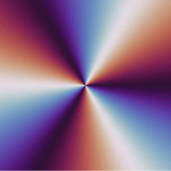
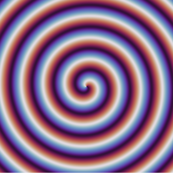
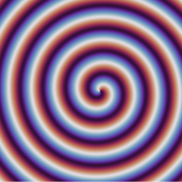
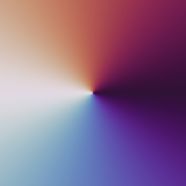
Mapping function $f$						Network architecture:
	(a) $x\in\mathbb{R}\rightarrow e^{ix}$	(b) $x\in\mathbb{C}\rightarrow e^{3i\arg(x)}$	(c) $x\in\mathbb{C}\rightarrow e^{i(\arg(x)+5|x|)}$	(d) $x\in\mathbb{C}\rightarrow{e^{i(\arg(x-o)+5|x-o|)}}$	(e) $x\in\mathbb{C}\rightarrow x/|x|$
Connected pre-images	✗	✗	✓	✓	✓
Convex pre-images	✗	✗	✗	✗	✓
Training set representations $x$
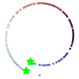
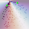
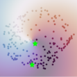
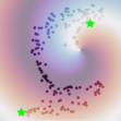
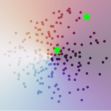
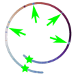
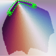
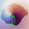
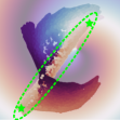
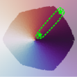
Test set representations $x$						Target predictions†:
Test set hue predictions†

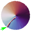
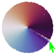
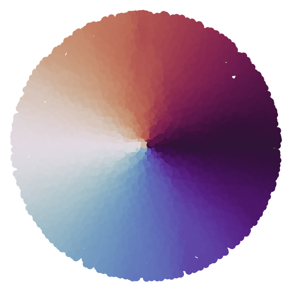
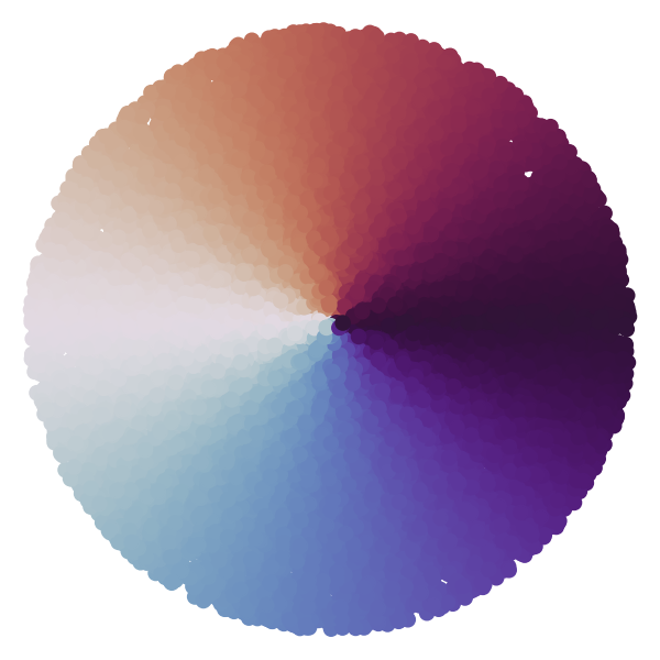
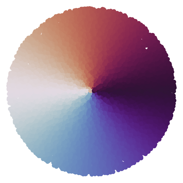
(a): 1D representation is plotted on an Archimedean spiral for visualization purposes. (d): $o$ represents a 2D offset.
$(\dagger)$: Inputs (RGB values of constant lightness) are represented as points on the hue-saturation chromatic disk, with a color corresponding to the predicted hue.

Figure 1: Pre-images connectivity/convexity helps generalization. We train a network to regress color hues from RGB values. It maps the output of a MLP backbone to the hue circle $Y$ using a function $f$. Colors displayed correspond to predicted hues. Training can lead the backbone to produce distant representations for training samples sharing a similar hue $y^{*}$ (green stars, 4^th row). If these representations are in disconnected regions of the pre-image $f^{-1}(y^{*})$, the network will not be able to properly interpolate between them (a,b, green marks, last two rows). Pre-images connectivity guarantees that there exists a continuous backbone function able to interpolate between such training samples (c), but it can be hard to learn in practice (d). Pre-images convexity (e) provides stronger guarantees and tends to help generalization.

2.2 Softmax example

Multiple classical deep learning operators are related to this notion of differentiable mapping, and as an example we show how softmax used in classification can be thought of as a function mapping elements of $X=\mathbb{R}^{n}$ to a probability distribution in $Y=\{(p_{i})_{i=1\ldots n}\in]0,1[^{n}|\sum_{i}p_{i}=1\}$. $Y$ is a connected $(n-1)$-dimensional differentiable manifold on which softmax is surjective. Softmax $i$-th component $p_{i}$ for a vector $(x_{1},\ldots,x_{n})$ is defined by $p_{i}=\exp(x_{i})/{\sum_{j}\exp(x_{j})}$. It is differentiable with partial derivatives ${\partial p_{i}}/{\partial x_{j}}=[p_{i}(1-p_{j})\text{ if }i=j,-p_{i}p_{j}\text{ else}].$ The pre-image of any $(p_{i})_{i=1\ldots n}\in Y$ is the convex line $\operatorname{softmax}^{-1}((p_{i})_{i=1\ldots n})=\left\{\log(p_{i})_{i=1\ldots n}+c|c\in\mathbb{R}\right\}.$ Therefore, for an arbitrary vector $\bm{x}=(x_{i})_{i=1\ldots n}$, one can choose a given $c\in\mathbb{R}$ such as $\log(\operatorname{softmax}(\bm{x}))+c=\bm{x}$, applying $\log$ element-wise. The differentiable function $g:\bm{p}\in Y\rightarrow\log(\bm{p})+c$ can be seen as an inverse of the restriction of $f$ to $g(Y)$, forming a diffeomorphism between $Y$ and $g(Y)$ and therefore guaranteeing the Jacobian of $f$ at $\bm{x}$ to be of same rank as the dimension of $Y$.

3 Differentiable mappings on SO(3)

Based on the theoretical considerations developed in section 2, we review differentiable functions used in the literature to map arbitrary Euclidean vectors to the 3D rotation space. Table 1 provides a short summary of how these different mappings satisfy the properties listed in section 2, and we provide proofs in the supplementary material.

Table 1: Satisfaction of properties of section 2 by $SO(3)$ mappings.

	Domain	Surjective/ differentiable	Full rank Jacobian	Connected/convex pre-images
Euler angles	$\mathbb{R}^{3}$	✓	✗	✗
Rotation vector	$\mathbb{R}^{3}$	✓	✗	✗
Quaternion	$\mathbb{R}^{4}\setminus\{\bm{0}\}$	✓	✓	✗
6D	$\mathcal{M}_{3,2}(\mathbb{R})^{\dagger}$	✓	✓	✓
Procrustes	$\mathcal{M}_{3,3}(\mathbb{R})^{\dagger}$	✓	✓	✓
Symmetric matrix	${\mathbb{R}^{10}}^{\dagger}$	✓	✓	✓

$(\dagger)$: defined on all but a null-measure subset of the domain.

Euler angles

Euler [7] showed that the orientation of any rigid body could be expressed by 3 angles describing a succession of 3 rotations around elementary axes (the choice of which being a matter of convention). As an example, one can consider a succession of rotations around respectively the $x-y-z$ axes and define a mapping $(\alpha,\beta,\gamma)\in\mathbb{R}^{3}\rightarrow\bm{R}_{x}(\alpha)\bm{R}_{y}(\beta)\bm{R}_{z}(\gamma)\in SO(3).$ While being surjective, it does not satisfy pre-images connectivity in general due to the existence of multiple discrete pre-images for a given rotation, and its Jacobian suffers from rank deficiency for some rotations (phenomenon referred to as gimbal lock). Zhou et al. [31] e.g. predict a 3D translation vector and a rotation parameterized by 3 Euler angles, latter cast into a rigid transformation matrix as part of their unsupervised training strategy.

Rotation vector

Rotation vector space can be seen as an unrolling of the rotation space on a tangent plane of the identity rotation. Any arbitrary 3D vector can be mapped to the rotation space through the exponential map (e.g. using Rodrigues’ formula), which consists in a surjective function over the rotation space. However, similarly to Euler angles it suffers from multiple discrete pre-images, and rank deficiency for input rotation vectors of angle $2\pi k,k\in\mathbb{N}^{*}$. It is used e.g. in [27] to regress parameters of a human model. Note however that a restriction from an open ball of radius $\alpha<\pi$ to the set of rotations of angle strictly smaller than $\alpha$ satisfies all properties of section 2, and that such mapping is therefore suited to regress rotations of limited angles.

Non zero quaternion

The rotation group $SO(3)$ is diffeomorphic to $\mathbb{RP}^{3}$ [8] and therefore one can define a mapping from $X=\mathbb{R}^{4}\setminus\{\bm{0}\}$ to $SO(3)$ by considering each element $\bm{x}\in X$ as a representation of a rotation parameterized by a unit norm quaternion $\bm{q}=\bm{x}/\|\bm{x}\|$. Such mapping satisfies all but pre-images connectivity constraint as the pre-image of any rotation parameterized by a non zero quaternion $\bm{q}$ consists in $\{\alpha\bm{q}|\alpha\in\mathbb{R}^{*}\}$ which is not connected. This mapping is used e.g. in PoseNet [16], and Liao et al. [19] suggest a variant of this mapping to stabilize training.

Procrustes

An arbitrary $3\times 3$ matrix $\bm{M}$ can be projected to the closest rotation matrix considering Frobenius norm by solving the special orthogonal Procrustes problem $\operatorname{Procrustes}(\bm{M})=\arg\min_{\bm{\tilde{R}}\in SO(3)}\|\bm{\tilde{R}}-\bm{M}\|_{F}^{2}.$ Solutions to this minimization problem can be expressed $\bm{U}\bm{S}\bm{V}^{\top}$ [28, 29], where $\bm{U}\bm{D}\bm{V}^{\top}$ is a singular value decomposition of $\bm{M}$ such that $\bm{U},\bm{V}\in O(d)$, $\bm{D}=\operatorname{diag}(\alpha_{1},\alpha_{2},\alpha_{3})$ is a diagonal matrix satisfying $\alpha_{1}\geq\alpha_{2}\geq\alpha_{3}\geq 0$ and $\bm{S}$ is defined by $\operatorname{diag}(1,1,\det(\bm{U})\det(\bm{V}))$. The solution is actually unique if $\det(\bm{M})>0$ or $\alpha_{2}\neq\alpha_{3}$, and Procrustes mapping is therefore well-defined almost everywhere on the set of $3\times 3$ matrices, but on a set of null measure (usually ignored in practice). We show in the supplementary material that it satisfies all properties presented in section 2, notably that the pre-image of any rotation is convex. Procrustes mapping is therefore a suitable candidate for reliable learning, and it can be implemented efficiently for batched GPU applications using off-the-shelf SVD cuSOLVER routines. It is used e.g. in [22] for human pose estimation, and some concurrent work [18] advocates for its use as a universally effective representation.

6D

Zhou et al. [32] proposed a similar approach consisting in mapping a $3\times 2$ matrix $\bm{M}$ (6D in total) to a rotation matrix through Gram-Schmidt orthonormalization. We show in supplementary material that this process can be thought of as a degenerate case of Procrustes orthonormalization, expressed as a limit

$$\operatorname{6D}(\bm{M})=\lim_{\alpha\rightarrow 0^{+}}\arg\min_{\bm{R}\in SO(3)}\|\bm{R}\left(\begin{smallmatrix}1&0\\ 0&\alpha\\ 0&0\end{smallmatrix}\right)-\bm{M}\|_{F}^{2}.$$ (1)

Solving this optimization problem for a given $\alpha>0$ is equivalent to solving the Procrustes one, considering $\bm{M}\left(\begin{smallmatrix}1&0&0\\ 0&\alpha&0\end{smallmatrix}\right)\in\mathcal{M}_{3,3}(\mathbb{R})$ as input. Both mappings therefore share in that sense similar properties, except that the 6D mapping gives importance almost exclusively to the first column of $\bm{M}$ and is only well-defined when $\operatorname{rank}(\bm{M})=2$. Zhou et al. [32] showed that this 6D representation could actually be compressed into a 5D one through the use of stereographic projection, which led to worse training performances in practice. We show in supplementary material how this mapping satisfies properties of section 2. The 6D mapping is used in various recent papers [24, 17], but experiments of [18] and ours suggest that it is generally outperformed by Procrustes orthonormalization.

Symmetric matrix Lastly, Peretroukhin et al. [25] recently proposed to regress 3D rotations as a list of 10 coefficients of a $4\times 4$ symmetric matrix $\bm{A}$, and showed that one could map such matrix to a unique rotation (expressed as a unit quaternion) associated with a particular probability distribution, as long as the smallest eigenvalue of $\bm{A}$ has a multiplicity of 1. We show in the supplementary material how it also satisfies the properties of section 2.

RoMa library

Writing code handling various rotation representations and mappings can be hard and error-prone because of the multiple corner-cases to consider. To ease deep learning experiments involving these rotation mappings, we release RoMa (https://naver.github.io/roma/) – an easy-to-use and efficient PyTorch library for rotation manipulation, and hope it will support future research.

4 Experiments

We report in this section a methodological performance evaluation of $SO(3)$ mappings on a variety of tasks, namely point cloud alignment (sec. 4.1), inverse kinematics (sec. 4.2), camera localization (sec. 4.3) and object pose estimation (sec. 4.4). More precisely, we present in sections 4.1 and 4.2 a reproduction and extension of experiments of [32] including an additional mapping Procrustes, and a study of the results variance across multiple trainings. Benchmarks proposed in sections 4.3 and  4.4 consists in novel tasks.

The goal of these experiments is twofold: 1) test the relevance of properties proposed in section 2 regarding what makes a good mapping, and 2) provide a performance comparison of $SO(3)$ mappings on a variety of tasks.

We did not include Euler angles in our experiments as many different conventions would have to be considered. Similarly, we ignored the mapping based on a $4\times 4$ symmetric matrix representation [25], as its implementation was found too slow to be used in extensive evaluations. When the loss function is expressed directly as a distance in $3\times 3$ matrix space (sections 4.1 and 4.4), we additionally evaluate variants consisting in regressing an arbitrary $3\times 3$ matrix at training time using this particular loss, and performing the mapping on SO(3) only at test time (we refer to these variants as Matrix/Procrustes and Matrix/Gram-Schmidt depending on the mapping used at test time).

4.1 Point cloud alignment

We reproduce and extend the experiment of [32] on point clouds alignment, which while being artificial, provides an interesting benchmark. Given an input 3D point cloud $C_{1}=\{\bm{x}_{i}\}_{i=1\ldots n}$ of size $n$ (with $\bm{x}_{i}\in\mathbb{R}^{3}$), and a copy $C_{2}=\{r^{*}(\bm{x}_{i})\}_{i=1\ldots n}$ rotated by a random rotation $r^{*}\in SO(3)$, we train a neural network to regress this rotation. The network consists of two Siamese naive PointNets returning a feature vector for each point cloud, which are concatenated and passed through a multi-layer perceptron to produce a feature vector mapped to a rotation $r$ using one of the mappings studied. Consistently with Zhou et al., training is performed by minimizing the square Frobenius distance between rotation matrices $\bm{R},\bm{R}^{*}\in\mathcal{M}_{3,3}(\mathbb{R})$ representing these rotations $r$ and $r^{*}$: $\mathcal{L}(r,r^{*})=\|\bm{R}-\bm{R}^{*}\|_{F}^{2}$.

Protocol

We follow the protocol of [32], using the dataset provided by the authors representing airplanes from ShapeNet [5]. We select however randomly a validation set of 400 point clouds from the original training set, and randomly subsample point clouds to a size of 1024. We run the experiment with various mappings to the rotation space and report results in table 2 and figure 2. Due to the stochastic nature of training, we train/test each variant 5 times and aggregate results to mitigate their variance and increase confidence in our findings. More precisely, we report the error for the model having obtained the smallest validation error (being checked after each training epoch), as well as the final error obtained at the end of training, averaged over 5 runs.

Table 2: Mean angular error on test set for point cloud alignment, aggregated across 5 independent trainings (lower is better).

Subscript and exponent represent the min. and max. deviations from the average. Method Best validation Average final error (°) Rotation vector $12.74\degree{}$ $14.27_{-0.84}^{+1.32}$ Quaternion $11.66\degree{}$ $12.99_{-1.13}^{+1.49}$ 6D $3.01\degree{}$ $3.47_{-0.45}^{+0.45}$ Procrustes $\bm{2.90\degree}$ $\bm{3.46}_{-0.35}^{+0.59}$ Matrix/Gram-Schmidt $3.66\degree$ $4.07_{-0.10}^{+0.21}$ Matrix/Procrustes $\bm{3.33\degree}$ $\bm{3.59}_{-0.09}^{+0.08}$

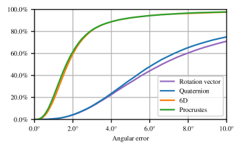
Figure 2: Cumulative angular error distribution on test set for point cloud alignment (best validation models only, for readability).

Results

In accordance with the results reported in [32], rotation vector and quaternion mappings achieve significantly worse performances than the other mappings. Procrustes orthonormalization leads to better results than Gram-Schmidt one, both during training (Procrustes vs. 6D), and when used only at test time (Matrix/Procrustes vs. Matrix/Gram-Schmidt). Difference of average final error between Procrustes and 6D is too small however to draw clear conclusions from this metric alone, given the deviations observed across the different runs.

Interestingly, we achieve better performance when performing orthonormalization both at training and test time (6D and Procrustes) compared to regressing a raw matrix and performing orthonormalization only for validation/test (Matrix/Gram-Schmidt and Matrix/Procrustes). However, we observe a smaller final error variance when training without orthonormalization, with a maximum deviation of 0.18° for Matrix/Procrustes vs. 0.91° for Procrustes, and 0.31° for Matrix/Gram-Schmidt vs. 0.89° for 6D. We explain this by the fact that learning is more constrained in the direct regression scenario.

4.2 Inverse kinematics

We reproduce and extend another experimental setup of [32], more representative of a real use case, and where rotation regression is trained in a self-supervised manner.

The problem consists in learning an inverse kinematic model of a human skeleton from a set of recorded motions. The forward kinematic function $f$ mapping the $n=57$ rotations $(r_{i})_{i=1\ldots n}\in SO(3)^{n}$ associated to each joint to their 3D locations $(\bm{x}_{i})_{i=1\ldots n}\in\mathbb{R}^{3\times n}$ is assumed to be known. We train a multi-layer perceptron $g:\mathbb{R}^{3\times n}\rightarrow SO(3)^{n}$ to regress the inverse mapping. During training, given a target list of 3D joints locations $(\bm{x}^{*}_{i})_{i=1\ldots n}$, we use an auto-encoding approach regressing a list of joints locations $(\bm{x}_{i})_{i=1\ldots n}=f(g((\bm{x}^{*}_{i})_{i=1\ldots n})$, and train the network to minimize the square residual $\sum_{i=1}^{n}\alpha_{i}\|\bm{x}_{i}-\bm{x}^{*}_{i}\|^{2}$.

Protocol

We follow closely the protocol of [32] and use data provided by the authors from the CMU MoCap Database [4]. We select randomly 73 training sequences as validation set, and train each variant with 5 different random weight initializations to assess the confidence of our observations.

Results

We report results in table 3 and figure 3. The Procrustes and 6D mappings greatly outperform the others in this experiment, with Procrustes showing significantly better performances than 6D.

Table 3: Mean per joint position error on the inverse kinematics test set, aggregated across 5 independent trainings (lower is better).

Subscript and exponent represent the min. and max. deviations from the average. Method Best validation Average final error (cm) Quaternion 1.948cm $2.208_{-0.241}^{+0.208}$ Rotation vector 1.695cm $1.840_{-0.144}^{0.102}$ 6D 0.796cm $0.885_{-0.079}^{+0.103}$ Procrustes 0.721cm $\bm{0.795}_{-0.061}^{+0.088}$

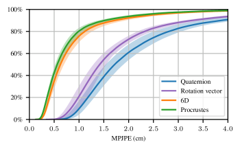
Figure 3: Cumulative mean per joint error distribution on the inverse kinematics test set, aggregated across 5 independent trainings (Solid line: average distribution, shaded areas: maximal deviation across runs).

4.3 Camera localization

We study the impact of mapping function on the problem of absolute 6D camera localization, and base our experiments on PoseNet [16], a pioneer work of image-based direct camera pose regression. PoseNet processes an input RGB image using a CNN to regress the camera pose from which the image was taken, after a prior supervised training. In its original version, camera pose is regressed as a pair $(\bm{t},\bm{q})$ composed of a translation vector $\bm{t}\in\mathbb{R}^{3}$ and a unit quaternion $\bm{q}\in\mathbb{R}^{4}$ obtained by normalizing an arbitrary 4D output of a neural network. Given a ground truth pose $(\bm{t}^{*},\bm{q}^{*})$, original training aims to minimize the loss function

$$\mathcal{L}_{original}=\alpha\|\bm{t}-\bm{t}^{*}\|^{2}+\beta\gamma\|\bm{q}-\bm{q}^{*}\|^{2},$$ (2)

with $\alpha=1/3$, $\gamma=1/4$ and where $\beta$ is a scaling factor weighting the importance of rotation vs. translation.

Protocol

We replace the last fully connected layer of the network to produce a feature vector of adequate dimension to apply each evaluated mapping and regress a rotation. Rotation part of the original loss function (2) is actually biased as it is not a valid similarity measure on $SO(3)$. Indeed, a 3D rotation can be represented by two antipodal unit quaternions $\bm{q}$ and $-\bm{q}$, therefore one should instead consider

$$\mathcal{L}_{quaternion}=\alpha\|\bm{t}-\bm{t}^{*}\|^{2}+\beta\gamma\min\|\bm{q}\pm\bm{q}^{*}\|^{2}$$ (3)

in order to avoid border effects of the representation.

To investigate the impact of the training loss function on the results, we also experiment to replace it by one based on Frobenius distance between rotation matrices $\bm{R},\bm{R}^{*}$

$$\mathcal{L}_{Frobenius}=\alpha\|\bm{t}-\bm{t}^{*}\|^{2}+\beta\delta\|\bm{R}-\bm{R}^{*}\|_{F}^{2}.$$ (4)

We choose $\delta=\gamma/8$ to weight the losses similarly (see supp. mat. for details). We evaluate variants of PoseNet on Cambridge Landmarks datasets, and report median camera position and orientation errors. We use the PoseNet implementation of Walch et al. [30] with its recommended hyperparameters settings. We observed negligible variance in the results across different training, because of the use of pre-trained weights and deterministic seeding, and we therefore report a single result for each mapping.

Results

The results obtained are summarized in table 4.

Table 4: Median camera localization error on Cambridge Landmarks datasets.

Loss	$\mathcal{L}_{original}$	$\mathcal{L}_{quaternion}$ (loss (3))					$\mathcal{L}_{Frobenius}$ (loss (4))
Representation	quaternion	quaternion	Rot-vec	6D	Procrustes	Rot-vec 180°	quaternion	Rot-vec	6D	Procrustes
KingsCollege	1.54m, 4.25°	1.82m, 4.73°	1.64m, 4.77°	1.64m, 4.82°	1.46m, 5.15°	1.51m, 138.01°	1.87m, 4.98°	1.57m, 4.87°	1.70m, 4.56°	1.87m, 5.17°
OldHospital	2.64m, 5.20°	2.36m, 5.15°	1.95m, 5.88°	2.52m, 4.90°	2.23m, 4.63°	2.32m, 155.73°	2.53m, 5.23°	2.56m, 4.97°	2.68m, 4.83°	2.37m, 4.39°
ShopFacade	2.04m, 10.07°	2.21m, 10.49°	1.44m, 9.68°	2.40m, 10.61°	1.57m, 8.25°	1.55m, 143.32°	2.16m, 9.56°	1.27m, 7.55°	1.90m, 9.22°	1.50m, 8.75°
StMarysChurch	2.06m, 7.45°	2.21m, 10.13°	1.94m, 7.88°	2.22m, 8.17°	2.11m, 8.08°	2.02m, 165.23°	1.97m, 8.32°	2.02m, 7.82°	2.14m, 8.01°	2.01m, 7.28°
Mean	2.07m, 6.74°	2.15m, 7.63°	1.74m, 7.05°	2.19m, 7.13°	1.84m, 6.53°	1.85m, 150.57°	2.13m, 7.02°	1.85m, 6.30°	2.10m, 6.65°	1.94m, 6.40°

The baseline quaternion mapping trained with the original loss (2) performs well compared to the variants trained with the quaternion loss (3). It is not totally surprising in the sense that hyperparameters have been tuned for this particular setting, introducing a bias in its favor. It notably performs better on average than the quaternion mapping trained using loss (3), despite the fact the former is ill-defined on $SO(3)$ as described previously. We conjecture that it might be due to the combination of two factors. First, loss (3) might be confusing during training and lead to poorer generalization than loss (2) when using a quaternion representation because 4D outputs of the backbone network corresponding to nearby orientations may be pushed towards different and opposite regions with this loss (this relates to the fact that the quaternion mapping does not satisfy the pre-images connectivity property). Second, ground truth unit quaternions representations $\bm{q}^{*}$ are oriented consistently in the dataset. For each dataset more than 99% of ground truth quaternions are indeed oriented in the same half-space, mostly far from its border, which mitigates the potential border effects introduced by loss (2).

Results obtained using the Procrustes representation are globally better than those using the 6D or quaternion representations for both losses (3) and (4), and are on average better than the baseline.

The rotation vector representation performed surprisingly well in this experiment despite the fact that this mapping does not satisfy the criteria of section 2, even achieving the best average results for loss (4). We conjecture that this success might be due to a combination of a ‘lucky’ weight initialization and to the fact that rotations to regress in the datasets are typically less than 90° away from the identity, enabling the use of a portion of the rotation vector space in which properties of section 2 are roughly met (a similar hypothesis was studied in [23] for non-monotonic activation functions). We tested this hypothesis by applying to the regressed rotation a 180° rotation around the $x$ camera axis before the evaluation of the loss, in such a way that poses to regress are no longer close to the identity. Training completely failed to converge to a good solution as reported in table 4 for loss (3), which supports our hypothesis. It did however succeed for loss (4), reaching performances of the order of those of the non-rotated version.

4.4 Object pose estimation

Lastly, we investigate the impact of the mapping function on object pose estimation from an RGB image.

Protocol

We try to predict the 3D orientation of a rigid object from an image crop extracted from LINEMOD dataset [11]. Following a common practice [26], we use synthetic data for training, rendering 200,000 crops for each object with randomized pose, illumination and background. For the sake of simplicity, we do not use any real data, physically-based renderings, or data-augmentation during training and cannot therefore pretend reaching the same level of performances than state-of-the-art methods [13]. We use for each object a pre-trained ResNet-50 backbone [9], and replace the last fully connected layer by one whose output dimension is suitable for the mapping considered. We freeze the first layers of the backbone (up to the second one) to speed up the training and following insights from [12] regarding generalization performances. Given a ground truth object orientation expressed as a rotation $r^{*}\in SO(3)$, we train the model to regress a rotation $r\in SO(3)$ minimizing the mean square position error of the object’s surface points

$$\mathcal{L}(r,r^{*})=\cfrac{1}{d^{2}S}\int_{\mathcal{S}}{\|r(\bm{x})-r^{*}(\bm{x})\|^{2}ds},$$ (5)

where $\mathcal{S}$ represents the surface of the object expressed in a coordinate system centered on its centroid, $S$ its area and where $d$ is a normalizing factor corresponding to the diameter of the object. We showed in [1] that this loss function admits a closed-form solution $\|(\bm{R}-\bm{R}^{*})\bm{\Lambda}\|_{F}^{2}$, where $\bm{\Lambda}$ is a symmetric positive matrix depending on the object. We train the network for 30 epochs using SGD and perform hyperparameters search on the validation set (see supp. mat. for details). At test time, we report the mean RMS error regarding the position of the surface points.

Results

The results are summarized in table 5. The Procrustes and 6D mappings achieve better results than the quaternion and rotation vector ones, and Procrustes outperforms 6D for most objects. Training to regress an arbitrary $3\times 3$ matrix without special orthonormality constraints leads to worse performances at test time, but Procrustes orthonormalization still outperforms Gram-Schmidt in this scenario.

Table 5: Regression of object orientation from an image. Mean RMS error normalized by the object diameter (lower is better).

Object	Quat.	Rot-vec	6D	Procr.	Mat/GS.	Mat/Procr.
ape	0.145	0.119	0.085	0.080	0.109	0.107
bench vise	0.062	0.068	0.049	0.042	0.067	0.069
camera	0.139	0.145	0.084	0.067	0.236	0.130
watering can	0.162	0.169	0.134	0.132	0.242	0.239
cat	0.078	0.091	0.048	0.049	0.174	0.111
cup	0.215	0.237	0.219	0.221	0.260	0.232
driller	0.106	0.089	0.059	0.048	0.186	0.144
duck	0.100	0.118	0.050	0.051	0.135	0.129
hole puncher	0.177	0.165	0.137	0.126	0.218	0.176
iron	0.051	0.053	0.041	0.037	0.055	0.079
lamp	0.061	0.054	0.032	0.035	0.088	0.081
phone	0.101	0.129	0.073	0.077	0.155	0.122
Mean	0.116	0.120	0.084	0.080	0.160	0.135

5 Discussion

In this section, we try to derive some general insights from the results of our experiments.

Theory validation We globally observed better results with the Procrustes and 6D mappings than with the ones based on quaternion and rotation vectors. This is consistent with the theory developed in section 2 regarding what properties should satisfy a mapping to enable good training and generalization. In the camera localization experiment, the drop of performance observed with the quaternion mapping when switching from the original PoseNet loss (2) to a well-defined loss on the rotation space (3) supports the idea that the non-connectivity of pre-images is a problem for learning. It is somehow also supported by the failure to converge to a low error solution observed with the Rot-vec 180° representation. We tested our theory on several manifolds – $\mathbb{S}^{1}$, $SO(3)$, $SO(3)^{n}$, and $SE(3)$ (resp. in fig. 1, sections 4.1 and 4.4, 4.2, 4.3) – and we also report supporting results on a torus as supplementary material.

Mapping ‘linearity’ We also observed that regressing a $3\times 3$ matrix and performing Procrustes orthonormalization at training time globally performed better than using the 6D representation. Work concurrent to ours [18] led to similar conclusions and provides two arguments. The first consists in the smaller sensitivity of Procrustes orthonormalization to Gaussian noise compared to Gram-Schmidt, but their results only hold for local perturbations applied to a rotation matrix. The second is that Procrustes orthonormalization is left- and right-invariant to rotations, whereas Gram-Schmidt is only left-invariant (we discussed in section 3 how 6D gives more importance to the first input column vector). We propose here as another explanation that the Procrustes mapping is more ‘linear’ than 6D and quaternion for typical input ranges, and we support this claim by numerical experiments. We draw for each mapping $\bm{R}:\bm{x}\in\mathbb{R}^{n}\rightarrow\bm{R}(\bm{x})\in SO(3)$ some random input vector $\bm{x}\sim\mathcal{N}(0,1)^{n}$, as well as some unit 3D vectors $\bm{v}_{1},\bm{v}_{2}$ of uniform random direction. Because of the way Procrustes, 6D and quaternion mappings are defined, $\bm{R}(\bm{x})$ is uniformly distributed over $SO(3)$ and no bias is introduced by this approach. We define a loss function $\mathcal{L}(\bm{x})=\bm{v}_{1}^{T}\bm{R}(\bm{x})\bm{v}_{2}$, estimate its gradient $\nabla\mathcal{L}_{\bm{x}}$ and compute for a given step size $\epsilon>0$ the absolute deviation from the linear case: $|\mathcal{L}(\bm{x}-\epsilon\nabla\mathcal{L}_{\bm{x}})-(\mathcal{L}(\bm{x})-\epsilon\|\nabla\mathcal{L}_{\bm{x}}\|^{2})|$. Results for various step sizes are plotted in fig. 4 and show the better linearity of Procrustes compared to quaternion and 6D.

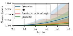
Curve corresponding to Rotation vector is masked by Procrustes.

Figure 4: Deviation from linearity of different mappings on SO(3) (solid curves: median, shaded areas: 25%-75% percentiles).

Direct/surrogate objective We also observed that using a differentiable mapping $\bm{x}\rightarrow f(\bm{x})$ at training time and defining a loss on the target manifold performed better in our experiments than training to regress a representation $\bm{x}$, and mapping it to the manifold at test time (e.g. Procrustes vs. Matrix/Procrustes). This seems a natural finding as we optimize in the former case an objective function corresponding to our actual goal defined on the manifold, whereas the latter case considers only a surrogate objective in the representation space.

Small rotation vector Finally, our experiments with PoseNet showed that a rotation vector mapping could perform well in some circumstances, and notably when considering rotations of limited angle. Such mapping actually satisfies the criteria of section 2 when restricted from a unit ball of radius $\alpha\in]0,\pi[$ to the corresponding set of rotations, and the plot in figure 4 indeed suggests a linearity similar between Procrustes and the mapping to rotations of angle strictly smaller than $\pi/2$

$$\bm{x}\in\mathbb{R}^{3}\rightarrow\exp(\cfrac{\pi}{2}\tanh(\|\bm{x}\|)\cfrac{\bm{x}}{\|\bm{x}\|})$$ (6)

for normal inputs.

6 Conclusion

In this paper, we study the problem of deep regression on a manifold through the use of a mapping from the Euclidean output space of a neural network to this manifold. We establish a list of properties that such mapping should satisfy to allow a proper gradient-based training, and highlight in particular the importance of pre-images connexity/convexity. We review the specific case of the 3D rotation manifold, considering existing mappings both from a theoretical and experimental standpoint, and conjecture that linearity of the mapping might be an important additional aspect to achieve good performances. We show that a mapping based on special Procrustes orthonormalization performs best among the mappings considered when regressing arbitrary rotations, but that rotation-vector representations may be as suitable when the output can be constrained to limited rotation angles.

References

- [1] Romain Brégier, Frédéric Devernay, Laetitia Leyrit, and James L. Crowley. Defining the Pose of Any 3D Rigid Object and an Associated Distance. International Journal of Computer Vision, 2018.
- [2] Michael M. Bronstein, Joan Bruna, Yann LeCun, Arthur Szlam, and Pierre Vandergheynst. Geometric deep learning: going beyond Euclidean data. IEEE Signal Processing Magazine, 2017.
- [3] W. Cao, Z. Yan, Z. He, and Z. He. A Comprehensive Survey on Geometric Deep Learning. IEEE Access, 2020.
- [4] CMU Graphics Lab Motion Capture Database. http://mocap.cs.cmu.edu.
- [5] Angel X. Chang, Thomas Funkhouser, Leonidas Guibas, Pat Hanrahan, Qixing Huang, Zimo Li, Silvio Savarese, Manolis Savva, Shuran Song, Hao Su, Jianxiong Xiao, Li Yi, and Fisher Yu. ShapeNet: An Information-Rich 3D Model Repository. Technical Report arXiv:1512.03012 [cs.GR], 2015.
- [6] Alberto Crivellaro, Mahdi Rad, Yannick Verdie, Kwang Moo Yi, Pascal Fua, and Vincent Lepetit. A novel representation of parts for accurate 3d object detection and tracking in monocular images. In ICCV, 2015.
- [7] Leonhard Euler. Formulae generales pro translatione quacunque corporum rigidorum. Euler Archive - All Works by Eneström Number, 1776.
- [8] Brian C. Hall. Lie Groups, Lie Algebras, and Representations: An Elementary Introduction, Graduate Texts in Mathematics, 222 (2nd ed.). Springer, 2015.
- [9] Kaiming He, Xiangyu Zhang, Shaoqing Ren, and Jian Sun. Deep residual learning for image recognition. In CVPR, 2016.
- [10] Yisheng He, Wei Sun, Haibin Huang, Jianran Liu, Haoqiang Fan, and Jian Sun. PVN3D: A Deep Point-Wise 3D Keypoints Voting Network for 6DoF Pose Estimation. In CVPR, 2020.
- [11] Stefan Hinterstoisser, Stefan Holzer, Cedric Cagniart, Slobodan Ilic, Kurt Konolige, Nassir Navab, and Vincent Lepetit. Multimodal templates for real-time detection of texture-less objects in heavily cluttered scenes. In ICCV, 2011.
- [12] Stefan Hinterstoisser, Vincent Lepetit, Paul Wohlhart, and Kurt Konolige. On Pre-Trained Image Features and Synthetic Images for Deep Learning. In ECCV, 2018.
- [13] Tomas Hodan, Martin Sundermeyer, Bertram Drost, Yann Labbe, Eric Brachmann, Frank Michel, Carsten Rother, and Jiri Matas. BOP Challenge 2020 on 6D Object Localization. In ECCVW, 2020.
- [14] Asako Kanezaki, Yasuyuki Matsushita, and Yoshifumi Nishida. RotationNet: Joint Object Categorization and Pose Estimation Using Multiviews from Unsupervised Viewpoints. In CVPR, 2018.
- [15] Wadim Kehl, Fabian Manhardt, Federico Tombari, Slobodan Ilic, and Nassir Navab. SSD-6D: Making RGB-Based 3D Detection and 6D Pose Estimation Great Again. In ICCV, 2017.
- [16] Alex Kendall, Matthew Grimes, and Roberto Cipolla. PoseNet: A convolutional network for real-time 6-DOF camera relocalization. In ICCV, 2015.
- [17] Muhammed Kocabas, Nikos Athanasiou, and Michael J. Black. VIBE: Video Inference for Human Body Pose and Shape Estimation. In CVPR, 2020.
- [18] Jake Levinson, Carlos Esteves, Kefan Chen, Angjoo Kanazawa, Afshin Rostamizadeh, Noah Snavely, and Ameesh Makadia. An Analysis of SVD for Deep Rotation Estimation. In NeurIPS, 2020.
- [19] Shuai Liao, Efstratios Gavves, and Cees G. M. Snoek. Spherical Regression: Learning Viewpoints, Surface Normals and 3D Rotations on n-Spheres. In CVPR, 2019.
- [20] D. Mohlin, G. Bianchi, and J. Sullivan. Probabilistic orientation estimation with matrix Fisher distributions. NeurIPS, 2020.
- [21] Kieran Murphy, Carlos Esteves, Varun Jampani, Srikumar Ramalingam, and Ameesh Makadia. Implicit-PDF: Non-Parametric Representation of Probability Distributions on the Rotation Manifold. In ICML, 2021.
- [22] Mohamed Omran, Christoph Lassner, Gerard Pons-Moll, Peter V. Gehler, and Bernt Schiele. Neural Body Fitting: Unifying Deep Learning and Model-Based Human Pose and Shape Estimation. In 3DV, 2018.
- [23] Giambattista Parascandolo, Heikki Huttunen, and Tuomas Virtanen. Taming the waves: sine as activation function in deep neural networks. 2016.
- [24] Georgios Pavlakos, Nikos Kolotouros, and Kostas Daniilidis. TexturePose: Supervising Human Mesh Estimation with Texture Consistency. In ICCV, 2019.
- [25] Valentin Peretroukhin, Matthew Giamou, David M. Rosen, W. Nicholas Greene, Nicholas Roy, and Jonathan Kelly. A Smooth Representation of Belief over SO(3) for Deep Rotation Learning with Uncertainty. In Robotics: Science and Systems XVI, 2020.
- [26] Mahdi Rad and Vincent Lepetit. BB8: A Scalable, Accurate, Robust to Partial Occlusion Method for Predicting the 3D Poses of Challenging Objects without Using Depth. In ICCV, 2017.
- [27] Yu Rong, Ziwei Liu, Cheng Li, Kaidi Cao, and Chen Change Loy. Delving Deep Into Hybrid Annotations for 3D Human Recovery in the Wild. In ICCV, 2019.
- [28] Peter H. Schönemann. A generalized solution of the orthogonal Procrustes problem. Psychometrika, 1966.
- [29] Shinji Umeyama. Least-squares estimation of transformation parameters between two point patterns. TPAMI, 1991.
- [30] F. Walch, C. Hazirbas, L. Leal-Taixe, T. Sattler, S. Hilsenbeck, and D. Cremers. Image-Based Localization Using LSTMs for Structured Feature Correlation. In ICCV, 2017.
- [31] Tinghui Zhou, Matthew Brown, Noah Snavely, and David G Lowe. Unsupervised Learning of Depth and Ego-Motion From Video. In CVPR, 2017.
- [32] Yi Zhou, Connelly Barnes, Jingwan Lu, Jimei Yang, and Hao Li. On the Continuity of Rotation Representations in Neural Networks. In CVPR, 2019.