Higher-Order Neighborhood Truss Decomposition

Abstract

$k$-truss model is a typical cohesive subgraph model and has been received considerable attention recently. However, the $k$-truss model only considers the direct common neighbors of an edge, which restricts its ability to reveal fine-grained structure information of the graph. Motivated by this, in this paper, we propose a new model named $(k,\tau)$-truss that considers the higher-order neighborhood ($\tau$ hop) information of an edge. Based on the $(k,\tau)$-truss model, we study the higher-order truss decomposition problem which computes the $(k,\tau)$-trusses for all possible $k$ values regarding a given $\tau$. Higher-order truss decomposition can be used in the applications such as community detection and search, hierarchical structure analysis, and graph visualization. To address this problem, we first propose a bottom-up decomposition paradigm in the increasing order of $k$ values to compute the corresponding $(k,\tau)$-truss. Based on the bottom-up decomposition paradigm, we further devise three optimization strategies to reduce the unnecessary computation. We evaluate our proposed algorithms on real datasets and synthetic datasets, the experimental results demonstrate the efficiency, effectiveness and scalability of our proposed algorithms.

1 Introduction

Graphs have been widely used to represent the relationships of entities in real-world applications Sahu et al. (2017); Yuan et al. (2017); Ouyang et al. (2020). With the proliferation of graph applications, plenty of research efforts have been devoted to cohesive subgraph models for graph structure analysis Chang and Qin (2018). Typical cohesive subgraph models include clique Luce and Perry (1949); Yuan et al. (2018, 2016a); Chen et al. (2020), $k$-clique Luce (1950a), quasi-clique Abello et al. (2002); Pei et al. (2005), $k$-core Liu et al. (2019a); Seidman (1983); Liu et al. (2020a), $k$-truss Cohen (2008); Wu et al. , and $k$-ECC Zhou et al. (2012); Chang et al. (2013).

Among them, the $k$-truss model is a typical cohesive subgraph model and has received considerable attention due to its unique cohesive properties on degree and bounded diameter Wang and Cheng (2012); Huang et al. (2014); Akbas and Zhao (2017); Liu et al. (2020b). Given a graph $G$, for an edge $e=(u,v)$ in $G$, the support of $e$ is defined as the number of direct common neighbors of $u$ and $v$. $k$-truss is the maximal subgraph $G^{\prime}$ of $G$ such that the support of each edge in $G^{\prime}$ is not less than $k-2$ Cohen (2008). Truss decomposition computes the $k$-truss in the graph for all possible $k$ values in $G$.

Figure 1: Part of the collaboration network in DBLP

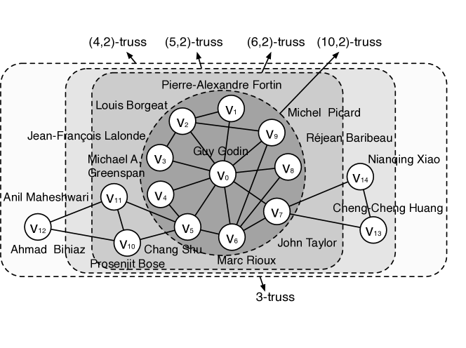
Motivation. Although the $k$-truss model and the corresponding truss decomposition have been successful in many applications, the model lacks the ability to reveal fine-grained structure information of the graph. Consider the graph in Figure 1. Figure 1 shows part of the collaboration network in the DBLP(https://dblp.uni-trier.de/), in which each node represents an author and each edge indicates the co-author relationship between two authors. The results of traditional truss decomposition are shown in Figure 1. The traditional truss decomposition treats the whole graph as a $3$-truss and is not able to provide more fine-grained structure information.

On the other hand, the importance of the higher-order neighborhood (multiple-hop neighbors instead of direct neighbors) on the characterization of complex network has been well established Andrade et al. (2006, 2008), and remarkable results have been obtained in the network science due to the introduction of higher-order neighborhood Abu-El-Haija et al. (2019); Liu et al. (2019b); Bonchi et al. (2019); Xue et al. (2020); Sun et al. (2020). Motivated by this, we propose the $(k,\tau)$-truss model by incorporating the higher-order neighborhood into the $k$-truss model. Formally, given a graph $G$ and an integer $\tau$, for an edge $e=(u,v)$, the higher-order support of $e$ is the number of $\tau$-hop common neighbors of $u$ and $v$. $(k,\tau)$-truss is the maximal subgraph $G^{\prime}$ of $G$ such that the higher-order support of each edge in $G^{\prime}$ is not less than $k-2$. Following the $(k,\tau)$-truss model, we study the higher-order truss decomposition problem that computes the $(k,\tau)$-truss for all possible $k$ values in $G$ regarding a given $\tau$.

The benefits of the $(k,\tau)$-truss model are twofold: (1) it inherits the unique cohesive properties on degree and bounded diameter of $k$-truss, which are shown in Property 3 and Property 3 in Section 3. (2) It acquires the ability to reveal fine-grained structure information due to the introduction of higher-order neighborhood. Reconsider $G$ in Figure 1, Figure 1 shows the higher-order truss decomposition results. By considering the higher-order neighborhood information, the whole graph(3-truss) can be further split into $(4,2)$-truss, $(5,2)$-truss, $(6,2)$-truss and $(10,2)$-truss. The hierarchy structure of the graph is clearly characterized by the higher-order truss decomposition. Note that a cohesive subgraph model named ($k$,$h$)-core that also considers higher-order neighborhood information is studied in Batagelj and Zaveršnik (2011); Bonchi et al. (2019). However, the definition of our model is more rigorous, which makes our model can search “core” of a ($k$,$h$)-core (e.g. a ($k$+1,$\tau$)-truss is a ($k$,$h$)-core but not vice versa,$\tau$=$h$). As shown in our case study (Exp-5), our model has higher ability to reveal fine-grained structure information than ($k$,$h$)-core.

Applications. Higher-order truss decomposition can be applied in the applications using the traditional $k$-truss decomposition since the $k$-truss model is a specific case of $(k,\tau)$-truss model when $\tau=1$, namely $(k,1)$-truss. These applications include community detection and search Huang et al. (2014); Akbas and Zhao (2017). Moreover, as the higher-order truss decomposition can reveal more fine-grained structure of graphs compared with the traditional truss decomposition as shown in Figure 1, it can also be applied in the applications which focus on the hierarchical structure of graph, such like hierarchical structure analysis Orsini et al. (2013); Shao et al. (2014); Mones et al. (2012) and graph visualization Colomer-de Simón et al. (2013); Eades et al. (2017); Ellson et al. (2002). Besides, due to consideration of the higher-order neighborhood with parameter $\tau$, users can control the cohesiveness of decomposition result in a more flexible manner.

Challenges. To conduct the higher-order truss decomposition, we first propose a bottom-up decomposition paradigm by extending the peeling algorithm for the traditional truss decomposition Wang and Cheng (2012). It conducts the higher-order truss decomposition in the increasing order of $k$ values. After computing the higher-order support for each edge, it iteratively removes the edge $e$ with the minimum higher-order support in the graph and updates the higher-order support of the edges whose higher-order support may be changed due to the removal of $e$ until the graph is empty.

Although the peeling algorithm is suitable for the traditional truss decomposition, following the above bottom-up decomposition paradigm directly cannot handle the higher-order truss decomposition efficiently. This is because, when an edge $e=(u,v)$ is removed, for the traditional truss decomposition, we just need to decrease the support of edges $(u,w)$ and $(v,w)$ by 1, where $w$ is a common neighbor of $u$ and $v$. However, for the higher-order truss decomposition, when $e$ is removed, the scope of edges whose higher-order support may be changed due to the removal of $e$ is enlarged to all the edges incident to $u$, $v$ and their $\tau$-hop common neighbors. Moreover, opposite to the traditional truss decomposition, we have no prior knowledge on the specific decreased value of the higher-order support of these edges. It means the higher-order support of these edges has to be recomputed based on its definition instead of just decreasing by 1 as in traditional truss decomposition, which is prohibitively costly. The enlarged scope of influenced edges and the un-determination of the decreased higher-order support value not only imply that the higher-order truss decomposition is harder than the traditional truss decomposition, but also are the reasons why following the above bottom-up decomposition paradigm directly is inefficient for the higher-order truss decomposition.

Our idea. Revisiting the two reasons leading to the inefficiency of the bottom-up decomposition paradigm, for the un-determination of the decreased higher-order support value, it seems insoluable to obtain the higher-order support of an influenced edge without recomputation based on the definition. Hence, we focus on reducing the scope of influenced edges whose higher-order support has to be recomputed for each removal of an edge.

To achieve this goal, we follow the bottom-up decomposition paradigm. We define the higher-order truss number of an edge as the maximal value of $k$ such that the edge is in the $(k,\tau)$-truss, but not in the $(k+1,\tau)$-truss. When handling a specific $k$, we observe that for an edge with higher-order truss number bigger than $k$, the correctness of its higher-order support in the remaining graph does not affect the correctness of the higher-order truss number computation for the edges whose higher-order truss number is $k$. It means that recomputing the higher-order support of the edges with higher-order truss number bigger than $k$ immediately after the removal of an edge is not necessary. Therefore, we propose a delayed update strategy and recompute the higher-order support when necessary. With this strategy, we can reduce the scope of the influenced edges whose higher-order support has to be recomputed. However, to fulfill this strategy, we have to know the higher-order truss number in prior, which is intractable. Consequently, we devise a tight lower bound of the higher-order truss number. When handling a specific $k$, we do not need to recompute the higher-order support for the edges whose lower bound of the higher-order truss number is bigger than $k$.

Moreover, we further explore two optimization strategies, namely early pruning strategy and unchanged support detection strategy, to further reduce the scope of the influenced edges. Experiments on real datasets show that our improved algorithm can achieve up to 4 orders of magnitude speedup compared with the baseline algorithm.

Contributions. We make the following contributions:

• The first work to study the $(k,\tau)$-truss model. Motivated by the traditional $k$-truss model ignores the higher-order neighborhood information of an edge, we propose the $(k,\tau)$-truss model. To the best of our knowledge, this is the first work considering the higher-order neighborhood information regarding the traditional $k$-truss model. Furthermore, we also prove the unique cohesive properties of the $(k,\tau)$-truss model.

• Efficient algorithms for the higher-order truss decomposition. We first devise a bottom-up decomposition paradigm by extending the peeling algorithm for traditional $k$-truss decomposition. Based on the bottom-up paradigm, we propose three optimization strategies to further improve the decomposition efficiency. Moreover, considering that some applications are more interested in the $(k,\tau)$-trusses with large $k$ values, we study the top $r$ $(k,\tau)$-trusses computation problem which returns the $(k,\tau)$-trusses with top $r$ $k$ values in the graph. We also propose an efficient algorithm for this problem.

• Extensive performance studies on real datasets and synthetic datasets. We conduct extensive experimental studies on real datasets and synthetic datasets. For the efficiency, our improved algorithm can achieve up to 4 orders of magnitude speedup compared with the direct bottom-up decomposition paradigm. Besides, it also shows high effectiveness and scalability.

Outline. Section 2 provides the problem definition. Section 3 presents the theoretical cohesiveness properties of $(k,\tau)$-truss model. Section 4 introduces the bottom-up decomposition paradigm. Section 5 presents our improved algorithms for higher-order truss decomposition problem. Section 6 presents our approach for top $r$ $(k,\tau)$-trusses computation problem which returns the $(k,\tau)$-trusses with top $r$ $k$ values in the graph. Section 7 evaluates our algorithms and Section 8 reviews the related work. Section 9 concludes the paper.

2 Preliminaries

Given an undirected and unweighted graph $G=(V,E)$, where $V(G)$ and $E(G)$ represent the set of vertices and the set of edges in $G$, respectively, we use $n$ and $m$ to denote the number of vertices and the number of edges in $G$, i.e., $n=|V|$, $m=|E|$. In the graph $G$, a path is a sequence of vertices $p=(v_{1},v_{2},\cdots,v_{j})$ where $(v_{i},v_{i+1})\in E$ for each $1\leq i<j$ and cycles are allowed on $p$. Given a path $p$, the path length of $p$, denoted by $l(p)$, is the number of edges on $p$. The shortest path between two vertices $u$ and $v$ in $G$ is the path between these two vertices with the minimum length. We call the length of the shortest path between $u$ and $v$ is the distance of $u$ and $v$, and denote it as ${\mathsf{dis}}_{G}(u,v)$. Given a graph $G$, the diameter of $G$, denoted by $\omega(G)$, is the maximum length of the shortest path between any pair of vertices in $G$. Given two vertices $u,v\in G$, $u$ is $\tau$-hop reachable from $v$, denoted by $v\rightarrow_{\tau}u$, if there is a path $p$ between $u$ and $v$ with $l(p)\leq\tau$. Since we consider the undirected graph in this paper, $v\rightarrow_{\tau}u$ if and only if $u\rightarrow_{\tau}v$. Given a vertex $v$, the $\tau$-hop neighbors of $v$, denoted by $N_{\tau}(v,G)$, is the set of vertices $u$ such that $u$ is $\tau$-hop reachable from $v$. Similarly, the $\tau$-hop degree of $v$, denoted by $d_{\tau}(v,G)$, is the number of $\tau$-hop neighbors of $v$, i.e., $d_{\tau}(v,G)=|N_{\tau}(v,G)|$.

Definition 2.1: ($\tau$-Hop Common Neighbor) Given a graph $G$ and an integer $\tau$, for an edge $e=(u,v)$ in $G$, $w$ is a $\tau$-hop common neighbor of $e$ if $u\rightarrow_{\tau}w$ and $v\rightarrow_{\tau}w$. $\Box$

For an edge $e=(u,v)$, we use $\Delta_{\tau}(e,G)$ to denote the set of $\tau$-hop common neighbors of $e$, i.e., $\Delta_{\tau}(e,G)=N_{\tau}(u,G)\cap N_{\tau}(v,G)$.

Definition 2.2: (Higher-Order Edge Support) Given a graph $G$ and an integer $\tau$, for an edge $e$, the higher-order support of $e$, denoted by ${\mathsf{sup}}_{\tau}(e,G)$, is the number of $\tau$-hop common neighbors of $e$, i.e., ${\mathsf{sup}}_{\tau}(e,G)=|\Delta_{\tau}(e,G)|$. $\Box$

Definition 2.3: ($(k,\tau)$-Truss). Given a graph $G$ and an integer $\tau$, a $(k,\tau)$-truss is a maximal subgraph $G^{\prime}$ of $G$ such that ${\mathsf{sup}}_{\tau}(e,G^{\prime})\geq k-2$ for all $e\in E(G^{\prime})$ and no more edges can be added into $G^{\prime}$. $\Box$

Definition 2.4: (Higher-Order Truss Number) Given a graph $G$ and an integer $\tau$, for an edge $e$, the higher-order truss number of $e$, denoted by $\phi_{\tau}(e,G)$, is the maximum value of $k$ such that $e$ is contained in the corresponding $(k,\tau)$-truss. $\Box$

Figure 2: An example of higher-order truss ($\tau=2$)

Problem Statement. In the applications, the higher-order truss number of each edge is required. Given a graph $G$ and an integer $\tau$, in this paper, we study the higher-order truss decomposition problem which aims to compute the $(k,\tau)$-trusses of $G$ for all possible $k$ values regarding $\tau$. Straightforwardly, the $(k,\tau)$-truss of $G$ consists of the set of edges with higher-order truss number at least $k$, i.e., $\cup_{\phi_{\tau}(e,G)\geq k}e$. Therefore, the higher-order truss decomposition is equivalent to compute the higher-order truss number for each edge in $G$.

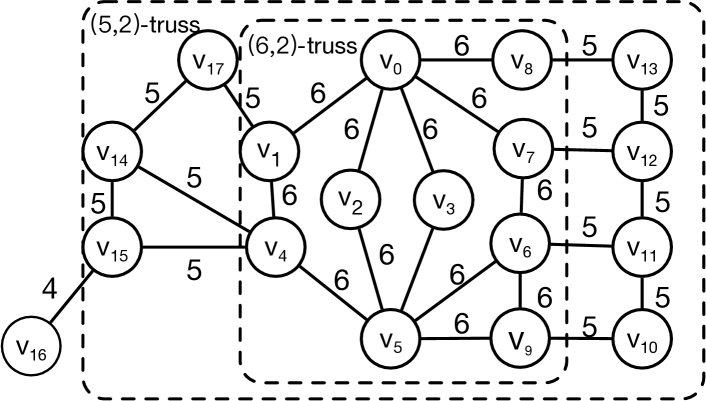
Example 2.1: Consider $G$ in Figure 2 and assume $\tau=2$ (in the following examples, we always assume $\tau=2$). For $v_{0}$, its 2-hop neighbors $N_{2}(v_{0},G)=\{v_{1},\dots,v_{8},v_{12},v_{13},v_{17}\}$. For $v_{1}$, its 2-hop neighbors $N_{2}(v_{1},G)=\{v_{0},v_{2},\dots,v_{5},v_{7},v_{8},v_{14},v_{15},v_{17}\}$. Therefore, $\Delta_{2}((v_{0},v_{1}),G)=N_{2}(v_{0},G)\cap N_{2}(v_{1},G)=\{v_{2},\dots v_{5},v_{7},v_{8},v_{17}\}$, ${\mathsf{sup}}_{2}((v_{0},v_{1}),G)=7$. ${\mathsf{sup}}_{2}(e,G)$ for each edge $e$ can be computed similarly and we can find that ${\mathsf{sup}}_{2}(e,G)\geq 2$. Thus, $G$ itself is a $(4,2)$-truss. Moreover, we can find that the subgraph $G^{\prime}$ induced by $\{v_{0},\dots,v_{15}\}$ is a $(5,2)$-truss as ${\mathsf{sup}}_{2}(e,G^{\prime})\geq 3$ for each edge $e$ in $G^{\prime}$ and no more edges can be added to $G^{\prime}$ to make it as a bigger $(5,2)$-truss. $\phi_{2}((v_{15},v_{16}),G)$ is 4 as $(v_{15},v_{16})$ is contained in the $(4,2)$-truss but not in the $(5,2)$-truss. The value of $\phi_{2}(e,G)$ is shown near each edge in Figure 2. The hierarchy structure of $G$ is clearly illustrated by the value of $\phi_{2}(e,G)$.

$\Box$

3 Theoretical Properties of $(k,\tau)$-truss

Although $\tau$-hop neighborhood is considered, $(k,\tau)$-truss still have the cohesiveness properties on degree and diameter:

Property 1: (Minimum Degree) Given a $(k,\tau)$-truss $G^{\prime}$ of $G$, for each vertex $v\in V(G^{\prime})$, $d_{\tau}(v,G^{\prime})\geq k-1$.

Proof.

For a vertex $v$, let $e=(u,v)$ be an edge incident to $v$ in $G^{\prime}$. Based on Definition 2, we have ${\mathsf{sup}}_{\tau}(e,G^{\prime})\geq k-2$. According to Definition 2, $v$ has at least $k-2$ $\tau$-hop neighbors in $\Delta_{\tau}(e,G)$. Moreover, $u$ is a 1-hop neighbor of $v$. Thus, $d_{\tau}(v,G^{\prime})\geq k-1$. ∎

Property 2: (Bounded Diameter) Given a $(k,\tau)$-truss $G^{\prime}$ of $G$, for each connected component $G^{\prime\prime}$ of $G^{\prime}$, the diameter of $G^{\prime\prime}$ $\omega(G^{\prime\prime})\leq\frac{2\tau(|V(G^{\prime\prime})|-1)}{k}$.

Proof.

Without loss of generality, let $p=(v_{1},v_{2},...,v_{d})$ be the shortest path in $G^{\prime\prime}$ with $l(p)=\omega(G^{\prime\prime})$. We use $V(p)$ to denote the set of vertices on $p$. For an edge $e_{i}=(v_{i},v_{i+1})$ on $p$, we use $\Gamma_{i}$ to denote the set of vertices in $\Delta_{\tau}(e_{i},G^{\prime\prime})\setminus V(p)$. According to Definition 2, it is clear that $|\Delta_{\tau}(e_{i},G^{\prime\prime})\cap V(p)|\leq 2\tau-2$. Since $\Gamma_{i}=\Delta_{\tau}(e_{i},G^{\prime\prime})\setminus(\Delta_{\tau}(e_{i},G^{\prime\prime})\cap V(p))$, $|\Gamma_{i}|=|\Delta_{\tau}(e_{i},G^{\prime\prime})|-|\Delta_{\tau}(e_{i},G^{\prime\prime})\cap V(p)|$. According to Definition 2, $|\Delta_{\tau}(e_{i},G^{\prime\prime})|\geq k-2$. Together with $|\Delta_{\tau}(e_{i},G^{\prime\prime})\cap V(p)|\leq 2\tau-2$, we have $|\Gamma_{i}|\geq k-2\tau$.

Meanwhile, for a vertex $w\in V(G^{\prime\prime})\setminus V(p)$, we have $|\{\Gamma_{i}:w\in\Gamma_{i},1\leq i\leq d-1\}|\leq 2\tau$. This can be proved by contraction. Assume that $|\{\Gamma_{i}:w\in\Gamma_{i},1\leq i\leq d-1\}|\geq 2\tau+1$, let $E_{\Gamma}$ be the set of edges on $p$ such that $w$ is a $\tau$-hop common neighbor. Based on the assumption, $|E_{\Gamma}|\geq 2\tau+1$. Let $e_{j}=(v_{j},v_{j+1})$ and $e_{k}=(v_{k},v_{k+1})$ be two edges in $E_{\Gamma}$ such that the edges on $p$ between $e_{j}$ and $e_{k}$ are maximum. We can derive that the length of the sub-path from $v_{j}$ to $v_{k+1}$ on $p$ is at least $2\tau+1$ due to $|E_{\Gamma}|\geq 2\tau+1$. On the other hand, since $w$ is a $\tau$-hop common neighbors of $e_{j}$ and $e_{k}$, there exists a path $p^{\prime}$ from $v_{j}$ to $v_{k+1}$ through $w$ with length less than $2\tau$. It contradicts with the assumption that $p$ is a shortest path from $v_{1}$ to $v_{d}$ as we can replace the sub-path from $v_{j}$ to $v_{k+1}$ on $p$ with $p^{\prime}$ to obtain a shorter path. Therefore, $|\{\Gamma_{i}:w\in\Gamma_{i},1\leq i\leq d-1\}|\leq 2\tau$. Based on this, we can derive that $|\Gamma_{1}\cup\Gamma_{2}...\cup\Gamma_{d-1}|\geq\frac{(d-1)(k-2\tau)}{2\tau}$. Since $V(G^{\prime\prime})=\Gamma_{1}\cup\Gamma_{2}...\cup\Gamma_{d-1}\cup V(p)$, $|V(G^{\prime\prime})|=|\Gamma_{1}\cup\Gamma_{2}...\cup\Gamma_{d-1}|+|V(p)|$, we can derive that $|V(G^{\prime\prime})|\geq\frac{(d-1)(k-2\tau)}{2\tau}+d$. As $\omega(G^{\prime\prime})=d-1$, $\omega(G^{\prime\prime})\leq\frac{2\tau(|V(G^{\prime\prime})|-1)}{k}$, the property holds. ∎

4 A Bottom-Up Decomposition Paradigm

In this section, we present a bottom-up decomposition algorithm for higher-order neighborhood truss decomposition, which is based on the following lemma:

Lemma 4.1: Given a graph $G$ and an integer $\tau$, a $(k+1,\tau)$-truss is contained by a $(k,\tau)$-truss.

Proof.

According to Definition 2, for each edge $e$ in a $(k+1,\tau)$-truss $G^{\prime}$, ${\mathsf{sup}}_{\tau}(e,G^{\prime})\geq k-1\geq k-2$. It is clear that $G^{\prime}$ is also a $(k,\tau)$-truss. ∎

Based on Lemma 4, for a given graph $G$, we can decompose $G$ in the increasing order of $k$. For a specific $k$, we compute the edges whose higher-order truss number is identical to $k$. As $(k+1,\tau)$-truss is contained in the $(k,\tau)$-truss, according to Definition 2, we can remove these edges from $G$ and get the $(k+1,\tau)$-truss. We continue the procedure and the higher-order truss number for each edge can be obtained when all the edges are removed. The pseudocode of the decomposition algorithm is shown in Algorithm 1

Algorithm. Following the above idea, the paradigm to conduct the higher-order truss decomposition, $\mathsf{HOTDecom}$, is shown in Algorithm 1. Given a graph $G$ and an integer $\tau$, it first computes the higher-order support for each edge in $G$ (line 1-2). Then, it determines the higher-order truss number for each edge by iteratively removing the edges until $G$ is empty (line 3-9). Specifically, it first assigns the value of the minimum higher-order support plus 2 among the edges in the remaining graph $G$ to $k$ (line 4). It means the remaining graph is at least a $(k,\tau)$-truss. Therefore, the higher-order truss number for the edges $e$ in the remaining graph with ${\mathsf{sup}}_{\tau}(e,G)\leq k-2$ is $k$ (line 6). After the higher-order truss number of $e$ is obtained, Algorithm 1 removes $e$ from $G$ (line 7). Due to the removal of $e$, the $\tau$-hop common neighbors of edges incident to vertices in $\{u\}\cup\{v\}\cup\Delta_{\tau}(e,G^{\prime})$ could be changed in $G$. Consequently, Algorithm 1 recomputes the higher-order support for these edges with ${\mathsf{sup}}_{\tau}(e^{\prime},G)>k-2$ (line 8-9). Algorithm 1 continues until $G$ is empty (line 3).

Algorithm 1 ${\mathsf{HOTDecom}}(G,\tau)$

1:  for each $e\in E(G)$ do

2:     compute ${\mathsf{sup}}_{\tau}(e,G)$;

3:  while $G\neq\emptyset$ do

4:     $k\leftarrow{\mathsf{min}}_{e\in E(G)}{\mathsf{sup}}_{\tau}(e,G)$ + 2;

5:     while $\exists~{}e=(u,v)\in E(G)$ with ${\mathsf{sup}}_{\tau}(e,G)\leq k-2$ do

6:        $\phi_{\tau}(e,G)\leftarrow k$;

7:        $G^{\prime}\leftarrow G$; $G\leftarrow G\setminus e$;

8:        for each $e^{\prime}=(u^{\prime},v^{\prime})\in E(G)$ with $u^{\prime},v^{\prime}\in\{u\}\cup\{v\}\cup\Delta_{\tau}(e,G^{\prime})$ with ${\mathsf{sup}}_{\tau}(e^{\prime},G)>k-2$ do

9:           compute ${\mathsf{sup}}_{\tau}(e^{\prime},G)$;

Figure 3: The procedure of $\mathsf{HOTDecom}$

Example 4.1: Reconsider the graph $G$ shown in Figure 2. Figure 3 shows the procedure of $\mathsf{HOTDecom}$ to conduct the decomposition. It first computes ${\mathsf{sup}}_{2}(e,G)$ for each edge, which is shown near each edge. Since the minimum value of ${\mathsf{sup}}_{2}(e,G)$ among all the edges in $G$ is 2, then $k$ is assigned as 4 and $\phi_{2}((v_{15},v_{16}),G)$ is 4. After that, $(v_{15},v_{16})$ is removed and $\mathsf{HOTDecom}$ needs to update the higher-order support of $(v_{14},v_{15})$. ${\mathsf{sup}}_{2}((v_{14},v_{15}),G)$ decreases from 5 to 4, following $(v_{4},v_{14})$ and $(v_{4},v_{15})$. $\mathsf{HOTDecom}$ continues the above procedure until all the edges are removed. When it finishes, the higher-order truss number for each edge is obtained. $\Box$

Theorem 4.1: Given a graph $G$ and an integer $\tau$, Algorithm 1 computes the higher-order truss number for each edge correctly.

Proof.

To show the correctness of Algorithm 1, we only need to prove that the value assigned to $\phi_{\tau}(e,G)$ in line 6 of Algorithm 1 is the correct higher-order truss number for every edge $e\in E(G)$.

Based on the procedure of Algorithm 1, for the first edge $e_{1}$ of $G$ processed in line 6, the value of $k$ is the correct higher-order truss number of $e_{1}$. This is because when $e_{1}$ is processed, ${\mathsf{sup}}_{\tau}(e,G)$ is correctly computed for every edge of $G$ in line 1-2 and the value of $k$ is the minimum value among all the computed ${\mathsf{sup}}_{\tau}(e,G)$ plus 2. Based on Definition 2, the graph $G$ itself is a $(k,\tau)$-truss. Therefore, the higher-order truss number of $e_{1}$ is correctly computed.

Next, we show that the higher-order truss number is also correctly computed for the following processed edges $e_{2},\dots,e_{m}$. We prove it by contradiction. Without loss of generality, let $e_{i}$ be the first edge assigned with wrong higher-order truss number, and the higher-order truss number assigned to $e_{i}$ by Algorithm 1 is $k_{1}$ while the correct higher-order truss number of $e_{i}$ is $k_{2}$. We first consider the case that $k_{1}<k_{2}$. As $e_{i}$ is the first edge assigned with wrong higher-order truss number and the correct higher-order truss number of $e_{i}$ is $k_{2}>k_{1}$, then, all the edges whose higher-order truss number is not less than $k_{2}$ have not been processed when processing $e_{i}$. According to Definition 2, these edges together with $e_{i}$ consist of a $(k_{2},\tau)$-truss and ${\mathsf{sup}}_{\tau}(e_{i},G)$ is at least not less than $k_{2}-2$. Meanwhile Algorithm 1 assigns $k_{1}$ to $\phi_{\tau}(e_{i},G)$ in line 6, it means ${\mathsf{sup}}_{\tau}(e_{i},G)$ is less than $k_{1}-2$ in line 5 before $e_{i}$ is processed in line 6. It leads to the contradiction against the assumption that $k_{1}<k_{2}$. Therefore, $k_{1}<k_{2}$ is impossible. Similarly, we can prove that $k_{1}>k_{2}$ is also impossible. Therefore, the higher-order truss number is also correctly computed for $e_{2},\dots,e_{m}$. Combining these two cases together, the theorem holds. ∎

Theorem 4.2: Given a graph $G$ and an integer $\tau$, the time complexity of Algorithm 1 is $O(m\cdot m_{\tau}\cdot(m_{\tau}+n_{\tau}))$, where $m_{\tau}$ and $n_{\tau}$ are the maximum numbers of edges and vertices within the $\tau$-hop neighborhood in the graph, respectively.

Proof.

In Algorithm 1, we first compute ${\mathsf{sup}}_{\tau}(e,G)$ for each edge in $G$ in line 1-2. To compute ${\mathsf{sup}}_{\tau}(e,G)$ for an edge $e=(u,v)$, we first retrieve $N_{\tau}(u,G)$ and $N_{\tau}(v,G)$ of $u$ and $v$ by breadth-first search, which costs $O(m_{\tau}+n_{\tau})$ time. Then, the computation of $\Delta_{\tau}(e,G)$ costs $O(n_{\tau})$ time. Therefore, the computation of line 1-2 can be finished in $O(m\cdot(m_{\tau}+n_{\tau}))$. For line 3-9, when an edge $e$ is removed in line 7, $O(m_{\tau})$ edges in its $\tau$-hop neighborhood need to update their higher-order edge support and each update consumes $O(m_{\tau}+n_{\tau})$ time. Therefore, the time for updating higher-order edge support in line 8-9 can be bounded by $O(m_{\tau}\cdot(m_{\tau}+n_{\tau}))$. In Algorithm 1, each edge is removed once in line 7 and line 4-5 can be finished in const time by using a bin array. As a result, the time complexity of line 3-9 can be bounded by $O(m\cdot m_{\tau}\cdot(m_{\tau}+n_{\tau}))$. Therefore, the overall time complexity of Algorithm 1 is $O(m\cdot m_{\tau}\cdot(m_{\tau}+n_{\tau}))$. ∎

5 An Improved Decomposition Algorithm

In this section, we aim to improve the performance of the bottom-up decomposition paradigm. According to Theorem 3, the most time-consuming part of Algorithm 1 is the higher-order support update in line 8-9. Compared with the time complexity of line 1-2, an additional term $m_{\tau}$ is introduced in that of line 3-9. When an edge $e$ is removed from $G$ in line 7, $\mathsf{HOTDecom}$ updates ${\mathsf{sup}}_{\tau}(e^{\prime},G)$ for all the edge $e^{\prime}$ incident to vertices in $\{u\}\cup\{v\}\cup\Delta_{\tau}(e,G^{\prime})$ in line 8-9 immediately. The immediate update strategy adopted by $\mathsf{HOTDecom}$ leads to the term $m_{\tau}$ in Theorem 3, which makes it prohibitively costly.

To address the performance issue in $\mathsf{HOTDecom}$, we explore three optimization strategies, namely delayed update strategy, early pruning strategy, and unchanged support detection strategy to avoid unnecessary higher-order support update. In this section, we first show these three proposed strategies. Then, we present our improved algorithm for the higher-order truss decomposition.

5.1 A Delayed Update Strategy

Since the immediate update strategy leads to the term $m_{\tau}$ in the time complexity of $\mathsf{HOTDecom}$, our first idea is to explore the opportunities to delay the higher-order support update until necessary. To achieve this goal, we first define:

Definition 5.1: (Truss Number Bounded Edge Set) Given a graph $G$, an integer $\tau$, and a condition $f(\phi)$, the truss number bounded edge set, denoted by $\Phi_{\tau,f(\phi)}(G)$, is the set of edges whose higher-order truss number $\phi_{\tau}(e,G)$ satisfies $f(\phi)$. $\Box$

Revisiting Algorithm 1, the key point to guarantee the correctness of the $\mathsf{HOTDecom}$ is that the value of ${\mathsf{sup}}_{\tau}(e,G)$ for an edge $e\in\Phi_{\tau,\phi=k}(G)$ must be not greater than $k-2$ when handling a specific $k$ in line 5-6. Following this, $\mathsf{HOTDecom}$ updates ${\mathsf{sup}}_{\tau}(e^{\prime},G)$ for the edges incident to vertices in $\{u\}\cup\{v\}\cup\Delta_{\tau}(e,G^{\prime})$ to keep the invariant. On the other hand, according to Definition 2, when handling a specific $k$, for an edge $e^{\prime\prime}\in\Phi_{\tau,\phi>k}(G)$, it is not necessary to update the value of ${\mathsf{sup}}_{\tau}(e^{\prime\prime},G)$ immediately based on the following two reasons: (1) for the edge $e\in\Phi_{\tau,\phi=k}(G)$, the value of ${\mathsf{sup}}_{\tau}(e^{\prime\prime},G)$ does not affect the correctness of computing $\phi_{\tau}(e,G)$ in Algorithm 1 as ${\mathsf{sup}}_{\tau}(e^{\prime\prime},G)\geq\phi_{\tau}(e^{\prime\prime},G)-2>k-2$. (2) For the edge $e^{\prime\prime}$ itself, we can delay the computation of ${\mathsf{sup}}_{\tau}(e^{\prime\prime},G)$ until handling $k$ whose value is identical to $\phi_{\tau}(e^{\prime\prime},G)$ as $\phi_{\tau}(e^{\prime\prime},G)$ is determined only by $\Phi_{\tau,\phi\geq k}$.

Following this idea, assume that we have already known the higher-order truss number of edges in prior, then, when an edge $e$ is removed in line 7 of Algorithm 1, instead of updating ${\mathsf{sup}}_{\tau}(e^{\prime},G)$ for the edge $e^{\prime}$ incident to vertices in $\{u\}\cup\{v\}\cup\Delta_{\tau}(e,G^{\prime})$, we only need to update ${\mathsf{sup}}_{\tau}(e^{\prime},G)$ for edges with $\phi_{\tau}(e^{\prime})=k$. With this delayed update strategy, we can significantly reduce the number of edges updating their values of ${\mathsf{sup}}_{\tau}(e^{\prime},G)$ in line 9, which improves the performance of $\mathsf{HOTDecom}$ consequently.

Lower bound of $\phi_{\tau}(e,G)$. However, it is intractable to obtain the higher-order truss number directly before the decomposition as it is our goal. Despite the intractability, for an edge $e^{\prime}$, if we can obtain a lower bound $\underline{\phi}_{\tau}(e^{\prime},G)$ of its higher-order truss number rather than the exact value, when handling a specific $k$, we only update ${\mathsf{sup}}_{\tau}(e^{\prime},G)$ for edges with $\underline{\phi}_{\tau}(e^{\prime},G)\leq k$, the above inference still establishes. Therefore, the remaining problem is how to obtain a tight lower bound for an edge efficiently. To achieve this goal, we have the following lemma:

Lemma 5.1: Given a graph $G$ and an integer $\tau$, let $G^{\prime}$ be a subgraph of $G$, for any edge $e\in E(G^{\prime})$, $\phi_{\tau}(e,G)\geq\phi_{\tau}(e,G^{\prime})$.

Proof.

This lemma can be proved directly based on Definition 2. ∎

According to Lemma 5.1, for an edge in a graph $G$, the higher-order truss number of the edge in any subgraph of $G$ is a lower-bound of the higher-order truss number of the edge in $G$. Moreover, we have the following lemma:

Lemma 5.2: Given a graph $G$, for a subgraph $G^{\prime}$ in $G$, if the diameter $\omega(G^{\prime})\leq\tau$, then $G^{\prime}$ is a $(|V(G^{\prime})|,\tau)$-truss.

Proof.

Since the diameter $\omega(G^{\prime})\leq\tau$, each vertex in $G^{\prime}$ is $\tau$-hop reachable with each other. It means that for an edge $e=(u,v)$ in $G^{\prime}$, the $\tau$-hop common neighbors of $e$ in $G^{\prime}$ are all other vertices in $G^{\prime}$ except $u$ and $v$. Therefore, we can drive that ${\mathsf{sup}}_{\tau}(e,G^{\prime})=|V(G^{\prime})|-2$ for all the edges in $G^{\prime}$. According to Definition 2, $G^{\prime}$ is a $(|V(G^{\prime})|,\tau)$-truss. The lemma holds. ∎

According to Lemma 5.1 and Lemma 5.1, for a graph $G$ and an integer $\tau$, if we have a subgraph $G^{\prime}$ of $G$ such that $\omega(G^{\prime})\leq\tau$, then, for any edge $e\in E(G^{\prime})$, we have $\phi_{\tau}(e,G)\geq|V(G^{\prime})|$. Based on this, we define:

Definition 5.2: (Vertex Centric $\tau$-Diameter Subgraph) Given a graph $G$ and an integer $\tau$, for a vertex $v\in V(G)$, the vertex centric $\tau$-diameter subgraph of $v$, denoted by $\Omega(v)$, is the subgraph of $G$ induced by the set of vertices in $\{v\}\cup\{w|w\rightarrow_{\lfloor\frac{\tau}{2}\rfloor}v\}$. $\Box$

Lemma 5.3: Given a vertex $v$ in a graph $G$ and an integer $\tau$, for an edge $e=(u,v)\in E(G)$, $\phi_{\tau}(e,G)\geq|V(\Omega(v))|$.

Proof.

We consider two cases: (1) $\tau$ is even. Based on Definition 5.1, $\omega(\Omega(v))\leq\tau$. According to Lemma 5.1, $\Omega(v)$ is a $(|V(\Omega(v)|,\tau)$-truss. Since $\Omega(v)$ is a subgraph of $G$, according to Lemma 5.1, $\phi_{\tau}(e,G)\geq|V(\Omega(v))|$. (2) $\tau$ is odd. Based on Definition 5.1, $\omega(\Omega(v))\leq\tau-1$. According to Lemma 5.1, $\Omega(v)$ is a $(|V(\Omega(v)|,\tau-1)$-truss. As $\Omega(v)$ is a subgraph of $G$, according to Lemma 5.1, $\phi_{\tau-1}(e,G)\geq|V(\Omega(v))|$. Following Definition 2, $\phi_{\tau}(e,G)\geq\phi_{\tau-1}(e,G)$. Thus, $\phi_{\tau}(e,G)\geq|V(\Omega(v))|$. Combining the above two cases, the lemma holds. ∎

Following Lemma 5.1, for an edge $e=(u,v)\in E(G)$, we can derive that $\phi_{\tau}(e,G)\geq|V(\Omega(u))|$ as well. Moreover, we can also derive that:

Lemma 5.4: Given a graph $G$ and an integer $\tau$, for an edge $e=(u,v)\in E(G)$, $\phi_{\tau}(e,G)\geq{\mathsf{max}}\{|V(\Omega(w))|\}$, where $w\in\Delta_{\lfloor\frac{\tau}{2}\rfloor}(e,G)$.

Proof.

This lemma can be proved similarly as Lemma 5.1. ∎

According to Lemma 5.1 and Lemma 5.1, for an edge $e=(u,v)$, a lower bound of $e$ is ${\mathsf{max}}\{|V(\Omega(u))|$, $|V(\Omega(v))|,|V(\Omega(w))|\}$, where $w\in\Delta_{\lfloor\frac{\tau}{2}\rfloor}(e,G)$. However, in this case, if $\tau$ is odd, the value of $\underline{\phi}_{\tau}(e,G)$ is identical to that of $\underline{\phi}_{\tau-1}(e,G)$. To address this problem, we define:

Definition 5.3: (Edge Centric $\tau$-Diameter Subgraph) Given a graph $G$ and an odd integer $\tau$, for an edge $e=(u,v)\in E(G)$, the edge centric $\tau$-diameter subgraph of $e$, denoted by $\Omega(e)$, is the subgraph of $G$ induced by the set of vertices in $\{u\}\cup\{v\}\cup\{w|w\rightarrow_{\lfloor\frac{\tau}{2}\rfloor}u\vee w\rightarrow_{\lfloor\frac{\tau}{2}\rfloor}v\}$. $\Box$

Lemma 5.5: Given an edge $e$ in a graph $G$ and an odd integer $\tau$, $\phi_{\tau}(e,G)\geq|V(\Omega(e))|$.

Proof.

The lemma can be prove similarly as Lemma 5.1. ∎

Therefore, our lower bound is defined as follows:

Definition 5.4: (Lower Bound $\underline{\phi}_{\tau}(e,G)$ ) Given a graph $G$ and an integer $\tau$, for an edge $e=(u,v)\in E(G)$, $\underline{\phi}_{\tau}(e,G)=$

$$\begin{cases}~{}{\mathsf{max}}\{|V(\Omega(u))|,|V(\Omega(v))|,|V(\Omega(w))|\},&\tau~{}is~{}even\\ ~{}{\mathsf{max}}\{|V(\Omega(e))|,|V(\Omega(w))|\},&\tau~{}is~{}odd,\\ \end{cases}$$

where $w\in\Delta_{\lfloor\frac{\tau}{2}\rfloor}(e,G)$. $\Box$

(a) $\tau$ is even

(b) $\tau$ is odd

Figure 4: $\underline{\phi}_{\tau}(e,G)$ for an edge $e=(u,v)$

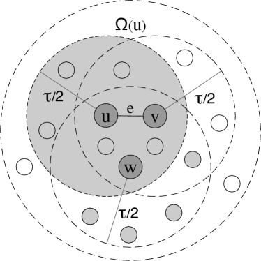
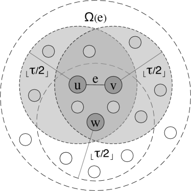
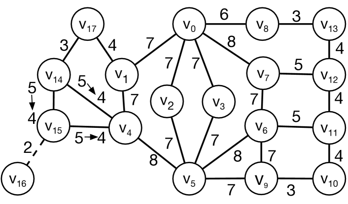
Example 5.1: Figure 4 illustrates the idea of $\underline{\phi}_{\tau}(e,G)$ for an edge $e=(u,v)$. In Figure 4 (a), the shadowed dashed circle represents the vertex centric $\tau$-diameter subgraph $\Omega(u)$. In Figure 4 (b), the shadowed part represents the edge centric $\tau$-diameter subgraph $\Omega(e)$. When $\tau$ is even, we choose ${\mathsf{max}}\{|V(\Omega(u))|$,$|V(\Omega(v))|$,$|V(\Omega(w))|\}$ as $\underline{\phi}_{\tau}(e,G)$. When $\tau$ is odd, we choose ${\mathsf{max}}\{|V(\Omega(e))|,|V(\Omega(w))|\}$ as $\underline{\phi}_{\tau}(e,G)$. For a concrete example, consider the graph $G$ shown in Figure 2, take the edge $(v_{0},v_{1})$ as an example, $\tau=2$, since $\tau$ is even, we just need to consider $\Omega(v_{0})=\{v_{0},v_{1},v_{2},v_{3},v_{7},v_{8}\}$, $\Omega(v_{1})=\{v_{0},v_{1},v_{4},v_{17}\}$. Therefore, $\underline{\phi}_{2}((v_{0},v_{1}),G)={\mathsf{max}}\{|\Omega(v_{0})|,|\Omega(v_{1})|\}=6$. $\Box$

5.2 An Early Pruning Strategy

With the lower bound, we can delay the computation of higher-order support when necessary, which consequently reduces the number of higher-order support update in line 8-9 of Algorithm 1. On the other hand, when handling a specific $k$ during decomposition, if we have some lightweight methods that can determine the higher-order truss number of an edge $e$ cannot be larger than $k$, then we can directly obtain $\phi_{\tau}(e,G)=k$, which means we can correctly obtain the higher-order truss number of $e$ without the computation of its higher-order support. As a result, we can still reduce the number of higher-order support update and improve the performance of $\mathsf{HOTDecom}$. Following this idea, we have:

Lemma 5.6: Given a graph $G$, two integers $k$ and $\tau$, for an edge $e=(u,v)\in V(G)$, if $d_{\tau}(u,G)\leq k-1\vee d_{\tau}(v,G)\leq k-1$, $\phi_{\tau}(e,G)\leq k$.

Proof.

According to Property 3, if $d_{\tau}(u,G)\leq k-1$ (resp. $d_{\tau}(v,G)\leq k-1)$, $u$ (resp. $v$) is not contained in a $(k+1,\tau)$-truss. Thus, $e$ is not contained in a $(k+1,\tau)$-truss. Based on Definition 2, $\phi_{\tau}(e,G)\leq k$. ∎

With Lemma 5.2, when handling a specific $k$, we can prune an edge by computing the $\tau$-hop degree of its two incident vertices. Moreover, if we have computed $d_{\tau}(v,G)$ for a vertex $v$ and the value of $d_{\tau}(v,G)$ is not greater than $k-1$, then all the edges incident to $v$ can be pruned. In other words, by computing the $\tau$-hop degree of a single vertex, we can reduce the computation of higher-order support for multiple edges, which achieves the goal of early pruning.

5.3 An Unchanged Support Detection Strategy

In addition to the above discussed optimization strategies, here, we aim to explore the edges whose higher-order support unchanged after the removal of an edge to avoid the update. When an edge $e=(u,v)$ is removed , we have:

Lemma 5.7: Given an edge $e=(u,v)$ in a graph $G$, let $G^{\prime}$ be the graph after the removal of $e$, for an edge $e^{\prime}=(u^{\prime},v^{\prime})$ in $G^{\prime}$ where $u^{\prime},v^{\prime}\in\Delta_{\tau}(e,G)$, if the distance between $u$ (resp. $v$) to $u^{\prime}$ (resp. $v^{\prime}$) in $G$ and $G^{\prime}$ keep the same, then, ${\mathsf{sup}}_{\tau}(e^{\prime},G)={\mathsf{sup}}_{\tau}(e^{\prime},G^{\prime})$.

Proof.

According to Definition 2, we can prove the lemma if we can prove that $N_{\tau}(u^{\prime},G)=N_{\tau}(u^{\prime},G^{\prime})$ and $N_{\tau}(v^{\prime},G)=N_{\tau}(v^{\prime},G^{\prime})$. Therefore, we first prove $N_{\tau}(u^{\prime},G)=N_{\tau}(u^{\prime},G^{\prime})$. It can be proved by contradiction. Assume that $N_{\tau}(u^{\prime},G)$ and $N_{\tau}(u^{\prime},G^{\prime})$ are different due to the removal of $e^{\prime}$. Since the removal of an edge only leads to the reduction of $\tau$-hop reachable vertices from a specific vertex, we can derive that $N_{\tau}(u^{\prime},G^{\prime})\subseteq N_{\tau}(u^{\prime},G)$. Without lose of generality, let $w$ be a vertex in $N_{\tau}(u^{\prime},G)\setminus N_{\tau}(u^{\prime},G^{\prime})$. Then, we can derive $u^{\prime}\rightarrow_{\tau}w$ in $G$ but $u^{\prime}\nrightarrow_{\tau}w$ in $G^{\prime}$ according to Definition 2. Therefore, the shortest path from $u^{\prime}$ to $w$ must pass through $(u,v)$ in $G$. Let the shortest path from $u^{\prime}$ to $w$ be $p=(u^{\prime},\dots,u,v,\dots,w)$. Since the shortest path from $u^{\prime}$ to $w$ passes through $(u,v)$, we can derive that the shortest path from $u^{\prime}$ to $v$ is the sub-path $p^{\prime}=(u^{\prime},\dots,u,v)$ of $p$ and $l(p^{\prime})<l(p^{\prime\prime})$, where $p^{\prime\prime}$ is other arbitrary path from $u^{\prime}$ to $v$ not passing through $(u,v)$ in $G$. Therefore, after the removal of $e$, the distance between $u^{\prime}$ and $v$ must be larger than $l(p^{\prime})$ in $G^{\prime}$, which contradicts with the fact that distance between $u^{\prime}$ and $v$ in $G$ and $G^{\prime}$ are the same. Therefore, $N_{\tau}(u^{\prime},G)=N_{\tau}(u^{\prime},G^{\prime})$. Similarly, we can prove $N_{\tau}(v^{\prime},G)=N_{\tau}(v^{\prime},G^{\prime})$. Therefore, ${\mathsf{sup}}_{\tau}(e^{\prime},G)={\mathsf{sup}}_{\tau}(e^{\prime},G^{\prime})$. ∎

According to Lemma 5.3, for an edge $(u,v)$ in $G$, we can maintain the distance between $u$ (resp. $v$) and the vertices in $\Delta_{\tau}(e,G)$ before and after the removal of $(u,v)$. For those vertices $V^{\prime}\subseteq\Delta_{\tau}(e,G)$ such that the distance between them and $u$ (resp. $v$) keep the same, we can guarantee that the higher-order support of the edge $e^{\prime}$ connecting any two vertices in $V^{\prime}$ is unchanged after the removal of $(u,v)$. Compared with updating the higher-order support for these edges $e^{\prime}$ directly, the above distance can be obtained by just two BFS traversals starting from $u$ and $v$, respectively, which means we can further reduce the number of edges that need to update their higher-order support with little cost.

5.4 The Improved Algorithm

Algorithm 2 ${\mathsf{HOTDecom^{+}}}(G,\tau)$

1:  for each $e\in E(G)$ do

2:   compute $\underline{\phi}_{\tau}(e,G)$;

3:  $k\leftarrow min_{e\in E(G)}(\underline{\phi}_{\tau}(e,G))$;

4:  while $G\neq\emptyset$ do

5:   for each $e\in E(G)$ with $\underline{\phi}_{\tau}(e,G)=k$ do

6:     compute ${\mathsf{sup}}_{\tau}(e,G)$;

7:   while $\exists~{}e=(u,v)\in E(G)$ with ${\mathsf{sup}}_{\tau}(e,G)\leq k-2$ do

8:     $\phi_{\tau}(e,G)\leftarrow k$; $G^{\prime}\leftarrow G$; $G\leftarrow G\setminus e$;

9:     for each $e^{\prime}=(u^{\prime},v^{\prime})\in E(G)$ with $u^{\prime},v^{\prime}\in\{u\}\cup\{v\}\cup\Delta_{\tau}(e,G^{\prime})$ do

10:      if $\underline{\phi}_{\tau}(e^{\prime},G^{\prime})>k$  then

11:        continue;                // delayed update

12:      if  ${\mathsf{pruneVertex}}(G,u^{\prime},k)$ or ${\mathsf{pruneVertex}}(G,v^{\prime},k)$ then

13:        continue;                 // early pruning

14:      compute ${\mathsf{dis}}_{G}(u,w)$, ${\mathsf{dis}}_{G^{\prime}}(u,w)$, ${\mathsf{dis}}_{G}(v,w)$, ${\mathsf{dis}}_{G^{\prime}}(v,w)$ with $w\in\Delta_{\tau}(e,G^{\prime})$;

15:      if ${\mathsf{dis}}_{G^{\prime}}(u,u^{\prime})$ = ${\mathsf{dis}}_{G}(u,u^{\prime})\wedge{\mathsf{dis}}_{G^{\prime}}(u,v^{\prime})$ = ${\mathsf{dis}}_{G}(u,v^{\prime})\wedge{\mathsf{dis}}_{G^{\prime}}(v,u^{\prime})$=${\mathsf{dis}}_{G}(v,u^{\prime})\wedge{\mathsf{dis}}_{G^{\prime}}(v,v^{\prime})$=${\mathsf{dis}}_{G}(v,v^{\prime})$ then

16:        continue;                 // unchanged support detection

17:      if ${\mathsf{sup}}_{\tau}(e^{\prime},G^{\prime})>k-2$ then

18:        compute ${\mathsf{sup}}_{\tau}(e^{\prime},G)$;

19:   $k\leftarrow k+1$;

Algorithm 3 $\mathsf{pruneVertex}$ ($G,v,k$)

1:  $\mathcal{S}\leftarrow\emptyset$; compute $d_{\tau}(v,G)$;

2:  if $d_{\tau}(v,G)\leq k-1$ then

3:   $\mathcal{S}.{\mathsf{put}}(v)$;

4:   while $\mathcal{S}\neq\emptyset$ do

5:     $u\leftarrow\mathcal{S}.{\mathsf{get}}()$;

6:     for each $e=(u,w)\in E(G)$ with $w\in N_{1}(u,G)$ do

7:      $\phi_{\tau}(e,G)\leftarrow k$;

8:     $G^{\prime}\leftarrow G$; $G\leftarrow G\setminus u$; $\mathcal{N}\leftarrow N_{\tau}(u,G^{\prime})$;

9:     for each $w\in\mathcal{N}$ do

10:      if $d_{\tau}(w,G)\leq k-1$ then $\mathcal{S}.{\mathsf{put}}(w)$; $\mathcal{N}\leftarrow\mathcal{N}\setminus w$;

11:     for each $e^{\prime\prime}=(x,y)\in E(G)$ with $x,y\in\mathcal{N}$  do

12:      if $\underline{\phi}_{\tau}(e^{\prime\prime},G^{\prime})\leq k$ then compute ${\mathsf{sup}}_{\tau}(e^{\prime\prime},G)$;

13:   return true;

14:  else

15:   return false;

With the delayed update strategy, early pruning strategy and unchanged support detection strategy, we are ready to present our improved algorithm $\mathsf{HOTDecom^{+}}$, which is shown in Algorithm 2.

Algorithm. Algorithm 2 shares a similar framework as Algorithm 1. It first computes the lower bound $\underline{\phi}_{\tau}(e,G)$ for each edge (line 1-2). Then, it decomposes the graph in the increasing order of $k$. It first initializes $k$ as the minimum value of $\underline{\phi}_{\tau}(e,G)$ of all edges in $G$. For a specific $k$, Algorithm 2 first computes ${\mathsf{sup}}_{\tau}(e,G)$ for each edge with $\underline{\phi}_{\tau}(e,G)=k$ (line 5-6). Then, for the edge with ${\mathsf{sup}}_{\tau}(e,G)\leq k-2$, it assigns the higher-order truss number to $e$ and removes $e$ from $G$ similarly as Algorithm 1 (line 7-8). After removing $e$, Algorithm 2 updates the higher-order support for the edges $e^{\prime}=(u^{\prime},v^{\prime})$ incident to vertices in $\{u\}\cup\{v\}\cup\Delta_{\tau}(e,G^{\prime})$. It first checks whether $\underline{\phi}_{\tau}(e^{\prime},G^{\prime})>k$. If it is true, Algorithm 2 delays the computation of ${\mathsf{sup}}_{\tau}(e^{\prime},G)$ (line 10-11). Otherwise, Algorithm 2 checks whether vertex $u^{\prime}$ or $v^{\prime}$ can be early pruned by $\mathsf{pruneVertex}$ (line 12-13). If these two vertices can not be pruned, it further checks whether the distance between $u$ (resp. $v$) and $u^{\prime}$ (resp. $v^{\prime}$) is changed (line 15-16). If the distance is changed and ${\mathsf{sup}}_{\tau}(e^{\prime},G^{\prime})>k-2$ , Algorithm 2 recomputes ${\mathsf{sup}}_{\tau}(e^{\prime},G)$ (line 18). Algorithm 2 continues the above procedure until $G$ is empty (line 4).

$\mathsf{pruneVertex}$ prunes the vertices based on Lemma 5.2. It uses a set $\mathcal{S}$ to record the vertices that can be pruned. For a vertex $v$, it first computes $d_{\tau}(v,G)$ (line 1). If $d_{\tau}(v,G)$ is not greater than $k-1$, $v$ is put in $\mathcal{S}$ (line 2-3). Then, it iteratively gets vertex $u$ from $\mathcal{S}$ until $\mathcal{S}$ is empty. For $u$, since $u$ can be pruned from $G$, which means the higher-order truss number for edges $e$ incident to $u$ is $k$, it assigns $k$ to $\phi_{\tau}(e,G)$ and removes the vertex from $G$ (line 6-8). Due to the removal of $u$, the $\tau$-hop degree for the vertices in $N_{\tau}(u,G^{\prime})$ may be changed. Therefore, it further checks the $\tau$-hop degree of these vertices. If these vertices can be pruned, then they are put in $\mathcal{S}$ and removed from $\mathcal{N}$ (line 8-10). For the edges whose two incident vertices are in the $\mathcal{N}$, it recomputes their higher-order edge support if $\underline{\phi}_{\tau}(e^{\prime\prime},G^{\prime})\leq k$ (line 11-12). If the procedure prunes any vertices, it returns true (line 13). Otherwise, it returns false (line 15).

Figure 5: The procedure of ${\mathsf{HOTDecom^{+}}}$

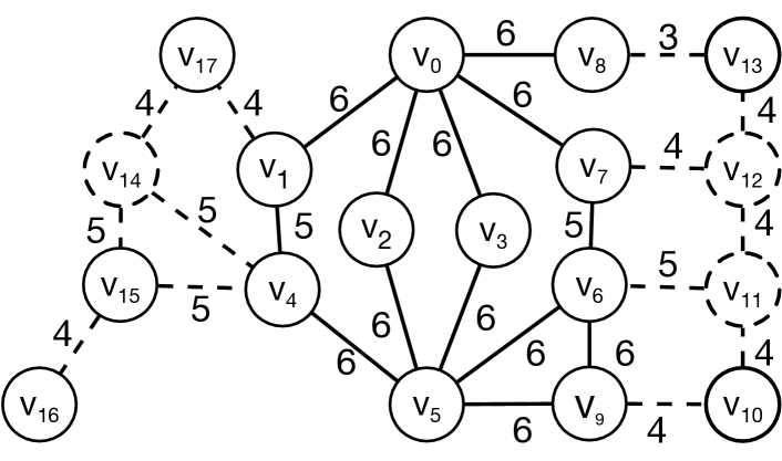
Example 5.2: Reconsider the graph $G$ shown in Figure 2. Figure 5 shows the procedure of $\mathsf{HOTDecom^{+}}$. It first computes lower bound $\underline{\phi}_{2}(e,G)$ for each edge. $\underline{\phi}_{2}(e,G)$ is shown near each edge in Figure 2. After that, it starts the decomposition with $k=3$. Since $\underline{\phi}_{2}((v_{8},v_{13}),G)=3$, it computes ${\mathsf{sup}}_{2}((v_{8},v_{13}),G)=3>k-2$. Then, $k$ becomes 4 and it computes ${\mathsf{sup}}_{2}(e,G)$ for edges with $\underline{\phi}_{2}(e,G)=4$. It gets ${\mathsf{sup}}_{2}((v_{15},v_{16}),G)=2$, ${\mathsf{sup}}_{2}((v_{14},v_{15}),G)=5$, $\dots$. Then, it removes $(v_{15},v_{16})$. Due to the removal of $(v_{15},v_{16})$ , ${\mathsf{sup}}_{2}((v_{14},v_{15}),G)$ is updated from 5 to 4, since $\underline{\phi}_{2}((v_{4},v_{14}),G)=5$$>$$4$ and $\underline{\phi}_{2}((v_{4}$,$v_{15})$,$G)=5$$>$$4$, it does not update their higher-order support. Then, $k$ becomes 5, since ${\mathsf{sup}}_{2}((v_{14},v_{17}),G)=3\leq 5-2$, $(v_{14},v_{17})$ is removed. Here, although $v_{1},v_{4}\in\Delta_{2}((v_{14},v_{17}),G)$, it does not update the higher-order support of $(v_{1},v_{4})$, $(v_{1},v_{17})$ and $(v_{4},v_{17})$ since the distance between $v_{1}$ (resp. $v_{4}$) and $v_{14}$ (resp. $v_{17}$) is unchanged after the removal of $(v_{14},v_{17})$. Meanwhile, due to the removal of $(v_{14},v_{17})$, $d_{2}(v_{14},G)$ is updated from 5 to 4, hence $v_{14}$ and its incident edges are removed directly. $(v_{4},v_{15})$ is removed following $v_{14}$. Here, although $v_{4},v_{5}\in\Delta_{2}((v_{4},v_{14})\cap\Delta_{2}((v_{4},v_{15})$, it does not update the support of $(v_{4},v_{5})$ as $\underline{\phi}_{2}((v_{4},v_{5}),G)>5$. Similarly, edges and vertices are removed until $G$ is empty. As shown in this example, many higher-order support updates are avoided compared with $\mathsf{HOTDecom}$ shown in Example 3. $\Box$

Theorem 5.1: Given a graph $G$ and an integer $\tau$, Algorithm 2 computes the higher-order truss number for each edge correctly.

Proof.

Following Theorem 3, we only need to show that the reduced higher-order updates caused by line 11-16 of Algorithm 2 do not affect the correctness of the algorithm. This can be guaranteed by Lemma 5.1, Lemma 5.1, Lemma 5.2, and Lemma 5.3. ∎

Theorem 5.2: The time complexity of Algorithm 2 is $O(m\cdot m_{\tau}\cdot(m_{\tau}+n_{\tau}))$.

Although $\mathsf{HOTDecom^{+}}$ shares the same worst case time complexity as $\mathsf{HOTDecom}$, lots of higher-order edge support updates can be reduced in practice as verified in our experiments, which makes $\mathsf{HOTDecom^{+}}$ significantly outperforms $\mathsf{HOTDecom}$.

6 Top-$r$ Higher-Order Trusses Computation

In the above section, we investigate the higher-order truss decomposition problem that the $(k,\tau)$-trusses with all possible $k$ values are computed. However, in some applications, users are only interested in the $(k,\tau)$-truss with a large $k$ value since the $(k,\tau)$-truss with large $k$ value is generally more cohesive and represents the core part of the graph Lee et al. (2010); Yuan et al. (2016b). Certainly, we can use $\mathsf{HOTDecom^{+}}$ directly to address this problem. Nevertheless, as this approach adopts the bottom-up decomposition paradigm, the $(k,\tau)$-trusses with small $k$ values have to be computed, which leads to lots of unnecessary computation. To address this problem, in this section, we propose a new approach tailored for the top $r$ $(k,\tau)$-trusses computation problem. Formally, given a graph $G$ and two integers $r$ and $\tau$, the top $r$ $(k,\tau)$-trusses computation problem returns the $(k,\tau)$-trusses with $k$ values in the range of $(k_{\mathsf{max}}-r,k_{{\mathsf{max}}}]$, where $k_{\mathsf{max}}$ is the maximum value of $k$ such that there is a non-empty $(k,\tau)$-truss regarding the corresponding $k$ value in the graph.

An upper-bound integrated approach. To conduct the top $r$ $(k,\tau)$-trusses computation, suppose that we have known the $\phi_{\tau}(e,G)$ for each edge $e$ in $G$ in prior, we can take the edges $\Phi_{\tau,\phi>k_{\mathsf{max}}-r}$ as the input of $\mathsf{HOTDecom^{+}}$ and conduct the decomposition starting from $k_{{\mathsf{max}}}-r+1$ to compute the result. In this way, the unnecessary computation involved in $\mathsf{HOTDecom^{+}}$ can be totally avoided. However, this approach has to know $\phi_{\tau}(e,G)$ for each edge $e$ in $G$ in prior, which is intractable. On the other hand, if we can obtain an upper bound $\overline{\phi}_{\tau}(e,G)$ for each edge $e$ in $G$, we can take the edges with $\overline{\phi}_{\tau}(e,G)>k_{{\mathsf{max}}}-r$ as the input of $\mathsf{HOTDecom^{+}}$ and obtain the correct answer for the similar reason as $\mathsf{HOTDecom^{+}}$. Following this idea, we propose an upper bound integrated approach to realize the top $r$ $(k,\tau)$-trusses computation. We first present the upper bound of $\phi_{\tau}(e,G)$.

Upper bound of $\phi_{\tau}(e,G)$. For an edge $e$ in a given graph $G$, a direct upper bound of $\phi_{\tau}(e,G)$ is ${\mathsf{sup}}_{\tau}(e,G)$. However, this bound is too loose. To obtain a tight upper bound, we define:

Definition 6.1: (Support-Vertex Bounded Subgraph) Given a graph $G$ and an integer $\tau$, for an edge $e=(u,v)\in E(G)$, let $G^{\prime}$ be the subgraph induced by $\{u\}\cup\{v\}\cup\{\Delta_{\tau}(e,G)\}$, the support-vertex bounded subgraph of $e$, denoted by $\Lambda(e)$, is a connected subgraph $G^{\prime\prime}$ of $G^{\prime}$ such that (1) $e\in E(G^{\prime\prime})$ (2) for each edge $e\in E(G^{\prime\prime})$, ${\mathsf{sup}}_{\tau}(e,G)\geq|V(G^{\prime\prime})|-2$ (3) $|V(G^{\prime\prime})|$ is maximal. $\Box$

Lemma 6.1: Given a graph $G$ and an integer $\tau$, for an edge $e=(u,v)$, $\phi_{\tau}(e,G)\leq|V(\Lambda(e))|$.

Proof.

We can prove it by contraction. Assume that there exists an edge $e^{\prime}=(u^{\prime},v^{\prime})$ such that $\phi_{\tau}(e^{\prime},G)>|V(\Lambda(e^{\prime}))|$. Based on Definition 2, let $\mathbb{G}$ be the subgraph of $G^{\prime\prime}$ induced by $\{u^{\prime}\}\cup\{v^{\prime}\}\cup\{\Delta_{\tau}(e^{\prime},G)\}$, where $G^{\prime\prime}$ is the $(\phi_{\tau}(e^{\prime},G),\tau)$-truss in $G$ containing $e^{\prime}$. Based on Definition 2, for each edge $e^{\prime\prime}\in E(\mathbb{G})$, ${\mathsf{sup}}_{\tau}(e^{\prime\prime},G^{\prime\prime})\geq\phi_{\tau}(e^{\prime\prime},G)-2$. Moreover, ${\mathsf{sup}}_{\tau}(e^{\prime\prime},G)\geq{\mathsf{sup}}_{\tau}(e^{\prime\prime},G^{\prime\prime})$. Therefore, ${\mathsf{sup}}_{\tau}(e^{\prime\prime},G)\geq\phi_{\tau}(e^{\prime\prime},G)-2\geq\phi_{\tau}(e^{\prime},G)-2>|V(\Lambda(e^{\prime}))|-2$. Meanwhile, $|V(\mathbb{G})|\geq\phi_{\tau}(e^{\prime},G)>|V(\Lambda(e^{\prime}))|$. It means $\mathbb{G}$ satisfies condition (1) and (2) of Definition 6 but the number of vertices is bigger than $|V(\Lambda(e^{\prime}))|$, which contracts with condition (3) of Definition 6. Thus, the lemma holds. ∎

Definition 6.2: (Upper Bound $\overline{\phi}_{\tau}(e,G)$) Given a graph $G$ and an integer $\tau$, for an edge $e\in E(G)$, $\overline{\phi}_{\tau}(e,G)=|V(\Lambda(e))|$. $\Box$

Algorithm 4 ${\mathsf{HOTTopR}}(G,\tau,r)$

1:  for each $e\in E(G)$ do

2:     compute $\underline{\phi}_{\tau}(e,G)$; $\overline{\phi}_{\tau}(e,G)\leftarrow{\mathsf{computeUB}}(e,G)$;

3:  $k_{{\mathsf{max}}}\leftarrow{\mathsf{max}}_{e\in E(G)}\{\overline{\phi}_{\tau}(e,G)\}$; $\mathcal{G}\leftarrow\emptyset$; First $\leftarrow true$;

4:  while $\Phi_{\tau,\phi=k_{{\mathsf{max}}}}=\emptyset$ do

5:     if !First then

6:        if $\exists~{}e\in E(\mathcal{G})$ with $\phi_{\tau}(e,G)$ obtained then

7:           $k_{{\mathsf{max}}}\leftarrow{\mathsf{max}}_{e\in E(\mathcal{G})}\{\phi_{\tau}(e,G)\}$;

8:        else

9:           $k_{{\mathsf{max}}}\leftarrow k_{{\mathsf{max}}}-r$;

10:     $k\leftarrow k_{{\mathsf{max}}}-r+1$;

11:     First $\leftarrow false$;

12:     for each $e\in E(G)$ with $\overline{\phi}_{\tau}(e,G)>k_{{\mathsf{max}}}-r$ do

13:        $\mathcal{G}\leftarrow\mathcal{G}\cup e$;

14:     for each $e\in E(\mathcal{G})$ do

15:        if  $\phi_{\tau}(e,G)$ has been obtained then

16:           ${\mathsf{sup}}_{\tau}(e,\mathcal{G})\leftarrow\phi_{\tau}(e,G)-2$;

17:        else

18:           compute ${\mathsf{sup}}_{\tau}(e,\mathcal{G})$;

19:     while $k\leq k_{{\mathsf{max}}}$ do

20:        line 7-10 of Algorithm 2 replacing $G$ with $\mathcal{G}$;

21:        if $\phi_{\tau}(e^{\prime},G)$ has been obtained then

22:           continue;

23:        line 11-19 of Algorithm 2 replacing $G$ with $\mathcal{G}$ ;

24:  Procedure $\mathsf{computeUB}$$(e=(u,v),G)$

25:  $l\leftarrow 2$; $r\leftarrow{\mathsf{sup}}_{\tau}(e,G)+2$;

26:  while $l\leq r$ do

27:     ${\mathsf{mid}}\leftarrow(l+r)/2$;

28:     construct $G^{\prime\prime}$ by $\tau$-hop BFS traversal starting from $u$ and $v$ through edges with ${\mathsf{sup}}_{\tau}(e,G)\geq{\mathsf{mid}}-2$;

29:     if $|V(G^{\prime\prime})|<{\mathsf{mid}}$ then

30:        $r\leftarrow{\mathsf{mid}}-1$;

31:     else

32:        $\overline{\phi}\leftarrow{\mathsf{mid}}$; $l\leftarrow{\mathsf{mid}}+1$;

33:  return $\overline{\phi}$ ;

Algorithm. With the upper bound, our top $r$ $(k,\tau)$-trusses computation algorithm $\mathsf{HOTTopR}$ is shown in Algorithm 4. It first computes $\underline{\phi}_{\tau}(e,G)$ and $\overline{\phi}_{\tau}(e,G)$ for each edge in $G$ (line 1-2). Then, it retrieves the maximum value of $\overline{\phi}_{\tau}(e,G)$ among all the edges (line 3). After that, the graph $\mathcal{G}$ consisting the edges with $\overline{\phi}_{\tau}(e,G)>k_{{\mathsf{max}}}-r$ is constructed (line 12-13). Then, Algorithm 4 computes the top $r$ $(k,\tau)$-trusses by utilizing Algorithm 2. Since Algorithm 4 uses the maximum value of $\overline{\phi}_{\tau}(e,G)$ among all the edges as $k_{{\mathsf{max}}}$ in line 3, it is possible that there exists no such $(k_{{\mathsf{max}}},\tau)$-truss in $G$. In this case, Algorithm 4 further explores the possible $k_{{\mathsf{max}}}$ of $G$. It considers two subcases: (1) there exist some edges whose higher-order truss number have been obtained. In this case, it can be easily derived that $k_{{\mathsf{max}}}$ is the maximum value of $\phi_{\tau}(e,G)$ among these edges (line 6-7). (2) there exists no edge whose higher-order truss number is in the range of $(k_{{\mathsf{max}}}-r,k_{{\mathsf{max}}}]$. In this case, Algorithm 4 progressively decreases the value of $k_{{\mathsf{max}}}$ by $r$ until $k_{{\mathsf{max}}}$ is obtained (line 9). After that, it continuously search search the result with new value of $k_{{\mathsf{max}}}$ and $k$. Note that for the edges $\phi_{\tau}(e,G)$ have been obtained, it does not need to recompute ${\mathsf{sup}}_{\tau}(e,\mathcal{G})$ and just sets ${\mathsf{sup}}_{\tau}(e,\mathcal{G})$ as $\phi_{\tau}(e,G)-2$, which can reduce the unnecessary computation (line 15-16). Similarly, the value of ${\mathsf{sup}}_{\tau}(e,\mathcal{G})$ for these edges is not necessary to be updated in line 21-22. The algorithm terminates when top $r$ $(k,\tau)$-trusses are found.

Procedure $\mathsf{computeUB}$ is used to compute $\overline{\phi}_{\tau}(e,G)$ for an edge $e$. It adopts a binary search strategy to find $\Lambda(e)$ and uses $l$ and $r$ to indicates the current search range. In each iteration, it starts two $\tau$-hop BFS traversal from $u$ and $v$ respectively by visiting the edges with ${\mathsf{sup}}_{\tau}(e,G)\geq{\mathsf{mid}}-2$ to construct $G^{\prime\prime}$ (line 28). If there exists $G^{\prime\prime}$ such that $|V(G^{\prime\prime})|\geq{\mathsf{mid}}$, $\overline{\phi}$ records current possible upper bound of $\phi_{\tau}(e,G)$ (line 32). The search continues until $l>r$ and returns $\overline{\phi}$.

Theorem 6.1: Given a graph $G$, an integer $\tau$ and an integer $r$, Algorithm 4 computes the top $r$ $(k,\tau)$-trusses in $G$ correctly.

Proof: This theorem can be proved similarly as Theorem 5. $\Box$

Theorem 6.2: The time complexity of Algorithm 4 is $O(r^{\prime}\cdot m^{\prime}\cdot m_{\tau}\cdot(m_{\tau}+n_{\tau})+m\cdot\log n_{\tau}\cdot(m_{\tau}+n_{\tau}))$, where $r^{\prime}$ is the number of iterations in line 4, $m^{\prime}$ is the maximum number of edges of $\mathcal{G}$.

Proof: This theorem can be proved similarly as Theorem 3. $\Box$

Although the time complexity of Algorithm 4 is not reduced compared with Algorithm 2 theoretically, Algorithm 4 is efficient in terms of the top $r$ $(k,\tau)$-trusses computation in practice. This is because the top $r$ $(k,\tau)$-trusses are generally much smaller than the input graph and the proposed upper bound shown in Definition 6 is effective.

7 PERFORMANCE STUDIES

In this section, we present our experimental results. All the experiments are conduct on a machine with 4 Intel Xeon 3.0GHz CPUs and 64GB RAM running Linux.

Table 1: Statistic of the real datasets

Datasets	Type	$|V|$	$|E|$	$d_{max}$
$\mathsf{PT}$	Biography	1,870	2,203	56
$\mathsf{CG}$	Collaboration	5,242	14,496	81
$\mathsf{EM}$	E-Mail	1,005	25,571	345
$\mathsf{CH}$	Collaboration	9,877	25,998	65
$\mathsf{FB}$	Social	4,039	88,234	1,045
$\mathsf{CA}$	Product	334,863	925,872	549
$\mathsf{CD}$	Collaboration	317,080	1,049,866	343
$\mathsf{AM}$	Purchasing	262,111	1,234,877	420
$\mathsf{WN}$	Web	325,729	1,497,134	10,721
$\mathsf{WG}$	Web	875,713	5,105,039	6,332
$\mathsf{DB}$	Collaboration	4,000,150	8,649,005	954
$\mathsf{CP}$	Citation	3,774,768	16,518,948	793

(a) $\tau$=2

(b) $\tau$=3

(c) $\tau$=4

Figure 6: The running time of algorithms

(a) $\tau$=2

(b) $\tau$=3

(c) $\tau$=4

Figure 7: The number of the support update

Datasets. We evaluate our algorithms on 12 real world datasets. $\mathsf{PT}$ is downloaded from KONECT, $\mathsf{DB}$ is downloaded from Network Repository and the remaining datasets are downloaded from SNAP. Table 1 shows the details of the datasets, where $d_{max}$ is the maximum degree of vertices in graphs.

Algorithms. We compare the following algorithms:
(1) $\mathsf{HOTD}$: $\mathsf{HOTDecom}$ algorithm.
(2) $\mathsf{HOTD}$+$\mathsf{D}$: $\mathsf{HOTDecom}$ algorithm with the delayed update strategy.
(3) $\mathsf{HOTD}$+$\mathsf{DU}$: $\mathsf{HOTD}$+$\mathsf{D}$ algorithm with the unchanged support detection strategy.
(4) $\mathsf{HOTD^{+}}$: $\mathsf{HOTDecom^{+}}$ algorithm.
(5) $\mathsf{TOP}$-5: $\mathsf{HOTTopR}$ algorithm with $r=5$.

All algorithms are implemented in C++, using g++ compiler with -O3. Let $\tau$=[2-4], since under large $\tau$ ($\tau>4$), it will lead to the loss of cohesiveness of $(k,\tau)$-truss. Thereby, users can choose $\tau$ from $[2-4]$ according to their requirement for cohesiveness of result. All reported results were averaged over 5 repeated runs. If an algorithm cannot finish in 12 hours, we denote the processing time as $\mathsf{INF}$.

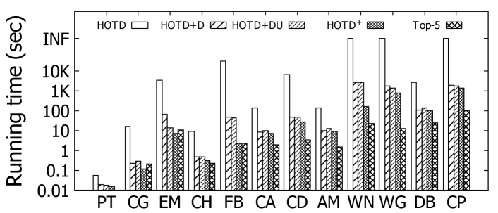
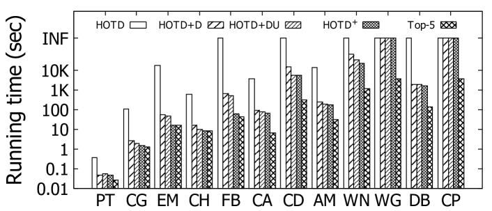
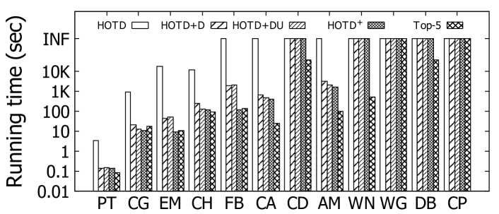
Exp-1: Efficiency of our proposed algorithms. In this experiment, we compare the running time of five algorithms on all datasets when $\tau$=2,3,4. The results are shown in Figure 6.

As $\tau$ increases, the running time of the algorithms increases as well. Regarding the algorithms, $\mathsf{HOTD}$ is slowest among the five algorithms. $\mathsf{HOTD}$+$\mathsf{D}$ is much faster than $\mathsf{HOTD}$ benefited from the delayed update strategy. Moreover, with utilizing the unchanged support detection strategy, $\mathsf{HOTD}$+$\mathsf{DU}$ is further faster than $\mathsf{HOTD}$+$\mathsf{D}$. Afterwards, $\mathsf{HOTD^{+}}$ is more efficient than $\mathsf{HOTD}$+$\mathsf{DU}$. This is because $\mathsf{HOTD^{+}}$ adopts all three optimization strategies to reduce the number of edges that need to update their higher-order support. Compared with $\mathsf{HOTD}$, $\mathsf{HOTD^{+}}$ achieves up to 4 orders of magnitude speedup. Besides, compared with $\mathsf{HOTD^{+}}$, $\mathsf{HOTTopR}$ is suitable to compute the top $r$ results as it avoids lots of unnecessary computation related to the non-top-$r$ results in $\mathsf{HOTD^{+}}$.

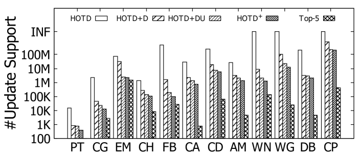
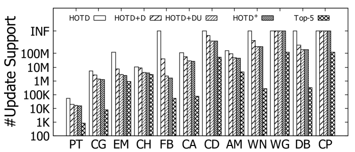
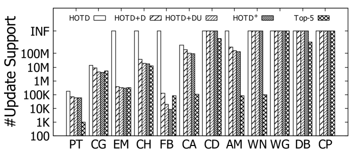
Exp-2: Number of higher-order support update. In this experiment, we report the number of higher-order support update of all algorithms during the decomposition when $\tau=2,3,4$. The results are shown in Figure 7.

As shown in Figure 7, on most datasets, the number of higher-order support updates of $\mathsf{HOTD}$ increase when $\tau$ increases from $2$ to $4$. This is because as the value of $\tau$ increases, the scope of edges that need update enlarges as well. However, the number of higher-order support update is significantly reduced by the optimization strategies. The results also explain the reasons causing different running times of the algorithms shown in Figure 6.

Table 2: Tightness of $\underline{\phi}_{\tau}(e,G)$

Dataset	$\tau$=2	$\tau$=3	$\tau$=4	Dataset	$\tau$=2	$\tau$=3	$\tau$=4
$\mathsf{PT}$	0.02	0.16	0.20	$\mathsf{CD}$	0.06	0.60	-
$\mathsf{CG}$	0.03	0.36	0.31	$\mathsf{AM}$	0.11	0.39	0.36
$\mathsf{EM}$	0.34	0.49	0.03	$\mathsf{WN}$	0.03	0.09	-
$\mathsf{CH}$	0.07	0.54	0.47	$\mathsf{WG}$	0.06	-	-
$\mathsf{FB}$	0.002	0.06	0.10	$\mathsf{DB}$	0.01	0.15	-
$\mathsf{CA}$	0.07	0.27	0.28	$\mathsf{CP}$	0.15	-	-

(a) $\mathsf{Random}$ $\mathsf{graphs}$ ($\tau$=2)

(b) $\mathsf{Random}$ $\mathsf{graphs}$ ($\tau$=3)

(c) $\mathsf{Random}$ $\mathsf{graphs}$ ($\tau$=4)

Figure 8: Scalability on synthetic random graphs

(a) $\mathsf{Power}$-$\mathsf{law}$ $\mathsf{graphs}$ ($\tau$=2)

(b) $\mathsf{Power}$-$\mathsf{law}$ $\mathsf{graphs}$ ($\tau$=3)

(c) $\mathsf{Power}$-$\mathsf{law}$ $\mathsf{graphs}$ ($\tau$=4)

Figure 9: Scalability on synthetic power-law graphs

Exp-3: Tightness of $\underline{\phi}_{\tau}(e,G)$. In this experiment, we evaluate the tightness of the lower bound $\underline{\phi}_{\tau}(e,G)$ in $\mathsf{HOTD^{+}}$. We use the widely adopted approximation error (AE) to measure the tightness Golub and Loan (1996). The approximation error for $\underline{\phi}_{\tau}(e,G)$ is defined as follows:

$$AE(\underline{\phi}_{\tau}(e,G))=\frac{\sum_{i=1}^{m}{\frac{|\phi_{\tau}(e_{i},G)-\underline{\phi}_{\tau}(e_{i},G)|}{\phi(e_{i},G)}}}{m};$$ (1)

As shown in Table 2, for $\underline{\phi}_{\tau}(e,G)$, when $\tau=2$, on most datasets, the approximation error is even less than 0.1, like $\mathsf{PT}$, $\mathsf{CG}$, $\mathsf{FB}$, $\dots$. When $\tau=3$, although its performance is not as good as that of $\tau=2$, the approximation error is still small on most datasets. This is because the $3$-hop neighborhood information is much more complex than the $2$-hop neighborhood information. When $\tau=4$, it shows a trend similar to that of $\tau=3$. Therefore, $\underline{\phi}_{\tau}(e,G)$ is effective regarding $\phi_{\tau}(e,G)$.

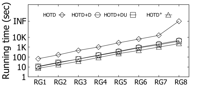
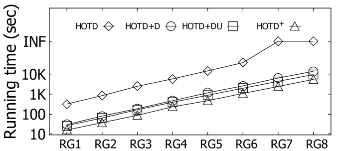
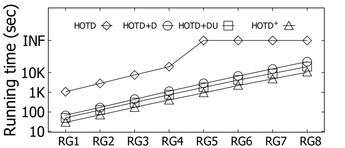
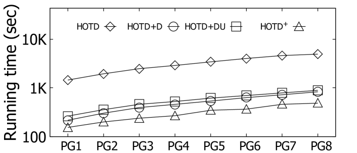
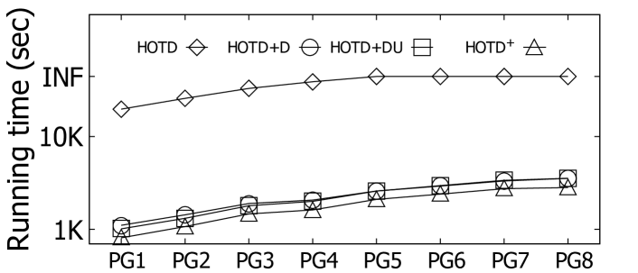
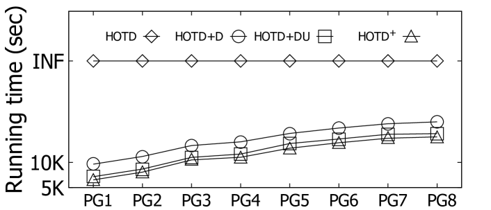
Exp-4: Scalability. Finally, we evaluate the scalability of the proposed algorithms on two kinds of synthetic datasets (random graph and power-law graph). For the random graph, we generates 8 graphs varying the number of vertices from $2^{17}$ to $2^{24}$ using the method in Holtgrewe et al. (2010); Meyerhenke et al. (2017). For the power-law graph, we generates 8 graphs varying the number of vertices from $3M$ to $10M$ using the method in Lancichinetti et al. (2008) (average degree with 10, other parameters with default setting). Figure 8 and Figure 9 show the running time of algorithms on random synthetic graphs and power-law synthetic graphs, respectively.

Figure 8 and Figure 9 show that as the graph size increases, the running time of all algorithms increases as well. This is because as the size of graphs increases, more edges have to be processed during the decomposition. Besides, for $\tau=2,3,4$, benefited from the proposed optimization strategies, $\mathsf{HOTD^{+}}$ is the most efficient one among the four algorithms and shows good scalability compared with other three algorithms.

(a) $\mathsf{Highschool}$

(b) $\mathsf{Political}$ $\mathsf{Books}$

Figure 10: Compare ($k$,$\tau$)-truss with ($k$,$h$)-core, hop=2

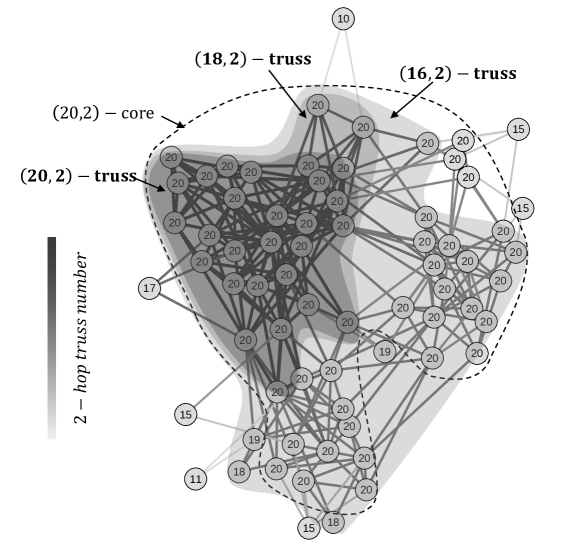
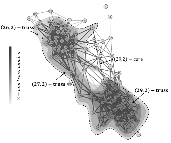
Exp-5: Case study. In this experiment, we compare ($k$,$\tau$)-truss with ($k$,$h$)-core which is the existing most similar cohesive subgraph model with our model. Figure 10 shows the differences between them on two real-world graphs $\mathsf{Highschool}$ and $\mathsf{Polotical}$ $\mathsf{Books}$ from KONECT. $\mathsf{Highschool}$ is a network contains friendships between boys in a small highschool. $\mathsf{Polotical}$ $\mathsf{Books}$ is a network of books, edges between books represent frequent co-purchasing of books by the same buyers. As shown at Figure 10(a), for ($k$,$h$)-core, most vertices are covered by (20,2)-core, it is hard to further distinguish more cohesive structure from it. For our model, (20,2)-core is further decomposed into more fine-grained hierarchy structure, like (16,2)-truss, (18,2)-truss and (20,2)-truss. Obviously, (20,2)-truss is the most cohesive subgraph through graph visualization. Figure 10(b) shows the similar phenomenon on $\mathsf{Polotical}$ $\mathsf{Books}$ dataset. It’s because a ($k$+1,$\tau$)-truss is a ($k$,$h$)-core but not vice versa, $\tau$=$h$. Therefore, our model can further search “core” of a ($k$,$h$)-core benefited from the more rigorous requirement for cohesiveness. In a result, our ($k$,$\tau$)-truss has higher ability to reveal fine-grained structure information.

8 Related Work

Truss decomposition. In the literature, plenty of research efforts have been devoted to the cohesive subgraph models for graph structure analysisLuce (1950a); Seidman (1983); Bonchi et al. (2019); Cohen (2008); Abello et al. (2002); Pei et al. (2005); Wang et al. (2010); Zhou et al. (2012); Wen et al. (2019). Among these cohesive subgraph models, the $k$-truss model has received considerable attention. $k$-truss model is first introduced in Cohen (2008). In Cohen (2008), an in-memory algorithm to detect the $k$-truss for a given $k$ with time complexity $O(\sum_{v\in V(G)}d^{2}_{1}(v,G))$ is proposed. Shao et al. (2014) studies the problem of detecting the $k$-truss for a given $k$ in distribute environments. By using the triangle counting techniques proposed in Latapy (2008), Wang and Cheng (2012) proposes an truss decomposition algorithm with time complexity $O(m^{\frac{3}{2}})$. Wang and Cheng (2012) also investigates the external-memory algorithms to conduct the truss decomposition. Zhang and Yu (2019) proposes an efficient algorithm to maintain the truss decomposition results in evolving graphs. Huang et al. (2016) investigates the truss decomposition problem in probabilistic graphs. Compared with our $(k,\tau)$-truss model, all these models only consider the direct neighbors of an edge and the higher-order neighborhood information is missed.

Distance-generalized cohesive subgraph models. Clique Luce (1950a), $k$-core Seidman (1983); Bonchi et al. (2019) and $k$-truss Cohen (2008) are three most fundamental cohesive subgraph models. For clique model, Luce (1950b); Moradi and Balasundaram (2018) propose two distance-generalized clique models, named $h$-club and $h$-clique. An $h$-club is a maximal subgraph $C$, s.t., the length of the shortest path between any two vertices of $C$ is not greater than $h$. The only difference between $h$-club and $h$-clique is that the shcortest path is within an $h$-club while it is not strictly necessary for $h$-clique. For $k$-core model, Batagelj and Zaveršnik (2011) proposes ($k$,$h$)-core model which requires each vertex in it has more than $k$ neighbors within $h$-hop neighborhood. Bonchi et al. (2019) proposes the ($k$,$h$)-core decomposition algorithm with better performance compared with Batagelj and Zaveršnik (2011). However, as shown at the experiments part (Exp-5), our model can search ”core” of ($k$,$h$)-core with higher ability to reveal fine-grained structure information. Besides, there is no distance-generalized model based on $k$-truss before our model.

9 Conclusion

As a representative cohesive subgraph model, $k$-truss model has received considerable attention. However, the traditional $k$-truss model ignores the higher-order neighborhood information of an edge, which limits its ability to reveal fine-grained structure information of the graph. Motivated by this, in this paper, we propose the $(k,\tau)$-truss model and study the higher-order truss decomposition problem. We first propose a bottom-up decomposition paradigm for this problem. Based on the paradigm, we further explore three optimization strategies, namely delayed update strategy, early pruning strategy, and unchanged support detection strategy, to improve the decomposition performance. Moreover, we also devise an efficient algorithm to compute the top $r$ ($k$,$\tau$)-trusses, which is useful in practical applications. Our experimental results on real datasets and synthetic datasets show the efficiency, effectiveness and scalability of the proposed algorithms.

References

- Abello et al. [2002] James Abello, Mauricio GC Resende, and Sandra Sudarsky. Massive quasi-clique detection. In LATIN 2002: Theoretical Informatics, pages 598–612. 2002.
- Abu-El-Haija et al. [2019] Sami Abu-El-Haija, Bryan Perozzi, Amol Kapoor, Nazanin Alipourfard, Kristina Lerman, Hrayr Harutyunyan, Greg Ver Steeg, and Aram Galstyan. Mixhop: Higher-order graph convolutional architectures via sparsified neighborhood mixing. In Proceedings of ICML, pages 21–29, 2019.
- Akbas and Zhao [2017] Esra Akbas and Peixiang Zhao. Truss-based community search: a truss-equivalence based indexing approach. Proceedings of VLDB Endow., 10(11):1298–1309, 2017.
- Andrade et al. [2006] Roberto F. S. Andrade, José G. V. Miranda, and Thierry Petit Lobão. Neighborhood properties of complex networks. Phys. Rev. E, 73:046101, Apr 2006.
- Andrade et al. [2008] Roberto FS Andrade, José GV Miranda, Suani TR Pinho, and Thierry Petit Lobao. Characterization of complex networks by higher order neighborhood properties. The European Physical Journal B, 61(2):247–256, 2008.
- Batagelj and Zaveršnik [2011] V. Batagelj and M Zaveršnik. Fast algorithms for determining (generalized) core groups in social networks. Adv Data Anal Classif, 5:129–145, 2011.
- Bonchi et al. [2019] Francesco Bonchi, Arijit Khan, and Lorenzo Severini. Distance-generalized core decomposition. In Proceedings of SIGMOD, pages 1006–1023, 2019.
- Chang and Qin [2018] Lijun Chang and Lu Qin. Cohesive Subgraph Computation over Large Sparse Graphs Algorithms, Data Structures, and Programming Techniques. Springer, 2018.
- Chang et al. [2013] Lijun Chang, Jeffrey Xu Yu, Lu Qin, Xuemin Lin, Chengfei Liu, and Weifa Liang. Efficiently computing k-edge connected components via graph decomposition. In Proceedings of the SIGMOD, pages 205–216, 2013.
- Chen et al. [2020] Zi Chen, Long Yuan, Xuemin Lin, Lu Qin, and Jianye Yang. Efficient maximal balanced clique enumeration in signed networks. In WWW, pages 339–349. ACM / IW3C2, 2020.
- Cohen [2008] J. Cohen. Trusses: Cohesive subgraphs for social network analysis. In Technical report, National Security Agency, 2008.
- Colomer-de Simón et al. [2013] Pol Colomer-de Simón, M Angeles Serrano, Mariano G Beiró, J Ignacio Alvarez-Hamelin, and Marián Boguná. Deciphering the global organization of clustering in real complex networks. Scientific reports, 3:2517, 2013.
- Eades et al. [2017] Peter Eades, Seok-Hee Hong, An Nguyen, and Karsten Klein. Shape-based quality metrics for large graph visualization. Journal of Graph Algorithms and Applications, 21(1):29–53, 2017.
- Ellson et al. [2002] John Ellson, Emden Gansner, Lefteris Koutsofios, Stephen C. North, and Gordon Woodhull. Graphviz— open source graph drawing tools. In Petra Mutzel, Michael Jünger, and Sebastian Leipert, editors, Graph Drawing, pages 483–484, Berlin, Heidelberg, 2002. Springer Berlin Heidelberg.
- Golub and Loan [1996] Gene H. Golub and Charles F. Van Loan. Matrix Computations. The Johns Hopkins University Press, 1996.
- Holtgrewe et al. [2010] Manuel Holtgrewe, Peter Sanders, and Christian Schulz. Engineering a scalable high quality graph partitioner. In 24th IEEE International Symposium on Parallel and Distributed Processing, IPDPS 2010, Atlanta, Georgia, USA, 19-23 April 2010 - Conference Proceedings, pages 1–12. IEEE, 2010.
- Huang et al. [2014] Xin Huang, Hong Cheng, Lu Qin, Wentao Tian, and Jeffrey Xu Yu. Querying k-truss community in large and dynamic graphs. In Proceedings of SIGMOD, pages 1311–1322, 2014.
- Huang et al. [2016] Xin Huang, Wei Lu, and Laks V. S. Lakshmanan. Truss decomposition of probabilistic graphs: Semantics and algorithms. In Proceedings of SIGMOD, pages 77–90, 2016.
- Lancichinetti et al. [2008] Andrea Lancichinetti, Santo Fortunato, and Filippo Radicchi. Benchmark graphs for testing community detection algorithms. In Phys. Rev. E 78, 2008.
- Latapy [2008] Matthieu Latapy. Main-memory triangle computations for very large (sparse (power-law)) graphs. Theory Computer Science, 407(1-3):458–473, 2008.
- Lee et al. [2010] Victor E. Lee, Ning Ruan, Ruoming Jin, and Charu C. Aggarwal. A survey of algorithms for dense subgraph discovery. In Managing and Mining Graph Data, pages 303–336. 2010.
- Liu et al. [2019a] Boge Liu, Long Yuan, Xuemin Lin, Lu Qin, Wenjie Zhang, and Jingren Zhou. Efficient (, )-core computation: an index-based approach. In WWW, pages 1130–1141. ACM, 2019.
- Liu et al. [2019b] Songtao Liu, Lingwei Chen, Hanze Dong, Zihao Wang, Dinghao Wu, and Zengfeng Huang. Higher-order weighted graph convolutional networks. CoRR, abs/1911.04129, 2019.
- Liu et al. [2020a] Boge Liu, Long Yuan, Xuemin Lin, Lu Qin, Wenjie Zhang, and Jingren Zhou. Efficient (, )-core computation in bipartite graphs. VLDB J., 29(5):1075–1099, 2020.
- Liu et al. [2020b] Qing Liu, Minjun Zhao, Xin Huang, Jianliang Xu, and Yunjun Gao. Truss-based community search over large directed graphs. In Proceedings of SIGMOD, pages 2183–2197, 2020.
- Luce and Perry [1949] R Duncan Luce and Albert D Perry. A method of matrix analysis of group structure. Psychometrika, 14(2):95–116, 1949.
- Luce [1950a] R Duncan Luce. Connectivity and generalized cliques in sociometric group structure. Psychometrika, 15(2):169–190, 1950.
- Luce [1950b] R.D Luce. Connectivity and generalized cliques in sociometric group structure. Psychometrika, 15:169–190, 1950.
- Meyerhenke et al. [2017] Henning Meyerhenke, Peter Sanders, and Christian Schulz. Parallel graph partitioning for complex networks. IEEE Trans. Parallel Distributed Syst., 28(9):2625–2638, 2017.
- Mones et al. [2012] Enys Mones, Lilla Vicsek, and Tamás Vicsek. Hierarchy measure for complex networks. PLOS ONE, 7, 03 2012.
- Moradi and Balasundaram [2018] Esmaeel Moradi and Balabhaskar Balasundaram. Finding a maximum k-club using the k-clique formulation and canonical hypercube cuts. Optim. Lett., 12(8):1947–1957, 2018.
- Orsini et al. [2013] Chiara Orsini, Enrico Gregori, Luciano Lenzini, and Dmitri Krioukov. Evolution of the internet -dense structure. IEEE/ACM Transactions on Networking, 22(6):1769–1780, 2013.
- Ouyang et al. [2020] Dian Ouyang, Long Yuan, Lu Qin, Lijun Chang, Ying Zhang, and Xuemin Lin. Efficient shortest path index maintenance on dynamic road networks with theoretical guarantees. Proc. VLDB Endow., 13(5):602–615, 2020.
- Pei et al. [2005] Jian Pei, Daxin Jiang, and Aidong Zhang. On mining cross-graph quasi-cliques. In Proceedings of SIGKDD, pages 228–238, 2005.
- Sahu et al. [2017] Siddhartha Sahu, Amine Mhedhbi, Semih Salihoglu, Jimmy Lin, and M. Tamer Özsu. The ubiquity of large graphs and surprising challenges of graph processing. Proc. VLDB Endow., 11(4):420–431, 2017.
- Seidman [1983] Stephen B Seidman. Network structure and minimum degree. Social Networks, 5(3):269–287, 1983.
- Shao et al. [2014] Yingxia Shao, Lei Chen, and Bin Cui. Efficient cohesive subgraphs detection in parallel. In Proceedings of SIGMOD, pages 613–624, 2014.
- Sun et al. [2020] Zequn Sun, Chengming Wang, Wei Hu, Muhao Chen, Jian Dai, Wei Zhang, and Yuzhong Qu. Knowledge graph alignment network with gated multi-hop neighborhood aggregation. In Proceedings of AAAI, pages 222–229, 2020.
- Wang and Cheng [2012] Jia Wang and James Cheng. Truss decomposition in massive networks. Proceedings of VLDB Endow., 5(9):812–823, 2012.
- Wang et al. [2010] Nan Wang, Jingbo Zhang, Kian-Lee Tan, and Anthony K. H. Tung. On triangulation-based dense neighborhood graphs discovery. Proceedings of VLDB Endow., 4(2):58–68, 2010.
- Wen et al. [2019] Dong Wen, Lu Qin, Ying Zhang, Lijun Chang, and Ling Chen. Enumerating k-vertex connected components in large graphs. In Proceedings of ICDE, pages 52–63, 2019.
- [42] Xudong Wu, Long Yuan, Xuemin Lin, Shiyu Yang, and Wenjie Zhang. Towards efficient k-tripeak decomposition on large graphs. In DASFAA.
- Xue et al. [2020] Hui Xue, Xin-Kai Sun, and Wei-Xiang Sun. Multi-hop hierarchical graph neural networks. In Proceedings of BigComp, pages 82–89, 2020.
- Yuan et al. [2016a] Long Yuan, Lu Qin, Xuemin Lin, Lijun Chang, and Wenjie Zhang. Diversified top-k clique search. VLDB J., 25(2):171–196, 2016.
- Yuan et al. [2016b] Long Yuan, Lu Qin, Xuemin Lin, Lijun Chang, and Wenjie Zhang. I/O efficient ECC graph decomposition via graph reduction. Proc. VLDB Endow., 9(7):516–527, 2016.
- Yuan et al. [2017] Long Yuan, Lu Qin, Xuemin Lin, Lijun Chang, and Wenjie Zhang. Effective and efficient dynamic graph coloring. Proc. VLDB Endow., 11(3):338–351, 2017.
- Yuan et al. [2018] Long Yuan, Lu Qin, Wenjie Zhang, Lijun Chang, and Jianye Yang. Index-based densest clique percolation community search in networks. IEEE Trans. Knowl. Data Eng., 30(5):922–935, 2018.
- Zhang and Yu [2019] Yikai Zhang and Jeffrey Xu Yu. Unboundedness and efficiency of truss maintenance in evolving graphs. In Proceedings of SIGMOD, pages 1024–1041, 2019.
- Zhou et al. [2012] Rui Zhou, Chengfei Liu, Jeffrey Xu Yu, Weifa Liang, Baichen Chen, and Jianxin Li. Finding maximal k-edge-connected subgraphs from a large graph. In Proceedings of EDBT, pages 480–491, 2012.