Does it work outside this benchmark? Introducing the Rigid Depth Constructor tool, depth validation dataset construction in rigid scenes for the masses

Abstract

We present a protocol to construct your own depth validation dataset for navigation. This protocol, called RDC for Rigid Depth Constructor, aims at being more accessible and cheaper than already existing techniques, requiring only a camera and a Lidar sensor to get started. We also develop a test suite to get insightful information from the evaluated algorithm. Finally, we take the example of UAV videos, on which we test two depth algorithms that were initially tested on KITTI [34] and show that the drone context is dramatically different from in-car videos. This shows that a single context benchmark should not be considered reliable, and when developing a depth estimation algorithm, one should benchmark it on a dataset that best fits one’s particular needs, which often means creating a brand new one. Along with this paper we provide the tool with an open source implementation and plan to make it as user-friendly as possible, to make depth dataset creation possible even for small teams. Our key contributions are the following: We propose a complete, open-source and almost fully automatic software application for creating validation datasets with densely annotated depth, adaptable to a wide variety of image, video and range data. It includes selection tools to adapt the dataset to specific validation needs, and conversion tools to other dataset formats. Using this application, we propose two new real datasets, outdoor and indoor, readily usable in UAV navigation context. Finally as examples, we show an evaluation of two depth prediction algorithms, using a collection of comprehensive (e.g. distribution based) metrics.

1 Introduction

Using computer vision for navigation has long been well established, as a camera sensor is very easy to set up, cheap and power efficient. The main uses are for odometry and 3D maps which are then used to control the navigation, especially find a path and avoid obstacles.

Estimating depth from a camera is not an easy task, and validation data is very hard to obtain. Indeed, knowing depth requires to know the 3-dimensional environment the camera is facing with respect to its position. This requires to explicitly measure depth with range sensors like Lidar or ToF cameras.

A major example of depth validation dataset is KITTI [8], where a set of cameras and a Lidar are mounted on a car. Following the acquisition, the Lidar and video signals are calibrated and synchronized in order to construct sparse depth maps for every camera at every moment. The main problem with this method is that you need to construct a rigid rig between a Lidar and a camera, which, in addition to being very costly can become very heavy, and is not suitable to recreate the natural movement of a handheld camera or a consumer UAV camera.

To address this problem, we propose a way to construct a depth dataset with a two-step method that first uses a Lidar to scan an environment and then localizes images from a video camera with respect to the Lidar point cloud. Our method aims at being the most user friendly possible, and with maximal flexibility, both on the methods to construct the point cloud, and on the type of camera used for acquisition.

Along with this paper, we provide the tool as an open source package thoroughly tested with an industrial research team to ensure its usability. We will present the general method that is widely inspired from ETH3D [31], and present three use cases that we were able to construct. Finally, we will use these datasets to show with a benchmark on monocular depth estimation algorithms that results can vary greatly depending on the context and that the in-car environment, well referenced through the KITTI benchmarks, is far from being representative of all navigation use cases. This means that for each new navigation scenario, a new dataset should be constructed, at least for validation, which is exactly what our tool aims at making easier and cheaper.

2 Related works

2.1 Depth estimation for navigation

Depth estimation, and more generally 3D perception is a core task for autonomous navigation. In the context of very light vehicles such as UAV, that can’t carry heavy hardware, depth is often deduced from one or multiple cameras. The stereo camera is often used to compute depth from disparity [20], that can also be estimated with a single camera, which has the advantage of being much cheaper to integrate. Depth can then be deduced from motion, by using methods based on epipolar geometry [11]. Structure from motion and SLAM techniques can then be used to deduce both depth and camera movement using only optical flow and geometric equations. It must be noted that all structure from motion algorithms require rigid scenes, i.e. without moving objects.

More recently, depth inference networks have been shown to be able to estimate depth from a single image solely from perspective and context. Indeed, with only one image, they were able to get reasonable scale invariant (i.e. relative depth maps) quality measures [6, 17, 26, 5, 36]. However, in a navigation context, the scale invariant quality is not really interesting without a way to link the estimation to the real world. Instead of relative or normalized values, absolute depths are needed for a navigation algorithm such as Model Predictive Control [18] to be used. To this end, depth algorithms need to estimate both depth and movement in order to work for navigation. Among the examples mentioned above, Zhou et al. [36] is the only one we can work with. It is important to note that depth from a single image does not use pixel displacements. It is deemed a more bio-inspired method which makes use of end-to-end training of convolutional neural networks and their capacity of generalizing implicit pixel structure, but it does not rely on elaborate geometric constraints. As such, it is expected to be less robust for unusual scene, especially with a confusing perspective.

2.2 Validation sets and benchmarks: the specific case of consumer UAV cameras, or why we need a new dataset

This project was mostly motivated by the specific use case of depth estimation from UAV consumer drone, which lacks a proper validation dataset. Indeed, most depth algorithms are currently tested either for autonomous driving environments such as KITTI [34], or indoor environment such as NYUv2 [21]. In these evaluation frameworks, single image depth prediction algorithms heavily prevail within the leaderboard, which makes these techniques de facto state of the art.

As shown in [24], the context of UAV navigation is much more heterogeneous than these environments, both in terms of camera pose and surrounding environment. However, contrary to KITTI, the problem of moving objects is deemed (at least for now) a secondary problem when flying high above the ground. It is thus not certain that algorithms performing well on KITTI or NYUv2 will not perform poorly in this context. This is especially true when considering that moving objects in KITTI make depth from motion much harder, while depth from context is not robust enough to the viewpoint variability. As such, these datasets address issues for particular use cases with their own difficulties that are not reflected in the UAV use case and vice-versa. This idea is corroborated by the fact that the Sintel depth dataset [2] remains largely unsolved for the moment because in addition to moving objects, scene heterogeneity is much more prevalent.

Inspired by the Flying Chairs synthetic dataset for optical flow[4], which is founded on a surrealistic abstraction of the difficulties of optical flow, Still Box [23] has been proposed. It is a synthetic dataset trying to recreate the difficulties of a UAV flight, focusing on heterogeneity of appearance, using random shapes and textures. As such, it is a good training dataset, the same way Flying chairs is a good training dataset for optical flow, but obviously, it is not suited for evaluation. Table 1, which compares the difficulties of the datasets currently used as benchmarks for depth quality, shows that none of them is relevant for the UAV camera use case.

	KITTI[34]	NYUv2[21]	Sintel Depth[2]	Still Box [23]	a good UAV dataset
Moving objects	✓	✗	✓	✗	✗
Outdoor	✓	✗	✓	N/A	✓
Camera orientation variation	✗	✓	✓	✓	✓
Camera position variation	✗	✗	✓	✓	✓
Real videos	✓	✓	✗	✗	✓

Table 1: Difficulties featured in existing datasets. Being non photo-realistic, the distinction between Indoor and Outdoor is irrelevant for Still Box.

2.3 Constructing a depth enabled dataset

The basic principle of depth enabled dataset construction is to use a device with reliable depth estimation capability, that won’t be available during evaluation. Typically, we can use a rig with a RGB camera and a depth sensor like structured light [21], Time of Flight, embedded Lidar [34, 35], or light-field camera grids [27]. For evaluation, only the camera will be available, and the evaluation step will then measure the agreement between ”reliable depth” measured by the dedicated sensor and estimated depth. It is important to note that an evaluation is only informative up to a certain point, where the quality of both methods are comparable. For dedicated depth sensors, we usually rely on the vendor’s datasheet. However, this solution requires that we can emulate the camera movement of the use case we are trying to cover, i.e. without potentially heavy depth sensors. This is problematic for consumer UAV, because the typical movement of its camera is difficult to mimic. Not only the camera is well stabilized, with a very smooth trajectory, that is not reproducible by hand, but the size of these cameras make it easy to fly very close to obstacles, which is not reproducible by a heavier UAV that could carry an additional depth sensor. These kinds of UAVs are usually very dangerous and need to be operated far from obstacles.

An interesting method for rigid scenes has been presented with ETH3D [31] and Tanks and Temples [13] that usually serve to evaluate photogrammetry. Instead of having a depth sensor and a camera attached to the same rig, the data acquisition is done in two steps. They first get a point cloud measure from fixed laser scanners such as the FARO Focus, and then take images from cameras in the same scene after removing the laser scanner. This implies that no object is moving in the scene, but allows for any camera to be used. In the particular case of ETH3D, they added a photogrammetry step, using the taken pictures and some RGBD rendering of the Lidar scanner with the COLMAP software [28]. This allowed them to get frame localization with respect to each other, but also with respect to the Lidar scanner position. With this technique, they were able to get depth map indirectly from the Lidar point cloud. They then used the generated depth map and camera position to get a stereo validation, with rectified frames. The ETH3D dataset construction method has been used as a foundation of our framework. Our goal is to generalize their method not only for photogrammetry oriented footage, but for all kinds of videos, using anything available to acquire a 3D point cloud of a scene.

3 Dataset creation method

3.1 The foundations: COLMAP and ETH3D

ETH3D already offers to compute depth maps from a Lidar point cloud and a separate camera, but it has been used in a very particular context and some of its methods are not suited for a more general one. Because this article aims at using the same tools as ETH3D, we analyze them and indicate what aspects need to be changed in order to increase flexibility.

3.1.1 Photogrammetry with COLMAP

COLMAP [30, 28] is a photogrammetry tool designed to be very robust, in order to reconstruct a 3D model from crowdsourced images taken from the internet. To go from a set of images to a 3D model with images localization, the steps applied are presented in Fig. 1. The main problem of COLMAP is that even if the matching process can be dramatically accelerated with vocabulary tree matching [29], it is still in $\mathcal{O}(n^{3})$ where $n$ is the number of images. As such, the reconstruction process can be very long for videos.

Figure 1: Photogrammetry workflow used in COLMAP. Note that the mapping process can stop at ”Image registration” and the Delaunay mesher accepts any point cloud as long as the visibility index is correct.

3.1.2 Depth generation with ETH3D

ETH3D [31] uses COLMAP to localize calibrated images with respect to a Lidar point cloud taken with a FARO Focus. The FARO Focus is a fixed point Lidar that renders colored 3D points. Since it is fixed, every 3D point is measured from the same origin. This device allows them to synthesize high quality depth-valued images with known position of the scanner (i.e. the cloud origin) that can be integrated in the COLMAP reconstruction process. The position of each image is thus known with respect to the point cloud. Each image then gets its position refined by matching feature points between real images and rendered images from the colored point cloud of an equivalent camera at the estimated position. However, the localisation part is not usable for our use case, because we want to be able to use any point cloud, i.e. without colors. We can note that, as it is stated by their paper, the localization step can be done when simply constructing a 3D model with COLMAP and then register it with respect to the Lidar point cloud, with e.g. ICP [1].

Once the Images are localized with respect to Lidar, the depth rendering part is detailed in Figure 2. Mainly, in addition to image calibration and localization, an occlusion mesh needs to be computed from the point cloud, which is then used to construct an occlusion depth. This depth map is significantly worse than the one from the point cloud, but it is only used to determine occlusion (and thus point visibility) and then avoid the ghosting effect of seeing through a 3D object due to the sparsity of the point cloud. To this occlusion mesh we can add the ”splats”, which are created from isolated points: assuming such points are representative of thin objects (such as the leg of a chair), they may not be represented by the occlusion mesh but still count as occluding point, the splat creator is used to construct oriented squares at the point position, in order to avoid the risk of rendering depth values of a background object for the rest of the thin object.

In ETH3D[31], the occlusion mesh is constructed with Poisson algorithm [12]. This supposes that point normals can be computed and oriented. Again, this is possible with point clouds coming from a fixed laser scanner where normals are always oriented toward the origin, but it is not always the case for unstructured point clouds. We will then have to find an alternative solution.

Figure 2: Photogrammetry workflow used with ETH3D. Note that this workflow does not include localization, which is much more complicated but is not available to us, since we assume that we don’t necessarily have a colored point cloud.

3.2 Changing the ETH3D workflow

The constraints from the ETH3D use case context can be summarized this way:

• The number of images is very small. However if we want to use videos, we might have thousands of frames to localize.

• The Lidar is a very high quality color-enabled fixed scanner. However we want to be able to use any collection of unordered point clouds, for which the computation of the mesh is much harder.

In short, we need to find a way to localize images with COLMAP in linear time while keeping a good 3D reconstruction, and we need a way to construct a good mesh from unordered point clouds.

3.2.1 Extending COLMAP reconstruction

The issue regarding the number of images can be solved by simply using a subset of images for reconstruction. The reconstruction needs to be good enough to be precisely registered with respect to the Lidar point cloud. For a small subset of frames, the full structure from motion mapping process can be applied even if it is very expensive. However, for remaining frames, the 3D point cloud will only be marginally better since their views are supposedly already covered by nearby frames. We can then afford to only register with respect to the already existing reconstruction. This process is much less expensive, as it does not need to perform a global bundle adjustment at each frame.

The issue is now to choose a good subset of frames. This can be solved during the data acquisition step. Indeed, we can take a set of pictures dedicated to photogrammetry following guidelines in [14]. The goal is, for a fixed number of pictures to be used in the mapping process, to have pictures with the most uniformly distributed position and orientation view points. This can be done for example with a UAV orbiting around a particular object or flying along a grid above the scene: pictures are sampled at a regular pace to ensure a good parallax between images.

3.2.2 Constructing the Occlusion mesh

In the hypothesis we were successful in localizing every image with respect to the Lidar point cloud, we can use a specific tool to construct a mesh. After point cloud densification with multi view synthesis and depth maps fusion, COLMAP outputs a point cloud with normals and a visibility index indicating from which frame each 3D point is visible. These two features are used for mesh reconstruction. Indeed, as discussed earlier, Poisson reconstruction [12] can be used thanks to normals, and Delaunay meshing [16] can be used with visibility index. If we make the unrealistic assumption that both dense reconstruction from COLMAP and Lidar point cloud are perfect, we can easily transfer these features from one cloud to another. Although COLMAP is known to have a low recall, by discarding many points in textureless areas, in our experiments, we found that transferring feature from the nearest neighbor of each Lidar point was sufficient.

3.3 Our final workflow

The final version of our workflow can be found in Figure 3, that represents the complete algorithm needed for ground truth creation from ETH3D. We now present it in details.

Figure 3: Simplified representation of our workflow before using ETH3D tools. Video frames get registered with respect to the reconstruction point cloud, along with the Lidar point cloud. As such, we can use ETH3D with the COLMAP model, the Occlusion mesh and the registered Lidar point cloud.

3.3.1 Data acquisition and ground truth point cloud creation

In order for our protocol to be easy to follow, this part is very open and only asks for a point cloud of the scene, acquired by any mean, and not necessarily colored. The point cloud will be used as a perfect ground truth, which means that subsequently constructed depth maps can only be as precise as this point cloud. As suggested by [31], a tripod fixed Lidar scanner can be used in order to have the maximum precision and density (precision at the millimeter level). However, other Lidar sensors can be used, such as mobile Lidars attached to a UAV, or a human handle. Although they lack precision (which is now at the centimeter level), their ease of use can be leveraged to have a much more complete point cloud, especially in cluttered environments or unreachable places like a building’s roof. As a last resort, when no Lidar is available, even the result of a photogrammetry can be used, in order to compare a real-time depth algorithm to a thorough reconstruction algorithm that does not sacrifice quality for speed. Throughout this section, the point cloud that serves as a ground truth is referred to as Lidar point cloud, but everything applies the same for any other ground truth point cloud creation method.

3.3.2 First thorough photogrammetry

This first step uses COLMAP to construct a photogrammetry comprising a point cloud and the viewpoint position of every image that was successfully localized. The reconstructed point cloud will then be localized with respect to the ground truth point cloud. Note that this step is different from ETH3D since we don’t necessarily have a colored point cloud, and thus cannot synthesize images from Lidar data.

As said above, our goal is to make model reconstruction as efficient as possible. If we had to use all the video frames we want to localize, the reconstruction would be comprehensive, but also extremely long. Instead, in addition to the ”photogrammetry frames”, we only include a subset of each wanted video to the photogrammetry process, so that the reconstruction is not too long while including sufficient number of different view points. The sampling can be based on frame rate (e.g. only take one frame per second), but it is not ideal when the camera is not moving. In the case of frames with displacement metadata, we can sample a more efficient subset by using K-means [19] on a 6D point cloud composed of frames positions and orientation. Note that the importance of orientation in sampling can be parameterized by weighting the orientation coordinates in the 6D point cloud.

3.3.3 Registration of ground truth point cloud with respect to the output of photogrammetry

This step requires to find the optimal rigid transformation (rotation, translation and scale) between the reconstructed point cloud and the Lidar point cloud. Assuming COLMAP’s reconstruction is good enough, a simple ICP [1] or related algorithm like point-to-plane ICP [3] can be used to align the two point clouds. It is probably the most sensitive step of the process, and requires a human supervision.

Indeed, ICP is a somewhat unstable process that needs assessment and a good initialization. As such, a human needs to thoroughly check the point cloud alignment and manually estimate a first rough transformation, with e.g. point pair picking. This can be done by e.g. meshlab or Cloudcompare .

3.3.4 Video localization

This step only uses the image registration tool from COLMAP applied to the existing reconstruction. It does not contribute to the point cloud reconstruction, and only uses local bundle adjustment to localize the frame with its neighbors. As such, this operation is much faster than the whole reconstruction process, where point triangulation and global bundle adjustment was used.

3.3.5 Localization filtering

The main interest of COLMAP compared to other SLAM method is that everything is global. This way every frame is not only localized with respect to its neighbors, but also with respect to any other frame with which it shares a sufficient field of view. As such, if each video frame contains features matched in enough well globally localized photogrammetry frames, the localization does not drift with respect to the reconstruction. However, since odometry is not perfect either, we can end up with a noisy trajectory that would not be possible for a real camera with bounded acceleration. This is especially true for consumer UAVs which usually focus on video smoothness using a stabilized guimbal, for aesthetic purposes.

To reflect this observation, on each localized video, we apply a Savitzky-Golay filter [25] to both trajectory and orientation. This filter not only smoothes the movement, but also helps detecting outlier that were badly localized. This way, we can discard the frames for which the distance between estimated and filtered 6D positions is above a certain threshold, and interpolate their position from neighboring frames. These frames will not be used for depth evaluation, but can be used e.g. for depth algorithms that rely on odometry.

3.3.6 Depth and pose ground truth generation

Finally, we use the ground truth creator developed for ETH3D [31] to construct depth maps for all the video frames. We now have a ground truth for odometry and depth for each successfully localized frame.

3.3.7 Dataset conversion and evaluation subset creation

Now that we have images with odometry and depth, we can convert the dataset format in compliance with more popular datasets. For example, we can use the same format as KITTI odometry, in order to ease validation of depth algorithms on new datasets.

In addition, the same way Eigen[5] proposed an evaluation split for depth, we can set a list of frames that will be used for depth evaluation. Odometry can allow us to adapt our subset and its format to several evaluation scenarios:

• We can filter candidate frames according to the movement, e.g. only forward motion (like in the context of a car), or without rotation.

• For algorithms based on normalized (relative) depth with corresponding pose estimation with respect to previous frames (e.g. SFMLearner [36]), we can solve the scale factor with displacement magnitude, as suggested in [24].

• For algorithms that need odometry, such as multi view stereo, or algorithms that need frames with compensated rotation [24], it can be provided. This scenario is realistic for navigation context in the case of a UAV, where velocity and orientation need to be known primarily for a stable flight and a smooth video, and thus are available for these algorithms.

3.4 Automation

All the above processes have been included into a script that makes extensive use of COLMAP, ETH3D, PCL, and Parrot’s Anafi SDK. This script is intended to be as easy to use and as flexible as possible, in order to cover a wide range of use cases and budgets. It is open-sourced on Github with extensive usage documentation.

3.5 How good a ground truth can we hope to reach?

During the whole process, we have assumed that the 3D point cloud was perfect, or at least not improvable. We chose to trust precision ranges given by scanner vendors. For example for a fixed Lidar scanner such as the Faro Focus, the precision is below the centimeter, while for handheld Lidars such as Velodyne VLP16 used either with a UAV or handheld, the precision is below 5 centimeters. This means that depending on the device used for mapping, one needs to pay attention to the depth ranges seen during videos to be localized. This is particularly true for videos very close to obstacles, where the precision of depth maps measured by COLMAP’s patch match stereo step can be better than Lidar reference.

Using fixed or mobile scanners is then a trade-off between mobility, scan time, precision and completeness.

Regarding odometry, we consider the localization made by COLMAP to be perfect. It can be noted that this was not the case for ETH3D, where they applied a pose fine tuning for each frame. Unfortunately, their method is only available for colored point clouds, which is not the case for most mobile Lidars. This problem can be mitigated by two factors:

• The colorless scanners are also the less precise ones. As such, solving this problem might get negligible improvement since the point cloud quality will then become the limiting factor. Otherwise, we can simply apply ETH3D’s pose refinement technique.

• We tested COLMAP on EuroC dataset, and were surprised to see that odometry from the provided ground truth (measured with a Lidar scanner and an IMU) was not very good compared to odometry computed by COLMAP. This can be seen on Figure 4, where the triangulated 3d points are visibly much less noisy from COLMAP odometry than from ground truth. This is corroborated with the EuroC depth dataset proposed by [10], where synthesized depth maps from frame position and camera calibration were not exactly aligned with the camera, even in their illustrating figure (see Figure 5).

In sum, we have good, albeit subjective, reasons to think that the odometry from dedicated sensors is not necessarily needed compared to the one computed by COLMAP. We can only make a subjective manual assessment, but as mentioned in the first point, we believe that point cloud quality is often the limiting factor. However, we cannot ignore the fact that for some particular cases, such as a video that is isolated in a cluttered part of a scene and only connected to the rest of the photogrammetry by a few frames, the odometry can drift. This makes these localized frames misaligned with the Lidar point cloud, and thus with a poor ground truth depth, even if the Lidar point cloud registration step is optimal, because it’s only a rigid transformation. A solution to this problem could be to apply a non-rigid registration [33] of the COLMAP point cloud, deforming the cloud and then also the frame localization to fit the Lidar point cloud more precisely. This might be the occasion of a future work combining COLMAP’s bundle adjustment and cloud-to-cloud distance between COLMAP and Lidar point cloud. However, a more direct way of limiting this problem is to ensure during data acquisition that all video frames can be localized with a large number of photogrammetry oriented pictures, so that a ”loop closure” step is applied very often, with pictures designed to have a very precise localization with respect to the reconstruction cloud.

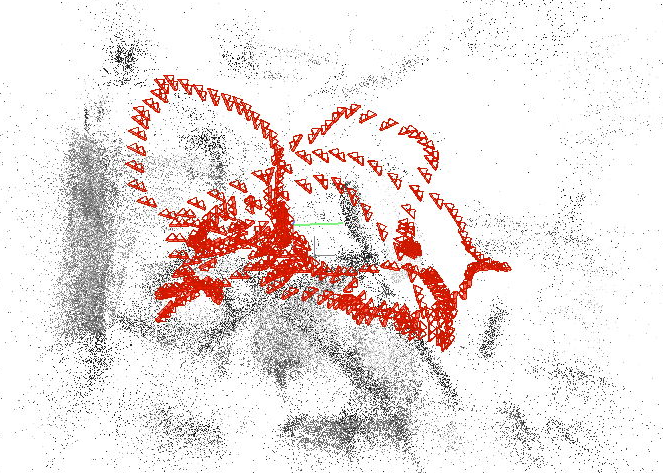
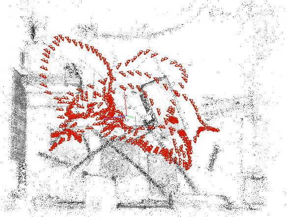
(a)	(b)

Figure 4: Visual qualitative assessment from COLMAP mapping process. (a) localization from available ground truth odometry, measured from Lidar and IMU. (b) localization deduced by COLMAP during the mapping process with SLAM. Visualization was done via COLMAP GUI.

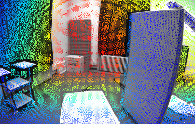
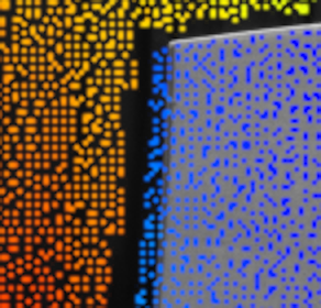
(a)	(b)

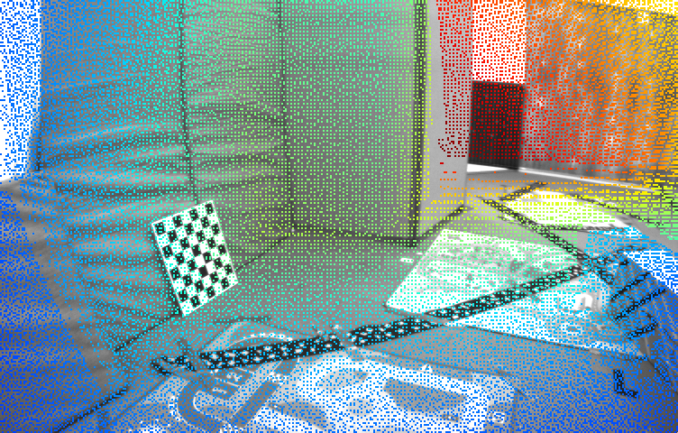
(c)

Figure 5: Depth map proposed by [10]. Image and colored depth maps are superposed to show the alignment problem, especially for foreground and background delimitation. (a) depth map shown in Figure SM2 of [10] (from their supplementary materials), with (b) zoom details. (c) depth map from another sequence, where alignment error is larger than 40 pixels.

4 Measuring depth quality for navigation purposes

Since we want to build an evaluation dataset, we are looking for the most informative metrics. As we are mostly interested in the context of navigation, we chose to follow the methodology proposed in [24]. Namely, contrary to the well used ”Eigen-split” [5], using metrics from Garg et al. [7], we want to apply a realistic navigation scenario, that requires the estimated depth to be absolute, and not up to a factor computed with the ratio of medians. This makes depth from single view algorithms unable to compete, unless there is a way to compute the scale factor by comparing odometry with actual displacement, which is much more realistic for any kind of autonomous vehicle. Single frames algorithms such as Deep Ordinal Regression Network (DORN) [6] or Big to Small (bts) [17] can thus not be used, but some other algorithms such as SFMLearner and its variants  [36, 9] are trained with a pose estimator and thus can be evaluated.

4.1 On the information a metric gives

Most of the time, for evaluation datasets, metrics are used for the only purpose of ranking different algorithms. This is useful for benchmarking and choosing an existing algorithm for one’s usage, but it raises some problems from the end user’s perspective:

• It does not reflect the context of the use case that might be different from the original validation set. For example, if someone wants to estimate depth from a single camera but only for close objects because the long range is already covered by another sensor, this user won’t be interested in long range depth estimation quality, and the metric used for benchmarking will have to reflect this.

• Some characteristics of an algorithm are inherently antagonistic, and thus a trade-off must be decided between them. The most usual example is accuracy vs speed. By ranking algorithms with only one metric, the dataset makes the trade-off decision in place of the end user and thus takes the risk of not being informative. For example, because speed is only given as declared from the authors, KITTI depth benchmark [34] completely disregards it. It would be interesting to have data presented into a 2D chart, the same way as VOT [15] so that the end user can eventually set his own speed/accuracy trade-off.

• A metric can give information about the distribution of expected values given a particular estimation. As such, as shown in  [22, p. 38] all metrics are not the same when it comes to trying to characterize possible real values of an estimation. The ideal solution would be to give for each estimated depth value the exact distribution of real depth. That would require an infinite set, but the validation set can give an approximation that gives more insight than just a single number.

To reflect those practices, we decide to have both a set of classic metrics and histograms to give as much information as possible for a given algorithm. Again, the code for metric measurement is open sourced on Github . It consists in getting all depth pixels and their estimation, within an unordered set $V$. Note that this evaluation set is not image-wise, all depth values are collected at first with corresponding metadata, and the metric computation is done at the end. This is useful for images with a very sparse depth, where no representative statistics can be computed.

4.2 Scalar metrics

A scalar metric is obtained by computing a depth errors for all points and then averaging them. As mentioned above, the mean is global over the validation set $V$:

$$\mathcal{E}_{f}=\frac{1}{|V|}\sum_{(\widetilde{\theta},\theta)\in V}f(\widetilde{\theta},\theta)=\mathbb{E}_{V}(f(\widetilde{\theta},\theta))$$

Where $\theta$ is the ground truth depth for a particular pixel, $\widetilde{\theta}$ its estimate, and $f$ the error function.

Table 2 shows provided error functions and corresponding names.

Error Name	Acronym	$\mathbb{E}(f(\widetilde{\theta},\theta))$
Mean Absolute Error	$MAE$	$\mathbb{E}|\widetilde{\theta}-\theta|$
Mean Relative Error	$MRE$	$\mathbb{E}\frac{|\widetilde{\theta}-\theta|}{\theta}$
Mean Log Error	$MLE$	$\mathbb{E}|\log(\widetilde{\theta})-\log(\theta)|$
Standard Absolute Error	$SAE$	$\sqrt{\mathbb{E}(\widetilde{\theta}-\theta)^{2}}$
Standard Log Error	$SLE$	$\sqrt{\mathbb{E}(\log(\widetilde{\theta})-\log(\theta))^{2}}$
Precisions $\delta$	$P_{\delta}$	$P\left(\left|\log\left(\frac{\widetilde{\theta}}{\theta}\right)\right|\leq\log(\delta)\right)$

Table 2: Considered Metrics Summary

4.3 Histogram metrics

Histogram metrics cannot be used for ranking algorithms but they give much more information. We propose two different histograms:

• Depth wise error: Given a scalar metric, we can compute the error for particular depth values.

  $$H_{D}(\theta_{0})=\mathbb{E}_{\{\theta=\theta_{0}\}}(f(\theta,\widetilde{\theta}))$$

• Difference distribution: This distribution is normally centered around $0$, and its standard deviation is the standard error mentioned on Table 2. Having the whole distribution is especially interesting for distribution that are not symmetrical. A safety interval can then be deduced from this histogram for each side of estimated depth. For this part, we follow the assumptions that the log of depth estimation is more likely to follow a symmetrical distribution than raw depth estimation. It is equivalent to get a distribution of the ratio between estimation and ground truth, usually centered around 1.

  $$H_{\Delta}(\delta)=P(\log(\widetilde{\theta})-\log(\theta)=\delta)=P\left(\frac{\widetilde{\theta}}{\theta}=10^{\delta}\right)$$

4.4 Displacement wise metrics

In addition to those metrics, we propose to have a displacement wise metric in the form of an histogram. Namely, if we know the displacement, we can deduce what point in the image the camera is moving toward to. This point, called the flight path vector (FPV) for aircraft, also corresponds to the epipole for multi-view geometry, and to the focus of expansion (FOE) for optical flow in the case of rotation-less movement. As a consequence, these points are deemed more important than the other ones.

$$\mathcal{E}_{FPV}(\alpha)=\mathbb{E}_{V(\alpha)}(f(\widetilde{\theta},\theta))$$

Where $V(\alpha)$ is the set of points at a distance $\alpha$ from the FPV of each image (be it in pixels, or in radians).

This particular distribution can help discard an algorithm that fails to estimate depth around those points while having good metrics otherwise. This is the case for optical flow based method for a stabilized camera without rotation: optical flow is too small around the FPV and thus disparity based depth estimation becomes too noisy. [22, p 32]

5 Applications

5.1 Preamble

In this section, we present two use cases we have covered using this tool. They both feature drone footage, and are used to test two algorithms: DepthNet [23] and SFMLearner [36]. They are not state of the art on popular benchmarks like KITTI[34], but they are relevant to demonstrate the interest of the proposed evaluation framework and data sets, for the following reasons:

• They are both compatible with our evaluation scenario focused on navigation, because we can scale their depth estimation only using odometry

• They are supposed to be real time, contrary to MVS algorithms like the one used in COLMAP

• Their performance metrics are similar on KITTI depth [34]

• Contrary to SFMLearner, DepthNet has been specifically designed to be robust to variability of context and scene layout. As such, for heterogeneous data sets, we should expect DepthNet to perform better than SFMLearner [30].

The evaluation protocol is the same for the two scenarios. We divide the data set into two parts, one for training and one for test. Images and depth maps are rescaled to $416\times 234$, and for both neural networks, we follow their publication training schedule. DepthNet is pre-trained on the Still Box dataset [23], then trained on the learning data set with photometric depth auto-supervision, and supervision for odometry rotation. SFMLearner is not pre-trained (we did not see improvements when pre-training with KITTI); it is entirely trained on the learning data set without any supervision.

5.2 First application: The drone Manoir dataset

5.2.1 Context

Our first use case is a scene with a mansion (in French: manoir) in the countryside, on a $350\times 100m^{2}$ terrain. The maximum altitude of obstacle is $20m$. 3D Lidar data was captured by a DJI Matrice 600 with a Velodyne VLP-16 on board, with RTK GPS system (see figure 6). The flight altitude of this UAV was 30 meters at minimum for safety reasons. The UAV was used because it can cover an area much faster than any fixed scanner, and can easily scan building roofs. The whole scanning process took less than 10 minutes, meaning we could have covered a very large area in less than a day.

For photogrammetry oriented pictures, we used an Anafi drone with the free Pix4D app that lets us make one grid and two orbits above the field we wanted to scan. We also used a personal DSLR (Sony alpha-6000) for additional photo. We took videos at two different quality settings for a total of 65k frames to localize:

• $3840\times 2160$ (4K) at 30 fps, best quality setting.

• $1280\times 720$ at 120 fps, bad quality but high frame rate.

See Figure 7.

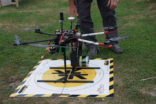
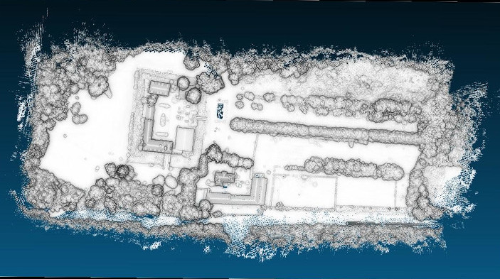
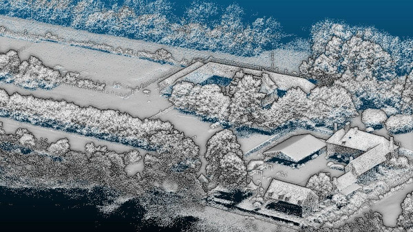
Figure 6: 3D Mapping process of the Manoir dataset. Top: map of the scanned area and scan device used for mapping. Bottom: two views of the resulting point cloud.

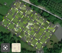
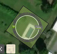
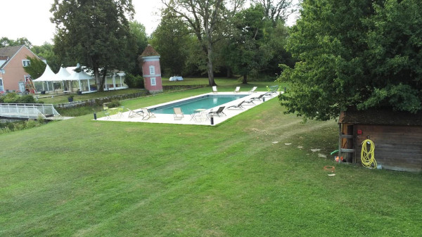
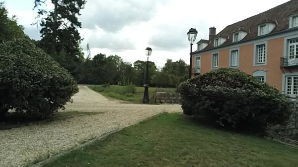
Figure 7: Video acquisition process of the Manoir dataset. Top: grid and orbit flight plan used for photogrammetry. Bottom: Video samples from the Anafi drone, 4k (left) and 720p (right)

5.2.2 Result

A subjective result of photogrammetry can be seen on Figure 8, for the optimal subset of 1000 frames and a full video taken by a drone. Finally, Figure 9 shows a sample of computed depth maps. A video playlist is available as a supplementary material for all the sequences

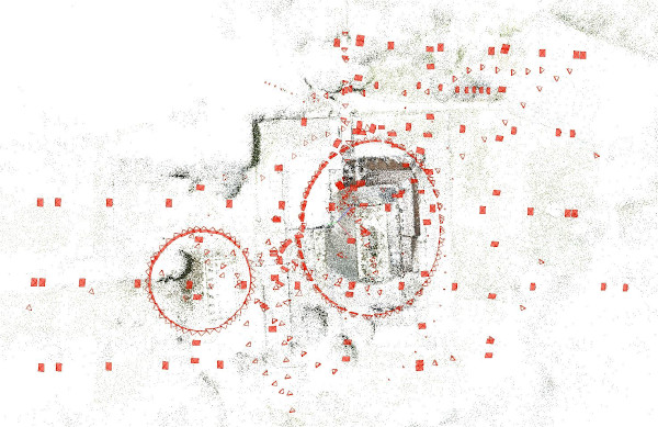
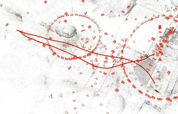
Figure 8: Left: global photogrammetry result (point cloud in black, camera odometry in red). Right: camera odometry during a given video footage (red curve), w.r.t. the global photogrammetry.

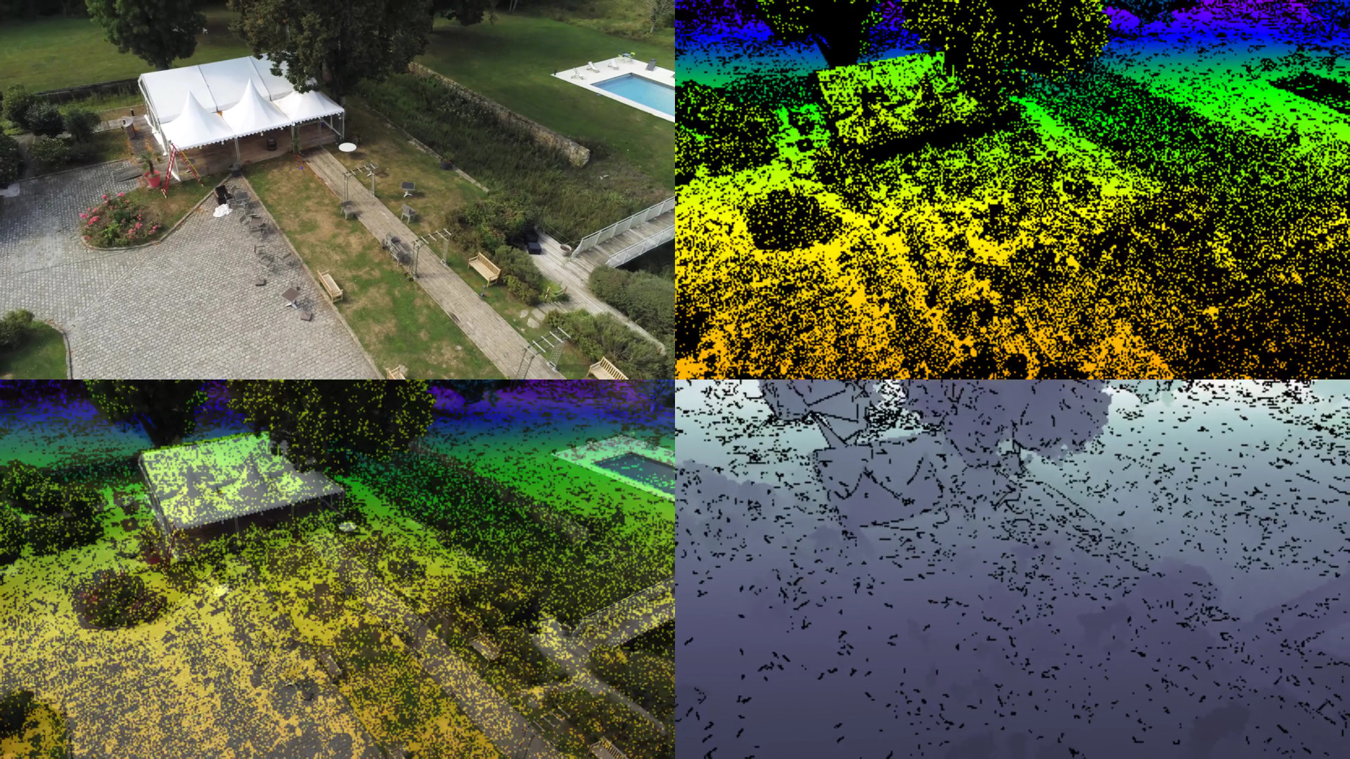
Figure 9: Depth result from the Manoir dataset. From left to right, top to bottom: RGB image, depth map, RGB + depth, occlusion depth.

5.2.3 Note on point cloud completeness

As it can be seen in Figure 6, the point cloud seriously lacks completeness for parts that are not easily seen from an altitude of 30 meters. This includes vertical sections like walls or poles, like seen in Figure 10, or cluttered sections, like under trees or inside a tunnel. From this remark, we can do two observations:

• Although it covers a large area very quickly, UAV Lidar scanning does not cover a wide range of viewpoints. The 30 meters altitude makes it difficult to see the same thing as within a few meters of altitude. As such, it would have been useful to add Lidar scans from a lower altitude, from other methods. For example, we can use fixed Lidar and handheld Lidar. Regarding this use case, we recommend to use a handheld Lidar because it’s much faster than fixed Lidar (typically as fast as human gait, while fixed Lidar requires several minutes per viewpoint), and if a UAV is available, all the hardware for using Lidar with IMU technique like e.g. LIO-SAM [32] or a proprietary technique like GeoSLAM is already available.

• In case no other Lidar scan is possible (e.g. because the area is not reachable other than with a drone), the COLMAP cloud is locally good. An interesting compromise for future work would be to combine the Lidar cloud with COLMAP reconstruction for obstacles very close to the camera.

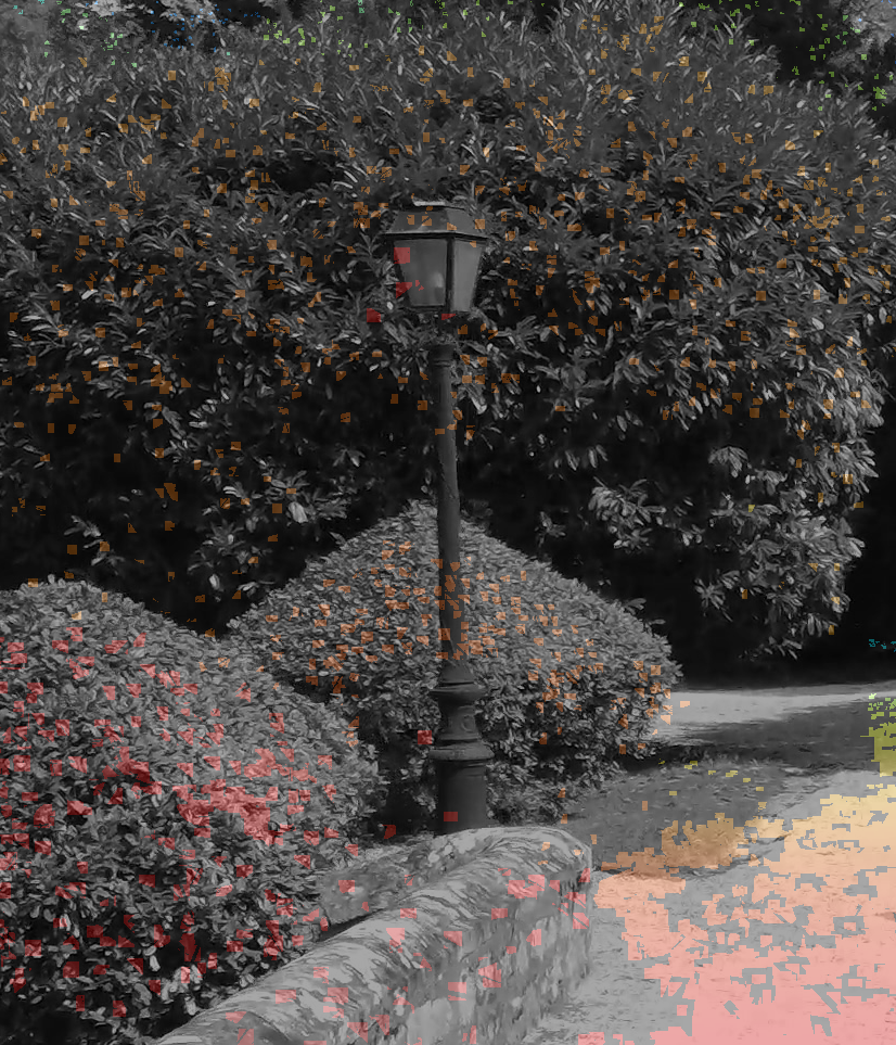
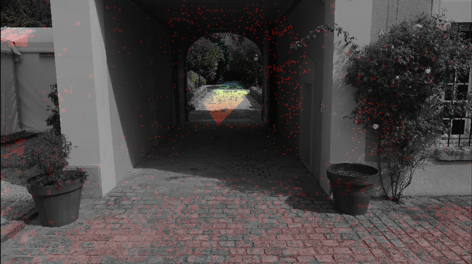
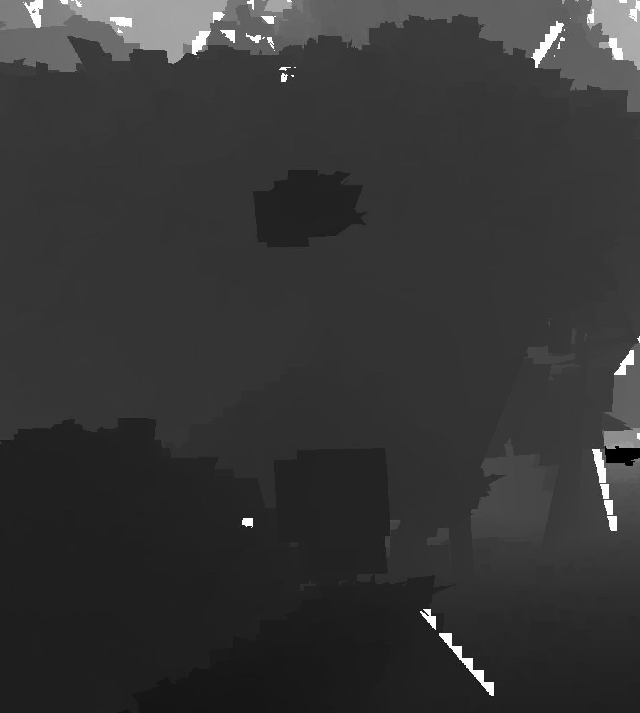
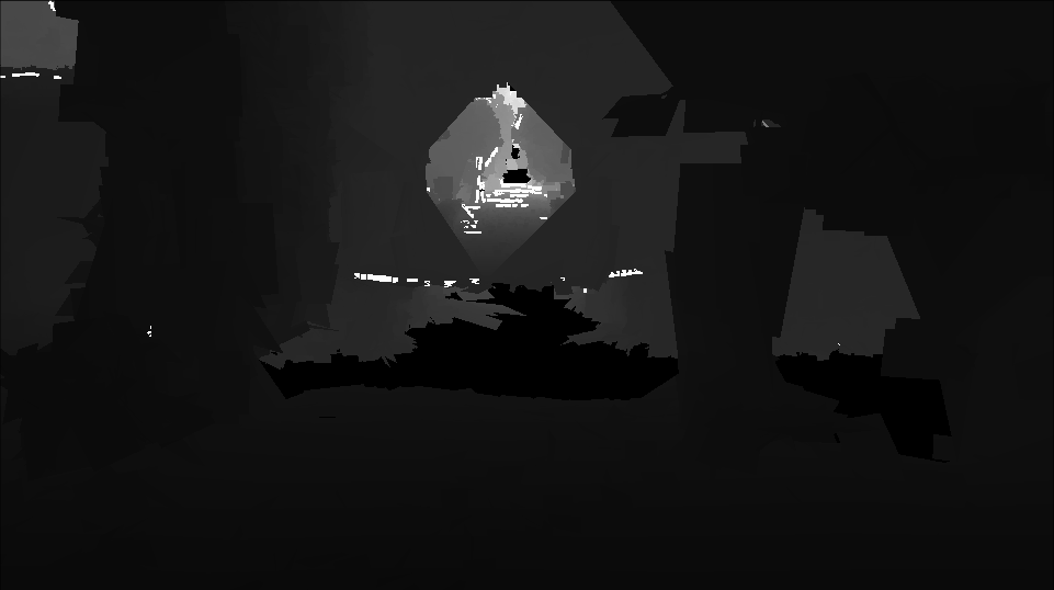
Figure 10: Images and corresponding occlusion depth maps illustrating problems coming from point cloud sparsity.

5.2.4 Benchmark

Scalar metrics are shown in Table 3. Distributions of (estimation / ground truth) ratios (equivalent to log depth difference, top), and log-errors according to the estimated depth (bottom) are shown on Figure 12 (left panel), while samples can be seen Figure 13 (first three rows). This first evaluation shows that unsurprisingly, DepthNet largely outperforms SFMLearner in all metrics. This is also visible on the log difference distribution: although both distributions have their maximum at a null log difference ( i.e. a ratio of 1), indicating an unbiased estimator, DepthNet’s distribution is much more concentrated. We can also see that both distribution exhibits a clear skewness toward negative difference. This is corroborated with the second plot where we can see that for both algorithms, the log error is much lower above 20 meters. This is a good hint for a potential drone manufacturer to think of a dedicated system for low depth values. For example, a stereo camera setup would be complementary to these two systems, because it’s more accurate for lower depth values.

For conciseness purpose, we have not shown all the histograms our tool can generate. However, we have made them easily generated within the tool we open sourced.

Method	MAE	MRE	MLE	SAE	SLE	$P_{1.25}$	$P_{1.25^{2}}$	$P_{1.25^{3}}$
SFMLearner [36]	18.40	0.5145	1.005	24.46	1.458	0.2395	0.4113	0.5385
DepthNet [24]	11.99	0.3275	0.5290	18.51	0.9099	0.5241	0.7069	0.7717

Table 3: Metric comparison between SFMLearner [36] and DepthNet [24] on Manoir dataset.

5.3 Second application: University hall dataset

5.3.1 Context

Our second use case is an indoor scene, shown on Figure 11, the hall of a University with a very high ceiling. For scan mapping, we use a handheld Zeb Horizon from GeoSLAM, with an announced precision of 4 cm. For videos, we used an Anafi; we have no photogrammetry-oriented frames. Like for Manoir dataset, the results of our small benchmark can be seen on Table 4 and Figure 12 (right panel). Some samples can be seen Figure 13 (last two rows)

Although DepthNet still outperforms SFMLearner for most metrics, the estimation accuracy is much lower. This can be explained by the fact that the university hall is mostly composed of completely white walls, with many glass windows and a somewhat reflective ground. This is a very challenging use case for SFM based training and inference methods. These results indicate that both SFMLearner and DepthNet are much more suited for outdoor scenarios, with irregular textured surfaces, and that active sensing solutions like structured light or time-of-flight are probably more interesting for this dataset.

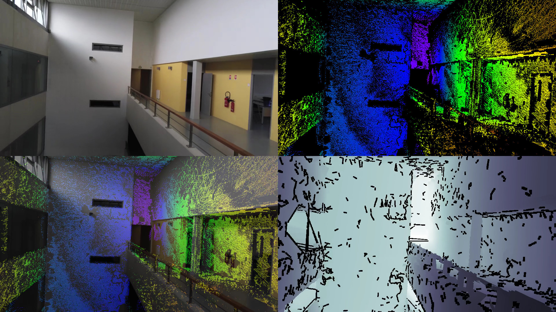
Figure 11: University hall depth visualization, same structure as Figure 9

Method	MAE	MRE	MLE	SAE	SLE	$P_{1.25}$	$P_{1.25^{2}}$	$P_{1.25^{3}}$
SFMLearner [36]	10.25	1.0225	0.5682	18.29	0.7798	0.3180	0.5461	0.6912
DepthNet [24]	5.890	0.5197	0.5056	10.612	0.726	0.3184	0.5982	0.7694

Table 4: Metric comparison between SFMLearner [36] and DepthNet [24] on University hall dataset

Figure 12: Comparison of error distributions between SFMLearner [36] and DepthNet [24] on Manoir dataset (left) and on University hall dataset (right) Top: Distribution of ratios between estimation and ground truth (above 1 means estimation is higher), at log scale. This is equivalent to the log difference distribution. Bottom: Log error as a function of estimated depth. For visualization purpose, the $y$ scale is logarithmic. The curve shows the median value and the shaded area represents the $50\%$ confidence interval.

Image	GroudTruth	DepthNet[23]	SFMLearner [36]

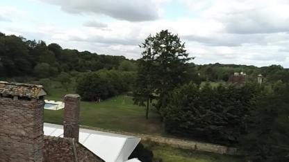
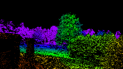
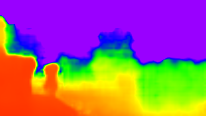
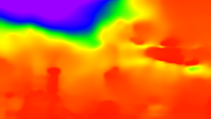
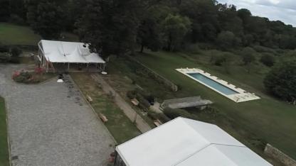
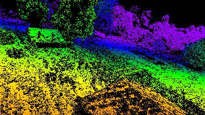
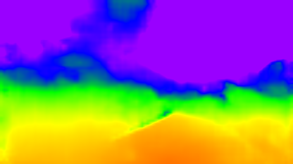
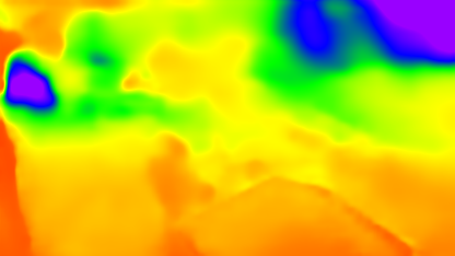
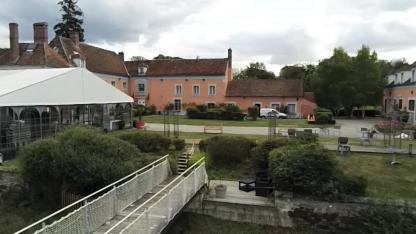
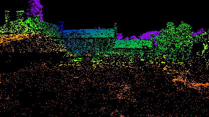
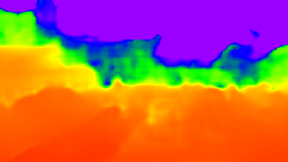
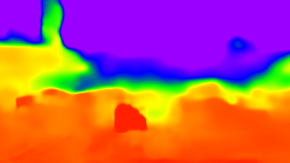
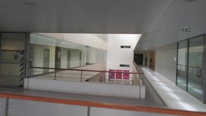
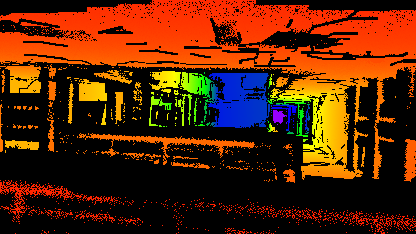
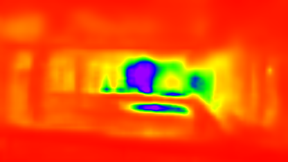
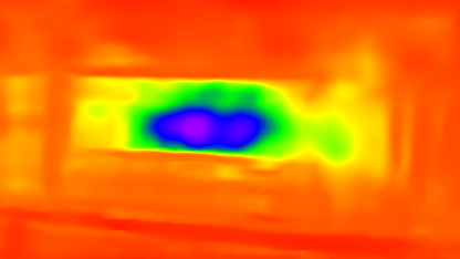
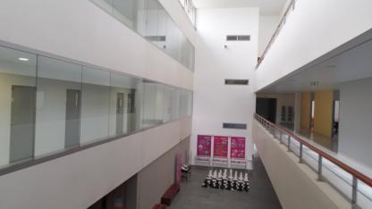
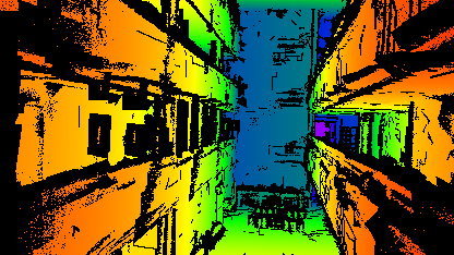
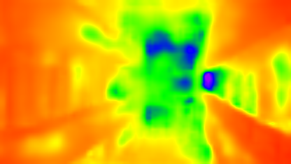
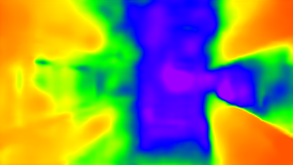
Figure 13: Vizualisation of some samples on Manoir and University hall data sets. Colormap is OpenCV Rainbow, normalized to Ground truth.

6 Discussion and conclusive remarks

In this paper, we presented RDC, a powerful tool for depth dataset generation. It is very flexible with respect to available budget and hardware. Its context of application can be as rudimentary as no-budget-at-all, only using a handheld camera (e.g. the user’s phone camera), and still it lets a user make the most of limited means, to have depth enabled videos with potentially infinite range. By leaving open access to future users, we hope to improve it by gradually increasing the diversity of use cases.

6.1 Limitations

RDC still suffers from some already known limitations:

• The first limitation is obviously the need for a rigid scene. Although this problem can be mitigated in the case of a UAV flying, it can be particularly problematic for in-car environment in a urban area where many people and other vehicles are dynamic. It can also be a problem when Lidar scanning and video recording are not done at the same time, in a scene with rigid but movable objects. This was the case in the University hall dataset, where some seats had been moved, thus making some depth maps useless. A possible solution would be to combine a dense high quality point cloud of a scene, scanned beforehand, and sparse point cloud from a mobile Lidar. By characterizing possible dynamic elements, like humans and other vehicles in a urban area, we may be able to discard the depth map from rigid scene where the dynamic elements are segmented, and replace it with the depth from the sparse mobile Lidar.

• Although it does not require heavy hardware for data acquisition, the computer used by this tool must be powerful (as with any photogrammetry task), and have plenty of disk space, which mitigates the fact that we adapt to any kind of budget. However, a regular gaming desktop computer is often enough, and is orders of magnitude cheaper than a full Lidar and cam rig solution.

• Although it can be improved by using better registration algorithms than a simple ICP, the registration part will often need a human eye to assess the registration quality. This part of the process lies in the middle of it, which makes the tool not totally automatic. It is essential that it happens after the photogrammetry and before ground truth generation, so there is no obvious solution yet.

• When the camera is located in a very sparse portion of the point cloud, the occlusion depth will be of poor quality. It is possible that the end user will discover after the whole dataset creation process that some scenes would need a better scanning process. It would then be interesting to enter a warning before the end of the process, as soon as the Lidar point cloud is registered, that some areas lack data.

6.2 Further work

The next logical step is now to construct a more comprehensive dataset with this tool, using different scenes, contexts, and modalities, in the same way ETH3D dataset was built, but with much more frames.

Additionally, a full evaluation suite would be very beneficial, as this initial version only provides basic examples of histogram based algorithm quality assessment.

Finally, now that we have a way of localizing video frames in a point cloud, we can make more ground truths to test other kinds of algorithms:

• From odometry and ground truth point cloud, ground truth optical flow can be deduced.

• If we annotate the Lidar point cloud with semantic parts, we can construct semantic segmentation maps.

References

- [1] P. J. Besl and N. D. McKay. A method for registration of 3-d shapes. IEEE Transactions on Pattern Analysis and Machine Intelligence, 14(2):239–256, 1992.
- [2] D. J. Butler, J. Wulff, G. B. Stanley, and M. J. Black. A naturalistic open source movie for optical flow evaluation. In A. Fitzgibbon et al. (Eds.), editor, European Conf. on Computer Vision (ECCV), Part IV, LNCS 7577, pages 611–625. Springer-Verlag, Oct. 2012.
- [3] Yang Chen and Gerard Medioni. Object modelling by registration of multiple range images. Image and Vision Computing, 10(3):145 – 155, 1992. Range Image Understanding.
- [4] A. Dosovitskiy, P. Fischer, E. Ilg, P. Häusser, C. Hazırbaş, V. Golkov, P. v.d. Smagt, D. Cremers, and T. Brox. Flownet: Learning optical flow with convolutional networks. In IEEE International Conference on Computer Vision (ICCV), 2015.
- [5] David Eigen, Christian Puhrsch, and Rob Fergus. Depth map prediction from a single image using a multi-scale deep network. Advances in neural information processing systems, 27:2366–2374, 2014.
- [6] Huan Fu, Mingming Gong, Chaohui Wang, Kayhan Batmanghelich, and Dacheng Tao. Deep Ordinal Regression Network for Monocular Depth Estimation. In IEEE Conference on Computer Vision and Pattern Recognition (CVPR), 2018.
- [7] Ravi Garg, BG Vijay Kumar, Gustavo Carneiro, and Ian Reid. Unsupervised cnn for single view depth estimation: Geometry to the rescue. In European Conference on Computer Vision, pages 740–756. Springer, 2016.
- [8] Andreas Geiger, Philip Lenz, and Raquel Urtasun. Are we ready for autonomous driving? the kitti vision benchmark suite. In 2012 IEEE Conference on Computer Vision and Pattern Recognition, pages 3354–3361. IEEE, 2012.
- [9] Clément Godard, Oisin Mac Aodha, Michael Firman, and Gabriel J. Brostow. Digging into self-supervised monocular depth prediction. In The International Conference on Computer Vision (ICCV), October 2019.
- [10] Ariel Gordon, Hanhan Li, Rico Jonschkowski, and Anelia Angelova. Depth from videos in the wild: Unsupervised monocular depth learning from unknown cameras. In Proceedings of the IEEE/CVF International Conference on Computer Vision (ICCV), October 2019.
- [11] Richard Hartley and Andrew Zisserman. Multiple View Geometry in Computer Vision. Cambridge University Press, 2 edition, 2004.
- [12] Michael Kazhdan, Matthew Bolitho, and Hugues Hoppe. Poisson surface reconstruction. In Proceedings of the fourth Eurographics symposium on Geometry processing, volume 7, 2006.
- [13] Arno Knapitsch, Jaesik Park, Qian-Yi Zhou, and Vladlen Koltun. Tanks and temples: Benchmarking large-scale scene reconstruction. ACM Transactions on Graphics, 36(4), 2017.
- [14] Karl Kraus, Ian A. Harley, and Stephen Kyle. Photogrammetry: Geometry from Images and Laser Scans. De Gruyter, Berlin, Boston, 18 Oct. 2011.
- [15] Matej Kristan, Jiri Matas, Aleš Leonardis, Tomas Vojir, Roman Pflugfelder, Gustavo Fernandez, Georg Nebehay, Fatih Porikli, and Luka Čehovin. A novel performance evaluation methodology for single-target trackers. IEEE Transactions on Pattern Analysis and Machine Intelligence, 38(11):2137–2155, Nov 2016.
- [16] P. Labatut, J.-P. Pons, and R. Keriven. Robust and Efficient Surface Reconstruction From Range Data. Computer Graphics Forum, 2009.
- [17] Jin Han Lee, Myung-Kyu Han, Dong Wook Ko, and Il Hong Suh. From big to small: Multi-scale local planar guidance for monocular depth estimation. arXiv preprint arXiv:1907.10326, 2019.
- [18] Brett T Lopez and Jonathan P How. Aggressive 3-d collision avoidance for high-speed navigation. In 2017 IEEE International Conference on Robotics and Automation (ICRA), pages 5759–5765. IEEE, 2017.
- [19] J. Macqueen. Some methods for classification and analysis of multivariate observations. In In 5-th Berkeley Symposium on Mathematical Statistics and Probability, pages 281–297, 1967.
- [20] Lazaros Nalpantidis, Ioannis Kostavelis, and Antonios Gasteratos. Stereovision-based algorithm for obstacle avoidance. In International Conference on Intelligent Robotics and Applications, pages 195–204. Springer, 2009.
- [21] Pushmeet Kohli Nathan Silberman, Derek Hoiem and Rob Fergus. Indoor segmentation and support inference from rgbd images. In ECCV, 2012.
- [22] Clément Pinard. Robust Learning of a depth map for obstacle avoidance with a monocular stabilized flying camera. Theses, Université Paris Saclay (COmUE), June 2019.
- [23] C. Pinard, L. Chevalley, A. Manzanera, and D. Filliat. End-to-end depth from motion with stabilized monocular videos. ISPRS Annals of Photogrammetry, Remote Sensing and Spatial Information Sciences, IV-2/W3:67–74, 2017.
- [24] Clément Pinard, Laure Chevalley, Antoine Manzanera, and David Filliat. Learning structure-from-motion from motion. In Proceedings of the European Conference on Computer Vision (ECCV), 2018.
- [25] Abraham. Savitzky and M. J. E. Golay. Smoothing and differentiation of data by simplified least squares procedures. Analytical Chemistry, 36(8):1627–1639, 1964.
- [26] Ashutosh Saxena, Sung H Chung, and Andrew Y Ng. 3-d depth reconstruction from a single still image. International journal of computer vision, 76(1):53–69, 2008.
- [27] Hendrik Schilling, Marcel Gutsche, Alexander Brock, Dane Späth, Carsten Rother, and Karsten Krispin. Mind the gap - a benchmark for dense depth prediction beyond lidar. In 2020 IEEE Conference on Computer Vision and Pattern Recognition Workshops (CVPRW), volume in press, 2020.
- [28] Johannes Lutz Schönberger and Jan-Michael Frahm. Structure-from-motion revisited. In Conference on Computer Vision and Pattern Recognition (CVPR), 2016.
- [29] Johannes Lutz Schönberger, True Price, Torsten Sattler, Jan-Michael Frahm, and Marc Pollefeys. A vote-and-verify strategy for fast spatial verification in image retrieval. In Asian Conference on Computer Vision (ACCV), 2016.
- [30] Johannes Lutz Schönberger, Enliang Zheng, Marc Pollefeys, and Jan-Michael Frahm. Pixelwise view selection for unstructured multi-view stereo. In European Conference on Computer Vision (ECCV), 2016.
- [31] Thomas Schöps, Johannes L. Schönberger, Silvano Galliani, Torsten Sattler, Konrad Schindler, Marc Pollefeys, and Andreas Geiger. A multi-view stereo benchmark with high-resolution images and multi-camera videos. In Conference on Computer Vision and Pattern Recognition (CVPR), 2017.
- [32] Tixiao Shan, Brendan Englot, Drew Meyers, Wei Wang, Carlo Ratti, and Rus Daniela. Lio-sam: Tightly-coupled lidar inertial odometry via smoothing and mapping. In IEEE/RSJ International Conference on Intelligent Robots and Systems (IROS), pages 5135–5142. IEEE, 2020.
- [33] G. K. L. Tam, Z. Cheng, Y. Lai, F. C. Langbein, Y. Liu, D. Marshall, R. R. Martin, X. Sun, and P. L. Rosin. Registration of 3d point clouds and meshes: A survey from rigid to nonrigid. IEEE Transactions on Visualization and Computer Graphics, 19(7):1199–1217, 2013.
- [34] Jonas Uhrig, Nick Schneider, Lukas Schneider, Uwe Franke, Thomas Brox, and Andreas Geiger. Sparsity invariant cnns. In International Conference on 3D Vision (3DV), 2017.
- [35] Igor Vasiljevic, Nick Kolkin, Shanyi Zhang, Ruotian Luo, Haochen Wang, Falcon Z. Dai, Andrea F. Daniele, Mohammadreza Mostajabi, Steven Basart, Matthew R. Walter, and Gregory Shakhnarovich. DIODE: A Dense Indoor and Outdoor DEpth Dataset. CoRR, abs/1908.00463, 2019.
- [36] Tinghui Zhou, Matthew Brown, Noah Snavely, and David G. Lowe. Unsupervised learning of depth and ego-motion from video. In CVPR, 2017.