Joint Resource Allocation and Transceiver Design for Sum-Rate Maximization under Latency Constraints in Multicell MU-MIMO Systems

Abstract

Due to the continuous advancements of orthogonal frequency division multiplexing (OFDM) and multiple antenna techniques, multiuser multiple input multiple output (MU-MIMO) OFDM is a key enabler of both fourth and fifth generation networks. In this paper, we consider the problem of weighted sum-rate maximization under latency constraints in finite buffer multicell MU-MIMO OFDM systems. Unlike previous works, the optimization variables include the transceiver beamforming vectors, the scheduled packet size and the resources in the frequency and power domains. This problem is motivated by the observation that multicell MU-MIMO OFDM systems serve multiple quality of service classes and the system performance depends critically on both the transceiver design and the scheduling algorithm. Since this problem is non-convex, we resort to the max-plus queuing method and successive convex approximation. We propose both centralized and decentralized solutions, in which practical design aspects, such as signaling overhead, are considered. Finally, we compare the proposed framework with state-of-the-art algorithms in relevant scenarios, assuming a realistic channel model with space, frequency and time correlations. Numerical results indicate that our design provides significant gains over designs based on the wide-spread saturated buffers assumption, while also outperforming algorithms that consider a finite-buffer model.

I Introduction

Driven by the insatiable demands for mobile broadband and low-delay services, the fourth and fifth generations of cellular networks have been advancing in terms of capacity, spectral efficiency, reliability and latency. Indeed, the rapidly increasing number of mobile data subscriptions along with a continuous increase in the average data volume per subscription has been leading to a compounded annual growth rate in world-wide data traffic from 8.8 exabytes to above 70 exabytes between 2016 to 2022 [1].

In this context, current wireless systems do not only have to cope with the growing number of data-hungry applications, but also with a large number of devices connected to the network. In addition, new use cases, such as intelligent transport systems, industrial automation, augmented reality and e-health, impose strict requirements in terms of latency and link reliability, thus demanding sophisticated methods that are able to fulfill these diverse system demands [2, 3]. In particular, it is crucial to develop methods that are able to optimize spectrum utilization considering QoS constraints.

Due to the continuous advancements of OFDM and multiple antenna techniques, MU-MIMO OFDM has become a key enabler of both fourth and fifth generation (4G/5G) networks. Indeed, MU-MIMO systems have the potential to increase the spectral efficiency by allowing multiple independent data streams on shared frequency [4] while OFDM has low-complexity transceiver design, high spectral efficiency, and easy integration with MIMO technologies [5].

In general, in MU-MIMO OFDM systems, binary decision variables are often advantageously used for frequency-time resource assignment, which consists in indicating when a given user is assigned to a particular resource [6]. Nevertheless, since linear transmit beamformers are complex vectors, the decision variables can be implicitly modeled by them, which avoids binary decision variables. In fact, once the design stage is done, the zero transmit beamforming vector indicates that a user is not assigned on a given resource, whereas the non-zero transmit beamforming vectors are used to determine the transmission rates of users on a space-frequency resource.

In addition, the performance of MU-MIMO OFDM systems significantly depends on the considered traffic model. In this context, two models have been adopted in the recent literature: full-buffer and finite-buffer [7]. On the one hand, the full-buffer traffic model is characterized by having an unlimited amount of data to transmit in the users’ buffers. Moreover, due to the absence of the packets’ arrival process, the number of users in the system is constant. The main advantage of this model is its simplicity, thus it has been widely adopted for theoretical investigations [8, 9]. On the other hand, the finite-buffer model assumes a finite amount of data to be transmitted or received in the users’ buffers. Moreover, both packets arrival and departure processes are considered, which leads to a variation in the number of users in the system. In other works, a given user is assigned a finite payload upon arrival, leaving the system after the payload transmission or reception is completed. Even though this model has been less adopted than the full-buffer model, it should be more appropriate for practical scenarios [7].

II Related Works and Main Contributions

Recognizing the importance of resource allocation in multi-antenna systems, the research community has proposed various resource allocation schemes that are applicable specifically in multi-antenna systems. We categorize these schemes in terms of the number of sub-channels and whether they are applicable in full-buffer or finite buffer systems. Following this literature review, we specify the contribution of the present paper to this line of research.

II-A Resource Allocation in Multi-Antenna Systems with a Single Sub-Channel and Full-Buffer Traffic

In the literature, transceiver design has often been studied in the form of optimization problems with different objectives and constraints, as seen in [10] and references therein. Among the possible objectives, sum-rate maximization is a well-motivated and often pursued problem formulation. In [11] the authors studied the sum-rate maximization problem in multicell MISO systems, presenting a solution based on the BB method. In [12] and [13], the authors proposed centralized and distributed solutions by exploiting an iterative WMMSE approach for a single-cell and multicell MU-MIMO systems, respectively. Such a scenario was studied in [14], for which a centralized iterative algorithm based on fractional programming was proposed. In [15] the authors also proposed a centralized solution based on geometric programming. An algorithm based on matrix fractional programming was proposed in [16], where the authors proved the convergence of their algorithm using the minorization-maximization approach.

Although these works focused on the weighted sum-rate problem, the scheduling aspect focusing on guaranteeing some per-user minimum QoS was not considered. In the literature, QoS aspects have been extensively considered in the context of sum-power minimization, such as those in [17, 18, 19]. In [17] the sum-power minimization problem subject to SINR constraints was studied and a centralized solution based on MMSE and uplink-downlink duality was proposed. In addition, a rigorous convergence analysis was also provided. Centralized and distributed algorithms for sum-power minimization under minimum SINR constrains were also proposed in [19] and [18]. Other works, such as [20, 21], have focused on the sum-energy efficiency maximization problem, that consists in minimizing the energy consumption per transmitted bit. The weighted sum-rate maximization problem with QoS guarantees was considered in [22, 23, 24]. In [22] the authors proposed centralized and distributed solutions based on SCA, DCP and Lagrangian relaxation. Centralized, semi-distributed and distributed solutions were proposed in [23, 24] based on the BB method, geometric programming and SOCP, SCA and DCP.

II-B Resource Allocation in Multi-Antenna Systems with Multiple Sub-Channels and Full-Buffer Traffic

Although the works listed in the previous subsection consider some minimum QoS assurance, they assume a predetermined frequency-time resource assignment. Therefore, the full potential of transceiver design and MU-MIMO OFDM systems is still not fully explored. In the literature, frequency-time resource assignment with QoS guarantees in MU-MIMO single-cell systems was studied in [25, 26, 27]. In [25], the authors proposed a low-complexity frequency-time resource allocation algorithm for the sum-power minimization problem under rate constraints. Fairness aspects were considered for MU-MIMO OFDM in [26] by using nonlinear DPC-based techniques. However, the DPC technique makes the proposed solution computationally complex, which is not desirable for practical implementations of real-time networks where complexity is an important feature. In [28] the sum-rate maximization problem with frequency-time resource assignment was considered in multi-service scenarios. However, the joint space-frequency resource allocation was ignored in [28], which was considered in another work by the same authors in [27]. Nevertheless, they also assume the use of linear transmit beamformers with equal power allocation, consequently, they do not perform precoder optimization. A joint transceiver design and space-frequency resource allocation in a multicell scenario was considered in [6] and [29]. In [6] the authors studied the sum-power minimization problem with SINR constraints, where a centralized solution based on a BB algorithm was proposed. In [29], on the other hand, the weighted sum-rate problem was considered but the QoS aspects were ignored. Moreover, decentralized solutions were not proposed in [6] and [29].

II-C Resource Allocation in Multi-Antenna Systems with Finite-Buffer Traffic

The works listed in the previous subsections have addressed QoS aspects and joint space-frequency resource allocation. However, they assumed a full-buffer model in their modeling. As previously mentioned, these solutions cannot achieve the desired performance in practical scenarios where the finite-buffer model is more suitable. In [30] the finite-buffer model was considered and the queue minimization problem was studied using geometric programming. In [31] the authors used the max-plus queuing approach for establishing a suitable model to characterize packet latency and then transform the latency outage probability requirements into minimum data rate constraints. However, these works assumed single antenna transmitters and receivers, which reduces their problems to power allocation problems. In [32] the weighted sum-rate problem was studied assuming a finite-buffer model for single-cell MISO scenarios. In [33] the authors proposed a distributed solution based on Lyapunov optimization for energy-efficiency with time average QoS constraints in a multicell MISO scenario. Centralized and distributed solutions were proposed in [34] for maximizing the overall system utility while stabilizing all transmission queues in multicell MU-MIMO scenarios. Nevertheless, [32, 33, 34] consider a single sub-channel, thus not exploiting the full potential of OFDM. The problem of transceiver design and resource allocation over the space-frequency resources without binary decision variables provided by MU-MIMO OFDM was studied in [35], where the authors proposed centralized and distributed solutions based on SCA and alternating optimization for minimizing the number of backlogged packets waiting at each BS. In addition, in [36] the same authors extended the framework proposed in [35] in order to reduce the signaling overhead, employing bidirectional training based on over-the-air signaling to update the coupling inter-cell interference variables. However, both [35] and [36] ignored per-user QoS aspects. In [37] the authors considered the latency outage probability requirement, while minimizing BS usage and reducing the interfering range in distributed MIMO cooperative systems. In [38] the weighted sum-rate maximization problem subject to latency outage probability requirements was studied in a single-cell MU-MIMO scenario. However, by increasing the number of cells, a more complex structure of the transceiver must be designed to combat the multicell interference, and the centralized scheme developed in [38] becomes impractical in such scenarios.

II-D Main Contributions

The main contributions of this work are summarized as:

1. Investigation of a variant of the weighted sum-rate maximization problem in which we introduce latency outage probability constraints for multicell MU-MIMO OFDM systems with finite-buffer. Therefore, the formulated problem considers altogether the transceiver design in MIMO systems, user scheduling across multiple sub-channels, minimum QoS requirements and a finite-buffer traffic model.

2. Development of a centralized solution based on SCA, which is employed to handle the non-convexity of the formulated optimization problem. Moreover, a novel decentralized solution based on a partial Lagrangian relaxation and a subsequent primal-dual method is also provided, for which we present a signaling scheme for deployments in practical multicell MU-MIMO OFDM systems. The decentralized algorithm is highly non-trivial due to the inherent coupling between the BSs.

3. A convergence analysis is provided proving that both centralized and decentralized solutions converge to a KKT point of the novel formulated problem. Our converge analysis is based on [22].

4. Performance evaluation by means of simulations, where we compare the proposed solution with state-of-the-art optimization-based algorithms considering different aspects, including Poisson and bursty traffic models, as well as imperfect CSI. Unlike previous works, we consider a realistic channel modeling based on the 3GPP’s stochastic channel model with spatial, frequency and time correlations. Simulations show that the proposed solution efficiently handles the resource allocation across multiple sub-channels and finite-buffer scheduling, while presenting performance gains in terms of outage probability and latency.

Organization: The remainder of the paper is organized as follows. Sections III and IV introduce the system model and the weighted sum-rate maximization problem with maximum outage probability constraints, respectively. Section V describes the proposed centralized solution. Section VI presents the proposed decentralized solution along with the involved signaling aspects. Section VII provides the numerical results along with discussions and, finally, Section VIII highlights the main conclusions, as well as perspectives for future works.

Notation: Throughout the paper, matrices and vectors are presented by boldface upper and lower case letters, respectively. $\mathbf{X}^{T}$, $\mathbf{X}^{H}$, $\mathbf{X}^{-1}$ and $\mathbf{X}^{\dagger}$ stand, respectively, for transpose, Hermitian, inverse and pseudo-inverse of a matrix $\mathbf{X}$. $\{x_{i}\}_{\forall i}$ denotes the set of elements $x_{i}$ for the values of $i$ denoted by the subscript expression. $\mathbf{I}$ is the identity matrix. Mapping of negative scalars to zero is written as $(\cdot)^{+}=\text{max}(0,\cdot)$. Expected value of a random variable is denoted by $\mathbb{E}[\cdot]$. For a matrix $\mathbf{X}$, $\operatorname{tr}\left(\mathbf{X}\right)$ and $\det(\mathbf{X})$ are the trace and determinant operators, respectively.

III System Model

We consider the downlink of a multicell MU-MIMO scenario in an OFDM framework composed of $N$ sub-channels, where $B$ BS equipped with $N_{\text{T}}$ antennas serve a total of $U$ multi-antenna UE, each one equipped with $N_{\text{R}}$ antennas. Let $\mathcal{U}=\{1,2,\ldots,U\}$ indicate the set of all users in the system. The number of users associated with BS $b$ is denoted by $U_{b}$, where each user $u$ is served by a single BS $b_{u}$. We assume that all BS serve the respective users with linear transmit beamforming.

We let $S$ denote the maximum number of spatial streams. The downlink signal received by user $u$ on sub-channel $n$ is given by

$$\mathbf{y}_{u,n}=\;\mathbf{H}_{b_{u},u,n}\mathbf{M}_{u,n}\mathbf{x}_{u,n}+\sum_{\begin{subarray}{c}i=1\\ i\neq u\end{subarray}}^{U}\mathbf{H}_{b_{i},u,n}\mathbf{M}_{i,n}\mathbf{x}_{i,n}+\mathbf{n}_{u,n},$$ (1)

where $\textbf{H}_{b_{i},u,n}\in\mathbb{C}^{N_{\text{R}}\times N_{\text{T}}}$ is the channel matrix between user $u$ and BS $b$ serving user $i$ on sub-channel $n$, $\mathbf{M}_{u,n}\in\mathbb{C}^{N_{\text{T}}\times S}$ is the transmit beamforming matrix that the BS uses on sub-channel $n$ to transmit the symbol $\mathbf{x}_{u}\in\mathbb{C}^{S\times 1}$ to user $u$ with ${\mathbb{E}\left[\mathbf{x}_{u}{\mathbf{x}}^{\mathrm{H}}_{u}\right]=\mathbf{I}}$ and $\textbf{n}_{u,n}\in\mathbb{C}^{N_{\text{R}}}\sim\mathcal{C}\mathcal{N}(0,\sigma^{2})$ is the noise at user ${u}$ and sub-channel $n$. User $u$ decodes the signal $\textbf{y}_{u,n}$ via a receive beamformer matrix $\mathbf{W}_{u,n}\in\mathbb{C}^{N_{\text{R}}\times S}$ so that the estimated symbol is given by

$$\hat{\mathbf{x}}_{u,n}={\mathbf{W}}^{\mathrm{H}}_{u,n}\mathbf{y}_{u,n}.$$ (2)

Furthermore, the rate assigned to user $u$ is $r_{u}=\sum\limits_{n=1}^{N}r_{u,n}$, where $r_{u,n}$ is the number of transmitted bits per second for user $u$ on sub-channel $n$, which is given by

$$r_{u,n}=\log_{2}\det\left(\mathbf{I}+\mathbf{H}_{b_{u},u,n}\mathbf{M}_{u,n}{\mathbf{M}}^{\mathrm{H}}_{u,n}{\mathbf{H}}^{\mathrm{H}}_{b_{u},u,n}\left(\sum_{\begin{subarray}{c}i=1\\ i\neq u\end{subarray}}^{U}\mathbf{H}_{b_{i},u,n}\mathbf{M}_{i,n}{\mathbf{M}}^{\mathrm{H}}_{i,n}{\mathbf{H}}^{\mathrm{H}}_{b_{i},u,n}+\sigma^{2}\mathbf{I}\right)^{-1}\right).$$ (3)

We assume the availability of perfect CSI at the transmitters and receivers for the design of the proposed algorithms, similarly to the assumptions used in [13, 12, 22, 19]. In other words, we assume that the channel matrix is perfectly known at transmitters and receivers without channel estimation errors. Moreover, we consider that the channel matrices are generated using a realistic channel modeling based on the 3GPP’s stochastic channel model with spatial, frequency and time correlations [39, 40].

It is assumed that the packet arrival process for the $u$-th user is independent and identically distributed (i.i.d) over the time slots and follows a Poisson distribution with average arrival rate $\lambda_{u}$ [35, 31]. Also, the $m$-th packet size for user $u$, denoted by $L_{u,m}$, is i.i.d over the time slots and follows an exponential distribution with mean packet size $\overline{L}_{u,m}$. We let $Q_{u}$ represent the number of backlogged packets destined for user $u$. The waiting time of the $m$-th packet in the buffer of user $u$ is given by $W_{u,m}$ and the respective transmission time is $\delta_{u,m}$. Therefore, the latency of the $m$-th packet destined to user $u$ is written as

$$D_{u,m}=W_{u,m}+\delta_{u,m},$$ (4)

which is given in time slots. Let us denote the maximum tolerable latency for packet transmission as $d_{\text{max}}$ (in time slots) and the maximum outage probability as $\xi$. Thus, the latency outage probably requirement of user $u$ can be expressed as

$$P\{D_{u,m}>d_{\text{max}}\}\leq\xi.$$ (5)

IV Problem Formulation

We consider the following variant of the transceiver design problem for weighted sum-rate maximization in MU-MIMO OFDM systems under per-BS maximum power and per-user latency constraints:

$$\underset{\mathbf{W}_{u,n},\mathbf{M}_{u,n}}{\text{maximize}} \quad\sum\limits_{u=1}^{U}\beta_{u}\sum_{n=1}^{N}r_{u,n}$$ (6a)

subject to $$\quad\sum\limits_{u=1}^{U_{b}}\sum\limits_{n=1}^{N}\operatorname{tr}\left(\mathbf{M}_{u,n}{\mathbf{M}}^{\mathrm{H}}_{u,n}\right)\leq P_{b}, \forall b,$$ (6b)

$$\quad P\{D_{u,m}>d_{\text{max}}\}\leq\xi, \forall u,m,$$ (6c)

$$\quad\sum_{n=1}^{N}r_{u,n}\leq\frac{Q_{u}}{\Delta_{\text{TTI}}}, \forall u,$$ (6d)

where $\beta_{u}>0$ denotes the priority weight of user $u$, $P_{b}$ denotes the power budget of BS $b$ and $\Delta_{\text{TTI}}$ is the duration of one TTI. The optimization variables are the transmit and receive beamforming matrices $\mathbf{M}_{u,n}\in\mathbb{C}^{N_{\text{T}}\times S}$ and $\mathbf{W}_{u,n}\in\mathbb{C}^{N_{\text{R}}\times S}$ $\forall(u,n)$, respectively. Observe that constraints (6c) implicitly depend on the optimization variables. In fact, the higher is the rate allocated to user $u$, the faster the $m$-th packet destined to user $u$ will be transmitted from the BS to user $u$. Since the rate allocated to user $u$ depends on the transmit beamformers $\{\mathbf{M}_{u,n}\}_{\forall(n)}$ and on the receive beamformers $\{\mathbf{W}_{u,n}\}_{\forall(n)}$ computed for that user, consequently, both transmit and receive beamforming have an impact on the outage probability requirement of user $u$. Finally, constraints (6d) state that the sum of the bits transmitted to user $u$ cannot be higher than the amount of bits in its buffer in order to avoid excessive allocation of the resources. Unlike the full-buffer model, in which the transmit buffers relative to the users always have an unlimited amount of data to be transmitted, the finite-buffer model assumes that such buffers have a limited amount of data. Thus, the maximum allowed user rate can also be determined by the users’ transmit buffer located at the BS. Recognizing this, and in order to arrive at industrially applicable results, we are motivated to explicitly incorporate the finite buffer in our model, whose size is a system parameter. The importance of these additional constraints will be clearly shown by means of simulations in Section VII.

Therefore, the formulated problem allows to simultaneously optimize the transceiver design and schedule the users across space-frequency resources in order to satisfy their packet latency and rate demands, while also handling more realistic finite-buffer traffic models. However, the packet latency as defined in (4) is very difficult to compute directly, thus the latency constraints (6c) require some transformation so that we arrive at a tractable form. Besides that, we remark that the sum-rate maximization problem considering an interference channel (i.e., with only one user per BS) was shown to be strongly NP-hard in Theorem 1 and Theorem 6 of [44]. In fact, this NP-hardness was demonstrated in [44] even for a very simple case (considering only one sub-channel and optimizing only the powers at the BS). The sum-rate maximization considered in our case, i.e., problem (6), has clearly a wider set of feasible solutions, since it involves transceiver designs, power allocation for multiple users per cell, and multiple sub-channels. Nevertheless, it is important to realize that adding further constraints to an NP-hard problem does not necessarily result in another NP-hard problem. Therefore, having a complete proof about the possible NP-hardness of problem (6) requires a much more detailed analysis, which is beyond the scope of our work.

However, it is worth highlighting that due to the nonconvexity of problem (6), obtaining its global optimal solution is computationally very difficult. As far as we know, no technique is able to find the optimal solution for problem (6). Motivated by this issue, we develop centralized and decentralized solutions that are capable of computing local optimal solutions to problem (6).

V Centralized Solution

This section proposes a centralized solution for problem (6). To this end, we first reformulate the latency constraints in a tractable form. The resulting problem is non-convex, which is then reformulated and iteratively solved by means of SCA.

V-A Latency Constraint Reformulation

The main challenge involved in computing the latency outage probability defined in (5) lies in the difficulty to calculate (4) using a closed form equation. To handle this issue, we resort to the max-plus queuing approach from random network calculation [45, 31], which enables the transformation of the latency constraint in (5) into a data rate constraint.

Proposition 1

For each user $u$, when its buffer is not empty at time instant $t$ (i.e., $Q_{u}(t)>0$), its instantaneous rate $r_{u}(t)$ must be larger than or equal to the minimum data rate $R_{u}^{\text{min}}$ to ensure that the maximum tolerable latency constraint in (5) is met. Mathematically, at each time instant $t$,

$$r_{u}(t)\begin{cases}\geq R_{u}^{\text{min}},\quad&Q_{u}(t)>0,\\ =0,&Q_{u}(t)=0,\end{cases}$$ (7)

where

$$R_{u}^{\text{min}}=-\frac{\overline{L}_{u,m}}{d_{\text{max}}}\left[W_{-1}\left(\frac{\lambda_{u}d_{\text{max}}\xi}{1-e^{\lambda_{u}d_{\text{max}}}}e^{\left(\frac{\lambda_{u}d_{\text{max}}}{1-e^{\lambda_{u}d_{\text{max}}}}\right)}\right)+\left(\frac{\lambda_{u}d_{\text{max}}}{1-e^{\lambda_{u}d_{\text{max}}}}\right)\right],$$ (8)

where $W_{-1}(x):x\in[-e^{-1},0]\rightarrow[-\infty,-1]$ is the lower branch of the Lambert function $W$ satisfying $z=W_{-1}(ze^{z})$.

Proof:

The proof of this theorem follows from Lemma 1 and Theorem 1 from [31]. ∎

Using Proposition 1, we can replace the latency requirement constraints (6c) by the minimum rate constraint (7). Furthermore, considering the set $\mathcal{U}_{t}=\{u\;|\;Q_{u}(t)>0,\,u\in\mathcal{U}\}$, which is the set of users with bits to be received from the BS, problem (6) can be reformulated as follows:

$$\underset{\mathbf{W}_{u,n},\mathbf{M}_{u,n}}{\text{maximize}} \quad\sum\limits_{u=1}^{U}\beta_{u}\sum_{n=1}^{N}r_{u,n}$$ (9a)

subject to $$\quad\sum_{n=1}^{N}r_{u,n}\geq R_{u}^{\text{min}}, u\in\mathcal{U}_{t},$$ (9b)

$$\quad\eqref{PROB:MAX_RATE_LATENCY_CONS1},\text{ and }\eqref{PROB:MAX_RATE_LATENCY_CONS4},$$ (9c)

where this problem is solved for each time instant $t$. Problem (9) is nonconvex, which makes the global optimal solution computationally difficult to be obtained. Therefore, in order to design computationally lower complexity and practical solutions while preserving an efficient performance, we resort to an approximation approach.

Due to rate and power constraints, problem (9) can be infeasible. In fact, the fulfillment of rate constraints in interference-limited systems can cause feasibility issues even without power constraints. Meanwhile, the restricted power budget can render the problem infeasible when the rate constraints are set too high.

V-B Problem Reformulation

Considering the users’ viewpoint, the well-known linear MMSE receiver is the rate optimal linear receiver since it maximizes the per-stream SINR and, consequently, the per-user rate [22, 19]. The matrix expression for the MMSE receiver of user $u$ on sub-channel $n$ is

$$\begin{split}\mathbf{W}_{u,n}=\Bigg{(}\sum_{i=1}^{U}\mathbf{H}_{b_{i},u,n}\mathbf{M}_{i,n}{\mathbf{M}}^{\mathrm{H}}_{i,n}{\mathbf{H}}^{\mathrm{H}}_{b_{i},u,n}+\sigma^{2}\mathbf{I}\Bigg{)}^{-1}\mathbf{H}_{b_{u},u,n}\mathbf{M}_{u,n},\end{split}$$ (10)

and the MSE matrix for user $u$ on sub-channel $n$ is given by

$$\mathbf{E}_{u,n} =\mathbb{E}\left[({\mathbf{W}}^{\mathrm{H}}_{u,n}\mathbf{y}_{u,n}-\mathbf{x}_{u,n}){({\mathbf{W}}^{\mathrm{H}}_{u,n}\mathbf{y}_{u,n}-\mathbf{x}_{u,n})}^{\mathrm{H}}\right]$$

$$=\left(\mathbf{I}-{\mathbf{W}}^{\mathrm{H}}_{u,n}\mathbf{H}_{b_{u},u,n}\mathbf{M}_{u,n}\right){\left(\mathbf{I}-{\mathbf{W}}^{\mathrm{H}}_{u,n}\mathbf{H}_{b_{u},u,n}\mathbf{M}_{u,n}\right)}^{\mathrm{H}}$$

$$\hskip 43.05542pt+\sum_{\begin{subarray}{c}i=1\\ i\neq u\end{subarray}}{\mathbf{W}}^{\mathrm{H}}_{u,n}\mathbf{H}_{b_{i},u,n}\mathbf{M}_{i,n}{\mathbf{M}}^{\mathrm{H}}_{i,n}{\mathbf{H}}^{\mathrm{H}}_{b_{i},u,n}\mathbf{W}_{u,n}+\sigma^{2}{\mathbf{W}}^{\mathrm{H}}_{u,n}\mathbf{W}_{u,n}.$$ (11)

Now, by assuming that MMSE receivers are employed at all users, we take advantage of a useful relation between the MSE, $\mathbf{E}_{u,n}\in\mathbb{C}^{S\times S}$, and the rate, $r_{u,n}$ [12, 13]:

$$r_{u,n}=\log_{2}\det\left(\mathbf{E}_{u,n}^{-1}\right).$$ (12)

At this point, we can replace (12) in (9), use the relaxed MSE expression in (11) and apply the relaxed rate expression $\hat{r}_{u,n}\leq r_{u,n}$, which facilitates the SCA that will be later adopted. We can thus reformulate the original problem as follows:

$$\underset{\begin{subarray}{c}\mathbf{W}_{u,n},\mathbf{M}_{u,n},\\ \hat{r}_{u,n},\mathbf{E}_{u,n}\end{subarray}}{\text{maximize}} \quad\sum\limits_{u=1}^{U}\beta_{u}\sum\limits_{n=1}^{N}\hat{r}_{u,n}$$ (13a)

subject to $$\quad\hat{r}_{u,n}\leq-\log_{2}\det(\mathbf{E}_{u,n}), \forall u\in\mathcal{U}_{t},n,$$ (13b)

$$\quad\sum\limits_{n=1}^{N}\hat{r}_{u,n}\geq R_{u}^{\text{min}}, u\in\mathcal{U}_{t},$$ (13c)

$$\quad\sum\limits_{n=1}^{N}\hat{r}_{u,n}\leq\frac{Q_{u}}{\Delta_{\text{TTI}}},\ u\in\mathcal{U}_{t},$$ (13d)

$$\quad\left(\mathbf{I}-{\mathbf{W}}^{\mathrm{H}}_{u,n}\mathbf{H}_{b_{u},u,n}\mathbf{M}_{u,n}\right){\left(\mathbf{I}-{\mathbf{W}}^{\mathrm{H}}_{u,n}\mathbf{H}_{b_{u},u,n}\mathbf{M}_{u,n}\right)}^{\mathrm{H}}$$

$$+\sum_{\begin{subarray}{c}i=1\\ i\neq u\end{subarray}}{\mathbf{W}}^{\mathrm{H}}_{u,n}\mathbf{H}_{b_{i},u,n}\mathbf{M}_{i,n}{\mathbf{M}}^{\mathrm{H}}_{i,n}{\mathbf{H}}^{\mathrm{H}}_{b_{i},u,n}\mathbf{W}_{u,n}+\sigma^{2}{\mathbf{W}}^{\mathrm{H}}_{u,n}\mathbf{W}_{u,n}\leq\mathbf{E}_{u,n}, \forall u\in\mathcal{U}_{t},n,$$ (13e)

$$\quad\text{ and }\eqref{PROB:MAX_RATE_LATENCY_CONS1}.$$ (13f)

Problem (13) is still a non-convex problem even for fixed receive beamformers, $\{\mathbf{W}_{u,n}\}_{\forall(u\in\mathcal{U}_{t},n)}$. Fortunately, following the approach from [35], we can resort to the SCA approach [46, 47] to relax the non-convex rate constraints in (13b) using a sequence of convex subsets by applying the first-order Taylor approximation around a fixed MSE point $\mathbf{E}^{(k)}_{u,n}$ as

$$\hat{r}_{u,n}\leq-\log_{2}\det\left(\mathbf{E}^{(k)}_{u,n}\right)-\frac{\operatorname{tr}\left(\left(\mathbf{E}_{u,n}^{(k)}\right)^{-1}\left(\mathbf{E}_{u,n}-\mathbf{E}_{u,n}^{(k)}\right)\right)}{\log(2)},$$ (14)

where $\{\mathbf{E}^{(k)}_{u,n}\}_{\forall(u\in\mathcal{U}_{t},n)}$ denotes the points of approximation for the spatial data streams in the $k$th iteration. Using (14), the rate constraints in (13b) can be approximated as convex constraints. Finally, problem (13) can be presented in the $k$th iteration for fixed $\{\mathbf{E}^{(k)}_{u,n}\}_{\forall(u\in\mathcal{U}_{t},n)}$ as

$$\underset{\begin{subarray}{c}\mathbf{W}_{u,n},\mathbf{M}_{u,n},\\ \hat{r}_{u,n},\mathbf{E}_{u,n}\end{subarray}}{\text{maximize}}\quad\sum\limits_{u=1}^{U}\beta_{u}\sum\limits_{n=1}^{N}\hat{r}_{u,n}$$ (15a)

$$\mbox{subject to \quad\eqref{PROB:MAX_RATE_LATENCY_CONS1}, \eqref{EQ:PROB_MSE_CONS3}, \eqref{EQ:PROB_MSE_CONS4}, \eqref{EQ:PROB_MSE_CONS5} and \eqref{EQ:TAYLOR}}.$$ (15b)

Now, problem (15) is convex for either $\{\mathbf{W}_{u,n}\}_{\forall(u\in\mathcal{U}_{t},n)}$ or $\{\mathbf{M}_{u,n}\}_{\forall(u\in\mathcal{U}_{t},n)}$ when keeping the other variables fixed. Consequently, the beamforming design is an iterative process where the receive and transmit beamformers are alternately updated. The complete SCA algorithm can be seen in Algorithm 1.

We remark that the global optimality of the solution achieved by Algorithm 1 cannot be guaranteed, which occurs due to the iterative linear approximation procedure employed by the SCA method [46, 47]. In other words, unfortunately, we were not able to find the optimal solution of the non-trivial and non-convex problem (6). However, as it is shown in Appendix A, Algorithm 1 converges to a KKT point of problem (9). Thus, we are capable of computing local optimal solutions to problem (9), which are attractive options considering the difficulty to solve this problem. Furthermore, in the initialization phase of Algorithm 1, one needs to obtain arbitrary feasible transmit beamformers $\{\mathbf{M}^{(0)}_{u,n}\}_{\forall(u\in\mathcal{U}_{t},n)}$ so that the transmit power constraint and rate constraints of problem (15) are satisfied. Once problem (15) has been solved, the current MSE values $\{\mathbf{E}^{(k)}_{u,n}\}_{\forall(u\in\mathcal{U}_{t},n)}$ are used to update the point of approximation for the next iteration, $\mathbf{E}_{u,n}^{(k+1)}$, so that constraints (14) hold with equality $\forall(u\in\mathcal{U}_{t},n)$.

Algorithm 1 Centralized algorithm using SCA.

1:  Initialize $\{\mathbf{M}^{(0)}_{u,n},\mathbf{E}_{u,s,n}^{(0)}\}_{\forall(u\in\mathcal{U}_{t},n)}$.

2:  repeat

3:     Generate $\{\mathbf{W}_{u,n}\}_{\forall(u\in\mathcal{U}_{t},n)}$ using (10).

4:     Set $k=0$.

5:     repeat

6:        Solve $\{\mathbf{M}_{u,n}\}_{\forall(u\in\mathcal{U}_{t},n)}$ from (15).

7:        Set $k=k+1$.

8:        Update $\{\mathbf{E}_{u,n}^{(k)}\}_{\forall(u\in\mathcal{U}_{t},n)}$ from (15).

9:     until Convergence has been reached or $k>I_{max}$.

10:  until Convergence has been reached.

Algorithm 1 is executed by a central controlling unit, which is responsible for computing all the transmit and receive beamformers using global CSI. Multiple SCA updates can be performed for each fixed receive beamformer update until the convergence has been achieved or a maximum number of iterations, $I_{\max}$, has been performed. Upon convergence of the algorithm, the central controlling unit sends the optimized transmit beamformers to the respective BS for data transmission, while linear MMSE receivers are used for data reception.

VI Decentralized Solution and Signaling Aspects

As we saw before, centralized solutions require global CSI availability at a central controlling unit for performing the transmit and receive beamforming computations. However, such central controlling units are not always available, in which case distributed solutions are desirable. This can be the case in mobile networks, in which powerful centralized computational entities are not (yet) deployed in a cloud node, or when the mobile network operator prefers to deploy decentralized computations in the radio access network and fiber optical networks connecting the base stations. Therefore, in this section, we propose a decentralized solution where the adaptation of variables is executed distributedly among the nodes (users and BS). In addition, to address the need for exchanging information between nodes in decentralized solutions, we present a signaling scheme in Section VI-B to enable the decentralized processing.

VI-A Decentralized solution

Due to the interference terms and rate constraints present in the transmit beamformer update phase, the optimization problem (13) is, in general, not decoupled among BS. Therefore, we propose a decentralized solution by initially applying a partial Lagrangian relaxation of the rate constraints (13c) and (13d). The proposed relaxed formulation of problem (13) is given as:

$$\underset{\begin{subarray}{c}\mathbf{W}_{u,n},\mathbf{M}_{u,n},\\ \hat{r}_{u,n},\mathbf{E}_{u,n}\end{subarray}}{\text{maximize}}\sum\limits_{u=1}^{U}\beta_{u}\sum\limits_{n=1}^{N}\hat{r}_{u,n}-\sum\limits_{u=1}^{U}\gamma_{u}\Big{(}R_{u}^{\min}-\sum\limits_{n=1}^{N}\hat{r}_{u,n}\Big{)}-\sum\limits_{u=1}^{U}\phi_{u}\Big{(}\sum\limits_{n=1}^{N}\hat{r}_{u,n}-\frac{Q_{u}}{\Delta_{\text{TTI}}}\Big{)}$$ (16a)

subject to (6b), (13b) and (13e). (16b)

However, due to constraints (13b) and (13e), this reformulation is still coupled among BS. Then, we apply the primal-dual method [48] aiming to solve (16) in a decentralized way, where the dual variables $\{\gamma_{u},\ \phi_{u}\}_{\forall u\in\mathcal{U}_{t}}$ are fixed while solving the primal problem (16) and updated according to the violation of the corresponding constraints.

The primal problem (16) is solved iteratively. Thus, we begin by fixing the receive beamforming vectors to be the MMSE receive beamformers (10) and then apply the convex approximation in constraints (13b), obtaining:

$$\underset{\begin{subarray}{c}\mathbf{M}_{u,n},\hat{r}_{u,n},\\ \mathbf{E}_{u,n}\end{subarray}}{\text{maximize}}\sum\limits_{u=1}^{U}\beta_{u}\sum\limits_{n=1}^{N}\hat{r}_{u,n}-\sum\limits_{u=1}^{U}\gamma_{u}\Big{(}R_{u}^{\min}-\sum\limits_{n=1}^{N}\hat{r}_{u,n}\Big{)}-\sum\limits_{u=1}^{U}\phi_{u}\Big{(}\sum\limits_{n=1}^{N}\hat{r}_{u,n}-\frac{Q_{u}}{\Delta_{\text{TTI}}}\Big{)}$$ (17a)

subject to (6b), (13e) and (14). (17b)

We solve the KKT conditions of problem (17) by assuming that (13e) and (14) are tight. Thus, from the KKT conditions of problem (17), the dual variables, $\{\psi_{u,n}\}_{\forall(u\in\mathcal{U}_{t},n)}$, related to constraints (14) are computed as:

$$\psi_{u,n}=[\beta_{u}+\gamma_{u}-\phi_{u}]^{+}.$$ (18)

Meanwhile, the dual variables related to constraints (13e), denoted as $\bm{\theta}_{u,n}\in\mathbb{C}^{S\times S}\ {\forall(u\in\mathcal{U}_{t},n)}$, are updated as follows:

$$\bm{\theta}_{u,n}^{(k+1)}=\bm{\theta}_{u,n}^{(k)}+\rho^{(k)}\Bigg{(}\frac{\psi_{u,n}}{\mathbf{E}_{u,n}^{(k)}\log(2)}-\bm{\theta}_{u,n}^{(k)}\Bigg{)},$$ (19)

where each element of $\bm{\theta}_{u,n}^{(k+1)}$ can be interpreted as a point in the line segment between each element in $\bm{\theta}_{u,n}^{(k)}$ and $\frac{\psi_{u,n}}{\mathbf{E}_{u,n}^{(k)}\log(2)}$ determined by a diminishing or fixed step size $\rho^{(k)}\in(0,1)$. The choice of $\rho^{(k)}$ is system-dependent and its value affects the convergence behavior and also controls the oscillations in the users’ rate when (18) is negative (before projection) due to over-allocation of resources. In other words, when the achievable rate of a given user is greater than the amount of bits available in its buffer, (18) can be zero, consequently, $\bm{\theta}^{(k+1)}$ is element-wise lower than $\bm{\theta}^{(k)}$, as seen in (19). As we will see later, the dual variable $\bm{\theta}_{u,n}^{(k)}$ acts as precoder weight for computing $\mathbf{M}_{u,n}$, thus, when reducing the elements of $\bm{\theta}_{u,n}^{(k)}$, the achievable rate decreases in order to avoid over-allocation of resources.

From the KKT conditions of (17), we can solve the transmit beamformers, $\{\mathbf{M}_{u,n}\}_{\forall(u\in\mathcal{U}_{t},n)}$, as follows:

$$\mathbf{M}_{u,n}=(\mathbf{Q}_{b_{u}}+\nu_{b_{u}}\mathbf{I})^{-1}{\mathbf{H}}^{\mathrm{H}}_{b_{u},u,n}\mathbf{W}_{u,n}\bm{\theta}_{u,n},$$ (20)

where $\mathbf{Q}_{b_{u}}=\sum_{i=1}^{U}{\mathbf{H}}^{\mathrm{H}}_{b_{u},i,n}\mathbf{W}_{i,n}\bm{\theta}_{i,n}{\mathbf{W}}^{\mathrm{H}}_{i,n}\mathbf{H}_{b_{u},i,n}$ and $\nu_{b_{u}}$ is the dual variable associated to the power budget constraints of (17). From (20) we can observe that $\{\bm{\theta}_{u,n}\}_{\forall(u,n)}$ act as weights of user $u$ on sub-channel $n$. The value of $\nu_{b_{u}}\geq 0$ should be chosen to meet the complementary slackness condition of the power budget constraints. Note that if the power constraint is not active when solving (20) for $\nu_{b_{u}}=0$, then the beamformers are optimal. Otherwise, the optimal value of $\nu_{b_{u}}$ can be obtained using one dimensional search techniques (e.g., bisection method) with respect to the power budget constraints [13]. The high complexity due to the matrix inversion in (20) can be reduced by using an eigenvalue decomposition of $\mathbf{Q}_{b_{u}}+\nu_{b_{u}}\mathbf{I}$, as shown in [13], or by solving the linear system $(\mathbf{Q}_{b_{u}}+\nu_{b_{u}}\mathbf{I})\mathbf{M}_{u,n}={\mathbf{H}}^{\mathrm{H}}_{b_{u},u,n}\mathbf{W}_{u,n}\bm{\theta}_{u,n},\forall(u\in\mathcal{U}_{t},n)$.

Once the current MSE values, $\{\mathbf{E}_{u,n}\}_{\forall(u\in\mathcal{U}_{t},n)}$ are computed, we update the variable $\hat{r}_{u,s,n}^{(k+1)}$ as:

$$\hat{r}_{u,n}^{(k+1)}=-\log_{2}\det\left(\mathbf{E}_{u,n}^{(k)}\right)-\frac{\operatorname{tr}\left(\left(\mathbf{E}_{u,n}^{(k)}\right)^{-1}\left(\mathbf{E}_{u,n}-\mathbf{E}_{u,n}^{(k)}\right)\right)}{\log(2)}.$$ (21)

In addition, the SCA operating point is also updated with the current MSE value, i.e., $\mathbf{E}_{u,n}^{(k+1)}=\mathbf{E}_{u,n}$, $\forall(u\in\mathcal{U}_{t},n)$. Finally, in the dual update, the rate demand weight factors $\{\gamma_{u}\}_{\forall u\in\mathcal{U}_{t}}$ and queue weight factors $\{\phi_{u}\}_{\forall u\in\mathcal{U}_{t}}$ follow, from their respective constraint violations, as

$$\gamma_{u}^{(k+1)}=\Bigg{(}\gamma_{u}^{(k)}+\rho^{(k)}\Big{(}R_{u}^{\min}-{\sum_{n=1}^{N}\hat{r}_{u,n}^{(k+1)}}\Big{)}\Bigg{)}^{+},$$ (22)

and

$$\phi_{u}^{(k+1)}=\Bigg{(}\phi_{u}^{(k)}+\rho^{(k)}\Big{(}{\sum_{n=1}^{N}\hat{r}_{u,n}^{(k+1)}}-\frac{Q_{u}}{\Delta_{\text{TTI}}}\Big{)}\Bigg{)}^{+}.$$ (23)

This also corresponds to a subgradient update of the dual variables in terms of (17) with the approximated rate constraints, where setting an appropriate value for the step size plays an important role (for more details, see [48, 49]).

Algorithm 2 Decentralized algorithm.

1:  Initialize $\{\mathbf{M}^{(0)}_{u,n},\mathbf{E}_{u,n}^{(0)},\bm{\theta}_{u,n}^{(0)}\}_{\forall(u\in\mathcal{U}_{t},n)}$ and $\{\gamma_{u}^{(0)},\phi_{u}^{(0)}\}_{\forall u\in\mathcal{U}_{t},n}$.

2:  BS: Use initial $\{\mathbf{M}_{u,n}\}_{\forall(u\in\mathcal{U}_{t},n)}$ to transmit pilots.

3:  repeat

4:     UE: Generate $\mathbf{W}_{u,n}$ using (10).

5:     Set $k=0$.

6:     repeat

7:        UE: Measure MSE $\mathbf{E}_{u,n}$ as shown in (11).

8:        UE: Compute ${\hat{r}_{u,n}}$ using (21).

9:        UE: Update variable ${\psi_{u,n}}$ from (18).

10:        UE: Update variable $\gamma_{u}$ from (22).

11:        UE: Update variable $\phi_{u}$ from (23).

12:        UE: Update the weights $\bm{\theta}_{u,n}$ from (19).

13:        UE: Send $\bm{\theta}_{u,n}$ to BS using uplink signaling.

14:        BS: Exchange $\{\bm{\theta}_{u,n}\}_{\forall(u\in\mathcal{U}_{t},n)}$ via backhaul link.

15:        BS: Solve $\{\mathbf{M}_{u,n}\}_{\forall(u\in\mathcal{U}_{t},n)}$ from (20).

16:        BS: Use $\{\mathbf{M}_{u,n}\}_{\forall(u\in\mathcal{U}_{t},n)}$ to transmit pilots.

17:        UE: $\mathbf{E}_{u,n}^{(k+1)}$ $\leftarrow$ $\mathbf{E}_{u,n}$.

18:        Set $k=k+1$.

19:     until Convergence has been reached or $k>I_{max}$.

20:  until Convergence has been reached.

Algorithm 2 describes the proposed decentralized solution. As we can see, multiple consecutive SCA updates can be performed for each fixed receive beamformer update, such as in Algorithm 1. It is worth mentioning that the weights $\{\bm{\theta}_{u,n}\}_{\forall(u\in\mathcal{U}_{t},n)}$ depend only on the instantaneous MSE values $\{\mathbf{E}_{u,n}\}_{\forall(u\in\mathcal{U}_{t},n)}$, while the variables $\{\gamma_{u},\phi_{u}\}_{\forall u\in\mathcal{U}_{t}}$ are computed using only the current rate value of user $u$. Therefore, assuming the knowledge of the received signal covariance, these variables can be computed locally at each user. Then, using some signaling strategy (which is discussed later), such information can be transmitted to the BS. The convergence analysis of Algorithm 2 is shown in Appendix A.

To the best of our knowledge, methods for finding feasible initialization points, such as in [23], require centralized processing, which can be critical for decentralized solutions. However, differently from the centralized solution, the rate constraints are not required to be feasible at each iteration of the proposed decentralized algorithm. Therefore, it is not necessary to find a feasible initialization point [22]. This is accomplished by means of the non-trivial partial Lagrangian relaxation followed by a dual-based decomposition that we apply when developing the proposed decentralized solution.

In general, the algorithm will find a feasible solution, mainly, when the power budget and maximum rate requirements are large in comparison to the minimum rate requirements. On the other hand, the algorithm can fail to find a feasible solution when the power budget is (severely) tight and the feasible regions around the locally optimal points are restricted. See [48] for more details about ill-conditioned problem formulation. Observe that, even if the algorithm fails in finding a feasible solution, the algorithm can still find a region where the rate constraints violation is reasonably small. Indeed, for non-feasible rate constraints, the rate demand variables, $\gamma_{u}$, will increase until the minimum rate constraints are satisfied. The same occurs for queue weight variables, $\phi_{u}$, which increase until the maximum rate constraints are fulfilled.

VI-B Signaling Aspects

In this section, we propose a signaling framework for practical implementation of the proposed decentralized algorithm, which uses precoded pilots and relies on backhaul signaling.

The signaling scheme adopted herein is based on [50], and extended to our proposed framework. Thus, only local CSI is required to be available at the BS and users. The proposed precoded pilot scheme is required for the update of the receive beamforming matrices from (10) at the user side and transmit beamforming matrices from (20) at the BS, where both (10) and (20) require some knowledge about interfering CSI.

Considering the acquisition of CSI needed to compute the MMSE receivers in (10) at the user side, besides the local channel from BS $b_{u}$ to user $u$, the channel information that needs to be acquired by user $u$ is $\mathbf{H}_{b_{i},u,n}$, which is the channel between user $u$ and all the BS $b_{i}$ in the system. User $u$ does not need to have knowledge of the channel from a given BS $b_{i}$ and any other user $\tilde{u}\neq u$. Nevertheless, acquiring the channel matrix $\mathbf{H}_{b_{i},u,n}$ in itself is a very difficult task. To this end, what user $u$ can actually estimate is the effective channel $\mathbf{H}_{b_{i},u,n}\mathbf{M}_{i,n}$, which accounts for the interference caused by all BS in the system when transmitting to all the users in all streams for sub-channel $n$. In fact, the effective channels $\mathbf{H}_{b_{i},u,n}\mathbf{M}_{i,n}$, for $i=1,\ldots,U$ can be estimated by user $u$ using the precoded pilot signaling scheme adopted herein. Therefore, in the proposed scheme all nodes use known orthogonal precoded pilot symbols, allowing perfect signal separation and estimation of the effective channels. Specifically, users should be more aware of the neighborhood and measure the base stations in the near vicinity, i.e., the users should be able to measure pilots from the BS in the system in order to be able to compute their respective MMSE receive beamformers. More details can also be found in [50].

Considering the acquisition of CSI required to compute the transmit beamforming vectors in (20) at the BS side, each BS requires the knowledge of the effective channels from all users in the system to itself. Similarly to what is done at the user side, the interfering CSI can be obtained by each base station by measuring the precoded pilots sent by all users in the system. Consequently, the same assumptions described above all hold for the CSI estimation at the BS.

During the execution of Algorithm 2, the precoded pilots are transmitted by means of an over-the-air signaling between users and BS, while backhaul signaling is required for communications between BS. Given these considerations, Fig. 1 presents the proposed frame structure, which is a modified version of the frame structure proposed in [50].

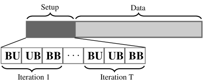
Figure 1: Frame structure.

The frame structure in Fig. 1 is split into two parts: a beamformers setup phase and data transmission phase. The over-the-air and backhaul signaling occur during the beamformers setup phase, where the over-the-air signaling is divided into two phases, more precisely, the forward precoded pilot transmission from BS to the users, denoted as BU, which occurs in lines 2 and 16 of Algorithm 2, and the backward signaling from each user to its serving BS, namely UB, which occurs in line 13 of Algorithm 2. Finally, the backhaul signaling is used to share the weights $\{\bm{\theta}_{u,n}\}_{\forall(u\in\mathcal{U}_{t},n)}$ between BS in line 14 of Algorithm 2, which is denoted as BB. The signaling exchange for a multicell MU-MIMO with two BS is illustrated in Fig. 2.

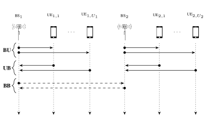
Figure 2: Signaling exchange illustration in a multicell MIMO-OFDM scenario.

VI-C Computational Complexity and Signaling Overhead

The computational complexity of the decentralized algorithm (i.e., Algorithm 2) is dominated by the matrix inversion in (10) and (20), and the MSE computation in (11). It should be noted that (10), (11) and (20) are also required by the conventional WMMSE approaches in [13, 22, 35], which correspond to the baseline algorithms considered in this paper. Therefore, the per-iteration and per-subchannel computational complexity of (10), (11) and (20) is in the order $\mathcal{O}(U^{2}N_{T}N_{R}^{2}+U^{2}N_{T}^{2}N_{R}+U^{2}N_{T}^{3}+UN_{R}^{3})$. Therefore, assuming that the computation of other variables can be solved by linear expressions, whose contribution to the overall complexity can be ignored, the per-iteration and per-subchannel computational complexity of the proposed solution is also in the order $\mathcal{O}(U^{2}N_{T}N_{R}^{2}+U^{2}N_{T}^{2}N_{R}+U^{2}N_{T}^{3}+UN_{R}^{3})$. Such a per-iteration computational complexity can be easily handled by current base stations and user devices for a moderate number of transmit/receive antennas.

In addition, the proposed solution can be implemented in a distributed fashion by applying a precoded pilot signaling scheme, which is described in Section VI-B. In that signaling scheme, each iteration has an associated overhead due to the transmission of precoded uplink/downlink pilots. Based on [50], we can measure the communication overhead by the number of orthogonal pilot symbols needed for each iteration, which is given by $\Omega=2TBU_{b}S$, where $T$ is the number of iterations. Thus, the minimum number of orthogonal pilots, $\Omega$, increases with the number of data streams, base stations, users, and iterations. Therefore, increasing the number of inner iterations of Algorithm 2 incurs a higher signaling overload. Thus, in order to obtain a practical implementation of Algorithm 2 with minimal signaling overhead, this number of iterations can be limited to a maximum of 10 iterations per data frame, as suggested in [50], at the cost of a possibly lower performance in some situations. Under these conditions, the proposed decentralized algorithm has the potential to handle moderate latency-sensitive applications.

Considering the above discussion, we conclude that the proposed solution has a computational complexity comparable with that of existing solutions, which can be handled by existing hardware, and can be efficiently deployed based on the proposed precoded pilot scheme.

VII Performance Evaluation

In this section we present the simulation setting and simulation results. More precisely, Section VII-A details the simulation setup. The convergence analysis of the proposed solutions is conducted in Section VII-B, while the performance evaluation using a Poisson traffic model is presented in Section VII-C. Section VII-D shows the performance of the proposed solution under a bursty traffic model and, finally, we analyze the impact of imperfect CSI in Section VII-E.

VII-A Simulation Assumptions

We consider the downlink of multicell MU-MIMO OFDM scenarios where each BS is located at the center of a hexagonal cell and the users are uniformly distributed within the cell. We set the inter-site distance to 250 m. Moreover, uniform linear arrays are employed by all UE and BS. The BS and UE heights are 25 m and 1.5 m, respectively, and the UE speed is equal to 3 km/h. The 5G-StoRM [39, 40], assuming the UMi scenario, is used for all links, considering a carrier frequency of 2 GHz and that each sub-channel has a bandwidth of 180 kHz. More details about the channel generation can be found in [39, 40]. For all analyzed scenarios, the power budget is $P_{b}$ = 35 dBm, $\forall b\in\mathcal{B}$ and the step size, $\rho^{(k)}$, is fixed to be equal to 0.01. Also, every user has the same average packet arrival rate and packet size in the simulation. Unless otherwise stated, $\bar{L}_{u,m}=9600$ bits. Based on [51], the maximum outage probability and the maximum tolerable latency are set as 0.05 and 20 ms, respectively (i.e., $\xi=0.05$ and $d_{\max}=20$ ms). The simulations are performed during 300 time slots or TTI, where each TTI has a duration of 1 ms. Also, the results are obtained from 100 Monte-Carlo simulations.

We consider three state-of-the-art solutions for performance comparison against our proposed solution. The first solution is the WMMSE algorithm [13], which solves a weighted sum-rate maximization problem without QoS constraints. The second solution is the JSFRA algorithm [35], which minimizes the total number of backlogged packets in each TTI. Finally, we also consider the algorithm proposed in [22], which solves the weighted sum-rate maximization problem with minimum rate requirements (hereafter, the solution from [22] is referred to as Kaleva). Note that both WMMSE and Kaleva algorithms were conceived assuming a full-buffer model, while the JSFRA solution considers a finite-buffer model.

VII-B Convergence Analysis

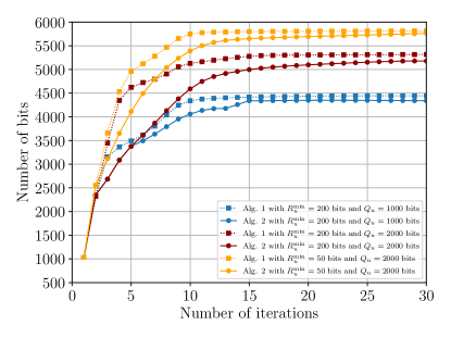
Figure 3: Convergence of the total number of transmitted bits for Algs. 1 and 2 with $\{B,U,U_{b},N,N_{\text{T}},N_{\text{R}}\}=\{2,6,3,1,8,2\}$.

Fig. 3 depicts the total number of transmitted bits as a function of the number of iterations for different values of $R_{u}^{\min}$ and $Q_{u}$. The proposed solutions converges to the final solution with a low number of iterations. Moreover, when $Q_{u}$ increases, for a fixed value of $R_{u}^{\min}$, the proposed solutions achieve a higher number of transmitted bits. In general, users with good channel conditions should diminish their data rate in order to avoid over-allocation of resources. However, when $Q_{u}$ increases, more bits are available in the buffers, thus, these users can transmit more data and, consequently, increase the system total data rate. On the other hand, when we increase the minimum number of transmitted bits required per user, $R_{u}^{\min}$, for a fixed value of $Q_{u}$, we observe that the number of transmitted bits achieved by the proposed algorithm diminishes. The reason behind this is that the proposed solution allocates more resources to users in poor channel conditions in order to fulfill the minimum number of transmitted bits for all users, consequently, diminishing the total number of transmitted bits. Finally, comparing the performance of the proposed solutions, we can see that the proposed decentralized solution (Algorithm 2) performs very close to the centralized solution (Algorithm 1) in terms of number of transmitted bits for different data rate requirements. However, we remark that the centralized solution requires an initial feasible point of problem (15) to start the iterations in Algorithm 1, which demands high computational complexity. On the other hand, the decentralized solution presents a better trade-off between performance and computational complexity. Consequently, we use only the decentralized solution for further performance evaluations.

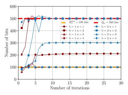
Figure 4: Convergence of the number of transmitted bits for all users with $\{B,U,U_{b},N,N_{T},N_{R},R_{u}^{\min},Q_{u}\}=\{2,8,4,1,4,2,100,500\}$.

In Fig. 4, we show the convergence of the number of transmitted bits for all users for Algorithm 2. In the first iterations of the algorithm, only part of the users are assigned with a number of transmitted bits higher than the minimum requirement. Nevertheless, as the algorithm converges, it adjusts the number of transmitted bits for the remaining users in order to fulfill the minimum requirement for all users. Moreover, it can be seen that some users, specially those with high channel gains, have the potential to transmit more bits than the number of available bits in their buffers. However, as the proposed solution converges, it reduces the amount of assigned transmitted bits for those users in order to avoid over-allocation of the resources. Finally, it is worth highlighting that only a low number of iterations is needed to achieve a good solution. In the case illustrated in Fig. 4, for example, 10 iterations would be enough to assure that all users are transmitting an amount of bits between $R_{u}^{\min}$ and $Q_{u}$.

VII-C Poisson Traffic Model

As previously mentioned, the Poisson traffic model still plays an important role in practice, as it is used for evaluation purposes in 3GPP analyses. Therefore, this subsection is concerned with a performance analysis considering a Poisson traffic model.

Fig. 5 presents the outage probability versus the average arrival rate of packets, $\lambda_{u}$. For this analysis, we consider two different setups: (I) in the first setup, the user weights are set to 1 for all users, i.e., $\beta_{u}=1,\ \forall u\in\mathcal{U}_{t}$; and (II) in the second setup, four different user weights are assigned to the users. Specifically, as we have 4 users per BS, each user of a given BS has a different weight. These user weights are kept fixed within each Monte-Carlo simulation, but change for different users in different Monte-Carlo simulations. In this work, we assume two cases for the second setup: $\beta_{u}\in\{1,\ 3,\ 5,\ 7\}$ and $\beta_{u}\in\{1,\ 0.1,\ 0.01,\ 0.001\}$

First, we can observe that the outage probability increases as the average packet arrival rate increases for all solutions. This occurs because more packets arrive at the users’ buffers, leading to an increase in the waiting time of packets, consequently, increasing the number of outages.

Also, note that different user weights have a significant impact on the WMMSE performance. In fact, this is expected because the WMMSE algorithm allocates more resources to users with high priority (higher user weights) in order to maximize the weighted sum-rate without considering the minimum data rate demands, leading to an increase in the outage probability. Regarding the JSFRA algorithm, we observe an increase in the outage probability when $\beta_{u}=\{1,0.1,0.01,0.001\}$. The reason for this is that, as the users’ weights are not relatively close, the JSFRA algorithm tends to prioritize the users with high priority instead of the users with a higher number of queued packets. Consequently, the users with a higher number of queued packets tend to accumulate more bits in their buffers, affecting the outage probability performance of this solution. On the other hand, the outage probability of the Kaleva and the proposed solution remains almost unchanged for all setups. This occurs because the average outage probability is related to minimum data rate requirements, which are not changed in both cases. Differently from the WMMSE and JSFRA algorithms, both the Kaleva and the proposed solutions take into account minimum QoS requirements. Consequently, even prioritizing the users with a higher priority, these solutions aim at meeting the QoS constraints of each user, which causes a more fair distribution of the resources among users. Moreover, importantly, the proposed solution takes into account that the sum of the bits transmitted to a given user cannot be higher than the number of bits in its buffer in order to avoid excessive allocation of the resources. Therefore, although the users with higher weights can contribute more to increase the objective function (weighted sum-rate), their contribution is limited by their respective buffers’ length.

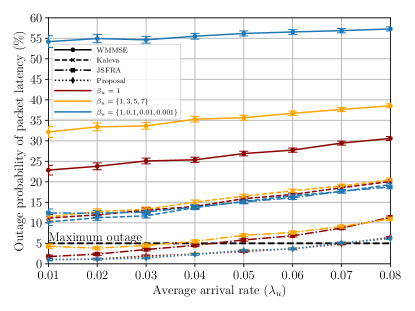
Figure 5: Performance analysis regarding the outage probability with $\{B,U,U_{b},N,N_{\text{T}},N_{\text{R}}\}=\{4,16,4,4,8,2\}$.

In addition, one can see that the WMMSE and Kaleva algorithms present the worst performance in terms of outage among the analyzed solutions. The main reason is that these solutions assume a full-buffer model. Furthermore, the WMMSE solution prioritizes the users with best channel conditions without considering minimum per-user rate requirements, thus, increasing the number of outages for packets of users in worst channel conditions. The Kaleva solution, on the other hand, takes into account minimum per-user rate requirements, which makes its performance better than the one of the WMMSE solution. Nevertheless, the outage probability obtained by the Kaleva solution is still higher than the maximum outage probability allowed. This occurs because, according to Proposition 1, it tries to fulfill the minimum requirements for all users, even though some users do not have bits to be transmitted.

We can also see that the JSFRA solution is able to maintain low outage probability values for low values of $\lambda_{u}$ and the users’ priorities are relatively the same. The reason is that the JSFRA solution aims to minimize the total number of backlogged packets in each TTI, which indirectly focuses on delay constraints. However, in general, this solution prioritizes users with a higher number of bits in their buffers before considering the users with a smaller number of bits, thus, when $\lambda_{u}$ increases, users with worst channel conditions tend to accumulate more bits and, consequently, are prioritized. However, those users are not able to achieve high data rates, which increases the waiting time of packets from those users, causing outages.

Finally, the proposed solution is able to maintain the outage probability below the maximum allowed value for almost the entire simulated range of $\lambda_{u}$. Unlike the Kaleva solution, the proposed algorithm focuses only on users with buffers that are not empty, thus, it can dedicate more resources to those users and fulfill their minimum rate requirements, which is sufficient to guarantee a low outage. Note that by guaranteeing the minimum data rate for each user, the proposed algorithm overcomes the problems related to the JSFRA solution. In fact, in the first setup, the JSFRA solution maintains the outage probability less than the maximum allowed value for $\lambda_{u}\leq 0.045$ while the proposed solution is able to fulfill the outage requirement for $\lambda_{u}\leq 0.072$, yielding a gain of 60% in terms of supported load. Moreover, for $\lambda_{u}=0.06$, the proposed solution presents a reduction of 43% of the outage rate compared to the JSFRA solution. Note that these gains compared to the state-of-art algorithms increase for the case in which $\beta_{u}=\{1,\ 0.1,\ 0.01,\ 0.001\}$.

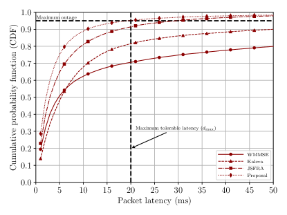
Figure 6: CDF of packet latency using a Poisson traffic model with parameters $\{B,U,U_{b},N,N_{\text{T}},N_{\text{R}},\beta_{u},\lambda_{u}\}=\{4,16,4,4,8,2,1,0.07\}$.

Up to this point, we have shown that the proposed solution is able to guarantee the outage probability for several packet arrival rates. Although this indicates that the packet latency is within the allowed range, it does not provide details about the latency of the packets. Therefore, in Fig. 6 we present the CDF of the latency of the packets for all solutions with $\lambda_{u}=0.07$ and $\beta_{u}=1$ for all users. As we can see, the curve of the proposed solution is more to the left, which means that it achieves the lowest latencies. In fact, we can observe that, approximately, 80% of the packet latencies obtained by the proposed solution are mainly distributed within 1 and 6 ms, while the percentage of packets with latency higher than the maximum tolerable latency is strictly less than the maximum outage probability allowed, which means that the proposed solution can satisfy the latency requirements. In addition, at the 50th and 90th percentiles, the proposed solution presents gains of 27% and 39% compared to the JSFRA solution, respectively.

VII-D Bursty Traffic Model

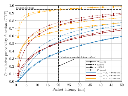
Figure 7: CDF of packet latency assuming bursty traffic scenario with parameters $\{B,U,U_{b},N,N_{T},N_{R},B_{u}\}=\{4,16,4,4,8,2,1\}$.

In some applications, the arrival of packets is bursty, which cannot be captured by the Poisson traffic model. Thus, in this section, we show how our proposed decentralized solution and the comparison algorithms perform in the presence of a bursty traffic model. For that purpose, we consider a semi-Markov ON-OFF process [52, 53] to model the bursty traffic, where the data traffic pattern is assumed to be i.i.d. among the users. Moreover, we use a Pareto random variable to model the duration of the ON state of user $u$, denoted by $\Delta_{u}^{\text{ON}}$, where $\mu_{u}$ and $\omega_{u}$ are the shape and scale parameters, respectively. The shape parameter $\mu_{u}$ determines the slope of the Pareto PDF, such that increasing values of $\mu_{u}$ decrease the variance of the variable and concentrate it near 0. Similar to [52], we set $\mu_{u}$ equal to 2. The scale parameter $\omega_{u}$, in its turn, represents the minimum value of the Pareto random variable, which means that the ON state duration would be definitely greater than $\omega_{u}$ time slots. In our simulations, we set $\omega_{u}$ to be equal to 10. Also, we model the duration of the OFF state of user $u$, denoted by $\Delta_{u}^{\text{OFF}}$, using an exponential random variable with $\delta_{u}$ representing the rate of the exponential distribution, which is set to 100 during the simulation. In addition, during the ON state, user $u$ continuously receives one packet per time slot with size equal to $Z_{u}$ bits, while during the OFF state it is idle and has no data to receive. Using this model, to compute the minimum data rate requirement using Proposition 1, we set $\lambda_{u}$ and $\bar{L}_{u,m}$ equal to 1 and $Z_{u}$, respectively.

In Fig. 7, we present a CDF of the packet latency for all algorithms assuming the bursty traffic scenario. The packet latency increases as the packet size increases for all solutions, which is an expected behavior since with higher packet sizes the traffic becomes more intense. The proposed solution presents the lowest values of packet latency compared to the other solutions considering all traffic loads. Note that the proposed solution fails to meet the outage requirements when the packet sizes are equal to 6400 and 9600 bits. The reasoning for this is that, during the ON state, the arrival rate of packets is constant, thus, the minimum data rate requirement is increased according to Proposition 1. Then, fulfilling these rate demands becomes even more difficult, which leads to a large number of backlogged packets and, consequently, higher values of outage. Even in this situation, we observe that for small packet sizes, the proposed solution is able to fulfill the outage demands, which shows that the proposed solution could be applied for low-intensity bursty traffic scenarios.

VII-E Imperfect Channel State Information

During the derivation of Algorithms 1 and 2, we assumed that perfect CSI is available at the transmitters and receivers, which can be very difficult to be obtained in practical systems. In this subsection, we analyze the performance of the proposed distributed solution (i.e., Algorithm 2) and comparison algorithms under imperfect CSI. For that, we modeled the CSI imperfection by assuming that the BS estimate the channel using an MMSE estimator. Thus, the estimated channel matrix satisfies [54, 55]: $\hat{\mathbf{H}}_{b_{i},u,n}=\varrho\mathbf{H}_{b_{i},u,n}+\sqrt{1-\varrho^{2}}\bm{\Gamma}$, where $\bm{\Gamma}\in\mathbb{C}^{N_{R}\times N_{T}}$ is an error matrix with complex Gaussian i.i.d. entries with zero mean and unit variance, while ${0\leq\varrho\leq 1}$ denotes the reliability of the channel estimation. The $\varrho$ parameter is set in such a way that the MSE between the estimated channel matrix and the actual one is approximately -10 dB and -5.7 dB, reflecting different reliability scenarios.

Fig. 8 presents the CDF of the values of packet latency for all analyzed solutions considering different levels of CSI imperfection. Again, the curve of the proposed solution is more to the left, thereby, it achieves the lowest values of packet latency. In addition, we have that the JSFRA, Kaleva and the WMMSE solutions are drastically affected by channel estimation errors. Meanwhile, we can see that the proposed solution is still able to fulfill the demands of the system when the channel estimation errors are low. Indeed, when the MSE is equal to -10 dB, the percentage of packets with latency higher than the maximum tolerable latency is strictly less than the maximum allowed outage probability. Thus, even under the effects of channel estimation errors, the proposed solution meets the data rate requirements and, consequently, the outage probability. This is an interesting result because the proposed solution does not consider the channel errors in its modeling and even so it can satisfy the outage requirements. When the channel estimation error increases, i.e., MSE = -5.7 dB, we observe that the outage probability of the proposed solution increases to, approximately, 11%, which is higher than the maximum allowed. However, the proposed solution achieves a gain of 38% compared to the JSFRA solution in this situation. Improving the performance of the proposed solution with imperfect CSI is out of the scope of this paper and is left as a perspective for future works.

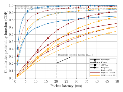
Figure 8: CDF of packet latency with different levels of CSI imperfection and parameters $\{B,U,U_{b},N,N_{T},N_{R},\beta_{u},\lambda_{u}\}=\{4,16,4,4,8,2,1,0.01\}$.

VIII Conclusions

In this work, we investigated a variant of the weighted sum-rate maximization problem subject to latency outage probability constraints in multicell MU-MIMO OFDM systems with a finite buffer model. The initially formulated problem was verified to be non-convex and very difficult to be optimally solved. It was then reformulated and solved, iteratively, up to a locally optimal point by using the max-plus queuing method from network analysis, the well known MSE-SINR relation when using MMSE, as well as SCA. In addition, a decentralized solution with relaxed feasible initialization requirements was proposed based on the dual decomposition and Lagrangian relaxation of the rate constraints. Also, signaling aspects for practical implementation of the decentralized solution and a detailed convergence analysis were provided.

Unlike previous works, a more realistic channel model was utilized with space, frequency and time correlations. The numerical results showed that the proposed framework outperforms state-of-the-art algorithms in terms of outage probability and latency for different scenarios. Indeed, compared to the benchmarking solutions, the proposed solution presented a reduction of approximately 43% of outage probability and a gain of 60% in terms of the supported load in scenarios where users have equal user weights. Thus, we conclude that the proposed solutions present the currently available best performance to the stated problem considering the existing methods to solve such problems. Finally, as perspective for further studies, we indicate the development of solutions that take into account channel estimation and extensions of the proposed framework using other traffic models.

Appendix A
Convergence Analysis

In this appendix, we perform the converge analysis for both centralized and decentralized algorithms, which is based on [22]. We assume a sufficient number of inner subgradient iterations for both centralized and decentralized algorithms. In other words, in order to guarantee monotonic improvement with respect to the objective function after each transmit beamformers iteration, Algorithms 1 and 2 perform enough subgradient updates [56, 48].

Remark 1

Several iterations of the dual decomposition and SCA updates can be performed in the inner loops of Algorithms 1 and 2 during the updates of the variables $\{\hat{r}_{u,n}\}_{\forall(u\in\mathcal{U}_{t},n)}$ and the transmit beamformers $\{\mathbf{M}_{u,n}\}_{\forall(u\in\mathcal{U}_{t},n)}$. The number of inner updates should guarantee the monotonicity regarding the global objective function.

We follow our analysis by showing that the feasible set of (13) is compact. Since the power constraints in (6b) are convex and compact, we have that the feasible set of the transmit beamformers $\{\mathbf{M}_{u,n}\}_{\forall(u\in\mathcal{U}_{t},n)}$ is convex and compact. Analogously, the feasible set of the variables $\{\hat{r}_{u,n}\}_{\forall(u\in\mathcal{U}_{t},n)}$ is also convex and compact. Moreover, since the noise power is non-zero, the receive covariance matrix in (10) is always invertible and, consequently, the mapping between the transmit and receive beamformer is a continuous map [56]. Based on that the set comprising the feasible MMSE receive beamformers $\{\mathbf{W}_{u,n}\}_{\forall(u\in\mathcal{U}_{t},n)}$ is closed and bounded, which shows that such a set is also compact. Finally, we can represent the updates iterations of the variables $\{\hat{r}_{u,s,n}\}_{\forall(u\in\mathcal{U}_{t},s,n)}$, as well as the receive and transmit beamformers, using infimal maps [22, 57]. According to [57], since the set of all optimization variables is compact, as stated before, the infimal maps modeling the updates of the optimization variables are closed point-to-set maps.

Proposition 2

The objective function of problem (13) is monotonic and converges with Algorithm 1.

Proof:

The MMSE receivers are the unique rate optimal receivers for problem (13) in the sense that they maximize the per-stream SINR, i.e., they maximize the rate for each user [22, 19]. Then, we can conclude that the objective of problem (13) is strictly increasing for each receive beamformer update given by (10). Also, it was shown in [47] that the solution of the SCA subproblem in Algorithm 1 is either a solution of the original problem or the objective is monotonically improved. Furthermore, given Remark 1, the monotonicity is extended to Algorithm 2. Finally, since the objective is bounded by the power and rate constraints, we can claim the convergence of the objective function in problem (13) when executing Algorithm 1 and Algorithm 2. ∎

Once we have shown that the algorithms can be modeled as closed infimal maps and are monotonic with respect to the objective function of problem (13), it follows from the convergence theorem in [58] that the sequence of iterates generated by Algorithm 1 and Algorithm 2 has at least one accumulation point and each accumulation point is a generalized fixed point.

However, we can make the convergence results stronger and show that the Algorithms 1 and 2 converge to a unique solution for all fixed points. Indeed, we can obtain this behavior by using a uniquely defined generalized inverse operation, such as the Moore-Penrose pseudoinverse, in (20) [22]. Nevertheless, we have that the set of the feasible fixed points is infinite, since there is an SINR equivalence for different complex beamformers with some different phase rotation, consequently, convergence to a single fixed point cannot be guaranteed [59].

Then, we should show that any fixed point of Algorithm 1 is a KKT point of problem (9).

Proposition 3

Any fixed limit point $\{\mathbf{W}_{u,n}^{\ast},\mathbf{M}_{u,n}^{\ast},\hat{r}^{\ast}_{u,n},\mathbf{E}_{u,n}^{\ast}\}_{\forall(u\in\mathcal{U}_{t},n)}$ of Algorithm 1 is a KKT point of problem (9).

Proof:

Based on [47], where it was shown that the SCA algorithm stops at a KKT point, or the limit of any convergent sequence is a KKT point, with a slight difference due to the extra step involving the receive beamformer updates. That said, we have that the primal and dual constraints always hold for problem (9), since the convex approximation is only applied for the constraints (14). Consequently, we can focus only on the constraints affected by SCA.

Let us start by defining $\varUpsilon(\mathbf{E}_{u,n},\mathbf{E}_{u,n}^{(k)})$ as the first-order Taylor approximation around a fixed MSE point in (14). Thus, from the convergence to a fixed point and definition of the first-order linear approximation, we have that $-\log_{2}\det\left(\mathbf{E}_{u,n}^{\ast}\right)=\varUpsilon(\mathbf{E}_{u,n}^{\ast},\mathbf{E}_{u,n}^{\ast})$ and $\frac{-\partial\log_{2}\det\left(\mathbf{E}_{u,n}^{\ast}\right)}{\partial\mathbf{E}_{u,n}}=\frac{\partial\ \varUpsilon(\mathbf{E}_{u,n}^{\ast},\mathbf{E}_{u,n}^{\ast})}{\partial\mathbf{E}_{u,n}},\ \forall(u\in\mathcal{U}_{t},n)$. Thus, by definition, we have that the first-order optimality conditions hold. In addition, the MSE as well as transmit and receive beamformers in (11), (20) and (10), respectively, are directly solved from the first-order optimality conditions, which means that they also satisfy the optimality conditions. Regarding the complementary slackness conditions, it is easy to see that the constraints (14) hold tight at any fixed point, consequently, $\hat{r}_{u,n}=\varUpsilon(\mathbf{E}_{u,n}^{\ast},\mathbf{E}_{u,n}^{\ast})\Rightarrow\psi_{u,n}^{\ast}(\hat{r}_{u,n}^{\ast}-\varUpsilon(\mathbf{E}_{u,n}^{\ast},\mathbf{E}_{u,n}^{\ast}))=0,\ \forall(u\in\mathcal{U}_{t},n)$. Similar analyses also apply for the rate and MSE constraints. In addition, we can also observe that, since the linear approximation generates a lower bound for convex functions, the primal feasibility holds, i.e., $\hat{r}_{u,n}^{\ast}\leq\varUpsilon(\mathbf{E}_{u,n}^{\ast},\mathbf{E}_{u,n}^{\ast})\leq-\log_{2}\det\left(\mathbf{E}_{u,n}^{\ast}\right)$. Then, we can conclude that any fixed point is also a KKT point of problem (9), which was also observed in [47]. The equivalence between a KKT point of (9) and (13) follows directly from the well-known relation between MSE and SINR when using MMSE receivers [12, 13], for which a similar rigorous proof is shown in [13]. ∎

References

- [1] Ericsson, “Ericsson mobility report: Q4 2019 update,” Feb. 2020. [Online]. Available: https://www.ericsson.com/491b06/assets/local/mobility-report/documents/2019/ericsson-mobility-report-q4-2019-update.pdf
- [2] J. Navarro-Ortiz, P. Romero-Diaz, S. Sendra et al., “A survey on 5G usage scenarios and traffic models,” IEEE Commun. Surveys Tuts., Feb. 2020, to be published.
- [3] G. J. Sutton, J. Zeng, R. P. Liu et al., “Enabling technologies for ultra-reliable and low latency communications: From PHY and MAC layer perspectives,” IEEE Commun. Surveys Tuts., vol. 21, no. 3, pp. 2488–2524, Feb. 2019.
- [4] M. Agiwal, A. Roy, and N. Saxena, “Next generation 5G wireless networks: A comprehensive survey,” IEEE Commun. Surveys Tuts., vol. 18, no. 3, pp. 1617–1655, Feb. 2016.
- [5] A. A. Zaidi, R. Baldemair, H. Tullberg et al., “Waveform and numerology to support 5G services and requirements,” IEEE Commun. Mag., vol. 54, no. 11, pp. 90–98, Nov. 2016.
- [6] L. Yu, E. Karipidis, and E. G. Larsson, “Coordinated scheduling and beamforming for multicell spectrum sharing networks using branch and bound,” in Proc. of the European Signal Processing Conference (EUSIPCO), Aug. 2012, pp. 819–823.
- [7] P. Ameigeiras, Y. Wang et al., “Traffic models impact on OFDMA scheduling design,” EURASIP Journal on Wireless Communications and Networking, vol. 2012, no. 61, pp. 1–13, Feb. 2012.
- [8] N. Wei, A. Pokhariyal et al., “Performance of spatial division multiplexing MIMO with frequency domain packet scheduling: From theory to practice,” IEEE J. Sel. Areas Commun., vol. 26, no. 6, pp. 890–900, Aug. 2008.
- [9] Y. Gao, L. Chen, X. Zhang, and Y. Jiang, “Performance evaluation of mobile wimax with dynamic overhead,” in Proc. of the IEEE Vehicular Technology Conference, Oct. 2008, pp. 1–5.
- [10] E. Castañeda, A. Silva, A. Gameiro, and M. Kountouris, “An overview on resource allocation techniques for multi-user MIMO systems,” IEEE Commun. Surveys Tuts., vol. 19, no. 1, pp. 239–284, Firstquarter 2017.
- [11] O. Oguejiofor and L. Zhang, “Global optimization of weighted sum-rate for downlink heterogeneous cellular networks,” in Proc. of the Internat. Conf. on Telecommun. (ICT), Jun. 2016, pp. 1–6.
- [12] S. S. Christensen, R. Agarwal, E. D. Carvalho, and J. M. Cioffi, “Weighted sum-rate maximization using weighted MMSE for MIMO-BC beamforming design,” IEEE Trans. Wireless Commun., vol. 7, no. 12, pp. 4792–4799, Dec. 2008.
- [13] Q. Shi, M. Razaviyayn, Z. Luo, and C. He, “An iteratively weighted MMSE approach to distributed sum-utility maximization for a MIMO interfering broadcast channel,” IEEE Trans. Signal Process., vol. 59, no. 9, pp. 4331–4340, Sep. 2011.
- [14] K. Shen and W. Yu, “Fractional programming for communication systems - part I: Power control and beamforming,” IEEE Trans. Signal Process., vol. 66, no. 10, pp. 2616–2630, May 2018.
- [15] M. Codreanu, A. Tölli, M. Juntti, and M. Latva-aho, “Joint design of Tx-Rx beamformers in MIMO downlink channel,” IEEE Trans. Signal Process., vol. 55, no. 9, pp. 4639–4655, Sep. 2007.
- [16] K. Shen, W. Yu, L. Zhao, and D. P. Palomar, “Optimization of MIMO device-to-device networks via matrix fractional programming: A minorization-maximization approach,” IEEE/ACM Trans. Netw., vol. 27, no. 5, pp. 2164–2177, 2019.
- [17] Q. Shi, M. Razaviyayn, M. Hong, and Z. Luo, “SINR constrained beamforming for a MIMO multi-user downlink system: Algorithms and convergence analysis,” IEEE Trans. Signal Process., vol. 64, no. 11, pp. 2920–2933, Jun. 2016.
- [18] A. Tölli, H. Pennanen, and P. Komulainen, “Decentralized minimum power multi-cell beamforming with limited backhaul signaling,” IEEE Trans. Wireless Commun., vol. 10, no. 2, pp. 570–580, Feb. 2011.
- [19] H. Pennanen, A. Tölli et al., “Decentralized linear transceiver design and signaling strategies for sum power minimization in multi-cell MIMO systems,” IEEE Trans. Signal Process., vol. 64, no. 7, pp. 1729–1743, apr 2016.
- [20] F. Han, S. Zhao et al., “Decentralized beamforming for weighted sum energy efficiency maximization in MIMO systems,” in Proc. of the IEEE Global Commun. Conf. (GLOBECOM), Dec. 2017, pp. 1–6.
- [21] Y. Yang, M. Pesavento et al., “Energy efficiency optimization in MIMO interference channels: A successive pseudoconvex approximation approach,” IEEE Trans. Signal Process., vol. 67, no. 15, pp. 4107–4121, June 2019.
- [22] J. Kaleva, A. Tölli, and M. Juntti, “Decentralized sum rate maximization with QoS constraints for interfering broadcast channel via successive convex approximation,” IEEE Trans. Signal Process., vol. 64, no. 11, pp. 2788–2802, Jun. 2016.
- [23] R. P. Antonioli, G. Fodor, P. Soldati, and T. F. Maciel, “User scheduling for sum-rate maximization under minimum rate constraints for the MIMO IBC,” IEEE Wireless Commun. Lett., vol. 8, no. 6, pp. 1591–1595, Dec. 2019.
- [24] R. P. Antonioli, G. Fodor, P. Soldati, and T. F. Maciel, “Decentralized user scheduling for rate-constrained sum-utility maximization in the MIMO IBC,” IEEE Trans. Commun., pp. 1–1, Jul. 2020.
- [25] N. U. Hassan and M. Assaad, “Low complexity margin adaptive resource allocation in downlink MIMO-OFDMA system,” IEEE Trans. Wireless Commun., vol. 8, no. 7, pp. 3365–3371, July 2009.
- [26] P. Tejera, W. Utschick, J. A. Nossek, and G. Bauch, “Rate balancing in multiuser MIMO OFDM systems,” IEEE Trans. Commun., vol. 57, no. 5, pp. 1370–1380, May 2009.
- [27] F. R. M. Lima, T. F. Maciel et al., “Improved spectral efficiency with acceptable service provision in multiuser MIMO scenarios,” IEEE Trans. Veh. Technol., vol. 63, no. 6, pp. 2697–2711, Nov. 2014.
- [28] F. R. M. Lima, N. S. Bezerra et al., “Maximizing spectral efficiency with acceptable service provision in multiple antennas scenarios,” in Proc. of the European Wireless Conference, Apr. 2012, pp. 1–8.
- [29] W. Yu, T. Kwon, and C. Shin, “Multicell coordination via joint scheduling, beamforming, and power spectrum adaptation,” IEEE Trans. Wireless Commun., vol. 12, no. 7, pp. 1–14, June 2013.
- [30] Kibeom Seong, R. Narasimhan, and J. M. Cioffi, “Queue proportional scheduling via geometric programming in fading broadcast channels,” IEEE J. Sel. Areas Commun., vol. 24, no. 8, pp. 1593–1602, July 2006.
- [31] J. Mei, K. Zheng et al., “A latency and reliability guaranteed resource allocation scheme for LTE V2V communication systems,” IEEE Trans. Wireless Commun., vol. 17, no. 6, pp. 3850–3860, Jun. 2018.
- [32] G. Venkatraman, A. Tölli et al., “Low complexity multiuser MIMO scheduling for weighted sum rate maximization,” in Proc. of the European Signal Process. Conf. (EUSIPCO), Sep. 2014, pp. 820–824.
- [33] S. Lakshminarayana, M. Assaad, and M. Debbah, “Energy efficient design in MIMO multi-cell systems with time average QoS constraints,” in Proc. of the IEEE Workshop on Signal Processing Advances in Wireless Communications (SPAWC), Sep. 2013, pp. 614–618.
- [34] B. Niu, V. W. S. Wong, and R. Schober, “Downlink scheduling with transmission strategy selection for multi-cell MIMO systems,” IEEE Trans. Wireless Commun., vol. 12, no. 2, pp. 736–747, Dec. 2013.
- [35] G. Venkatraman, A. Tölli, M. Juntti, and L. Tran, “Traffic aware resource allocation schemes for multi-cell MIMO-OFDM systems,” IEEE Trans. Signal Process., vol. 64, no. 11, pp. 2730–2745, Jun. 2016.
- [36] G. Venkatraman, A. Tölli, M. Juntti, and L. Tran, “Queue aware precoder design via OTA training,” in Proc. of the IEEE 17th International Workshop on Signal Processing Advances in Wireless Communications (SPAWC), Aug. 2016, pp. 1–6.
- [37] Q. Du and X. Zhang, “QoS-aware base-station selections for distributed MIMO links in broadband wireless networks,” IEEE J. Sel. Areas Commun., vol. 29, no. 6, pp. 1123–1138, May 2011.
- [38] J. Li, N. Bao et al., “Adaptive user scheduling and resource management for multiuser MIMO downlink systems with heterogeneous delay requirements,” in Proc. of the IEEE Wireless Communications and Networking Conference (WCNC), Apr. 2013, pp. 1351–1356.
- [39] A. M. Pessoa, I. M. Guerreiro et al., “A stochastic channel model with dual mobility for 5G massive networks,” IEEE Access, vol. 7, pp. 149 971–149 987, Oct. 2019.
- [40] 3GPP, “TR 38.900 v14.2.0: Study on channel model for frequency spectrum above 6 GHz,” Technical Specification Group Radio Access Network, Report Release 14, 2016.
- [41] 3GPP, “TR 36.814 v9.2.0: Further advancements for e-utra physical layer aspects,” Technical Specification Group Radio Access Network, Report Release 9, 2017.
- [42] 3GPP, “TS 37.985 v16.0.0: Overall description of radio access network (RAN) aspects for vehicle-to-everything (V2X) based on LTE and NR,” ETSI, Technical Specification Release 16, Jun. 2020.
- [43] 3GPP, “TR 36.885 v14.0.0: Study on LTE-based V2X services,” ETSI Technical Specification, Technical Report Release 14, Jun. 2016.
- [44] Z.-Q. Luo and S. Zhang, “Dynamic spectrum management: Complexity and duality,” IEEE J. Sel. Areas Commun., vol. 2, no. 1, pp. 57–73, Feb. 2008.
- [45] Y. Jiang, “Network calculus and queueing theory: two sides of one coin: invited paper,” in Proc. of the Int. ICST Conf. Perform. Eval. Methodologies and Tools, 5 2010, pp. 37–48.
- [46] S. Boyd, L. Xiao et al., “Sequencial convex programming - Notes for ee364b, Stanford University,” Jan. 2007.
- [47] B. R. Marks and G. P. Wright, “Technical note — a general inner approximation algorithm for nonconvex mathematical programs,” Oper. Res., vol. 26, no. 4, pp. 681–683, Aug. 1978.
- [48] D. P. Bertsekas, Nonlinear programming, 2nd ed. Belmont, MA, USA: Athena scientific, 1999.
- [49] D. P. Palomar and Mung Chiang, “A tutorial on decomposition methods for network utility maximization,” IEEE J. Sel. Areas Commun., vol. 24, no. 8, pp. 1439–1451, Aug. 2006.
- [50] A. Tölli, H. Ghauch et al., “Distributed coordinated transmission with forward-backward training for 5G radio access,” IEEE Commun. Mag., vol. 57, no. 1, pp. 58–64, Jan. 2019.
- [51] 3GPP, “TS 22.186 v15.4.0: Service requirements for enhanced V2X scenarios,” ETSI Technical Specification, Report Release 15, 2018.
- [52] S. H. Rastegar, A. Abbasfar et al., “Rule caching in sdn-enabled base stations supporting massive IoT devices with bursty traffic,” IEEE Internet Things J., vol. 7, no. 9, pp. 8917–8931, Sept. 2020.
- [53] F. Liu, J. Riihijärvi, and M. Petrova, “Analysis of proportional fair scheduling under bursty on-off traffic,” IEEE Commun. Lett., vol. 21, no. 5, pp. 1175–1178, May 2017.
- [54] F. Rusek, D. Persson et al., “Scaling up MIMO: Opportunities and challenges with very large arrays,” IEEE Signal Process. Mag., vol. 30, no. 1, pp. 40–60, Jan 2013.
- [55] I. M. Braga Jr., E. O. Cavalcante et al., “User scheduling based on multi-agent deep Q-learning for robust beamforming in multicell MISO systems,” IEEE Commun. Lett., pp. 1–1, Aug. 2020.
- [56] S. Boyd and L. Vandenberghe, Convex optimization. Cambridge, U.K.: Cambridge University Press, 2004.
- [57] G. B. Dantzig, J. H. Folkman, and N. Shapiro, “On the continuity of the minimum set of a continuous function,” J. Math. Anal. Appl., vol. 17, no. 3, pp. 519–548, Mar. 1967.
- [58] W. I. Zangwill, “Convergence conditions for nonlinear programming algorithms,” Management Science, vol. 16, no. 1, pp. 1–13, Sep. 1969.
- [59] R. R. Meyer, “Sufficient conditions for the convergence of monotonic mathematical programming algorithms,” Journal of Computer and System Sciences, vol. 12, no. 1, pp. 108–121, Feb. 1976.