Realistic tight-binding model for monolayer transition metal dichalcogenides in 1T’ structure

Abstract

Monolayer transition metal dichalcogenides $MX_{2}$ ($M$ = Mo,W and $X$ = Te, Se, S) in 1T’ structure were predicted to be quantum spin Hall insulators based on first-principles calculations, which were quickly confirmed by multiple experimental groups. For a better understanding of their properties, in particular their responses to external fields, we construct a realistic four-band tight-binding (TB) model by combining the symmetry analysis and first-principles calculations. Our TB model respects all the symmetries and can accurately reproduce the band structure in a large energy window from -0.3 eV to 0.8 eV. With the inclusion of spin-orbital coupling (SOC), our TB model can characterize the nontrivial topology and the corresponding edge states. Our TB model can also capture the anisotropic strain effects on the band structure and the strain-induced metal-insulator transition. Moreover, we found that although $MX_{2}$ share the same crystal structures and have the same crystal symmetries, while the orbital composition of states around the Fermi level are qualitatively different and their lower-energy properties cannot fully described by a single $\bm{k\cdot p}$ model. Thus, we construct two different types of $\bm{k\cdot p}$ model for $M$S₂,$M$Se₂ and $M$Te₂, respectively. Benefiting from the high accuracy and simplicity, our TB and $\bm{k\cdot p}$ models can serve as a solid and concrete starting point for future studies of transport, superconductivity, strong correlation effects and twistronics in 1T’-transition metal dichalcogenides.

I INTRODUCTION

Since proposed in 2005,quantum spin Hall insulators (QSHIs)Kane and Mele (2005) have attracted tremendous attention due to its unexpected nontrivial topology and potential applications in next-generation information technologies. There are many theoretical predictions of QSHIs in various material systemsHasan and Kane (2010); Qi and Zhang (2011); Bansil et al. (2016). To date, however, only three material systems have exhibited quantized edge conductance in transport experiments: HgTe quantum wellsBernevig et al. (2006); König et al. (2007), InAs/GaSb quantum wellsLiu et al. (2008); Knez et al. (2011) and monolayer WTe₂-type transition metal dichalcogenides (TMDCs)Qian et al. (2014); Fei et al. (2017); Wu et al. (2018). Among them, WTe₂-type TMDCs are the most promising for potential applications of QSHIs, as they are 2D van der Waals materials.

WTe₂-type TMDCs were first predicted to be QSHIs in 2014 Qian et al. (2014) and was experimentally confirmed in WTe₂ in 2017 by several independent experiments including transportFei et al. (2017); Wu et al. (2018), angle-resolved photoemission spectroscopy (ARPES)Tang et al. (2017a) and scanning tunneling microscopy (STM)Tang et al. (2017a); Peng et al. (2017); Jia et al. (2017). Remarkably, the quantized conductance persists at a high temperature of around 100 KWu et al. (2018). Besides the nontrivial topology, the thin films of WTe₂ also possess many other interesting properties including gate-induced superconductivityPalomaki et al. (2018); Fatemi et al. (2018); Hsu et al. (2020); Xie et al. (2020) and ferroelectricityFei et al. (2018); Sharma et al. (2019). Although inversion symmetry is preserved in monolayer 1T’-WTe₂, it is broken in the bulk and multilayer thin films, which leads to the existence of Weyl pointsSoluyanov et al. (2015), Berry curvature dipoleXu et al. (2018a), and spin-orbit torquesMacNeill et al. (2017). Besides, WTe₂ also exhibits a temperature-induced Lifshitz transitionWu et al. (2015) and pressure-driven superconductivityPan et al. (2015); Kang et al. (2015).

In addition to the extensive studies of WTe₂, the exploration has also been extended to other related materials. For example, monolayer 1T’-WSe₂Chen et al. (2018); Pedramrazi et al. (2019); Chen et al. (2021) , 1T’-MoSe₂Cheng et al. (2019), 1T’-MoTe₂Naylor et al. (2016) and 1T’-MoS₂Xu et al. (2018b) are successfully fabricated; plus WSe₂ and MoS₂ show a gapped bulk and conducting edge states in experiments. Observations of topological Fermi arcsDeng et al. (2016) and superconductivityQi et al. (2016) in bulk MoTe₂ are also reported.

So far, all the experiments about monolayer WTe₂ are consistent with each other on the nontrivial topology, and transport experiments clearly show that the bulk states of monolayer WTe₂ are insulatingFei et al. (2017); Wu et al. (2018). However, on the origin of such an insulating behavior, ARPES and STM experiments give contrasting results. ARPES experiments show a non-zero single-particle gap of monolayer WTe₂ Tang et al. (2017b), while the STM experiments show that monolayer WTe₂ is gapless in the single-particle level, and the gap is from electron-electron correlation pinned at the Fermi levelSong et al. (2018). Meanwhile, there are some other strange transport behaviors varying with the gating voltage and temperature, which cannot be explained by a single-particle gapFei et al. (2017); Wu et al. (2018). A general theoretical picture of all these experimental results is crucial for future studies and applications. Although first-principles calculations can characterize the band structure of 1T’-$MX_{2}$ Qian et al. (2014), the huge computational cost makes it incapable to study correlation effects and related properties under various doping/gating, strains and electric fields.

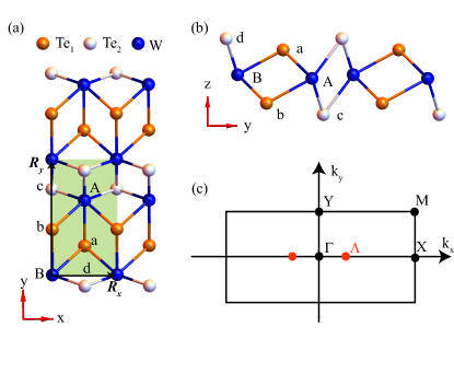
Figure 1: Crystal structure of monolayer 1T’-WTe₂. (a) top view and (b) side view of 1T’-WTe₂. For Te atoms, we divide them into two groups (labeled by Te₁ (orange) and Te₂ (white)), where two atoms in each group are connected by inversion symmetry. (c) Brillouin zone of monolayer 1T’-WTe₂. Other 1T’-$MX_{2}$ materials own the same lattice structures with different lattice constants.

Here, we build a realistic tight-binding model that can capture the low-energy physics of 1T’-$MX_{2}$ well at the level of first-principles calculations. Different from the previous worksMuechler et al. (2016); Ok et al. (2019) that can only describe the dispersion along some high symmetry lines, our model can accurately characterize the band structure in the whole Brillouin zone in a large energy window around the Fermi level from -0.3 eV to 0.8 eV for all the monolayer $MX_{2}$ in 1T’ structure. The SOC effects which open the band gaps of Dirac cones are precisely captured in our method. The SOC drives the system into a QSHI as it is in the Kane-Mele model Kane and Mele (2005). Moreover, our TB model can describe the anisotropic effects of strain on the band structure, and can correctly show the strain-induced metal-insulator phase transition. Based on the different orbital components around $\Gamma$ point, we build two types of $\bm{k\cdot p}$ model with fewer parameters. Our results here provide a solid basis for future theoretical studies of transport properties and twistronics in 1T’-$MX_{2}$. This paper is organized as follows. In Sec. II, we built two different four-band TB models with different numbers of parameters, and then showed the nontrivial topology and the edge states. In Sec. III, we introduced two types of $\bm{k\cdot p}$ model at $\Gamma$ point. In Sec. IV, the strain effects are included in the TB model. Summary is given in Sec. V.

II THE FOUR-BAND TB MODEL

	$\ \ \ \mu_{p}$	$\ \ \ \mu_{d}$	$\ \ \ d_{1}$	$\ \ \ d_{2}$	$\ \ \ d_{3}$	$\ \ \ d_{4}$	$\ \ \ d_{5}$
	$\ \ \ p_{1}$	$\ \ \ p_{2}$	$\ \ \ p_{3}$	$\ \ \ p_{4}$	$\ \ \ p_{6}$	$\ \ \ t_{1}$	$\ \ \ t_{2}$
WTe2	-1.66528	0.22665	0.44406	-0.18865	0.05731	-0.13324	–
	1.03803	0.34827	0.17243	-0.00154	–	0.99303	-0.03319
MoTe2	-1.63377	0.01866	0.28077	-0.21897	0.11990	-0.02540	–
	1.17008	0.42850	0.03297	-0.14288	–	0.88162	-0.02258
WSe2	-1.35362	0.61482	0.27092	-0.33119	0.02467	-0.03680	0.02103
	0.67497	0.15501	0.62199	-0.07087	-0.27381	0.50758	-0.11648
MoSe2	-1.29397	0.51532	0.45815	-0.20800	0.09843	-0.05272	0.09275
	0.63585	0.15681	0.10656	-0.04924	-0.00158	0.80408	-0.06020
WS2	-1.35183	0.63848	0.23062	-0.32906	0.03482	-0.04138	0.01661
	0.64428	0.12264	0.65028	-0.07014	-0.28547	0.49754	-0.04101
MoS2	-1.36700	0.62198	0.20933	-0.32600	0.03672	-0.02389	0.02699
	0.63741	0.17775	0.63298	-0.08625	-0.27196	0.53014	-0.08643

Table 1: Fitted $I$-TB model parameters for all six $MX_{2}$ in units of eV.

	$\mu_{p}$	$\mu_{d}$	$d_{1}$	$d_{2}$	$d_{3}$	$d_{4}$	$d_{5}$	$d_{6}$	$p_{1}$	$p_{2}$
	$p_{3}$	$p_{4}$	$p_{5}$	$p_{6}$	$t_{1}$	$t_{2}$	$t_{3}$	$t_{4}$	$t_{5}$	$t_{6}$
WTe2	-1.89759	0.26199	0.40510	-0.22072	-0.07897	0.17756	0.02538	–	1.13760	0.31121
	0.76753	-0.02325	–	-0.31933	0.95946	-0.25719	0.37810	-0.15573	–	–
MoTe2	-2.03758	0.03843	0.31260	-0.23191	-0.09447	0.17815	0.02140	–	1.23257	0.31056
	0.69232	-0.08343	–	-0.29010	0.81744	-0.23141	0.39989	-0.09774	–	–
WSe2	-1.3263	0.68423	0.24922	-0.26472	0.06792	-0.00247	0.02786	-0.00782	0.68267	0.22103
	0.66442	0.00497	-0.05935	-0.26452	0.75205	-0.08788	0.02258	-0.14976	-0.07251	-0.02152
MoSe2	-1.94659	0.27827	0.33844	-0.28305	-0.1167	0.20624	0.02506	0.02712	1.03571	0.25439
	0.78674	-0.0228	-0.02966	-0.33199	0.89168	-0.29952	0.37373	-0.11279	0.00868	-0.00936
WS2	-1.34342	0.87386	0.27347	-0.35576	0.05040	-0.04117	0.05692	-0.01395	0.63408	0.11487
	0.66955	0.01900	-0.09228	-0.29918	0.64972	0.00212	0.09219	-0.03392	-0.07035	0.03078
MoS2	-1.33942	0.65475	0.22663	-0.30787	0.05831	0.04386	0.00695	-0.00742	0.64578	0.17477
	0.66761	-0.01281	-0.05326	-0.28997	0.70452	-0.05753	–	-0.05290	-0.06017	0.09061

Table 2: Fitted $II$-TB model parameters for all six $MX_{2}$ in units of eV.

We first analyze the crystal symmetries of monolayer $MX_{2}$ in 1T’ structure and then build a four-band TB model based on orbital contributions from first-principles calculations. The parameters in the TB models are further fitted according to the band structure in certain energy ranges around the Fermi level.

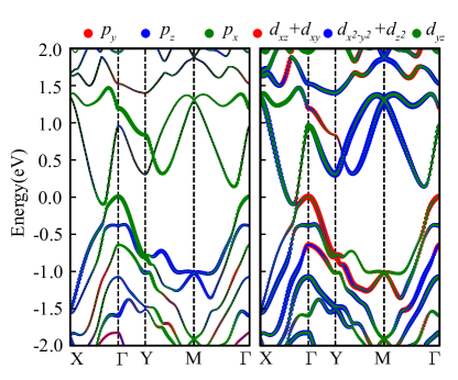
Figure 2: Orbital projections for monolayer 1T’-WTe₂ from first-principles calculations. Marker size represents the weight of a specific orbital. Left panel is projection results from $p$ orbitals of Te₁. Red for $p_{y}$, blue for $p_{z}$ and green for $p_{x}$. Right panel is the result of contributions from $d$ orbitals of W atoms, red for $d_{xz}+d_{xy}$, blue for $d_{x^{2}-y^{2}}+d_{z^{2}}$ and green for $d_{yz}$.

As shown in Fig. 1(a), monolayer 1T’-$MX_{2}$ has a rectangular unit cell with two $M$ atoms and four $X$ atoms. The lattice vectors are labeled by $\bm{R_{x}}$ and $\bm{R_{y}}$ with $z$ along the perpendicular direction, and all the unit cells can be uniquely labeled by the vector $\bm{R}_{mn}$ = $m\bm{R_{x}}$ + $n\bm{R_{y}}$, with $m,n$ $\in$ $\mathbb{Z}$.The monolayer 1T’-$MX_{2}$ belongs to a nonsymmorphic space group, containing the following symmetries: 1. Translation $\bm{T_{R}}$; 2. Glide mirror $\bar{M}_{x}$: $(x,y,z)\rightarrow(-x,y,z)+\bm{R_{x}}/2$; 3. Screw rotation $\bar{C}_{2x}$: $(x,y,z)\rightarrow(x,-y,-z)+\bm{R_{x}}/2$. There is also an inversion symmetry $P$: $(x,y,z)\rightarrow(-x,-y,-z)$, which can be written as the product of glide mirror and screw rotation $P=\bar{M}_{x}\bar{C}_{2x}$. For clarity, four $X$ atoms are divided into two types, labelled as $X_{1}$ (atoms a and b) and $X_{2}$ (atoms c and d), where two atoms in each type are connected by inversion symmetry.

The nontrivial topology of monolayer 1T’-$MX_{2}$ comes from the Peierls distortion and the strong SOCQian et al. (2014). The Peierls distortion along the $x$ axis induces a large band inversion at $\Gamma$ point, forming two gapless Dirac cones which are protected by the crystal symmetries (the $\Lambda$ points in Fig. 1(c)) along $\Gamma-X$. Moreover, the SOC can open band gaps at the Dirac points and drives monolayer 1T’-$MX_{2}$ into a Z₂ topological insulator, which is exactly the same as the Kane-Mele model for grapheneKane and Mele (2005). Here, we first build the TB model without SOC.

II.1 TB model without SOC

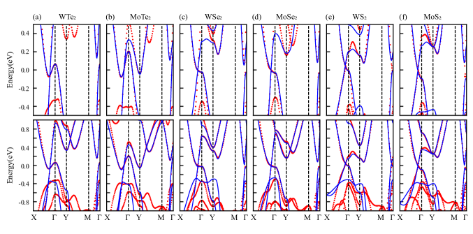
Figure 3: The $I$ - and $II$-TB fitted band structures of $MX_{2}$ with the corresponding first-principles calculations. Red dots are the first-principles calculation results and black solid lines are the fitted TB results. (a-f) Upper panel are the $I$-TB results with energy region from -0.5 eV to 0.5 eV; (a-f) Lower panel are the $II$-TB results with energy region from -1.0 eV to 1.0 eV.

The band structures of monolayer 1T’-$MX_{2}$ can be accurately calculated by first-principles calculationsQian et al. (2014); Choe et al. (2016); Tang et al. (2017a). Our first-principles calculations are performed in the framework of density functional theory as implemented in the VASP packageKresse and Furthmüller (1996) with projector augmented wave (PAW) methodBlöchl (1994). The exchange-correlation functional is Berdew-Burke-Ernzerhof (PBE)Perdew et al. (1996). The Brillouin zone is sampled in a $7\times 14\times 1$ Monkhorst-Pack k-point grid and a large vacuum region of more than 15 Å is used in the $z$ direction to minimize image interactions from the periodic boundary condition. The energy cutoff of the plane wave basis is 400 eV. The relaxed lattice constants are consistent with the previous worksQian et al. (2014); Choe et al. (2016); Tang et al. (2017a).

To be more specific, we focus on WTe₂ in the following part. As shown in Fig. 2, the states in the energy window from -0.5 eV to 1.0 eV are mostly contributed by $\{d_{x^{2}-y^{2}},d_{z^{2}}\}$ orbitals of W atom and $p_{x}$ orbital of Te₁ atom, which belong to the irreducible representations (IRs) $A_{g}\{d_{x^{2}-y^{2}},d_{z^{2}},d_{yz}\}$ and $A_{u}\{p_{x}\}$ of the group $C_{2h}$, respectively. Thus we choose two $d$ orbitals from W_A and W_B, and two $p$ orbitals from Te_1a and Te_1b as our bases, which are labeled as $\left|\phi_{l}\right\rangle$ ($l=A,B,a,b$). The TB Hamiltonian without SOC in the bases $\phi_{l}$ is $H=\sum_{ll^{\prime},mm^{\prime},nn^{\prime}}t_{ll^{\prime},mm^{\prime},nn^{\prime}}\left|\phi_{lmn}\right\rangle\left\langle\phi_{l^{\prime}m^{\prime}n^{\prime}}\right|$. The hopping parameter $t_{ll^{\prime},mm^{\prime},nn^{\prime}}$ between two orbitals at $\bm{R_{m,n}+\tau_{l}}$ and $\bm{R_{m^{\prime},n^{\prime}}+\tau_{l^{\prime}}}$ can be calculated as $t_{ll^{\prime},mm^{\prime},nn^{\prime}}=\left\langle\phi_{l}(\bm{r-R_{mn}-\tau_{l}})\middle|\hat{H}\middle|\phi_{l^{\prime}}(\bm{r-R_{m^{\prime}n^{\prime}}-\tau_{l^{\prime}}})\right\rangle$, where $\tau_{l}$ is the relative position of an atom in the unit cell.

By including enough hopping parameters, we can get an exact TB model, but it will make the TB model extremely complicated and difficult to use. To strike a balance between simplicity and accuracy, we introduce two TB models involving different numbers of hoppings. After considering the symmetry constraints on different hopping parameters (more details in Appendix A), all the matrix elements in the four-band TB Hamiltonian are

$$H_{11/22} =\mu_{d}+2(d_{2}+2d_{5}\cos k_{y})\cos k_{x}+2d_{4}\cos k_{y},$$ (1)

$$H_{33/44} =\mu_{p}+2(p_{1}+2p_{6}\cos k_{y})\cos k_{x}+2p_{3}\cos k_{y},$$

$$H_{12} =(1+e^{ik_{x}})(d_{3}+d_{1}e^{ik_{y}}+d_{6}e^{-ik_{y}}),$$

$$H_{13} =-2i(\sin k_{x})(t_{2}+t_{4}{e^{ik_{y}}}+t_{5}{e^{-ik_{y}}}),$$

$$H_{14} =(1-e^{ik_{x}})(-t_{1}+t_{3}e^{ik_{y}}+t_{6}e^{-ik_{y}}),$$

$$H_{23} =(1-e^{-ik_{x}})(t_{1}-t_{3}e^{-ik_{y}}-t_{6}e^{ik_{y}}),$$

$$H_{24} =-2i(\sin k_{x})(t_{2}+t_{4}{e^{-ik_{y}}}+t_{5}{e^{ik_{y}}}),$$

$$H_{34} =(1+e^{ik_{x}})(p_{2}+p_{4}e^{-ik_{y}}+p_{5}e^{ik_{y}}),$$

where $\mu_{p,d}$ is the on-site energy and $\{p,d,t\}_{j}$ represents the $j$-th nearest hopping parameters within the $p$ or $d$ orbital or between the $p$ and $d$ orbital, respectively.

In experimentsSong et al. (2018), the 1T’-WTe₂ is usually heavily electron doped, thus we fit the TB model with a focus on the conduction bands with a energy region from -0.3 eV to 0.8 eV. The fitted parameters for all the six $MX_{2}$ are shown in the Table 1 and 2, and the fitted results are shown in Fig. 3. Interestingly, for WTe₂, and MoTe₂, the parameters $d_{5}$ and $p_{6}$ turn out to be very small and can be safely ignored, which might be due to the semimetallic property of $M$Te₂.

II.2 SOC effects

In a fermion system, SOC is necessary to get the nontrivial topology. To describe the effects of SOC, we first extend the spinless bases to the spinful bases $\left|\phi_{l,\alpha}\right\rangle(l=A,B,a,b;\alpha=\uparrow,\downarrow)$, and the effects of SOC can be taken into account as $H^{soc}_{\alpha\alpha^{\prime}}=i\sum_{mn}(\bm{E}_{mn}\times\bm{r}_{mn})\cdot\bm{\sigma}_{\alpha\alpha^{\prime}}\left|\phi_{lm,\alpha}\right\rangle\left\langle\phi_{l^{\prime}n,\alpha^{\prime}}\right|$, where $\bm{r}_{mn}$ is the vector connecting two atoms at $\bm{r}_{m}$, and $\bm{r}_{n}$, $\bm{E}_{mn}$ is the electric field between them, and $\bm{\sigma}$ are the Pauli matrices for spin.

The Hamiltonian with SOC is time-reversal and inversion invariant. Therefore, the band structure is two-fold degenerate over the whole BZ. The main effect of SOC is the opening of the band gap of the Dirac cones at $\Lambda$ points as depicted in Fig. 1, which can be captured in our TB model by only considering the nearest off-site SOC. Considering all the symmetry constraints, the full TB model with SOC is

$$H(\bm{k})=H^{0}(\bm{k})+\left(g_{y}\sigma_{y}+g_{z}\sigma_{z}\right)\left[-l_{1}s_{y}\tau_{z}+l_{2}s_{x}((1+\cos k_{x})\tau_{y}+\sin k_{x}\tau_{x})\right],$$ (2)

where $H^{0}$ represents the spinless TB Hamiltonian obtained above. $\sigma_{i}$, $s_{i}$, and $\tau_{i}$ stand for the spin, orbital, and sublattice degree of freedom respectively. $l_{1}$ and $l_{2}$ are the SOC strength parameters. It is noted that the $\sigma_{x}$ related terms are allowed if we consider long-range off-site SOC.

	$l^{I}_{1}$	$l^{I}_{2}$	$l^{II}_{1}$	$l^{II}_{2}$
WTe2	-0.00666	-0.04892	-0.02943	-0.06564
MoTe2	0.00699	0.03192	0.01129	0.04041
WSe2	0.03193	0.01195	-0.00309	0.05150
MoSe2	0.00118	0.02147	0.00505	-0.02200
WS2	0.03000	0.03000	0.02000	0.05000
MoS2	0.00325	-0.01647	0.00861	-0.01021

Table 3: Fitted SOC parameters of the $I$- and $II$-TB models (in units of eV) for all six $MX_{2}$.

Without loss of generality, we consider the $\sigma_{y}$ and $\sigma_{z}$ terms with the same strength ($g_{y}=g_{z}=1$). In Table 3, two sets of independent SOC parameters are listed for the two TB models. The parameters are fitted based on the previous spinless TB model, and the fitted results are shown in Fig. 4. Clearly, the SOC opens a gap for the Dirac cone along $\Gamma-X$ around the Fermi level for all $MX_{2}$ and it drives $M$Se₂ and $M$S₂ to be an insulators with full fundamental gaps, while it drives $M$Te₂ to be a semimetal with a negative fundamental gap. It is worth noting that the $Z_{2}$ topological invariant is still well-defined for all the $MX_{2}$ since the direct gap is non-zero due to SOC.

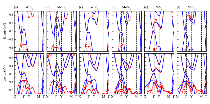
Figure 4: The $I$- and $II$-TB fitted band structures of $MX_{2}$ with SOC. Red dots are first-principles results and black solid lines are fitted TB results. (a-f) Upper panel are the $I$-TB results with SOC; (a-f) Lower panel are the $II$-TB results with SOC.

II.3 Non-trivial topology in $MX_{2}$

The little group of different momenta are always distinct from the space group of the given material. For 1T’-$MX_{2}$, four time-reversal-invariant momenta $\Gamma,\ X,\ Y,$ and $M$ belong to $C_{2h}$, the momenta along two high symmetry lines $X-\Gamma$ and $Y-M$ belong to $C_{2}$, the momenta along $\Gamma-Y$ belong to $C_{s}$, and all the other momenta including those along $\Gamma-M$ belong to a trivial symmetry group with only an identity operation.

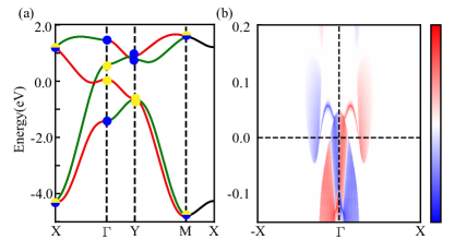
Figure 5: (a) The band structure of monolayer 1T’-WTe₂ along high symmetry lines from the spinless fitted $I$-TB model. Here we denote parities of states at time-reversal invariant momenta with blue and yellow dots and different characters of states along high symmetry lines by red and green lines. (b) Edge spin-polarized density of states along the $\bm{R_{x}}$ direction.

Different from the simple point group symmetry operation, $\bar{M}_{x}$ and $\bar{C}_{2x}$ are associated with a translation operation, thus their detailed matrix representations will depend on the momentum. In the bases of {$\left|\phi_{A,\bm{k}}\right\rangle,\left|\phi_{B,\bm{k}}\right\rangle,\left|\phi_{a,\bm{k}}\right\rangle,\left|\phi_{b,\bm{k}}\right\rangle$}, they are written as

$$\bar{C}_{2x}(k_{x}) =s_{0}\left(\begin{matrix}0&e^{-ik_{x}}\\ 1&0\end{matrix}\right),$$ (3)

$$\bar{M}_{x}(k_{x}) =s_{z}\left(\begin{matrix}1&0\\ 0&e^{-ik_{x}}\end{matrix}\right),$$

$$P =\bar{C}_{2x}(0)\bar{M}_{x}(0).$$

One of the most profound consequences of these non-symmorphic symmetries is that the degeneracy of the states at different momenta might be different even if their momenta belong to the same little group. For example, both $\Gamma$ and $X$ belong to $C_{2h}$, while $\bar{M}_{x}$ can guarantee a double degeneracy at $X$ but not at $\Gamma$. It is because in the sublattice degree of freedom, $\bar{M}_{x}$ is $\tau_{z}$ at $X$, which anti-commutes with $P=\tau_{x}$, while $\bar{M}_{x}$ is $\tau_{0}$ at $\Gamma$, which commutes with $P=\tau_{x}$. Thus, under these symmetry constraints, only $\tau_{0}$ is allowed in Hamiltonian at $X$ leading to the double degeneracy in the sublattice degree of freedom. A similar argument can be applied for the states along $X-M$ where the double degeneracy is protected by $PT$ and $\bar{M}_{x}$ as shown in Fig. 5(a). The two bands around Fermi level along $\Gamma-X$ line belong to different irreducible representations, thus there is a band crossing forming a Dirac cone. With SOC, these two bands will belong to the same representation of the double group, and the band crossing becomes an anti-crossing, leading to a gap opening for the Dirac cone and drives $MX_{2}$ into a 2D topological insulator.

The nontrivial topology can be verified by directly calculating the $Z_{2}$ index using the Fu-Kane formula $(-1)^{\upsilon}=\Pi_{i}\Pi_{m=1}^{N}\xi_{2m}(\Gamma_{i})$, where $N$ is the number of occupied states and $\xi_{2m}(\Gamma_{i})$ is the parity of states at different time-reversal-invariant momentum $\Gamma_{i}$ Choe et al. (2016). In Fig. 5(a), we show the parities for states at four time-reversal-invariant momenta of WTe₂ calculated by our TB model. The $Z_{2}$ index can be easily checked to be 1.

Besides the nonzero $Z_{2}$ topological invariant, we also checked the edge states based on our TB models. As shown in Fig. 5(b), there are two spin-polarized edge states across the band gap connecting the conduction and the valence bands. For a pair of states at different momenta related by the time-reversal symmetry, the spin polarization must be opposite in all directions. For a pair of states at different momenta related by the mirror symmetry $M_{x}$, the $x$-component of spin polarization must be the same. Thus, for the edge states, the spin must be in the $y-z$ plane.(Detail derivation in Appendix C) Our TB models indeed describe these properties correctly as shown in the Fig. 5(b)($z$ component) and Appendix B ($y$ component).

It is worth noting that the underlying mechanism of the nontrivial topology here is exactly the same as the Kane-Mele model for graphene with SOC, where the band inversion happens without SOC and results in two Dirac cones protected by crystalline symmetries, and the SOC opens the band gaps for the Dirac cones to drive the Dirac semimetal into a 2D topological insulator.

III k $\cdot$ p model

Many properties of a fermion system like transport are determined by the states around the Fermi surface. For a semiconductor, the states around the Fermi surface are usually centered around some high-symmetry momenta, and their properties can be described by a simpler $\bm{k\cdot p}$ perturbation model. All the allowed terms in a $\bm{k\cdot p}$ model can be analyzed by considering all the symmetries in the little group of the high-symmetry momentum. Besides, for states belonging to different irreducible representations, the $\bm{k\cdot p}$ models will be different.

Figure 6: Fitted $\bm{k\cdot p}$ model results for $MX_{2}$. (a-f) Red dots are from first-principles calculations and blue solid lines are the fitted $\bm{k\cdot p}$ model results. Green and orange solid dots at $\Gamma$ point represents the even and odd parity, respectively. The fitting region is around $\Gamma$ point and the band inversion momenta.

The space group are the same for all six $MX_{2}$ materials, yet the orbital components around the fermi level are not all identical. At $\Gamma$ point, all six materials present even parity at the valence band maximum (VBM) and different parities at the conduction band minimum (CBM). For $M$Te₂, the CBM parity is even and far away(>0.1 eV) from the next odd parity conduction band. It causes failure to capture symmetry and topological properties if only two same parity bases are considered. Therefore, we also consider the state below VBM and build a three-orbital $\bm{k\cdot p}$ model for $M$Te₂. Specifically, we use {$\left|\phi_{p_{x}},\uparrow\right\rangle,\left|\phi_{p_{x}},\downarrow\right\rangle,\left|\phi_{d_{xz},\uparrow}\right\rangle,\left|\phi_{d_{xz}},\downarrow\right\rangle$} as the bases for $M$Se₂ and $M$S₂, and use {$\left|\phi_{d_{z^{2}}},\uparrow\right\rangle,\left|\phi_{d_{z^{2}}},\downarrow\right\rangle,\left|\phi_{d_{xz}},\uparrow\right\rangle,\left|\phi_{d_{xz}},\downarrow\right\rangle,\left|\phi_{p_{y},\uparrow}\right\rangle,\left|\phi_{p_{y}},\downarrow\right\rangle$} for $M$Te₂ to construct the $\bm{k\cdot p}$ model, respectively.

For $M$Se₂ and $M$S₂, the symmetry operations at $\Gamma$ point are $M_{x}=is_{z}\sigma_{x}$, $P=s_{z}\sigma_{0}$ and time-reversal symmetry operation which reads $T=is_{0}\sigma_{y}K$. For $M$Te₂, symmetry operations at $\Gamma$ point are $P=(\lambda_{0}+2\sqrt{3}\lambda_{8})\sigma_{0}$, $M_{x}=i(\lambda_{0}+3\lambda_{3}-\sqrt{3}\lambda_{8})\sigma_{x}$ and $T=i\lambda_{0}\sigma_{y}K$. $s_{i}$ and $\lambda_{i}$ are Pauli and Gell-Mann matrices for orbital degree of freedom; $\sigma_{i}$ are Pauli matrices for spin degree of freedom and $I_{4/6}$ is an identity matrix. The following Hamiltonian, $H_{1/2}(\bm{k})$ in Eq. 4 are the symmetry-allowed $\bm{k\cdot p}$ models around $\Gamma$ point for $M$Se₂, $M$S₂ and $M$Te₂, respectively (Complete symmetry-allowed terms and detail explanations in Appendix.D).

$$H_{1}(\bm{k}) =\varepsilon_{1}(\bm{k})I_{4}+M_{1}(\bm{k})s_{z}\sigma_{0}+\nu_{1}k_{x}s_{x}\sigma_{y}$$ (4)

$$+\nu_{2}k_{x}s_{x}\sigma_{z},$$

$$H_{2}(\bm{k}) =\varepsilon_{2}(\bm{k})I_{6}+M_{2}(\bm{k})\lambda_{3}\sigma_{0}+M_{3}(\bm{k})\lambda_{8}\sigma_{0}$$

$$+\nu_{1}k_{x}\lambda_{7}\sigma_{0}+\nu_{2}k_{x}\lambda_{4}\sigma_{z},$$

where

$$\varepsilon_{1/2}(\bm{k}) =\mu+t_{x,1}k_{x}^{2}+t_{y,1}k_{y}^{2},$$

$$M_{1/2}(\bm{k}) =\delta+t_{x,2}k_{x}^{2}+t_{y,2}k_{y}^{2},$$

$$M_{3}(\bm{k}) =\delta^{\prime}+t_{x,3}k_{x}^{2}+t_{y,3}k_{y}^{2}.$$

	WTe2	MoTe2	WSe2	MoSe2	WS2	MoS2
$\delta$ (eV)	0.470	0.180	0.342	0.363	0.094	0.239
$\delta^{\prime}$(eV)	0.495	0.443	–	–	–	–
$\mu$ (eV)	0.205	0.086	0.319	0.325	0.051	0.136
$t_{x,1}$ (eV $\cdot$ Å2 )	-7.363	-7.535	-14.814	-12.723	-3.202	-6.826
$t_{y,1}$ (eV $\cdot$ Å2 )	-4.928	-4.656	-3.777	-4.704	-3.732	-2.383
$t_{x,2}$ (eV $\cdot$ Å2 )	-7.207	-5.756	-16.107	-14.148	-5.869	-9.644
$t_{y,2}$ (eV $\cdot$ Å2 )	-0.184	0.519	1.137	-0.149	7.269	3.414
$t_{x,3}$ (eV $\cdot$ Å2 )	-7.996	-8.665	–	–	–	–
$t_{y,3}$ (eV $\cdot$ Å2 )	-3.223	-3.282	–	–	–	–
$\nu_{1}$ (eV $\cdot$ Å)	0.699	1.157	0.168	0.343	0.387	0.337
$\nu_{2}$ (eV $\cdot$ Å)	0.349	0.358	0.333	0.343	0.482	0.153

Table 4: Fitted $\bm{k\cdot p}$ model parameters for all six $MX_{2}$.

In Eq. 4, we only keep $k_{i}^{2}$($i=x,y$) in the mass dependent terms and $k_{i}$ in the velocity terms. The positive $\delta$ and $\delta^{\prime}$ represent the band inversion nature at $\Gamma$ point. Without SOC, the band crossing only occurs along $X$ - $\Gamma$, thus we ignore $k_{y}$ terms in the $\bm{k\cdot p}$ model. In this sense, our $\bm{k\cdot p}$ model at least can capture the band shape and the orbital reordering nature.

The $\bm{k\cdot p}$ model for $M$Te₂ reveals the interplays between three orbitals and provides another angle to understand the semimetallic properties of $M$Te₂. In TABLE 4, the $t_{x}$ terms are much larger than the $t_{y}$ terms, suggesting a strong anisotropy in momentum space. It is also found that by fine tuning the SOC strength, a positive gap opens and the gap value shows a monotonic relationship with the SOC strength. In the next section, we discuss a strained TB model, where the strain effects are reflected in the hopping parameters.

IV STRAINED TB MODEL

Strain is one of the most important approaches to tune the electronic properties of 2D materials. Experimental results prove the strain can induce metal-insulator transition and enhance the metastable phase growthChen et al. (2021); Zhao et al. (2020). In this section, we introduce the strained TB model based on the $I$-TB model.

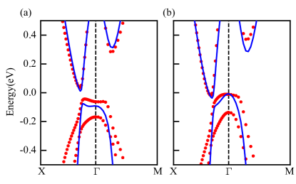
Figure 7: The Band structures from first-principles calculations and strained TB model. (a) and (b) are WTe₂ band structures under a 5% tensile strain along the $\bm{R_{x}}$ direction and under a compressive strain along the $\bm{R_{y}}$ direction, respectively. All the first-principles calculation results and strained TB model results are labeled by red dots and blue lines, respectively.

Assuming that a small uniaxial strain (around $\pm$ 1.0%) is applied to $MX_{2}$ without breaking any symmetries, we consider the strain as a small perturbation and only change the overlap between different orbitals. In the strained TB model, the strain effects on band structures are captured by changing the hopping parameters. Then a series of linear fittings are conducted within a small range of strain using Eq. 5:

$$t^{\prime}(r_{ix}(1+\Delta_{x}|\bm{R_{x}}|),r_{iy}) =\sum_{j=0}a_{x,j}\Delta_{x}^{j},$$ (5)

$$t^{\prime}(r_{ix},r_{iy}(1+\Delta_{y}|\bm{R_{y}}|)) =\sum_{j=0}a_{y,j}\Delta_{y}^{j}.$$

Here, only a uniaxial strain is included. $a_{x/y,j}$ represents the $j^{th}$ order polynomial coefficient in the $x/y$ direction and $\Delta_{x/y}$ is the strain strength.

$a_{x,1}(t_{1})$	$a_{x,0}(t_{1})$	$a_{x,1}(d_{1})$	$a_{x,0}(d_{1})$	$a_{x,1}(p_{1})$	$a_{x,0}(p_{1})$	$a_{x,1}(p_{2})$	$a_{x,0}(p_{2})$
$a_{y,1}(t_{1})$	$a_{y,0}(t_{1})$	$a_{y,1}(d_{1})$	$a_{y,0}(d_{1})$	$a_{y,1}(p_{1})$	$a_{y,0}(p_{1})$	$a_{y,1}(p_{2})$	$a_{y,0}(p_{2})$
-3.059	1.019	-1.467	0.468	-2.207	1.063	-2.798	0.374
4.823	1.015	0.330	0.461	2.777	1.068	4.225	0.376

Table 5: Fitted parameters for WTe₂ strained TB model.

In Fig. 7, we present the band structures of 1T’-WTe₂ under uniaxial strain along the $\bm{R_{x}}$ and the $\bm{R_{y}}$ directions, respectively. Our strained TB model results for 1T’-WTe₂ are based on Eq. 5 to the linear order which are consistent with the first-principles calculations up to  5% strain strength. The strain effects along different direction are not identical. To be more specific, it is the tensile strain along the $x$ direction or the compressive strain along the $y$ direction that contributes to a more positive fundamental gap. Our strained TB model also reflects this strain anisotropy: in TABLE 5, most linear order parameters have different signs along different directions. Besides, we believe the bulk conductance of all six $MX_{2}$ materials can be easily manipulated by external strain due to the similar orbital components and dispersions. Our strained TB model serves as a suitable starting point to analyze the electronic properties of $MX_{2}$ under perturbations.

In Appendix E, we provide the insulating 1T’-WTe₂ nontrivial edge density of states under strong enough uniaxial strain. This shows that the strain does not only open a fundamental gap in $MX_{2}$, but also preserves the nontrivial topology.

V SUMMARY

In this paper, we constructed four-band TB models based on the orbital components of monolayer 1T’-$MX_{2}$ . By analyzing the nonsymmorphic space group of 1T’-$MX_{2}$ structure, bases from $A_{g}$ and $A_{u}$ IRs in $C_{2h}$ were selected. Our TB models match well with the first-principles band structures along all high symmetric lines. $I$-TB model with fewer parameters fits well within the energy window from -0.3 eV to 0.3 eV; $II$-TB model with more parameters fits well within the energy window from -0.3 eV to 0.8 eV. With the inclusion of SOC effects, both TB models can capture the nontrivial topological properties of 1T’-$MX_{2}$. Specifically, we find that the momenta belong to the same little group have different degeneracies due to features of the nonsymmorphic group. Plus, the spin of edge states along the $\bm{R_{x}}$ direction always lies in the $y-z$ plane, which is guaranteed by the time-reversal symmetry and the mirror symmetry $M_{x}$. Moreover, for the first time, we found that $MX_{2}$ have different parities at $\Gamma$ point, and then we built two different types of $\bm{k\cdot p}$ model to fully describe the low-energy properties of $MX_{2}$. In the last section, we built the strained TB model to capture the effects of uniaxial strain along $\bm{R_{x}}$ and $\bm{R_{y}}$. The small tensile strain along the $x$ direction or compressive strain along the $y$ direction induces a metal-insulator transition. To conclude, our TB and $\bm{k\cdot p}$ models are simple and efficient to describe the 1T’-$MX_{2}$ band structure and its topological properties, which can serve as a solid foundation for future studies of superconductivity and other many-body physics in 1T’-$MX_{2}$.

VI ACKNOWLEDGMENTS

We thank Vic K. T. Law, Jason Z.S. Gao, and Noah F.Q. Yuan for helpful discussions. This work is supported by the Research Grants Council of Hong Kong (ECS26302118,16305019, 16306220 and N_HKUST626/18) and National Natural Science Foundation of China (NSFC20SC07).

Appendix A Appendix A: Layout of Tight-binding parameters

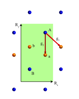
Figure 8: Top view of the reduced lattice structure of monolayer $MX_{2}$. $M$ atom is in blue and $X_{1}$ atom is in orange. Unit cell is labeled by the green rectangle. Two basic vectors are labeled as $\bm{g_{1}}$and $\bm{g_{2}}$ to be accounted for generating other $\bm{r_{i}}$. The unit vectors are labeled as $\bm{R_{x}}$ and $\bm{R_{y}}$

We label all the hoppings in real space included in our TB model with the following notations.

$$\bm{r^{dp}_{1}}=\bm{g_{1}}, \bm{r^{dp}_{2}} =\bm{g_{2}}+\bm{R_{x}}$$

$$\bm{r^{dp}_{3}}=\bm{g_{1}}+\bm{R_{x}}+\bm{R_{y}}, \bm{r^{dp}_{4}} =\bm{g_{2}}+\bm{R_{x}}+\bm{R_{y}}$$

$$\bm{r^{dp}_{5}}=\bm{g_{2}}+\bm{R_{x}}-\bm{R_{y}}, \bm{r^{dp}_{6}} =\bm{g_{1}}+\bm{R_{x}}-\bm{R_{y}}$$

$$\bm{r^{pp}_{1}}=\bm{R_{x}}, \bm{r^{pp}_{2}} =\bm{g_{1}}-\bm{g_{2}}$$

$$\bm{r^{pp}_{3}}=\bm{R_{y}}, \bm{r^{pp}_{4}} =\bm{g_{1}}-\bm{g_{2}}-\bm{R_{y}}$$

$$\bm{r^{pp}_{5}}=\bm{g_{1}}-\bm{g_{2}}+\bm{R_{y}}, \bm{r^{pp}_{6}} =\bm{R_{x}}+\bm{R_{y}}$$

$$\bm{r^{dd}_{1}}=\bm{g_{1}}+\bm{g_{2}}+\bm{R_{y}}, \bm{r^{dd}_{2}} =\bm{R_{x}}$$

$$\bm{r^{dd}_{3}}=\bm{g_{1}}+\bm{g_{2}}, \bm{r^{dd}_{4}} =\bm{R_{y}}$$

$$\bm{r^{dd}_{5}}=\bm{R_{x}}+\bm{R_{y}}, \bm{r^{dd}_{6}} =\bm{g_{1}}+\bm{g_{2}}-\bm{R_{y}}$$

The hopping parameters in the main text are defined as

$$t_{i}(\bm{r^{dp}_{i}}) =\left\langle\phi_{l}(\bm{r})\middle|\hat{H}\middle|\phi_{l^{\prime}}(\bm{r-r^{dp}_{i}})\right\rangle;$$

$$d_{i}(\bm{r^{dd}_{i}}) =\left\langle\phi_{l}(\bm{r})\middle|\hat{H}\middle|\phi_{l^{\prime}}(\bm{r-r^{dd}_{i}})\right\rangle;$$

$$p_{i}(\bm{r^{pp}_{i}}) =\left\langle\phi_{l}(\bm{r})\middle|\hat{H}\middle|\phi_{l^{\prime}}(\bm{r-r^{pp}_{i}})\right\rangle(l,l^{\prime}=A,B,a,b).$$

The symmetry constraints of the hopping parameters read:

$$t_{i}(\bm{r^{dp}_{i}})= -t_{i}(M_{x}\bm{r^{dp}_{i}})= -t_{i}(P\bm{r^{dp}_{i}})$$ (6)

$$d_{i}(\bm{r^{dd}_{i}})= \ d_{i}(M_{x}\bm{r^{dp}_{i}})= \ d_{i}(P\bm{r^{dd}_{i}})$$

$$p_{i}(\bm{r^{dd}_{i}})= \ p_{i}(M_{x}\bm{r^{dp}_{i}})= \ p_{i}(P\bm{r^{dd}_{i}})$$

Similarly, we consider the symmetry constraints in the SOC terms. In the main text, only $\bm{g_{1}},\ \bm{g_{2}}$ connected off-site SOC terms are constructed. We label the SOC parameters as: $il_{j}(\bm{g_{j}})=\left\langle\phi_{A/B,\alpha}(\bm{r})\middle|\hat{H}\middle|\phi_{a/b,\alpha^{\prime}}(\bm{r-g_{j}})\right\rangle$, ($\alpha,\alpha^{\prime}=\uparrow,\downarrow$).

Since the $M_{x}$ operation anti-commutes with $\sigma_{y}$ and $\sigma_{z}$ in spin bases, we consider the SOC effects in the $y$ and the $z$ directions. The symmetry constraints to the SOC parameters read:

$$il_{j}(\bm{g_{1}})=\ il_{j}(M_{x}\bm{g_{1}}) =-il_{j}(P\bm{g_{1}})$$ (7)

$$il_{j}(\bm{g_{2}})=-il_{j}(P\bm{g_{2}})$$

Appendix B: Edge density of states

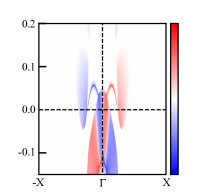
Figure 9: WTe₂ edge spin-polarized density of states in the $y$ direction.

In the main-text, spin-polarized density of states in the $z$ direction is presented. Here we supplement the result in the $y$ direction.

Appendix C: Symmetry-protected degeneracy and zero spin polarization

For any lattice structure which preserves time-reversal ($T$) and inversion ($P$) symmetries, the Hamiltonian satisfies the constraints:

$$=[H,P]=0$$ (8)

$$H\left|k_{i},\sigma_{i}\right\rangle =E\left|k_{i},\sigma_{i}\right\rangle$$

where $\left|k_{i},\sigma_{i}\right\rangle$ is the eigenstate of $H$, we apply the symmetry operations ($T,P$) on both sides of the equation:

$$TH\left|k_{i},\sigma_{i}\right\rangle =ET\left|k_{i},\sigma_{i}\right\rangle$$ (9)

$$PH\left|k_{i},\sigma_{i}\right\rangle =EP\left|k_{i},\sigma_{i}\right\rangle$$

$$\text{with}\eqref{eq:1},$$

$$TH\left|k_{i},\sigma_{i}\right\rangle =HT\left|k_{i},\sigma_{i}\right\rangle$$

$$PH\left|k_{i},\sigma_{i}\right\rangle =HP\left|k_{i},\sigma_{i}\right\rangle$$

now for every eigenvalue $E$, we have at most two eigenstates labeled by different spin vectors:

$$T\left|k_{i},\sigma_{i}\right\rangle =\left|-k_{i},-\sigma_{i}\right\rangle$$ (10)

$$P\left|k_{i},\sigma_{i}\right\rangle =\left|-k_{i},\sigma_{i}\right\rangle$$

Here, we denote the eigenstates by momentum and spin polarization ($\left|k_{i},\sigma_{i}\right\rangle,\ (i=x,y,z)$). For any spin polarization direction, if $\sigma_{i}$ is not zero, we can always find the spin symmetry ‘partner’ ($-\sigma_{i}$) and the summation of every spin partner ($\rho(E,k_{i})_{i}$) is zero; if $\sigma_{i}$ is zero, it will directly contribute to the zero spin density of states. With a similar deduction process, when the edge structure only preserves mirror ($M$) and time-reversal symmetries, since mirror symmetry operator ($M_{i}=i\sigma_{i}$) commute with $\sigma_{i}$, the spin symmetry ‘partner’ ($-\sigma_{i}$) can only be found along the $i$ direction. To summarize, the zero $\rho(E,k_{i})_{i}$ protected by the combination of time-reversal symmetry and one crystalline symmetry whose operator commute with $\sigma_{i}$.

Appendix D: symmetry constraints of the k$\cdot$p model

We use the bases {$\left|\phi_{p_{x}},\uparrow\right\rangle,\left|\phi_{p_{x}},\downarrow\right\rangle,\left|\phi_{d_{xz},\uparrow}\right\rangle,$$\left|\phi_{d_{xz}},\downarrow\right\rangle$} for $M$Se₂, $M$S₂ and {$\left|\phi_{d_{z^{2}}},\uparrow\right\rangle,\left|\phi_{d_{z^{2}}},\downarrow\right\rangle,\left|\phi_{d_{xz}},\uparrow\right\rangle,\left|\phi_{d_{xz}},\downarrow\right\rangle,$ $\left|\phi_{p_{y},\uparrow}\right\rangle,\left|\phi_{p_{y}},\downarrow\right\rangle$} for $M$Te₂.

Symmetry operations at $\Gamma$ point are $M_{x}=is_{z}\sigma_{x}$, $P=s_{z}\sigma_{0}$, and $T=is_{0}\sigma_{y}K$ for $M$Se₂ and $M$S₂, and $P=(\lambda_{0}+2\sqrt{3}\lambda_{8})\sigma_{0}$, $M_{x}=i(\lambda_{0}+3\lambda_{3}-\sqrt{3}\lambda_{8})\sigma_{x}$ and $T=i\lambda_{0}\sigma_{y}K$ for $M$Te₂. The following table lists the symmetry transformation relationships under different $k_{i}$, $s_{i}\sigma_{j}$, and $\lambda_{i}\sigma_{j}$.

$P$	$M_{x}$	$T$	$\bm{k}$	$s_{i}\sigma_{i}$	$\lambda_{i}\sigma_{i}$
+1	+1	+1	1;$k_{x}^{2}$;$k_{y}^{2}$	$s_{0/z}\sigma_{0}$	$\lambda_{3/8}\sigma_{0}$ ;$\lambda_{2}\sigma_{y/z}$
+1	+1	-1	–	$s_{0/z}\sigma_{x}$	$\lambda_{3/8}\sigma_{x}$ ;$\lambda_{1}\sigma_{y/z}$
+1	-1	+1	$k_{x}k_{y}$	–	$\lambda_{1}\sigma_{0}$;$\lambda_{2}\sigma_{x}$
-1	+1	+1	–	$s_{x}\sigma_{0}$ ; $s_{y}\sigma_{x}$	$\lambda_{4}\sigma_{0}$;$\lambda_{5}\sigma_{x}$;$\lambda_{7}\sigma_{y/z}$
+1	-1	-1	–	$s_{0/z}\sigma_{y/z}$	$\lambda_{2}\sigma_{0}$;$\lambda_{1}\sigma_{x}$;$\lambda_{3/8}\sigma_{y/z}$
-1	+1	-1	$k_{y}$	$s_{x}\sigma_{x}$ ; $s_{y}\sigma_{0}$	$\lambda_{5}\sigma_{0}$;$\lambda_{4}\sigma_{x}$;$\lambda_{6}\sigma_{y/z}$
-1	-1	+1	–	$s_{y}\sigma_{y/z}$	$\lambda_{6}\sigma_{0}$;$\lambda_{7}\sigma_{x}$;$\lambda_{5}\sigma_{y/z}$
-1	-1	-1	$k_{x}$	$s_{x}\sigma_{y/z}$	$\lambda_{7}\sigma_{0}$;$\lambda_{6}\sigma_{x}$;$\lambda_{4}\sigma_{y/z}$

Table 6: The character table for the $\bm{k\cdot p}$ models.

The symmetry-allowed terms in the $\bm{k\cdot p}$ model read:

$$H_{1}(\bm{k}) =\epsilon_{1}(\bm{k})I_{4}+M_{1}(\bm{k})s_{z}\sigma_{0}+\nu_{1}k_{x}s_{x}\sigma_{y}+\nu_{2}k_{x}s_{x}\sigma_{z}$$ (11)

$$+\nu_{3}k_{y}s_{x}\sigma_{x}+\nu_{4}k_{y}s_{y}\sigma_{0}$$

$$H_{2}(\bm{k}) =\epsilon_{2}(\bm{k})I_{6}+M_{1}(\bm{k})\lambda_{3}\sigma_{0}+M_{2}(\bm{k})\lambda_{8}\sigma_{0}$$

$$+M_{3}(\bm{k})\lambda_{2}\sigma_{y}+M_{4}(\bm{k})\lambda_{2}\sigma_{z}+\nu_{1}k_{x}\lambda_{7}\sigma_{0}$$

$$+\nu_{2}k_{x}\lambda_{4}\sigma_{z}+\nu_{3}k_{x}\lambda_{4}\sigma_{y}+\nu_{4}k_{x}\lambda_{6}\sigma_{x}$$

$$+\nu_{5}k_{y}\lambda_{5}\sigma_{0}+\nu_{6}k_{y}\lambda_{4}\sigma_{x}+\nu_{7}k_{y}\lambda_{6}\sigma_{y}$$

$$+\nu_{8}k_{y}\lambda_{6}\sigma_{z}$$

$$\epsilon_{1/2}(\bm{k}) =\mu+t_{x,1}k_{x}^{2}+t_{y,1}k_{y}^{2}$$

$$M_{1}(\bm{k}) =-\delta+t_{x,2}k_{x}^{2}+t_{y,2}k_{y}^{2}$$

$$M_{2}(\bm{k}) =-\delta^{\prime}+t_{x,3}k_{x}^{2}+t_{y,3}k_{y}^{2}$$

$$M_{3}(\bm{k}) =-\delta_{3}+t_{x,4}k_{x}^{2}+t_{y,4}k_{y}^{2}$$

$$M_{4}(\bm{k}) =-\delta_{4}+t_{x,5}k_{x}^{2}+t_{y,5}k_{y}^{2}$$

In Eq. 11 we list all the symmetry-allowed terms up to $k_{i}^{2}$ ($i=x,y$). In the main text, only $\epsilon_{1/2}$, $M(\bm{k})_{1/2}$, and $\nu_{1/2}$ are included.

Appendix E: Edge density of states from strained TB model

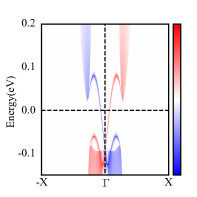
Figure 10: WTe₂ edge spin-polarized density of states in the $y$ direction. The strained TB parameters are under 5% tensile strain along $\bm{R_{x}}$ direction.

References

- Kane and Mele (2005) C. L. Kane and E. J. Mele, Phys. Rev. Lett. 95, 226801 (2005).
- Hasan and Kane (2010) M. Z. Hasan and C. L. Kane, Rev. Mod. Phys. 82, 3045 (2010).
- Qi and Zhang (2011) X.-L. Qi and S.-C. Zhang, Rev. Mod. Phys. 83, 1057 (2011).
- Bansil et al. (2016) A. Bansil, H. Lin, and T. Das, Rev. Mod. Phys. 88, 021004 (2016).
- Bernevig et al. (2006) B. A. Bernevig, T. L. Hughes, and S.-C. Zhang, Science 314, 1757 (2006).
- König et al. (2007) M. König, S. Wiedmann, C. Brüne, A. Roth, H. Buhmann, L. W. Molenkamp, X.-L. Qi, and S.-C. Zhang, Science 318, 766 (2007).
- Liu et al. (2008) C. Liu, T. L. Hughes, X.-L. Qi, K. Wang, and S.-C. Zhang, Phys. Rev. Lett. 100, 236601 (2008).
- Knez et al. (2011) I. Knez, R.-R. Du, and G. Sullivan, Phys. Rev. Lett. 107, 136603 (2011).
- Qian et al. (2014) X. Qian, J. Liu, L. Fu, and J. Li, Science 346, 1344 (2014).
- Fei et al. (2017) Z. Fei, T. Palomaki, S. Wu, W. Zhao, X. Cai, B. Sun, P. Nguyen, J. Finney, X. Xu, and D. H. Cobden, Nat. Phys. 13, 677 (2017).
- Wu et al. (2018) S. Wu, V. Fatemi, Q. D. Gibson, K. Watanabe, T. Taniguchi, R. J. Cava, and P. Jarillo-Herrero, Science 359, 76 (2018).
- Tang et al. (2017a) S. Tang, C. Zhang, D. Wong, Z. Pedramrazi, H.-Z. Tsai, C. Jia, B. Moritz, M. Claassen, H. Ryu, S. Kahn, et al., Nat. Phys. 13, 683 (2017a).
- Peng et al. (2017) L. Peng, Y. Yuan, G. Li, X. Yang, J.-J. Xian, C.-J. Yi, Y.-G. Shi, and Y.-S. Fu, Nat. Commun. 8, 1 (2017).
- Jia et al. (2017) Z.-Y. Jia, Y.-H. Song, X.-B. Li, K. Ran, P. Lu, H.-J. Zheng, X.-Y. Zhu, Z.-Q. Shi, J. Sun, J. Wen, et al., Phys. Rev. B 96, 041108 (2017).
- Palomaki et al. (2018) T. Palomaki, X. Xu, S. Luescher, C. Olsen, W. Zhao, Z. Fei, D. H. Cobden, J. A. Folk, P. Bement, and E. Sajadi, Science 362, 922 (2018).
- Fatemi et al. (2018) V. Fatemi, S. Wu, Y. Cao, L. Bretheau, Q. D. Gibson, K. Watanabe, T. Taniguchi, R. J. Cava, and P. Jarillo-Herrero, Science 362, 926 (2018).
- Hsu et al. (2020) Y.-T. Hsu, W. S. Cole, R.-X. Zhang, and J. D. Sau, Phys. Rev. Lett. 125, 097001 (2020).
- Xie et al. (2020) Y.-M. Xie, B. T. Zhou, and K. Law, Phys. Rev. Lett. 125, 107001 (2020).
- Fei et al. (2018) Z. Fei, W. Zhao, T. A. Palomaki, B. Sun, M. K. Miller, Z. Zhao, J. Yan, X. Xu, and D. H. Cobden, Nature 560, 336 (2018).
- Sharma et al. (2019) P. Sharma, F.-X. Xiang, D.-F. Shao, D. Zhang, E. Y. Tsymbal, A. R. Hamilton, and J. Seidel, Sci. Adv. 5, eaax5080 (2019).
- Soluyanov et al. (2015) A. A. Soluyanov, D. Gresch, Z. Wang, Q. Wu, M. Troyer, X. Dai, and B. A. Bernevig, Nature 527, 495 (2015).
- Xu et al. (2018a) S. Y. Xu, Q. Ma, H. Shen, V. Fatemi, S. Wu, T. R. Chang, G. Chang, A. M. Valdivia, C. K. Chan, Q. D. Gibson, J. Zhou, Z. Liu, K. Watanabe, T. Taniguchi, H. Lin, R. J. Cava, L. Fu, N. Gedik, and P. Jarillo-Herrero, Nat. Phys. 14, 900 (2018a).
- MacNeill et al. (2017) D. MacNeill, G. M. Stiehl, M. H. Guimaraes, R. A. Buhrman, J. Park, and D. C. Ralph, Nat. Phys. 13, 300 (2017).
- Wu et al. (2015) Y. Wu, N. H. Jo, M. Ochi, L. Huang, D. Mou, S. L. Bud’ko, P. C. Canfield, N. Trivedi, R. Arita, and A. Kaminski, Phys. Rev. Lett. 115, 166602 (2015).
- Pan et al. (2015) X.-C. Pan, X. Chen, H. Liu, Y. Feng, Z. Wei, Y. Zhou, Z. Chi, L. Pi, F. Yen, F. Song, et al., Nat. Commun. 6, 7805 (2015).
- Kang et al. (2015) D. Kang, Y. Zhou, W. Yi, C. Yang, J. Guo, Y. Shi, S. Zhang, Z. Wang, C. Zhang, S. Jiang, et al., Nat. Commun. 6, 7804 (2015).
- Chen et al. (2018) P. Chen, W. W. Pai, Y.-H. Chan, W.-L. Sun, C.-Z. Xu, D.-S. Lin, M. Chou, A.-V. Fedorov, and T.-C. Chiang, Nat. Commun. 9 (2018), 10.1038/s41467-018-04395-2.
- Pedramrazi et al. (2019) Z. Pedramrazi, C. Herbig, A. Pulkin, S. Tang, M. Phillips, D. Wong, H. Ryu, M. Pizzochero, Y. Chen, F. Wang, et al., Nano letters 19, 5634 (2019).
- Chen et al. (2021) W. Chen, M. Hu, J. Zong, X. Xie, Q. Meng, F. Yu, L. Wang, W. Ren, A. Chen, G. Liu, et al., Advanced Materials 33, 2004930 (2021).
- Cheng et al. (2019) F. Cheng, Z. Hu, H. Xu, Y. Shao, J. Su, Z. Chen, W. Ji, and K. P. Loh, ACS nano 13, 2316 (2019).
- Naylor et al. (2016) C. H. Naylor, W. M. Parkin, J. Ping, Z. Gao, Y. R. Zhou, Y. Kim, F. Streller, R. W. Carpick, A. M. Rappe, M. Drndic, et al., Nano letters 16, 4297 (2016).
- Xu et al. (2018b) H. Xu, D. Han, Y. Bao, F. Cheng, Z. Ding, S. J. Tan, and K. P. Loh, Nano Lett. 18, 5085 (2018b).
- Deng et al. (2016) K. Deng, G. Wan, P. Deng, K. Zhang, S. Ding, E. Wang, M. Yan, H. Huang, H. Zhang, Z. Xu, et al., Nat. Phys. 12, 1105 (2016).
- Qi et al. (2016) Y. Qi, P. G. Naumov, M. N. Ali, C. R. Rajamathi, W. Schnelle, O. Barkalov, M. Hanfland, S. C. Wu, C. Shekhar, Y. Sun, V. Süß, M. Schmidt, U. Schwarz, E. Pippel, P. Werner, R. Hillebrand, T. Förster, E. Kampert, S. Parkin, R. J. Cava, C. Felser, B. Yan, and S. A. Medvedev, Nat. Commun. 7, 1 (2016).
- Tang et al. (2017b) S. Tang, C. Zhang, D. Wong, Z. Pedramrazi, H.-Z. Tsai, C. Jia, B. Moritz, M. Claassen, H. Ryu, S. Kahn, J. Jiang, H. Yan, M. Hashimoto, D. Lu, R. G. Moore, C.-C. Hwang, C. Hwang, Z. Hussain, Y. Chen, M. M. Ugeda, Z. Liu, X. Xie, T. P. Devereaux, M. F. Crommie, S.-K. Mo, and Z.-X. Shen, Nat. Phys. 13, 683 (2017b).
- Song et al. (2018) Y.-H. Song, Z.-Y. Jia, D. Zhang, X.-Y. Zhu, Z.-Q. Shi, H. Wang, L. Zhu, Q.-Q. Yuan, H. Zhang, D.-Y. Xing, et al., Nat. Commun. 9, 1 (2018).
- Muechler et al. (2016) L. Muechler, A. Alexandradinata, T. Neupert, and R. Car, Phys. Rev. X 6, 041069 (2016).
- Ok et al. (2019) S. Ok, L. Muechler, D. Di Sante, G. Sangiovanni, R. Thomale, and T. Neupert, Phys. Rev. B 99, 121105(R) (2019).
- Choe et al. (2016) D.-H. Choe, H.-J. Sung, and K. J. Chang, Phys. Rev. B 93, 125109 (2016).
- Kresse and Furthmüller (1996) G. Kresse and J. Furthmüller, Comput. Mater. Sci. 6, 15 (1996).
- Blöchl (1994) P. E. Blöchl, Phys. Rev. B 50, 17953 (1994).
- Perdew et al. (1996) J. P. Perdew, K. Burke, and M. Ernzerhof, Phys. Rev. Lett. 77, 3865 (1996).
- Zhao et al. (2020) C. Zhao, M. Hu, J. Qin, B. Xia, C. Liu, S. Wang, D. Guan, Y. Li, H. Zheng, J. Liu, et al., Physical Review Letters 125, 046801 (2020).