The EM Algorithm is Adaptively-Optimal for Unbalanced Symmetric Gaussian Mixtures

Abstract

This paper studies the problem of estimating the means $\pm\theta_{*}\in\mathbb{R}^{d}$ of a symmetric two-component Gaussian mixture $\delta_{*}\cdot N(\theta_{*},I)+(1-\delta_{*})\cdot N(-\theta_{*},I)$ where the weights $\delta_{*}$ and $1-\delta_{*}$ are unequal. Assuming that $\delta_{*}$ is known, we show that the population version of the EM algorithm globally converges if the initial estimate has non-negative inner product with the mean of the larger weight component. This can be achieved by the trivial initialization $\theta_{0}=0$. For the empirical iteration based on $n$ samples, we show that when initialized at $\theta_{0}=0$, the EM algorithm adaptively achieves the minimax error rate $\tilde{O}\Big{(}\min\Big{\{}\frac{1}{(1-2\delta_{*})}\sqrt{\frac{d}{n}},\frac{1}{\|\theta_{*}\|}\sqrt{\frac{d}{n}},\left(\frac{d}{n}\right)^{1/4}\Big{\}}\Big{)}$ in no more than $O\Big{(}\frac{1}{\|\theta_{*}\|(1-2\delta_{*})}\Big{)}$ iterations (with high probability). We also consider the EM iteration for estimating the weight $\delta_{*}$, assuming a fixed mean $\theta$ (which is possibly mismatched to $\theta_{*}$). For the empirical iteration of $n$ samples, we show that the minimax error rate $\tilde{O}\Big{(}\frac{1}{\|\theta_{*}\|}\sqrt{\frac{d}{n}}\Big{)}$ is achieved in no more than $O\Big{(}\frac{1}{\|\theta_{*}\|^{2}}\Big{)}$ iterations. These results robustify and complement recent results of Wu and Zhou [38] obtained for the equal weights case $\delta_{*}=1/2$.

1 Introduction

The expectation-maximization (EM) algorithm is a heuristic formulated in [9] to approximate the maximum likelihood estimator (MLE) in parametric models $(X,S)\sim P_{\theta}(x,s)$ when $X$ is observed, but $S$ is latent. Remarkably, despite its simplicity, widespread use, and rich history [27, 14], no theoretical guarantees on its performance for finite number of iterations and samples were established until recently. The first such explicit guarantees were obtained in [3], which stated general bounds on the statistical precision, the convergence rate, and the “basin of attraction” (the distance of the initial estimate from the ground truth sufficient to obtain a statistically accurate solution). These bounds apply to any latent variables model, yet require verifying several conditions for each concrete model. As a canonical example, these conditions were explicitly verified by [3] for the symmetric two-component Gaussian mixture (2-GM). The resulting guarantees are not sharp, however, both in the strong conditions required for their validity, as well as their distance from the accuracy guarantees of optimal algorithms. Consequently, a dedicated analysis of EM for 2-GM was conducted by various authors [23, 36, 39, 8, 38, 10, 12, 11]. The performance of EM for 2-GM with balanced components, i.e., when both weights equal $1/2$, was by and large recently settled in [38].

In this paper, we proceed in the direction of [38], and sharply analyze a slight variation of the balanced 2-GM model – namely, the unbalanced symmetric 2-GM model. Some of the key arguments in [38] strongly depend on the symmetry properties of the EM iteration, which are a direct result of the symmetry in the model. It seems challenging to adapt these arguments to the unbalanced model, where symmetry breaks down due to the unequal weights. Our analysis therefore uses indirect arguments, which are based on comparisons between the EM iterations of unbalanced models for different weights. In particular, we compare the iterations for unbalanced models with the iterations for the balanced model, since the latter is already known to globally converge [38]. For the population iteration, we prove that increasing the larger of the two weights, that is, enhancing the model imbalance, makes the corresponding EM iteration converge faster. By contrast, this increase also increases our empirical error bound, i.e., the bound on the difference between the empirical iteration and the population iteration. As we prove, however, this does not result in deterioration of the statistical accuracy of the estimate because this increased error is compensated for by the improved convergence of the population iteration. Hence, the overall statistical accuracy actually improves when the model is more unbalanced.

1.1 EM for two-component Gaussian mixture

The symmetric two-component Gaussian mixture (2-GM) model in $d\geqslant 1$ dimensions is given by

$$P_{\theta,\rho}=\tfrac{1+\rho}{2}\cdot N(\theta,I_{d})+\tfrac{1-\rho}{2}\cdot N(-\theta,I_{d})\,.$$ (1)

The goal is to estimate the parameter $\theta_{*}\in\mathbb{R}^{d}$ from $n$ samples $(X_{1},\ldots,X_{n})\stackrel{{\scriptstyle\tiny\mathrm{i.i.d.}}}{{\sim}}P_{\theta_{*},\rho_{*}}$ under the $\ell_{2}$ loss function $\ell(\theta,\theta_{*})=\|\theta-\theta_{*}\|$ when $\rho_{*}\neq 0$ (unbalanced model), or under $\ell_{0}(\theta,\theta_{*})=\min(\|\theta-\theta_{*}\|,\|\theta+\theta_{*}\|)$ when $\rho_{*}=0$ (balanced model). The dimension $d$ is allowed to be large, and both $d$ and $\rho_{*}$ may scale with the number of samples $n$. Based on the $n$ samples and the value of $\rho_{*}$, the EM algorithm defines a mapping $f_{n}(\theta)$ which is iteratively applied to produce a sequence of estimates $\theta_{t}=f_{n}(\theta_{t-1})$ for all $t\geqslant 1$, given an initial guess $\theta_{0}$. This mapping $f_{n}$ is described in detail later in the introduction. We will refer to $f_{n}(\theta)$ as the empirical iteration, and to the idealized operator $f(\theta)$ obtained by replacing empirical averages with expected values as the population iteration.

Balanced GM.

The general results of [3] specialized to the balanced 2-GM (1) ($\rho_{*}=0$) require that the separation between the means is lower bounded as $\|\theta_{*}\|=\Omega(1)$, and that the initial estimate $\theta_{0}$ is at most $\|\theta_{*}\|/4$ in $\ell_{2}$ distance from $\theta_{*}$. When these two conditions hold, [3] states that EM converges to a neighborhood of $\theta_{*}$ of radius $O(\sqrt{d/n})$ (i.e., parametric error rate), after no more than $O(1/\|\theta_{*}\|^{2})$ iterations. The qualifying conditions above are problematic for several reasons: (1) Without knowing $\theta^{*}$ one has no way of knowing when the separation condition holds; (2) EM can be slow and inaccurate when there is no separation between the components [29] and in this case no guarantees are provided by [3]; (3) One of the main challenges in utilizing EM is the choice of initial guess. A common method is attempting multiple random guesses [22] followed by a choice of the optimal converged solution. For a high-dimensional parameter, the guarantee of [3] on the volume of the basin of attraction that ensures good convergence is negligible compared to the volume of the feasible set of parameters, and hence randomly initializing is not proved to succeed.

These drawbacks have lead to various attempts to sharpen the above results [23, 36, 39, 8, 38], which will be discussed in more detail in Section 1.5. For the population iteration, the papers [39, 8, 38] proved global convergence to $\pm\theta_{*}$ at a geometric rate, unless the initial guess $\theta_{0}$ is orthogonal to $\theta_{*}$ (in which case EM converges to the saddle point $\theta=0$). For the empirical iteration, sharp high-probability guarantees were obtained in [38] as follows: In the worst case, without any separation condition, the EM algorithm applied to (1) achieves an error rate of $\tilde{O}((d/n)^{1/4})$ in at most $O(\sqrt{n})$ iterations. If, however, a separation of $\|\theta_{*}\|=\Omega((\frac{\log^{3}n\cdot d}{n})^{1/4})$ holds, then an error rate of $O(\frac{1}{\|\theta_{*}\|}\sqrt{\frac{\log^{3}n\cdot d}{n}})$ is achieved by EM after no more than $O(\frac{\log n}{\|\theta_{*}\|^{2}})$ iterations, and in addition, the EM iteration converges to the MLE. Evidently, for $\|\theta_{*}\|=\Omega(1)$, this implies a parametric error rate in the number of samples, and geometric rate in the number of iterations. Hence, the EM algorithm adapts to the actual separation between the two means (as captured by $\|\theta_{*}\|$), to achieve error rate of $\tilde{O}(\min\{\frac{1}{\|\theta_{*}\|}\sqrt{d/n},(d/n)^{1/4}\})$. Moreover, no other estimation technique can perform significantly better since, up to logarithmic factors, this error rate matches the local minimax rate [38, Appendix B]. Remarkably, it was also shown in [38] that these guarantees are achieved by a random initialization of the EM algorithm, in which $\theta_{0}$ is an isotropic random $d$-dimensional vector scaled to have appropriately low norm.

Unbalanced GM and preview of results.

In this work, we study the model (1) for $\rho_{*}\in(0,1)$. The value of $\rho_{*}$ may be fixed, or, more interestingly, $\rho_{*}\equiv\rho_{*,n}\to 0$ as $n\to\infty$ at some arbitrary rate. Note that the samples from the model (1) are equal in distribution to

$$X=S\theta+Z\,,$$ (2)

where $S\in\{\pm 1\}$ is such that $\mathbb{P}[S=1]=(1+\rho_{*})/2$ and $Z\sim N(0,I_{d})$, with $S$ and $Z$ independent. Intuitively, moving $\rho_{*}$ away from $0$ reduces uncertainty in the signs $\{S_{i}\}$, and one might expect that this would lead to better error rates for estimating $\theta_{*}$. Note that the problem is indeed trivial for the extreme case $\rho_{*}=1$ in which case (1) coincides with the Gaussian location model. More generally, it seems helpful that for $\rho_{*}\neq 0$ the expectation $\mathbb{E}[X]=\rho_{*}\theta_{*}$ is a vector in the direction of $\theta_{*}$.

While estimation seems easier for $\rho_{*}\neq 0$, in this case the model (1) is no longer balanced, and this makes a direct analysis of the EM iteration difficult. Nonetheless, we prove a global convergence property for the population iteration, which shows that any initial guess $\theta_{0}$ with $\langle\theta_{0},\theta_{*}\rangle\geqslant 0$ converges to $\theta_{*}$ (including the trivial initialization $\theta_{0}=0$). We also show that the EM iteration might have a spurious (stable) fixed point $\theta_{-}\neq-\theta_{*}$ which satisfies $\langle\theta_{-},\theta_{*}\rangle<0$ (whose existence depends on the value of $(\rho_{*},\theta_{*})$). This phenomenon does not occur in the balanced case.

For the empirical iteration, we first note that a method-of-moments estimator $\frac{1}{\rho_{*}}\mathbb{E}_{n}[X]:=\frac{1}{\rho_{*}}\sum_{i=1}^{n}X_{i}$ achieves an error rate of $O(\frac{1}{\rho_{*}}\sqrt{d/n})$. In addition, an estimator can always ignore the reduced uncertainty in the signs, formally, by multiplying each sample with a random sign $R_{i}\in\{\pm 1\}$ such that $\mathbb{P}[R_{i}=1]=1/2$ for each $i\in[n]$. This reduces the $\rho_{*}\neq 0$ case to the $\rho_{*}=0$ case, and then an error rate of $\tilde{O}(\min\{\frac{1}{\|\theta_{*}\|}\sqrt{d/n},(d/n)^{1/4}\})$ can be achieved, using the balanced EM iteration. The main result of this paper is analysis of the unbalanced EM iteration for the estimation of $\theta_{*}$, which shows that the EM iteration adaptively achieves the minimum of both error rates, i.e., $\tilde{O}(\min\{\frac{1}{\rho_{*}}\sqrt{d/n},\frac{1}{\|\theta_{*}\|}\sqrt{d/n},(d/n)^{1/4}\})$. As for the balanced case, this error rate obtained by the EM algorithm coincides with the local minimax rate for any $\rho_{*}$, up to logarithmic terms.

1.2 Main result

It will be convenient throughout to use the weight parameter $\delta:=(1-\rho)/2$ interchangeably with $\rho$ according to convenience. We denote the corresponding inverse-temperature parameter by

$$\beta_{\rho}:=\frac{1}{2}\log\frac{1+\rho}{1-\rho}=\tanh^{-1}(\rho)$$ (3)

and let $\rho_{\beta}$ denote the inverse relation. With a slight abuse of notation from (3), we also denote $\beta_{\delta}:=\frac{1}{2}\log\frac{1-\delta}{\delta}$ (and sometimes just $\beta$). Let $\theta_{*}\in\mathbb{R}^{d}$ and $\rho_{*}\in[0,1]$ (or $\delta_{*}\in[0,1/2]$) denote the ground truth of the model (1). Given $n$ i.i.d. samples $\underline{X}=(X_{1},\ldots,X_{n})\stackrel{{\scriptstyle\tiny\mathrm{i.i.d.}}}{{\sim}}P_{\theta_{*},\rho_{*}}$, the goal is to estimate the parameter $\theta_{*}$ under the $\ell_{2}$ loss function, up to the identifiability of the model. For $\rho_{*}>0$ this amounts to the standard loss function $\ell(\theta,\theta_{*})=\|\theta-\theta_{*}\|$ and when $\rho_{*}=0$ then the loss function is $\ell_{0}(\theta,\theta_{*})=\min\left\{\|\theta-\theta_{*}\|,\|\theta+\theta_{*}\|\right\}$.

Assumptions.

Our results will depend on the following global assumptions:

1. Norm assumption: There exists $\mathsf{C}_{\theta}>0$ such that $\|\theta_{*}\|\leqslant\mathsf{C}_{\theta}$.

2. Unbalancedness assumption: There exists $\mathsf{C}_{\rho}\in(0,1)$ such that $|\rho_{*}|\leqslant\mathsf{C}_{\rho}$.

Because $\rho\mapsto\frac{1}{2}\log\frac{1+2a}{1-2a}$ is convex and increasing in $[0,1/2)$, an immediate consequence of the unbalancedness assumption is that $|\beta_{\rho_{*}}|\leqslant\mathsf{C}_{\beta}$ holds for $\mathsf{C}_{\beta}:=\frac{1}{2}\log\frac{1+\mathsf{C}_{\rho}}{1-\mathsf{C}_{\rho}}$, and that there exist $(\mathsf{\underline{C}}_{\beta},\mathsf{\overline{C}}_{\beta})$ such that $\mathsf{\underline{C}}_{\beta}\rho_{*}\leqslant|\beta_{\rho_{*}}|\leqslant\mathsf{\overline{C}}_{\beta}\rho_{*}.$ These assumptions are based on the fact that the interesting regime is in which $\|\theta_{*}\|$ and $\rho_{*}$ are close to zero.

EM iteration.

While we focus on estimating $\theta_{*}$ for a given $\rho_{*}$, we will also consider the opposite case of estimating $\rho_{*}$, and briefly discuss the joint estimation problem. Thus, we will next consider the more general joint iteration. The evolution of the iterates $\{(\theta_{t},\rho_{t})\}_{t=1}^{\infty}$ of the EM algorithm can be brought to a simple closed form we describe next. To start, the density function of observed samples $X$ from (1) is given by

$$p_{\theta,\rho}(x) =\left(\frac{1+\rho}{2}\right)\varphi(x-\theta)+\left(\frac{1-\rho}{2}\right)\varphi(x+\theta)$$

$$=e^{-\|x\|^{2}/2}\cdot\varphi(x)\cdot\left[\left(\frac{1+\rho}{2}\right)e^{-\langle\theta,X\rangle}+\left(\frac{1-\rho}{2}\right)e^{\langle\theta,X\rangle}\right]$$

$$=e^{-\|x\|^{2}/2}\cdot\varphi(x)\cdot\cosh\left(\langle\theta,X\rangle+\beta_{\rho}\right)\,,$$ (4)

where $\varphi(x):=\frac{1}{\sqrt{2\pi}}e^{-\|x\|^{2}/2}$ is the standard normal density in $\mathbb{R}^{d}$. Similarly, the full observation, which also includes the latent sign $s$ (2) is given by a standard Gaussian density

$$p_{\theta,\rho}(s,x)=\left(\frac{1+s\rho}{2}\right)\varphi(x-s\theta)\,.$$

Assume that $\underline{X}=\underline{x}$ is given and the EM algorithm has ran up to its $t$th iteration, and so $(\theta_{t},\rho_{t})$ is given. The next iteration of the EM algorithm is the pair $(\theta_{t+1},\rho_{t+1})$ which maximizes the following $Q$-function:

$$Q(\theta,\rho\mid\theta_{t},\rho_{t}):=\sum_{\underline{s}\in\{\pm 1\}^{n}}p_{\theta_{t},\rho_{t}}(\underline{s}\mid\underline{X})\log p_{\theta,\rho}(\underline{s},\underline{X})\,.$$

Using the i.i.d. property of $\underline{X}$, and the expression (4) for the density, this is equivalent to

$$(\theta_{t+1},\rho_{t+1}) \in\operatorname*{arg\,min}_{\rho}\sum_{i=1}^{n}\mathbb{E}_{\theta_{t},\rho_{t}}\left[\log\left(\frac{1+S_{i}\rho}{2}\right)\mid X_{i}=x_{i}\right]$$

$$+\operatorname*{arg\,min}_{\theta}\left\{n\|\theta\|^{2}-\left\langle\theta,\sum_{i=1}^{n}x_{i}\mathbb{E}_{\theta_{t},\rho_{t}}\left[S_{i}\mid X_{i}=x_{i}\right]\right\rangle\right\}\,,$$

where $S_{i}\in\{\pm 1\}$ for $i\in[n]$ with $\mathbb{P}[S_{i}=1]=(1+\rho_{t})/2$, and are i.i.d.. Hence, given $(\theta_{t},\rho_{t})$, the optimization over $(\theta,\rho)$ is decoupled, and its solution is given by the pair

$$\theta_{t+1}=\frac{1}{n}\sum_{i=1}^{n}x_{i}\cdot\mathbb{E}_{\theta_{t},\rho_{t}}\left[S_{i}\mid X_{i}=x_{i}\right]\,,\qquad\rho_{t+1}=\frac{1}{n}\sum_{i=1}^{n}\mathbb{E}_{\theta_{t},\rho_{t}}\left[S_{i}\mid X_{i}=x_{i}\right]\,,$$

where

$$\mathbb{E}_{\theta_{t},\rho_{t}}\left[S\mid X=x\right]=\frac{(1+\rho)\cdot e^{\langle\theta,x\rangle}-(1-\rho)\cdot e^{-\langle\theta,x\rangle}}{(1+\rho)\cdot e^{\langle\theta,x\rangle}+(1-\rho)\cdot e^{-\langle\theta,x\rangle}}=\tanh(\langle\theta,x\rangle+\beta_{\rho})\,.$$ (5)

Hence the EM iteration $\{\theta_{t,}\rho_{t}\}_{t=1}^{\infty}$ of the symmetric 2-GM model evolves according to

$$\theta_{t+1} =f_{n}(\theta_{t},\rho_{t}\mid\theta_{*},\rho_{*})$$ (6)

$$\rho_{t+1} =h_{n}(\rho_{t},\theta_{t}\mid\theta_{*},\rho_{*})\,,$$ (7)

where the sample mean EM iteration is

$$f_{n}(\theta,\rho\mid\theta_{*},\rho_{*})=\mathbb{E}_{n}\left[X\cdot\frac{(1+\rho)\cdot e^{\langle\theta,X\rangle}-(1-\rho)\cdot e^{-\langle\theta,X\rangle}}{(1+\rho)\cdot e^{\langle\theta,X\rangle}+(1-\rho)\cdot e^{-\langle\theta,X\rangle}}\right]=\mathbb{E}_{n}\left[X\cdot\tanh\left(\langle\theta,X\rangle+\beta_{\rho}\right)\right]\,,$$ (8)

and the sample weight EM iteration is

$$h_{n}(\rho,\theta\mid\theta_{*},\rho_{*})=\mathbb{E}_{n}\left[\frac{(1+\rho)e^{\langle\theta,X\rangle}-(1-\rho)e^{-\langle\theta,X\rangle}}{(1+\rho)e^{\langle\theta,X\rangle}+(1-\rho)e^{-\langle\theta,X\rangle}}\right]=\mathbb{E}_{n}\left[\tanh\left(\langle\theta,X\rangle+\beta_{\rho}\right)\right]\,.$$ (9)

In the limit of $n\to\infty$, the iterations (8) and (9) tend, respectively, to the population mean and population weight EM iterations

$$f(\theta,\rho\mid\theta_{*},\rho_{*})=\mathbb{E}\left[X\cdot\tanh\left(\langle\theta,X\rangle+\beta_{\rho}\right)\right],\quad X\sim P_{\theta_{*},\rho_{*}}$$

and

$$h(\rho,\theta\mid\theta_{*},\rho_{*})=\mathbb{E}\left[\tanh\left(\langle\theta,X\rangle+\beta_{\rho}\right)\right],\quad X\sim P_{\theta_{*},\rho_{*}}\,.$$

We will usually omit $(\theta_{*},\rho_{*})$ from the notation for the iteration, except when it is required to avoid confusion.

Statement of Results.

The balanced case $\rho_{*}=0$ was analyzed in [38]:

Theorem 1 (Theorems 1 and 2 in [38]).

Assume that $\|\theta_{*}\|\leqslant\mathsf{C}_{\theta}$ and that $n\gtrsim d\log^{3}d$, and consider the balanced EM iteration $\theta_{t+1}=f_{n}(\theta_{t},0\mid\theta_{*},0)$. There exists $C_{0}>0$ such that if $\hat{u}$ is drawn uniformly from the unit sphere $\mathbb{S}^{d-1}$, and the iteration is initialized with $\theta_{0}=C_{0}\left(\frac{d\log n}{n}\right)^{1/4}\cdot\hat{u}$ then with probability $1-o_{n}(1)$

$$\ell_{0}(\theta_{*},\theta_{t})\lesssim\left(\frac{d\log^{3}n}{n}\right)^{1/4}$$ (10)

holds for all $t\gtrsim\sqrt{n}$. Furthermore, if $\|\theta_{*}\|\gtrsim\left(\frac{d\log^{3}n}{n}\right)^{1/4}$then with probability $1-o_{n}(1)$

$$\ell_{0}(\theta_{*},\theta_{t})\lesssim\frac{1}{\|\theta_{*}\|}\sqrt{\frac{d\log n}{n}}$$

holds for all $t\gtrsim\frac{\log n}{\|\theta_{*}\|^{2}}$. The constants involved in the asymptotic inequalities depend only on $\mathsf{C}_{\theta}$.

Our main result complements Theorem 1 in the unbalanced case, $\rho_{*}\neq 0$:

Theorem 2 (Simplified version of Theorem 10).

Assume that $\|\theta_{*}\|\leqslant\mathsf{C}_{\theta}$ and that $|\rho_{*}|\leqslant\mathsf{C}_{\rho}$, as well as $n\gtrsim d\log n$.

If $\rho_{*}\gtrsim\left(\frac{d\log n}{n}\right)^{1/4}$ then the unbalanced EM iteration $\theta_{t+1}=f_{n}(\theta_{t},\rho_{*}\mid\theta_{*},\rho_{*})$ initialized with either $\theta_{0}=0$ or $\theta_{0}=\frac{1}{\rho_{*}}\mathbb{E}_{n}(X)$ satisfies that with probability $1-o_{n}(1)$

$$\ell(\theta_{*},\theta_{t})\lesssim\frac{1}{\max\left\{\rho_{*},\|\theta_{*}\|\right\}}\sqrt{\frac{d\log n}{n}}$$

hold for all $t\geqslant\mathsf{T}$, where upper bounds on $\mathsf{T}$ are specified in Table 1. The constants involved in the asymptotic inequalities depend only on $(\mathsf{C}_{\theta},\mathsf{C}_{\rho})$.

If $\rho_{*}\lesssim\left(\frac{d\log n}{n}\right)^{1/4}$ the balanced EM iteration as in Theorem 1 guarantees (10). If, in addition

$$\|\theta_{*}\|\gtrsim\left(\frac{d\log n}{n}\right)^{1/4}\gtrsim\rho_{*}\gtrsim\frac{1}{\|\theta_{*}\|}\sqrt{\frac{d\log n}{n}}$$ (11)

holds, then by setting $s_{t}=\mathop{\mathrm{sign}}\langle\theta_{t},\mathbb{E}_{n}[X]\rangle$ it holds that

$$\ell(\theta_{*},s_{t}\cdot\theta_{t})\lesssim\frac{1}{\|\theta_{*}\|}\sqrt{\frac{d\log n}{n}}$$

for all $t\gtrsim\frac{\log n}{\|\theta_{*}\|^{2}}$.

	$\|\theta_{*}\|\lesssim\frac{1}{\rho_{*}}\sqrt{\frac{d\log n}{n}}$	$\frac{1}{\rho_{*}}\sqrt{\frac{d\log n}{n}}\lesssim\|\theta_{*}\|\lesssim\rho_{*}$	$\rho_{*}\lesssim\|\theta_{*}\|$
$\theta_{0}=0$	$\mathsf{T}\lesssim 1$	$\mathsf{T}\lesssim\frac{1}{\rho_{*}^{2}}$	$\mathsf{T}\lesssim\frac{1}{\rho_{*}\|\theta_{*}\|}$
$\theta_{0}=\frac{1}{\rho_{*}}\mathbb{E}_{n}(X)$	$\mathsf{T}\lesssim 1$	$\mathsf{T}\lesssim 1$	$\mathsf{T}\lesssim\frac{1}{\|\theta_{*}\|^{2}}$

Table 1: $\mathsf{T}$: Number of iterations until convergence of unbalanced EM algorithm.

Interpretation of results.

Note that in comparison to the balanced case $\rho_{*}=0$, the case $\rho_{*}>0$ simplifies the analysis of the EM iteration in the sense that the algorithm may be initialized at $\theta_{0}=0$ or at $\theta_{0}=\frac{1}{\rho_{*}}\mathbb{E}_{n}[X]$, and no random initialization is required – the expected value $\mathbb{E}[X]$ is proportional to $\theta_{*}$ and steers the iteration in the right direction.

The convergence times specified in Table 1 in case $\rho_{*}\gtrsim\left(\frac{d\log n}{n}\right)^{1/4}$ can be interpreted as follows. While the EM iteration is $d$-dimensional, it can be decomposed into movements in the signal direction (the direction of $\theta_{*}$), and in its orthogonal direction [8, 38]. The factor dominating the number of iterations until convergence is the time it takes the projected one-dimensional EM iteration in the direction of $\theta_{*}$ to converge:

• When $\|\theta_{*}\|\lesssim\frac{1}{\rho_{*}}\sqrt{\frac{d\log n}{n}}$ the signal is very low, and the EM estimate remains around $\theta_{*}$ for all iterations (for both types of initialization).

• When $\frac{1}{\rho_{*}}\sqrt{\frac{d\log n}{n}}\lesssim\|\theta_{*}\|\lesssim\rho_{*}$, an error rate of $O(\frac{1}{\rho_{*}}\sqrt{\frac{d\log n}{n}})$ is achieved by $\theta_{0}=\frac{1}{\rho_{*}}\mathbb{E}_{n}(X)$ starting from the first iteration (and the EM iterations remain at this area of low statistical error). When $\theta_{0}=0$ the one-dimensional EM iteration in direction of $\theta_{*}$ is contracting with slope bounded by $1-c\rho_{*}^{2}$ for some $c>0$ and the convergence time is $O(1/\rho_{*}^{2})$.

• When $\rho_{*}\lesssim\|\theta_{*}\|$, an error rate of $O(\frac{1}{\|\theta_{*}\|}\sqrt{\frac{d\log n}{n}})$ is achieved. For $\theta_{0}=\frac{1}{\rho_{*}}\mathbb{E}_{n}(X)$, it is shown that the empirical iteration converges faster than the corresponding balanced iteration starting from the first iteration. For $\theta_{0}=0$ the same effect occurs, but after an initial phase of additive increase in $\theta_{t}$, and this early phase dominates the convergence time.

Evidently, the worst convergence time of the balanced iteration is also similar to the worst case convergence time of the unbalanced iteration and given by $\tilde{O}(\sqrt{n})$, which is achieved when $\rho_{*}\asymp\left(\frac{d\log n}{n}\right)^{1/4}$. We also remark that as shown in [8, 38], the analysis of the EM iteration in high dimension is possible when it is initialized with a low norm, but not zero. For the unbalanced model, initializing at $\theta_{0}=0$ is possible, and represents the longest convergence time. It should be noted that the bounds on the convergence times for $\theta_{0}=\frac{1}{\rho_{*}}\mathbb{E}_{n}(X)$ exhibit a discontinuity at $\|\theta_{*}\|=\rho_{*}$. This is because $\mathsf{T}$ does not capture the time required for convergence to a fixed point but rather to a neighborhood around $\theta_{*}$ within the statistical error rate.

The information-theoretic lower bounds obtained in [38] for $\rho_{*}=0$ are generalized in Theorem 20 (Appendix B) and show that the error rate achieved by EM in Theorem 2 equals the minimax error rates (up to logarithmic factors) whenever $\rho_{*}\gtrsim\left(\frac{d\log n}{n}\right)^{1/4}$. It switches from the minimax error rate $O(\frac{1}{\rho_{*}}\sqrt{d/n})$ assured for any signal strength to the local minimax error rates for stronger signals $O(\frac{1}{\|\theta_{*}\|}\sqrt{d/n})$ at $\|\theta_{*}\|\asymp\rho_{*}$. In the balanced case $\rho_{*}=0$, a similar switch occurs at $\|\theta_{*}\|\asymp\left(d/n\right)^{1/4}$, improving from error rate of $O((d/n)^{1/4})$ to $O(\frac{1}{\|\theta_{*}\|}\sqrt{d/n})$. This observation along with expected monotonicity of the error rates in $\rho_{*}$ elucidates the condition $\rho_{*}\gtrsim\left(\frac{d\log n}{n}\right)^{1/4}$ in Theorem 2 (see the rigorous statement in Theorem 20).

We complete the picture by discussing the case $\rho_{*}\lesssim\left(\frac{d\log n}{n}\right)^{1/4}$. In this case, the minimax error rate analysis (Theorem 20) suggests that the error rates cannot be improved due to the unbalancedness of the samples. However, the error rate of the balanced case can be achieved for the $\ell_{0}$ loss function (which allows for sign ambiguity), and when condition (11) holds, it can be achieved without sign ambiguity. The idea is simply to use the balanced iteration which is insensitive to the actual signs generating the samples $\underline{X}$, and upon convergence, evaluate the angle between $\theta_{t}$ and $\mathbb{E}_{n}[X]$. With high probability, this detects the correct sign required to estimate $\theta_{*}$ when $\rho_{*}\gtrsim\frac{1}{\|\theta_{*}\|}\sqrt{\frac{d\log n}{n}}$. If this condition fails then no correct decoding of the sign is possible, as the signal is too low compared to the unbalancedness of the iteration (cf. the minimax error rates of estimating $\rho$ when $\theta_{*}$ is known and $d$ is fixed of Theorem 22 in Appendix B).

We note in passing that we also analyze an EM iteration for estimating $\rho_{*}$ given any fixed value of $\theta$ (perhaps mismatched to $\theta_{*}$). As we will discuss in Section 2.5, this shows that the given EM algorithm can be used for joint estimation of $(\theta_{*},\rho_{*})$ if sufficient separation holds. Characterizing the minimal separation required for joint estimation remains an open problem.

Significance of the unbalanced model.

1. The likelihood-based EM has method-of-moments alternatives [2, 19, 37] which may achieve the same error rates as the EM algorithm, perhaps at a higher computational cost. Specifically, for the balanced 2-GM model, the optimal error rate is achieved by a spectral algorithm [38]. Such an algorithm estimates $\theta_{*}$ by $\theta_{\text{SP}}=\sqrt{\max\{\lambda_{\max}-1,0\}}\cdot\hat{\theta}_{\text{sp}}$ where $\lambda_{\max}$ and $\hat{\theta}_{\text{sp}}$ are, respectively, the maximal eigenvalue and the corresponding normalized maximal eigenvector $\hat{\theta}_{\text{sp}}$, of the empirical covariance matrix $\mathbb{E}_{n}[XX^{T}]$. The spectral algorithm can be interpreted as eliminating the sign ambiguity by “squaring” the samples, since the covariance matrix

   $$\mathbb{E}[XX^{T}]=\theta_{*}\theta_{*}^{T}+I_{d}\,,$$

   does not depend on the unknown sign $S$ (cf. the model (1)). Hence, while EM attempts to learn the latent signs, spectral algorithms attempt to eliminate them. Despite this conceptual difference, it was observed in [8] that whenever $\|\theta_{t}\|$ has sufficiently low norm, the EM iteration behaves as a power iteration on the empirical covariance matrix, and in this regime the operation of EM is not fundamentally different from a spectral algorithm. Nonetheless, sign elimination can only be optimal for sufficiently small values of $\rho_{*}$, since the distribution of the statistic $\mathbb{E}_{n}[XX^{T}]$ is insensitive to the value of $\rho_{*}$, so it cannot lower its error in case $\rho_{*}>0$. Our results thus demonstrate that EM is nearly optimal in a regime in which the estimator must learn the latent signs.

2. The worst case error over $\|\theta\|^{*}$ is given by $\max\{\left(d/n\right)^{1/4},\frac{1}{\rho_{*}}\sqrt{d/n}\}$ and improves as $\rho_{*}$ is increased. In practice, $\rho_{*}$ may be increased, e.g., by collecting additional information on the latent signs generating $\lceil\tfrac{1}{2}\rho_{*}n\rceil$ of the samples, and then align the signs of those samples by proper multiplication by $\{\pm 1\}$. As another example, consider a communication system in which $(S_{1},\ldots,S_{n})\in\{\pm 1\}^{n}$ are the input bits to a noisy channel whose output at time $i$ is given by $X_{i}=\theta_{*}S_{i}+Z$, as in (2). In order to decode the bits, a typical decoder will estimate $\theta_{*}$ as a preliminary step, and assume that the samples are i.i.d. . The input distribution $\mathbb{P}[S_{i}=1]=(1-\rho_{*})/2$ then trades-off between estimation and data rate, with best estimation and zero data rate for $\rho_{*}=1$ v.s. maximal data rate and worst estimation for $\rho_{*}=0$.

3. The proofs of global convergence for the balanced 2-GM model ($\rho_{*}=0$) [39, 8, 38] rely heavily on global symmetry properties of the population iteration (see next, Section 1.3). This lack of symmetry is challenging for proving global convergence. For example, we show that a stable spurious fixed point is possible at some $\theta\in(-\theta_{*},0)$ . Nonetheless, we show that (essentially) global convergence to $\theta_{*}$ is not restricted to $\rho_{*}=0$.

1.3 Discussion of proof ideas

In order to give context for the proof ideas, we first consider the balanced case $\rho_{*}=0$ and describe the ideas behind the results of [39, 8, 38] and how they compare with the general analysis of [3]. There are two main ideas – one pertains to the population iteration and the other to the empirical error.

For the population iteration, the convergence radius guaranteed in [3] is proved using a standard fixed-point theorem which requires contractivity of the iterative iteration. The guarantee on the size of the basin of attraction is obtained from a guarantee on the contractivity of $f(\theta)$ in this region. However, global convergence cannot be established by such an argument since the EM iteration for (1) with $\rho_{*}=0$ is in fact not globally contractive. Nonetheless, contractivity is only a sufficient, but not necessary condition for convergence, and other global properties of the iteration may be used. For example, in the one-dimensional case $d=1$, the balanced EM iteration has two stable fixed points $\theta=\pm\theta_{*}$, due to the well known consistency property of EM (both which are acceptable solutions with $\ell_{0}(\theta,\theta_{*})=0$), and a single unstable fixed point $\theta=0$. The fact that any other fixed point is impossible follows from the observation that $f(\theta)$ is an odd function, which is concave for $\theta\in\mathbb{R}_{+}$ [38]. By contrast, in the unbalanced case ($\rho_{*}>0$), neither concavity (say, for all $\theta\in\mathbb{R}_{+}$) nor global contractivity hold for unbalanced iterations. It is also seems to be difficult to analytically characterize the required distance of $\theta$ from $\theta_{*}$ for these properties to hold.

For the empirical iteration, the error guarantee of [3] is obtained from the following high probability uniform error bound on the empirical error

$$\sup_{\theta\colon\|\theta_{0}-\theta_{*}\|\leqslant\frac{1}{4}\|\theta_{*}\|}\|f_{n}(\theta)-f(\theta)\|=\tilde{O}\left(\sqrt{\frac{d}{n}}\right)\,.$$ (12)

However, it was observed in [10] and [38] that a stronger bound on the error can be obtained which allows arbitrarily small $\|\theta_{*}\|$ and $\|\theta\|$ by “localizing” the error as follows:

$$\sup_{\theta\colon\|\theta\|\leqslant\mathsf{C}_{\theta}}\|f_{n}(\theta)-f(\theta)\|=\|\theta\|\cdot\tilde{O}\left(\sqrt{\frac{d}{n}}\right)\,.$$ (13)

So, while the empirical iteration analyzed using (12) requires strong separation $\|\theta_{*}\|=\Omega(1)$, no such condition is required when the bound (13) is utilized, leading to the sharp results of [38].

The analysis of the unbalanced case $\rho_{*}\neq 0$ in this paper is based on the following intuitive idea of $\rho$-ordering of iterations, which allows a comparison with the $\rho_{*}=0$ case. If $\rho_{*}=1$, the model (1) is the Gaussian location model, for which it can be easily verified (see Section 1.2) that the EM iteration converges in a single iteration to the sample mean (which is also the MLE). Extrapolating from this extreme case, we might expect that if $\rho_{1}>\rho_{0}$ then the iteration for $\rho_{1}$ will converge faster since the model more closely resembles the Gaussian location model. We state global comparison results (Theorem 4 for $d=1$ and Proposition 9 for $d>1$) establishing this property for any arbitrary pair $\rho_{0},\rho_{1}\in[0,1]$. Combining this property with the known global convergence rate of the balanced case $\rho_{*}=0$ yields the global convergence proof of the population iteration for unbalanced $\rho_{*}\neq 0$.

For the empirical iteration, it turns out that increasing $\rho$ has an opposite effect. We generalize the localized error bound of [38] in (13) from $\rho_{*}=0$ to a general $\rho_{*}\in[0,1]$ and obtain that

$$\sup_{\theta\colon\|\theta\|\leqslant C}\|f_{n}(\theta)-f(\theta)\|=\max\left\{\|\theta\|,\rho_{*}\right\}\cdot\tilde{O}\left(\sqrt{\frac{d}{n}}\right)\,,$$ (14)

indicating that the empirical error increases with $\rho_{*}$. The main challenge of the analysis of the empirical iteration is to prove that the increased empirical error for larger $\rho_{*}$ is compensated by the improved convergence rate of the population iteration. It should be noted, however, that the empirical error may break key properties of the population iteration. For example, for $d=1$, the convergence of the population iteration for $\theta_{0}=0$ towards $\theta_{*}$ is based on the fact that $f(0)>0$ (assuming w.l.o.g. that $\theta_{*}>0$). Clearly, the empirical error (14) might result in $f_{n}(0)<0$ which would steer the iteration towards a spurious fixed point in $\mathbb{R}_{-}$. Our analysis shows that with high probability this occurs only if $\|\theta_{*}\|$ is low, so that this bad convergence does not dominate the error rate.

1.4 General background on the EM algorithm

In this section, we briefly outline relevant background on the EM algorithm. It is well known that it is typically computationally complex to compute the MLE

$$\theta_{\text{MLE}}=\operatorname*{arg\,max}_{\theta}\mathbb{E}_{n}\left[\log P_{\theta}(X)\right]$$

in parametric models $(X,S)\sim P_{\theta}(x,s)$ for which only $X$ is observed but $S$ is latent. For one thing, exact marginalization over the latent variables $S$ to obtain the likelihood $P_{\theta}(x)$ (or its gradient) is computationally heavy due the need to sum over all possible configurations of the latent variable. Moreover, in most interesting cases, the likelihood $P_{\theta}(x)$ is not a concave function of $\theta$, and so standard optimization techniques do not have strong guarantees. Various authors [4, 5, 15, 18, 30, 34, 16, 17] have independently proposed several heuristics akin to the EM algorithm for this problem, and the EM algorithm was later on formulated in its well known form in the seminal paper [9], which also proposed a wide range of statistical applications.

The EM is an iterative procedure, which determines an empirical operator $f_{n}$ based on $n$ samples from the data $X\sim P_{\theta}$. Given an initial guess $\theta_{0}$, the algorithm produces a sequence of iterations $\theta_{t}=f_{n}(\theta_{t-1})$ for all $t\geqslant 1$. Owing to its name, the empirical operator is determined by solving two steps. The first step computes a posterior probability $P_{\theta_{t}}(S\mid X)$ on the latent variable $S$ based on the current estimate $\theta_{t}$, and then averages the log-likelihood with this posterior (“expectation”) to obtain the $Q$-function

$$Q(\theta\mid\theta_{t})=\int p_{\theta_{t}}(s\mid X)\cdot\log p_{\theta}(X,s)\cdot\mathrm{d}s\,.$$

The second step then sets $\theta_{t+1}=f_{n}(\theta_{t}):=\operatorname*{arg\,max}_{\theta}Q(\theta\mid\theta_{t})$ (“maximization”). In many practical cases, the last maximization step can be solved analytically and an explicit expression of the operator $f_{n}(\cdot)$ is available. A different interpretation of EM as a minorization-maximization algorithm is obtained from the fact that the bound

$$\log P_{\theta}(x)-\log P_{\theta_{t}}(x)\geqslant Q(\theta\mid\theta_{t})-Q(\theta_{t}\mid\theta_{t})$$

holds for any $\theta$, which immediately implies a strong general property: The EM algorithm produces increasing likelihoods $P_{\theta_{t}}(x)$ as $t$ increases. This elegant property, along with its typically low computational complexity has contributed to its widespread application in numerous applications [14].

Despite the above appealing properties, not long after its formulation in [9], it was recognized that the EM algorithm may actually fail to compute the MLE. In [35], it was clarified that in the general case, the EM algorithm may converge to local maxima of the likelihood, or even get trapped in a saddle point. Clearly, such local maxima may be far from the required MLE, and in high dimension their number could be exponentially large. Consequently, except in favorable cases in which the likelihood is unimodal, the convergence of the EM algorithm heavily depends on the initial guess. In practice, this necessitates complicated initialization algorithms such as multiple restarts with random initial estimates[22], or using a pilot estimator to obtain an initial guess. Both options are typically costly. In the more restricted case of mixtures of exponential families, [29] showed that EM converges at a geometric rate to the MLE, under positivity conditions of the Fisher information matrix and the mixing weights, and more importantly, assuming local initialization. However, the dependence of the guarantees on the convergence radius and rate are only qualitative and do not specify their dependence on the parameters of the model. Furthermore, it was empirically observed in [29] that the EM iterations can become painfully slow to converge whenever the separation between the components is low.

Later works, e.g., [20, 28, 7] displayed similar guarantees, albeit to a local maxima of the likelihood, which, naturally, might be far from the true likelihood. The paper [40] has cast the EM algorithm for Gaussian mixtures as a gradient ascent algorithm, where in each step the gradient is pre-multiplied by a positive-definite matrix, and exemplified slow convergence akin to first-order optimization methods. These drawbacks of EM were then addressed by a multitude of ad hoc methods and variants, comprehensively summarized in [27]. The bottom line however, that even if the MLE is known to have good statistical properties, it is not clear weather they can be computationally achieved by the EM algorithm.

The apparent discrepancy between the wide practicality of the EM algorithm versus its relatively weak theoretical guarantees mentioned above, along with the growth in size and dimension of modern data sets, resulted in two paradigm shifts in the anticipated goals expected from its analysis. The first one, most notably emerging in [3], is the explicit characterization of the statistical precision, convergence rate, and the distance of the initialization from the ground truth required to obtain that statistically accurate solution (“basin of attraction”). The characterization in [3] is based on general smoothness and stability properties of the auxiliary function $Q(\theta\mid\theta^{\prime})$, which need to be verified independently for any given problem. As concrete examples, these conditions were applied in [3] to canonical models such as the balanced 2-GM, symmetric mixture of two regressions, and linear regression with missing covariates. Nonetheless, as discussed in Section 1.1, this approach, even when combined with further refinements [23, 36], did not lead to sharp results for the basic balanced 2-GM model. As discussed in Section 1.2, the local convergence result of the 2-GM model was then improved to global convergence guarantees by various authors. For the idealized population version, it was shown in [39, 8] that EM converges at a geometric rate to $\pm\theta_{*}$, unless the initial guess $\theta_{0}$ is orthogonal to $\theta_{*}$. A finite sample analysis was made in [8], but was based on sample-splitting – EM was assumed to run on a fresh batch of samples at each iteration. Optimality of EM in terms of statistical error and convergence time was ultimately established in [38].

1.5 Other known results

The unbalanced 2-GM model studied in this paper was mostly explored in relation to misspecification or overspecification, i.e., cases in which the true model does not belong to the set of fitted models, or belongs to a simpler set of models. An extreme case of 2-GM mixture model was considered in [10], in which the components are not separated at all, thus reduced to a zero-mean Gaussian $\theta_{*}=0$. The EM algorithm was designed to operate on the unbalanced model (1) with $\rho_{*}\neq 0$ that over-fits the true model. For this case, it was shown that the population iteration is globally contracting at a rate $\|\theta_{t+1}\|\asymp\|\theta_{t}\|(1-\frac{\rho_{*}^{2}}{2})$ and thus globally converging at a geometric rate, and has a statistical error of $O(\frac{1}{\rho_{*}^{2}}\sqrt{\frac{d}{n}})$, which is parametric for fixed $\rho$, but in general, worse than the minimax rate $(\frac{1}{\rho_{*}}\sqrt{\frac{d}{n}})$ ), and from our Theorem 2. This behavior was contrasted with the same setting, except for which $\rho_{*}=0$, where it was shown that convergence of the population EM is much slower, and behaves as $\|\theta_{t+1}\|\asymp\|\theta_{t}\|\left(1-\|\theta_{t}\|^{2}\right)$, and the error rate for the sample-based EM is $O((d/n)^{1/4})$. This error rate was achieved by partitioning the EM iterations to multi-epochs, where in the $l$th epoch, $\|\theta_{t}\|\in[\left(\frac{d}{n}\right)^{\alpha_{l+1}},\left(\frac{d}{n}\right)^{\alpha_{l}}]$ for judiciously chosen powers $\alpha_{l}$. With this approach, the guarantees on the empirical error in the iterations of the $l$th epoch improve as $l\uparrow\infty$, which allows the “localization” of the empirical error discussed in Section 1.3. In [11], EM for 2-GM mixture model with $\theta_{*}=0$ was considered again, but in which the algorithm is also allowed to fit the variance of the samples. The obtained behavior is distinctively different in one and multiple dimensions. For $d\geqslant 2$, the number of required iterations is $O(\sqrt{d/n})$, and the error rate for estimating the mean is $O((d/n)^{1/4})$, whereas for $d=1$ the number of required iterations is even larger $O(n^{3/4})$, and so is the error rate $O((1/n)^{1/8})$. Other misspecified models were considered in [12], and one of them is an unbalanced 2-GM one-dimensional mixture to a balanced 2-GM one-dimensional mixture, albeit with a smaller, unknown variance. The paper bounded the distance between the true parameter and the parameter corresponding to the KL projection of the true model onto the set of allowed models. Based on this bound, the population EM operator was shown be contractive w.r.t. the projected parameter, and geometric convergence with statistical error rate $O(1/\sqrt{n})$ of the samples-based EM iteration was established.

Following the general analysis of [3], various latent models were explored. A high-dimensional setting with $d\geqslant n$ and sparsity assumptions was studied in [33, 44], which proposed truncation and regularization approaches for modifying EM to that setting, and provided results comparable to [3]. The problem of estimating mixtures of linear regressions was considered in [24] which enlarged the contraction region assured in [3] for this case, and showed that any initial guess with sufficiently large angle with the target parameter vector (rather than a small distance in [3]) will converge to $\theta_{*}$. It also showed that a sample-splitting version of the EM algorithm converges with high probability. Global convergence of the sample EM iteration was later established in [25] by controlling both the empirical error and empirical angle between the population and empirical iterations. Results of this nature were then generalized to the $k$ mixture of linear regression in [24]. The $k$-GM for a general $k\geqslant 2$ was studied in [41, 45], which provided results comparable to [3] for gradient EM under minimal separation condition between the means, and closeness of the initial guess to the true means. Beyond the i.i.d. setting, estimation problems in hidden Markov models using EM were studied in [42, 1].

1.6 Notational conventions

Constant values which are used to state results or used in more than a single place in the paper are denoted by sans-serif letters and are summarized in Table 2. Constants which are used only locally are denoted by $c,C,c_{0},\ldots$. Those constants are either universal or depend only on the parameters of the global assumptions $\mathsf{C}_{\theta}$ and $\mathsf{C}_{\rho}$. Asymptotic relations such as $\lesssim,\asymp$ are within these constant factors. The expectation of a random variable $U$ is denoted by $\mathbb{E}[U]$, and the empirical mean of $n$ i.i.d. samples $(U_{1},\ldots,U_{n})$ of $U$ is denoted by $\mathbb{E}_{n}[(U)]:=\frac{1}{n}\sum_{i=1}^{n}U_{i}$. The distribution (law) of a random variable $U$ will be denoted by ${\cal L}(U)$. The $1$-Wasserstein distance between probability measures $\mu$ and $\nu$ is given by [32] $W_{1}(V,U)=\inf\mathbb{E}|V-U|$ where the infimum is over all couplings of $\mu$ and $\nu$, i.e., a pair of random variables $(V,U)$ such that ${\cal L}(V)=\mu$ and ${\cal L}(U)=\nu$. The Euclidean norm is denoted by $\|\cdot\|$, and the Euclidean ball of radius $r$ in dimension $d$ is denoted by $\mathbb{B}^{d}(r)$, where for $d=1$ we omit the superscript. A unit vector in the direction of a vector $\theta$ is denoted by $\hat{\theta}$. For a given Orlicz function $\psi$, the Orlicz norm of a random variable $U$ is denoted by $\|U\|_{\psi}=\inf_{t>0}\left\{\mathbb{E}[\psi(|U|/t)]\leqslant 1\right\}$, where $U$ is called $\sigma^{2}$-sub-gaussian (resp. $\sigma$-sub-exponential) if $\|U\|_{\psi_{2}}\leqslant\sigma$ where $\psi_{2}(t)=\exp(t^{2})-1$= (resp. $\|U\|_{\psi_{1}}\leqslant\sigma$ where $\psi_{1}(t)=\exp(t)-1$) . The set $\{1,\ldots,n\}$ is denoted by $[n]$, equivalence (usually local simplification of notation) is denoted by $\equiv$, and equality in distribution by $\stackrel{{\scriptstyle d}}{{=}}$.

Constant	Description
$\mathsf{C}_{\theta}$	Global assumption (Section 1.2): Maximal norm of $\theta_{*}$
$\mathsf{C}_{\rho}$	Global assumption (Section 1.2): Maximal absolute value of $\rho_{*}$
$\mathsf{C}_{\beta}$	Global assumption (Section 1.2): Maximal absolute value of true inverse temperature parameter $\beta_{\rho_{*}}$
$(\mathsf{\underline{C}}_{\beta},\mathsf{\overline{C}}_{\beta})$	Global assumption (Section 1.2): $\mathsf{\underline{C}}_{\beta}\rho\leqslant|\beta_{\rho}|\leqslant\mathsf{\overline{C}}_{\beta}\rho.$
$\mathsf{C}_{\omega}$	Concentration (Section 2.1): Constant for empirical iteration error (w.h.p.)
$\{\mathsf{C}_{i}^{(1)}\}$	Result for $d=1$ mean iteration (Section 2.1): Constants in Theorem 6
$\mathsf{T}^{(1)}$	Result for $d=1$ mean iteration (Section 2.1): Convergence time in Theorem 6
$\mathsf{C}^{\prime\prime}$	Proof of $d=1$ mean iteration (Lemma 15): A constant for a bound on the second derivative of $f(\theta)$
$\{\mathsf{C}_{i}^{(d)}\}$	Result for $d>1$ mean iteration (Section 2.3): Constants in Theorem 10
$\mathsf{T}_{\theta_{0}}^{(d)}$, $\mathsf{T}_{G}^{(d)}$	Result for $d>1$ mean iteration (Section 2.3): Convergence times in Theorem 10
$\mathsf{C}_{F,0},\mathsf{C}^{\prime\prime}_{F},\mathsf{C}^{\prime\prime\prime}_{F}$	Proof of $d>1$ mean iteration (Lemma 17): Constants for bounds on $F(a,b)$ and its derivatives
$\mathsf{C}_{G,\rho}^{(d)},\mathsf{C}_{G,\eta}^{(d)}$	Proof of $d>1$ mean iteration (Proposition 9): Constants for bounds on $G(a,b)$ and its derivatives
$\mathsf{C}_{\eta}^{(d)}$	Proof of $d>1$ mean iteration (Proposition 11): A constant for a condition on $\eta=\|\theta_{*}\|$
$\{\mathsf{C}_{i}^{(\rho)}\}$	Result for weight iteration (Section 2.4): Constants in Theorem 12
$\mathsf{T}^{(\rho)}$	Result for weight iteration (Section 2.4): Convergence time in Theorem 12
$\mathsf{C}^{\prime\prime}_{h}$	Proof for weight iteration (Lemma 18): A constant for a bound on the second derivative of $h(\rho)$

Table 2: Summary of global constants

1.7 Organization

Section 2 contains detailed statements of the results, along with discussions, and proof outlines. Proofs appear in later sections according to order. Specifically:

• In Section 2.1 we generalize the uniform error concentration bounds of [38] to the unbalanced case, and also states such a bound for the weight iteration. The proof is not fundamentally different from [38] and is provided in Appendix A for completeness.

• In Section 2.2 we analyze the mean population and empirical EM iterations assuming the true weight $\rho_{*}$ is known for $d=1$.

• In Section 2.2 we extend the analysis of the previous section to $d>1$, and prove the main result of the paper.

• In Section 2.2 we analyze the population and empirical EM iterations for the weight assuming a fixed mean $\theta$ (possibly mismatched to $\theta_{*}$).

• In Section 2.5 we briefly discuss the problem in which both $\rho_{*}$ and $\theta_{*}$ are unknown, and the estimator is required to jointly estimate both.

In Appendix B we analyze minimax rates, and in Appendix C we provide miscellaneous results used in the paper.

2 Detailed results

2.1 Concentration of the empirical EM iteration

We first establish the concentration properties of the empirical iterations to their population versions. The following Theorem is a generalization of [38, Theorem 4] from the $\rho=0$ case to $\rho\neq 0$ case, and is proved in Appendix A.

Theorem 3.

Assume that that $\|\theta_{*}\|\leqslant\mathsf{C}_{\theta}$ and that $|\rho_{*}|\leqslant\mathsf{C}_{\rho}$, and consider the event

$${\cal E}:=\left\{\|f_{n}(\theta,\rho)-f(\theta,\rho)\|\leqslant\max\{\|\theta\|,\rho\}\cdot\omega_{d}\right\}\cap\left\{\left|h_{n}(\rho,\theta)-h(\rho,\theta)\right|\leqslant\|\theta\|\cdot\omega_{1}\right\}$$ (15)

where

$$\omega_{d}:=\sqrt{\mathsf{C}_{\omega}\frac{d\log n}{n}}\,.$$

Then, there exist a constant $\mathsf{C}_{\omega}$ which depends on $(\mathsf{C}_{\theta},\mathsf{C}_{\rho})$ such that $\mathbb{P}[{\cal E}]\geqslant 1-\frac{1}{n^{cd}}$ for all $n\geqslant Cd\log n$.

We assume in the rest of the paper that the high probability event (15) holds, and often denote $\omega_{d}$ by $\omega$ for brevity. Note that in general, the error bound depends on the iteration values $(\theta,\rho)$ and is uniform in the ground truth parameters $(\theta_{*},\rho_{*})$ (as long as they satisfy the global assumptions). For the mean iteration, it is interesting to contrast the balanced iteration of $\rho=0$ with $\rho\neq 0$. For the balanced iteration, $f_{n}(\theta,0)=\mathbb{E}_{n}[X\cdot\tanh\langle\theta,X\rangle]$ and so $f_{n}(0,0)=f(0,0)=0\in\mathbb{R}^{d}$ with probability $1$. Hence, a valid upper bound on the empirical error may tend to zero as $\|\theta\|\to 0$, and, indeed, [38, Theorem 4] has obtained an empirical error bound of order $O_{P}(\|\theta\|\omega)$. Similar intuition was used in [10, 11] to “localize” the error around $\|\theta\|\approx 0$, although in a more granular way. When the iteration is unbalanced, i.e., $\rho\neq 0$, the iteration $f_{n}(0,\rho)=\rho\cdot\mathbb{E}_{n}[X]$ is a non-degenerate random variable, whose population version is $f(0,\rho)=\rho\cdot\mathbb{E}[X]=\rho^{2}\cdot\|\theta_{*}\|$. In fact, in one-dimension, $f_{n}(0,\rho)$ might even be negative (i.e., have opposite sign to its population version). Hence, one cannot expect the empirical error to behave as in the balanced case, and an additional term is required, which depends on $\rho$, as given in (15). Evidently, as $\rho$ increases, so is the error bound. Intuition again may arise from the extreme case, this time when $\rho=1$. In this case the iteration is simply $\lim_{\rho\to 1}f_{n}(\theta,\rho)=\mathbb{E}_{n}[X]$, i.e., the iteration provides the empirical mean at a single step, which clearly must have an empirical error of $O_{P}(\sqrt{\frac{d}{n}})$, even with $\|\theta\|$ being arbitrarily small. Figuratively speaking, the more the iteration is “aggressive” in assuming prior knowledge regarding the signs $\{S_{i}\}$ generating the samples, the larger is the empirical error in the iteration. On the other hand, as we shall see, such (correct) prior knowledge improves the convergence properties of the population iteration. So, the convergence properties of the empirical iteration for $\rho>0$ are obtained from a balance between improved population convergence compared to $\rho=0$ which compensate for the larger empirical error. The error in the weight iteration is proportional to $O_{P}(\|\theta\|\cdot\omega_{1})$, which agrees with the observations that $h_{n}(\theta,\rho)\to\rho$ as $\|\theta\|\to 0$, and $\rho$ is unidentifiable, along with the observation that the weight iteration is effectively one-dimensional, and so the error is proportional to $\omega_{1}$ rather than to $\omega_{d}$.

2.2 The mean iteration for known weight at $d=1$

In this section we consider the mean iteration in one dimension. While the model for $d=1$ is simple, its analysis already captures some of the complication of the analysis, and also serves as a building block for the analysis of the $d>1$ case. We assume that $\delta_{*}=(1-\rho_{*})/2\equiv\delta$ is known and fixed, and this true parameter is used in the EM iteration. Hence the model can be written as:

$$P_{\eta,\delta}=(1-\delta)\cdot N(\eta,1)+\delta\cdot N(-\eta,1)\,,$$

where $\eta:=\|\theta_{*}\|>0$ is assumed w.l.o.g.. The population version of the EM iteration for this case can be written as

$$f(\theta\mid\eta,\delta):=\mathbb{E}\left[X\cdot\frac{(1-\delta)\cdot e^{X\theta}-\delta\cdot e^{-X\theta}}{(1-\delta)\cdot e^{X\theta}+\delta\cdot e^{-X\theta}}\right]=\mathbb{E}\left[X\cdot\tanh(X\theta+\beta)\right]\,,$$

with $X\sim(1-\delta)N(\eta,1)+\delta N(-\eta,1)$ and where we abbreviate to $f(\theta\mid\eta)$ or $f(\theta)$ when possible. Similarly, the empirical iteration will be denoted by $f_{n}(\theta\mid\eta,\delta)$, and abbreviated to $f_{n}(\theta)$. Fig. 1 illustrates several EM iterations (based on single runs of $n=10^{4}$ samples).

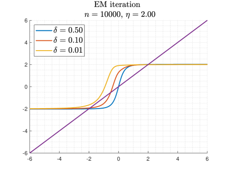
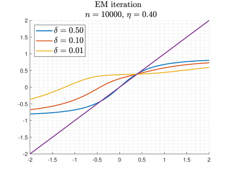
Figure 1: Illustration of $f(\theta,\delta\mid\eta,\delta)$ for $\eta=2$ and $\eta=0.4$.

We begin with the population iteration.

Theorem 4 (Population mean iteration, known weight, $d=1$).

The following holds:

1. The unique fixed point of $\theta\mapsto f(\theta\mid\eta,\delta)$ in $\mathbb{R}_{+}$ is $\theta=\eta$, and its fixed points in $\mathbb{R}_{-}$ are confined to the interval $(-\eta,0)$.

2. If $\theta_{0}\geqslant 0$ then the iteration $\theta_{t+1}=f(\theta_{t}\mid\eta,\delta)$ converges to $\eta$.

3. Let $\delta\leqslant\tilde{\delta}<1/2$ and $\theta_{0}\geqslant 0$. Consider the iteration $\tilde{\theta}_{t}=f(\tilde{\theta}_{t-1}\mid\eta,\tilde{\delta})$ such that $\theta_{0}=\tilde{\theta}_{0}\geqslant 0$. Then $|\eta-\tilde{\theta}_{t}|>|\eta-\theta_{t}|$ for all $t\geqslant 1$, i.e., the convergence is faster as $\delta$ is lower. The same holds for $\tilde{\delta}=1/2$ if $\theta_{0}>0$.

Though not crucial for the analysis or later derivations, we conjecture from exhaustive numerical evidence that there are only two spurious fixed points of $f(\theta)$ in $\mathbb{R}_{-}$, and furthermore, there exists $\delta_{\text{cr}}\in(0,1/2)$ such that the number of fixed points of $f(\theta)$ in $\mathbb{R}_{-}$ is

$$\begin{cases}2,&\delta\in(\delta_{\text{cr}},\frac{1}{2})\\ 1,&\delta=\delta_{\text{cr}}\\ 0,&\delta\in[0,\delta_{\text{cr}})\end{cases}\,.$$

Theorem 4 establishes global convergence properties for the unbalanced one-dimensional EM population iteration, when initializing either with the correct sign of the larger weight component, or with a neutral sign ($\theta=0$). Nonetheless, the illustration in Fig. 1 also demonstrates that initializing with the strictly wrong sign may lead to convergence to a spurious stable fixed point which is at a non-zero distance from $-\eta$, even when $n\to\infty$. Thus, a correct initialization of this iteration is both simple and crucial.

To describe the proof idea of Theorem 4, we briefly recall the properties of the balanced iteration $f(\theta\mid\eta,\frac{1}{2})$ and why this iteration globally converges. As evident from Fig. 1 (and proved in [38, Section 2]), $\theta\mapsto f(\theta\mid\eta,\frac{1}{2})$ is an odd increasing function which is concave on $\mathbb{R}_{+}$. It is not difficult to show (see also Proposition 23 in Appendix C) that in this case that the iteration must converge to one of the three unique fixed points $\theta=0,\pm\tilde{\theta}$. The general consistency property of EM then implies that $\tilde{\theta}=\eta$. Thus, for the balanced iteration, the concavity property provides a global property on the iteration which is used to establish global convergence.

The reduced uncertainty in the $\delta<1/2$ case hints that the iteration should converge faster and better than for the $\delta=1/2$ case. However, at the same time, the change from $\delta=1/2$ to $\delta<1/2$ breaks the symmetry in the iteration, and hence the concavity property of the iteration in $\mathbb{R}_{+}$. For example, the yellow iteration in Fig. 1 corresponding to $\delta=0.01$ shows that the iteration is non-concave around $\theta\approx 0.6$. Hence a different global property is required. The consistency property assures at $\theta=\eta$ the iteration is insensitive to $\delta$, and specifically that $f(\eta\mid\eta,\delta)=\eta$ for all $\delta$. As evident from Fig. 1, and as is true in general, for $\theta<\eta$ and $\theta>\eta$ a change in $\delta$ bares an opposite, yet consistent effect. The next proposition summarizes this property, along with another global property related to “oddness dominance” that will be used in the analysis of the empirical iteration.

Proposition 5.

Assume that $\eta>0$ and $\delta\in[0,\frac{1}{2}]$.

1. $f(\theta\mid\eta,\delta)\geqslant-f(-\theta\mid\eta,\delta)$ for all $\theta>0$.

2. $\delta\mapsto f(\theta\mid\eta,\delta)$ is non-increasing (resp. constant, resp. non-decreasing) for $\theta<\eta$ (resp. for $\eta=\theta$, resp. $\theta>\eta$).

The second property can be described as $\theta=\eta$ being a “pivot-point” for the iteration as $\delta$ is varied (see Fig. 1). Given the second property of Proposition 5, along with the known convergence for the case $\delta=1/2$, global convergence can be easily established for $\theta_{0}\geqslant 0$.

In order to prove property 2 in Proposition 5, one may assume an arbitrary and fixed true parameter $\eta>0$, and attempt to establish this property for all $\theta\in\mathbb{R}$. It turns out that if $\theta<0$, this property can be proved by a direct reasoning on $\frac{\partial}{\partial\delta}f(\theta\mid\eta,\delta)$. However, similar strategy seems daunting for $\theta>0$, and our proof is built on an indirect argument. More explicitly, for $\theta>0$ it is required to be proved that:

$$\frac{\partial f(\theta\mid\eta,\delta)}{\partial\delta}\;\;\begin{cases}>0,&0<\eta<\theta\\ =0,&\eta=\theta\\ <0,&\eta>\theta\end{cases}\,.$$ (16)

The proof of (16) is based on the following ideas:

• Analyzing $\frac{\partial}{\partial\delta}f(\theta\mid\eta,\delta)$ as a function of $\eta$, rather than as a function of $\theta$ directly. For this to be useful, we will need to analyze $\eta\in\mathbb{R}$ and not just $\eta\in\mathbb{R}_{+}$.

• Expressing $\frac{\partial}{\partial\delta}f(\theta\mid\eta,\delta)$ as a convolution of some function with a Gaussian kernel. We then exploit a variation diminishing property of Gaussian kernels which implies that if a function $h(\theta)$ has $k$ zero-crossings in $\mathbb{R}$, its convolution with a Gaussian kernel may only reduce the number of zero-crossings. See Proposition 25 in Appendix C.3 for a formal statement. This allows us to prove that $\eta\mapsto\frac{\partial}{\partial\delta}f(\theta\mid\eta,\delta)$ has a single crossing point for some $\theta_{0}$.

• Then, utilizing the consistency property, which states that $f(\theta\mid\eta,\delta)=\theta$ for $\theta=\eta$ and any $\delta$, establishes that $\theta_{0}=\theta$, and this results (16).

The idea of analyzing the iteration w.r.t. the true parameter $\eta$, rather than w.r.t. $\theta$ was previously used in [8], which utilized it in order to prove one-dimensional global convergence (as well as convergence rates) for the balanced iteration. While such an argument is not essential for this case (given the direct analysis in [38]), an idea in that spirit is useful here for proving a different global property.

We now turn to the empirical iteration. As we show next, the improved convergence in the unbalanced case compared to the balanced case stated in Theorem 4 compensates for the larger empirical error.

Theorem 6 (Empirical mean iteration, known weight, $d=1$).

Assume that $|\eta|\leqslant\mathsf{C}_{\theta}$, $|\rho_{*}|\leqslant\mathsf{C}_{\rho}$ and that the high probability event (15) holds. Consider the empirical mean EM iteration $\theta_{t}=f_{n}(\theta_{t-1})\equiv f_{n}(\theta_{t-1},\delta\mid\eta,\delta)$. There exists $n_{0}(\mathsf{C}_{\theta},\mathsf{C}_{\rho})$ and constants $\{\mathsf{C}_{i}^{(1)}(\mathsf{C}_{\theta},\mathsf{C}_{\rho})\}$ such that if $\rho_{*}>\mathsf{C}_{1}^{(1)}\sqrt{\omega_{1}}$ and $n\geqslant n_{0}$ then

$$\ell(\theta_{t},\eta)\leqslant\mathsf{C}_{2}^{(1)}\cdot\min\left\{\frac{\omega_{1}}{\rho},\frac{\omega_{1}}{\eta}\right\}$$

holds for all $t\geqslant\mathsf{T}_{\theta_{0}=0}^{(1)}$ where

$$\mathsf{T}_{\theta_{0}=0}^{(1)}:=\begin{cases}1,&\eta\leqslant\frac{\omega_{1}}{\rho}\\ \mathsf{C}_{3}^{(1)}\cdot\frac{1}{\rho^{2}}\log\left(\frac{\omega_{1}}{\mathsf{C}_{5}^{(1)}\rho}\right),&\frac{\omega_{1}}{\rho}\leqslant\eta\leqslant\mathsf{C}_{4}^{(1)}\rho\\ \mathsf{C}_{3}^{(1)}\cdot\left(\frac{1}{\rho\eta}+\frac{1}{\eta^{2}}\log\left(\frac{1}{\mathsf{C}_{6}^{(1)}\rho\omega_{1}}\right)\right),&\mathsf{C}_{4}^{(1)}\rho<\eta\leqslant\mathsf{C}_{\theta}\end{cases}$$

in case the iteration was initialized by $\theta_{0}=0$, and for all $t\geqslant\mathsf{T}_{\theta_{0}=\frac{1}{\rho}\mathbb{E}_{n}[X]}^{(1)}$ where

$$\mathsf{T}_{\theta_{0}=\frac{1}{\rho}\mathbb{E}_{n}[X]}^{(1)}:=\begin{cases}1,&\eta\leqslant\mathsf{C}_{4}^{(1)}\rho\\ \mathsf{C}_{3}^{(1)}\frac{1}{\eta^{2}}\log\left(\frac{1}{\mathsf{C}_{6}^{(1)}\rho\omega_{1}}\right),&\mathsf{C}_{4}^{(1)}\rho<\eta\leqslant\mathsf{C}_{\theta}\end{cases}$$

in case the iteration was initialized by $\theta_{0}=\frac{1}{\rho}\mathbb{E}_{n}[X]$ .

The proof uses the sandwiching method developed in [38] that bounds the empirical iteration $f_{-}(\theta)\leqslant f_{n}(\theta)\leqslant f_{+}(\theta)$ by the envelopes $f_{\pm}(\theta)=f(\theta)\pm\max\{|\theta|,\rho\}\cdot\omega_{1}$ (which holds with high probability), and the resulting iterations $\theta_{t}^{\pm}=f_{\pm}(\theta_{t-1})$ obtained when initializing those iterations and the empirical iteration with the same initial guess $\theta_{0}^{\pm}=\theta_{0}$. We consider both $\theta_{0}=0$ or $\theta_{0}=\frac{1}{\rho}\mathbb{E}_{n}[X]$. First, it is proved that all three iterations $\{\theta_{t}\},\{\theta_{t}^{\pm}\}$ converge to fixed points, $\eta_{n},\eta_{\pm}$ respectively. Then, the analysis is split into three regimes. For initialization at $\theta_{0}=0$:

1. If $\frac{\omega_{1}}{\rho}\lesssim\eta\lesssim\rho$ then the envelopes converge to fixed points $0<\eta_{-}\leqslant\eta_{n}\leqslant\eta_{+}$, and the envelopes are approximated as $f_{\pm}(\theta)\approx 1-c\rho^{2}$ for some $c>0$. Thus, the envelopes are contractions whose convergence times is on the order of $\tilde{O}(\frac{1}{\rho^{2}})$.

2. If $\rho\lesssim\eta$ then convergence has two phases. At the first phase, $\theta_{t}$ is low, and the iteration increases additively each step from $\theta_{0}=0$ by $\Omega(\rho^{2}\eta)$ at each iteration. Thus, after $T_{1}=O(\frac{1}{\rho\eta})$ iterations, $\theta_{t}=\Omega(\rho)$. At this point, the empirical error is $\omega_{1}\cdot\max\{\theta,\rho\}\lesssim\omega_{1}\theta$, to wit, the same empirical error as for the balanced iteration. Since the population iteration converges faster in the unbalanced case than in the balanced case (Theorem 4), and the empirical error in this case is of the same order, then the convergence of the unbalanced empirical iteration is only faster than that of the empirical balanced iteration. The latter was analyzed in [38, Theorem 3], and its result is utilized.

3. If $\eta\lesssim\frac{\omega_{1}}{\rho}$ then analysis similar to the previous cases shows that the upper envelope $\theta_{t}^{+}$ will increase, and will remain within the required statistical error, i.e., $0\leqslant\theta_{t}^{+}\lesssim\frac{\omega_{1}}{\rho}$, for all $t\geqslant 1$. On the other hand, for the lower envelope, it is not guaranteed that $f_{-}(0)>0$ , and so it is also not guaranteed that $\theta_{t}^{-}$ will increase and converge to a positive fixed point. If it does converge to a positive fixed point $\eta_{-}>0$, then $\eta_{-}<\eta_{+}$ must also hold, and, as for the upper envelope, $0\leqslant\theta_{t}^{-}\lesssim\frac{\omega_{1}}{\rho}$, for all $t\geqslant 1$. If, however, this is not the case and $f_{-}(0)<0$, then $\theta_{t}^{-}$ will decrease and converge to a negative fixed point $\eta_{-}<0$. In that event, the oddness domination property of the population iteration (Proposition 5, item 1) assures that $|\eta_{-}|\leqslant\eta_{+}$, and so the same statistical error $O(\frac{\omega_{1}}{\rho})$ is again assured.

For initialization at $\theta_{0}=\frac{1}{\rho}\mathbb{E}_{n}[X]$, the error in the first iteration is already within the statistical accuracy in Cases 1 and 3. For Case 2, it can be shown that the first phase of convergence does not occur, and the convergence is as in the balanced case.

2.3 The mean iteration for known weight at $d>1$

We now consider the general $d>1$ case. Recall that the $n$ i.i.d. samples are given by $X\sim(1-\delta)\cdot N(\theta_{*},I_{d})+\delta\cdot N(-\theta_{*},I_{d})$ where $\theta_{*}\in\mathbb{R}^{d}$ and $\delta\in(0,1/2)$ is known. For the population mean EM iteration we show that:

Theorem 7 (Population iteration, known weight, $d>1$).

Consider the population mean EM iteration $\theta_{t}=f(\theta_{t-1},\delta\mid\theta_{*},\delta)$. If $\langle\theta_{0},\theta_{*}\rangle\geqslant 0$ then $\lim_{t\to\infty}\theta_{t}=\theta_{*}$. Specifically, this holds for $\theta_{0}=0$.

As in the one-dimensional case, the idealized population iteration does not converge to a spurious fixed point, whenever the iteration is not initialized in a direction which has an obtuse angle with $\theta_{*}$ (which is the mean of the larger weight component, $1-\delta$). Furthermore, such initialization can be achieved by setting $\theta_{0}=0$, since $f(0,\delta\mid\theta_{*},\delta)=(1-2\delta)^{2}\cdot\theta_{*}$ which already points to the desired direction. Evidently, in this case, $\theta_{t}\propto\hat{\theta}_{*}$ for all $t\geqslant 1$. A slightly more general property holds for any initialization, and this is the basic ingredient of the proof which we describe next.

The proof of Theorem 7 is based on an observation made in [39, 8] that the population mean EM iteration is “trapped” to the two-dimensional space spanned by the true vector $\theta_{*}$ and the initial guess $\theta_{0}$. In [38] this observation was formulated in the following way. Let us denote $\eta:=\|\theta_{*}\|$ for brevity, let $V\sim(1-\delta)\cdot N(\eta,1)+\delta\cdot N(-\eta,1)$ and $W\sim N(0,1)$ be such that $V\perp\!\!\!\!\perp W$, and define:

$$F((a,b),\delta\mid\eta,\delta)=\mathbb{E}\left[V\tanh(aV+bW+\beta)\right]\,,$$

and

$$G((a,b),\delta\mid\eta,\delta)=\mathbb{E}\left[W\tanh(aV+bW+\beta)\right]\,,$$

where we omit the dependence in $(\eta,\delta)$ whenever it is inessential and simply write $F(a,b\mid\eta,\delta),\;G(a,b\mid\eta,\delta)$, or even just, $F(a,b),\;G(a,b)$. The following was proved in [38, Lemma 4] for the balanced case, but the proof is similar for any $\delta\in[0,1]$ and thus omitted.

Lemma 8 ([38, Lemma 4]).

Consider the population mean iteration $\theta_{t+1}=f(\theta_{t},\delta\mid\theta_{*},\delta)$, and define

$$\theta_{t}=a_{t}\cdot\hat{\theta}_{*}+b_{t}\cdot\xi_{t}$$

where $\eta=\|\theta_{*}\|$, $\hat{\theta}_{*}=\theta_{*}/\eta$, $\xi_{t}\perp\eta$ and $\|\xi_{t}\|=1$ such that $\operatorname{span}\{\theta_{*},\xi_{t}\}=\operatorname{span}\{\theta_{*},\theta_{t}\}$ and $b_{t}\geqslant 0$. Then, $\theta_{t}\in\operatorname{span}\{\theta_{0},\theta_{*}\}$ (i.e., $\xi_{t}=\xi_{0}$) for all $t$, and

$$a_{t+1} =F(a_{t},b_{t})$$

$$b_{t+1} =G(a_{t},b_{t})\,.$$

We refer to $F(\cdot)$ as the signal iteration and to $G(\cdot)$ as the orthogonal iteration. Lemma 8 thus implies that to analyze the iteration $\theta_{t+1}=f(\theta_{t},\delta\mid\theta_{*},\delta)$ it suffices to analyze the evolution of $\{a_{t},b_{t}\}$, and that $\theta_{t}\to\theta_{*}$ is equivalent to $a_{t}\to\eta$ and $b_{t}\to 0$.

In the balanced case, the population mean EM iteration was shown to globally converge to $\pm\theta_{*}$ by showing that the orthogonal error goes to zero unconditionally of the signal iteration, i.e., $b_{t}\to 0$ is always satisfied. Then, the problem is reduced to the one-dimensional iteration studied in the previous section. Essentially, this global property holds due to the fact that for $G(a,b\mid\eta,\frac{1}{2})$ is a concave increasing function with $G(a,0)=0$, and $\left.\frac{\partial}{\partial b}G(a,b)\right|_{b=0}<1$ [38, Lemma 5]. As in the one-dimensional case, in the unbalanced case, the lack of symmetry in case of $\delta<1/2$ breaks down the concavity property of $G(a,b\mid\eta,\delta)$, and so a different global property is required. This is achieved in the following proposition, which states properties of $G(a,b\mid\eta,\delta)$ w.r.t. the true parameters $(\eta,\delta)$, and specifically states that $G(a,b\mid\eta,\delta)$ is dominated by $G(a,b\mid\eta,1/2)$, and so the orthogonal iteration in case of $\delta<1/2$ converges faster than in the case of $\delta=1/2$.

Proposition 9.

1. Monotonicity w.r.t. $\delta$: If $a\geqslant 0$ then $\delta\mapsto G(a,b\mid\eta,\delta)$ is an increasing function on $[0,1/2]$.

2. Dominance w.r.t. $\delta$: Let $C_{f}>0$ be given. There exists $\mathsf{C}_{G,\rho}^{(d)}(\mathsf{C}_{\theta},\mathsf{C}_{\beta},C_{f})>0$ and $n_{0}(\mathsf{C}_{\theta},\mathsf{C}_{\beta},C_{f})$ such that for any $n\geqslant n_{0}$

   $$G(a,b\mid\eta,\delta)\leqslant G(a,b\mid\eta,\tfrac{1}{2})-\mathsf{C}_{G,\rho}^{(d)}\rho^{2}b\leqslant b\left(1-\frac{a^{2}+b^{2}}{2+4(a^{2}+b^{2})}-\mathsf{C}_{G,\rho}^{(d)}\rho^{2}\right)$$

   for all $(a,b,\eta)\in[0,C_{f}]^{2}\times[0,\mathsf{C}_{\theta}]$.

3. Monotonicity w.r.t. $\eta$: For $a\geqslant 0$, $\eta\mapsto G(a,b\mid\eta,\delta)$ is a decreasing function in $\eta\in[0,a+\frac{b^{2}}{a}]$.

4. Dominance w.r.t. $\eta$: Let $\mathsf{C}_{G,\eta}^{(d)}=3\mathsf{C}_{\theta}$. Then,

   $$G(a,b\mid\eta,\delta)\leqslant G(a,b\mid 0,\delta)+\mathsf{C}_{G,\eta}^{(d)}b\eta^{2}$$

   for all $(a,b,\eta)\in\mathbb{R}\times\mathbb{R}_{+}\times[0,\mathsf{C}_{\theta}]$.

Given items 1 and 2 of Proposition 9, it is evident that unconditional convergence of the orthogonal part of the iteration to zero is assured in the unbalanced case (and the convergence is only faster compared to the balanced case). After such convergence, the problem is almost precisely reduced to the one-dimensional setting in the signal iteration $\{a_{t}\}$, except for a small residual additive error resulting from orthogonal iteration. However, as was shown in the one-dimensional analysis, the unbalanced mean EM iteration may tolerate small additive term (therein, this was due to the term $\omega_{1}\rho$ which, unlike the error term $\omega_{1}\theta$ does not vanishes when $\|\theta\|\to 0$), and so this additive term does not prevent convergence.

We now turn to the empirical iteration:

Theorem 10 (Empirical iteration, known weight, $d>1$, large $\rho_{*}$).

Assume that $\|\theta_{*}\|\leqslant\mathsf{C}_{\theta}$ and that $|\rho_{*}|\leqslant\mathsf{C}_{\rho}$, and that the high probability event (15) holds. Consider the empirical mean EM iteration $\theta_{t}=f_{n}(\theta_{t-1},\delta\mid\theta_{*},\delta)$. There exists $n_{0}$ and constants $\{\mathsf{C}_{i}^{(d)}\}$ which depend on $(\mathsf{C}_{\theta},\mathsf{C}_{\rho})$ such that if $\rho_{*}>\mathsf{C}_{1}^{(d)}\sqrt{\omega}$ and $n\geqslant n_{0}$ then

$$\ell(\theta_{t},\theta_{*})\leqslant\mathsf{C}_{2}^{(d)}\min\left\{\frac{\omega}{\rho},\frac{\omega}{\eta}\right\}$$

holds for all $t\geqslant\mathsf{T}_{\theta_{0}}^{(d)}=\mathsf{T}_{\theta_{0}}^{(1)}+\mathsf{T}_{G}^{(d)}$ where either $\theta_{0}=0$ or $\theta_{0}=\frac{1}{\rho}\mathbb{E}_{n}[X]$, $\mathsf{T}_{\theta_{0}}^{(1)}$ is determined as in Theorem 6 by replacing $\omega_{1}\to\omega=\sqrt{\mathsf{C}_{\omega}\frac{d\log n}{n}}$ and where

$$\mathsf{T}_{G}^{(d)}:=\begin{cases}1,&\eta\leqslant\rho\\ \frac{C_{3}^{(d)}}{\eta^{2}}\cdot\log\left(C_{4}^{(d)}\frac{\omega}{\eta}\right),&\eta\geqslant\rho\end{cases}\,.$$

The proof of this theorem is based on splitting the analysis into three regimes $0<\eta\lesssim\frac{\omega}{\rho}$, $\frac{\omega}{\rho}\lesssim\eta\lesssim\rho$ and $\eta\gtrsim\rho$. First, it is shown that when initializing at either $\theta_{0}=0$ or $\theta_{0}=\frac{1}{\rho}\mathbb{E}_{n}[X]$, the orthogonal iteration satisfies $b_{t}=O(\frac{\omega}{\rho})$, and remains so for all iterations. In the $\eta\lesssim\frac{\omega}{\rho}$ regime, this is shown by the local behavior of $G(a,b\mid\eta,\delta)$ around $\eta\approx 0$ (Proposition 9, item 4). In the $\eta\gtrsim\frac{\omega}{\rho}$ this is proved by the dominance relation to the balanced orthogonal iteration (Proposition 9, items 1 and 2), along with a verification that $a_{t}$ remains positive for all iterations (so that these dominance relations are in fact valid). Given that $b_{t}=O(\frac{\omega}{\rho})$, the effect of the orthogonal iteration on the signal iteration is negligible, and it is essentially reduced to the one-dimensional iteration. The convergence time for this is $\mathsf{T}_{\theta_{0}}^{(1)}$ (when setting the specific initialization for $\theta_{0}$ ), and the resulting error for the signal iteration is $|a_{t}-\eta|=O(\min\{\frac{\omega}{\rho},\frac{\omega}{\eta}\})$. If $\eta<\rho$ then this is also the error rate for $\theta_{*}$ as $|\theta-\theta_{*}|=O(|a_{t}-\eta|+b_{t})$. If $\eta>\rho$, then the orthogonal iteration can be shown to decrease to $O(\frac{\omega}{\eta})$ after additional $\mathsf{T}_{G}^{(d)}$ iterations.

We next consider the case of $\rho_{*}$ which is too small to satisfy the condition of Theorem 10.

Proposition 11 (Empirical iteration, known weight, $d>1$, small $\rho_{*}$).

Assume that $\|\theta_{*}\|\leqslant\mathsf{C}_{\theta}$ and that the high probability event (15) holds. Further assume that the balanced EM weight iteration is run $\theta_{t}=f_{n}(\theta_{t-1},\delta=\frac{1}{2}\mid\theta_{*},\delta=\frac{1}{2})$ with random initialization as in Theorem 1. Let $\tilde{\theta}_{t}=s_{t}\theta_{t}$ where $s_{t}=\mathop{\mathrm{sign}}\langle\mathbb{E}_{n}[X],\theta_{t}\rangle$. Then, there exists $\mathsf{C}_{\rho}^{(d)}(\mathsf{C}_{\theta})>0$ such that if

$$\frac{\omega}{\eta}\leqslant\rho_{*}\leqslant\mathsf{C}_{1}^{(d)}\sqrt{\omega}\leqslant\mathsf{C}_{\eta}^{(d)}\eta\,,$$

then

$$\ell(\theta_{t},\theta_{*})\leqslant\mathsf{C}_{2}^{(d)}\frac{\omega}{\eta}$$

holds for all $t\geqslant\frac{\log n}{\|\theta_{*}\|^{2}}.$

Theorem 10 and Proposition 11 together imply Theorem 2, which is the main result of the paper.

2.4 The weight iteration for a fixed mean

In previous sections, we have considered the mean iteration assuming a known weight. In this section, we study the opposite extreme case, and study the weight iteration assuming a fixed mean $\theta$, and specifically, the case in which $\theta=\theta_{*}$ holds. In this case, the log-likelihood is given by

$$\rho_{\text{MLE}}=\operatorname*{arg\,max}_{\rho\in[0,1]}\sum_{i=1}^{n}\log\left(\frac{1+\rho}{2}e^{-\langle X_{i},\theta_{*}\rangle}+\frac{1-\rho}{2}e^{+\langle X_{i},\theta_{*}\rangle}\right).$$

As apparent and also well-known, the log-likelihood is a concave function of the unknown parameter $\rho$, and so, the EM algorithm is assured to converge to the MLE [35]. Alternatively, a simple method-of-moments estimator $\rho_{\text{MoM}}=\frac{1}{\|\theta\|}\langle\hat{\theta},\mathbb{E}_{n}[X]\rangle$ can be readily shown to achieve the minimax error rate for this problem, given roughly by $\min\{\frac{1}{\|\theta_{*}\|\sqrt{n}},1\}$ (see Theorem 22 in Appendix B). Nonetheless, in this section we directly analyze the EM iteration and provide statistical and computational guarantees similar to the previous sections. Despite the favorable behavior mentioned above, the analysis of the EM iteration is delicate, especially in the mismatched case $\theta\neq\theta_{*}$. Understanding the EM iteration in this setting may then further illuminate its basic features.

We thus assume in this section the model

$$P_{\rho}=\frac{1+\rho}{2}\cdot N(\theta_{*},1)+\frac{1-\rho}{2}\cdot N(-\theta_{*},1)$$

where $\delta=\frac{1-\rho}{2}$ . As in Section 2.3, the weight iteration can be written as

$$h(\rho,\theta\mid\theta_{*},\rho_{*}) =\mathbb{E}\left[\frac{(1+\rho)e^{\|\theta\|V}-(1-\rho)e^{-\|\theta\|V}}{(1+\rho)e^{\|\theta\|V}+(1-\rho)e^{-\|\theta\|V}}\right]$$

where $V\sim(\frac{1+\rho_{*}}{2})\cdot N(\langle\hat{\theta},\theta_{*}\rangle,1)+(\frac{1-\rho_{*}}{2})\cdot N(-\langle\hat{\theta},\theta_{*}\rangle,1)$ and $\hat{\theta}=\theta/\|\theta\|$. Similarly, the empirical iteration will be denoted by $h_{n}(\rho,\theta)$. In addition, since $|\rho_{*}|\leqslant\mathsf{C}_{\rho}$ is assumed, we may also consider truncated iterations given by $[h(\rho,\theta\mid\theta_{*},\rho_{*})]_{\mathsf{C}_{\rho}}$where

$$[t]_{\mathsf{C}_{\rho}}=\begin{cases}-\mathsf{C}_{\rho},&t<-\mathsf{C}_{\rho}\\ t,&-\mathsf{C}_{\rho}<t<\mathsf{C}_{\rho}\\ \mathsf{C}_{\rho},&t>\mathsf{C}_{\rho}\end{cases}\,.$$

Fig. 2 illustrates EM iteration (based on single runs of $n=10^{6}$ samples).

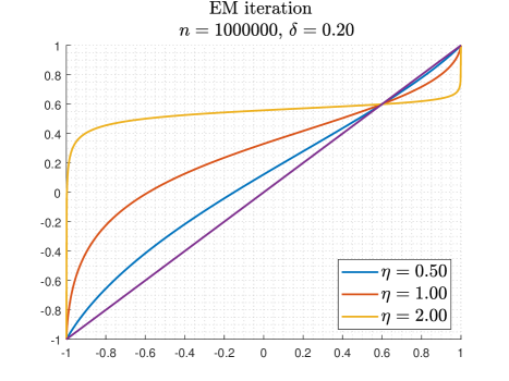
Figure 2: Illustration of $h(\rho,\eta\mid\eta,\rho_{*})$ for $\rho_{*}=0.6$ .

As expected, for a given fixed $\theta$, the iteration is essentially one-dimensional and does not depend on $d$. Note also that if $\langle\theta,\theta_{*}\rangle=0$ then $\rho_{*}$ is not identifiable, and, in accordance, the population iteration is useless; indeed $h(\rho)=\rho$ for this case. Regarding the population iteration, we have the following theorem:

Theorem 12 (Population weight iteration, fixed mean).

Assume that $\rho_{*}>0$ and that $\langle\theta,\theta_{*}\rangle\neq 0$. The following holds:

1. The iteration $h(\rho,\theta)$ has either two or three fixed points in $[-1,1]$. The boundaries $\rho=\pm 1$ are always fixed points. There exists a third fixed point $\rho_{\#}\in(-1,1)$ if and only if

   $$\left.\frac{\mathrm{d}}{\mathrm{d}\rho}h(\rho,\theta)\right|_{\rho=1}=e^{2\|\theta\|^{2}}\left[\left(\frac{1+\rho_{*}}{2}\right)e^{-2\langle\theta,\theta_{*}\rangle}+\left(\frac{1-\rho_{*}}{2}\right)\cdot e^{2\langle\theta,\theta_{*}\rangle}\right]>1$$ (17)

   and if it exists, it satisfies $\rho_{\#}\in(0,1)$ if $\langle\theta,\theta_{*}\rangle>0$ and $\rho_{\#}\in(-1,0)$ if $\langle\theta,\theta_{*}\rangle<0$. Specifically, condition (17) holds if $\|\theta\|>|\langle\hat{\theta},\theta_{*}\rangle|$, and, furthermore, if $\theta=\theta_{*}$ then $\rho_{\#}=\rho_{*}$.

2. If $\rho_{\#}>0$ exists then the iteration $\rho_{t+1}=h(\rho_{t},\theta)$ converges monotonically upwards (resp. downwards) to $\rho_{\#}$ if $\rho_{0}\in(-1,\rho_{\#}]$ (resp. $\rho_{0}\in[\rho_{\#},1)$).

The proof mainly utilizes the following properties of $\rho\mapsto h(\rho,\theta)$: It increases monotonically from $h(-1,\theta)=-1$ to $h(1,\theta)=1$, and in case there is a fixed point $\rho_{\#}\in(-1,1)$, its uniqueness follows from the fact that $h(\rho,\theta)$ changes its curvature only once as $\rho$ traverse from $-1$ to $1$ (from concave to convex).

A rough characterization of the influence of mismatched $\theta$ can be derived as follows. Note that for the method-of-moments estimator, a mismatch in the knowledge of $\theta_{*}$ when assuming the true vector is $\theta\neq\theta_{*}$ results in bias in estimation, such that, on the population level

$$\rho_{\text{MoM}}=\frac{1}{\|\theta\|}\langle\hat{\theta},\mathbb{E}[X]\rangle=\frac{1}{\|\theta\|}\langle\hat{\theta},\theta_{*}\rangle\cdot\rho_{*}\,.$$

Thus, $\rho_{\text{MoM}}<\rho_{*}$ if and only if $\langle\hat{\theta},\theta_{*}\rangle<\|\theta\|$. The next proposition shows the same effect for the EM iteration:

Proposition 13.

Assume that $\rho_{*}>0$ and that $\langle\hat{\theta},\theta_{*}\rangle>0$. Let $\rho_{\#}$ be the fixed point of $\rho\mapsto h(\rho,\theta)$ which satisfies $\rho_{\#}\in(-1,1)$ (if such exists). Then, $\rho_{\#}<\rho_{*}$ if and only if $\langle\hat{\theta},\theta_{*}\rangle<\|\theta\|$.

The proof of the global property in Proposition 13 is again based on the variation diminishing property of the Gaussian kernel, on consistency, and on exploring the location of the fixed point as a function of the true parameter $\theta_{*}$ for a fixed $\theta$.

The empirical weight iteration satisfies the following theorem:

Theorem 14 (Empirical weight iteration, known mean).

Assume that $\|\theta_{*}\|\leqslant\mathsf{C}_{\theta}$ and that $|\rho_{*}|\leqslant\mathsf{C}_{\rho}$, and that the high probability event (15) holds. Consider the truncated empirical weight iteration $\rho_{t}=[h_{n}(\rho_{t-1},\theta_{*}\mid\theta_{*},\rho_{*})]_{\mathsf{C}_{\rho}}$ when initialized with $\rho_{0}=0$. There exists $n_{0}(\mathsf{C}_{\theta},\mathsf{C}_{\rho})$ and constants $\{\mathsf{C}_{i}^{(\rho)}\}$ which depend on $(\mathsf{C}_{\theta},\mathsf{C}_{\rho})$ such that if $\|\theta_{*}\|>\mathsf{C}_{1}^{(\rho)}\frac{\omega_{1}}{\rho_{*}}$ and $n\geqslant n_{0}$ then

$$\ell(\rho_{t},\rho_{*})\leqslant\mathsf{C}_{2}^{(\rho)}\frac{\omega_{1}}{\|\theta_{*}\|}$$

holds for all $t\geqslant\mathsf{T}^{(\rho)}=\frac{\mathsf{C}_{3}^{(\rho)}}{\|\theta_{*}\|^{2}}$.

The proof is based on bounding the empirical iteration with envelopes of absolute error $\omega_{1}\|\theta_{*}\|$, and analyzing their convergence. As might be expected, both the error bound and convergence time diverge when $\|\theta_{*}\|\to 0$; In the extreme case $\|\theta_{*}\|=0$, $\rho_{*}$ is not identifiable at all. The error bound of the EM iteration (and thus, also the MLE) matches that of the method-of-moments estimator, and also the minimax error rate (Theorem 22 in Appendix B).

2.5 An open problem: joint mean and weight estimation

We have analyzed the EM algorithm for the model $P_{\theta,\delta}$ in case one of the parameters is known and the other is required to be estimated. We next briefly discuss the more challenging scenario in which both $\delta_{*}$ and $\theta_{*}$ are required to be jointly estimated. In this case, each of the parameters serves as a nuisance parameter for estimating the other one, and the exact statistical and computational rates of EM remains an open problem. We nonetheless briefly discuss several aspects of this problem.

For the idealized population version, it is straightforward to ensure convergence, even far from the solution by a proper “scheduling”, i.e., not necessarily running both (6)-(7) at each iteration. Specifically, a simple possible scheduling is “freezing” $\theta_{t}=\theta_{0}$ and running the weight iteration for $T_{0}$ steps until convergence, then freezing $\rho_{t}=\rho_{T_{0}}$ and running the mean iteration until convergence, and so on. The initialization and scheduling order will then affect convergence. If we set $\rho_{0}=0$ and run the balanced mean iteration $\theta_{t+1}=f(\theta_{t},\frac{1}{2}|\eta,\delta)$ it will converge to $\theta_{*}$. If we after this convergence we will run the weight iteration $\rho_{t+1}=h(\rho_{t},\theta_{*})$ it will converge to $\rho_{*}$. Thus, this scheduling globally converges to $(\theta_{*},\rho_{*})$. By contrast, while we have empirically observed that initializing with a frozen $\theta_{0}$ also globally converges, it is more challenging to establish via our methods. To see this, suppose for simplicity that $d=1$. Note that Proposition 13 hints the importance of assuring that $\theta_{0}>\theta_{*}\equiv\eta$ so that the weight iteration $\rho_{t+1}=h(\rho_{t},\theta_{0})$ will have a fixed point $\rho_{\#}<\rho_{*}$. If this condition does not hold, then the weight iteration might not have a fixed point $\rho_{\#}$ in $(-1,1)$, and the iteration will converge to the spurious fixed point of $\rho=1$. Thus, we would like to initialize with a frozen $\theta_{0}$ such that $|\theta_{0}|>\eta$. By our assumptions, this could be achieved, by setting $\|\theta_{0}\|=\mathsf{C}_{\theta}.$ Next, we freeze $\rho_{t}$ at the obtained fixed point $\rho_{\#}$, and run the mean iteration. The following property can be proved: Let $X\sim(1-\delta_{*})\cdot N(\eta,1)+\delta_{*}\cdot N(-\eta,1)$ with $\eta>0$ and assume that $\theta>0$. Then $f(\theta,\delta\mid\eta,\delta_{*})<f(\theta,\delta\mid\eta,\delta)$ if and only if $\delta_{*}>\delta$. Due to consistency and the convergence properties of $f(\theta,\delta\mid\eta,\delta)$ (Theorem 4), it can also be assured that $f(\theta,\delta\mid\eta,\delta_{*})$ has no fixed points in $(\eta,\infty)$, and has at least a single fixed point in $(0,\eta]$ (which might not be unique). Upon convergence to such a fixed point $\eta_{0}\leqslant\eta$, we may freeze it and run the weight iteration $h(\rho,\eta_{0})$. At this phase, since $\eta_{0}<\eta$ it is not clear that the weight iteration will have a non-trivial fixed point $\rho_{\#}\in(-1,1)$. A more delicate argument is required to assure global convergence for a scheduling that begins with a phase of frozen $\theta_{t}$. For the population iteration, we can always choose to begin with $\rho=0$ that is provably globally converges, but it is not clear if this scheduling is better in terms of the empirical iteration.

For the empirical iteration, the result of running the balanced mean EM iteration (or a spectral algorithm) can clearly be used to obtain with high probability an initial guess $\theta_{0}$ with $\|\theta_{0}-\theta_{*}\|=\tilde{O}(\sqrt{\omega})$ if $\|\theta_{*}\|\lesssim\sqrt{\omega}$ and $\|\theta_{0}-\theta_{*}\|=\tilde{O}(\frac{\omega}{\|\theta_{*}\|})$ otherwise. In the former case, $\theta_{0}$ is not informative regarding the direction of $\theta_{*}$, and so this initial guess is not expected to be better than $\theta_{0}=0$. When $\|\theta_{*}\|\gtrsim\sqrt{\omega}$, the initial guess has non-trivial angle with $\theta_{*}$, and so it seems beneficial to initialize with that $\theta_{0}$. Furthermore, the only possible case case in which EM algorithm can improve the error rate is $\rho_{*}>\|\theta_{*}\|\gtrsim\sqrt{\omega}.$ A possible direction to prove such a result, is to learn the stability of the mean iteration w.r.t. error in the weight and vice-versa. Specifically, using $\theta$ with $\|\theta-\theta_{*}\|\lesssim\frac{\omega}{\|\theta_{*}\|}$ in the iteration $\rho_{t+1}=h(\rho_{t},\theta\mid\theta_{*},\rho_{*})$ shifts the population fixed point by at most $O(\frac{\omega}{\|\theta_{*}\|^{2}})$, but this is larger than the shift due to the empirical error which is $O(\frac{\omega}{\|\theta_{*}\|})$. If, however, one can use $\rho$ with $|\rho-\rho_{*}|\lesssim\frac{\omega}{\|\theta_{*}\|}$ in the empirical mean iteration $\theta_{t+1}=f_{n}(\theta_{t},\rho_{t}\mid\theta_{*},\rho_{*})$ then this mismatch can be shown to be negligible compared to the empirical error. Thus, with this scheduling, the key point is how to finely estimate $\theta_{*}$ so that its effect on the weight iteration will be negligible. Nonetheless, if non trivial separation holds and $\theta_{*}=\Omega(1)$ then running the balanced EM mean iteration followed by the weight iteration leads to (nearly) optimal error rates.

3 Proofs for Section 2.2

3.1 Population iteration

The following lemma summarizes simple properties of the mean population iteration for $d=1$.

Lemma 15.

Assume that $\eta\geqslant 0$. The following properties hold for $f(\theta)\equiv f(\theta,\delta\mid\eta,\delta)$:

1. Iteration: $f(0)=(1-2\delta)^{2}\cdot\eta>0$, $f(\eta)=\eta$ (consistency) and $\lim_{\theta\to\infty}f(\theta)\leqslant\eta+1<\mathsf{C}_{\theta}+1$.

2. First order derivative: $f(\theta)$ is increasing on $\mathbb{R}$ and

   $$f^{\prime}(\theta)=\mathbb{E}\left[\frac{X^{2}}{\cosh^{2}(X\theta+\beta)}\right]=4\delta(1-\delta)\cdot\mathbb{E}\left[\frac{X^{2}}{\left((1-\delta)\cdot e^{X\theta}+\delta\cdot e^{-X\theta}\right)^{2}}\right]>0\,.$$

   At $\theta=0$

   $$f^{\prime}(0)=4\delta(1-\delta)\cdot\left[\eta^{2}+1\right]\,,$$

   and furthermore, if $\theta\geqslant\eta$ then

   $$f^{\prime}(\theta)\leqslant 2\sqrt{\delta(1-\delta)}e^{-\frac{1}{2}\eta^{2}}\leqslant 1-\frac{1}{4}\cdot\max\{\min\{\eta^{2},1\},\rho^{2}\}\,.$$

3. Second order derivative:

   $$f^{\prime\prime}(\theta)=-2\mathbb{E}_{X}\left[\frac{X^{3}\tanh(X\theta+\beta)}{\cosh^{2}(X\theta+\beta)}\right]=-8\cdot\delta(1-\delta)\cdot\mathbb{E}\left[X^{3}\frac{\left((1-\delta)\cdot e^{X\theta}-\delta\cdot e^{-X\theta}\right)}{\left((1-\delta)\cdot e^{X\theta}+\delta\cdot e^{-X\theta}\right)^{3}}\right]\,.$$

   Furthermore, there exists $\mathsf{C}^{\prime\prime}(\mathsf{C}_{\theta},\mathsf{C}_{\rho})$ such that for all $\theta\in\mathbb{R}$

   $$\left|f^{\prime\prime}(\theta)\right|\leqslant\mathsf{C}^{\prime\prime}\cdot\max\{\theta,\rho\}\,.$$

Proof.

We only explicitly prove non-trivial properties, or ones which are non-trivial extensions of [38, Lemma 3]. Let $Z\sim N(0,1)$.

1. The consistency property is well-known, but can also be proved explicitly:

   $$f(\eta) \overset{{\scriptstyle(a)}}{=}e^{-\eta^{2}/2}\cdot\mathbb{E}\left[Z\cdot\left((1-\delta)\cdot e^{Z\eta}-\delta\cdot e^{-Z\eta}\right)\right]$$

   $$=e^{-\eta^{2}/2}\cdot\mathbb{E}\left[Ze^{Z\eta}\right]-\delta e^{-\eta^{2}/2}\cdot\mathbb{E}\left[Z\cdot\left(e^{Z\eta}+e^{-Z\eta}\right)\right]$$

   $$\overset{{\scriptstyle(b)}}{=}e^{-\eta^{2}/2}\cdot\mathbb{E}\left[Ze^{Z\eta}\right]\overset{{\scriptstyle(c)}}{=}e^{-\eta^{2}/2}\cdot\mathbb{E}\left[\eta e^{Z\eta}\right]=\eta\,,$$

   where $(a)$ is by change of measure (see (51) in Appendix C.1), $(b)$ is by oddness of the argument in the second expectation, $(c)$ is by Stein’s identity (see (54) in Appendix C.1).

2. The bound on $f^{\prime}(\theta)$ for $\theta>\eta$ holds since

   $$f^{\prime}(\theta) \overset{{\scriptstyle(a)}}{=}e^{-\frac{1}{2}\eta^{2}}\cdot\mathbb{E}\left[Z^{2}\cdot\frac{4\delta(1-\delta)}{\left((1-\delta)\cdot e^{Z\theta}+\delta\cdot e^{-Z\theta}\right)^{2}}\cdot\left((1-\delta)\cdot e^{Z\eta}+\delta\cdot e^{-Z\eta}\right)\right]$$

   $$\overset{{\scriptstyle(b)}}{\leqslant}e^{-\frac{1}{2}\eta^{2}}\cdot\mathbb{E}\left[Z^{2}\cdot 2\sqrt{\delta(1-\delta)}\cdot\frac{(1-\delta)\cdot e^{Z\eta}+\delta\cdot e^{-Z\eta}}{(1-\delta)\cdot e^{Z\theta}+\delta\cdot e^{-Z\theta}}\right]$$

   $$\overset{{\scriptstyle(c)}}{=}2\sqrt{\delta(1-\delta)}e^{-\frac{1}{2}\eta^{2}}\cdot\mathbb{E}\left[\frac{1}{2}Z^{2}\cdot\frac{(1-\delta)\cdot e^{Z\eta}+\delta\cdot e^{-Z\eta}}{(1-\delta)\cdot e^{Z\theta}+\delta\cdot e^{-Z\theta}}+\frac{1}{2}Z^{2}\cdot\frac{(1-\delta)\cdot e^{-Z\eta}+\delta\cdot e^{Z\eta}}{(1-\delta)\cdot e^{-Z\theta}+\delta\cdot e^{Z\theta}}\right]$$

   $$\overset{{\scriptstyle(d)}}{\leqslant}e^{-\frac{1}{2}\eta^{2}}\cdot 2\sqrt{\delta(1-\delta)}\cdot\mathbb{E}\left[Z^{2}\right]$$ (18)

   where: $(a)$ is proved again by a change of measure; $(b)$ holds since by the inequality of arithmetic and geometric means, for any $a\geqslant 0$

   $$\frac{4\delta(1-\delta)}{(1-\delta)\cdot a+\delta\cdot a^{-1}}\leqslant 2\sqrt{\delta(1-\delta)}\,,$$

   $(c)$ follows since $Z\stackrel{{\scriptstyle d}}{{=}}-Z$; $(d)$ holds since

   $$\max_{\delta\in[0,\frac{1}{2}],\;a>b>1}\frac{1}{2}\cdot\frac{(1-\delta)\cdot b+\delta\cdot b^{-1}}{(1-\delta)\cdot a+\delta\cdot a^{-1}}+\frac{1}{2}\cdot\frac{(1-\delta)\cdot b^{-1}+\delta\cdot b}{(1-\delta)\cdot a^{-1}+\delta\cdot a}=1\,.$$ (19)

   To show that (19) holds, note that objective function on the l.h.s. is a convex function of $b$ for a given $(a,\delta)$, hence it is maximized for either $b=a$ or $b=1$. At $b=a$ the value of the objective is $1$. At $b=1$ we maximize over $a>1$:

   $$\max_{a>1}\frac{1}{2}\cdot\frac{1}{(1-\delta)\cdot a+\delta\cdot a^{-1}}+\frac{1}{2}\cdot\frac{1}{(1-\delta)\cdot a^{-1}+\delta\cdot a}$$

   $$=\max_{a>1}\frac{1}{2}\cdot\frac{a+a^{-1}}{(1-\delta)^{2}+\delta^{2}+\delta(1-\delta)\cdot\left(a+a^{-1}\right)}$$

   $$=\max_{c>2}\frac{1}{2}\cdot\frac{c}{(1-2\delta)^{2}+\delta(1-\delta)\cdot c}=1\,,$$

   where $c=a+a^{-1}$ was used, and the fact that the function to be maximized has a single maximum in $\mathbb{R}_{+}$ at $c=\frac{1-2\delta}{\sqrt{\delta}(1-\delta)}\leqslant 2$. Using $\delta=\frac{1-\rho}{2}$, we thus have $f^{\prime}(\theta)=\sqrt{1-\rho^{2}}\cdot e^{-\frac{1}{2}\eta^{2}}$. The final bound is obtained from $\sqrt{1-\rho^{2}}\leqslant 1-\frac{\rho^{2}}{2}$ and $e^{-\frac{1}{2}\eta^{2}}\leqslant\max\{e^{-1},1-\frac{\eta^{2}}{4}\}$.

3. The bound on the second derivative follows from $|\tanh(t)|\leqslant t$ and $\cosh(t)>1$.

∎

We next turn to prove Proposition 5. To this end, we need the following technical lemma:

Lemma 16.

Let $\beta>0$ be given, and let

$$s(u):=-\tanh(u+\beta)+\tanh(u-\beta)-\frac{1}{2\delta\cosh^{2}(u+\beta)}+\frac{1}{2(1-\delta)\cosh^{2}(u-\beta)}\,.$$ (20)

Then, $\frac{\mathrm{d}}{\mathrm{d}u}s(u)=0$ has a unique solution, this solution is negative, and $s(u)<0$ for all $u\in\mathbb{R}.$

Proof.

For $u<0$ the claim that $s(u)<0$ holds since both $\tanh(u-\beta)<\tanh(u+\beta)$ and $(1-\delta)\cosh^{2}(u-\beta)>\delta\cosh^{2}(u+\beta)$ hold when $\beta>0$. For $u\geqslant 0$, we begin by analyzing $\frac{\mathrm{d}}{\mathrm{d}u}s(u)$ and show that the real solution of $\frac{\mathrm{d}}{\mathrm{d}u}s(u)=0$ is negative and unique. Using the double-argument identities $1+\cosh(2t)=2\cosh^{2}(t)$, $\sinh(2t)=2\sinh(t)\cosh(t)$, the half-argument identity $\tanh(\frac{t}{2})=\frac{\sinh(t)}{\cosh(t)+1)}$ we obtain that the derivative is

$$\frac{\mathrm{d}s(u)}{\mathrm{d}u}=-\frac{1-\frac{1}{\delta}\tanh(u+\beta)}{\cosh^{2}(u+\beta)}+\frac{1-\frac{1}{1-\delta}\tanh(u-\beta)}{\cosh^{2}(u-\beta)}\,,$$ (21)

and thus get that $\frac{\mathrm{d}}{\mathrm{d}u}s(u)=0$ is equivalent to

$$\left[\frac{1+\cosh(2u-2\beta)}{1+\cosh(2u+2\beta)}\right]^{2}=\frac{1+\cosh(2u-2\beta)-\frac{1}{1-\delta}\sinh(2u-2\beta)}{1+\cosh(2u+2\beta)-\frac{1}{\delta}\sinh(2u+2\beta)}\,,$$

or, by using $\exp(2\beta)=\frac{1-\delta}{\delta}$ and denoting $\psi:=e^{2u}$, equivalent to

$$\frac{\left[2+\frac{1-\delta}{\delta}\psi^{-1}+\frac{\delta}{(1-\delta)}\psi\right]^{2}}{\left[2+\frac{\delta}{1-\delta}\psi^{-1}+\frac{1-\delta}{\delta}\psi\right]^{2}}=\frac{2+\frac{2-\delta}{\delta}\psi^{-1}-\frac{\delta^{2}}{(1-\delta)^{2}}\psi}{2+\frac{1+\delta}{1-\delta}\psi^{-1}-\frac{(1-\delta)^{2}}{\delta^{2}}\psi}\,.$$

After further algebraic manipulations, the last display can be shown to be equivalent to

$$(2\delta-1)\cdot\left[\delta\psi+1-\delta\right]\cdot\left[(1-\delta)\psi+\delta\right]\cdot\left[2\delta(1-\delta)\psi^{3}+3\delta(1-\delta)\psi^{2}+(1-2\delta)^{2}\psi-\delta(1-\delta)\right]=0.$$

As $\delta\in(0,\frac{1}{2})$ and $\psi>0$, the only real solution to this equation is the solution to

$$2\delta(1-\delta)\psi^{3}+3\delta(1-\delta)\psi^{2}+(1-2\delta)^{2}\psi-\delta(1-\delta)=0.$$

The l.h.s. of the last display is an increasing function of $\psi\in\mathbb{R}_{+}$ with value $-\delta(1-\delta)$ at $\psi=0$ and a strictly positive value at $\psi=1$. Thus, the above equation has a single real solution which belongs to $(0,1)$. Hence, $\frac{\mathrm{d}}{\mathrm{d}u}s(u)=0$ has a unique solution, and this solution is negative.

We next use this property $\frac{\mathrm{d}}{\mathrm{d}u}s(u)$ to show that $s(u)<0$ for all $u\geqslant 0$. As $s(0)=4(2\delta-1)<0$ and $\lim_{u\to\infty}s(u)=0$, the mean value theorem implies that $\frac{\mathrm{d}}{\mathrm{d}u}s(u)$ must be strictly positive for some $u>0$. Since $\frac{\mathrm{d}}{\mathrm{d}u}s(u)\neq 0$ for $u>0$, $s(u)$ must be increasing for all $u>0$. Since $\lim_{u\to\infty}s(u)=0$ holds, $s(u)\geqslant 0$ is impossible for $u>0$. ∎

Proof of Proposition 5.

Let $U\sim N(\eta,1)$. To prove the first property, we write

$$f(\theta\mid\eta,\delta)+f(-\theta\mid\eta,\delta)$$

$$=\mathbb{E}\left[X\cdot\tanh(X\theta+\beta)-X\cdot\tanh(X\theta-\beta)\right]$$

$$=(1-2\delta)\cdot\mathbb{E}\left[U\cdot\tanh(U\theta+\beta)-U\cdot\tanh(U\theta-\beta)\right]$$

$$\geqslant 0$$

which holds since $u\mapsto u\cdot\tanh(u\theta+\beta)-u\cdot\tanh(u\theta-\beta)$ is an odd function, that is positive on $\mathbb{R}_{+}$.

To prove the second property, we write the iteration as

$$f(\theta\mid\eta,\delta)=\mathbb{E}\left[(1-\delta)\cdot U\tanh(U\theta+\beta)+\delta\cdot U\tanh(U\theta-\beta)\right],$$

and then analyze its derivative w.r.t. $\delta$

$$\frac{\partial f(\theta\mid\eta,\delta)}{\partial\delta} =\mathbb{E}\left[-U\tanh(U\theta+\beta)+U\tanh(U\theta-\beta)\right]$$

$$\hphantom{=}-\frac{1}{2\delta(1-\delta)}\mathbb{E}\left[\frac{(1-\delta)U}{\cosh^{2}(U\theta+\beta)}-\frac{\delta U}{\cosh^{2}(U\theta-\beta)}\right]\,.$$

To prove the required property, we will show that

$$\frac{\partial f(\theta\mid\eta,\delta)}{\partial\delta}\;\;\begin{cases}<0,&\theta<\eta\\ =0,&\eta=\theta\\ >0,&\theta>\eta\end{cases}$$

and to this end we split the analysis to the cases $\theta=0$, $\theta<0$ and $\theta\geqslant 0$.

Case $\theta=0$

In this case, trivially, $\left.\frac{\partial f(\theta\mid\eta,\delta)}{\partial\delta}\right|{}_{\theta=0}=-4(1-2\delta)\eta<0$ for $\eta>0$ and $\delta\in(0,\frac{1}{2})$.

Case $\theta<0$

Let

$$q_{1}(u):=-u\tanh(u\theta+\beta)+u\tanh(u\theta-\beta)$$

and note that since $\tanh$ is monotonically increasing and negative for $t<0$, it holds that $q_{1}(u)$ is an odd function, and $q_{1}(u)<0$ for all $u>0$. Thus $\mathbb{E}[q_{1}(U)]<0$. Also let

$$q_{2}(u):=\frac{(1-\delta)u}{\cosh^{2}(u\theta+\beta)}-\frac{\delta u}{\cosh^{2}(u\theta-\beta)}\,.$$

Since $\cosh$ is an even function with a unique minimum at $t=0$, it holds that

$$q_{2}(u)=u\left[\frac{(1-\delta)}{\cosh^{2}(u\theta+\beta)}-\frac{\delta}{\cosh^{2}(u\theta-\beta)}\right]>0\,,$$

and

$$q_{2}(u)+q_{2}(-u) =\frac{(1-\delta)u}{\cosh^{2}(u\theta+\beta)}-\frac{\delta u}{\cosh^{2}(u\theta-\beta)}-\frac{(1-\delta)u}{\cosh^{2}(u\theta-\beta)}+\frac{\delta u}{\cosh^{2}(u\theta+\beta)}$$

$$=u\left(\frac{1}{\cosh^{2}(u\theta+\beta)}-\frac{1}{\cosh^{2}(u\theta-\beta)}\right)>0$$

for any $u>0$. Thus $q_{2}(u)>-q_{2}(-u)$ for $u>0$, and $\mathbb{E}[q_{2}(U)]>0$ (see Appendix C.1). The required property then follows since $\frac{\partial f(\theta\mid\eta,\delta)}{\partial\delta}=\mathbb{E}\left[q_{1}(U)\right]-\frac{1}{2\delta(1-\delta)}\mathbb{E}\left[q_{2}(U)\right]<0$.

Case $\theta>0$

We follow the ideas outlined in the discussion following the statement of the proposition. We note that $\frac{\partial f(\theta\mid\eta,\delta)}{\partial\delta}=\mathbb{E}\left[U\cdot s(U)\right]$ where $s(u)$ is as defined in (20), and so

$$\frac{\partial f(\theta\mid\eta,\delta)}{\partial\delta}=\left[\eta\cdot s(\theta\eta)\right]*\varphi(\eta)$$ (22)

where $\varphi(\eta):=\frac{1}{\sqrt{2\pi}}\cdot e^{-\eta^{2}/2}$ is the Gaussian kernel, and the convolution is w.r.t. $\eta$.

We begin by proving that $\eta\mapsto\frac{\partial f(\theta\mid\eta,\delta)}{\partial\delta}$ has at least a single zero-crossing in $\mathbb{R}_{+}$ by showing that for $\eta=0$ and as $\eta\to\infty$:

$$\left.\frac{\partial f(\theta\mid\eta,\delta)}{\partial\delta}\right|_{\eta=0}>0,\;\;\frac{\partial f(\theta\mid\eta,\delta)}{\partial\delta}\uparrow 0\text{ as }\eta\to\infty.$$

At $\eta=0$, using the definitions of $q_{1}(u)$ and $q_{2}(u)$, and recalling that $Z\sim N(0,1)$

$$\left.\frac{\partial f(\theta\mid\eta,\delta)}{\partial\delta}\right|_{\eta=0} =\mathbb{E}\left[q_{1}(Z)\right]-\frac{1}{2\delta(1-\delta)}\mathbb{E}\left[q_{2}(Z)\right]$$

$$\overset{{\scriptstyle(a)}}{=}-\frac{1}{2\delta(1-\delta)}\mathbb{E}\left[q_{2}(Z)\right]$$

$$=-\frac{1}{2\delta(1-\delta)}\mathbb{E}\left[q_{2}(Z)+q_{2}(-Z)\right]$$

$$=-\frac{1}{2\delta(1-\delta)}\mathbb{E}\left[Z\left(\frac{1}{\cosh^{2}(Z\theta+\beta)}-\frac{1}{\cosh^{2}(Z\theta-\beta)}\right)\right]$$

$$\overset{{\scriptstyle(b)}}{>}0$$

where $(a)$ is since $q_{1}(u)$ is an odd function, and $(b)$ is since for $\theta>0$ and any $u\in\mathbb{R}$

$$u\left(\frac{1}{\cosh^{2}(u\theta+\beta)}-\frac{1}{\cosh^{2}(u\theta-\beta)}\right)<0\,.$$

For $\eta\to\infty$, we note that the first term in the limit of $\frac{\partial f(\theta\mid\eta,\delta)}{\partial\delta}$ is

$$\lim_{\eta\to\infty}\mathbb{E}\left[-(Z+\eta)\tanh\left((Z+\eta)\theta+\beta\right)+(Z+\eta)\tanh\left((Z+\eta)\theta-\beta\right)\right]$$

$$=\mathbb{E}\left[\lim_{\eta\to\infty}\left(-(Z+\eta)\left[\tanh\left((Z+\eta)\theta+\beta\right)-\tanh\left((Z+\eta)\theta-\beta)\right)\right]\right)\right]$$

by dominated convergence theorem. Then, by L’Hôpital

$$\lim_{\eta\to\infty}(z+\eta)\left[\tanh\left((z+\eta)\theta+\beta\right)-\tanh\left((z+\eta)\theta-\beta\right)\right]$$

$$=\lim_{\eta\to\infty}\frac{\left[\tanh\left((z+\eta)\theta+\beta\right)-\tanh\left((z+\eta)\theta-\beta\right)\right]}{(z+\eta)^{-1}}$$

$$=\lim_{\eta\to\infty}\theta\frac{\left[\frac{1}{\cosh^{2}\left((z+\eta)\theta+\beta\right)}-\frac{1}{\cosh^{2}\left((z+\eta)\theta-\beta\right)}\right]}{-(z+\eta)^{-2}}=0$$

since $\cosh(t)>e^{t}/2$ for $t>0$. The second term in the limit of $\frac{\partial f(\theta\mid\eta,\delta)}{\partial\delta}$ can be analyzed similarly and also equals zero. The fact that the limit of $\frac{\partial f(\theta\mid\eta,\delta)}{\partial\delta}$ to $0$ is from below, can be deduced from $\eta\cdot s(\theta\eta)<0$ for all $\eta>0$ (Lemma 16) and the convolution relation (22).

Next, we prove that the zero-crossing of $\eta\mapsto\frac{\partial f(\theta\mid\eta,\delta)}{\partial\delta}$ in $\mathbb{R}_{+}$ is unique. The function $\eta\mapsto\eta\cdot s(\theta\eta)$ has a unique zero-crossing at $\eta=0$ since Lemma 16 implies that $s(\theta\eta)<0$ for all $\eta>0$ . Furthermore, for any given $\theta$, $\eta\mapsto\eta\cdot s(\theta\eta)$ is a bounded function. Indeed, $\eta\cdot s(\theta\eta)$ is clearly bounded for $|\eta|\leqslant 1$. For $|\eta|>1$, note that using $\tanh(t)=1-\frac{e^{-t}}{\cosh(t)}$, it holds that for any $\eta>0$

$$\left|\tanh(\theta\eta+\beta)-\tanh(\theta\eta-\beta)\right|$$

$$=e^{-\theta\eta}\left|\frac{e^{-\beta}}{\cosh(\theta\eta+\beta)}-\frac{e^{\beta}}{\cosh(\theta\eta-\beta)}\right|$$

$$\leqslant e^{-\theta\eta}\cdot 2e^{\beta},$$

and analogous result holds for $\eta<0$. Also, using $\cosh(t)\geqslant 1+\frac{t^{2}}{2}$, it holds that

$$\left|\left(\frac{1}{2\delta\cosh^{2}(\theta\eta+\beta)}-\frac{1}{2(1-\delta)\cosh^{2}(\theta\eta-\beta)}\right)\right|\leqslant\frac{1}{2\delta\left(1+\frac{\theta\eta+\beta}{2}\right)^{2}}+\frac{1}{2(1-\delta)\left(1+\frac{\theta\eta-\beta}{2}\right)^{2}}\,.$$

Hence, $\left|\eta\cdot s(\theta\eta)\right|\leqslant|\eta|\cdot[e^{-\theta|\eta|}\cdot 2e^{\beta}+\frac{1}{\delta\theta^{2}\eta^{2}}]$ which is bounded for all $|\eta|>1$.

The variation diminishing property of the Gaussian kernel (Proposition 25, Appendix C.3), and the convolution relation (22) imply that $\frac{\partial f(\theta\mid\eta,\delta)}{\partial\delta}$ has at most a single zero-crossing as a function of $\eta$. From all the above, $\frac{\partial f(\theta\mid\eta,\delta)}{\partial\delta}$ has exactly a single zero-crossing for some $\eta>0$. The consistency property implies that $\left.\frac{\partial f(\theta\mid\eta,\delta)}{\partial\delta}\right|_{\theta=\eta}=0$, and so this zero-crossing must occur at $\eta=\theta$. From this, (16) follows. ∎

Proof of theorem 4.

Recall that $\pm\eta$ and $0$ are the only fixed points of the balanced iteration $f(\theta,\frac{1}{2}\mid\eta,\frac{1}{2})$, and that $f(|\theta|,\frac{1}{2}\mid\eta,\frac{1}{2})>|\theta|$ for $0<|\theta|<\eta$, and $f(|\theta|,\frac{1}{2}\mid\eta,\frac{1}{2})<|\theta|$ for $|\theta|>\eta$. The claim then follows from Proposition 5, item 2. The last two claims follow from Proposition 23, items 4 and 5. ∎

3.2 Empirical iteration

Proof of Theorem 6.

We analyze the empirical iteration $f_{n}(\theta)\equiv f_{n}(\theta,\delta\mid\eta,\delta)$. From Lemma 15 and assuming the high probability event (15), it holds that

$$|f_{n}(\theta)|\leqslant\mathsf{C}_{\theta}+1+\omega\leqslant\mathsf{C}_{\theta}+2$$

for all $n$ sufficiently large, and that

$$f_{n}(\theta)\geqslant f_{-}(\theta):=f(\theta)-\max\{|\theta|,\rho\}\cdot\omega\,,$$ (23)

and

$$f_{n}(\theta)\leqslant f_{+}(\theta):=f(\theta)+\max\{|\theta|,\rho\}\cdot\omega\,,$$ (24)

where we abbreviate here $\omega\equiv\omega_{1}=\sqrt{\mathsf{C}_{\omega}\frac{\log n}{n}}$ and $f_{\pm}(\theta)$ will be referred to as the lower ($-$) and upper ($+$) envelopes. We consider the empirical iteration $\theta_{t+1}=f_{n}(\theta_{t})$ as well as the lower and upper envelopes iterations $\theta_{t+1}^{\pm}=f_{\pm}(\theta_{t}^{\pm})$, all which are initialized at the same point, to wit, $\theta_{0}=\theta_{0}^{\pm}$. We begin by thoroughly analyzing the initialization $\theta_{0}=0$ and then briefly discuss the initialization $\theta_{0}=\frac{1}{\rho}\mathbb{E}_{n}[X]$ (which is similar and simpler). In the first step of the proof, we show that $\{\theta_{t}\}$ and $\{\theta_{t}^{\pm}\}$ all converge monotonically to fixed points. In the second step, we analyze the convergence time and the distance between the fixed points. We split the analysis into three different regimes for $\eta$.

Fixed points

We show that $\{\theta_{t}\}$ and $\{\theta_{t}^{\pm}\}$ converge monotonically to fixed points, which we denote, respectively, by $\eta_{n}$ and $\eta_{\pm}$. We use several intuitive properties of convergence of one-dimensional iterations, which are formally stated and proved in Proposition 23, items 1 and 4.

For the empirical iteration $f_{n}(\theta)$, since

$$f^{\prime}_{n}(\theta)=\mathbb{E}_{n}\left[\frac{X^{2}}{\cosh^{2}(X\theta+\beta)}\right]>0$$

and $f_{n}(\theta)$ is bounded by assumption, $\{\theta_{t}\}$ converges monotonically to a fixed point $\eta_{n}$, and is either increasing or decreasing according to the sign of $f_{n}(0)$.

For the upper envelope $f_{+}(\theta)$, recall from Lemma 15 that $f(\theta)$ is increasing and bounded. So $\lim_{\theta\to\infty}f^{\prime}(\theta)=0$. Hence, $f_{+}(\theta)$ is increasing, and for $n>n_{0}(\mathsf{C}_{\omega})$ it holds that $\lim_{\theta\to\infty}f^{\prime}_{+}(\theta)<1$. Thus $\{\theta_{t}^{+}\}$ is increasing and converges to a fixed point $\eta_{+}$.

For the lower envelope $f_{-}(\theta)$, first note that there exists $n_{1}(\mathsf{C}_{\theta},\mathsf{C}_{\rho})$ such that $f_{-}(\theta)$ is increasing for all $\theta\in[-\mathsf{C}_{\theta},\mathsf{C}_{\theta}]$ since

$$f_{-}^{\prime}(\theta)\geqslant f^{\prime}(\theta)-\omega\geqslant\min_{0\leqslant\eta\leqslant\mathsf{C}_{\theta}}\mathbb{E}\left[\frac{X^{2}}{\cosh^{2}(|X|\mathsf{C}_{\theta}+\beta)}\right]-\omega>0\,.$$ (25)

If $f_{-}(0)>0$ then since $f(\theta)$ has a unique fixed point $\eta$ in $[0,\infty)$, $f_{-}(\theta)$ must have a fixed point in $[0,\eta]$, and no fixed points in $[\eta,\infty)$, and $\{\theta_{t}^{-}\}$ is increasing to one of the fixed points in $[0,\eta)$. If $f_{-}(0)<0$ then as the negative fixed points of $f(\theta)$ are confined to $[-\eta,0]$ (Theorem 4) similar reasoning as for the upper envelope leads to the conclusion that $\{\theta_{t}^{-}\}$ is decreasing and converges to some fixed point $\eta_{-}<0$. Furthermore, since the negative fixed points of $f(\theta)$ are confined to $[-\eta,0]$ (Theorem 4) and since $f(\theta)\geqslant-f(-\theta)$ for all $\theta>0$ (Proposition 5, item 1) the minimal negative fixed point $\underline{\eta}_{-}<0$ satisfies $|\underline{\eta}_{-}|\leqslant|\eta_{+}|$.

Stochastic error and convergence time

We now prove bounds on the stochastic error and on the required number of iterations for convergence. We will use constants $C_{1},C_{2},C_{3}>0$ which satisfy relations that will be specified throughout the proof. Assume that $\rho\geqslant C_{1}\sqrt{\omega}$. We split the analysis to three regimes for $\eta$ given by $[0,\frac{\omega}{\rho}]$, $[\frac{\omega}{\rho},C_{2}\rho]$ and $[C_{2}\rho,\mathsf{C}_{\theta}]$ where $C_{1}\geqslant\sqrt{1/C_{2}}$ is assumed so that these are three non-empty intervals. For simplicity, we assume that $C_{2}\leqslant 1$ (its value will eventually be chosen to be sufficiently small).

Case 1 - $\eta\in[\frac{\omega}{\rho},C_{2}\rho]$: For $\theta\geqslant\eta$, Lemma 15 implies that

$$f^{\prime}_{+}(\theta)\leqslant 1-\frac{\rho^{2}}{4}+\omega\,.$$

Thus, assuming $C_{1}\geqslant\sqrt{12}$ then $f^{\prime}_{+}(\theta)\leqslant 1-\frac{\rho^{2}}{6}.$ For $0\leqslant\theta<\eta$, we have

$$\left|f^{\prime\prime}(\theta)\right|\leqslant\mathsf{C}^{\prime\prime}\cdot\max\{\eta,\rho\}\leqslant\mathsf{C}^{\prime\prime}\rho\,,$$

and using $f^{\prime}_{+}(\theta)=f^{\prime}_{+}(\eta)-\int_{\theta}^{\eta}f^{\prime\prime}(\tilde{\theta})\mathrm{d}\tilde{\theta}$, it holds that

$$f^{\prime}_{+}(\theta) \leqslant 1-\frac{\rho^{2}}{4}+\mathsf{C}^{\prime\prime}\rho(\eta-\theta)+\omega$$

$$\leqslant 1-\frac{\rho^{2}}{4}+\mathsf{C}^{\prime\prime}\eta\rho+\omega$$

$$\leqslant 1-\frac{\rho^{2}}{4}+\mathsf{C}^{\prime\prime}C_{2}\rho^{2}+\omega\,.$$

Assuming that $C_{1}\geqslant\sqrt{12}$ and $C_{2}\leqslant\frac{1}{12\cdot\mathsf{C}^{\prime\prime}}$ we get that $f^{\prime}_{+}(\theta)\leqslant 1-\frac{\rho^{2}}{12}$. Thus, $f_{+}(\theta)$ is a contraction for $\theta\in[0,\infty)$. Hence, so is $f_{-}(\theta)$ (as $0\leqslant f^{\prime}_{-}(\theta)\leqslant f^{\prime}_{+}(\theta)$). Furthermore, it holds that $f_{+}(0)>f_{-}(0)=f(0)-\rho\omega>0$ for all $n\geqslant n_{2}(\mathsf{C}_{\theta},\mathsf{C}_{\rho})$. Thus both $\theta_{t}^{\pm}$ are increasing and converge to fixed points $\eta_{\pm}>0$ where $\eta_{+}\geqslant\eta\geqslant\eta_{-}$ and satisfy $\eta_{\pm}-\theta_{t}^{\pm}\leqslant\eta_{\pm}(1-\frac{\rho^{2}}{12})^{t}$ (Proposition 23, item 6). We next analyze the errors $\epsilon_{-}=\eta-\eta_{-}>0$ and $\epsilon_{+}=\eta_{+}-\eta>0$. For the error of the lower envelope, let $\theta\in[\eta_{-},\eta]$ and recall that $\eta_{-}\leqslant\eta\leqslant C_{2}\rho$. Then, $f^{\prime\prime}(\theta)\geqslant-\mathsf{C}^{\prime\prime}\rho$ and so

$$f^{\prime}(\eta)\geqslant f^{\prime}(\theta)-\mathsf{C}^{\prime\prime}\rho(\eta-\theta)\,,$$

as well as $f_{-}(\theta)>f(\theta)-\rho\omega.$ Hence

$$\eta-\rho\omega =f_{-}(\eta)$$

$$=f_{-}(\eta_{-})+\int_{\eta_{-}}^{\eta}f_{-}^{\prime}(\theta)\cdot\mathrm{d}\theta$$

$$\leqslant\eta_{-}+\int_{\eta_{-}}^{\eta}f^{\prime}(\theta)\cdot\mathrm{d}\theta$$

$$\leqslant\eta_{-}+f^{\prime}(\eta)\epsilon_{-}+\mathsf{C}^{\prime\prime}\rho\left(\eta\epsilon_{-}-\frac{\eta^{2}-\eta_{-}^{2}}{2}\right)$$

$$\leqslant\eta_{-}+f^{\prime}(\eta)\epsilon_{-}+\mathsf{C}^{\prime\prime}C_{2}\rho^{2}\epsilon_{-}\,.$$

The above implies $\epsilon_{-}(1-f^{\prime}(\eta)-C_{2}\rho^{2})\leqslant\rho\omega$ and since $f^{\prime}(\eta)\leqslant 1-\frac{\rho^{2}}{4}$ then if $C_{2}\leqslant\frac{1}{8}$ we obtain $\eta-\eta_{-}\leqslant 8\frac{\omega}{\rho}$. Since $\eta_{-}-\theta_{t}^{-}\leqslant\eta_{-}(1-\frac{\rho^{2}}{12})^{t}\leqslant\mathsf{C}_{\theta}(1-\frac{\rho^{2}}{12})^{t}$ it holds that $\eta_{-}-\theta_{t}^{-}\leqslant 8\frac{\omega}{\rho}$ for all $t\geqslant\frac{12}{\rho^{2}}\log\left(\frac{\mathsf{C}_{\theta}}{8}\cdot\frac{\rho}{\omega}\right)$ (Proposition 23, item 6) and so also $\eta-\theta_{t}^{-}\leqslant 16\frac{\omega}{\rho}$. The analysis for $\eta_{+}$ is similar:

$$\eta_{+} =f_{+}(\eta_{+})$$

$$=f_{+}(\eta)+\int_{\eta}^{\eta_{+}}f_{+}^{\prime}(\theta)\cdot\mathrm{d}\theta$$

$$=\eta+\rho\omega+\epsilon_{+}\left(f^{\prime}(\eta)+\omega\right)\,.$$

Then, since $\eta\leqslant C_{2}\rho$ and $f^{\prime}(\theta)\leqslant 1-\frac{\rho^{2}}{4}$ it holds that $\epsilon_{+}(\frac{\rho^{2}}{4}-\omega)\leqslant\rho\omega$ for all $\theta>\eta$. Since $\rho\geqslant C_{1}\sqrt{\omega}$, assuming $C_{1}\geqslant\sqrt{8}$ we get $\eta_{+}-\eta\leqslant 8\frac{\omega}{\rho}$. Furthermore, for all $n\geqslant n_{3}(\mathsf{C}_{\omega})$, $\eta_{+}\leqslant 2\eta$ and so for all $t\geqslant\frac{12}{\rho^{2}}\log\left(\frac{\mathsf{C}_{\theta}}{4}\frac{\rho}{\omega}\right)$ it holds that $|\eta-\theta_{t}^{+}|\leqslant 16\frac{\omega}{\rho}$.

Case 2 - $\eta\in[C_{2}\rho,\mathsf{C}_{\theta}]$: The convergence has two phases. The time spent in phase $1$ (resp. phase $2$) until the required convergence is assured will be denoted by $T_{1}$ (resp. $T_{2}$).

1. We show that there exists $C_{3}\leqslant\frac{1}{2}$ sufficiently small and $C_{1}$ sufficiently large such that $f_{-}(\theta)>\theta+\frac{1}{6}\rho^{2}\eta$ holds for all $\theta\in[0,C_{3}\rho]$ (note that $\rho>2\theta$ is assured). In turn, this inequality is satisfied if

   $$f(\theta)>\theta+\omega(\theta+\rho)+\frac{1}{6}\rho^{2}\eta$$ (26)

   holds. Since

   $$f^{\prime}(\theta) =f^{\prime}(0)+\int_{0}^{\theta}f^{\prime\prime}(\tilde{\theta})\cdot\mathrm{d}\tilde{\theta}$$

   $$\geqslant(1-\rho^{2})(1+\eta^{2})-\frac{\mathsf{C}^{\prime\prime}}{2}\theta^{2}-\mathsf{C}^{\prime\prime}\rho\theta\,,$$

   and as $f(0)=\rho^{2}\eta$, we get that

   $$f(\theta) =f(0)+\int_{0}^{\theta}f^{\prime}(\tilde{\theta})\cdot\mathrm{d}\tilde{\theta}$$

   $$\geqslant\rho^{2}\eta+(1-\rho^{2})(1+\eta^{2})\theta-\frac{\mathsf{C}^{\prime\prime}}{6}\theta^{3}-\frac{\mathsf{C}^{\prime\prime}}{2}\rho\theta^{2}\,.$$

   Thus, (26) is satisfied if the following inequality holds:

   $$\frac{5}{6}\rho^{2}\eta+(1-\rho^{2})\eta^{2}\theta>\rho^{2}\theta+\frac{\mathsf{C}^{\prime\prime}}{6}\theta^{3}+\frac{\mathsf{C}^{\prime\prime}}{2}\rho\theta^{2}+\omega\theta+\omega\rho.$$ (27)

   Since clearly $(1-\rho^{2})\eta^{2}\theta>0$, this inequality can be assured to hold for all $n>n_{4}(\mathsf{C}_{\omega},C_{1})$ large enough, by proper choice of constants. Specifically, by “allocating” $\frac{1}{6}\rho^{2}\eta$ for each of the five additive terms on the r.h.s. of (27), and using the assumption $\rho>C_{1}\sqrt{\omega}$, the inequality (27) is satisfied for $C_{3}\leqslant\min\left\{\frac{C_{2}}{6},\frac{4C_{2}}{\mathsf{C}^{\prime\prime}},\frac{2C_{2}}{3\mathsf{C}^{\prime\prime}}\right\}$ (for the first three terms) and $C_{1}\geqslant\max\left\{\sqrt{\frac{6C_{3}}{C_{2}}},\sqrt{\frac{6}{C_{2}}}\right\}$ (for the fourth and fifth terms). Therefore, as long as $\theta_{t}\leqslant C_{3}\rho$, it holds that $\theta_{t+1}-\theta_{t}\geqslant\frac{1}{6}\rho^{2}\eta$. So, initializing from $\theta_{0}=0$, it holds that $\theta_{t}^{-}\geqslant C_{3}\rho$ for all $t\geqslant T_{1}=\frac{6C_{3}}{\rho\eta}$ where $T_{1}\leqslant\frac{1}{\omega}$. Naturally, this holds for $\theta_{t}^{+}$ too.

2. At this phase, the convergence behaves similarly to the balanced case. Specifically, as $C_{3}\leqslant 1$ and since $\theta>C_{3}\rho$ then

   $$f_{+}(\theta)\leqslant f(\theta)+\frac{1}{C_{3}}\theta\omega$$

   and

   $$f_{-}(\theta)\geqslant f(\theta)+\frac{1}{C_{3}}\theta\omega\,.$$

   Using Theorem 4, the convergence of the envelopes with $f(\theta)\pm\frac{1}{C_{3}}\theta\omega$ is faster than the convergence of the envelopes of the balanced iterations $f(\theta,\frac{1}{2}\mid\eta,\frac{1}{2})\pm\frac{1}{C_{3}}\theta\omega$. Thus, the one-dimensional analysis and result of [38, Theorem 3] holds. Specifically, [38, Theorem 3] demonstrates the existence of constants $\{c_{i}\}$ such that if the balanced EM is initialized at $\theta_{0}=C_{3}\rho$, assuming that $\eta>c_{4}\sqrt{\omega}$ it holds that $|\eta_{\pm}-\eta|\leqslant c_{2}\frac{\omega}{\eta}$ for all $t\geqslant T_{2}=\frac{c_{3}}{\eta^{2}}\log\left(\frac{1}{C_{3}\rho\omega}\right)$. The condition $\eta>c_{4}\sqrt{\omega}$ is satisfied by requiring that $C_{1}>\frac{c_{4}}{C_{2}}$.

Case 3 - $\eta\in[0,\frac{\omega}{\rho}]$: For the upper envelope, as in case 2, $f_{+}(\theta)$ is increasing and satisfies $f_{+}(0)>0$ and thus $\theta_{t}^{+}$ is increasing and converges to a fixed point $\eta_{+}>0$. In addition, similar analysis shows that $\eta_{+}-\eta\leqslant 8\frac{\omega}{\rho}$. Thus, for all $t>1$

$$|\theta_{t}^{+}-\eta|\leqslant|\theta_{t}^{+}|+|\eta|\leqslant|\eta_{+}|+|\eta|\leqslant 10\frac{\omega}{\rho}\,.$$

So, the error is $O(\frac{\omega}{\rho})$ for all iterations. For the lower envelope, by the assumption on $n>n_{1}$ in (25), $f_{-}(\theta)$ is increasing for $\theta\in\mathbb{B}(\mathsf{C}_{\theta})$. If $f_{-}(0)>0$ then $\theta_{t}^{-}$ will converge to a fixed point $0<\eta_{-}\leqslant\eta_{+}$ and similar analysis as for the upper envelope implies that $|\theta_{t}^{-}-\eta|\leqslant 10\frac{\omega}{\rho}$ for all $t>1$. Otherwise, if $f_{-}(0)<0$, $\{\theta_{t}^{-}\}$ is decreasing and converges to a fixed point $\eta_{-}$. As was shown in the analysis of the fixed points, it must hold that $|\eta_{-}|\leqslant|\eta_{+}|$ and so the last bound on $|\theta_{t}^{-}-\eta|$ is valid in this case too.

The result for $\theta_{0}=0$ then follows from summarizing all three cases, and determining the constants in the following order: $C_{2}$ to be sufficiently small, then $C_{3}$ sufficiently small, and finally $C_{1}$ sufficiently large.

We now discuss the case $\theta_{0}=\frac{1}{\rho}\mathbb{E}_{n}[X]$. Since $f(0)=\rho^{2}\eta$ and $f_{n}(0)=\rho\mathbb{E}_{n}[X]$, and under the high probability event $|f_{n}(0)-f(0)|\leqslant\omega\rho$ we have that $|\theta_{0}-\eta|\leqslant\frac{\omega}{\rho}$ which is in fact already within the error rate obtained in Cases 1 and 3 above. By repeating the same arguments in those cases, the error is $O(\frac{\omega}{\rho})$ for all subsequent iterations. In Case 2, the first phase is unnecessary since in this case $\eta>C_{2}\rho$ and so $\eta-\frac{\omega}{\rho}>C_{3}\rho$ as long as $C_{3}<\frac{C_{2}}{2}$ and $C_{1}\geqslant\sqrt{\frac{1}{C_{2}}}$. Thus, if $\theta_{0}\leqslant\eta$ only the second phase in the analysis above occurs. If $\theta_{0}>\eta$ then the analysis of the balanced iteration [38, Theorem 3] is similarly intact. ∎

4 Proofs for Section 2.3

4.1 Population iteration

The next lemma summarizes basic properties of $F(\cdot)$ and $G(\cdot)$ which are useful for the unbalanced iteration analysis.

Lemma 17 (Properties of $F$ and $G$ as functions of $(a,b)$).

Assume that $b\geqslant 0$ and $\delta\in[0,\frac{1}{2})$. Then:

1. Monotonicity: $a\mapsto F(a,b)$ and $b\mapsto G(a,b)$ are monotonically increasing functions.

2. Positivity: $F(a,b)>0$ for $a\geqslant 0$, and $G(a,b)\geqslant 0=G(a,0)$.

3. Strict positivity of $F(0,b)$: For any $C_{f}>0$ there exists $\mathsf{C}_{F,0}>0$ which depends on $(C_{f},\mathsf{C}_{\beta})$ such that $\min_{b\in[0,C_{f}]}F(0,b)\geqslant\mathsf{C}_{F,0}\rho^{2}\eta$.

4. Boundedness: $|F(a,b)|\leqslant\eta+1$ and $G(a,b)\leqslant\eta+1$.

5. Upper bounded first derivatives:

   $$\left|\frac{\partial F(a,b)}{\partial a}\right|\leqslant 1+\eta^{2},\;\left|\frac{\partial F(a,b)}{\partial b}\right|\leqslant\sqrt{1+\eta^{2}},\;\left|\frac{\partial G(a,b)}{\partial a}\right|\leqslant\sqrt{1+\eta^{2}},\;\left|\frac{\partial G(a,b)}{\partial b}\right|\leqslant 1.$$

6. Lower bounded first derivative: Let $C_{f}>0$ be given. There exists $\mathsf{C}^{\prime\prime}_{F}(\mathsf{C}_{\theta},C_{f},\mathsf{C}_{\beta})>0$ such that

   $$\min_{a,b\in[0,C_{f}]^{2}}\frac{\partial F(a,b)}{\partial a}\geqslant\mathsf{C}^{\prime\prime}_{F}\,.$$

7. Derivative at $b=0$: For $a\in[0,\eta]$

   $$\left.\frac{\partial G(a,b)}{\partial b}\right|_{b=0}\leqslant 4\delta(1-\delta)$$

   and for $a\geqslant\eta$

   $$\left.\frac{\partial G(a,b)}{\partial b}\right|_{b=0}\leqslant 2\sqrt{\delta(1-\delta)}e^{-\frac{1}{2}\eta^{2}}\leqslant 1-\frac{1}{4}\cdot\max\{\min\{\eta^{2},1\},\rho^{2}\}\,.$$

8. Crossed derivative at $b=0$:

   $$\left.\frac{\partial F(a,b)}{\partial b}\right|_{b=0}=0\,.$$

9. Upper bounded crossed second order derivatives at $b=0$:

   $$\left|\left.\frac{\partial^{2}F(a,b)}{\partial b^{2}}\right|_{b=0}\right|\leqslant a(1+\eta^{2})+\rho\mathsf{\overline{C}}_{\beta}(1+\eta)$$

   and the same bound holds for $\frac{\partial^{2}G(a,b)}{\partial b\partial a}=\frac{\partial^{2}F(a,b)}{\partial b^{2}}$.

10. Upper bounded crossed third order derivatives: There exists $\mathsf{C}^{\prime\prime\prime}_{F}(\mathsf{C}_{\theta})>0$ such that

    $$\left|\frac{\partial^{3}F(a,b)}{\partial b^{3}}\right|\leqslant\mathsf{C}^{\prime\prime\prime}_{F}\,.$$

Proof.

1. We have

   $$\frac{\partial F(a,b)}{\partial a} =\mathbb{E}\left[\frac{V^{2}}{\cosh^{2}(aV+bW+\beta)}\right]>0\,,$$

   and similarly,

   $$\frac{\partial G(a,b)}{\partial b} =\mathbb{E}\left[\frac{W^{2}}{\cosh^{2}(aV+bW+\beta)}\right]>0\,.$$

2. $F(a,b)\geqslant 0$ for $a\geqslant 0$ since $a\mapsto F(a,b)$ is increasing and

   $$F(0,b)=\mathbb{E}[V]\cdot\mathbb{E}[\tanh(bW+\beta)]>0$$ (28)

   where the inequality is because $\mathbb{E}[V]=(1-2\delta)\eta>0$ and since $\tanh$ is odd and increasing and $W$ is symmetric. Similarly, $G(a,b)\geqslant 0=G(a,0)=\mathbb{E}[W]\cdot\mathbb{E}[\tanh(aV+\beta)]=0$ because $b\mapsto G(a,b)$ is increasing.

3. The minimal value of $\min_{b\in[0,C_{f}]}\mathbb{E}\left[\tanh(bW+\beta)\right]$ is obtained for $b=C_{f}$ as

   $$\frac{\partial\mathbb{E}\left[\tanh(bW+\beta)\right]}{\partial b} =\mathbb{E}\left[\frac{W}{\cosh(bW+\beta)^{2}}\right]$$

   $$=\mathbb{E}\left[\frac{W}{\cosh(bW+\beta)^{2}}-\frac{W}{\cosh(bW-\beta)^{2}}\mid W>0\right]$$

   $$<0\,.$$ (29)

   We next analyze the minimal value $q(\beta):=\mathbb{E}[\tanh(C_{f}W+\beta)]$. It holds that $q(0)=\mathbb{E}[\tanh(C_{f}W)]=0$ and that

   $$q^{\prime}(\beta):=\frac{\mathrm{d}q(\beta)}{\mathrm{d}\beta}=\mathbb{E}\left[\frac{1}{\cosh^{2}(C_{f}W+\beta)}\right]$$

   and so $q^{\prime}(0)=\mathbb{E}[\frac{1}{\cosh^{2}(C_{f}W)}]>0$ and only depends on $C_{f}$. Also,

   $$q^{\prime\prime}(\beta):=\frac{\mathrm{d}^{2}q(\beta)}{\mathrm{d}\beta^{2}} =\mathbb{E}\left[\frac{-2\tanh(C_{f}W+\beta)}{\cosh^{2}(C_{f}W+\beta)}\right]$$

   $$=\frac{1}{C_{f}}\mathbb{E}\left[\frac{W}{\cosh^{2}(C_{f}W+\beta)}\right]$$

   $$<0$$

   by Stein’s identity (see (54) in Appendix C.1), and where the inequality is as in (29). Hence, $\beta\mapsto q(\beta)$ is a concave function at $\beta\in\mathbb{R}_{+}$, and so for all $\beta\in[0,\mathsf{C}_{\beta}]$, $q(\beta)$ is lower bounded by the straight line connecting $q(0)$ and $q(\mathsf{C}_{\beta})$, to wit,

   $$\mathbb{E}[\tanh(C_{f}W+\beta)]=q(\beta)\geqslant\frac{q(\mathsf{C}_{\beta})}{\mathsf{C}_{\beta}}\beta=C_{1}\beta\geqslant C_{1}\mathsf{\underline{C}}_{\beta}\rho\,.$$

   The claim then follows from (28) and $\mathbb{E}[V]=\rho\eta>0$.

4. $|F(a,b)|\leqslant\mathbb{E}\left[|V\tanh(aV+bW+\beta)|\right]\leqslant\mathbb{E}|V|\leqslant\eta+\sqrt{2/\pi}$, and $|G(a,b)|\leqslant\mathbb{E}\left[|W\tanh(aV+bW+\beta)|\right]\leqslant\mathbb{E}|W|\leqslant\sqrt{2/\pi}$.

5. We only show

   $$\left|\frac{\partial F(a,b)}{\partial b}\right|\leqslant\mathbb{E}\left[\frac{|WV|}{\cosh^{2}(aV+bW+\beta)}\right]\leqslant\mathbb{E}\left[|WV|\right]\leqslant\sqrt{\mathbb{E}\left[W^{2}\right]\mathbb{E}\left[V^{2}\right]}$$

   since $\cosh(t)\geqslant 1$. The other bounds are proved similarly.

6. Let $U\sim N(\eta,1)$, $U\perp\!\!\!\!\perp W$. Then, for any $a,b\in[0,C_{f}]^{2}$

   $$\frac{\partial F(a,b)}{\partial a} =\mathbb{E}\left[\frac{V^{2}}{\cosh^{2}(aV+bW+\beta)}\right]$$

   $$=\mathbb{E}\left[\frac{2V^{2}}{1+\cosh(2aV+2bW+2\beta)}\right]$$

   $$=\mathbb{E}\left[\frac{2(1-\delta)U^{2}}{1+\cosh(2aU+2bW+2\beta)}+\frac{2\delta U^{2}}{1+\cosh(2aU-2bW-2\beta)}\right]$$

   $$\overset{{\scriptstyle(a)}}{\geqslant}\mathbb{E}\left[\frac{(1-\delta)U^{2}}{\cosh(2aU+2bW+2\beta)}+\frac{\delta U^{2}}{\cosh(2aU-2bW-2\beta)}\right]$$

   $$\overset{{\scriptstyle(b)}}{\geqslant}\mathbb{E}\left[\frac{U^{2}}{\cosh(2aU+2bW+2\beta)\cdot\cosh(2aU-2bW-2\beta)}\right]$$

   $$=\mathbb{E}\left[\frac{2U^{2}}{\cosh(4aU)+\cosh(4bW+4\beta)}\right]$$

   $$\overset{{\scriptstyle(c)}}{\geqslant}\mathbb{E}\left[\frac{2U^{2}}{\cosh(4C_{f}U)+\cosh(4bW+4\beta)}\right]$$

   $$\overset{{\scriptstyle(d)}}{\geqslant}\mathbb{E}\left[\frac{4U^{2}}{2\cosh(4C_{f}U)+\exp\left(4b\left|W\right|+4\beta\right)}\right]$$

   $$\geqslant\mathbb{E}\left[\frac{2U^{2}}{2\cosh(4C_{f}U)+\exp\left(4C_{f}\left|W\right|+4\beta\right)}\right]$$

   $$:=\mathsf{C}^{\prime\prime}_{F}>0$$

   where $(a)$ and $(b)$ are since $\cosh(t)\geqslant 1$, $(c)$ is since $\cosh(t)$ is an even function, and increasing for $t\geqslant 0$, $(d)$ is since $\cosh(t)\geqslant\frac{1}{2}e^{|t|}$.

7. We have

   $$\frac{\partial G(a,b)}{\partial b}=\mathbb{E}\left[\frac{W^{2}}{\cosh(aV+bW+\beta)^{2}}\right]$$

   and

   $$\left.\frac{\partial G(a,b)}{\partial b}\right|_{b=0} =\mathbb{E}\left[\frac{W^{2}}{\cosh(aV+\beta)^{2}}\right]$$

   $$=\mathbb{E}\left[\frac{1}{\cosh(aV+\beta)^{2}}\right]$$

   $$=4\delta(1-\delta)\mathbb{E}\left[\frac{1}{\left((1-\delta)e^{aV}+\delta e^{-aV}\right)^{2}}\right]\,.$$

   At this point, for $a>\eta$, the proof follows the same steps of the proof of Lemma 15, item 2 and thus omitted. For $a\in[0,\eta]$ we let $Z\sim N(0,1)$

   $$\left.\frac{\partial G(a,b)}{\partial b}\right|_{b=0} \overset{{\scriptstyle(a)}}{=}4\delta(1-\delta)e^{-\eta^{2}/2}\cdot\mathbb{E}\left[\frac{(1-\delta)e^{\eta Z}+\delta e^{-\eta Z}}{\left((1-\delta)e^{aV}+\delta e^{-aV}\right)^{2}}\right]$$

   $$\overset{{\scriptstyle(b)}}{=}4\delta(1-\delta)e^{-\eta^{2}/2}\mathbb{E}\left[\frac{1}{2}\frac{(1-\delta)e^{\eta Z}+\delta e^{-\eta Z}}{\left((1-\delta)e^{aV}+\delta e^{-aV}\right)^{2}}+\frac{1}{2}\frac{(1-\delta)e^{-\eta Z}+\delta e^{\eta Z}}{\left((1-\delta)e^{-aV}+\delta e^{aV}\right)^{2}}\right]$$

   $$\overset{{\scriptstyle(c)}}{\leqslant}4\delta(1-\delta)e^{-\eta^{2}/2}\cdot\mathbb{E}\left[e^{\eta Z}\right]$$

   $$=4\delta(1-\delta)\,,$$

   where $(a)$ is by a change of measure (see (51) in Appendix C.1) and $(b)$ is by the symmetry of $N(0,1)$. The inequality $(c)$ can be proved pointwise as follows: We denote $\psi_{\eta}=e^{\eta Z}$ and $\psi_{a}=e^{aZ}$, and may assume that $Z>0$ if we show it holds for all $\delta\in[0,1]$. Thus, it remains to show that

   $$\max_{\psi_{\eta}\geqslant\psi_{a}>1}\left[\frac{(1-\delta)\psi_{\eta}+\delta\psi_{\eta}^{-1}}{\left((1-\delta)\psi_{a}+\delta\psi_{a}^{-1}\right)^{2}}+\frac{(1-\delta)\psi_{\eta}^{-1}+\delta\psi_{\eta}}{\left((1-\delta)\psi_{a}^{-1}+\delta\psi_{a}\right)^{2}}-2\psi_{\eta}\right]\leqslant 0\,.$$ (30)

   We prove this inequality by showing that it holds for $\psi_{\eta}=\psi_{a}$ and then show that the term in the l.h.s. of (30) is non-increasing in $\psi_{\eta}$ for $\psi_{\eta}\in(\psi_{a},\infty)$. We first verify the inequality (30) for $\psi_{\eta}=\psi_{a}$. In this case

   $$\max_{\psi_{a}>1}\left[\frac{1}{(1-\delta)\psi_{a}+\delta\psi_{a}^{-1}}+\frac{1}{(1-\delta)\psi_{a}^{-1}+\delta\psi_{a}}-2\psi_{a}\right]$$

   $$=\max_{\psi_{a}>1}\psi_{a}\cdot\left[\frac{1}{(1-\delta)\psi_{a}^{2}+\delta}+\frac{1}{(1-\delta)+\delta\psi_{a}^{2}}-2\right]$$

   and the term in brackets is non-positive (its maximal value is $0$ obtained by $\psi_{a}=1$). To prove that the l.h.s. of (30) is monotonic w.r.t. $\psi_{\eta}$, we next differentiate w.r.t. to $\psi_{\eta}$:

   $$\frac{\partial}{\partial\psi_{\eta}}\left[\frac{(1-\delta)\psi_{\eta}+\delta\psi_{\eta}^{-1}}{\left((1-\delta)\psi_{a}+\delta\psi_{a}^{-1}\right)^{2}}+\frac{(1-\delta)\psi_{\eta}^{-1}+\delta\psi_{\eta}}{\left((1-\delta)\psi_{a}^{-1}+\delta\psi_{a}\right)^{2}}-2\psi_{\eta}\right]=$$

   $$=\left(\frac{(1-\delta)-\frac{\delta}{\psi_{\eta}^{2}}}{\left[(1-\delta)\psi_{a}+\delta\psi_{a}^{-1}\right]^{2}}+\frac{\delta-\frac{1-\delta}{\psi_{\eta}^{2}}}{\left[(1-\delta)\psi_{a}^{-1}+\delta\psi_{a}\right]^{2}}\right)-2$$

   $$\leqslant\left(\frac{1-\delta}{\left[(1-\delta)\psi_{a}+\delta\psi_{a}^{-1}\right]^{2}}+\frac{\delta}{\left[(1-\delta)\psi_{a}^{-1}+\delta\psi_{a}\right]^{2}}\right)-2\,.$$ (31)

   This last term in (31) is symmetric w.r.t. $\delta$ so we may return to assume $\delta\in[0,\frac{1}{2}]$, which along $\psi_{a}\geqslant 1$ satisfies $(1-\delta)\psi_{a}+\delta\psi_{a}^{-1}>1$ and $(1-\delta)\psi_{a}^{-1}+\delta\psi_{a}\geqslant 2\sqrt{\delta(1-\delta)}$. With these properties, we may further upper bound (31) as

   $$\left(1-\delta+\frac{1}{4(1-\delta)}\right)-2<0\,.$$

8. We have

   $$\left.\frac{\partial F(a,b)}{\partial b}\right|_{b=0}=\mathbb{E}\left[\frac{WV}{\cosh^{2}(aV+\beta)}\right]=0\,.$$

9. We have

   $$\frac{\partial^{2}G(a,b)}{\partial a\partial b}=\frac{\partial^{2}F(a,b)}{\partial b^{2}}=-2\mathbb{E}\left[\frac{W^{2}V\tanh(aV+bW+\beta)}{\cosh^{2}(aV+bW+\beta)}\right]$$

   and so using $|\tanh(t)|\leqslant t$ and $\cosh(t)\geqslant 1$

   $$\left|\left.\frac{\partial^{2}F(a,b)}{\partial b^{2}}\right|_{b=0}\right| \leqslant\mathbb{E}\left[\frac{|V|\cdot|aV+\beta|}{\cosh^{2}(aV+\beta)}\right]\leqslant a\mathbb{E}\left[|V|^{2}\right]+\beta\mathbb{E}\left[|V|\right]\,.$$

10. We have

    $$\left|\frac{\partial^{3}F(a,b)}{\partial b^{3}}\right| =\left|-2\mathbb{E}\left[W^{3}V\frac{\left(1-2\sinh^{2}(aV+bW+\beta)\right)}{\cosh^{4}(aV+bW+\beta)}\right]\right|$$

    $$\leqslant 2\mathbb{E}\left[\left|W^{3}V\right|\right]$$

    $$\leqslant 2\sqrt{\mathbb{E}\left[W^{6}\right]\mathbb{E}\left[V^{2}\right]}$$

    $$\leqslant 2\sqrt{15(1+\eta^{2})}$$

    since $\left|\frac{1-2\sinh^{2}(t)}{\cosh^{4}(t)}\right|$ is maximized at $t=0$ and its maximal value is $1$.

∎

We next turn to prove Proposition 9:

Proof of Proposition 9.

1. By Stein’s identity (see (54) in Appendix C.1), for $U\sim N(a\eta,a^{2}+b^{2})$

   $$\frac{G(a,b\mid\eta,\delta)}{b}=\mathbb{E}\left[\frac{1-\delta}{\cosh^{2}(U+\beta)}+\frac{\delta}{\cosh^{2}(U+\beta)}\right]\,.$$

   Then,

   $$\frac{\partial\left[\frac{1}{b}G(a,b\mid\eta,\delta)\right]}{\partial\delta} =\mathbb{E}\left[\frac{1-\frac{1}{1-\delta}\tanh(U-\beta)}{\cosh^{2}(U-\beta)}-\frac{1-\frac{1}{\delta}\tanh(U+\beta)}{\cosh^{2}(U+\beta)}\right]$$

   $$=\mathbb{E}\left[s^{\prime}(U)\right]$$

   $$=\mathbb{E}\left[r\left(a\overline{U}\right)\right]$$

   $$:=q(\eta)\,,$$

   where $s(u)$ was defined in (20), and its derivative is denoted by $s^{\prime}(u)\equiv\frac{\mathrm{d}s}{\mathrm{d}u}$ (as in (21)), $r(u):=s^{\prime}(au)$ and $\overline{U}\sim N(\eta,1+\frac{b^{2}}{a^{2}})$. Recall that Lemma 16 implies that $s^{\prime}(u)$ has at most a single zero-crossing at some $u<0$. As $a>0$, $r(u)$ also has a single zero-crossing at some $u<0$. Hence, from Proposition 25, the total positivity of the Gaussian kernel implies that $\eta\mapsto q(\eta)$ has at most a single zero-crossing point as a function of $\eta\in\mathbb{R}$ (note that for the sake of the proof we allow $\eta<0$). We next show that the zero crossing must occur for $\eta<0$. We do so by evaluating $q(\eta)$ for $\eta=0$ and for large $\eta$. For $\eta=0$, $\overline{U}\sim N(0,1+\frac{b^{2}}{a^{2}})\stackrel{{\scriptstyle d}}{{=}}-\overline{U}$ and so

   $$q(0)=\left(\frac{1}{1-\delta}+\frac{1}{\delta}\right)\mathbb{E}\left[\frac{\tanh(a\overline{U}+\beta)}{\cosh^{2}(a\overline{U}+\beta)}\right]>0$$ (32)

   since $t\mapsto\frac{\tanh(t)}{\cosh^{2}(t)}$ is an odd function, positive (resp. negative) on $\mathbb{R}_{+}$ (resp. $\mathbb{R}_{-}$). Furthermore, noting that $r(0)=\frac{\frac{1}{\delta}\tanh(\beta)-\frac{1}{1-\delta}\tanh(\beta)}{\cosh^{2}(\beta)}>0$, and using again the single zero-crossing of $r(u)$ at some $u<0$, we have that $r(u)>0$ for all $u\in\mathbb{R}_{+}$. Since $q(\eta)=r(\eta)*\varphi(\eta\mid 1+\frac{b^{2}}{a^{2}})$ where $\varphi(\eta\mid\sigma^{2})$ is the Gaussian kernel with variance $\sigma^{2}$, i.e., $\varphi(\eta\mid\sigma^{2}):=(2\pi\sigma^{2})^{-1/2}\cdot e^{-\eta^{2}/(2\sigma^{2})}$, there exists some $\eta_{0}>0$ such that $q(\eta)>0$ for all $\eta>\eta_{0}$ (note that $q(\eta)$ is bounded because $r(u)$ is). Since $q(\eta)>0$ for $\eta=0$ and all $\eta>\eta_{0}$, $q(\eta)$ must have an even number of zero-crossing in $\mathbb{R}_{+}$. Since it cannot have more than one single crossing, it does not have any. Hence, $q(\eta)=\frac{1}{b}\frac{\partial\left[G(a,b\mid\eta,\delta)\right]}{\partial\delta}>0$ for all $\eta>0$, and thus $G(a,b\mid\eta,\delta)\leqslant G(a,b\mid\eta,\frac{1}{2})$.

2. Let $\tilde{V}\sim N(\eta,1)$. We analyze the partial derivatives of

   $$G(a,b\mid\eta,\delta) =\mathbb{E}\left[W\cdot\left((1-\delta)\tanh(a\tilde{V}+bW+\beta)+\delta\tanh(-a\tilde{V}+bW+\beta)\right)\right]$$

   $$=\mathbb{E}\left[W\cdot\left((1-\delta)\tanh(a\tilde{V}+bW+\beta)+\delta\tanh(a\tilde{V}+bW-\beta)\right)\right]$$

   w.r.t. $\delta$ around $\delta=\frac{1}{2}$ (i.e., $\beta=0$) and then use Taylor expansion for $\frac{1}{b}G(a,b\mid\eta,\delta)$. For brevity, we denote $U=a\tilde{V}+bW\sim N(a\eta,a^{2}+b^{2})$.

   1. First derivative: Taking partial derivative w.r.t. $\delta$

      $$\frac{\partial\left[G(a,b\mid\eta,\delta)\right]}{\partial\delta} =\mathbb{E}\left[W\cdot\left(\tanh(U-\beta)-\tanh(U+\beta)\right)\right]$$

      $$\hphantom{=}+\mathbb{E}\left[W\cdot\left(-\frac{1}{2\delta\cosh^{2}(U+\beta)}+\frac{1}{2(1-\delta)\cosh^{2}(U-\beta)}\right)\right]$$

      we get $\left.\frac{\partial\left[G(a,b\mid\eta,\delta)\right]}{\partial\delta}\right|_{\delta=\frac{1}{2}}=0$.

   2. Second derivative: Taking the next partial derivative w.r.t. $\delta$

      $$\frac{\partial^{2}G(a,b\mid\eta,\delta)}{\partial\delta^{2}}=\frac{1}{2\delta^{2}(1-\delta)^{2}}\mathbb{E}\left[W\cdot\left(\frac{(1-\delta)\left[1-\tanh(U+\beta)\right]}{\cosh^{2}(U+\beta)}+\frac{\delta\left[1-\tanh(U-\beta)\right]}{\cosh^{2}(U-\beta)}\right)\right]$$ (33)

      and letting $\overline{U}=U-a\eta\sim N(0,a^{2}+b^{2})$,

      $$\left.\frac{\partial^{2}\left[\frac{1}{b}G(a,b\mid\eta,\delta)\right]}{\partial\delta^{2}}\right|_{\delta=\frac{1}{2}} =\frac{4}{b}\cdot\mathbb{E}\left[W\cdot\frac{\left[1-\tanh(U)\right]}{\cosh^{2}(U)}\right]$$

      $$=\frac{4}{b}\cdot\mathbb{E}\left[\frac{\left[1-\tanh(U)\right]}{\cosh^{2}(U)}\cdot\mathbb{E}\left[W\mid U\right]\right]$$

      $$=\frac{4}{a^{2}+b^{2}}\cdot\mathbb{E}\left[\overline{U}\cdot\frac{\left[1-\tanh(\overline{U}+a\eta)\right]}{\cosh^{2}(\overline{U}+a\eta)}\right]$$

      $$:=\frac{4}{a^{2}+b^{2}}\cdot A_{0}(a,b)\,,$$

      where the equality holds since $\mathbb{E}[W\mid U]=\frac{b}{a^{2}+b^{2}}(U-a\eta)$ and where $A_{0}(a,b)$ was implicitly defined. We next show that $A_{0}(a,b)<0$. To this end, first assume that both $a>0$ and $b>0$, and let $h(t):=\frac{1-\tanh(t)}{\cosh^{2}(t)}.$ It holds that $h(t)\geqslant 0$ for all $t\in\mathbb{R}$, $h(t)\leqslant h(-t)$ for $t\geqslant 0$, and $h(t)$ has unique maximum at $t=-\log\sqrt{2}<0$. In addition, for any $\overline{u}>0$, it holds that $h(-\overline{u}+a\eta)>h(\overline{u}+a\eta)$. Indeed, if $-\overline{u}+a\eta\geqslant 0$ then this is true since $h(t)$ is strictly decreasing for $t\geqslant 0$, and if $-\overline{u}+a\eta<0$ then $h(-\overline{u}+a\eta)>h(\overline{u}-a\eta)>h(\overline{u}+a\eta)$. Now, the conditional version of the expectation defining $A_{0}(a,b)$, when conditioned on $|\overline{U}|=\overline{u}>0$ satisfies

      $$\mathbb{E}\left[\overline{U}\cdot h(\overline{U}+a\eta)\mid|\overline{U}|=\overline{u}\right]=\frac{1}{2}\left[\overline{u}\cdot h(\overline{u}+a\eta)-\overline{u}\cdot h(-\overline{u}+a\eta)\right]<0\,,$$

      and so $A_{0}(a,b)<0$. Therefore, any $(a,b,\eta)\in(0,C_{f}]^{2}\times[0,\mathsf{C}_{\theta}]$ satisfies

      $$\left.\frac{\partial^{2}\left[\frac{1}{b}G(a,b\mid\eta,\delta)\right]}{\partial\delta^{2}}\right|_{\delta=\frac{1}{2}}:=\Gamma(a,b,\eta)<0\,.$$

      We may now consider the cases $a=0$ or $b=0$. If $a=0$ but $b\neq 0$ or vice-versa, similar analysis to before shows that $\Gamma(a,b,\eta)<0$. For $(a,b)=(0,0)$ we use Stein’s identity (see (54) in Appendix C.1) to obtain

      $$\frac{4}{a^{2}+b^{2}}A_{0}(a,b)=4\cdot\mathbb{E}\left[\frac{e^{-2(\overline{U}+a\eta)}-2}{\cosh^{4}(\overline{U}+a\eta)}\right]$$

      and so $\left.\frac{1}{b}\frac{\partial^{2}\left[G(a,b\mid\eta,\delta)\right]}{\partial\delta^{2}}\right|_{\delta=\frac{1}{2}}=-4$ for $(a,b)=(0,0)$. Hence, there exists $C_{2}(C_{f},\mathsf{C}_{\theta},\mathsf{C}_{\beta})>0$ such that

      $$\max_{(a,b,\eta)\in[0,C_{f}]^{2}\times[0,\mathsf{C}_{\theta}]}\Gamma(a,b,\eta)=-C_{2}<0\,.$$

   3. Third derivative: We show that its absolute value is upper bounded. As apparent from form (33), the second derivative $\frac{\partial^{2}\left[G(a,b;\delta)\right]}{\partial\delta^{2}}$ can be written as the sum of two terms of the same form. We show how to bound the derivative of the first, and as it is similar, omit the bounding of the second. Recalling that $\overline{U}\sim N(0,a^{2}+b^{2})$, the first term is,

      $$\frac{1}{2\delta^{2}(1-\delta)}\mathbb{E}\left[W\frac{\left[1-\tanh(U+\beta)\right]}{\cosh^{2}(U+\beta)}\right]=\frac{1}{2\delta^{2}(1-\delta)}\frac{b}{a^{2}+b^{2}}\mathbb{E}\left[\overline{U}\cdot\frac{\left[1-\tanh(\overline{U}+a\eta+\beta)\right]}{\cosh^{2}(\overline{U}+a\eta+\beta)}\right]$$

      using again $\mathbb{E}[W\mid U]=\frac{b}{a^{2}+b^{2}}(U-a\eta)$. Hence $\frac{1}{b}\cdot\frac{\partial^{3}\left[G(a,b;\delta)\right]}{\partial\delta^{3}}$ has two terms of a similar form, the first of them is

      $$\frac{1}{a^{2}+b^{2}}\cdot\frac{\partial}{\partial\delta}\left\{\frac{1}{2\delta^{2}(1-\delta)}\mathbb{E}\left[\overline{U}\cdot\frac{\left[1-\tanh(\overline{U}+a\eta+\beta)\right]}{\cosh^{2}(\overline{U}+a\eta+\beta)}\right]\right\}$$

      $$=-\frac{1}{a^{2}+b^{2}}\cdot\frac{(1-\frac{3}{2}\delta)}{\delta^{3}(1-\delta)^{2}}\cdot\mathbb{E}\left[\overline{U}\cdot\frac{\left[1-\tanh(\overline{U}+a\eta+\beta)\right]}{\cosh^{2}(\overline{U}+a\eta+\beta)}\right]$$

      $$-\frac{1}{a^{2}+b^{2}}\cdot\frac{1}{\delta^{3}(1-\delta)^{2}}\mathbb{E}\left[\overline{U}\cdot\frac{e^{-2\overline{U}-2a\eta-2\beta}-2}{\left[1+\cosh(2\overline{U}+2a\eta+2\beta)\right]^{2}}\right]$$

      $$:=-\frac{(1-\frac{3}{2}\delta)}{\delta^{3}(1-\delta)^{2}}A_{1}(a,b)-\frac{1}{\delta^{3}(1-\delta)^{2}}A_{2}(a,b)\,,$$

      where $A_{1}(a,b),A_{2}(a,b)$ where implicitly defined. The multiplicative factors $\frac{(1-\frac{3}{2}\delta)}{\delta^{3}(1-\delta)^{2}}$ and $\frac{1}{\delta^{3}(1-\delta)^{2}}$ are upper bounded since $\delta$ is assume to be bounded away from zero ($\beta<\mathsf{C}_{\beta}$), and so we focus on $A_{1}(a,b),A_{2}(a,b)$. Further,

      $$A_{1}(a,b)=\frac{1}{a^{2}+b^{2}}\cdot\mathbb{E}\left[\left|\overline{U}\cdot\frac{\left[1-\tanh(\overline{U}+a\eta+\beta)\right]}{\cosh^{2}(\overline{U}+a\eta+\beta)}\right|\right]<2\frac{1}{a^{2}+b^{2}}\cdot\mathbb{E}\left|\overline{U}\right|<\frac{2}{\sqrt{a^{2}+b^{2}}}$$

      and

      $$A_{2}(a,b) =\frac{1}{a^{2}+b^{2}}\cdot\mathbb{E}\left[\overline{U}\cdot\frac{e^{-2\overline{U}-2a\eta-2\beta}-2}{\left[1+\cosh(2\overline{U}+2a\eta+2\beta)\right]^{2}}\right]$$

      $$\leqslant\frac{4}{a^{2}+b^{2}}\cdot\mathbb{E}\left[|\overline{U}|\cdot\frac{e^{-2\overline{U}-2a\eta-2\beta}}{\left[2+e^{2\overline{U}+2a\eta+2\beta}+e^{-2\overline{U}-2a\eta-2\beta}\right]^{2}}\right]$$

      $$\hphantom{=}+\frac{1}{a^{2}+b^{2}}\cdot\mathbb{E}\left[\left|\overline{U}\right|\cdot\frac{2}{\left[1+\cosh(2\overline{U}+2a\eta+2\beta)\right]^{2}}\right]$$

      $$\leqslant\frac{6}{a^{2}+b^{2}}\cdot\mathbb{E}\left|\overline{U}\right|<\frac{6}{\sqrt{a^{2}+b^{2}}}\,.$$

      Thus, if either $a>0$ or $b>0$ then both $A_{1}(a,b)<\infty$ and $A_{2}(a,b)<\infty$. It remains to consider limits to $(a,b)=(0,0)$. The limits for $A_{1}(a,b)$ can be shown to be finite by an analysis similar to the one made for the second derivative $\frac{\partial^{2}G(a,b\mid\eta,\delta)}{\partial\delta^{2}}$. For $A_{2}(a,b)$, using Stein’s identity (see (54) in Appendix C.1)

      $$A_{2}(a,b) =\frac{1}{a^{2}+b^{2}}\mathbb{E}\left[\overline{U}\frac{e^{-2\overline{U}-2a\eta-2\beta}-2}{\left[1+\cosh(2\overline{U}+2a\eta+2\beta)\right]^{2}}\right]$$

      $$=-2\cdot\mathbb{E}\left[\frac{e^{-2\overline{U}-2a\eta-2\beta}}{\left[1+\cosh(2\overline{U}+2a\eta+2\beta)\right]^{2}}\right]$$

      $$\hphantom{=}-4\cdot\mathbb{E}\left[\frac{\left(e^{-2\overline{U}-2a\eta-2\beta}-2\right)\sinh(2\overline{U}+2a\eta+2\beta)}{\left[1+\cosh(2\overline{U}+2a\eta+2\beta)\right]^{3}}\right]$$

      and so $|A_{2}(0,0)|<2e^{-2\beta}+4\left|e^{-2\beta}-2\right|\sinh(2\beta)<\infty$. Hence, there exists $C_{3}(C_{f},\mathsf{C}_{\beta})$ such that

      $$\sup_{(a,b,\eta)\in[0,C_{f}]^{2}\times[0,\mathsf{C}_{\theta}]}\left|\frac{\partial^{3}\left[\frac{1}{b}G(a,b\mid\eta,\delta)\right]}{\partial\delta^{3}}\right|\leqslant C_{3}\,.$$

   From the analysis of the derivatives, and recalling that $\rho=2(\frac{1}{2}-\delta)$, for any $(a,b,\eta)\in[0,C_{f}]^{2}\times[0,\mathsf{C}_{\theta}]$ it holds that

   $$\frac{G(a,b\mid\eta,\delta)}{b}\leqslant\frac{G(a,b\mid\eta,\frac{1}{2})}{b}-\frac{C_{2}}{8}\cdot\rho^{2}+\frac{C_{3}}{48}\rho^{3}.$$

   If $\mathsf{C}_{\beta}$ is such that $\rho\leqslant\frac{C_{2}}{3C_{3}}=\overline{\rho}$ then $\frac{1}{b}G(a,b\mid\eta,\delta)\leqslant\frac{1}{b}G(a,b\mid\eta,\frac{1}{2})-\frac{C_{2}}{16}\cdot\rho^{2}$. Otherwise, by dominance of $G$ w.r.t $\delta$ (item 1)

   $$\frac{1}{b}G(a,b\mid\eta,\delta) \leqslant\frac{1}{b}G\left(a,b\mid\eta,\tfrac{1-\overline{\rho}}{2}\right)\leqslant\frac{G(a,b\mid\eta,\frac{1}{2})}{b}-\frac{C_{2}}{8}\overline{\rho}^{2}$$

   $$\leqslant\frac{1}{b}G(a,b\mid\eta,\tfrac{1}{2})-C_{4}\rho^{2}$$

   for some constant $C_{4}$ (which depends on $\mathsf{C}_{\beta}$). Taking $\mathsf{C}_{1}^{(d)}=\min(\frac{1}{8}C_{2},C_{4})$

   $$G(a,b\mid\eta,\delta) \leqslant G(a,b\mid\eta,\tfrac{1}{2})-\mathsf{C}_{1}^{(d)}\rho^{2}b$$

   $$\leqslant b\left(1-\frac{a^{2}+b^{2}}{2+4(a^{2}+b^{2})}-\mathsf{C}_{1}^{(d)}\rho^{2}\right)$$

   where the upper bound on $G(a,b\mid\eta,\frac{1}{2})$ was obtained in the analysis of the balanced iteration [38, Lemma 5, item 8].

3. Let $Z\sim N(0,1)$. By Stein’s identity for $W$ (see (54) in Appendix C.1), and a change of measure (see (51) in Appendix C.1)

   $$G(a,b\mid\eta,\delta) =\mathbb{E}\left[\frac{b}{\cosh^{2}(aV+bW+\beta)}\right]$$

   $$=e^{-\eta^{2}/2}\mathbb{E}\left[\frac{b}{\cosh^{2}(aZ+bW+\beta)}\left((1-\delta)e^{\eta Z}+\delta e^{-\eta Z}\right)\right]\,.$$

   Then,

   $$\frac{\partial G(a,b\mid\eta,\delta)}{\partial\eta} =-\eta\cdot G(a,b\mid\eta,\delta)+e^{-\eta^{2}/2}\cdot\mathbb{E}\left[\frac{bZ}{\cosh(aZ+bW+\beta)^{2}}\left((1-\delta)e^{\eta Z}-\delta e^{-\eta Z}\right)\right]$$

   $$=-2be^{-\eta^{2}/2}\cdot\mathbb{E}\left[\frac{\tanh(aZ+bW+\beta)}{\cosh^{2}(aZ+bW+\beta)}\left((1-\delta)e^{\eta Z}-\delta e^{-\eta Z}\right)\right]\,,$$ (34)

   by Stein’s identity for $Z$. Letting $U=aZ+bW+\beta\sim N(\beta,a^{2}+b^{2})$, we have that $Z|U\sim N(\frac{a(U-\beta)}{a^{2}+b^{2}},\frac{b^{2}}{a^{2}+b^{2}})$, and so

   $$\frac{\partial G(a,b\mid\eta,\delta)}{\partial\eta}\\ =-2\exp\left(-\frac{\eta^{2}a^{2}}{2(a^{2}+b^{2})}\right)\mathbb{E}\left[\frac{b\tanh(U)}{\cosh^{2}(U)}\left((1-\delta)\exp\left(\frac{\eta a}{a^{2}+b^{2}}(U-\beta)\right)-\delta\exp\left(-\frac{\eta a}{a^{2}+b^{2}}(U-\beta)\right)\right)\right]\,.$$

   Letting

   $$p_{+}:=(1-\delta)\exp\left(-\frac{\eta a}{a^{2}+b^{2}}\beta\right),\;p_{-}:=\delta\exp\left(\frac{\eta a}{a^{2}+b^{2}}\beta\right)\,,$$

   then under the assumption $\frac{\eta a}{a^{2}+b^{2}}<1$ and using $\exp(\beta)=\sqrt{(1-\delta)/\delta}$ it holds that $p_{+}\geqslant p_{-}$. Now,

   $$h(u)=\frac{\tanh(u)}{\cosh^{2}(u)}\left(p_{+}\exp\left(\frac{\eta au}{a^{2}+b^{2}}\right)-p_{-}\exp\left(-\frac{\eta au}{a^{2}+b^{2}}\right)\right)$$

   satisfies that for $u\geqslant 0$, $h(u)\geqslant 0$ and $|h(u)|\geqslant|h(-u)|$. Thus, we deduce that

   $$\frac{\partial G(a,b\mid\eta,\delta)}{\partial\eta}=-2b\cdot e^{-\frac{\eta^{2}a^{2}}{2(a^{2}+b^{2})}}\mathbb{E}\left[h(U)\right]\leqslant 0$$

   (see the Gaussian average of odd function property in Appendix (C.1)).

4. We show that $\left.\frac{1}{b}\frac{\partial G(a,b\mid\eta,\delta)}{\partial\eta}\right|_{\eta=0}<0$ and that $\frac{1}{b}\frac{\partial^{2}G(a,b\mid\eta,\delta)}{\partial\eta^{2}}$ is uniformly bounded (over all $(a,b,\eta$)), and the result then follows from Taylor expansion.

   1. First derivative: Let $\overline{U}\sim N(0,a^{2}+b^{2})$. If $b=0$ then $\left.\frac{\partial G(a,b\mid\eta,\delta)}{\partial\eta}\right|_{\eta=0}=0$ and so we next assume $b>0$. From (34) and Stein’s identity (see (54) in Appendix C.1)

      $$\left.\frac{\partial G(a,b\mid\eta,\delta)}{\partial\eta}\right|_{\eta=0} =-2(1-2\delta)\cdot b\mathbb{E}\left[\frac{\tanh(\overline{U}+\beta)}{\cosh^{2}(\overline{U}+\beta)}\right]$$

      $$=(1-2\delta)\cdot b\frac{1}{a^{2}+b^{2}}\mathbb{E}\left[\frac{\overline{U}}{\cosh^{2}(\overline{U}+\beta)}\right]$$

      $$<0$$

      since for $u>0,\beta>0$ it holds that $\cosh(u+\beta)>\cosh(-u+\beta)>0$ and $\overline{U}\stackrel{{\scriptstyle d}}{{=}}-\overline{U}$.

   2. Second derivative: Let $Z\sim N(0,1)$. Taking the next partial derivative w.r.t. $\eta$ in (34)

      $$\frac{\partial^{2}G(a,b\mid\eta,\delta)}{\partial\eta^{2}} =-\eta\frac{\partial G(a,b\mid\eta,\delta)}{\partial\eta}-2be^{-\eta^{2}/2}\cdot\mathbb{E}\left[Z\frac{\tanh(aZ+bW+\beta)}{\cosh^{2}(aZ+bW+\beta)}\left((1-\delta)e^{\eta Z}+\delta e^{-\eta Z}\right)\right]\,.$$

      The absolute value of the first term is bounded by $2\mathsf{C}_{\theta}b$ since

      $$\left|\frac{\partial G(a,b\mid\eta,\delta)}{\partial\eta}\right| \leqslant 2be^{-\eta^{2}/2}\mathbb{E}\left[(1-\delta)e^{\eta Z}+\delta e^{-\eta Z}\right]=2$$

      (using $\left|\frac{\tanh(t)}{\cosh^{2}(t)}\right|\leqslant 1$). The absolute value of the second term is bounded by $4\mathsf{C}_{\theta}b$ since

      $$\mathbb{E}\left[\left|Z\frac{\tanh(aZ+bW+\beta)}{\cosh^{2}(aZ+bW+\beta)}\left((1-\delta)e^{\eta Z}+\delta e^{-\eta Z}\right)\right|\right]$$

      $$\leqslant\mathbb{E}\left[\left|Z\right|\left((1-\delta)e^{\eta Z}+\delta e^{-\eta Z}\right)\right]$$

      $$=\mathbb{E}\left[\left|Z\right|e^{\eta Z}\right]$$

      $$\leqslant 2\cdot\mathbb{E}\left[Ze^{\eta Z}\right]$$

      $$\overset{{\scriptstyle(a)}}{=}2\cdot\eta\mathbb{E}\left[e^{\eta Z}\right]$$

      $$=2\eta e^{\eta^{2}/2}$$

      where $(a)$ follows from Stein’s identity. Thus, $\left|\frac{\partial^{2}G(a,b)}{\partial\eta^{2}}\right|\leqslant 6\mathsf{C}_{\theta}b$.

∎

We may now prove that the population mean iteration converges.

Proof of Theorem 4.

If $a_{0}\geqslant 0$ then $a_{t}\geqslant 0$ for all $t>1$ (Lemma 17, item 2). Consider the upper envelope iteration $b_{t+1}^{+}=G(a_{t},b_{t}^{+}\mid\eta,\frac{1}{2})$, where $b_{0}^{+}=b_{0}.$ Since $b\mapsto G(a,b\mid\eta,\delta)$ is increasing for $a>0$ (Lemma 17, item 1), Proposition 9, item 1 and induction imply that $b_{t}^{+}\geqslant b_{t}$ for all $t\geqslant 1$. It follows from the analysis of the balanced iteration [38, Lemma 5, item 8] that (see Proposition 9, item 2 and its proof) that $b_{t}^{+}\to 0$. Thus also $b_{t}\to 0$ as $t\to\infty$. As $\left|\frac{\partial F(a,b)}{\partial b}\right|\leqslant\sqrt{1+\eta^{2}}\leqslant\sqrt{1+\mathsf{C}_{\theta}}$ is uniformly bounded (Lemma 17, item 5), for any given $\epsilon>0$, there exists $t>0$ such that

$$\left|F(a_{t},b_{t})-F(a_{t},0)\right|\leqslant\epsilon\,,$$

where $F(a_{t},0)=f(\theta\mid\eta,\delta)$, i.e., the population mean iteration in $d=1$. Theorem 6 shows that convergence is assured for any given sufficiently small absolute error, and that the error $|\theta_{t}-\eta|$ tends to zero as $\epsilon\to 0$. ∎

4.2 Empirical iteration

Proof of Theorem 10.

We analyze the empirical iteration $\theta_{t+1}=f_{n}(\theta_{t})\equiv f_{n}(\theta_{t},\delta\mid\theta_{*},\delta)$. We will assume that $\rho\geqslant C_{1}\sqrt{\omega}$ and specify conditions on $C_{1}$ along the proof. As for the population iteration (Lemma 8), we may write

$$\theta_{t}=a_{t}\cdot\hat{\theta}_{*}+b_{t}\cdot\xi_{t}$$

where $\eta=\|\theta_{*}\|$, $\hat{\theta}_{*}=\frac{\theta_{*}}{\eta}$, $\xi_{t}\perp\eta$ and $\|\xi_{t}\|=1$ such that $\operatorname{span}\{\theta_{*},\xi_{t}\}=\operatorname{span}\{\theta_{*},\theta_{t}\}$ and $b_{t}\geqslant 0$. Assuming the high probability event (15) holds, we have that

$$\|f_{n}(\theta)-f(\theta)\|\leqslant\max\{\eta,\rho\}\cdot\omega$$

and so for the signal iteration

$$a_{t+1} =\langle\theta_{t+1},\hat{\theta}_{*}\rangle=\langle f_{n}(\theta_{t}),\hat{\theta}_{*}\rangle$$

$$\leqslant F(a_{t},b_{t})+\max\left\{\left|a_{t}\right|+b_{t},\rho\right\}\cdot\omega$$

$$\leqslant F(a_{t},b_{t})+\left(\left|a_{t}\right|+b_{t}+\rho\right)\cdot\omega$$

$$:=F_{+}(a_{t},b_{t})\,,$$

and, similarly,

$$a_{t+1} \geqslant F(a_{t},b_{t})-\max\left\{\left|a_{t}\right|+b_{t},\rho\right\}\cdot\omega$$

$$\geqslant F(a_{t},b_{t})-\left(\left|a_{t}\right|+b_{t}+\rho\right)\cdot\omega$$

$$:=F_{-}(a_{t},b_{t})\,.$$

In the same spirit, for the orthogonal iteration , it holds that

$$b_{t+1}\leqslant G(a_{t},b_{t})+\max\left\{\left|a_{t}\right|+b_{t},\rho\right\}\cdot\omega\,.$$

We split the analysis into two regimes of $\eta\lesssim\frac{\omega}{\rho}$ and $\eta\gtrsim\frac{\omega}{\rho}$. In the former regime, the iteration dwells around $\|\theta_{t}\|\lesssim\frac{\omega}{\rho}$, though the corresponding signal iteration $a_{t}$ might be negative. In the later regime, it is assured that $a_{t}\geqslant 0$ for all $t$ (given that $a_{0}\geqslant 0$), and so properties such as dominance of the orthogonal iteration may be used. As a preliminary step, we show that the iteration is bounded:

Step 0 (Boundedness): We prove that for all $n$ sufficiently large, it holds that $|a_{t}|,b_{t}\leqslant C_{f}$ for all $t\geqslant 1$ if $C_{f}\geqslant\max\{2\mathsf{C}_{\theta},\rho/2,4(\mathsf{C}_{\theta}+1)\}$. By induction, when the iteration is initialized with $\theta_{0}=0$ then $|a_{0}|=b_{0}=0$. When $\theta_{0}=\frac{1}{\rho}\mathbb{E}_{n}[X]$ then assuming the high probability event (15) it holds that $\|\theta_{0}\|\leqslant\eta+\frac{\omega}{\rho}\leqslant 2\mathsf{C}_{\theta}$ for all $n>n_{0}(\mathsf{C}_{\theta},\mathsf{C}_{\omega})$ (see the end of the proof of Theorem 6). Thus also $|a_{0}|,b_{0}\leqslant 2\mathsf{C}_{\theta}$. Note that for all $n>n_{1}(\mathsf{C}_{\omega})$ it holds that $\omega\leqslant 1/4$. For the induction step, assume that $|a_{t}|,b_{t}\leqslant C_{f}$ for some $t$. Then, using Lemma 17, item 4

$$a_{t+1} \leqslant F(a_{t},b_{t})+\max\left\{\left|a_{t}\right|+b_{t},\rho\right\}\cdot\omega$$

$$\leqslant\mathsf{C}_{\theta}+1+2C_{f}\omega$$

$$\leqslant C_{f}\,,$$

and a similar lower bound on $a_{t+1}$ holds, as well as a similar upper bound $b_{t+1}$. We henceforth assume that $|a_{t}|,b_{t}\leqslant C_{f}$.

Large signal case

Assume that $\eta>C_{0}\frac{\omega}{\rho}$ where $C_{0}>0$ is to be specified later on.

Step 1 (Orthogonal iteration and Positivity): We prove by induction that there exists $c_{1}>0$ to be specified (large enough) such that if $a_{0}\geqslant 0$ and $b_{0}\leqslant c_{1}\frac{\omega}{\rho}$ then $a_{t}\geqslant 0$ and $b_{t}\leqslant c_{1}\frac{\omega}{\rho}$ for all $t$. For $t=0$, this is satisfied when initializing with both $\theta_{0}=0$ since, trivially, $a_{0}=b_{0}=0$, and also when initializing with $\theta_{0}=\frac{1}{\rho}\mathbb{E}_{n}[X]$, since under the high probability event (15)

$$\|\frac{1}{\rho}\mathbb{E}_{n}[X]-\theta_{*}\|=\frac{1}{\rho^{2}}\|f_{n}(0)-f(0)\|\leqslant\frac{\omega}{\rho}\,.$$

Taking $C_{0}>2$ (say) implies that $a_{0}>0$ and $b_{0}\leqslant\frac{\omega}{\rho}$. We assume that $a_{t}\geqslant 0$ and that $b_{t}\leqslant c_{1}\frac{\omega}{\rho}$ and show that these properties continue to hold after iteration $t+1$. We first consider the orthogonal iteration which is analyzed through its upper bound. There are two differences compared to the balanced case [38, Theorem 5]: 1) The slope of the upper bound on $b_{t}$ has additional $-\mathsf{C}_{G,\rho}^{(d)}\rho^{2}$ term (which improves the bound on $b_{t}$ and improves convergence to low values). 2) The empirical error has an additional $\omega\rho$ term which deteriorates the bound on $b_{t}$. Nonetheless, the first effect dominates the second. Specifically, from Proposition 9, item 2, since $a_{t}>0$ and $\eta>C_{0}\frac{\omega}{\rho}$ was assumed,

$$b_{t+1} \leqslant b_{t}\left(1-\frac{a_{t}^{2}+b_{t}^{2}}{2+4(a_{t}^{2}+b_{t}^{2})}-\frac{\mathsf{C}_{G,\rho}^{(d)}}{2}\rho^{2}\right)+\omega\left(a_{t}+b_{t}+\rho\right).$$ (35)

$$\overset{{\scriptstyle(a)}}{\leqslant}b_{t}\left(1+\omega-\frac{\mathsf{C}_{G,\rho}^{(d)}}{2}\rho^{2}\right)-\frac{b_{t}^{3}}{C_{2}}+\sup_{0\leqslant a_{t}\leqslant C_{f}}\left(\omega a_{t}-\frac{a_{t}^{2}}{C_{2}}\right)+\omega\rho$$

$$\overset{{\scriptstyle(b)}}{\leqslant}b_{t}\left(1-\frac{\mathsf{C}_{G,\rho}^{(d)}}{2}\rho^{2}\right)-\frac{b_{t}^{3}}{C_{2}}+\frac{C_{2}\omega^{2}}{4b_{t}}+\omega\rho$$

where in $(a)$ we have used $C_{2}=2+8C_{f}^{2}$, and $(b)$ holds by requiring that $C_{1}\geqslant\sqrt{\frac{2}{\mathsf{C}_{G,\rho}^{(d)}}}$. We assume w.l.o.g. that $\mathsf{C}_{G,\rho}^{(d)}\leqslant 1$ as otherwise, we may weaken the bound by setting $\mathsf{C}_{G,\rho}^{(d)}=1$. Now, we may show that $b_{t+1}\leqslant c_{1}\frac{\omega}{\rho}$: Let $c_{2}>0$ be a constant to be specified.

• If $0\leqslant b_{t}\leqslant c_{2}\omega$ then the bound

  $$b_{t+1}\leqslant b_{t}\left(1-\frac{\mathsf{C}_{G,\rho}^{(d)}}{2}\rho^{2}\right)+\omega C_{f}+\omega\rho\leqslant c_{1}\frac{\omega}{\rho}$$

  holds as long as $c_{2}+\omega(C_{f}+\rho)\leqslant\frac{c_{1}}{\rho}$ (condition I).

• If $c_{2}\omega\leqslant b_{t}\leqslant c_{1}\frac{\omega}{\rho}$ we may use the bound

  $$b_{t+1}\leqslant b_{t}\left(1-\frac{\mathsf{C}_{G,\rho}^{(d)}}{2}\rho^{2}\right)-\frac{b_{t}^{3}}{C_{2}}+\frac{C_{2}\omega^{2}}{4b_{t}}+\omega\rho:=h(b_{t})\,.$$

  Under the assumption $\rho\geqslant C_{1}\sqrt{\omega}$ it holds that $\frac{\omega^{2}}{\rho^{2}}\leqslant\frac{\omega}{C_{1}^{2}}\to 0$ as $n\to\infty$ Thus, we may assume that $c_{1}<\frac{\rho^{2}}{\omega^{2}}$ and $c_{2}\geqslant\sqrt{C_{2}}$ (condition II), so that for all $n>n_{2}(c_{1},C_{1},C_{2},\mathsf{C}_{\omega})$

  $$\frac{\mathrm{d}h}{\mathrm{d}b}=\left(1-\frac{\mathsf{C}_{G,\rho}^{(d)}}{2}\rho^{2}\right)-\frac{3b^{2}}{C_{2}}-\frac{C_{2}\omega^{2}}{4b^{2}}\geqslant\frac{1}{2}-\frac{3c_{1}^{2}\omega^{2}}{C_{2}\rho^{2}}-\frac{C_{2}}{4c_{2}^{2}}>0\,.$$

  In this event, $b\mapsto h(b)$ is increasing, and thus if $\frac{C_{2}}{4c_{1}}+1-c_{1}\frac{\mathsf{C}_{G,\rho}^{(d)}}{2}<0$ (condition III) then

  $$b_{t+1} \leqslant\max_{c_{2}\omega\leqslant b\leqslant c_{1}\frac{\omega}{\rho}}h(b)=h(c_{1}\frac{\omega}{\rho})$$

  $$\leqslant c_{1}\frac{\omega}{\rho}+\left(\frac{C_{2}}{4c_{1}}+1-c_{1}\frac{\mathsf{C}_{G,\rho}^{(d)}}{2}\right)\omega\rho$$

  $$\leqslant c_{1}\frac{\omega}{\rho}$$

  holds. We choose $c_{2}$ such that condition II holds, and then choose $c_{1}\geqslant 1$ and large enough so that conditions I and III will hold (note that $n_{2}$ may be affected by these choices).

Thus, we have proved that $b_{t+1}\leqslant c_{1}\frac{\omega}{\rho}$ in the next iteration. We next show that $a_{t+1}>0$. Using the boundedness from step 0 and Lemma 17, items 1 and 3

$$a_{t+1} \geqslant F(a_{t},b_{t})-\max\left\{\left|a_{t}\right|+b_{t},\rho\right\}\cdot\omega$$

$$\overset{{\scriptstyle(a)}}{\geqslant}F(a_{t},b_{t})-\omega a_{t}-c_{1}\frac{\omega^{2}}{\rho}-\rho\omega$$

$$\overset{{\scriptstyle(b)}}{\geqslant}F(0,b_{t})+\mathsf{C}^{\prime\prime}_{F}a_{t}-\omega a_{t}-c_{1}\frac{\omega^{2}}{\rho}-\rho\omega$$

$$\overset{{\scriptstyle(c)}}{\geqslant}(\mathsf{C}^{\prime\prime}_{F}-\omega)a_{t}+\rho\left(\mathsf{C}_{F,0}\rho\eta-c_{1}\frac{\omega^{2}}{\rho^{2}}-\omega\right)$$

$$>0\,,$$

where $(a)$ is by the induction assumption, $(b)$ is by the uniform bound on $\frac{\partial F}{\partial a}$ in Lemma 17 item 6 and Taylor expansion, $(c)$ is by the lower bound on $F(0,b)$ in Lemma 17 item 3, and the final inequality holds as long as $n$ is sufficiently large so that $\omega\leqslant\mathsf{C}^{\prime\prime}_{F}$, and $\frac{\omega}{\rho}<1$, when requiring that $C_{0}\geqslant\frac{c_{1}+1}{\mathsf{C}_{F,0}}$.

Step 2 (Signal iteration): From the previous step, we may assume that $a_{t}\geqslant 0$ and $b_{t}\leqslant c_{1}\frac{\omega}{\rho}$ for all $t\geqslant 0$. Lemma 17 items 8, 9 and 10 characterize the derivative of $F(a,b)$ w.r.t. $b$ around $b=0$. Using these claims and the global assumptions $\eta\leqslant\mathsf{C}_{\theta}$ and $\beta\leqslant\mathsf{\overline{C}}_{\beta}\rho$, Taylor expansion of $F(a,b)$ around $b=0$ results

$$F_{+}(a,b)\leqslant F(a,0)+\left[C_{3}\cdot(|a|+\rho)b^{2}+\mathsf{C}^{\prime\prime\prime}_{F}b^{3}+\omega(|a|+b+\rho)\right]\,,$$

and

$$F_{-}(a,b)\geqslant F(a,0)-\left[C_{3}\cdot(|a|+\rho)b^{2}+\mathsf{C}^{\prime\prime\prime}_{F}b^{3}+\omega(|a|+b+\rho)\right]\,.$$

Observe that for $b=0$ it holds that $F(a,0)=f(\theta,\delta\mid\eta,\delta)$ is simply the one-dimensional iteration with absolute mean $\eta$. Furthermore, the envelopes $F_{\pm}(a,b)$ are the same as one-dimensional envelopes $f_{\pm}(\theta)$ with $\theta\equiv a$ except for excess error $C_{3}\cdot(|a|+\rho)b^{2}+\mathsf{C}^{\prime\prime\prime}_{F}b^{3}+\omega b$ which results from the orthogonal error when $b\neq 0$. From the previous step, we have that $b_{t}\leqslant c_{1}\frac{\omega}{\rho}\leqslant\frac{c_{1}}{C_{1}}\sqrt{\omega}\leqslant\frac{c_{1}\rho}{C_{1}^{2}}$ for all $t$ and thus we may evaluate the terms of this excess error under this assumption. Then, $C_{3}\cdot|a|b^{2}\leqslant C_{3}\frac{c_{1}}{C_{1}}\omega|a|$, $C_{3}\cdot\rho b^{2}\leqslant C_{3}\frac{c_{1}^{2}}{C_{1}^{2}}\omega\rho$, $\mathsf{C}^{\prime\prime\prime}_{F}b^{3}\leqslant\mathsf{C}^{\prime\prime\prime}_{F}\frac{c_{1}^{3}}{C_{1}^{2}}\omega\rho$, and $\omega b\leqslant\frac{c_{1}}{C_{1}^{2}}\omega\rho$. Hence, the excess error is no more than $C_{4}(|a|+\rho)\omega$ for some $C_{4}>0$. Since the one-dimensional envelopes have error $\max\{|a|,\rho\}\omega\geqslant\frac{1}{2}(|a|+\rho)\omega$ and $\max\{|a|,\rho\}\omega\leqslant(|a|+\rho)\omega$ (see (23) and (24)), the excess error due to $b\neq 0$ only contributes to increasing the factor multiplying $(|a|+\rho)\omega$. Thus, taking $F_{\pm}(a_{t},b_{t})$ as envelopes of one dimensional iteration for $a_{t}$ (with $b_{t}$ acting as bounded disturbance), we obtain that, orderwise, the statistical error and convergence time of $a_{t}$ are the same as for $\theta_{t}$ in the one-dimensional empirical iteration given in Theorem 6. Thus, after the convergence time specified in Theorem 6, the error is $|a_{t}-\eta|\leqslant C_{5}\min\left\{\frac{\omega}{\rho},\frac{\omega}{\eta}\right\}$ where $C_{5}\leqslant\mathsf{C}_{2}^{(1)}(1+C_{4})$ (Note, however, that $\omega=\sqrt{\mathsf{C}_{\omega}\frac{d\log n}{n}}$with $d>1$). We denote this convergence time by $T_{a}$.

Step 3 (Refinement of the orthogonal iteration): At the end of the previous step, it was shown that the error in $|a_{t}-\eta|\lesssim\min\left\{\frac{\omega}{\rho},\frac{\omega}{\eta}\right\}$, whereas in the proceeding step it was shown that $b_{t}\lesssim\frac{\omega}{\rho}$. We next refine the latter bound to $b_{t}\lesssim\frac{\omega}{\eta}$ in case $\eta>\rho$. Assume that $C_{f}\geqslant\frac{2}{3}C_{5}C_{l}$ so that after the previous step it holds that $a_{t}\in[\frac{\eta}{2},2\eta]$ for all $t\geqslant T_{a}$. Thus, it holds that

$$\frac{a^{2}+b^{2}}{2+4(a^{2}+b^{2})}\geqslant\frac{\eta^{2}/4}{2+4(4\mathsf{C}_{\theta}^{2}+c_{1}\frac{\omega^{2}}{\rho^{2}})}\geqslant C_{7}\eta^{2}$$

for some $C_{7}>0$. Utilizing the bound of Proposition 9 item 2, we get

$$b_{t+1} \leqslant b_{t}\left(1-C_{7}\eta^{2}-\mathsf{C}_{1}^{(d)}\rho^{2}\right)+\max\left\{\left|a_{t}\right|+b_{t},\rho\right\}\cdot\omega$$

$$\leqslant b_{t}\left(1-C_{8}(\eta^{2}+\rho^{2})\right)+C_{9}\eta\cdot\omega$$

where $C_{8}\leqslant C_{7}+\mathsf{C}_{1}^{(d)}$ and $C_{9}\leqslant\max\{2\mathsf{C}_{\theta},1+\frac{c_{1}}{C_{1}^{2}}\}$. From convergence properties of one-dimensional iterations, (Proposition 23, item 7) $b_{t}\leqslant\frac{8C_{9}}{C_{8}}\cdot\frac{\omega}{\eta}$ for all $t\geqslant T_{a}+T_{b}$ where

$$T_{b}\leqslant\frac{2}{C_{8}\eta^{2}}\cdot\log\left(\frac{8C_{9}}{C_{8}}\frac{\omega}{\eta}\right)\,.$$

Small signal case

Assume that $\eta<C_{0}\frac{\omega}{\rho}$. As the signal is small, we show that the EM iteration remains small for all iterations. There are only two steps - an analysis of the orthogonal iteration (without assuming that $a_{t}$ is positive), and then the signal iteration.

Step 1 (Orthogonal iteration): In this case $a_{t}<0$ is possible, and so we cannot use the dominance relation to the balanced iteration (Proposition 9 item 1). However, since the signal is small, we may use Taylor expansion to relate $G(a,b\mid\eta,\delta)$ to $G(a,b\mid 0,\delta)$ (Proposition 9 item 4), and then use the fact that for $\eta=0$, the weight $\delta$ does not affect the iteration at all. Specifically, Proposition 9, items 1 and 4, along with the assumption $\rho>C_{1}\sqrt{\omega}$ while requiring that $C_{1}\geqslant\left(\frac{2\mathsf{C}_{G,\eta}^{(d)}}{\mathsf{C}_{1}^{(d)}}\right)^{1/4}\sqrt{C_{0}}$ imply that

$$G(a,b\mid\eta,\delta) \leqslant G(a,b\mid 0,\delta)+b\mathsf{C}_{G,\eta}^{(d)}C_{0}^{2}\frac{\omega^{2}}{\rho^{2}}$$

$$\leqslant b\left(1-\frac{a^{2}+b^{2}}{2+4(a^{2}+b^{2})}-\mathsf{C}_{G,\rho}^{(d)}\rho^{2}+\mathsf{C}_{G,\eta}^{(d)}C_{0}^{2}\frac{\omega^{2}}{\rho^{2}}\right)$$

$$\leqslant b\left(1-\frac{a^{2}+b^{2}}{2+4(a^{2}+b^{2})}-\frac{\mathsf{C}_{G,\rho}^{(d)}}{2}\rho^{2}\right)$$

for all $(a,b,\eta)\in[-C_{f},C_{f}]^{2}\times[0,\mathsf{C}_{\theta}]$. Thus, the bound (35) holds for this case too (note that the error $\omega(a_{t}+b_{t}+\beta)$ with mixed signs for $a_{t}<0$ and $b_{t}>0$ is only lower than both being positive). Hence, for all $(a,b,\eta)\in[-C_{f},C_{f}]^{2}\times[0,\mathsf{C}_{\theta}]$ it holds that

$$b_{t+1}\leqslant b_{t}\left(1-\frac{\mathsf{C}_{G,\rho}^{(d)}}{2}\rho^{2}\right)-\frac{b_{t}^{3}}{C_{2}}+\frac{C_{2}\omega^{2}}{4b_{t}}+\omega\rho.$$

Similar analysis to the large signal case then yields $b_{t}\leqslant c_{1}\frac{\omega}{\rho}$ for all $t$.

Step 2 (Signal iteration): The analysis is similar to the large signal case, which shows that $|a_{t}-\eta|\leqslant C_{5}\frac{\omega}{\rho}$ for $t\geqslant T_{a}$. The conclusion then follows since for some $C_{6}>0$

$$\left|\theta_{t}-\theta_{*}\right|\leqslant\left|a_{t}-\eta\right|+b_{t}\leqslant C_{6}\frac{\omega}{\rho}\,.$$

∎ We complete the proof of Theorem 2 with the case of $\rho\lesssim\sqrt{\omega}$:

Proof of Proposition 11.

The balanced iteration $f_{n}(\theta,\delta=\frac{1}{2}\mid\theta_{*},\delta=\frac{1}{2})=\mathbb{E}_{n}[X\cdot\tanh(X\theta))]$ is insensitive to the actual signs generating the samples $(X_{1},\ldots,X_{n})$, and thus the convergence result of Theorem 1 holds, where we note that its error guarantee is w.r.t. $\ell_{0}$. It is thus remain to show that $s_{t}$ correctly adjusts the sign of $\theta_{t}$. Recall that $\rho=1-2\delta$, and let $\varepsilon=\frac{1}{\rho}\mathbb{E}_{n}[X]-\theta_{*}$. Under the high probability event (15)

$$\|\varepsilon\|=\|\frac{1}{\rho^{2}}\mathbb{E}_{n}[X]-\frac{1}{\rho^{2}}\mathbb{E}[X]\|=\frac{1}{\rho^{2}}\|f_{n}(\theta,\delta\mid\theta_{*},\delta)-f(\theta,\delta\mid\theta_{*},\delta)\|\leqslant\frac{\omega}{\rho}\,.$$

By the guarantees of the balanced iteration, there exists $c_{0}$ such that for $t$ large enough (as specified in the theorem) $\|\theta_{t}-\theta_{*}\|\leqslant c_{0}\frac{\omega}{\eta}$. Thus, if $\eta>c_{1}\sqrt{\omega}$ for properly large $c_{1}$, then $|\langle\theta_{t},\theta_{*}\rangle|\geqslant\frac{\omega}{\rho}\|\theta_{t}\|\geqslant|\langle\theta_{t},\varepsilon_{n}\rangle|$. Hence,

$$s_{t}=\mathop{\mathrm{sign}}\langle\theta_{t},\frac{1}{\rho}\mathbb{E}_{n}[X]\rangle=\mathop{\mathrm{sign}}\left(\langle\theta_{t},\theta_{*}\rangle+\langle\theta_{t},\varepsilon_{n}\rangle\right)=\mathop{\mathrm{sign}}\langle\theta_{t},\theta_{*}\rangle\,.$$

∎

5 Proofs for Section 2.4

5.1 Population iteration

We begin with basic properties:

Lemma 18.

Assume that $\rho_{*}\geqslant 0$ and that $\langle\theta,\theta_{*}\rangle>0$. Then:

1. Iteration: The iteration is consistent $h(\rho_{*},\theta_{*})=\rho_{*},$ at the boundaries $\lim_{\rho\uparrow 1}h(\rho,\theta)=1$ and $\lim_{\rho\downarrow-1}h(\rho,\theta)=-1$. At $\rho=0$

   $$h(0,\theta)\geqslant\rho_{*}\left[1-e^{-\langle\theta,\theta_{*}\rangle/2}\right]\,.$$

2. First order derivative: It holds that $\frac{\mathrm{d}}{\mathrm{d}\rho}h(\rho,\theta)>0$ and so $\rho\mapsto h(\rho,\theta)$ is increasing on $[-1,1]$. At the left boundary $\lim_{\rho\downarrow-1}\frac{\partial}{\partial\rho}h(\rho,\theta)>1$, and at the right boundary

   $$\lim_{\rho\uparrow 1}\frac{\partial}{\partial\rho}h(\rho,\theta)=e^{2\|\theta\|^{2}}\left[\left(\frac{1+\rho_{*}}{2}\right)e^{-2\langle\theta,\theta_{*}\rangle}+\left(\frac{1-\rho_{*}}{2}\right)\cdot e^{2\langle\theta,\theta_{*}\rangle}\right]$$

   for which $\lim_{\rho\uparrow 1}\frac{\partial}{\partial\rho}h(\rho,\theta)>1$ if $\|\theta\|>|\langle\hat{\theta},\theta_{*}\rangle|$.

3. Second order derivative: There exists $\overline{\rho}\leqslant\rho_{*}$ such that $h(\rho)$ is strictly concave on $[-1,\overline{\rho}]$ and strictly convex on $[\overline{\rho},1]$. Consequently, $\frac{\partial h(\rho,\theta)}{\partial\rho}$ is strictly decreasing on $[-1,\overline{\rho}]$ and strictly increasing on $[\overline{\rho},1]$.

4. Contractivity at $\rho\in[0,\rho_{*}]$: If $\|\theta\|>|\langle\hat{\theta},\theta_{*}\rangle|$ then

   $$\max_{\rho\in[0,\rho_{*}]}\frac{\partial h(\rho,\theta)}{\partial\rho}\leqslant e^{-|\langle\hat{\theta},\theta_{*}\rangle|^{2}/2}\cdot\max\left\{\frac{5}{6},1-\frac{\|\theta\|^{2}}{6}\right\}\,.$$

5. Bounded second derivative for $\theta=\theta_{*}$: $\max_{\rho\in(0,\mathsf{C}_{\rho})}\frac{\partial^{2}h(\rho,\theta_{*})}{\partial\rho^{2}}\leqslant\mathsf{C}^{\prime\prime}_{h}\cdot\eta^{2}$ for $\mathsf{C}^{\prime\prime}_{h}=\frac{32+36(4\mathsf{C}_{\theta}^{2}+1)}{(1-\mathsf{C}_{\rho}^{2})^{2}}$.

Proof.

Let $Z\sim N(0,1)$ and $U\sim N(\eta,1)$ where $\eta=\langle\hat{\theta},\theta_{*}\rangle$.

1. Consistency for $\theta=\theta_{*}$ is well-known and can be proved as in the proof of Lemma 15, item 1. The limits at the boundaries are immediate. At $\rho=0$

   $$h(0,\theta) =\mathbb{E}\left[\tanh\left(\|\theta\|V\right)\right]$$

   $$=\left(\frac{1+\rho_{*}}{2}\right)\cdot\mathbb{E}\left[\tanh\left(\|\theta\|U\right)\right]+\left(\frac{1-\rho_{*}}{2}\right)\cdot\mathbb{E}\left[\tanh\left(-\|\theta\|U\right)\right]$$

   $$=\rho_{*}\mathbb{E}\left[\tanh\left(\|\theta\|U\right)\right]$$

   $$\geqslant\rho_{*}\left[1-e^{-\langle\theta,\theta_{*}\rangle/2}\right]\,.$$

   where the last inequality is from (52) in Appendix C.1.

2. By direct computation

   $$h^{\prime}(\rho):=\frac{\partial h(\rho,\theta)}{\partial\rho}=\frac{1}{1-\rho^{2}}\cdot\mathbb{E}\left[\frac{1}{\cosh^{2}\left(\|\theta\|V+\beta_{\rho}\right)}\right]=\mathbb{E}\left[\frac{1}{\left[(\frac{1+\rho}{2})e^{\|\theta\|V}+(\frac{1-\rho}{2})e^{-\|\theta\|V}\right]^{2}}\right]>0$$

   and so the iteration is monotonically increasing. The limit at $\rho=-1$

   $$\lim_{\rho\downarrow-1}h^{\prime}(\rho) =\mathbb{E}\left[e^{2\|\theta\|V}\right]=\left(\frac{1+\rho_{*}}{2}\right)\cdot\mathbb{E}\left[e^{2\|\theta\|U}\right]+\left(\frac{1-\rho_{*}}{2}\right)\cdot\mathbb{E}\left[e^{-2\|\theta\|U}\right]$$

   $$=e^{2\|\theta\|^{2}}\left[\left(\frac{1+\rho_{*}}{2}\right)e^{2\langle\theta,\theta_{*}\rangle}+\left(\frac{1-\rho_{*}}{2}\right)\cdot e^{-2\langle\theta,\theta_{*}\rangle}\right]$$

   $$>1$$

   where the last inequality is since $\left(\frac{1+\rho_{*}}{2}\right)s+\left(\frac{1-\rho_{*}}{2}\right)s^{-1}$ for $s\in[1,\infty)$ is minimized for $s=1$ (assuming $\rho_{*}>0$). Similarly, the limit at $\rho=1$

   $$\lim_{\rho\uparrow 1}h^{\prime}(\rho) =\mathbb{E}\left[e^{-2\|\theta\|V}\right]=\left(\frac{1+\rho_{*}}{2}\right)\cdot\mathbb{E}\left[e^{-2\|\theta\|U}\right]+\left(\frac{1-\rho_{*}}{2}\right)\cdot\mathbb{E}\left[e^{2\|\theta\|U}\right]$$

   $$=e^{2\|\theta\|^{2}}\left[\left(\frac{1+\rho_{*}}{2}\right)e^{-2\langle\theta,\theta_{*}\rangle}+\left(\frac{1-\rho_{*}}{2}\right)\cdot e^{2\langle\theta,\theta_{*}\rangle}\right]\,.$$ (36)

3. By direct computation

   $$h^{\prime\prime}(\rho):=\frac{\partial^{2}h(\rho,\theta)}{\partial\rho^{2}}=\frac{2}{(1-\rho^{2})^{2}}\cdot\mathbb{E}\left[\frac{\rho-\tanh\left(\|\theta\|V+\beta_{\rho}\right)}{\cosh^{2}\left(\|\theta\|V+\beta_{\rho}\right)}\right]\,,$$

   and evidently, $\lim_{\rho\uparrow 1}h^{\prime\prime}(\rho)>0$. At $\rho=0$,

   $$h^{\prime\prime}(0)=-2\cdot\mathbb{E}\left[\frac{\tanh\left(\|\theta\|V\right)}{\cosh^{2}\left(\|\theta\|V\right)}\right]<0\,,$$

   since $\mathbb{P}[V=v]>\mathbb{P}[V=-v]$ for any $v>0$ (see (55) in Appendix C.1) and $\tanh$ is an odd function. To show that $h(\rho)$ changes its curvature from convex to concave as $\rho$ increases from $-1$ to $1$ only a single time at some $\overline{\rho}$, we note that:

   $$h^{\prime\prime\prime}(\rho):=\frac{\partial^{3}h(\rho,\theta)}{\partial\rho^{3}}=\frac{3}{(1-\rho^{2})^{2}}\cdot\mathbb{E}\left[\frac{\cosh\left(2\|\theta\|V\right)-1}{\cosh^{4}\left(\|\theta\|V+\beta_{\rho}\right)}\right]>0\,.$$

   Thus, $h^{\prime\prime}(\rho)$ is monotonically increasing. The fact that $\overline{\rho}\leqslant\rho_{*}$ follows from $h^{\prime\prime}(\rho_{*})>0$ but we omit the full proof since this property is inconsequential for further analysis.

4. We prove the claimed bound at the edge points of the interval $[0,\rho_{*}]$, and then the same bound holds at the interior of the interval since the property of $h^{\prime\prime}(\rho)$ stated in item 3 implies that $\max_{\rho\in[0,\rho_{*}]}h^{\prime}(\rho)$ is bounded by its values at the edge points. At $\rho=0$, let $V_{\frac{1}{2}}\sim\frac{1}{2}\cdot N(\eta,1)+\frac{1}{2}\cdot N(-\eta,1)$ be a balanced version of $V$, where we recall that $\eta=\langle\hat{\theta},\theta_{*}\rangle$ here. Then,

   $$h^{\prime}(0) =\mathbb{E}\left[\frac{1}{\cosh^{2}\left(\|\theta\|V\right)}\right]$$

   $$\overset{{\scriptstyle(a)}}{=}\mathbb{E}\left[\frac{1}{\cosh^{2}(\|\theta\|V_{\frac{1}{2}})}\right]$$

   $$\overset{{\scriptstyle(b)}}{=}e^{-\eta^{2}/2}\cdot\mathbb{E}\left[\frac{1}{\cosh(\|\theta\|Z)}\cdot\frac{e^{\eta Z}+e^{-\eta Z}}{e^{\|\theta\|Z}+e^{-\|\theta\|Z}}\mid Z>0\right]$$

   $$\overset{{\scriptstyle(c)}}{\leqslant}e^{-\eta^{2}/2}\cdot\mathbb{E}\left[\frac{1}{\cosh(\|\theta\|Z)}\right]$$

   $$\overset{{\scriptstyle(d)}}{\leqslant}e^{-\eta^{2}/2}\cdot\left(1-\frac{\|\theta\|^{2}}{2(1+2\|\theta\|^{2})}\right)$$

   $$\leqslant e^{-\eta^{2}/2}\cdot\begin{cases}\frac{5}{6},&\|\theta\|\leqslant 1\\ 1-\frac{\|\theta\|^{2}}{6},&\|\theta\|>1\end{cases}\,,$$ (37)

   where $(a)$ is since $\cosh^{2}(t)$ is even, $(b)$ is by a change of measure (see (51) in Appendix C.1) and symmetry, $(c)$ is since $\max_{a\geqslant b\geqslant 1}\frac{b+b^{-1}}{a+a^{-1}}=\max\left\{1,\max_{a\geqslant 1}\frac{2}{a+a^{-1}}\right\}\leqslant 1$ (e.g., by the inequality of arithmetic and geometric means), and $(d)$ is by [38, eq.(125) and Lemma 24]. At $\rho=\rho_{*}$ it holds that

   $$h^{\prime}(\rho_{*}) =\mathbb{E}\left[\frac{1}{\left[\left(\frac{1+\rho_{*}}{2}\right)e^{\|\theta\|V}+\left(\frac{1-\rho_{*}}{2}\right)e^{-\|\theta\|V}\right]^{2}}\right]$$

   $$\overset{{\scriptstyle(a)}}{=}e^{-\eta^{2}/2}\cdot\mathbb{E}\left[\frac{1}{\left(\frac{1+\rho_{*}}{2}\right)e^{\|\theta\|Z}+\left(\frac{1-\rho_{*}}{2}\right)e^{-\|\theta\|Z}}\cdot\frac{\left(\frac{1+\rho_{*}}{2}\right)e^{\eta Z}+\left(\frac{1-\rho_{*}}{2}\right)e^{-\eta Z}}{\left(\frac{1+\rho_{*}}{2}\right)e^{\|\theta\|Z}+\left(\frac{1-\rho_{*}}{2}\right)e^{-\|\theta\|Z}}\right]$$

   $$\overset{{\scriptstyle(b)}}{\leqslant}e^{-\eta^{2}/2}\cdot\mathbb{E}\left[\frac{1}{\left(\frac{1+\rho_{*}}{2}\right)e^{\|\theta\|Z}+\left(\frac{1-\rho_{*}}{2}\right)e^{-\|\theta\|Z}}\right]$$

   $$=e^{-\eta^{2}/2}\cdot\mathbb{E}\left[\frac{1}{\cosh(\|\theta\|Z+\beta)}\right]$$

   $$\overset{{\scriptstyle(c)}}{\leqslant}e^{-\eta^{2}/2}\cdot\mathbb{E}\left[\frac{1}{\cosh(\|\theta\|Z)}\right]$$

   $$\overset{{\scriptstyle(d)}}{\leqslant}e^{-\eta^{2}/2}\cdot\begin{cases}\frac{5}{6},&\|\theta\|\leqslant 1\\ 1-\frac{\|\theta\|^{2}}{6},&\|\theta\|>1\end{cases}\,,$$

   where $(a)$ is again by a change of measure, $(b)$ is as in (18) assuming $\|\theta\|\geqslant\eta=\langle\hat{\theta},\theta_{*}\rangle$, $(c)$ is since the argument inside the expectation is an even function of $\beta$, and using arguments similar to (32) to show that

   $$\frac{\partial}{\partial\beta}\mathbb{E}\left[\frac{1}{\cosh(\|\theta\|Z+\beta)}\right]=-\mathbb{E}\left[\frac{\tanh(\|\theta\|Z+\beta)}{\cosh(\|\theta\|Z+\beta)}\right]<0\,,$$

   and $(d)$ is as in (37).

5. To bound the second derivative let $\eta=\|\theta_{*}\|$ and $V\sim(1-\delta_{*})\cdot N(\eta,1)+\delta_{*}\cdot N(-\eta,1)$. Then, for any $\rho\in[0,\mathsf{C}_{\rho})$

   $$h^{\prime\prime}(\rho) =\frac{2}{(1-\rho^{2})^{2}}\cdot\mathbb{E}\left[\frac{\rho-\tanh\left(\eta V+\beta_{\rho}\right)}{\cosh^{2}\left(\eta V+\beta_{\rho}\right)}\right]:=\frac{2}{(1-\rho^{2})^{2}}\cdot a(\eta)$$

   and using $\psi_{\pm}=\eta^{2}+\eta Z\pm\beta_{\rho}$ with $Z\sim N(0,1)$ we may write

   $$a(\eta)=(1-\delta_{*})\cdot\mathbb{E}\left[\frac{\rho-\tanh(\psi_{+})}{\cosh^{2}(\psi_{+})}\right]+\delta_{*}\cdot\mathbb{E}\left[\frac{\rho+\tanh(\psi_{-})}{\cosh^{2}(\psi_{-})}\right]\,.$$

   We will bound $a(\eta)$ by its Taylor expansion around $\eta=0$. Note that $a(0)=0$ (since $\rho=\tanh(\beta_{\rho})$), and that the first derivative is

   $$a^{\prime}(\eta)=\frac{\partial a(\eta)}{\partial\eta} =-4(1-\delta_{*})\cdot\mathbb{E}\left[(2\eta+Z)\cdot\frac{2+\rho\sinh(2\psi_{+})-\cosh(2\psi_{+})}{\left[1+\cosh^{2}\left(2\psi_{+}\right)\right]^{2}}\right]$$

   $$\hphantom{=}+4\delta_{*}\cdot\mathbb{E}\left[(2\eta+Z)\cdot\frac{2+\rho\sinh(2\psi_{-})-\cosh(2\psi_{-})}{\left[1+\cosh^{2}\left(2\psi_{-}\right)\right]^{2}}\right]$$

   and so $a^{\prime}(0)=0$. Next we upper bound the second derivative $a^{\prime\prime}(\eta)=\frac{\partial a^{2}(\eta)}{\partial\eta^{2}}$. As $a^{\prime}(\eta)$ in the last display is comprised from a mixture of two expectations, we only bound the first (and the second one can be bounded similarly by the same bound). So,

   $$\frac{\partial}{\partial\eta}\mathbb{E}\left[(2\eta+Z)\cdot\frac{2+\rho\sinh(2\psi_{+})-\cosh(2\psi_{+})}{\left[1+\cosh^{2}\left(2\psi_{+}\right)\right]^{2}}\right]$$

   $$=2\cdot\mathbb{E}\left[\frac{2+\rho\sinh(2\psi_{+})-\cosh(2\psi_{+})}{\left[1+\cosh^{2}\left(2\psi_{+}\right)\right]^{2}}\right]$$

   $$\hphantom{=}+\mathbb{E}\left[(2\eta+Z)^{2}\cdot\frac{\rho+\rho\cosh(2\psi_{+})-5\sinh(2\psi_{+})+\cosh(2\psi_{+})\sinh(2\psi_{+})-\rho\sinh^{2}(2\psi_{+})}{\left[1+\cosh^{2}\left(2\psi_{+}\right)\right]^{3}}\right]\,.$$

   Using $|\sinh(t)|\leqslant|\cosh(t)|$ and the triangle inequality, the absolute value of the above expression is bounded from above by

   $$2(3+\rho)+(3\rho+6)\cdot\mathbb{E}\left[(2\eta+Z)^{2}\right]\leqslant 8+9(4\eta^{2}+1).$$

   Hence, $a^{\prime\prime}(\eta)\leqslant 32+36(4\mathsf{C}_{\theta}^{2}+1)$ for all $\eta\in\mathsf{C}_{\theta}$ and the result follows from Taylor expansion.

∎

We may now prove the convergence of the population iteration.

Proof of Theorem 12.

For brevity, we denote the iteration by $h(\rho)$. Let $h^{\prime}(\rho)=\frac{\partial}{\partial\rho}h(\rho,\theta)$ and recall that Lemma 18 states that: $h^{\prime}(-1)>1$; that there exists a $\overline{\rho}$ such that $h^{\prime}(\rho)$ is strictly decreasing in $(-1,\overline{\rho})$ and strictly increasing in $(\overline{\rho},1)$; that $\rho=\pm 1$ are fixed points of $h(\rho)=h(\rho,\theta)$. Note also that an explicit expression for $h^{\prime}(1)$ is given in (36). We show that:

1. If $h^{\prime}(1)\leqslant 1$ then $h(\rho)$ has no fixed points in $(-1,1)$.

2. If $h^{\prime}(1)>1$ then $h(\rho)$ has a unique fixed point $\rho_{\#}\in(-1,1)$.

In the second case, we may deduce that $h(\rho)>\rho$ for $\rho\in(-1,\rho_{\#})$ and $h(\rho)<\rho$ for $\rho\in(\rho_{\#},1)$. By Lemma 18 item 2, $h(\rho)$ is increasing, and so Proposition 23, item 4 and analogous arguments imply that the iteration $\rho_{t+1}=h(\rho_{t})$ will converge monotonically upwards (resp. downwards) to $\rho_{\#}$ if $\rho_{0}\in(-1,\rho_{\#}]$ (resp. $\rho_{0}\in[\rho_{\#},1)$). By consistency (Lemma 18) $\rho_{\#}=\rho_{*}$ for $\theta=\theta_{*}$.

Case $h^{\prime}(1)<1$: By the properties mentioned above, it must be that there exists $\tilde{\rho}\in(-1,1]$ such that

$$h^{\prime}(\rho)\;\begin{cases}>1,&-1\leqslant\rho\leqslant\tilde{\rho}\\ =1,&\rho=\tilde{\rho}\\ <1,&\tilde{\rho}<\rho\leqslant 1\end{cases}\,.$$ (38)

Assume by contradiction that $\rho_{1}\in(-1,1)$ is a fixed point. Further assume that there are no other fixed points in $(-1,\rho_{1})$. Since $h(-1)>1$, Proposition 23, item 2 implies that $h^{\prime}(\rho_{1})\leqslant 1$. Hence, (38) implies that $\rho_{1}\geqslant\tilde{\rho}$, and so $h^{\prime}(\rho)<1$ for all $\rho\in(\rho_{1},1)$. But this implies

$$h(1)=h(\rho_{1})+\int_{\rho_{1}}^{1}h^{\prime}(\rho)\mathrm{d}\rho\leqslant\rho_{1}+(1-\rho_{1})\cdot\max_{\rho\in[\rho_{1},1]}h^{\prime}(\rho)<1$$ (39)

which contradicts the property $h(1)=1$.

Case $h^{\prime}(1)>1$: In this case $h(\rho)<\rho$ for $\rho$ close enough to $\rho=1$ from below, and as $h^{\prime}(-1)>1$ then $h(\rho)>\rho$ for $\rho$ close enough to $\rho=-1$ from above. By the intermediate value theorem for $h(\rho)-\rho$ for $\rho\in[-1,1]$, there must exists at least a single fixed point $\rho_{\#}$ for $h(\rho)$ in $(-1,1)$. We show that $\rho_{\#}$ is unique. By the properties mentioned above, it must be that there exists $-1<\tilde{\rho}_{-}<\tilde{\rho}_{+}<1$ such that

$$h^{\prime}(\rho)\;\begin{cases}>1,&-1\leqslant\rho<\tilde{\rho}_{-}\\ =1,&\rho=\tilde{\rho}_{-}\\ <1&\tilde{\rho}_{-}<\rho<\tilde{\rho}_{-}\\ =1,&\rho=\tilde{\rho}_{+}\\ >1,&\tilde{\rho}_{+}<\rho\leqslant 1\end{cases}$$ (40)

(and also $h^{\prime}(\rho)$ decreases in $(-1,\overline{\rho})$ and increases in $(\overline{\rho},1)$ where $\overline{\rho}\in(\tilde{\rho}_{-},\tilde{\rho}_{+})$). If there are multiple fixed points in $(-1,1)$ then we denote by $\rho_{\#}$ the minimal one. Since $h^{\prime}(-1)>1$ Proposition 23, item 2 implies that $h^{\prime}(\rho_{\#})\leqslant 1$, and, in fact, a similar argument to (39) together with (40) show that $h^{\prime}(\rho_{\#})<1$. We next separately show that there are no fixed points in $(-1,\rho_{\#})$ and in $(\rho_{\#},1)$:

• Assume by contradiction that $\rho_{1}\in(\rho_{\#},1)$ is a fixed point, and further assume that there are no other fixed points in $(\rho_{\#},\rho_{1})$. By Proposition 23, item 2, it holds that $h^{\prime}(\rho_{1})\geqslant 1$. Since $h^{\prime}(\rho)$ has (strictly) increased from $h^{\prime}(\rho_{\#})<1$ to $h^{\prime}(\rho_{1})\geqslant 1$, (40) implies that $h^{\prime}(\rho)$ is strictly increasing on $(\rho_{1},1)$. Hence, $h(\rho)>\rho$ for all $\rho\in(\rho_{1},1)$. However, as $\rho=1$ is a fixed point, and $h^{\prime}(1)>1$, continuity of $h(\rho)$ implies that there exists $\rho_{1}<\tilde{\rho}<1$ such that $h(\rho)<\rho$ for $\rho\in(\tilde{\rho},1)$; a contradiction.

• Assume by contradiction that $\rho_{1}\in(-1,\rho_{*})$ is a fixed point, and further assume that $\rho_{1}$ is such that there are no other fixed points in $(-1,\rho_{1})$. Since $h(-1)>1$, Proposition 23, item 2, implies that $h^{\prime}(\rho_{1})\leqslant 1$. We consider separately the cases $h^{\prime}(\rho_{1})<1$ and $h^{\prime}(\rho_{1})=1$. First, if $h^{\prime}(\rho_{1})<1$, then there exists $\overline{\rho}$ such that $h(\rho)<\rho$ for $(\rho_{1},\overline{\rho})$. Since $h^{\prime}(\rho_{\#})<1$ it holds that there exists $\grave{\rho}$ such that $h(\rho)>\rho$ for $\rho\in(\grave{\rho},\rho_{*})$. By the mean value theorem, there must exist at least one more fixed point $\rho_{2}\in(\rho_{1},\rho_{\#})$ for which $h^{\prime}(\rho_{2})>1$ (Proposition 23, item 2). Since $h^{\prime}(\rho)$ has increased from $h^{\prime}(\rho_{1})<1$ to $h(\rho_{2})>1$, (40) implies that we must have that $\tilde{\rho}_{+}\leqslant\rho_{2}$. But since $\rho_{\#}>\rho_{2}$ (40) implies that $h^{\prime}(\rho_{\#})>1$; a contradiction since it holds $h^{\prime}(\rho_{\#})<1$. Second, if $h^{\prime}(\rho_{1})=1$, then if, in addition, $\rho_{1}=\tilde{\rho}_{+}$ then $h^{\prime}(\rho)$ is strictly increasing on $(\rho_{1},1)$ which will result $h^{\prime}(\rho_{\#})>1$; a contradiction. If $h^{\prime}(\rho_{1})=1$ and $\rho_{1}=\tilde{\rho}_{-}$ then a similar proof to the case $h^{\prime}(\rho_{1})<1$ holds verbatim.

∎

Proof of Proposition 13.

As discussed in the beginning of Section 2.4, we may assume $d=1$, with $\eta=\langle\hat{\theta},\theta_{*}\rangle$. Per the statement of the theorem, we assume that $\theta>0$ and that there exists a fixed point $\rho_{\#}\in(-1,1)$. According to Theorem 12, this fixed point must be unique and so $h(\rho,\theta\eta,\rho_{*})>\rho$ for $\rho\in(-1,\rho_{\#})$ and $h(\rho,\theta\mid\eta,\rho_{*})<\rho$ for $\rho\in(\rho_{\#},1)$. Consequently, the location of $\rho_{\#}$ with respect to $\rho_{*}$ may be determined by comparing $h(\rho_{*},\theta\mid\eta,\rho_{*})$ to $=h(\rho_{*},\eta\mid\eta,\rho_{*})=\rho_{*}$. Specifically, it suffices to show that $h(\rho_{*},\theta\mid\eta,\rho_{*})>\rho_{*}$ for $\theta\in(0,\eta)$ and $h(\rho_{*},\theta\mid\eta,\rho_{*})<\rho_{*}$ for $\theta>\eta$. In the former case, this implies that $\rho_{\#}>\rho_{*}$ and in the latter case, this implies that $\rho_{\#}<\rho_{*}$ (and that such $\rho_{\#}\in(-1,1)$ exists). To show that property, we take similar strategy as in the analysis of the mean iteration (Proposition 5), and prove this “global” property by exploring $h(\rho_{*},\theta\mid\eta,\rho_{*})$ as a function of $\eta$ for a fixed $\theta$. We thus denote it here explicitly as $k(\theta\mid\eta):=h(\rho_{*},\theta\mid\eta,\rho_{*})$. Thus, it boils down to show that for $\theta>0$

$$\begin{cases}k(\theta\mid\eta)<k(\theta\mid\theta)=\rho_{*},&\theta>\eta\\ k(\theta\mid\eta)>k(\theta\mid\theta)=\rho_{*},&\theta<\eta\end{cases}\,.$$ (41)

To this end, note that

$$k(\theta\mid\eta)-k(\theta\mid\theta)$$

$$=\mathbb{E}\left\{(1-\delta_{*})\left[\tanh\left(\theta U+\beta_{\delta_{*}}\right)-1\right]-\delta_{*}\left[\tanh\left(\theta U-\beta_{\delta_{*}}\right)-1\right]\right\}$$

$$=\mathbb{E}\left[s(\theta U)\right]=s(\theta\eta)*\varphi(\eta)$$ (42)

where $\varphi(\eta)=\frac{1}{\sqrt{2\pi}}e^{-\eta^{2}/2}$ is the Gaussian kernel and

$$s(u):=(1-\delta_{*})\left[\tanh\left(u+\beta_{\delta_{*}}\right)-1\right]-\delta_{*}\left[\tanh\left(u-\beta_{\delta_{*}}\right)-1\right]\,.$$

Note that $k(\theta\mid\eta)-k(\theta\mid\theta)=0$ for $\eta=\theta$. We will show that this is a unique zero-crossing point of $\eta\mapsto k(\theta\mid\eta)-k(\theta\mid\theta)$ by analyzing $s(u)$. The function $s(u)$ has a single zero-crossing point at $u=0$ since: (a) It can be shown by some simple algebra that the unique root of $s(u)=0$ is $u=0$, and (b) $s(u)$ changes from negative to positive at $u=0$ since $\lim_{u\to-\infty}s(u)=-2\rho_{*}<0$ and

$$\left.\frac{\mathrm{d}s(u)}{\mathrm{d}u}\right|_{u=0}=(1-2\delta_{*})\frac{1}{\cosh^{2}(\beta_{\delta_{*}})}>0\,.$$

Thus, $s=0$ is a unique zero-crossing point of $s(u)$. As in the proof of Proposition 5, the convolution relation (42) and the variation diminishing property of the Gaussian kernel (Proposition 25 in Appendix C.3) imply that $\eta\mapsto k(\theta\mid\eta)-k(\theta\mid\theta)$ has at most a single zero-crossing point as a function of $\eta\in\mathbb{R}$ (note that for the sake of the proof we allow $\eta<0$). Clearly, this zero-crossing point can only be at $\eta=\theta$. To show that this is indeed a zero crossing point, we show that $k(\theta\mid\eta)-k(\theta\mid\theta)$ changes from negative to positive from $\eta=0$ to $\eta\to\infty$. Indeed, for $\eta=0$

$$k(\theta\mid\eta=0)-k(\theta\mid\theta)=\mathbb{E}\left[\tanh\left(\theta Z+\beta_{\delta_{*}}\right)\right]-\rho_{*}<0$$

because $k(\theta\mid\eta=0)-k(\theta\mid\theta)|_{\theta=0}=\tanh(\beta_{\delta_{*}})-\rho_{*}=0$ and

$$\frac{\partial\left[k(\theta\mid\eta=0)-k(\theta\mid\theta)\right]}{\partial\theta} =\mathbb{E}\left[\frac{Z}{\cosh^{2}\left(\theta Z+\beta_{\delta_{*}}\right)}\right]<0$$

(by conditioning on $|Z|$ and using $\delta_{*}\leqslant\frac{1}{2}$ and $\theta,\beta_{\delta_{*}}\geqslant 0$ ). For $\eta\to\infty$, since $s(u)\geqslant 0$ for all $u>0$, (42) implies that $k(\theta\mid\eta)-k(\theta\mid\theta)>0$ for all $\eta$ large enough. Thus, $\eta=\theta$ is a unique zero-crossing point of $k(\theta\mid\eta)-k(\theta\mid\theta)$ and (41) holds. ∎

5.2 Empirical iteration

Proof of Theorem 14.

Let $h_{n}(\rho)\equiv h_{n}(\rho,\theta_{*})$. Under the high probability event (15), it holds that $h_{n}(\rho)$ is sandwiched between the envelopes

$$h_{n}(\rho)\leqslant h(\rho)+\eta\omega_{1}:=h_{+}(\rho)$$

and

$$h_{n}(\rho)\geqslant h(\rho)-\eta\omega_{1}:=h_{-}(\rho)$$

and where $\eta=\|\theta_{*}\|$. Thus, for the weight iteration, the empirical error is absolute, i.e., comprised of an additive term $\eta\omega_{1}$ which does not depend on $\rho$. Furthermore, the truncated empirical iteration $[h_{n}(\rho)]_{\mathsf{C}_{\rho}}$ is bounded by the truncated envelopes $[h_{\pm}(\rho)]_{\mathsf{C}_{\rho}}$. The truncation does not affect the analysis of the lower envelope, but will be used for the error analysis of the upper envelope.

By repeating the arguments in the proof of Theorem 12, it can be shown that $h_{-}(\rho)$ has only two fixed points in $[-1,1]$, denoted here by $\rho_{-}$ and $\underline{\rho}$, such that $\rho_{-}\uparrow\rho_{*}$ and $\underline{\rho}\downarrow-1$ as $\omega_{1}\to 0$ (or, $n\to\infty$). Hence, $h(\rho)>\rho$ for $\rho\in(\underline{\rho},\rho_{-})$, and if the iteration is initialized in $\rho_{0}\in(\underline{\rho},\rho_{-})$ it will converge to $\rho_{-}$. We next show that this holds for initialization at $\rho_{0}=0$. It is readily verified that $\eta\mapsto\frac{1-e^{-\eta^{2}/2}}{\eta^{2}}$ is an even function of $\eta$ which is strictly decreasing for $\eta>0$. Since $\eta\leqslant\mathsf{C}_{\theta}$ it holds that $1-e^{-\eta^{2}/2}\geqslant C_{1}\eta^{2}$ for $C_{1}=\frac{1-e^{-\mathsf{C}_{\theta}^{2}/2}}{\mathsf{C}_{\theta}^{2}}>0$. Then, Lemma 18, item 1 implies that if $\eta>\frac{2}{C_{1}}\cdot\frac{\omega_{1}}{\rho_{*}}$ then

$$h_{-}(0)\geqslant\rho_{*}\left[1-e^{-\eta^{2}/2}\right]-\eta\omega_{1}\geqslant C_{1}\rho_{*}\eta^{2}-\eta\omega_{1}>0\,.$$

Hence the iteration $\rho_{t+1}=h_{-}(\rho_{t})$ with $\rho_{0}=0$ will converge to $\rho_{-}$. Analogous claims hold for the upper envelope for which clearly $h_{+}(0)>0$. We next bound the errors $\rho_{*}-\rho_{-}$ and $\rho_{+}-\rho_{*}$ and the convergence times of the envelops. For the lower envelope, the truncation is inconsequential. Lemma 18, item 4 implies that $h_{-}^{\prime}(\rho)\leqslant\min\{e^{-1},1-\frac{\eta^{2}}{12}\}$ for all $\rho\in[0,\rho_{*}]$, and so

$$\rho_{-} =h_{-}(\rho_{-})$$

$$=h(\rho_{-})-\eta\omega_{1}$$

$$=h(\rho_{*})-\int_{\rho_{-}}^{\rho_{*}}h^{\prime}(\rho)\mathrm{d}\rho-\eta\omega_{1}$$

$$=\rho_{*}-\int_{\rho_{-}}^{\rho_{*}}h^{\prime}(\rho)\mathrm{d}\rho-\eta\omega_{1}$$

$$\geqslant\rho_{*}-\min\{e^{-1},1-\frac{\eta^{2}}{12}\}\cdot(\rho_{*}-\rho_{-})-\eta\omega_{1}\,.$$

Thus, the error is at most

$$\rho_{*}-\rho_{-}\leqslant\frac{\eta\omega_{1}}{1-\max\{e^{-1},1-\frac{\eta^{2}}{12}\}}\leqslant\max\left\{12\frac{\omega_{1}}{\eta},2\mathsf{C}_{\theta}\omega_{1}\right\}\leqslant 12\mathsf{C}_{\theta}^{2}\cdot\frac{\omega_{1}}{\eta}\,.$$

Further note that as $\rho_{*}>\frac{2}{C_{1}}\cdot\frac{\omega_{1}}{\eta}$ was assumed, this also implies that $\rho_{-}>\frac{\rho_{*}}{2}$. We now turn to the convergence time. Again, since $h_{-}^{\prime}(\rho)\leqslant\min\{e^{-1},1-\frac{\eta^{2}}{12}\}<1$ for all $\rho\in(0,\rho_{-})$, Proposition 23, item 6, implies that $|\rho_{t}-\rho_{-}|\leqslant\frac{\omega_{1}}{\eta}$ for all

$$t\geqslant\frac{1}{1-\max\{e^{-1},1-\frac{\eta^{2}}{12}\}}\log\left[\frac{\omega_{1}}{\eta\cdot\rho_{-}}\right]\,.$$

The r.h.s. is at most $12\mathsf{C}_{\theta}^{2}\eta^{-2}\log(C_{1})$.

For the upper envelope, we use again Lemma 18, item 4 implies that $h^{\prime}(\rho_{*})\leqslant\max\{e^{-1},1-\frac{\eta^{2}}{12}\}$. Furthermore, by the truncation operation $\rho\leqslant\mathsf{C}_{\rho}$ and Lemma 18, item 5 imply that $h^{\prime\prime}(\rho)\leqslant\mathsf{C}^{\prime\prime}_{h}\eta^{2}$. Since $\rho_{+}-\rho_{*}\to 0$ as $n\to\infty$ there exists $n_{0}$ such that $\frac{\mathsf{C}^{\prime\prime}_{h}}{2}(\rho_{+}-\rho_{*})\leqslant\frac{1}{24}$ and so by Taylor expansion, for any $\rho\in[\rho_{*},\rho_{+}]$

$$h^{\prime}(\rho) \leqslant h^{\prime}(\rho_{*})+\mathsf{C}^{\prime\prime}_{h}(\rho-\rho_{*})\eta^{2}$$

$$\leqslant\max\{e^{-1},1-\frac{\eta^{2}}{24}\}\,.$$

With this bound on the first derivative, the analysis is similar to the one made for the lower envelope. ∎

Appendix A A proof for the concentration inequality of Section 2.1

The proof of Theorem 3 follows [38, Proof of Theorem 4], where here, uniform convergence of the relative error should be assured for all possible $\beta_{\rho}$, and uniform convergence of the error is also established for the weight iteration. For legibility of the proof, we summarize the required bounds on the moments and the tail bounds in the following lemma.

Lemma 19.

Let $X\sim P_{\theta_{*},\rho_{*}}$ for arbitrary $\rho_{*}\in(-1,1)$ and $\theta_{*}\in\mathbb{R}^{d}$. There exists an absolute constant $c>0$ and $n_{0}\in\mathbb{N}$ such that the following holds:

1. Population moments:

   $$\mathbb{E}\|X\|^{2}=d+\|\theta_{*}\|^{2}\,,$$

   and

   $$\mathbb{E}\|X\|^{3}\leqslant c(\|\theta_{*}\|+\sqrt{d})^{3}\,.$$

2. Concentration of empirical moments:

   $$\mathbb{P}\left[\mathbb{E}_{n}\left[\|X\|^{2}\right]>2\|\theta_{*}\|^{2}+10d\right]\leqslant e^{-dn}$$

   and for all $n>n_{0}$

   $$\mathbb{P}\left[\mathbb{E}_{n}\left[\|X\|^{3}\right]>4\|\theta_{*}\|^{3}+16d^{3/2}+16n^{3/2}\right]\leqslant e^{-cn}\,.$$

3. Concentration of projections: For any $u,v\in\mathbb{S}^{d-1}$ and $b>0$ and $n>0$

   $$\mathbb{P}\left[\mathbb{E}\left[\langle u,X\rangle\right]-\mathbb{E}_{n}\left[\langle u,X\rangle\right]>\sqrt{\left(1+\|\theta_{*}\|^{2}\right)\frac{bd\log n}{n}}\right]\leqslant 2\exp\left(-cbd\log n\right)\,,$$

   and for any $n\geqslant bd\log n$

   $$\mathbb{P}\left[\left|\mathbb{E}\left[\langle u,X\rangle\langle v,X\rangle\right]-\mathbb{E}_{n}\left[\langle u,X\rangle\langle v,X\rangle\right]\right|>(1+\|\theta_{*}\|^{2})\sqrt{\frac{bd\log n}{n}}\right]\leqslant 2\exp\left(-cbd\log n\right)\,.$$

4. Concentration of empirical EM iterations at a single point: For any $u,v\in\mathbb{S}^{d-1}$, $b>0$ and $n\geqslant bd\log n$

   $$\mathbb{P}\left[\left|\langle u,f_{n}(\theta,\rho)\rangle-\langle u,f(\theta,\rho)\rangle\right|\geqslant(\|\theta\|+\beta_{\rho})\cdot(1+\|\theta_{*}\|^{2})\sqrt{\frac{bd\log n}{n}}\right]\leqslant 2\exp\left(-cbd\log n\right)\,.$$

Proof.

1. The second moment follows from direct computation. For the third moment, we use $\|X\|\leqslant\|\theta_{*}\|+\|Z\|$ where $Z\sim N(0,I_{d})$. By [31, Theorem 3.1.1] $\|\|Z\|-\sqrt{d}\|_{\psi_{2}}\lesssim 1$ and so also $\|\|Z\|\|_{\psi_{2}}\lesssim\sqrt{d}.$ Hence, $\|\|X\|\|_{\psi_{2}}\lesssim\|\theta_{*}\|+\sqrt{d}.$ The results then follows the moment property of the sub-gaussian $\|X\|$ [31, Proposition 2.5.2].

2. Since $\mathbb{E}_{n}\left[\|X\|^{2}\right]\leqslant 2\|\theta_{*}\|^{2}+2\mathbb{E}_{n}\left[\|Z\|^{2}\right]$, where $n\mathbb{E}_{n}\left[\|Z\|^{2}\right]\sim\chi_{dn}^{2}$ using the $\chi^{2}$ tail bound in (53) (Appendix C.1) it holds that

   $$\mathbb{P}\left[\mathbb{E}_{n}\left[\|Z\|^{2}\right]\geqslant 5d\right]\leqslant e^{-dn}\,.$$

   Hence,

   $$\mathbb{P}\left[\mathbb{E}_{n}\left[\|X\|^{2}\right]>2\|\theta_{*}\|^{2}+10d\right]\leqslant e^{-dn}\,.$$

   For the third moment,

   $$\mathbb{E}_{n}\left[\|X\|^{3}\right]\leqslant 4\|\theta_{*}\|^{3}+4\mathbb{E}_{n}\left[\|Z\|^{3}\right]\leqslant 4\|\theta_{*}\|^{3}+4\left(\max_{i\in[n]}\|Z_{i}\|\right)^{3}\,.$$

   Since $\|\|Z_{i}\|-\sqrt{d}\|_{\psi_{2}}\lesssim 1$ we have $\mathbb{P}[\|Z_{i}\|-\sqrt{d}>\sqrt{n}]\leqslant e^{-c_{0}n}$ for some $c_{0}>0$. By the union bound, there exists $n_{0}(c_{0})$ and $c_{1}>0$ such that for all $n>n_{0}$

   $$\mathbb{P}\left[\max_{i\in[n]}\|Z_{i}\|\geqslant\sqrt{d}+\sqrt{n}\right]\leqslant ne^{-c_{0}n}\leqslant e^{-c_{1}n}\,.$$

   Thus, $\mathbb{E}_{n}\left[\|Z\|^{3}\right]\leqslant(\sqrt{d}+\sqrt{n})^{3}\leqslant 4d^{3/2}+4n^{3/2}$ with probability larger than $1-e^{-c_{1}n}$.

3. We note that $\|\langle u,X\rangle\|_{\psi_{2}}\leqslant\sqrt{1+\|\theta_{*}\|^{2}}$ for any $u\in\mathbb{S}^{n-1}$, and so the first claim follows from sub-gaussian concentration [31, Proposition 2.6.1]. Next, from [31, Lemma 2.7.7]

   $$\left\|\langle u,X\rangle\cdot\langle v,X\rangle\right\|_{\psi_{1}}\leqslant\left\|\langle u,X\rangle\right\|_{\psi_{2}}\left\|\langle v,X\rangle\right\|_{\psi_{2}}=1+\|\theta_{*}\|^{2}$$

   and Bernstein’s inequality [31, Corollary 2.8.3] implies the required inequality for any $b>0$ such that $n\geqslant bd\log n$.

4. For the mean iteration using the fact that product of sub-gaussian is sub-exponential [31, Lemma 2.7.7] (twice)

   $$\left\|\langle u,X\rangle\cdot\tanh\left(\|\theta\|\langle\hat{\theta},X\rangle+\beta_{\rho}\right)\right\|_{\psi_{1}} \leqslant\|\theta\|\left\|\langle u,X\rangle\cdot\langle\hat{\theta},X\rangle\right\|_{\psi_{1}}+\beta_{\rho}\left\|\langle u,X\rangle\right\|_{\psi_{1}}$$

   $$\leqslant\|\theta\|\cdot\left\|\langle u,X\rangle\right\|_{\psi_{2}}\left\|\langle\hat{\theta},X\rangle\right\|_{\psi_{2}}+\beta_{\rho}\left\|\langle u,X\rangle\right\|_{\psi_{2}}$$

   $$\leqslant(\|\theta\|+\beta_{\rho})\cdot(1+\|\theta_{*}\|^{2})\,.$$

   Bernstein’s inequality [31, Corollary 2.8.3] implies the required inequality for any $b>0$ such that $n\geqslant bd\log n$.

Define for some arbitrary nonnegative constants $\{C_{j}>0\}_{j\in[3]}$ the events

$${\cal E}_{n}^{(1)}(C_{1}):=\left\{f_{n}(\theta,\rho)\in\mathbb{B}^{d}(C_{1}),\;\;\forall\theta\in\mathbb{R}^{d},\;\forall\rho\in\mathbb{B}(\mathsf{C}_{\rho})\right\}\,,$$

$${\cal E}_{n}^{(2)}(C_{2},C_{1}):=\left\{\|f_{n}(\theta,\rho)-f(\theta,\rho)\|\leqslant C_{2}\left(\|\theta\|+\beta_{\rho}\right)\cdot\sqrt{\frac{d\log n}{n}},\;\;\forall\theta\in\mathbb{B}^{d}(C_{1}),\;\forall\rho\in\mathbb{B}(\mathsf{C}_{\rho})\right\}\,,$$

$${\cal E}_{n}^{(3)}(C_{3}):=\left\{\left|h_{n}(\rho,\theta)-h(\rho,\theta)\right|\leqslant C_{3}\|\theta\|\cdot\sqrt{\frac{\log n}{n}},\;\;\forall\theta\in\mathbb{R}^{d},\;\forall\rho\in(-1,1)\right\}\,.$$

To prove the theorem we will show that there exist constants $c,C,C_{3}>0$ which depend on $(\mathsf{C}_{\theta},\mathsf{C}_{\rho})$ such that for all $n\geqslant Cd\log n$

$$\mathbb{P}\left[{\cal E}_{n}^{(1)}(C_{1})\cap{\cal E}_{n}^{(2)}(C_{2},C_{1})\cap{\cal E}_{n}^{(3)}(C_{3})\right]\geqslant 1-\frac{1}{n^{cd}}$$

with $C_{1}:=5(\sqrt{d}+\mathsf{C}_{\theta})$ and $C_{2}=C\left(1+\mathsf{C}_{\theta}^{2}\right)$. The proof is then completed using the relation $\mathsf{\underline{C}}_{\beta}\rho\leqslant|\beta_{\rho}|\leqslant\mathsf{\overline{C}}_{\beta}\rho$ (with $\mathsf{\underline{C}}_{\beta}$ and $\mathsf{\overline{C}}_{\beta}$ depending on $\mathsf{C}_{\rho}$).

For ${\cal E}_{n}^{(1)}(C_{1})$ we note that

$$\|f_{n}(\theta,\rho)\|\leqslant\|\mathbb{E}_{n}[X\tanh(\langle\theta,X\rangle+\beta)]\|\leqslant\mathbb{E}_{n}[\|X\|]\leqslant\sqrt{\mathbb{E}_{n}[\|X\|^{2}]}$$

and then use Lemma 19.

For ${\cal E}_{n}^{(2)}(C_{2},C_{1})$, let $\epsilon\leqslant\frac{1}{2}$ be given, and let ${\cal C}\subset\mathbb{S}^{d-1}$ be an $\epsilon$-net of $\mathbb{S}^{d-1}$ in Euclidean distance, whose size satisfies $|{\cal C}|\leqslant(\frac{3}{\epsilon})^{d}$ (whose existence is assured from [31, Corollary 4.2.13]). By a standard argument (e.g., [31, Exercise 4.4.2])

$$\|f_{n}(\theta,\rho)-f(\theta,\rho)\|\leqslant 2\cdot\max_{u\in{\cal C}}\langle u,f_{n}(\theta,\rho)-f(\theta,\rho)\rangle\,.$$

Furthermore, any $\hat{\theta}\in\mathbb{S}^{d-1}$ may be approximated by $v\in{\cal C}$ such that $\|\theta\|\cdot\|v-\hat{\theta}\|\leqslant\epsilon\|\theta\|$. As $\tanh$ is $1$-Lipschitz

$$\left|\mathbb{E}[\langle u,X\rangle\tanh(\|\theta\|\langle\hat{\theta},X\rangle+\beta_{\rho})]-\mathbb{E}[\langle u,X\rangle\tanh(\|\theta\|\langle v,X\rangle+\beta_{\rho})]\right|\leqslant\epsilon\|\theta\|\cdot\mathbb{E}\|X\|^{2}\,.$$

Repeating the same argument for the empirical iteration we get

$$\|f_{n}(\theta,\rho)-f(\theta,\rho)\| \leqslant 2\cdot\max_{(u,v)\in{\cal C}^{2}}\langle u,f_{n}(\|\theta\|\cdot v,\rho)-f(\|\theta\|\cdot v,\rho)\rangle+\epsilon\|\theta\|\cdot\left(\mathbb{E}\|X\|^{2}+\mathbb{E}_{n}\|X\|^{2}\right)$$

$$:=\max_{(u,v)\in{\cal C}^{2}}\Phi(u,v,\|\theta\|,\rho).$$

Define the sets ${\cal A}=\mathbb{B}(\epsilon)\times\mathbb{B}(\epsilon)$ and $\overline{{\cal A}}=\mathbb{B}(C_{1})\times\mathbb{B}(C_{1})\backslash{\cal A}$. By the union bound, the required probability is bounded as:

$$\mathbb{P}\left[{\cal E}_{n}^{(2)}(C_{2},C_{1})\right] \leqslant\sum_{(u,v)\in{\cal C}^{2}}\mathbb{P}\left[\exists(\|\theta\|,\rho)\in{\cal A}\colon\Phi(u,v,\|\theta\|,\rho)>C_{2}\left(\|\theta\|+\beta_{\rho}\right)\cdot\sqrt{\frac{d}{n}\log n}\right]$$ (43)

$$\phantom{===}+\mathbb{P}\left[\exists(\|\theta\|,\rho)\in\overline{{\cal A}}\colon\Phi(u,v,\|\theta\|,\rho)>C_{2}\left(\|\theta\|+\beta_{\rho}\right)\cdot\sqrt{\frac{d}{n}\log n}\right]\,.$$ (44)

The probability pertaining to the set ${\cal A}$ in (43) is analyzed as follows. Since $\tanh^{\prime}\leqslant 1$ and $|\tanh^{\prime\prime}|\leqslant 1$ Taylor expansion of $\tanh$ around $0$ implies

$$\left|\mathbb{E}\left[\langle u,X\rangle\tanh\left(\|\theta\|\langle v,X\rangle+\beta_{\rho}\right)\right]-\mathbb{E}\left[\langle u,X\rangle\left(\|\theta\|\langle v,X\rangle+\beta_{\rho}\right)\right]\right|$$

$$\leqslant\|\theta\|^{2}\cdot\mathbb{E}\left[\left|\langle u,X\rangle\right|\langle v,X\rangle^{2}\right]+\beta_{\rho}^{2}\cdot\mathbb{E}\left[\left|\langle u,X\rangle\right|\right]\,.$$

Repeating the same argument for the empirical iteration, and then using the triangle and Cauchy-Schwartz inequalities, we obtain

$$\Phi(u,v,\|\theta\|,\rho) \leqslant\|\theta\|\left|\mathbb{E}\left[\langle u,X\rangle\langle v,X\rangle\right]-\mathbb{E}_{n}\left[\langle u,X\rangle\langle v,X\rangle\right]\right|+\beta_{\rho}\left|\mathbb{E}\left[\langle u,X\rangle\right]-\mathbb{E}_{n}\left[\langle u,X\rangle\right]\right|$$

$$\hphantom{=}+\|\theta\|^{2}\mathbb{E}\left[\|X\|^{3}\right]+\beta_{\rho}^{2}\sqrt{\mathbb{E}\left[\|X\|^{2}\right]}+\|\theta\|^{2}\mathbb{E}_{n}\left[\|X\|^{3}\right]+\beta_{\rho}^{2}\sqrt{\mathbb{E}_{n}\left[\|X\|^{2}\right]}$$

$$\hphantom{=}+\epsilon\|\theta\|\cdot\left(\mathbb{E}\|X\|^{2}+\mathbb{E}_{n}\|X\|^{2}\right)\,.$$

By Lemma 19, for any given $(u,v,\|\theta\|,\beta_{\rho})\in{\cal C}^{2}\times{\cal A}$, as long as $n\geqslant bd\log n$, there exists absolute constants $\{c_{i}\}$ such that

$$\mathbb{P}\left[\frac{\Phi(u,v,\|\theta\|,\rho)}{\|\theta\|+\beta_{\rho}}>c_{1}\left(1+\|\theta_{*}\|^{2}\right)\sqrt{\frac{bd\log n}{n}}+\epsilon\cdot\left(\|\theta_{*}\|^{3}+n^{3/2}\right)\right]\\ \leqslant 4\exp\left(-c_{2}bd\log n\right)+\exp(-c_{2}n)+\exp(-dn)\leqslant\exp(-c_{3}bd\log n)\,.$$

We will choose $\epsilon\leqslant\frac{c_{4}}{n^{2}}$ with sufficiently small $c_{4}$ and $b$ to be sufficiently large so that the probability in (43) is bounded by $\exp(-c_{4}bd\log n)$ for $C_{2}=\left(1+\mathsf{C}_{\theta}^{2}\right)\sqrt{\frac{bd}{n}\log n}.$

The probability of ${\cal\overline{A}}$ in (44) is analyzed as follows. Let ${\cal R}_{\beta}$ be an $\epsilon^{2}$-net of $[-\mathsf{C}_{\beta},\mathsf{C}_{\beta}]$ of size $2\mathsf{C}_{\beta}\cdot\epsilon^{-2}$, and let ${\cal R}_{\theta}$ be an $\epsilon^{2}$-net of $[0,C_{1}]$ of size $C_{1}\cdot\epsilon^{-2}$. As $\tanh$ is $1$-Lipschitz, and by the triangle and Cauchy-Schwartz inequalities, for any $(u,v)\in{\cal C}^{2}$ and $(\|\theta\|,\beta_{\rho})\in\overline{{\cal A}}$ there exists $(s,\gamma)\in{\cal R}_{\beta}\times{\cal R}_{\theta}$ such that

$$\left|\mathbb{E}[\langle u,X\rangle\tanh(\|\theta\|\langle v,X\rangle+\beta_{\rho})]-\mathbb{E}[\langle u,X\rangle\tanh(s\langle v,X\rangle+\gamma)]\right|$$

$$\leqslant\epsilon^{2}\left(\mathbb{E}\left[\|X\|^{2}\right]+\sqrt{\mathbb{E}\|X\|^{2}}\right)$$

$$\leqslant\epsilon(\|\theta\|+\beta_{\rho})\left(\mathbb{E}\left[\|X\|^{2}\right]+\sqrt{\mathbb{E}\|X\|^{2}}\right)$$

where the first term in the r.h.s. (resp. second) corresponds to the approximation of $\|\theta\|$ with $s$ (resp. $\beta$ with $\gamma$), and the second inequality is since $(\|\theta\|,\rho)\in\overline{{\cal A}}$. Repeating the same argument for the empirical iteration, we deduce

$$\Phi(u,v,\|\theta\|,\rho) \leqslant\max_{(s,\gamma)\in{\cal R}_{\theta}\times{\cal R}_{\beta}}\left|\mathbb{E}\left[\langle u,X\rangle\cdot\tanh\left(s\langle v,X\rangle+\gamma\right)\right]-\mathbb{E}_{n}\left[\langle u,X\rangle\cdot\tanh\left(s\langle v,X\rangle+\gamma\right)\right]\right|$$

$$+2\epsilon(\|\theta\|+\beta_{\rho})\left(\mathbb{E}\left[\|X\|^{2}\right]+\mathbb{E}_{n}\left[\|X\|^{2}\right]+\sqrt{\mathbb{E}\|X\|^{2}}+\sqrt{\mathbb{E}_{n}\left[\|X\|^{2}\right]}\right)$$

$$:=\Psi(u,v,s,\rho_{\gamma})\,.$$

By Lemma 19, for any given $(u,v,s,\gamma)\in{\cal C}^{2}\times{\cal R}_{\theta}\times{\cal R}_{\beta}$, and any $b>0$ such that $n\geqslant bd\log n$ there exists absolute constants $\{c_{i}\}$

$$\mathbb{P}\left[\Psi(u,v,s,\rho_{\gamma})>(s+\gamma)\cdot(1+\|\theta_{*}\|^{2})\sqrt{\frac{bd\log n}{n}}+c_{1}\epsilon(s+\gamma)(d+\|\theta_{*}\|^{2})\right]\\ \leqslant 2\exp\left(-c_{2}bd\log n\right)+\exp(-dn)\leqslant\exp(-c_{3}bd\log n)\,.$$ (45)

We will choose $\epsilon\leqslant c_{4}\sqrt{\frac{d\log n}{n}}$ for sufficiently small $c_{4}$ so that the probability in (45) is bounded by $\exp(-c_{3}bd\log n)$ for

$$C_{2}=c_{5}\cdot(\|\theta\|+\beta_{\rho})\cdot(1+\|\theta_{*}\|^{2})\sqrt{\frac{bd\log n}{n}}\,.$$

By a union bound over ${\cal R}_{\theta}\times{\cal R}_{\beta}$ of size $2\mathsf{C}_{\beta}C_{1}\epsilon^{-4}$, the probability in (44) is upper bounded by $\exp(-c_{6}bd\log n).$ The proof is then completed by another union bound over ${\cal C}^{2}$ whose size is $(\frac{3}{\epsilon})^{2d}$, and taking $b$ to be large enough.

We next turn to the analysis for ${\cal E}_{n}^{(3)}(C_{3},C_{1})$, which deals with the error of the weight iteration. Since this is, in essence, a one-dimensional iteration, the analysis is somewhat simpler. Since $\tanh$ is $1$-Lipschitz, for all $\theta\in\mathbb{R}^{d}$

$$\left|\tanh(\|\theta\|u+\beta_{\rho})-\tanh(\|\theta\|v+\beta_{\rho})\right|\leqslant\|\theta\|\cdot|u-v|\,.$$

Let $X^{(n)}$ be a random variable distributed according to the empirical distribution of $\{X_{i}\}_{i=1}^{n}$. Hence, by coupling,

$$\left|h_{n}(\rho,\theta)-h(\rho,\theta)\right| \leqslant\left|\mathbb{E}\left[\tanh(\|\theta\|\langle\hat{\theta},X\rangle+\beta_{\rho})-\tanh(\|\theta\|\langle\hat{\theta},X^{(n)}\rangle+\beta_{\rho})\right]\right|$$

$$\leqslant\mathbb{E}\left[\left|\tanh(\|\theta\|\langle\hat{\theta},X\rangle+\beta_{\rho})-\tanh(\|\theta\|\langle\hat{\theta},X^{(n)}\rangle+\beta_{\rho})\right|\right]$$

$$\leqslant\|\theta\|\mathbb{E}\left[\left|\langle\hat{\theta},X\rangle-\langle\hat{\theta},X^{(n)}\rangle\right|\right]$$

$$\leqslant\|\theta\|\cdot W_{1}(\nu,\nu_{n})$$ (46)

where $W_{1}$ is the first order Wasserstein distance, $\nu={\cal L}(\langle\hat{\theta},X\rangle)$ and $\nu_{n}$ is the empirical law of $\{\langle\hat{\theta},X_{i}\rangle\}{}_{i=1}^{n}$. Now, $\langle\hat{\theta},X\rangle\sim(1-\delta_{*})N(\langle\hat{\theta},\theta_{*}\rangle,1)+\delta_{*}N(-\langle\hat{\theta},\theta_{*}\rangle,1)$ and so $\|\langle\hat{\theta},X\rangle\|_{\psi_{2}}\leqslant\sqrt{1+\|\theta_{*}\|^{2}}$ for any $\hat{\theta}\in\mathbb{S}^{n-1}$. The concentration inequality in [13, Theorem 2, Case (1)] with the choices $d=1$ (the dimension of $\langle\hat{\theta},X\rangle$), $p=1$ (Wasserstein distance order) and $\alpha=2$ (for the $\psi_{\alpha}$ condition $\mathbb{E}[e^{\gamma|X|^{\alpha}}]<\infty)$ implies that for $x_{0}>0$ there exists $c,C>0$ such that

$$\mathbb{P}\left[W_{1}(\nu,\nu_{n})>\sqrt{\frac{\log n}{n}}\right]\leqslant C\cdot\exp\left(-c\log n\right)\,.$$ (47)

The bound (46) and (47) imply that ${\cal E}_{n}^{(3)}(C_{3})$ has high probability as stated in the theorem. ∎

Appendix B Minimax rates

Theorem 20.

For any $d\geqslant 2$, $n\in\mathbb{N}$ and $\eta\geqslant 0$, let $\tilde{\theta}$ be any estimator of $\theta_{*}$ based on $\underline{X}=(X_{1},\ldots,X_{n})\stackrel{{\scriptstyle\tiny\mathrm{i.i.d.}}}{{\sim}}P_{\theta_{*},\rho_{*}}$. Then, for $d\leqslant n$

$$\sup_{\tilde{\theta}(\rho_{*})}\inf_{\|\theta_{*}\|=\eta}\mathbb{E}_{\theta_{*},\rho_{*}}\left[\ell(\tilde{\theta},\theta_{*})\right] \asymp\begin{cases}\eta,&\eta\leqslant\frac{1}{\rho_{*}}\sqrt{\frac{d}{n}}\\ \frac{1}{\rho_{*}}\sqrt{\frac{d}{n}},&\frac{1}{\rho_{*}}\sqrt{\frac{d}{n}}<\eta<\rho_{*}\\ \frac{1}{\eta}\sqrt{\frac{d}{n}},&\rho_{*}<\eta<1\\ \sqrt{\frac{d}{n}},&\eta>1\end{cases}$$ (48)

if $\rho_{*}\geqslant(\frac{d}{n})^{1/4}$ and

$$\sup_{\tilde{\theta}(\rho_{*})}\inf_{\|\theta_{*}\|=\eta}\mathbb{E}_{\theta_{*},\rho_{*}}\left[\ell(\tilde{\theta},\theta_{*})\right] \asymp\begin{cases}\eta,&\eta\leqslant\left(\frac{d}{n}\right)^{1/4}\\ \frac{1}{\eta}\sqrt{\frac{d}{n}},&\left(\frac{d}{n}\right)^{1/4}<\eta<1\\ \sqrt{\frac{d}{n}},&\eta>1\end{cases}\,.$$

if $\rho_{*}\leqslant(\frac{d}{n})^{1/4}$.

Proof.

Upper bounds

The error rates in all cases except for the second case in (48) were shown to be achieved by a spectral method [38, Appendix B]. Specifically, in case $\rho_{*}\leqslant(\frac{d}{n})^{1/4}$ then the knowledge of the weight can be completely ignored by the estimator. Furthermore, the same method achieves $\frac{1}{\eta}\sqrt{\frac{d}{n}}$ in the third case of (48). We next show that an error rate of $\frac{1}{\rho_{*}}\sqrt{\frac{d}{n}}$ is also achievable by the estimator $\tilde{\theta}(\rho_{*})=\frac{1}{\rho_{*}}\mathbb{E}_{n}[X]$. Indeed, let $X=S\theta_{*}+Z$ as in (2). Then,

$$\mathbb{E}_{\theta_{*},\rho_{*}}\left[\ell(\tilde{\theta}(\rho_{*}),\theta_{*})\right] \leqslant\mathbb{E}\|\tilde{\theta}(\rho_{*})-\theta_{*}\|$$

$$\leqslant\frac{\|\theta_{*}\|}{\rho_{*}}\mathbb{E}\left[\left|\mathbb{E}_{n}[S]-\rho_{*}\right|\right]+\frac{1}{\rho_{*}}\mathbb{E}\left[\left\|\mathbb{E}_{n}[Z]\right\|\right]$$

$$\lesssim\frac{\|\theta_{*}\|}{\rho_{*}\sqrt{n}}+\frac{1}{\rho_{*}}\sqrt{\frac{d}{n}}$$

$$\leqslant\frac{1}{\rho_{*}}\sqrt{\frac{d}{n}}$$

where the penultimate asymptotic inequality follows from: (a) For the first term, as $\|\mathbb{E}_{n}[\mathbbm{1}\{S=-1\}]-\delta_{*}\|_{\psi_{2}}\leqslant\frac{c_{1}}{\sqrt{n}}$ for some universal constant $c_{1}>0$ [31, Example 2.5.8. and Proposition 2.6.1], and so

$$\mathbb{E}\left[\left\|\mathbb{E}_{n}[S]-\rho_{*}\right\|\right]=2\mathbb{E}\left[\left|\mathbb{E}_{n}[\mathbbm{1}\{S=-1\}]-\delta_{*})\right|\right]\leqslant\frac{c_{2}}{\sqrt{n}}$$

for some universal constant $c_{2}>0$ [31, Proposition 2.5.2]. (b) For the second term, similarly, $\|\|\mathbb{E}_{n}[Z]\|\|_{\psi_{2}}\leqslant c_{3}\sqrt{\frac{d}{n}}$ for some universal constant $c_{3}>0$ as in Lemma 19, and using [31, Proposition 2.6.1].

Lower bounds

The proof follows [38, Appendix B], which uses Fano’s method [43] for all cases which are not lower bounded by the $\ell_{2}$ error-rate of the standard Gaussian location model $\min\{\eta,\sqrt{\frac{d}{n}}\}$. Thus, we mainly highlight the main difference and omit all other details. First note that if $|\rho_{*}|\geqslant\frac{1}{2}$ (say), then the lower bound (48) us again equivalent to the $\ell_{2}$ error-rate of the standard Gaussian location model, and thus no proof is required. Thus, we may henceforth only consider the case $|\rho_{*}|\leqslant\frac{1}{2}$. The lower bound in [38] is based on a lemma which is here generalized from $\rho=0$ to any $\rho\in(-1,1)$ as follows: ∎

Lemma 21 (Generalization of [38, Lemma 27]).

Let $0\leqslant\eta\leqslant 1$ and $|\rho|\leqslant\frac{1}{2}$. Then there exists a universal constant $C$ such that for any $d\geqslant 1$ and $u,v\in\mathbb{S}^{d-1}$

$$\mathrm{d_{KL}}(P_{\eta\cdot u,\rho}||P_{\eta\cdot v,\rho})\leqslant C\cdot\ell^{2}(u,v)\cdot\eta^{2}(\eta^{2}+\rho^{2})\,.$$

Proof.

By symmetry, it suffice to prove

$$\mathrm{d_{KL}}(P_{\eta\cdot u,\rho}||P_{\eta\cdot v,\rho})\leqslant C\cdot\|\hat{\theta}_{1}-\hat{\theta}_{2}\|^{2}\cdot\eta^{2}(\eta^{2}+\rho^{2})\,,$$

and by rotational invariance of the normal distribution it can be assumed that $v=e_{1}=(1,0,\ldots,0)$. Let $\lambda=\max\left\{1-u_{1},\|u_{\perp}\|\right\}<1$ where $u_{\perp}=(u_{2},\ldots,u_{d})$ (and similar notation will be used for any $d$-dimensional vector). Further, let $Q$ be the distribution of $X=(X_{1},\ldots X_{d})\in\mathbb{R}^{d}$ under $\theta_{*}=\eta v=\eta e_{1}$, to wit $Q=Q_{X_{1},\ldots X_{d}}=P_{\eta,\rho_{*}}\otimes N(0,I_{d-1})$ (which is a product distribution), and let $P$ be the corresponding distribution under $\theta_{*}=\eta u$. From the chain rule of the KL divergence

$$\mathrm{d_{KL}}(P_{\eta\cdot u,\rho}||P_{\eta\cdot v,\rho})=\mathrm{d_{KL}}(P_{X_{1}}||Q_{X_{1}})+\mathbb{E}_{P_{X_{1}}}\left[\mathrm{d_{KL}}(P_{X_{\perp}\mid X_{1}}||N(0,I_{d-1}))\right]:=(\text{I})+(\text{II}).$$

We bound the two KL divergence terms using the corresponding chi-square divergence.

Bounding $(\text{I})$

In one dimension,

$$p_{\eta,\rho}(x) =e^{-\eta^{2}/2}\varphi(x)\left[\left(\frac{1+\rho}{2}\right)e^{\theta x}+\left(\frac{1-\rho}{2}\right)e^{-\theta x}\right]$$

$$=e^{-\eta^{2}/2}\varphi(x)\left[\cosh(\eta x)+\rho\sinh(\eta x)\right]\,.$$

Hence, for $\epsilon=\eta\lambda$

$$(\text{I}) =\mathrm{d_{KL}}(P_{X_{1}}||Q_{X_{1}})$$

$$\leqslant\mathrm{d}_{\chi^{2}}(P_{\eta-\epsilon,\rho}||Q_{\eta,\rho})$$

$$=e^{\eta^{2}/2}\cdot\int\varphi(x)\frac{\left[e^{-(\eta-\epsilon)^{2}/2}\left(\cosh\left((\eta-\epsilon)x\right)+\rho\sinh\left((\eta-\epsilon)x\right)\right)-e^{-\eta^{2}/2}\left(\cosh\left(\eta x\right)+\rho\sinh\left(\eta x\right)\right)\right]^{2}}{\cosh(\eta x)+\rho\sinh(\eta x)}\mathrm{d}x$$

$$\overset{{\scriptstyle(a)}}{\leqslant}\sqrt{\frac{4e}{3}}\cdot\int\varphi(x)\left[e^{-(\eta-\epsilon)^{2}/2}\left(\cosh\left((\eta-\epsilon)x\right)+\rho\sinh\left((\eta-\epsilon)x\right)\right)-e^{-\eta^{2}/2}\left(\cosh\left(\eta x\right)+\rho\sinh\left(\eta x\right)\right)\right]^{2}\mathrm{d}x$$

$$\overset{{\scriptstyle(b)}}{=}\sqrt{\frac{4e}{3}}\cdot e^{-(\eta-\epsilon)^{2}}\int\varphi(x)\left[\cosh^{2}\left((\eta-\epsilon)x\right)+\rho^{2}\sinh^{2}\left((\eta-\epsilon)x\right)\right]\mathrm{d}x$$

$$\hphantom{-}-\sqrt{\frac{4e}{3}}\cdot 2e^{-(\eta-\epsilon)^{2}/2-\eta^{2}/2}\int\varphi(x)\left[\cosh\left((\eta-\epsilon)x\right)\cosh\left(\eta x\right)+\rho^{2}\sinh\left((\eta-\epsilon)x\right)\sinh\left(\eta x\right)\right]\mathrm{d}x$$

$$\hphantom{-}+\sqrt{\frac{4e}{3}}\cdot e^{-\eta^{2}/2}\int\varphi(x)\left[\cosh^{2}\left(\eta x\right)+\rho^{2}\sinh^{2}\left(\eta x\right)\right]^{2}\mathrm{d}x$$

$$\overset{{\scriptstyle(c)}}{=}\sqrt{\frac{4e}{3}}\cdot\left[\cosh\left((\eta-\epsilon)^{2}\right)+\cosh\left(\eta^{2}\right)-2\cosh\left(\eta(\eta-\epsilon)\right)\right]$$

$$\hphantom{=}+\sqrt{\frac{4e}{3}}\left[\sinh\left((\eta-\epsilon)^{2}\right)+\sinh\left(\eta^{2}\right)-2\sinh\left(\eta(\eta-\epsilon)\right)\right]\rho^{2}$$

$$\leqslant C_{1}\epsilon^{2}(\eta^{2}+\rho^{2})=C_{1}\lambda^{2}\eta^{2}(\eta^{2}+\rho^{2})\,,$$ (49)

where $(a)$ is since by the inequality of arithmetic and geometric means $\cosh(t)+\rho\sinh(t)=\left(\frac{1+\rho}{2}\right)e^{\theta x}+\left(\frac{1-\rho}{2}\right)e^{-\theta x}\geqslant\sqrt{1-\rho^{2}}$ and using $0<\eta<1$ and $|\rho|<\frac{1}{2}$; $(b)$ is obtained by expanding the square, and noting $\sinh$ is odd and that as $\varphi(x)\propto e^{-x^{2}/2}$ is an even function, $\int\varphi(x)f(x)\mathrm{d}x=0$ for any odd function $f$; $(c)$ is obtained by the identities

$$\int\varphi(x)\cosh(\eta x)^{2}\mathrm{d}x=e^{\eta^{2}}\cosh(\eta^{2}),\;\int\varphi(x)\cosh(\eta x)^{2}\mathrm{d}x=e^{\eta^{2}}\sinh(\eta^{2})\,,$$

$$\int\varphi(x)\cosh(\eta_{1}x)\cosh(\eta_{2}x)\mathrm{d}x=\frac{1}{2}e^{\frac{(\eta_{1}+\eta_{2})^{2}}{2}}+\frac{1}{2}e^{\frac{(\eta_{1}-\eta_{2})^{2}}{2}}\,,$$

$$\int\varphi(x)\sinh(\eta_{1}x)\sinh(\eta_{2}x)\mathrm{d}x=\frac{1}{2}e^{\frac{(\eta_{1}+\eta_{2})^{2}}{2}}-\frac{1}{2}e^{\frac{(\eta_{1}-\eta_{2})^{2}}{2}}\,;$$

(d) is by Taylor expansion of $\cosh$ and $\sinh$ around $\eta^{2}$, since $|\epsilon|\leqslant\sqrt{2}\eta\leqslant\sqrt{2}$ and where $C_{1}>0$ is a universal constant.

Bounding $(\text{II})$

The proof follows the one in [38] up until almost the very last step. Recall that under $P$ one can write $X=R_{i}+Z_{i}$ for $i\in[d]$ where $R_{i}=S\cdot\eta u_{i}$ where $S\in\{\pm 1\}$ and $\mathbb{P}[S=-1]=\delta_{*}$. Then,

$$(\text{II}) =\mathbb{E}_{P_{X_{1}}}\left[\mathrm{d_{KL}}(P_{X_{\perp}\mid X_{1}}||N(0,I_{d-1}))\right]$$

$$\overset{{\scriptstyle(a)}}{\leqslant}\mathbb{E}\left[\mathrm{d}_{\chi^{2}}(P_{X_{\perp}\mid X_{1}}||N(0,I_{d-1}))\right]$$

$$\overset{{\scriptstyle(b)}}{\leqslant}\eta^{2}\cdot\sum_{i=2}^{d}u_{i}^{2}\mathbb{E}_{P_{X_{1}}}\left[\mathbb{E}^{2}[R\mid X_{1}]\right]+C_{2}(\eta\lambda)^{4}$$

$$\overset{{\scriptstyle(c)}}{=}\eta^{2}\cdot\sum_{i=2}^{d}u_{i}^{2}\mathbb{E}_{P_{X_{1}}}\left[\tanh^{2}(u_{1}X_{1}+\beta_{\rho})\right]+C_{2}(\eta\lambda)^{4}$$

$$\overset{{\scriptstyle(d)}}{\leqslant}\eta^{2}\cdot\sum_{i=2}^{d}u_{i}^{2}\mathbb{E}_{P_{X_{1}}}\left[2(u_{1}^{2}\eta^{2}X_{1}^{2}+\beta_{\rho}^{2})\right]+C_{2}(\eta\lambda)^{4}$$

$$\overset{{\scriptstyle(e)}}{\leqslant}4\eta^{4}\lambda^{2}+2C_{3}\eta^{2}\rho^{2}\lambda^{2}+C_{2}(\eta\lambda)^{4}$$

$$\overset{{\scriptstyle(f)}}{\leqslant}C_{4}\eta^{2}(\eta^{2}+\rho^{2})\lambda^{2}\,,$$ (50)

where $(a)$ is by bounding the KL divergence using the chi-square divergence; $(b)$ stems from the Ingster-Suslina identity [21] along with Taylor expansion (see details in [38, Appendix B]); (c) follows from $\mathbb{E}_{\eta,\rho}[S\mid X_{1}]=\tanh(\eta X_{1}+\beta_{\rho})$ (see (5)); $(d)$ follows from $\tanh^{2}(x)\leqslant x^{2}$; $(e)$ follows from $|u_{1}|\leqslant 1$, $\|u_{\perp}\|\leqslant\lambda$, $\mathbb{E}_{P_{X_{1}}}[X_{1}^{2}]=1+\eta^{2}\leqslant 2$, and $\beta_{\rho}\leqslant C_{3}\rho$ for all $|\rho|\leqslant\frac{1}{2}$ and $C_{3}>0$ is a universal constant; $(f)$ holds for a universal constant $C_{4}>0$ since $\lambda<1$.

Combining (49) and (50) we complete the proof of the lemma.

For completeness, we outline the proof of the lower bound using Fano’s method. The method states that if there exists a set of $M$ parameters $\Theta_{M}=\{\theta_{1},\ldots,\theta_{M}\}$ such that $I(\theta;\underline{X})\lesssim\log M$ and $\|\theta_{m}-\theta_{m^{\prime}}\|\geqslant\epsilon\eta$ for all $m,m^{\prime}\in[M],m^{\prime}\neq m$ then the lower bound is of the order $\epsilon\eta$. This is shown by bounding the mutual information with the KL radius of $\Theta_{M}$ as $I(\theta;\underline{X})\lesssim n\max_{m\in[m]}\mathrm{d_{KL}}(P_{\theta_{m},\rho}||P_{\theta_{0},\rho})$ for some $\theta_{0}$. As constructed in [38, Appendix B], there exists a set $\{\theta_{0}\}\cup\Theta_{M}$ with $M\geqslant e^{C_{0}d}$ for some $C_{0}$, and a small constant $c_{0}>0$ such that: (a) $\|\theta_{m}\|=\eta$ for all $m\in 0\cup[m]$; (b) $\|\theta_{m}-\theta_{m^{\prime}}\|\geqslant c_{0}\epsilon\eta$ for all $m,m^{\prime}\in[M],m^{\prime}\neq m$; (c) $\|\theta_{m}-\theta_{0}\|\leqslant 2c_{0}\epsilon\eta$ for all $m\in[m]$. By Lemma 21

$$\frac{I(\theta;\underline{X})}{\log M}\asymp\frac{I(\theta;\underline{X})}{d}\lesssim\frac{n}{d}\max_{m\in[m]}\mathrm{d_{KL}}(P_{\theta_{m},\rho}||P_{\theta_{0},\rho})\lesssim\frac{n}{d}\epsilon\cdot\eta^{2}(\max\{\eta,\rho\})^{2}$$

and so choosing $\epsilon=\min\{1,\frac{1}{\eta\max\{\eta,\rho\}}\sqrt{\frac{d}{n}}\}$ yields a minimax lower bound of rate $\min\{\eta,\frac{1}{\eta}\sqrt{\frac{d}{n}},\frac{1}{\rho}\sqrt{\frac{d}{n}}\}$. ∎

Theorem 22.

For any $d,n\in\mathbb{N}$ let $\tilde{\rho}$ be any estimator of $\rho_{*}$ based on $\underline{X}=(X_{1},\ldots,X_{n})\stackrel{{\scriptstyle\tiny\mathrm{i.i.d.}}}{{\sim}}P_{\theta_{*},\rho_{*}}$. Then,

$$\sup_{\tilde{\rho}(\theta_{*})}\inf_{\rho_{*}\in\mathbb{B}(\overline{\rho})}\mathbb{E}_{\theta_{*},\rho_{*}}\left[\ell(\tilde{\rho},\rho_{*})\right] \asymp\begin{cases}\overline{\rho},&\|\theta_{*}\|\leqslant\frac{\overline{\rho}}{\sqrt{n}}\\ \frac{1}{\|\theta_{*}\|\sqrt{n}},&\frac{\overline{\rho}}{\sqrt{n}}<\|\theta_{*}\|<1\\ \frac{1}{\sqrt{n}},&\|\theta_{*}\|>1\end{cases}.$$

Proof.

Given the measurements $\{X_{i}\}_{i=1}^{n}$ the projections $\{\langle\hat{\theta}_{*},X_{i}\rangle\}_{i=1}^{n}$ are sufficient statistics for the estimation of $\rho_{*}$. Hence we may assume that $d=1$, and we may write $X_{i}=S_{i}\theta_{*}+Z_{i}\in\mathbb{R}^{d}$ for $i\in[n]$ where $S_{i}\in\{\pm 1\}$ and $\mathbb{P}[S_{i}=-1]=\delta_{*}$

Upper bound

The first case can be achieved by the trivial estimator $\tilde{\rho}=0$. For the other two cases, as in the proof of Theorem 20, the estimator $\tilde{\rho}(\theta_{*})=\frac{1}{\|\theta_{*}\|}\langle\hat{\theta}_{*},\mathbb{E}_{n}[X]\rangle$ can be shown to achieve an error rate of $\max\{\frac{1}{\sqrt{n}},\frac{1}{\|\theta_{*}\|\sqrt{n}}\}$ where the first term stems from the empirical error of $\mathbb{E}_{n}[S]$, and the second term is due to the additive error $Z$.

Lower bound

If $\|\theta_{*}\|>1$ we may bound the error rate of the given estimator by the error rate of an estimator which known the noise sequence $\{Z_{i}\}_{i=1}^{n}$, which, equivalently, has direct access to $\{S_{i}\}_{i=1}^{n}$. This is a simple Bernoulli model and the error rate is $\frac{1}{\sqrt{n}}$. We thus next assume that $\|\theta_{*}\|=\eta<1$. As the calculation in the bound of term $(\text{I})$ in Lemma 21,

$$\mathrm{d_{KL}}(P_{\eta,\rho}||P_{\eta,0}) \leqslant\mathrm{d}_{\chi^{2}}(P_{\eta,\rho}||P_{\eta,0})$$

$$=e^{-\eta^{2}/2}\int\varphi(x)\frac{\rho^{2}\cdot\sinh^{2}(\eta x)}{\cosh(\eta x)}\mathrm{d}x$$

$$\leqslant e^{-\eta^{2}/2}\int\varphi(x)\rho^{2}\cdot\sinh^{2}(\eta x)\mathrm{d}x$$

$$=e^{\eta^{2}/2}\sinh(\eta^{2})\rho^{2}$$

$$\leqslant C\eta^{2}\rho^{2}\,,$$

for some $C>0$ using $\sinh(t)\leqslant C|t|$ for $t\leqslant 1$. Le-Cam’s two point argument with $\rho=c_{0}\min\{\overline{\rho},\frac{1}{\eta\sqrt{n}}\}$ and $c_{0}>0$ small enough then results a minimax error rate of $\frac{1}{\eta\sqrt{n}}$. ∎

Appendix C Miscellaneous

C.1 Useful results

We collect here several useful results which are repeatedly used throughout the paper:

• Relations for inverse temperature parameter: For $\beta:=\frac{1}{2}\log\frac{1-\delta}{\delta}$ it holds that $\tanh(\beta)=1-2\delta$, $\cosh(\beta)=\frac{1}{\sqrt{4\delta(1-\delta)}}$, and $\frac{\mathrm{d}\beta_{\delta}}{\mathrm{d}\delta}=-\frac{1}{2\delta(1-\delta)}$ and $\frac{\mathrm{d}\beta_{\rho}}{\mathrm{d}\rho}=\frac{1}{1-\rho^{2}}$.

• Change of measure: Let $V\sim(1-\delta)\cdot N(\theta,1)+(1-\delta)\cdot N(-\theta,1)$ and let $Z\sim N(0,1)$. Then, for any integrable function $f$

  $$\mathbb{E}\left[f(V)\right] =e^{-\theta^{2}/2}\cdot\mathbb{E}\left[f(Z)\cdot\cosh(\theta Z+\beta_{\delta})\right]$$

  $$=e^{-\theta^{2}/2}\cdot\mathbb{E}\left[f(Z)\cdot\left((1-\delta)e^{\theta Z}+\delta e^{-\theta Z}\right)\right]\,.$$ (51)

• For $U\sim N(\eta,1)$ [8, Lemma 2]

  $$\mathbb{E}\left[\tanh(U\theta)\right]\geqslant 1-e^{-\eta\theta/2}\,,$$ (52)

• $(a+b)^{k}\leqslant 2^{k-1}(a^{k}+b^{k})$ for $k\geqslant 1$.

• Chi-square tail bound: [6, Remark 2.11]

  $$\mathbb{P}\left[\chi_{k}^{2}\geqslant 2k+3t\right]\leqslant\mathbb{P}\left[\chi_{k}^{2}-k\geqslant 2\sqrt{kt}k+2t\right]\leqslant e^{-t}$$ (53)

• Stein’s identity: Let $U\sim N(\theta,\sigma^{2})$ and $Z\sim N(0,1)$. Let $f$ be a differentiable function such that $\mathbb{E}|f^{\prime}(Z)|<\infty$. Then,

  $$\mathbb{E}\left[f(U)(U-\theta)\right]=\sigma^{2}\mathbb{E}\left[f^{\prime}(U)\right].$$ (54)

• Let $V\sim(1-\delta)N(\theta,1)+\delta N(-\theta,1)$ with $\theta>0$ and $\delta<\frac{1}{2}$. Then $\mathbb{P}[V=v\mid|V|=v]>\mathbb{P}[V=-v\mid|V|=v]$ for any $v>0$. This follows from Chebyshev’s sum inequality

  $$\frac{\mathbb{P}[V=v\mid|V|=v]}{\mathbb{P}[V=-v\mid|V|=v]}=\frac{(1-\delta)\varphi(\eta-v)+\delta\varphi(\eta+v)}{(1-\delta)\varphi(\eta+v)+\delta\varphi(\eta-v)}>1$$ (55)

  since $1-\delta>\delta$ and $\varphi(\eta+v)<\varphi(\eta-v)$.

• Gaussian average of odd function. Let $f(u)$ be an odd function which is positive on $\mathbb{R}_{+}$ and negative on $\mathbb{R}_{-}$. Let $U$ be a continuous random variable such that $\mathbb{P}[U=u\mid|U|=u]\geqslant\mathbb{P}[U=-u\mid|U|=u]$. Then, $\mathbb{E}[f(U)]\geqslant 0$. This is satisfied for $U\sim N(\eta,\sigma^{2})$ with $\eta>0$.

C.2 Convergence properties of one-dimensional iterations

Proposition 23 (Convergence properties of one-dimensional iterations).

Let $\theta\mapsto h(\theta)$ be an analytic monotonically increasing function, and $h(\theta)-\theta$ is not identically $0$. Let $\theta_{0}$ be given, and suppose that either $\sup_{\theta>\theta_{0}}h(\theta)<\infty$ or $\lim_{\theta\to\infty}h^{\prime}(\theta)<1$. Let $h_{+}(\theta)$ be another function which satisfies the same properties as $h(\cdot)$.

1. If $h(\theta_{0})>\theta_{0}$ for some $\theta_{0}$ then $h(\theta)$ has at least a single fixed point in $(\theta_{0},\infty)$.

2. Let $\{\tilde{\theta}_{k}\}$ be an enumeration of the fixed points of $h(\theta)$. For all $k\geqslant 1$, if $h^{\prime}(\tilde{\theta}_{k})<1$ then $h^{\prime}(\tilde{\theta}_{k+1})\geqslant 1$ and if $h^{\prime}(\tilde{\theta}_{k})>1$ then $h^{\prime}(\tilde{\theta}_{k+1})\leqslant 1$.

3. Assume that $h(\theta)$ is strictly concave on $[\theta_{0},\infty)$. If $h(\theta_{0})>\theta_{0}$ then $h(\theta)$ has a single fixed point in $(\theta_{0},\infty)$. If $h(\theta_{0})\leqslant\theta_{0}$ then $h(\theta)$ has at most two fixed points in $(\theta_{0},\infty)$.

4. Consider the iteration $\theta_{t+1}=h(\theta_{t})$. If $\theta_{1}=h(\theta_{0})>\theta_{0}$ (resp. $\theta_{1}<\theta_{0}$) then $\{\theta_{t+1}\}$ is monotonically increasing (resp. decreasing) and converges to a fixed point $\theta_{\infty}$. It holds that $h^{\prime}(\theta_{\infty})\leqslant 1$ (resp. $h^{\prime}(\theta_{\infty})\geqslant 1$).

5. In addition, consider the iteration $\theta_{t+1}^{+}=h_{+}(\theta_{t}^{+})$ such that $\theta_{0}=\theta_{0}^{+}$, and suppose that $h_{+}(\theta)>h(\theta)$ on $[\theta_{0},\infty)$. $\theta_{t}^{+}\geqslant\theta_{t}$ for all $t\geqslant 1$, and this holds specifically in the limit $t\to\infty$. Hence, if, in addition, $\lim_{t\to\infty}\theta_{t}=\lim_{t\to\infty}\theta_{t}^{+}=\theta_{\infty}$ then $\theta_{\infty}-\theta_{t}^{+}\leqslant\theta_{\infty}-\theta_{t}$, i.e., the convergence of $\{\theta_{t}^{+}\}$ to the fixed point is faster than that of $\{\theta_{t}\}$.

6. Convergence rate of a contraction: If $\max_{\theta\in[\theta_{0},\theta_{\infty}]}h^{\prime}(\theta)=\zeta<1$ then $\theta_{\infty}-\theta_{t}\leqslant(\theta_{\infty}-\theta_{0})\cdot\zeta^{t}$, and $\theta_{\infty}-\theta_{t}\leqslant c$ for all $t\geqslant\frac{1}{1-\zeta}\cdot\log\frac{c}{\theta_{\infty}-\theta_{0}}$ (assuming $c\geqslant\theta_{\infty}-\theta_{0}$, otherwise $t\geqslant 1$ suffice).

7. Suppose that $0\leqslant h(\theta)\leqslant(1-a)\theta+b$ for $a\in(0,1)$. Then $h(\theta_{t})\leqslant\frac{2b}{a}$ for all $t\geqslant\frac{1}{a}\log\frac{a}{b}$

Proof.

1. Under both conditions, there exists $\theta_{1}$ such that $h(\theta_{1})<\theta_{1}$. The claim follows from the intermediate value theorem for the function $h(\theta)-\theta$.

2. First, we note that such an enumeration is possible since $h(\theta)-\theta$ is analytic and not a constant, and so its zeros in $\mathbb{R}_{+}$ are isolated. Assume w.l.o.g. that $h^{\prime}(\tilde{\theta}_{1})>1$. Thus, $h(\theta)>\theta$ for all $\theta\in(\tilde{\theta}_{1},\tilde{\theta}_{2})$ and so $h^{\prime}(\tilde{\theta}_{2})=\lim_{t\to 0}\frac{h(\tilde{\theta}_{2})-h(\tilde{\theta}_{2}-t)}{t}=\frac{\tilde{\theta}_{2}-h(\tilde{\theta}_{2}-t)}{t}\leqslant 1$. The analogous property is proved similarly.

3. Let $\theta_{1}$ be the minimal fixed point which is larger than $\theta_{0}$. If $h(\theta_{0})>\theta_{0}$ then we must have $h^{\prime}(\theta_{1})<1$ and by concavity $h^{\prime}(\theta)<1$ for all $\theta\geqslant\theta_{1}$. Thus there are no fixed points in $(\theta_{1},\infty)$. If $h(\theta_{0})\leqslant\theta_{0}$ then assume by contradiction that there are more than or three fixed points $\{\tilde{\theta}_{k}\}$. By strict concavity, it is not possible that $h^{\prime}(\tilde{\theta}_{k})=1$ for any of the fixed point since this fixed point would be unique. By the previous item, the signs $h^{\prime}(\tilde{\theta}_{k})-1$ are alternating. Thus, there exists $k$ such that $h^{\prime}(\tilde{\theta}_{k})>1$ and $h^{\prime}(\tilde{\theta}_{k+1})<1$. Strict concavity implies that no fixed points are possible in $(-\infty,\tilde{\theta}_{k})$, $(\tilde{\theta}_{k},\tilde{\theta}_{k+1})$ and $(\tilde{\theta}_{k},\infty)$. So $h(\theta)$ cannot be more than two fixed points in $(\theta_{0},\infty)$.

4. Assume $\theta_{1}>\theta_{0}$. Since $h$ is increasing, then $\theta_{2}=h(\theta_{1})>h(\theta_{0})=\theta_{1}$. By induction, $\{\theta_{t}\}$ is an increasing an bounded sequence, and thus has a limit $\tilde{\theta}$. Since $h$ is continuous $\tilde{\theta}=\lim_{t\to\infty}\theta_{t+1}=\lim_{t\to\infty}h(\theta_{t})=h(\lim_{t\to\infty}\theta_{t})=h(\tilde{\theta})$, and so $\tilde{\theta}$ is a fixed point. The proof for $\theta_{1}<\theta_{0}$ is similar.

5. By induction $\theta_{t+1}^{+}=h^{+}(\theta_{t}^{+})\geqslant h^{+}(\theta_{t})\geqslant h(\theta_{t})=\theta_{t+1}$.

6. By induction and $|\theta_{t+1}-\theta_{\infty}|=|h(\theta_{t})-h(\theta_{\infty})|\leqslant\zeta|\theta_{t}-\theta_{\infty}|$. To achieve $\theta_{\infty}-\theta_{t}\leqslant c$ we may require $t\geqslant\frac{\log\frac{\theta_{\infty}-\theta_{0}}{c}}{\log(1/\zeta)}$, and the claim holds since $\frac{1}{\log(1/\zeta)}\leqslant\frac{1}{1-\zeta}$.

7. By induction $\theta_{t+1}\leqslant(1-a)^{t}+\sum_{j=1}^{t}b(1-a)^{j}\leqslant(1-a)^{t}+\frac{b}{a}.$ Using $-a\geqslant\log(1-a)$ we have $(1-a)^{t}\leqslant\frac{b}{a}$ if $t\geqslant\frac{1}{a}\log\frac{a}{b}$.

∎

C.3 Totally positive kernels and variation diminishing property

Let $A,B\subseteq\mathbb{R}$. A kernel $K:A\times B\mapsto\mathbb{R}$ is said to be totally positive of order $k$, $\operatorname{TP}_{k}$ if for all $m\in[k]$ and all $x_{1}<\cdots<x_{m}$ and $y_{1}<\cdots<y_{m}$ (with $x_{i}\in A$ and $y_{i}\in B$ for $i\in[k]$) it holds that

$$K\left(\begin{array}[]{c}x_{1},\cdots,x_{m}\\ y_{1},\cdots,y_{m}\end{array}\right)=\det\left[\begin{array}[]{ccc}K(x_{1},y_{1})&\cdots&K(x_{1},y_{m})\\ \vdots&&\vdots\\ K(x_{m},y_{1})&\cdots&K(x_{m},y_{m})\end{array}\right]\geqslant 0\,.$$

If $K$ is $\operatorname{TP}_{k}$ for all $k\in\mathbb{N}$ then the kernel is said to be totally positive (resp. strictly totally positive), which is written $\operatorname{TP}_{\infty}$.

An important consequence of totally positive property is its variation diminishing property. The number of zero-crossings of a function $f\colon B\mapsto\mathbb{R}$ is the supremum of the numbers of sign changes in sequences of the form $f(x_{1}),\ldots f(x_{m})$, for $m\in\mathbb{N}$, $x_{i}\in B$ for all $i\in[m]$ and $x_{1}<\cdots<x_{m}$, where zero values in the sequence are discarded. The following is a result by Karlin:

Theorem 24 (Variation diminishing property of totally positive kernels [26, Theorem A.5 p. 759]).

Let $A,B\subseteq\mathbb{R}$, and let $K\colon A\times B\mapsto\mathbb{R}$ be Borel-measurable and $\operatorname{TP}_{k}$. Let $\sigma$ be a regular $\sigma$-finite measure on $B$, and let $f\colon B\mapsto\mathbb{R}$ be a bounded measurable function such that

$$g(x)=\int_{B}K(x,y)f(y)\mathrm{d}\sigma(y)$$

converges absolutely. If $f$ changes sign at most $j\leqslant k-1$ times on $B$, then $g$ changes signs at most $j$ times on $A$.

Proposition 25.

Let $f\colon\mathbb{R}\mapsto\mathbb{R}$ be a bounded and measurable function. If $f$ has at most $j$ sign-changes on $\mathbb{R}$, then $g\colon\mathbb{R}\mapsto\mathbb{R}$ defined by $g(\eta)=\mathbb{E}_{U\sim N(\eta,1)}[f(U)]$ has at most $j$ signs-changes on $\mathbb{R}.$

Proof.

The Gaussian kernel $K(x,y)=e^{-(x-y)^{2}}$ for $A=B=\mathbb{R}$ is $\operatorname{TP}_{\infty}$ [26, Theorem A.6.B p. 759]. We use Theorem 24 and

$$g(\eta)=\mathbb{E}\left[f(U)\right] =\int\varphi(u-\eta)f(u)\mathrm{d}u=\frac{1}{\sqrt{2\pi}}\int e^{-(u-\eta)^{2}/2}f(u)\mathrm{d}u=\frac{1}{\sqrt{\pi}}\int e^{-(\tilde{u}-\tilde{\eta})^{2}}f(\tilde{u})\mathrm{d}\tilde{u}=g(\sqrt{2}\tilde{\eta})$$ (56)

with $\tilde{u}=\frac{u}{\sqrt{2}}$ and $\tilde{\eta}=\frac{\eta}{\sqrt{2}}$ as well as the observation that $f(\frac{u}{\sqrt{2}})$ (resp. $g(\sqrt{2}\eta)$) has the same zero-crossings as $f(u)$ (resp. $g(\eta)$). ∎

References

- [1] Dhroova Aiylam. Parameter estimation in HMMs with guaranteed convergence. Master’s thesis, Massachusetts Institute of Technology, 2018.
- [2] Animashree Anandkumar, Rong Ge, Daniel Hsu, Sham M Kakade, and Matus Telgarsky. Tensor decompositions for learning latent variable models. The Journal of Machine Learning Research, 15(1):2773–2832, 2014.
- [3] Sivaraman Balakrishnan, Martin J. Wainwright, and Bin Yu. Statistical guarantees for the EM algorithm: From population to sample-based analysis. The Annals of Statistics, 45(1):77–120, 2017.
- [4] Leonard E. Baum, Ted Petrie, George Soules, and Norman Weiss. A maximization technique occurring in the statistical analysis of probabilistic functions of Markov chains. The annals of mathematical statistics, 41(1):164–171, 1970.
- [5] Evelyn M. L. Beale and Roderick J. A. Little. Missing values in multivariate analysis. Journal of the Royal Statistical Society: Series B (Methodological), 37(1):129–145, 1975.
- [6] Stéphane Boucheron, Gábor Lugosi, and Pascal Massart. Concentration inequalities: A nonasymptotic theory of independence. Oxford university press, 2013.
- [7] Stéphane Chrétien and Alfred O. Hero. On EM algorithms and their proximal generalizations. ESAIM: Probability and Statistics, 12:308–326, 2008.
- [8] Constantinos Daskalakis, Christos Tzamos, and Manolis Zampetakis. Ten steps of EM suffice for mixtures of two Gaussians. In Proceedings of the 2017 Conference on Learning Theory, volume 65 of Proceedings of Machine Learning Research, pages 704–710, Amsterdam, Netherlands, 07–10 Jul 2017. PMLR.
- [9] Arthur P. Dempster, Nan M. Laird, and Donald B. Rubin. Maximum likelihood from incomplete data via the EM algorithm. Journal of the royal statistical society. Series B (methodological), pages 1–38, 1977.
- [10] Raaz Dwivedi, Nhat Ho, Koulik Khamaru, Michael I. Jordan, Martin J. Wainwright, and Bin Yu. Singularity, misspecification, and the convergence rate of EM. arXiv preprint arXiv:1810.00828, 2018.
- [11] Raaz Dwivedi, Nhat Ho, Koulik Khamaru, Martin J. Wainwright, Michael I. Jordan, and Bin Yu. Challenges with EM in application to weakly identifiable mixture models. arXiv preprint arXiv:1902.00194, 2019.
- [12] Raaz Dwivedi, Koulik Khamaru, Martin J Wainwright, Michael I. Jordan, et al. Theoretical guarantees for EM under misspecified Gaussian mixture models. In Advances in Neural Information Processing Systems, pages 9681–9689, 2018.
- [13] Nicolas Fournier and Arnaud Guillin. On the rate of convergence in Wasserstein distance of the empirical measure. Probability Theory and Related Fields, 162(3-4):707–738, 2015.
- [14] Maya R. Gupta and Yihua Chen. Theory and use of the EM algorithm. Foundations and Trends® in Signal Processing, 4(3):223–296, 2011.
- [15] Herman O. Hartley. Maximum likelihood estimation from incomplete data. Biometrics, 14(2):174–194, 1958.
- [16] Victor Hasselblad. Estimation of parameters for a mixture of normal distributions. Technometrics, 8(3):431–444, 1966.
- [17] Victor Hasselblad. Estimation of finite mixtures of distributions from the exponential family. Journal of the American Statistical Association, 64(328):1459–1471, 1969.
- [18] Michael Healy and Michael Westmacott. Missing values in experiments analysed on automatic computers. Journal of the Royal Statistical Society: Series C (Applied Statistics), 5(3):203–206, 1956.
- [19] Philippe Heinrich and Jonas Kahn. Optimal rates for finite mixture estimation. arXiv preprint arXiv:1507.04313, 2015.
- [20] Alfred O. Hero and Jeffrey A. Fessler. Convergence in norm for alternating expectation-maximization (EM) type algorithms. Statistica Sinica, pages 41–54, 1995.
- [21] Yuri Ingster and Irina A Suslina. Nonparametric goodness-of-fit testing under Gaussian models, volume 169. Springer Science & Business Media, 2012.
- [22] Dimitris Karlis and Evdokia Xekalaki. Choosing initial values for the em algorithm for finite mixtures. Computational Statistics & Data Analysis, 41(3-4):577–590, 2003.
- [23] Jason M. Klusowski and W.D. Brinda. Statistical guarantees for estimating the centers of a two-component Gaussian mixture by EM. arXiv preprint arXiv:1608.02280, 2016.
- [24] Jason M. Klusowski, Dana Yang, and W. D. Brinda. Estimating the coefficients of a mixture of two linear regressions by expectation maximization. IEEE Transactions on Information Theory, 2019.
- [25] Jeongyeol Kwon and Constantine Caramanis. Global convergence of EM algorithm for mixtures of two component linear regression. arXiv preprint arXiv:1810.05752, 2018.
- [26] Albert W. Marshall, Ingram Olkin, and Barry C. Arnold. Inequalities: Theory of majorization and its applications, volume 143. Springer, 1979.
- [27] Geoffrey McLachlan and Thriyambakam Krishnan. The EM algorithm and extensions, volume 382. John Wiley & Sons, 2007.
- [28] Xiao-Li Meng and Donald B. Rubin. On the global and componentwise rates of convergence of the EM algorithm. Linear Algebra and its Applications, 199:413–425, 1994.
- [29] Richard A. Redner and Homer F. Walker. Mixture densities, maximum likelihood and the EM algorithm. SIAM review, 26(2):195–239, 1984.
- [30] Rolf Sundberg. Maximum likelihood theory for incomplete data from an exponential family. Scandinavian Journal of Statistics, pages 49–58, 1974.
- [31] Roman Vershynin. High-dimensional probability: An introduction with applications in data science, volume 47. Cambridge University Press, 2018.
- [32] Cédric Villani. Topics in optimal transportation. Number 58. American Mathematical Soc., 2003.
- [33] Zhaoran Wang, Quanquan Gu, Yang Ning, and Han Liu. High dimensional expectation-maximization algorithm: Statistical optimization and asymptotic normality. arXiv preprint arXiv:1412.8729, 2014.
- [34] Max A. Woodbury. A missing information principle: theory and applications. Technical report, Duke University Medical Center Durham United States, 1970.
- [35] C. F. Jeff Wu. On the convergence properties of the EM algorithm. The Annals of statistics, 11(1):95–103, 1983.
- [36] Chong Wu, Can Yang, Hongyu Zhao, and Ji Zhu. On the convergence of the EM algorithm: A data-adaptive analysis. 2016.
- [37] Yihong Wu and Pengkun Yang. Optimal estimation of Gaussian mixtures via denoised method of moments. arXiv preprint arXiv:1807.07237, 2018.
- [38] Yihong Wu and Harrison H. Zhou. Randomly initialized EM algorithm for two-component Gaussian mixture achieves near optimality in iterations. arXiv preprint arXiv:1908.10935, 2019.
- [39] Ji Xu, Daniel J. Hsu, and Arian Maleki. Global analysis of expectation maximization for mixtures of two Gaussians. In Advances in Neural Information Processing Systems, pages 2676–2684, 2016.
- [40] Lei Xu and Michael I. Jordan. On convergence properties of the EM algorithm for Gaussian mixtures. Neural computation, 8(1):129–151, 1996.
- [41] Bowei Yan, Mingzhang Yin, and Purnamrita Sarkar. Convergence of gradient EM on multi-component mixture of Gaussians. In Advances in Neural Information Processing Systems, pages 6956–6966, 2017.
- [42] Fanny Yang, Sivaraman Balakrishnan, and Martin J. Wainwright. Statistical and computational guarantees for the Baum-Welch algorithm. In 2015 53rd Annual Allerton Conference on Communication, Control, and Computing (Allerton), pages 658–665. IEEE, 2015.
- [43] Yuhong Yang and Andrew Barron. Information-theoretic determination of minimax rates of convergence. Annals of Statistics, pages 1564–1599, 1999.
- [44] Xinyang Yi and Constantine Caramanis. Regularized EM algorithms: A unified framework and statistical guarantees. In Advances in Neural Information Processing Systems, pages 1567–1575, 2015.
- [45] Ruofei Zhao, Yuanzhi Li, and Yuekai Sun. Statistical convergence of the EM algorithm on Gaussian mixture models. arXiv preprint arXiv:1810.04090, 2018.