Decaying vacuum and evolution from early inflation to late acceleration

Abstract

Decaying vacuum models are a class of models that incorporate the vacuum energy density as a time-evolving entity that has the potential to explain the entire evolutionary history of the universe in a single framework. A general solution to the Friedmann equation can be obtained by considering vacuum energy density as a function of the Hubble parameter. We have obtained the asymptotic solution by choosing the appropriate equation of state for matter and radiation. Finite boundaries in the early and late de Sitter epoch could be defined by considering the evolution of primordial perturbation wave- length. An epoch invariant number $N_{c}$ determines the number of perturbation modes that cross the Hubble radii during each epoch has been obtained.

1 Introduction

As per the current understanding, there exist two accelerating epochs in the evolutionary history of the Universe. The first one is the early inflation driven possibly by a scalar field. The second is the late acceleration in the current epoch in which dark energy is the dominant component. The transient stage between these accelerated expansions consists of a radiation-dominated epoch followed by a matter-dominated one [1]. So far, we do not have an entirely consistent theory that explains the sequential emergence of all these epochs. The inflation stage is characterized by a constant Hubble parameter $H_{I}$. In contrast, the end accelerated epoch is characterized by another constant, say $\Lambda$, called the cosmological constant, extremely small compared to $H_{I}.$ The standard $\Lambda$CDM model is very successful in explaining the late acceleration [2, 3, 4, 5]. However it fails to explain the little value of the so-called cosmological constant. The cosmological constant problem and the coincidence problem (why the dark energy density and dark matter density are comparable to each other in the current epoch [6, 7, 8, 9]) indicate that the rigid nature of the cosmological constant in the entire evolutionary history of the Universe may not be satisfactory. Understanding this issue from a fundamental principle is an important challenge in physics. This leads to the proposal of dynamical dark energy models by many [10, 11, 12, 13, 14], mainly in the late acceleration context. There are attempts in the literature to connect the early inflation and the late accelerated epoch. For instance, a particular approach based on particle production is presented in reference [15]. Another exciting work considers the coupling between a decaying vacuum with radiation and matter [16, 17, 18, 19, 20]. A unification of early inflation and late acceleration was proposed using modified gravity theory [21, 22]. Recently Joan Sola et al. [23] proposed a novel class of dynamical vacuum energy models which accounts for the the radiation dominated era and subsequent matter dominated epoch and also that for the late accelerating phase are solved separately, using different approximated forms for Hubble parameter-dependent vacuum energy density.

In the present work, we solve for a most general common solution by using the Hubble parameter-dependent varying vacuum energy, which represents a smooth transition of the Universe through subsequent stages from the early inflation. So far up to recently, there is no such constructive effort to find a common solution that could represent both the early inflationary solution and the subsequent epochs up to the end de Sitter epoch. We assume vacuum energy density, modeled as a power series of the Hubble function [6, 24, 25, 26, 27, 28] and derive a general solution for the Hubble parameter, which allows getting a complete cosmological scenario with a spacetime emerging from an initial de Sitter stage, subsequently evolving into the radiation, matter, and dark energy dominated epochs, which ultimately end to another de Sitter epoch. we define finite boundaries for the Universe, with reference to the model proposed by T. Padmanabhan. [29] by considering the evolution of primordial perturbation wavelength.

2 General Solution and Asymptotic Epochs

The Friedmann equations which explain the evolution of the Universe can be written as,

$$3H^{2}=8\pi G(\rho_{m}+\rho_{\Lambda}),$$ (1)

$$2\dot{H}+3H^{2}=-8\pi G(\omega_{m}\rho_{m}+\omega_{\Lambda}\rho_{\Lambda}).$$ (2)

The over dot represents the derivative with respect to time. Combining equations (1) and (2), we get,

$$\dot{H}+4\pi G(1+\omega_{m})\rho_{m}+4\pi G(1+\omega_{\Lambda})\rho{\Lambda}=0.$$ (3)

Assuming the equation of state for the vacuum energy density as $\omega_{\Lambda}=-1$, we obtain,

$$\dot{H}+4\pi G(1+\omega_{m})\rho_{m}=0.$$ (4)

Using equation (1), the above equation takes the form,

$$\dot{H}+\frac{3}{2}(1+\omega_{m})H^{2}=4\pi G(1+\omega_{m})\rho_{\Lambda}.$$ (5)

The Renormalisation group approach allows us to consider vacuum energy density as a dynamical quantity [30]. In the cosmic scenario, the vacuum energy’s dynamical nature is inherited from its dependence on the apt cosmic variable, the Hubble parameter, $H(t).$ The general covariance of the corresponding effective action restricts the power of the cosmic variable to appear in the dark energy density to an even number. In this model, we assume the vacuum energy density depends on $H^{2}$ and $H^{4}.$ The general form of the vacuum energy density can be written as [23],

$$\rho_{\Lambda}(H)=\frac{3}{8\pi G}\left(c_{0}+\nu H^{2}+\frac{H^{4}}{H_{I}^{2}}\right).$$ (6)

In this equation, $c_{0}$ is a bare cosmological constant that dominates at low energy condition like the one persisted during the Universe’s current epoch and the Hubble parameter is close to its present value, $H_{0}$. The successive terms will give the running status to this density. The parameter $\nu$ is a dimensionless coefficient and is an analog of the $\beta$ function coefficient appearing in the effective action of quantum field theory in curved space time. The last term proportional to $H^{4}$ has got relevance only in the early epoch of the Universe, the inflationary stage. The constant term $H_{I}$ is thus equivalent to the constant Hubble parameter during the early inflationary epoch of the Universe. The third term doesn’t contain any additional parameter like $\nu$ as in the second term, since any additional parameter which can be proposed will naturally be absorbed into $H_{I}.$ This equation of the vacuum energy density will give insight into the connection between the early inflation and the late acceleration. Substituting equation (6) in to (5), we obtain,

$$\dot{H}=\frac{3}{2}(1+\omega_{m})c_{0}-\frac{3}{2}(1+\omega_{m})(1-\nu)H^{2}+\frac{3}{2}(1+\omega_{m})\frac{H^{4}}{H_{I}^{2}}.$$ (7)

By changing variable from time to scale factor, the equation become easier to handle, thus we have,

$$aH\frac{dH}{da}=\frac{3}{2}(1+\omega_{m})c_{0}-\frac{3}{2}(1+\omega_{m})(1-\nu)H^{2}+\frac{3}{2}(1+\omega_{m})\frac{H^{4}}{H_{I}^{2}}.$$ (8)

On integrating, we obtain Hubble parameter as,

$$H(a)=(1-\nu)^{\frac{1}{2}}H_{I}\left(\frac{H_{0}^{2}-\frac{C_{0}}{1-\nu}+\frac{C_{0}}{1-\nu}a^{3(1+\omega_{m})(1-\nu)}}{H_{0}^{2}-\frac{C_{0}}{1-\nu}+(1-\nu)H_{I}^{2}a^{3(1+\omega_{m})(1-\nu)}}\right)^{\frac{1}{2}}.$$ (9)

This solution represents the smooth evolution history of the Universe from the early inflationary phase up to the end de Sitter epoch. In the limit $a\rightarrow 0$, corresponding to the very early epoch, the Hubble parameter would attain a constant value, $H\sim(1-\nu)^{\frac{1}{2}}H_{I}$ and is corresponding to the early inflationary phase of the Universe. In the extreme future limit of $a\to\infty,$ the term $(H_{0}^{2}-c_{0}/(1-\nu))$ in the denominator and the numerator will be negligible, as a result the Hubble parameter takes the form, $H\sim\left(\frac{c_{0}}{1-\nu}\right)^{(1/2)}$, and it corresponds to the end de Sitter epoch. Between these two accelerating epochs, the Universe has undergone two transient epochs, first the radiation dominated, and then the matter dominated phase, at each phases the respective Hubble parameters will vary as the Universe expands.

To explicitly bring the transient epochs, we use the appropriate equation of state. Due to the small value of the bare constant $c_{0}$ (which is equivalent to the late cosmological constant responsible for the late acceleration), it has no relevance in the early stage. Then, on omitting terms containing $c_{0},$ the Hubble parameter in equation(9) will takes the form,

$$H\to(1-\nu)^{1/2}H_{I}\left(\frac{H_{0}^{2}}{H_{0}^{2}+(1-\nu)H_{I}^{2}a^{3(1+\omega_{m})(1-\nu)}}\right)^{\frac{1}{2}}.$$ (10)

Then in the very early epoch Hubble parameter assumes the form $H\sim\sqrt{(1-\nu)}H_{I}$ corresponding to the inflationary epoch. After inflation, the Universe would have expanded many times large so that the Hubble parameter evolves as equation (10) and the Universe is in the radiation dominated era, with equation of state, $\omega_{m}=1/3.$

We will now consider the next prominent epochs, the matter dominated era and late accelerated epoch, during which the most relevant constant is $c_{0}$ rather than $H_{I}.$ Thus by putting $\omega_{m}=0$ in equation (9), we obtain,

$$H=\left[\frac{H_{0}^{2}-\frac{c_{0}}{1-\nu}+(\frac{c_{0}}{1-\nu})a^{3(1-\nu)}}{\left(\frac{H_{0}^{2}-\frac{c_{0}}{1-\nu}}{(1-\nu)H_{I}^{2}}\right)+a^{3(1-\nu)}}\right]^{\frac{1}{2}}.$$ (11)

During this period, $\left(\frac{H_{0}^{2}-\frac{c_{0}}{1-\nu}}{(1-\nu)H_{I}^{2}}\right)<<a^{3(1-\nu)}.$ The term involving $H_{I}^{2}$ in the denominator of the above equation is not relevant so the equation (11) reduces to

$$H=\left[\left(H_{0}^{2}-\frac{c_{0}}{1-\nu}\right)a^{-3(1-\nu)}+\left(\frac{c_{0}}{1-\nu}\right)\right]^{\frac{1}{2}}$$ (12)

In the asymptotic limit $a\to\infty$ which the Hubble parameter become, $H\sim\left(\frac{c_{0}}{1-\nu}\right)^{\frac{1}{2}},$ which is corresponding to the end de Sitter epoch. For the period prior to this, the matter dominated epoch, the first term in the RHS of the above equation become the dominant one, and the result is a decelerated expansion. This guarantees the transition into the late accelerating epoch from a matter dominated decelerated epoch. The consistency of this form of the Hubble parameter can be checked by assuming $a=a_{0}=1$, corresponding to the current epoch and it will result in to $H=H_{0},$ representing the Hubble parameter value in the present time.

The energy densities at these two successive early epochs can be obtained from the simple Friedman equation $\rho\sim 3H^{2}$ respectively. The equation (10) can be re-written as

$$H\to H_{I}\left(\frac{(1-\nu)H_{0}^{2}}{H_{0}^{2}+(1-\nu)H_{I}^{2}a^{3(1+\omega_{m})(1-\nu)}}\right)^{\frac{1}{2}}.$$ (13)

After inflation the Universe will attain size many times large compared to pre-inflationary period. Hence the scale factor $a$ would be relatively very large in post inflationary era compared to the prior inflationary phase. Hence it is possible to take a local condition, the above equation can be suitable approximated, by considering the transition from early inflation to the consequent radiation dominated epoch. This leads to the standard form of the Hubble parameter as,

$$H\rightarrow H_{0}a^{-2(1-\nu)}.$$ (14)

This otherwise implies that the radiation density will evolve as, $\rho_{\gamma}\sim H_{0}^{2}a^{-4(1-\nu)}.$

Now, let us consider the evolution of the energy densities during these early period of inflation-radiation epochs. The vacuum energy density, by neglecting $c_{0}$ from equation (6) which is not relevant in the initial de-Sitter to radiation dominated phase, and substituting for $H$ using equation (13), can be expressed as

$$\rho_{\Lambda}(H)=\rho_{\Lambda_{i}}\left[\frac{1+\nu(1-\nu)\frac{H_{I}^{2}}{H_{0}^{2}}a^{4(1-\nu)}}{\left(1+(1-\nu)\frac{H_{I}^{2}}{H_{0}^{2}}a^{4(1-\nu)}\right)^{2}}\right].$$ (15)

Where $\rho_{\Lambda_{i}}=\frac{3(1-\nu)H_{I}^{2}}{8\pi G}$ is the static vacuum energy density corresponding to the initial de Sitter phase of the Universe. That is as $a\rightarrow 0$, $\rho_{\Lambda}(H)\rightarrow\rho_{\Lambda_{i}}$. During the transition form the early inflation to the radiation dominated epoch, the Hubble parameter satisfies the general rule, $H^{2}=\frac{8\pi G}{3}(\rho_{\Lambda}+\rho_{\gamma}).$ Substituting equation(13) and (15) in (1) we get the radiation density as,

$$\rho_{\gamma}(H)=\rho_{\Lambda_{i}}\left[\frac{(1-\nu)^{2}\frac{H_{I}^{2}}{H_{0}^{2}}a^{4(1-\nu)}}{\left(1+(1-\nu)\frac{H_{I}^{2}}{H_{0}^{2}}a^{4(1-\nu)}\right)^{2}}\right].$$ (16)

From the above equation, it is clear that as $a\rightarrow 0$, $\rho_{\gamma}\rightarrow 0$, that is the radiation density is negligible in the very early phase of the Universe where the vacuum energy is the only dominant component.

Now, let us obtain the analytical expression for vacuum energy density and matter density in the late epoch. The vacuum energy density, by neglecting $H^{4}$ from equation (6) which is not relevant in the matter dominated to late de-Sitter phase, and substituting for $H$ using equation (12), can be expressed as

$$\rho_{\Lambda}(H)=\rho_{\Lambda_{0}}+\frac{\nu}{1-\nu}\rho_{m_{0}}\left(a^{-3(1-\nu)}-1\right),$$ (17)

where $\rho_{m_{0}}=\frac{3}{8\pi G}\left[\left((1-\nu)H_{0}^{2}-C_{0}\right)\right]$ and $\rho_{\Lambda_{0}}=\frac{3H_{0}^{2}}{8\pi G}-\rho_{m_{0}}$ are the present values of the matter and vacuum energy density respectively. The present value of the vacuum energy, by substituting $a=1$ in the equation (17), can be written as, $\rho_{\Lambda}(H)=\rho_{\Lambda_{0}}$. In the limit $a\rightarrow\infty$, $\rho_{\Lambda}(H)\rightarrow\rho_{\Lambda_{0}}-(\frac{\nu}{1-\nu})\rho_{m_{0}}$. This is the vacuum energy density corresponds to the final de Sitter phase of the Universe. During the transition from the matter dominated to late accelerating epoch, the Hubble parameter satisfies the general rule, $H^{2}=\frac{8\pi G}{3}(\rho_{\Lambda}+\rho_{m}).$ Substituting equation(12) and (17) in (1), we get the matter density as,

$$\rho_{m}(H)=\rho_{m_{0}}a^{-3(1-\nu)}.$$ (18)

From the above equation, it is clear that as $a\rightarrow\infty$, $\rho_{m}\rightarrow 0$, that is the matter density is negligibly small in the final de Sitter phase of the Universe where the vacuum energy is the only dominant component. The present matter, by putting $a=1$ in the equation(18), can be obtained as $\rho_{m}(H)=\rho_{m}^{0}$.

3 Finite Boundary for the de Sitter Epochs

Our Universe is evolving between two asymptotically de Sitter phases, dominated by vacuum energy density. In between we have a radiation dominated phase as well as matter dominated phase [31, 32]. During the transient period, the Universe expands about a factor of $10^{28}$ in the radiation dominated phase, and expands only about a factor of $10^{4}$ in the matter dominated phase [29]. So we ignore the matter dominated phase for the ongoing discussion to establish the connection between two de Sitter phases. The length scale over which the physical processes operate coherently in an expanding Universe is the Hubble radius, $d_{H}\sim H^{-1},$ and is proportional to the cosmic time (t) [33]. Consider a perturbation generated in the early inflationary period, at some given wavelength scale, $\lambda.$ This will be stretched with the expansion of the Universe as $\lambda\propto a(t).$

The evolution of Hubble radius with the scale factor in logarithmic scale is plotted in (Fig. 1).

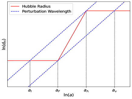
Figure 1: Hubble radius (red solid curve) and wavelength of primordial perturbation (blue dashed lines) are plotted against the scale factor in logarithmic scale.

The length $d_{H}$ will be constant during both the early inflationary epoch and the end de Sitter epoch. The initial inflationary phase ends at $a=a_{F}$ and is followed by radiation and matter dominated phases. These proceeds to another de Sitter phase of late time accelerated expansion for $a>a_{\Lambda}.$ Mathematically the two de Sitter phases can last forever. However there should exist physical cut-off length scales in both these accelerated epochs, which make the region to us be finite. Let us obtain $a_{F}$ the scale factor corresponding to which the energy densities of vacuum and radiation are equal, and after that, the radiation density will take over the vacuum density. The vacuum density in the early inflationary phase is given by equation (15). After the inflationary period, the Universe eventually make transition to radiation dominated phase, the corresponding radiation density can be expressed as in equation (16). Equating the two densities at $a=a_{F}$, we get,

$$\rho_{\Lambda_{i}}\left(\frac{1+\nu(1-\nu)\frac{H_{I}^{2}}{H_{0}^{2}}a_{F}^{4(1-\nu)}}{1+(1-\nu)\frac{H_{I}^{2}}{H_{0}^{2}}a_{F}^{4(1-\nu)}}\right)=\rho_{\Lambda_{i}}\left(\frac{(1-\nu)^{2}\frac{H_{I}^{2}}{H_{0}^{2}}a_{F}^{4(1-\nu)}}{1+(1-\nu)\frac{H_{I}^{2}}{H_{0}^{2}}a_{F}^{4(1-\nu)}}\right),$$ (19)

on simplification we get,

$$a_{F}=\left(\frac{H_{0}^{2}}{(1-2\nu)(1-\nu)H_{I}^{2}}\right)^{\frac{1}{4(1-\nu)}}.$$ (20)

We obtain the Hubble radius corresponding to $a_{F},$ using equation (10) as,

$$d_{H_{F}}=\left(\frac{2}{(1-2\nu)H_{I}^{2}}\right)^{\frac{1}{2}}.$$ (21)

Now let us go for the next important scale factor, $a_{\Lambda},$ corresponding to the switch over to the late de Sitter epoch. The energy density of radiation in the late Universe will evolves as,

$$\rho_{\gamma}(a)=\rho_{\gamma}^{0}a^{-4(1-\nu)}.$$ (22)

During this late period, the vacuum energy density can be expressed using the expression (17). At $a=a_{\Lambda}$ these two densities are equal, that is,

$$\rho_{\gamma}^{0}a^{-4(1-\nu)}=\rho_{\Lambda}^{0}+\frac{\nu}{1-\nu}\rho_{\gamma}^{0}(a^{-4(1-\nu)}-1).$$ (23)

Rearranging the above equation give rise to the scale factor $a_{\Lambda}$, as

$$a_{\Lambda}=\left(\frac{c_{0}}{(1-2\nu)[(1-\nu)H_{0}^{2}-c_{0}]}\right)^{\frac{-1}{4(1-\nu)}}.$$ (24)

The Hubble radius corresponding to the transit from radiation dominated epoch to late accelerating epoch can be obtained by substituting the above obtained expression of $a_{\Lambda}$ in equation (12), as

$$d_{H_{\Lambda}}=\left(\frac{1-2\nu}{2c_{0}}\right)^{\frac{1}{2}}.$$ (25)

The physical cut-off to both early inflation and late de Sitter epochs can be obtained as follows. During the early inflation, the Hubble radius $d_{H}$ will remain a constant due to prevailing constancy of $H$ during this epoch. On the other hand, the perturbation wavelength, $\lambda,$ grows exponentially, owing to the exponential increase of the scale factor (i.e., the wave will stretch in proportion to the scale factor). As a result, thesse perturbations will soon leave the Hubble radius. Once the Universe switched over to the radiation dominated era, the Hubble radius grows in proportion to $a^{2}$ ($d_{H}\propto a^{2}$), but the perturbation length will still grow in proportion to $a$ only (i.e. $\lambda\propto a$). If there would be no late accelrating epoch, then all the perturbation once left the Hubble sphere are eventually re-enter the Hubble sphere in the future course of evolution. But due to the late accelerated epoch, there exists some perturbation, having wavelength beyond some critical value, will never enter the Hubble radius. This critical length will naturally causes a finite extension to the early de Sitter epoch. The question is how to find this length.

Let us now consider the plot of the $\ln d_{H}$ versus $\ln a.$. The point corresponding to $a_{\Lambda}$ i.e $(\ln a_{\Lambda},\ln d_{H_{\Lambda}})$ marks the entry of the Universe into the late de Sitter epoch. The slope of the tangent to the curve at $a_{\Lambda}$, can be obtained as,

$$m=\left(\frac{dln(d_{H})}{dln(a)}\right)_{a=a_{\Lambda}}=\frac{a_{\Lambda}}{d_{H_{\Lambda}}}\left(\frac{d(d_{H})}{da}\right)_{a=a_{\Lambda}}.$$ (26)

On detailed calculation this leads to,

$$m=\frac{2(1-\nu)(H_{0}^{2}-\frac{C_{0}}{1-\nu})a_{\Lambda}^{-4(1-\nu)}}{(H_{0}^{2}-\frac{C_{0}}{1-\nu})a_{\Lambda}^{-4(1-\nu)}+\frac{C_{0}}{1-\nu}}.$$ (27)

On extending this tangent, it can be found to intersect the flat portion corresponding to the early inflation, at the point $a_{I}$ i.e.$(\ln a_{I},\ln d_{H_{I}}).$ On substituting $a_{\Lambda}^{-4(1-\nu)}$ form equation (24), it can be verified that the slope, $m=1.$ The pertubation wavelength, $\lambda\propto a,$ also have the same slope in this plane. Then it can be concluded that, perturbations leaving the Hubble sphere from beyond the location $a_{I}$ during the early inflation, will never re-enter the Hubble sphere at any time in the future. This means that any region beyond $a_{I}$ in the inflationary period would have no effect on our region, hence it can be take as a boudary which limits the past extend of inflation. Following the standard equation of the straight line, we can now deduce that,

$$a_{I}=\left(\frac{d_{H_{I}}}{d_{H_{\Lambda}}}\right)a_{\Lambda},$$ (28)

where $d_{H_{I}}$ is the Hubble radius corresponding to the early inflationary phase and it can be expressed as

$$d_{H_{I}}=\frac{1}{(1-\nu)^{\frac{1}{2}}H_{I}}.$$ (29)

We will now proceed to calculate the finite boundary of the end de Sitter epoch. The slope of the tangent at the point $(\ln a_{F},\ln d_{H_{F}})$ as,

$$n=\left(\frac{d\ln(d_{H})}{d\ln(a)}\right)_{a=a_{F}}=\frac{a_{F}}{d_{H_{F}}}\left(\frac{d(d_{H})}{da}\right)_{a=a_{F}},$$ (30)

the detailed form is,

$$n=\frac{2(1-\nu)^{2}\frac{H_{I}^{2}}{H_{0}^{2}}a_{F}^{4(1-\nu)}}{1+(1-\nu)\frac{H_{I}^{2}}{H_{0}^{2}}a_{F}^{4(1-\nu)}}.$$ (31)

The tangent will intersect the flat portion corresponding to the late de Sitter phase, at the point $a_{v}$ (i.e.$(\ln a_{v},\ln d_{H_{v}})),$ Substituting for $a_{F}$ for the previous results, it can be shown that, the slope $n=1.$ Posing similar arguements as in the previous case, the points $a_{v},$ can be taken as the finite boundary of the late de Sitter phase in the future. Equation (31) actually represents the slope of the straight line connecting the points $(\ln a_{F},\ln d_{H_{F}})$ and ($\ln a_{v},\ln d_{H_{v}}).$ Following the standard equation of the straight line, we can now deduce that,

$$a_{v}=\left(\frac{d_{H_{v}}}{d_{H_{F}}}\right)a_{F},$$ (32)

where $d_{H_{v}}$ is the Hubble radius corresponding to the late de-Sitter phase and can be expressed as

$$d_{H_{v}}=\left(\frac{1-\nu}{c_{0}}\right)^{\frac{1}{2}}.$$ (33)

From equations (28) and (32), it follows that,

$$\frac{a_{I}}{a_{F}}=\left(\frac{d_{H_{I}}}{d_{H_{\Lambda}}}\right)\left(\frac{d_{H_{v}}}{d_{H_{F}}}\right)\frac{a_{\Lambda}}{a_{v}}.$$ (34)

Substituting the equations (20), (13), (24), (25), (28), (29) in equation (34), we obtain,

$$\frac{a_{F}}{a_{I}}=\frac{a_{v}}{a_{\Lambda}}.$$ (35)

The interesting conclusion from this is that the portions $a_{I}-a_{F}$ and $a_{\Lambda}-a_{v}$ are equal. There is a middle portion in the pot corresponds to $a_{F}-a_{\Lambda},$ which represents the interim radiation/matter phase. Let us now check the relative duration of this interim phase and contrast it the duration of the first and last de Sitter epochs. From equation (14), it is clear that the slanted portion of the curve representing the Hubble radius in (Fig. 1) has a slope $2(1-\nu)$. Assuming $d_{H_{F}}$ almost equal to $d_{H_{I}}$, we can express the slope as,

$$2(1-\nu)=\frac{\ln\left(\frac{d_{H_{\Lambda}}}{d_{H_{I}}}\right)}{\ln\left(\frac{a_{\Lambda}}{a_{F}}\right)}.$$ (36)

Similarly, the slanted portion of the curve representing perturbation wavelength in (Fig. 1) has a unit slope. So we can express the slope as,

$$1=\frac{\ln\left(\frac{d_{H_{\Lambda}}}{d_{H_{I}}}\right)}{\ln\left(\frac{a_{\Lambda}}{a_{I}}\right)}.$$ (37)

combining equation (36) and (37), we obtain,

$$\left(\frac{a_{\Lambda}}{a_{F}}\right)^{1-\nu}=\frac{a_{F}}{a_{I}}.$$ (38)

From the above equation, it is clear that the portions $a_{I}-a_{F}$ and $a_{\Lambda}-a_{v}$ become equal to $a_{F}-a_{\Lambda}$ only if $\nu=0$ [29]. However the parameter $\nu$ is relatively very small, hence it can be conclude that all the three intervals are almost equal to each other.

The above proven approximate equality has an interesting significance. It turn out that the number of perturbation modes leaving the horizon during the early phase $a_{I}-a_{F}$, will re-enter the horizon during the interval $a_{F}-a_{v}$ and will exit the Hubble sphere again during $a_{\Lambda}-a_{v}.$ A perturbation of wavelength $\lambda_{p}=a/k$ (where k is the comoving wave number), crosses the Hubble radius when $\lambda_{p}(a)=H^{-1}$ or equivalently $k=aH(a)$ is satisfied. The modes having comoving wave numbers within the domain $(k,k+dk)$ cross the respective Hubble radius during the interval $(a,a+da)$. The number of modes with wave number $dk$ can be written as $dN=V_{com}d^{3}k/(2\pi)^{3}$ (where $v_{com}$ is the comoving volume). The number of modes crossing the Hubble radius during the interval $(a_{I}<a<a_{F})$ can be written as

$$N(a_{I},a_{F})=\int_{a_{I}}^{a_{F}}\frac{V_{com}k^{2}}{2\pi^{2}}\frac{dk}{da}da=\frac{2}{3\pi}\int_{H_{I}a_{I}}^{H_{F}a_{F}}\frac{d(Ha)}{Ha}=\frac{2}{3\pi}\ln\left(\frac{H_{F}a_{F}}{H_{I}a_{I}}\right)$$ (39)

Substituting for $a_{I}$ form equation (28), gives

$$N(a_{I},a_{F})=\frac{2}{3\pi}\ln\left(\frac{H_{F}a_{F}}{H_{\Lambda}a_{\Lambda}}\right)$$ (40)

The RHS of the above equation is $N(a_{F},a_{\Lambda})$ the number modes crossing the Hubble radius of the radiation dominated era. Thus the number of modes leaving the horizon during early inflationary period will re-enter the radiation dominated era. Now substitute for $a_{F}$ in equation (40) from equation (32) we obtain

$$N(a_{I},a_{F})=\frac{2}{3\pi}\ln\left(\frac{H_{v}a_{v}}{H_{\Lambda}a_{\Lambda}}\right)$$ (41)

which in turn equal to $N(a_{\Lambda},a_{v}).$ From equation (40) and equation (41), we obtain that the number of perturbations modes leaving the Hubble radius of the early inflationary phase, subsequently re-enter the radiation pahse and finally exit the end de Sitter epoch corrsponding to the late acceleration, hence

$$N(a_{I},a_{F})=N(a_{F},a_{\Lambda})=N(a_{\Lambda},a_{v}).$$ (42)

This otherwise implies that, $\left(\frac{H_{F}a_{F}}{H_{\Lambda}a_{\Lambda}}\right)=\left(\frac{H_{v}a_{v}}{H_{\Lambda}a_{\Lambda}}\right),$ which in turn equal to $\left(\frac{H_{F}a_{F}}{H_{I}a_{I}}\right).$ This equality, however doesn’t implies the equality of the intervals in the scale factor, especially in the case of the interim radiation (or matter) dominated epoch. The number of modes crossing the Hubble radii in subsequent epochs is thus a conserved quantiy and let it be denoted by $N_{c}$ for our Universe. In the following we evaluate this quantiy. Consider the radiation dominated epoch. The number of modes crossing the Hubble radius during the interval $a_{F}<a<a_{\Lambda}$ can be written as,

$$N_{c}=\frac{2}{3\pi}\ln\left(\frac{H_{F}a_{F}}{H_{\Lambda}a_{\Lambda}}\right)=\frac{2}{3\pi}\ln\left(\frac{d_{H_{\Lambda}}a_{F}}{d_{H_{F}}a_{\Lambda}}\right),$$ (43)

Substituting equation (21), (20), (24) and (25) in equation (43), we obtain

$$\begin{split}N_{c}=\frac{2}{3\pi}\ln\left[\frac{(1-2\nu)H_{I}}{2\sqrt{c_{0}}}\left(\frac{\sqrt{c_{0}}}{(1-2\nu)(1-\nu)H_{I}\left(\sqrt{1-(\frac{c_{0}}{(1-\nu)H_{0}^{2}})}\right)}\right)^{\frac{1}{2(1-\nu)}}\right]\end{split}$$ (44)

an on simplification, we arrive at,

$$\begin{split}N_{c}\sim\frac{(1-2\nu)}{3\pi(1-\nu)}\ln\left(\frac{(1-2\nu)H_{I}}{\sqrt{c_{0}}}\right)-\frac{2}{3\pi}\ln(2)-\frac{1}{3\pi(1-\nu)}\ln(1-\nu)\end{split}$$ (45)

The second and third term in equation (45) are negligible small compared to first term, hence we obtain

$$\begin{split}N_{c}\sim\frac{(1-2\nu)}{3\pi(1-\nu)}\ln\left(\frac{(1-2\nu)H_{I}}{\sqrt{c_{0}}}\right).\end{split}$$ (46)

Here $H_{I}$ is the Hubble parameter of the initial de Sitter Universe, and $c_{0}$ represents the Hubble parameter corresponds to the late de Sitter Universe. The model parameter $\nu\leq 10^{-3}$ and if it assumed to be negligibly small, then $N_{c}\sim(1/3\pi)\ln\left(\frac{H_{I}}{\sqrt{c_{0}}}\right).$ Assuming the standard values, $H_{I}\sim 10^{14}$ GeV and $\sqrt{c_{0}}\sim 10^{-42}$ GeV, it can be shown that, $N_{c}\sim 4\pi.$ Here we have expressed the numerical value by retaining $\pi$ because we have that in the denominator of the arguement of the logarithm.

4 Conclusions

In this work, we have derived an analytical solution for the Hubble parameter for the complete background evolution of the Universe; from the early inflation to late de Sitter phase using the running vacuum model of the dark energy proposed by Sola and others. The general form of the Hubble parameter is suitably reduced to the one which corresponds to the subsequent phases in the evolution of the Universe, the early inflation, interim radiation (matter), and end de Sitter epochs through a late accelerated phase. The Universe, with evolution as shown in figure (1) having two distinct de Sitter epochs, one during the inflation and the other during the late time acceleration. Both of these epochs can be extended indefinitely into the past and future with a constant Hubble radius. Nevertheless, there are physical processes that limit the physically relevant region of these two epochs. Since the Hubble radius flattens out when $a>a_{\Lambda}$, the perturbations with wavelengths larger than a critical value will never re-enter the Hubble radius, which we imply a physical boundary of this de Sitter epoch. This otherwise implies that only those perturbations that left the early inflationary period during $a_{I}<a<a_{F}$ are feasible, which in turn determine the early de Sitter’s finite boundary epoch. We found that the resepctive scale factors will satisfy a relation, $(a_{F}/a_{I})=(a_{v}/a_{\Lambda}).$ The transition between the two de Sitter phases is through a radiation dominated phase, giving way to a very late time matter-dominated phase. It is, however, evident that the matter-dominated epoch is not much significant since it quickly gives way to the second de Sitter phase dominated by the cosmological constant. Hence we considered only the radiation epoch as the transient phase. On analyzing the evolution of this interim epoch, we found the scale factors ratio, which can equate with the previously mentioned ratio is $(a_{\Lambda}/a_{F})^{1-\nu}.$ One may note at this juncture that the slanted portion in figure (1), which represents the evolution of the interim phase, has a slope of 2$(1-\nu).$

The perturbation modes which exit the Hubble radius during $a_{I}-a_{F}$ re-enter the Hubble radius during $a_{F}-a_{\Lambda}$ and again exit during $a_{\Lambda}-a_{v}.$ We obtained this conserved number of modes and is approximately $N_{c}\sim(1/3\pi)\ln\left(\frac{H_{I}}{\sqrt{c_{0}}}\right).$ We expect that this constant number may have further insights into the connection between the early inflationary epoch and the end de Sitter epoch, about which more work is needed.

References

- [1] J. D. Bjorken, “Cosmology and the standard model,” Physical Review D, vol. 67, no. 4, p. 043508, 2003.
- [2] N. A. Bahcall, J. P. Ostriker, S. Perlmutter, and P. J. Steinhardt, “The cosmic triangle: Revealing the state of the universe,” 1999.
- [3] E. J. Copeland, M. Sami, and S. Tsujikawa, “Dynamics of dark energy,” International Journal of Modern Physics D, vol. 15, no. 11, pp. 1753–1935, 2006.
- [4] S. Perlmutter, G. Aldering, G. Goldhaber, R. A. Knop, P. Nugent, P. G. Castro, S. Deustua, S. Fabbro, A. Goobar, D. E. Groom, I. M. Hook, A. G. Kim, M. Y. Kim, J. C. Lee, N. J. Nunes, R. Pain, C. R. Pennypacker, R. Quimby, C. Lidman, R. S. Ellis, M. Irwin, R. G. McMahon, P. Ruiz-Lapuente, N. Walton, B. Schaefer, B. J. Boyle, A. V. Filippenko, T. Matheson, A. S. Fruchter, N. Panagia, H. J. M. Newberg, W. J. Couch, and T. S. C. Project, “Measurements of and from 42 High-Redshift Supernovae,” apj, vol. 517, pp. 565–586, June 1999.
- [5] A. G. Riess, A. V. Filippenko, P. Challis, A. Clocchiatti, A. Diercks, P. M. Garnavich, R. L. Gilliland, C. J. Hogan, S. Jha, R. P. Kirshner, B. Leibundgut, M. M. Phillips, D. Reiss, B. P. Schmidt, R. A. Schommer, R. C. Smith, J. Spyromilio, C. Stubbs, N. B. Suntzeff, and J. Tonry, “Observational Evidence from Supernovae for an Accelerating Universe and a Cosmological Constant,” apj, vol. 116, pp. 1009–1038, Sept. 1998.
- [6] G. Papagiannopoulos, P. Tsiapi, S. Basilakos, and A. Paliathanasis, “Dynamics and cosmological evolution in -varying cosmology,” The European Physical Journal C, vol. 80, p. 55, Jan 2020.
- [7] J. Sola, “Cosmological constant and vacuum energy: old and new ideas,” J. Phys. Conf. Ser., vol. 453, p. 012015, 2013.
- [8] S. Weinberg, “The cosmological constant problem,” Reviews of modern physics, vol. 61, no. 1, p. 1, 1989.
- [9] T. Padmanabhan, “Cosmological constant—the weight of the vacuum,” Physics Reports, vol. 380, no. 5-6, pp. 235–320, 2003.
- [10] J. Lima, S. Basilakos, and J. Solà, “Expansion history with decaying vacuum: a complete cosmological scenario,” Monthly Notices of the Royal Astronomical Society, vol. 431, no. 1, pp. 923–929, 2013.
- [11] J. S. Peracaula, J. de Cruz Pérez, and A. Gómez-Valent, “Dynamical dark energy vs. = const in light of observations,” EPL (Europhysics Letters), vol. 121, no. 3, p. 39001, 2018.
- [12] A. Gomez-Valent, J. Sola, and S. Basilakos, “Dynamical vacuum energy in the expanding universe confronted with observations: a dedicated study,” Journal of Cosmology and Astroparticle Physics, vol. 2015, no. 01, p. 004, 2015.
- [13] J. Sola, A. Gomez-Valent, and J. de Cruz Pérez, “Hints of dynamical vacuum energy in the expanding universe,” The Astrophysical Journal Letters, vol. 811, no. 1, p. L14, 2015.
- [14] P. George and T. K. Mathew, “Holographic ricci dark energy as running vacuum,” Modern Physics Letters A, vol. 31, no. 13, p. 1650075, 2016.
- [15] R. C. Nunes, “Connecting inflation with late cosmic acceleration by particle production,” Int. J. Mod. Phys. D, vol. 25, no. 06, p. 1650067, 2016.
- [16] S. Fay, “From inflation to late time acceleration with a decaying vacuum coupled to radiation or matter,” Phys. Rev. D, vol. 89, p. 063514, 2014.
- [17] P. Tsiapi and S. Basilakos, “Testing dynamical vacuum models with cmb power spectrum from planck,” Monthly Notices of the Royal Astronomical Society, vol. 485, no. 2, pp. 2505–2510, 2019.
- [18] L. Amendola, “Coupled quintessence,” Physical Review D, vol. 62, no. 4, p. 043511, 2000.
- [19] S. Del Campo, R. Herrera, and D. Pavón, “Toward a solution of the coincidence problem,” Physical Review D, vol. 78, no. 2, p. 021302, 2008.
- [20] G. S. Sharov, S. Bhattacharya, S. Pan, R. C. Nunes, and S. Chakraborty, “A new interacting two-fluid model and its consequences,” Monthly Notices of the Royal Astronomical Society, vol. 466, no. 3, pp. 3497–3506, 2017.
- [21] S. Nojiri and S. D. Odintsov, “Modified gravity with negative and positive powers of curvature: Unification of inflation and cosmic acceleration,” Phys. Rev. D, vol. 68, p. 123512, Dec 2003.
- [22] S. Nojiri and S. D. Odintsov, “Modified gravity with negative and positive powers of curvature: Unification of inflation and cosmic acceleration,” physical Review D, vol. 68, no. 12, p. 123512, 2003.
- [23] J. Solà and A. Gómez-Valent, “The cosmology: From inflation to dark energy through running ,” Int. J. Mod. Phys. D, vol. 24, p. 1541003, 2015.
- [24] I. L. Shapiro and J. Sola, “The scaling evolution of the cosmological constant,” Journal of High Energy Physics, vol. 2002, no. 02, p. 006, 2002.
- [25] J. Sola, “Cosmologies with a time dependent vacuum,” in Journal of Physics: Conference Series, vol. 283, p. 012033, IOP Publishing, 2011.
- [26] J. Sola, “Cosmological constant and vacuum energy: old and new ideas,” in Journal of Physics: Conference Series, vol. 453, p. 012015, IOP Publishing, 2013.
- [27] J. Solà, “Vacuum energy and cosmological evolution,” in AIP Conference Proceedings, vol. 1606, pp. 19–37, American Institute of Physics, 2014.
- [28] M. V. John and K. B. Joseph, “Generalized chen-wu type cosmological model,” Physical Review D, vol. 61, no. 8, p. 087304, 2000.
- [29] T. Padmanabhan, “Emergent perspective of gravity and dark energy,” Research in Astronomy and Astrophysics, vol. 12, pp. 891–916, aug 2012.
- [30] I. L. Shapiro, J. Sola, and H. Štefančić, “Running g and at low energies from physics at mx: possible cosmological and astrophysical implications,” Journal of cosmology and astroparticle physics, vol. 2005, no. 01, p. 012, 2005.
- [31] H. Padmanabhan and T. Padmanabhan, “Cosmin: The solution to the cosmological constant problem,” International Journal of Modern Physics D, vol. 22, no. 12, p. 1342001, 2013.
- [32] T. Padmanabhan and H. Padmanabhan, “Cosmological constant from the emergent gravity perspective,” International Journal of Modern Physics D, vol. 23, no. 06, p. 1430011, 2014.
- [33] T. Padmanabhan and H. Padmanabhan, “Solution to the cosmological constant problem,” tech. rep., 2013.