Score-oriented loss (SOL) functions

Abstract

Loss functions engineering and the assessment of forecasting performances are two crucial and intertwined aspects of supervised machine learning. This paper focuses on binary classification to introduce a class of loss functions that are defined on probabilistic confusion matrices and that allow an automatic and a priori maximization of the skill scores. The performances of these loss functions are validated during the training phase of two experimental forecasting problems, thus showing that the probability distribution function associated with the confusion matrices significantly impacts the outcome of the score maximization process.

68T05, 68Q32, 92B20, 65K10

1 Introduction

Neural networks (NNs) are well-established models in the field of machine learning. Given their flexibility and capability in addressing complex tasks where a large amount of data is at the disposal, deep NNs are the state-of-art of many classification issues, including image recognition [Pelletier19], speech analysis [Deng13] and medical diagnostics [kermany2018identifying]; for a detailed treatment of various NNs architectures, as well as of related deep learning topics, we refer e.g. to [Goodfellow16].

In general, a network depends on a set of weights that are optimized in such a way that an objective function, made of a loss function and a regularization term, is minimized [girosi1995regularization]. Loss functions measure the possible discrepancy between the NN prediction and a label encoding the information about the event occurrence. Loss design is a crucial aspect of machine learning theory [rosasco2004loss] and, over the years, several functions have been proposed, typically with the aim of accounting for the specific properties of the problem under analysis [Janocha16, Lin17, Liu16, Zhu20]. Among these choices, Cross Entropy (CE) and its generalizations [Good52, Lu19, Zhang18] possess a solid theoretical background that can be traced back to information theory, they being related to the notions of entropy and Kullback-Leibler divergence, and their minimization corresponds to the maximization of the likelihood under a Bernoulli model (see e.g. [Murphy12, Section 2.8]).

While the network is optimized by minimizing a certain loss, the classification results are then evaluated by considering some well-established metrics or skill scores, which are often chosen according to the particular task and derived from the elements of the so-called confusion matrix (CM). Although loss minimization and score maximization are two intertwined concepts, yet a direct maximization of a score during the training of the network is to be avoided, since the score is typically a discontinuous function with respect to the predictions given by the model. Therefore, other strategies have been taken into consideration.

For example, in [Huang19] the authors propose an adaptive loss alignment with respect to the evaluation metric via a reinforcement learning approach. A loss function that approximates the 0-1 loss is proposed in [Singh10]. In [Rezatofighi19], a loss that generalizes the Jaccard index is discussed for object detection issues. In order to address the lack of regularity of the score, fuzzy or probabilistic confusion matrices have been examined e.g. in [Koco13], where the minimization of the off-diagonal elements of a probabilistic confusion matrix is considered; in [Wang13], where a confusion entropy metric is constructed; and in [Trajdos16], where local fuzzy CMs have been employed.

This fuzzy/probabilistic approach was inspirational for the framework introduced in the present paper, which also presents similarities with the main idea investigated in [Ohsaki17] in the context of kernel logistic regression, and which has to be intended as the theoretically-founded generalization of the approach carried out, e.g., in [Zhang17]. Indeed, our study addresses the problem of filling the gap between score maximization and loss minimization by constructing a class of Score-Oriented Loss (SOL) functions out of a classical CM. The main idea consists in treating the threshold that influences the entries of the confusion matrix not as a fixed value, but as a random variable. Therefore, by considering the expected value of the matrix, we build losses that are indeed derivable with respect to the weights of the model. Furthermore, we theoretically motivate and then numerically show that the probability distribution chosen a priori for the threshold severely influences the outcome of the a posteriori score maximization. More in details, the optimal threshold is very likely to be placed in the concentration areas of the a priori distribution. As a consequence, using a SOL function related to a certain skill score, we automatically obtain an optimized value without performing any further a posteriori procedure.

The paper is organized as follows. In Section 2, starting from a classical confusion matrix, we construct the theoretical foundation of our SOL functions and we investigate their properties. Section 3 describes two possible choices for the probability distribution associated to the threshold and illustrates their application to two experimental forecasting problems. Finally, our conclusions are offered in Section LABEL:sec:conclusions.

2 Construction and properties of score-oriented losses

Let $\Omega\subset\mathbb{R}^{m}$ and let $\mathcal{X}\subset\Omega$ be a set of data, $m\in\mathbb{N}_{\geq 1}$. Let $\mathcal{Y}$ be a finite set of $d$ labels or classes to be learned, where $d\in\mathbb{N}_{\geq 2}$ and the labels (or classes) are integer encoded or one-hot encoded in practice [Harris13]. Suppose that each element in $\mathcal{X}$ is uniquely assigned to a class in $\mathcal{Y}$. Then, the supervised classification problem, where $d=2$, consists of constructing a function $g$ on $\Omega$ by learning from the labeled data set $\mathcal{X}$, in such a way that $g$ models the data-label relation between elements in $\Omega$ and labels in $\mathcal{Y}$. In order to achieve such result, one usually defines a loss function $\ell(g(\bm{x}),y)$ that measures the possible discrepancy between the prediction $g(\bm{x})$ given by the model, $\bm{x}\in\mathcal{X}$, and its true label $y\in\mathcal{Y}$. In this view, an NN builds the function $g$ by minimizing the loss on the training set $X$, as well as focusing on its generalization capability when predicting possible unseen test samples in $\Omega$.

More specifically, the network produces the output

$$\hat{y}(\bm{x},\bm{w})\coloneqq(\sigma\circ h)(\bm{x},\bm{w})\in[0,1],\;\bm{x}\in\Omega,$$

where $h(\bm{x},\bm{w})$ denotes the outcome of the input and hidden layers, being $\bm{w}$ the vector (matrix) of weight parameters, and $\sigma$ is the sigmoid activation function defined as $\sigma(h)=(1+e^{-h})^{-1}$.

During the training procedure, the weights of the network are adjusted via backpropagation in such a way that a certain objective function is minimized, i.e. we consider the following minimization problem

(1) $$\min_{\bm{w}}\ell(\hat{y}(\bm{x},\bm{w}),y)+\lambda R(\bm{w}),\;\bm{x}\in\Omega,$$

where $\ell$ is a loss function and $R(\bm{w})$ is a possible regularization term that is controlled by a parameter $\lambda\in\mathbb{R}_{>0}$. The outcomes of this regression problem can be clustered by means of some thresholding process in order to construct a classifier whose predictive effectiveness is assessed by means of specific skill scores. We now introduce a one-parameter family of CMs from which we will derive a set of probabilistic skill scores. This approach will allow the introduction of a corresponding set of probabilistic loss functions and, accordingly, an a priori optimization of the scores.

2.1 Confusion matrices with probabilistic thresholds

Let us consider a batch of predictions-labels $\mathcal{S}=\mathcal{S}_{n}(\bm{w})=\{(\hat{y}(\bm{x}_{i},\bm{w}),y_{i})\}_{i=1,\dots,n}$, where $y_{i}\in\{0,1\}$ is the true label associated to the element $\bm{x}_{i}\in\mathcal{X}$ and $\hat{y}(\bm{x}_{i},\bm{w})\in[0,1]$ is the prediction for $\bm{x}_{i}$ given by the model. Furthermore, let $n^{+}$ and $n^{-}$ be the number of elements in $\mathcal{S}_{n}(\bm{w})$ whose true class $y_{i}$, $i=1,\dots,n$, is the positive ($\{y=1\}$) or the negative ($\{y=0\}$), respectively. Therefore, $n^{+}+n^{-}=n$.

Let $\tau\in\mathbb{R},\;\tau\in(0,1),$ and let

$$\mathbbm{1}_{x}(\tau)=\mathbbm{1}_{\{x>\tau\}}=\begin{dcases}0&\textrm{if }x\leq\tau,\\ 1&\textrm{if }x>\tau,\end{dcases}\quad x\in(0,1),$$

be the indicator function. The classical confusion matrix is defined as

$$\mathrm{CM}(\tau)=\mathrm{CM}(\tau,\mathcal{S}_{n}(\bm{w}))=\begin{pmatrix}\mathrm{TN}(\tau,\mathcal{S}_{n}(\bm{w}))&\mathrm{FP}(\tau,\mathcal{S}_{n}(\bm{w}))\\ \mathrm{FN}(\tau,\mathcal{S}_{n}(\bm{w}))&\mathrm{TP}(\tau,\mathcal{S}_{n}(\bm{w}))\end{pmatrix},$$

where the elements are

(2) $$\begin{split}&\mathrm{TN}(\tau,\mathcal{S}_{n}(\bm{w}))=\sum_{i=1}^{n}{(1-y_{i})\mathbbm{1}_{\{\hat{y}(\bm{x}_{i},\bm{w})<\tau\}}},\;\mathrm{TP}(\tau,\mathcal{S}_{n}(\bm{w}))=\sum_{i=1}^{n}{y_{i}\mathbbm{1}_{\{\hat{y}(\bm{x}_{i},\bm{w})>\tau\}}},\vspace{5pt}\\ &\mathrm{FP}(\tau,\mathcal{S}_{n}(\bm{w}))=\sum_{i=1}^{n}{(1-y_{i})\mathbbm{1}_{\{\hat{y}(\bm{x}_{i},\bm{w})>\tau\}}},\;\mathrm{FN}(\tau,\mathcal{S}_{n}(\bm{w}))=\sum_{i=1}^{n}{y_{i}\mathbbm{1}_{\{\hat{y}(\bm{x}_{i},\bm{w})<\tau\}}}.\end{split}$$

In what follows, we let $\tau$ be a continuous random variable whose probability density function (pdf) $f$ is supported in $[a,b]\subseteq[0,1]$, $a,b\in\mathbb{R}$. Furthermore, we denote as $F$ the cumulative density function (cdf)

$$F(x)=\int_{a}^{x}{f(\xi)\mathrm{d}\xi},\quad x\leq b.$$

We recall that

$$\mathbb{E}_{\tau}[\mathbbm{1}_{x}(\tau)]=\int_{a}^{b}{\mathbbm{1}_{\{x>\xi\}}f(\xi)\mathrm{d}\xi}=\int_{a}^{x}{f(\xi)\mathrm{d}\xi}=F(x).$$

This leads to the following definition.

Definition 2.1.

Let $\mathcal{S}_{n}(\bm{w})$ be a batch of predictions-labels and let $\mathrm{CM}(\tau,\mathcal{S}_{n}(\bm{w}))$ be a confusion matrix as defined in (2). Moreover, let $\tau$ be a continuous random variable on $(0,1)$ with cdf $F$. We define the expected confusion matrix as

$$\overline{\mathrm{CM}}_{F}=\overline{\mathrm{CM}}_{F}(\mathcal{S}_{n}(\bm{w}))=\begin{pmatrix}\overline{\mathrm{TN}}_{F}(\mathcal{S}_{n}(\bm{w}))&\overline{\mathrm{FP}}_{F}(\mathcal{S}_{n}(\bm{w}))\\ \overline{\mathrm{FN}}_{F}(\mathcal{S}_{n}(\bm{w}))&\overline{\mathrm{TP}}_{F}(\mathcal{S}_{n}(\bm{w}))\end{pmatrix},$$

where

(3) $$\begin{split}&\overline{\mathrm{TN}}_{F}(\mathcal{S}_{n}(\bm{w}))=\sum_{i=1}^{n}{(1-y_{i})(1-F(\hat{y}(\bm{x}_{i},\bm{w})))},\;\overline{\mathrm{TP}}_{F}(\mathcal{S}_{n}(\bm{w}))=\sum_{i=1}^{n}{y_{i}F(\hat{y}(\bm{x}_{i},\bm{w}))},\vspace{5pt}\\ &\overline{\mathrm{FP}}_{F}(\mathcal{S}_{n}(\bm{w}))=\sum_{i=1}^{n}{(1-y_{i})F(\hat{y}(\bm{x}_{i},\bm{w}))},\vspace{5pt}\;\overline{\mathrm{FN}}_{F}(\mathcal{S}_{n}(\bm{w}))=\sum_{i=1}^{n}{y_{i}(1-F(\hat{y}(\bm{x}_{i},\bm{w})))}.\end{split}$$

Remark 2.2.

We observe that $\overline{\mathrm{CM}}_{F}$ is indeed the expected value of the matrix $\mathrm{CM}(\tau)$ with respect to $\tau$, meaning that

(4) $$\mathbb{E}_{\tau}[\mathrm{CM}(\tau)]\coloneqq\begin{pmatrix}\mathbb{E}_{\tau}[\mathrm{TN}(\tau,\mathcal{S}_{n}(\bm{w}))]&\mathbb{E}_{\tau}[\mathrm{FP}(\tau,\mathcal{S}_{n}(\bm{w}))]\\ \mathbb{E}_{\tau}[\mathrm{FN}(\tau,\mathcal{S}_{n}(\bm{w}))]&\mathbb{E}_{\tau}[\mathrm{TP}(\tau,\mathcal{S}_{n}(\bm{w}))]\end{pmatrix}=\overline{\mathrm{CM}}_{F}.$$

Moreover, the sum by rows is preserved, that is for any $\tau\in(0,1)$

$$\big{\lVert}\overline{\mathrm{CM}}_{F}(\mathcal{S}_{n}(\bm{w}))\big{\lVert}_{\infty}=\big{\lVert}\mathrm{CM}(\tau,\mathcal{S}_{n}(\bm{w}))\big{\lVert}_{\infty}=\max\{n^{-},n^{+}\}.$$

Hence, all considered matrices are contained in the set

(5) $$\mathcal{C}(\mathcal{S}_{n})\coloneqq\{\mathrm{A}\in\mathcal{M}^{+}_{2}\>|\>\mathrm{A}_{11}+\mathrm{A}_{12}=n^{-},\;\mathrm{A}_{21}+\mathrm{A}_{22}=n^{+}\},$$

where $\mathrm{A}=(\mathrm{A}_{ij})_{i,j=1,2}$ and $\mathcal{M}^{+}_{2}$ is the set of $2\times 2$ positive-valued matrices.

Therefore, we can prove the following results by considering well-known concentration inequalities:

Proposition 2.3.

Let $\mathcal{S}_{n}\coloneqq\mathcal{S}_{n}(\bm{w})$ be a batch of predictions-labels, $n\in\mathbb{N}$, and let $\tau$ be a continuous random variable on $(0,1)$ with cdf $F$. Then, letting $\mathrm{N}\in\{\mathrm{TN},\mathrm{FP}\}$, $\mathrm{P}\in\{\mathrm{TP},\mathrm{FN}\}$ and $\varepsilon>0$, we have

(6) $$\begin{split}&\mathbb{P}(|\mathrm{N}(\tau,\mathcal{S}_{n})-\overline{\mathrm{N}}_{F}(\mathcal{S}_{n})|\geq\varepsilon)\leq 2\>\mathrm{exp}\bigg{(}-\frac{2\varepsilon^{2}}{(n^{-})^{2}}\bigg{)},\\ &\mathbb{P}(|\mathrm{P}(\tau,\mathcal{S}_{n})-\overline{\mathrm{P}}_{F}(\mathcal{S}_{n})|\geq\varepsilon)\leq 2\>\mathrm{exp}\bigg{(}-\frac{2\varepsilon^{2}}{(n^{+})^{2}}\bigg{)}.\end{split}$$

Moreover, denoting as $\mathrm{tr}(\mathrm{CM})=\mathrm{TN}+\mathrm{TP}$ the trace of the confusion matrix, we get

(7) $$\mathbb{P}(|\mathrm{tr}(\mathrm{CM}(\tau,\mathcal{S}_{n}))-\mathrm{tr}(\overline{\mathrm{CM}}_{F}(\mathcal{S}_{n}))|\geq\varepsilon)\leq 2\>\mathrm{exp}\bigg{(}-\frac{2\varepsilon^{2}}{(n^{-})^{2}+(n^{+})^{2}}\bigg{)}.$$

Proof 2.4.

In order to prove (6) it is sufficient to consider the McDiarmid’s inequality (see e.g. [ShaweTaylor04, Theorem 4.5, p.88]) and to observe that

$$\sup_{\tau_{1},\tau_{2}\in(0,1)}{|\mathrm{N}(\tau_{1},\mathcal{S}_{n})-\mathrm{N}(\tau_{2},\mathcal{S}_{n})|}=n^{-},\;\sup_{\tau_{1},\tau_{2}\in(0,1)}{|\mathrm{P}(\tau_{1},\mathcal{S}_{n})-\mathrm{P}(\tau_{2},\mathcal{S}_{n})|}=n^{+}.$$

Then, we can apply the Hoeffding’s inequality [Hoeffding63] to $\mathrm{TN}(\tau,\mathcal{S}_{n})+\mathrm{TP}(\tau,\mathcal{S}_{n})$, thus obtaining (7).

2.2 Derived scores and loss functions

A skill score is a function mapping the space of confusion matrices onto $\mathbb{R}$. In the classical setting, the skill score is denoted as $s:M_{2,2}(\mathbb{N})\rightarrow\mathbb{R}$ and is constructed on $\mathrm{CM}(\tau,\mathcal{S}_{n}(\bm{w}))$ for a fixed value of $\tau\in(0,1)$. In the case of confusion matrices with probabilistic threshold, the score explicitly depends on the cumulative distribution function $F$ adopted and is therefore denoted as ${\overline{s}}_{F}:M_{2,2}(\mathbb{R})\rightarrow\mathbb{R}$. In this latter case, we can introduce a class of Score-Oriented Loss (SOL) functions as follows.

Definition 2.5.

Let $\mathcal{S}_{n}(\bm{w})$ be a batch of predictions-labels and let $s(\tau,\mathcal{S}_{n}(\bm{w}))=s(\tau)$ be a score calculated upon $\mathrm{CM}(\tau,\mathcal{S}_{n}(\bm{w}))$, $\tau\in(0,1)$. Indicating with ${\overline{s}}_{F}(\mathcal{S}_{n}(\bm{w}))={\overline{s}}_{F}$ the score $s$ calculated upon $\overline{\mathrm{CM}}_{F}(\mathcal{S}_{n}(\bm{w}))$, a Score-Oriented Loss (SOL) function related to $s$ is defined as

$$\ell_{\overline{s}}(F,\mathcal{S}_{n}(\bm{w})))\coloneqq-{\overline{s}}_{F}(\mathcal{S}_{n}(\bm{w}))).$$

As an example, taking the accuracy score

$$\textrm{acc}=\frac{\textrm{TP}+\textrm{TN}}{\textrm{TP}+\textrm{TN}+\textrm{FP}+\textrm{FN}},$$

we get

$$\begin{split}\overline{\textrm{acc}}_{F}(\mathcal{S}_{n}(\bm{w})))&\coloneqq\frac{\sum_{i=1}^{n}{y_{i}F(\hat{y}(\bm{x}_{i},\bm{w}))+(1-y_{i})(1-F(\hat{y}(\bm{x}_{i},\bm{w})))}}{n}\end{split}$$

and then the loss function $\ell_{\overline{\textrm{acc}}}(F,\mathcal{S}_{n}(\bm{w}))\coloneqq-\overline{\textrm{acc}}_{F}(\mathcal{S}_{n}(\bm{w})))$.

Remark 2.6.

By setting $0/0\coloneqq 0$ and by virtue of the fundamental theorem of calculus, we observe that $\ell_{\overline{s}}$ is derivable with respect to the weights vector $\bm{w}$, which is a fundamental property for its usage as loss function.

We now prove the following

Theorem 2.7.

Let $\mathcal{S}_{n}\coloneqq\mathcal{S}_{n}(\bm{w})$ be a batch of predictions-labels, $n\in\mathbb{N}$, and let $\tau$ be a continuous random variable on $(0,1)$ with cdf $F$. Then, if $s$ is linear with respect to the entries of the confusion matrix, we have

(8) $$\mathbb{E}_{\tau}[s(\tau,\mathcal{S}_{n})]=\overline{s}_{F}(\mathcal{S}_{n}).$$

Moreover, letting $\mathrm{supp}(s(\tau,\mathcal{S}_{n}))=[a,b]$, $a,b\in\mathbb{R}$, $a<b$, and $\varepsilon>0$, we obtain

(9) $$\mathbb{P}(|s(\tau,\mathcal{S}_{n})-\overline{s}_{F}(\mathcal{S}_{n})|\geq\varepsilon)\leq 2\>\mathrm{exp}\bigg{(}-\frac{2\varepsilon^{2}}{(b-a)^{2}}\bigg{)}.$$

Proof 2.8.

Due to the linearity of the expected value, the results in Proposition 2.3 imply (8). As a consequence, the McDiarmid’s inequality can be applied in order to obtain (9).

Remark 2.9.

Suppose that the score is not linear with respect to the entries of the vectorized confusion matrix $\mathrm{vec}(\mathrm{CM}(\tau))=(\mathrm{TN}(\tau),\mathrm{FP}(\tau),\mathrm{FN}(\tau),\mathrm{TP}(\tau))$. By looking at the scores $s$ and $\overline{s}_{F}$ as functions of $\mathrm{vec}(\mathrm{CM}(\tau))$, i.e. $s(\tau)=s(\mathrm{vec}(\mathrm{CM}(\tau)))$ and $\overline{s}_{F}=s(\mathrm{vec}(\overline{\mathrm{CM}}_{F}))$, we have the Taylor approximation (see e.g. [Benaroya05])

$$s(\mathrm{vec}(\mathrm{CM}(\tau)))\approx s(\mathrm{vec}(\overline{\mathrm{CM}}_{F}))+\sum_{|\bm{\alpha}|\geq 1}{\frac{D^{\bm{\alpha}}s(\mathrm{vec}(\overline{\mathrm{CM}}_{F}))}{\bm{\alpha}!}(\mathrm{vec}(\mathrm{CM}(\tau)-\overline{\mathrm{CM}}_{F}))^{\bm{\alpha}}},$$

which implies

$$\mathbb{E}_{\tau}[s(\tau)]\approx\overline{s}_{F}+\sum_{|\bm{\alpha}|\geq 1}{\frac{D^{\bm{\alpha}}\overline{s}_{F}}{\bm{\alpha}!}\mathbb{E}_{\tau}[(\mathrm{vec}(\mathrm{CM}(\tau)-\overline{\mathrm{CM}}_{F}))^{\bm{\alpha}}]},$$

where $\bm{\alpha}\in\mathbb{N}^{4}$ denotes the classical multi-index notation.

Recalling (1), let $T(\bm{w})\coloneqq\ell(\mathcal{S}(\bm{w}))+\lambda R(\bm{w})$ be the target function to minimize during the training of the network, where $\ell$ is a generic loss function. When performing a posteriori maximization of a score $s$, letting $\bm{w}^{\star}=\operatorname*{argmin}_{\bm{w}}T(\bm{w})$, we compute

$$\max_{\tau\in(0,1)}s(\tau,\mathcal{S}(\bm{w}^{\star})).$$

In our setting with SOL functions, in view of Definition 2.5 and Remark 2.9, the training minimization problem results in

$$\min_{\bm{w}}\ell_{\overline{s}}(F,\mathcal{S}(\bm{w})))+\lambda R(\bm{w})\approx\max_{\bm{w}}\mathbb{E}_{\tau}[s(\tau,\mathcal{S}(\bm{w}))]-\lambda R(\bm{w}),$$

where the equality is achieved under the assumptions of Theorem 2.7. Therefore, the maximization of the expected value of the score is included in the training process. Moreover, we observe that while a direct maximization of the score $s(\tau^{\star},\mathcal{S}(\bm{w}))$ for a fixed $\tau^{\star}\in(0,1)$ is not possible due to the lack of derivability, this procedure can be approximated by considering for $\tau$ a probability distribution highly concentrated around the mean value $\tau^{\star}$. In Section 3, we review two different probability distributions that express different concentration properties.

The following result concerns the mean absolute deviation (mad) [Geary35] of a Lipschitz continuous score $s$ from its expected value $\overline{s}_{F}$.

Theorem 2.10.

Let $\mathcal{S}_{n}$ be a batch of predictions-labels, $n\in\mathbb{N}$, and let $\tau$ be a continuous random variable on $(0,1)$ with cdf $F$. Assume that $s$ is a Lipschitz continuous function with respect to the entries of $\mathrm{CM}(\tau,\mathcal{S}_{n})$ on the set $\mathcal{C}(\mathcal{S}_{n})$. Then,

$$\mathbb{E}_{\tau}[|s(\tau,\mathcal{S}_{n})-{\overline{s}}_{F}(\mathcal{S}_{n})|]\leq\frac{1}{2}\>K_{s}(J_{F}+\mathrm{mad}_{\tau}[\mathrm{TN}(\tau)]+\mathrm{mad}_{\tau}[\mathrm{TP}(\tau)]),$$

where

(10) $$K_{s}\coloneqq\sup_{\mathrm{A}\in\mathcal{C}(\mathcal{S}_{n})}\lVert\nabla s(\mathrm{A}_{11},\mathrm{A}_{12},\mathrm{A}_{21},\mathrm{A}_{22})\lVert_{\infty},$$

with $\mathcal{C}(\mathcal{S}_{n})$ as defined in (5),

(11) $$J_{F}\coloneqq\mathbb{E}_{\tau}[\>|\>|\mathrm{TN}(\tau)-\overline{\mathrm{TN}}_{F}|-|\mathrm{TP}(\tau)-\overline{\mathrm{TP}}_{F}|\>|\>],$$

and $mad$ indicates the mean absolute deviation.

Proof 2.11.

As in Remark 2.9, we consider $s$ as a function of the vectorized confusion matrix $\mathrm{vec}(\mathrm{CM}(\tau))=(\mathrm{TN}(\tau),\mathrm{FP}(\tau),\mathrm{FN}(\tau),\mathrm{TP}(\tau))$, and thus

$${\overline{s}}_{F}=s(\overline{\mathrm{TN}}_{F},\overline{\mathrm{FP}}_{F},\overline{\mathrm{FN}}_{F},\overline{\mathrm{TP}}_{F}).$$

The Lipschitz continuity of the score $s$ yields to

(12) $$\begin{split}&|s(\mathrm{TN}(\tau),\mathrm{FP}(\tau),\mathrm{FN}(\tau),\mathrm{TP}(\tau))-s(\overline{\mathrm{TN}}_{F},\overline{\mathrm{FP}}_{F},\overline{\mathrm{FN}}_{F},\overline{\mathrm{TP}}_{F})|\leq\\ &K_{s}\lVert(\mathrm{TN}(\tau),\mathrm{FP}(\tau),\mathrm{FN}(\tau),\mathrm{TP}(\tau))-(\overline{\mathrm{TN}}_{F},\overline{\mathrm{FP}}_{F},\overline{\mathrm{FN}}_{F},\overline{\mathrm{TP}}_{F})\lVert_{\infty},\end{split}$$

where $K_{s}$ is the Lipschitz constant defined in (10). Then, since

$$\mathrm{CM}(\tau,\mathcal{S}_{n}),\overline{\mathrm{CM}}_{F}(\mathcal{S}_{n})\in\mathcal{C}(\mathcal{S}_{n}),$$

we have

$$\begin{split}&\lVert(\mathrm{TN}(\tau),\mathrm{FP}(\tau),\mathrm{FN}(\tau),\mathrm{TP}(\tau))-(\overline{\mathrm{TN}}_{F},\overline{\mathrm{FP}}_{F},\overline{\mathrm{FN}}_{F},\overline{\mathrm{TP}}_{F})\lVert_{\infty}=\\ &\max\{|\mathrm{TN}(\tau)-\overline{\mathrm{TN}}_{F}|,|\mathrm{TP}(\tau)-\overline{\mathrm{TP}}_{F}|\}=\\ &\frac{|\mathrm{TN}(\tau)-\overline{\mathrm{TN}}_{F}|+|\mathrm{TP}(\tau)-\overline{\mathrm{TP}}_{F}|+|\>|\mathrm{TN}(\tau)-\overline{\mathrm{TN}}_{F}|-|\mathrm{TP}(\tau)-\overline{\mathrm{TP}}_{F}|\>|}{2}.\end{split}$$

We proceed by taking the expected value of both sides of (12). Then, in order to conclude the proof, it is sufficient to observe that

$$\mathbb{E}_{\tau}[|\mathrm{TN}(\tau)-\overline{\mathrm{TN}}_{F}|]=\mathrm{mad}_{\tau}[\mathrm{TN}(\tau)],\quad\mathbb{E}_{\tau}[|\mathrm{TP}(\tau)-\overline{\mathrm{TP}}_{F}|]=\mathrm{mad}_{\tau}[\mathrm{TP}(\tau)],$$

and to define $J_{F}$ as in (11).

Remark 2.12.

Concerning the bound presented in Theorem 2.10, we observe that the Lipschitz constant $K_{s}$ is decreasing as $n$ gets larger. Indeed, the larger the number of samples in the batch, the smaller the variation of the score under a little alteration of the entries of the confusion matrix. For example, we have

$$\nabla\mathrm{acc}(\mathrm{TN},\mathrm{FP},\mathrm{FN},\mathrm{TP})=\frac{1}{n^{2}}(n-\mathrm{TN}-\mathrm{TP},n-\mathrm{TN}-\mathrm{TP},-\mathrm{TN}-\mathrm{TP},-\mathrm{TN}-\mathrm{TP})$$

which yields to $K_{\mathrm{acc}}=1/n$.

3 Applications to experimental forecasting problems

The implementation of a machine learning approach based on SOL functions requires first the choice of the probability distribution function associated to the threshold $\tau$. In this paper we will utilize two distributions supported in $[0,1]$.

Specifically, if $\tau\sim\mathcal{U}(0,1)$, i.e. it is a random variable uniformly distributed on $(0,1)$, its pdf and cdf are $f_{\mathcal{U}}(x)=1$ and $F_{\mathcal{U}}(x)=x$ respectively, $x\in(0,1)$ (see Figure 1, top row). This well-known distribution is characterized by a high variance and does not favor any particular value of the threshold. Therefore, with respect to a classical confusion matrix (2), in $\overline{\mathrm{CM}}_{F_{\mathcal{U}}}$ the indicator functions of the outputs are replaced by the outputs themselves. Although its probabilistic derivation from the uniform distribution is not trivial, from an empirical viewpoint the confusion matrix $\overline{\mathrm{CM}}_{F_{\mathcal{U}}}$ is probably the most straightforward way to extend a classical confusion matrix to having non-integer valued entries [Lawson14].

Let us now consider $\mu\in(0,1)$ and let $\delta\in\mathbb{R},\;\delta>0$ be such that $[\mu-\delta,\mu+\delta]\subseteq[0,1]$. We take $\tau\sim\mathcal{C}(\mu,\delta)$, i.e. it is a random variable distributed according to the raised cosine distribution, whose related pdf and cdf on (0,1) are

$$\begin{split}&f_{\mathcal{C}(\mu,\delta)}(x)=\frac{1}{2\delta}\bigg{(}1+\cos\bigg{(}\frac{x-\mu}{\delta}\pi\bigg{)}\bigg{)}\mathbbm{1}_{\{\mu-\delta<x<\mu+\delta\}},\\ &F_{\mathcal{C}(\mu,\delta)}(x)=\frac{1}{2}\bigg{(}1+\frac{x-\mu}{\delta}+\frac{1}{\pi}\sin\bigg{(}\frac{x-\mu}{\delta}\pi\bigg{)}\bigg{)}\mathbbm{1}_{\{\mu-\delta<x<\mu+\delta\}}+\mathbbm{1}_{\{x\geq\mu+\delta\}}.\end{split}$$

In this case $\mathbb{E}[\tau]=\mu$ and $\mathrm{Var}[\tau]=\delta^{2}(\pi^{2}-6)/(3\pi^{2})$. We plotted $f_{\mathcal{C}(\mu,\delta)}$ and $F_{\mathcal{C}(\mu,\delta)}$ in Figure 1, bottom row. Differently from the uniform case, the raised cosine distribution can potentially drive the model to be maximized for a restricted interval of threshold values around $\mu$, since we can achieve a high concentration by choosing a small $\delta$.

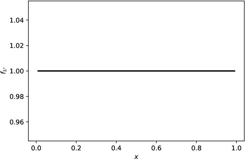
(a) The function $f_{\mathcal{U}}$.

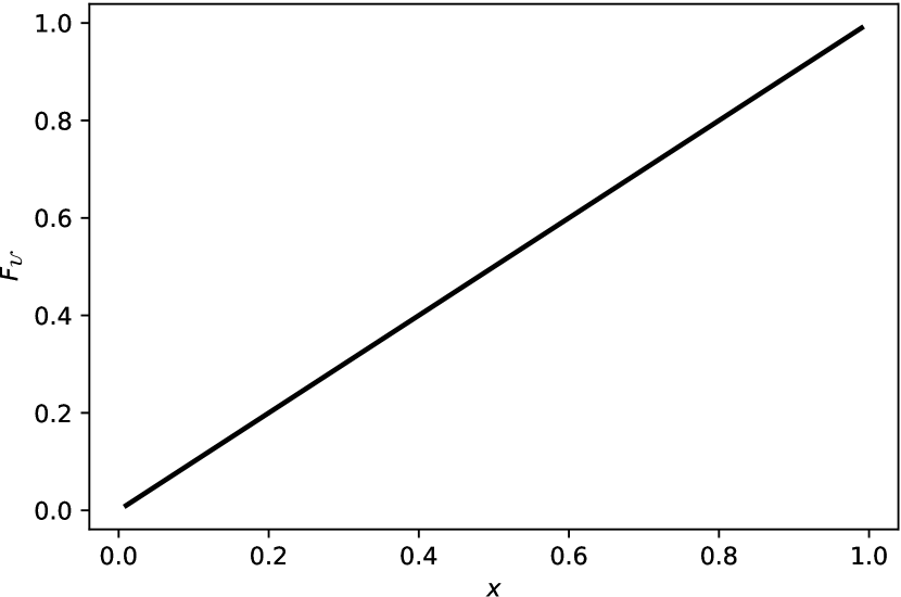
(b) The function $F_{\mathcal{U}}$.

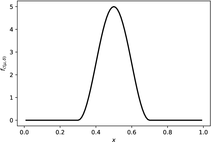
(c) The function $f_{\mathcal{C}(\mu,\delta)}$.

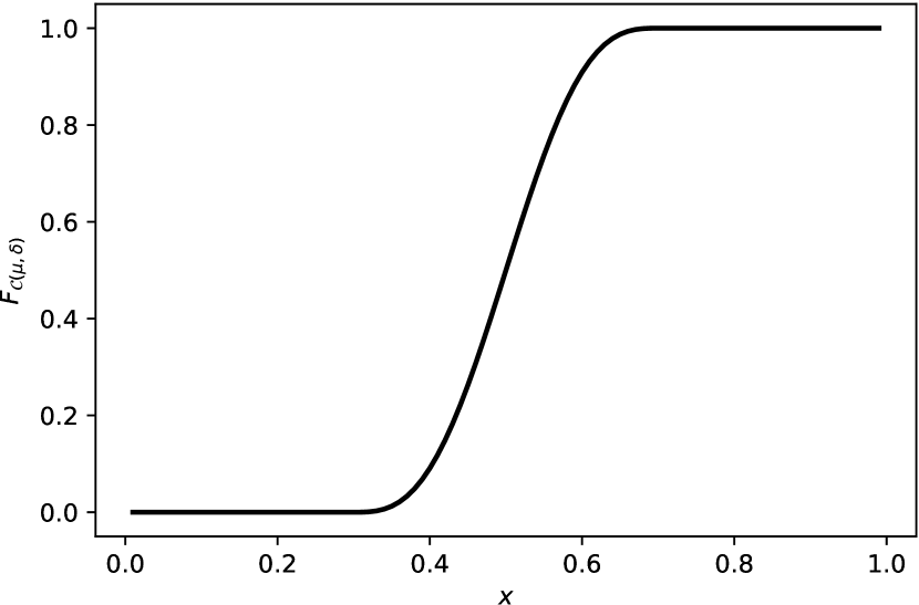
(d) The function $F_{\mathcal{C}(\mu,\delta)}$.

Figure 1: Top row: The functions $f_{\mathcal{U}}(x)$ (left panel) and $F_{\mathcal{U}}(x)$ (right panel), $x\in(0,1)$ for the uniform distribution. Bottom row: the functions $f_{\mathcal{C}(\mu,\delta)}(x)$ (left panel) and $F_{\mathcal{C}(\mu,\delta)}(x)$ (right panel), $x\in(0,1)$, for $\mu=0.5$ and $\delta=0.2$, for the raised cosine distribution.

We now test the performances of SOL functions relying on these two distribution functions, when applied to two actual binary classification problems.

A Python implementation of the SOLs is available for the scientific community at $\texttt{https://github.com/cesc14/SOL}\>.$

3.1 Optimized a posteriori thresholds and a priori distributions

We first considered the Adult training dataset [Kohavi96], where the task is to predict whether a person can make more than 50,000 dollars per year based on census data. First, we performed the following pre-processing steps:

1. We removed the samples containing missing values.

2. We dropped the feature education, which is highly correlated to the feature education-num. Indeed, both features concern the education level of the people in the dataset.

3. The possible values in the native-country column, which reports the country of origin of the people in the data set, were restricted to $1$ in place of United-States and $0$ for all other countries.

4. All categorical features were one-hot encoded. Finally, all features were standardized.

The resulting elements were then described by $48$ numerical features. The data set consisted of 30162 samples, where 7508 people made more than 50,000 dollars per year, while 22654 did not. As for the network architecture, we used a fully-connected feed-forward NN with an input layer ($50$ ReLu neurons), two hidden layers ($20$ and $5$ ReLu neurons) and a sigmoid output unit. During the training phase, $1/3$ of training set was used as a validation set. We trained the network on $500$ epochs and we imposed an early stopping condition when no improvement in the validation loss was obtained after $30$ epochs.

The following experiments were devoted to show how the choice of the distribution of the threshold $\tau$ affected the result of the a posteriori score maximization performed by varying the threshold in $(0,1)$. In doing so, we considered the SOL related to the f${}_{1}$-score [lipton2014optimal], which is the harmonic mean of precision and recall, i.e.

$$\textrm{f${}_{1}$-score}=\frac{2\textrm{TP}}{2\textrm{TP}+\textrm{FP}+\textrm{FN}}.$$

We observe that this score does not satisfy the linearity assumption in Theorem 2.7 (see also Remark 2.9).

We tested the uniform distribution $\mathcal{U}$ as well as the raised cosine distribution $\mathcal{C}(\mu,\delta)$ with different values of the parameters $\mu,\delta$. More precisely, for each combination of $(\mu,\delta)\in\{0.3,0.5,0.7\}\times\{0.1,0.2,0.3\}$ we randomly selected $4/5$ elements in the data set for training the NN and we performed the a posteriori score maximization on the training set. We repeated this procedure $100$ times.

In Table 1, we present the obtained results. We report that in some cases the training optimization process was unsuccessful, that is the validation loss got stuck from the beginning of the training, and no actual learning took place. Therefore, we did not include such cases in the computation of the other entries of the table.

Let $\eta\in\mathbb{N}$, $\eta\leq 100$, be the number of successful training processes. Figure LABEL:fig:adult compares the probability distribution chosen a priori for the threshold as in the left panel of Figure 1 (dashed blue line) to the empirical probability distribution $f_{\tau^{\star}}$ (red histograms) derived from the optimal thresholds $\tau^{\star}_{1},\dots,\tau^{\star}_{\eta}$ over the $\eta$ successful runs. We modelled this distribution via normalized histograms. Moreover, we also displayed the average optimal threshold (red cross) resulting from the $\eta$ runs. The horizontal solid red line indicates the standard deviation related to the optimal thresholds. These experiments show that the optimal threshold is indeed heavily influenced by the chosen distribution, which effectively drives the optimization process to prefer a certain interval of threshold values.

	Uniform	Raised cosine
		$\mu=0.3$		$\mu=0.5$		$\mu=0.7$
		$\delta=0.1$	$\delta=0.3$	$\delta=0.1$	$\delta=0.3$	$\delta=0.1$	$\delta=0.3$
#success	$100$	$90$	$100$	$100$	$100$	$83$	$100$
#out-of-support	$0$	$8$	$13$	$14$	$9$	$13$	$13$
#epochs	$119.46_{(\pm 43.95)}$	$125.21_{(\pm 44.39)}$	$121.05_{(\pm 46.14)}$	$124.07_{(\pm 42.27)}$	$131.12_{(\pm 48.89)}$	$124.00_{(\pm 44.97)}$	$123.08_{(\pm 38.51)}$
$\tau^{\star}$	$0.53_{(\pm 0.36)}$	$0.31_{(\pm 0.06)}$	$0.35_{(\pm 0.22)}$	$0.50_{(\pm 0.07)}$	$0.52_{(\pm 0.19)}$	$0.70_{(\pm 0.08)}$	$0.66_{(\pm 0.20)}$
f${}_{1}$-score($\tau^{\star})$	$0.7510_{(\pm 0.01)}$	$0.7578_{(\pm 0.01)}$	$0.7556_{(\pm 0.01)}$	$0.7557_{(\pm 0.01)}$	$0.7571_{(\pm 0.01)}$	$0.7549_{(\pm 0.01)}$	$0.7546_{(\pm 0.01)}$

Table 1: Outcomes of the application of the SOL functions in the case of a neural network trained on the Adult database. The chosen SOL relies on the $f_{1}$-score and the threshold $\tau$ is drawn according to the uniform and raised cosine distributions.

$$\begin{array}{c}\\ \\ \end{array}$$

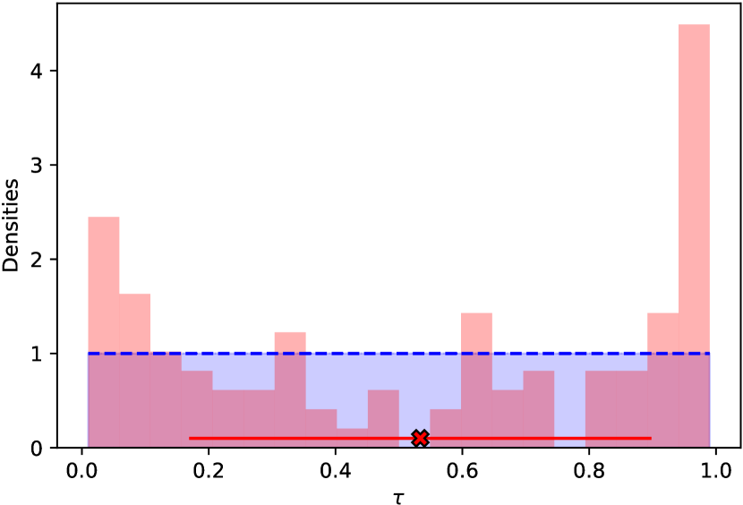
(a) Uniform

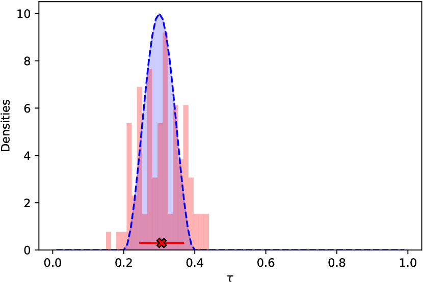
(b) Raisedcosine:μ=0.3,δ=0.1.

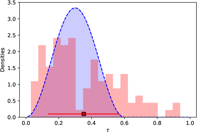
(c) Raisedcosine:μ=0.3,δ=0.3.