Online Flocking Control of UAVs with Mean-Field Approximation

Online Flocking Control of UAVs with Mean-Field Approximation

Abstract

This work presents a novel, inference-based approach to the distributed and cooperative flocking control of aerial robot swarms. The proposed method stems from the Unmanned Aerial Vehicle (UAV) dynamics by limiting the latent set to the robots’ feasible action space, thus preventing any unattainable control inputs from being produced and leading to smooth flocking behavior. By modeling the inter-agent relationships using a pairwise energy function, we show that interacting robot swarms constitute a Markov Random Field. Our algorithm builds on the Mean-Field Approximation and incorporates the collective behavioral rules: cohesion, separation, and velocity alignment. We follow a distributed control scheme and show that our method can control a swarm of UAVs to a formation and velocity consensus with real-time collision avoidance. We validate the proposed method with physical UAVs and high-fidelity simulation experiments.

I Introduction

With recent developments in aerial robotics, large-scale Unmanned Aerial Vehicle (UAV) swarms show potential in numerous application domains, such as environmental monitoring, performing search and rescue operations, and facilitating the burgeoning demand for mobile cellular networks [1, 2]. Extensive literature addresses the problem of controlling large gatherings of UAVs, with varying degrees of scalability, optimality, flight performance, and control architecture. However, as pointed out in recent work [3, 4, 5], coordinating such formations online while avoiding collisions is still challenging. Further, small-scale UAVs have limited computational capabilities, making it extremely difficult to perform computationally expensive controlling and planning on board.

These challenges have inspired researchers to investigate the functionality of biological swarms that richly demonstrate collective behavior while adhering to physical and dynamic constraints [6]. It has long been known that the flocking behavior of birds can be accounted for by a set of simple rules, namely cohesion, separation and velocity alignment [7] [8]. We propose a novel framework based on statistical inference to incorporate swarming rules to coordinate multiple robots. Specifically, our approach stems from the differentially flat dynamics of quadrotors and yields a formation and velocity consensus. Such a scheme bolsters the behavioral rules to the robots’ dynamics and thus significantly improves the feasibility of the trajectories by averting any unattainable control inputs. Since the outcome space follows the robots’ dynamic model, it greatly reduces the learning and tuning efforts needed.

Myriad literature from different domains, such as particle phase separation [9], image segmentation [10], and Simultaneous Localization And Mapping (SLAM) [11], amply explore Markov Random Field (MRF)-based approaches to model agent interactions in different systems. MRFs provide a compelling framework for describing the behavioral rules underlying flocking. Therefore, the key idea of this work subsumes the notion that a neighborhood of communicating robots in a swarm constitutes an MRF. By modeling the interactions among robots using a Self-Propelled Particle (SPP)-based energy function, we define a domain for the random variables induced by the robots’ control actions. We propose inference on the Markov network to approximate the best control input that minimizes the energy inside the neighborhood. Since our method’s coordination and collision avoidance depend on reacting to the neighborhoods online, we emphasize the necessity of a computationally tractable inference method. Thus, we propose using an approximate yet fast variational inference-based Mean-Field Approximation (MFA) to keep the computational effort bounded.

The main contribution of our work is a novel, distributed, flocking algorithm that combines differentially flat dynamics. We validate the consensus reaching procedure of our method with simulations and physical robot experiments. Further, we provide evaluation results for the convergence of the proposed algorithm for varying neighborhood sizes and a comparison of the velocity consensus reaching process against the Vicsek model [12]. In contrast to existing UAV swarm formation control methods [3] [5] [13], our method does not require explicit collision constraints or extensive training [2] [14]. Furthermore, due to the fast converging nature, our method is suitable for use in real-time aerial swarm coordination.

II Related Work

Numerous studies have been conducted on navigation and formation control of aerial robot swarms of varying sizes in indoor and outdoor environments [3, 5, 15, 16, 17]. Even though the state-of-the-art aerial swarms contain thousands of members, the trajectories are mainly precomputed and stored before execution [14]. Convex programming-based formation control methods are proposed in [4] [5] and [13] with online trajectory computations. However, none of the methods have demonstrated fundamental flocking behaviors, though [5] shows the capability to split and merge robot teams during the navigation. In [18], the authors used the collective motion of mosquitoes to derive a real-time pursuit law for quadrotors.

On the other hand, evolutionary algorithms [14] and graph neural network-based methods [2] have shown promise in achieving emergent behavior in quadrotor swarms with local communications. The authors have demonstrated flocking with cohesion and velocity consensus behaviors, yet the approaches are greatly susceptible to tuning and learning. Vásárhelyi et al. [19] reported unavoidable oscillations in the real hardware during the navigation incurred by the flocking controller. Further, [20] and [21] propose data-driven approaches for the vision-based flocking of quadrotors. In [22] and [23], the authors proposed an MRF-based approach to coordinate a swarm of robots. However, they discuss neither flocking consensus nor the dynamics of the particles.

Numerous methods have been proposed in the swarming community to simulate self-organizing behavior with propelled particle dynamics [24, 25, 26]. Many such methods suffer from issues of unbounded collision avoidance forces [26] and irregular fragmentation [6] [24]. These limitations, especially the former, can lead highly agile aerial vehicles to crash. Eliminating such unfeasible inputs while preserving the consensus is not trivial and highly dependent on tuning parameters. To address this issue, we tailor the control input space to suit the robots’ physical limitations by eliminating the possibility of producing dynamically unfeasible trajectories. We place our work in the conjuncture of aerial robot formation control, flocking algorithms, and multi-agent planning algorithms.

III Preliminaries

III-A Markov Random Fields

Markov networks or MRFs represent the relationships among interacting random variables when the directionality among them is irrelevant. In this work, we assume that there exist symmetrical interactions among homogeneous robots in a local neighborhood, and these constitute the framework of undirected graphical models. We start by defining the concept of factors in an MRF.

Let $X=\{X_{1},...,X_{N}\}$ be a set of random variables in an undirected graphical model.

Definition 1.

Let $D\subset X$. We define factor $\phi$ as a generic function that maps the values of $D$ to a real number. Thus, $\phi:\mathrm{Value}(D)\xrightarrow{}\mathbb{R}$.

We now define the joint probability distribution for $X$ parameterized by a set of factors $\Phi$.

Definition 2.

By considering a complete factorization $\Phi$ of distribution $X$, over subsets $D_{1},..,D_{M}$, we define the joint probability function as

$$P_{\Phi}(X_{1},...,X_{N})=\frac{1}{Z}\tilde{P}_{\Phi}(X_{1},...,X_{N}),$$ (1)

where $\tilde{P}_{\Phi}(X_{1},...,X_{N})=\phi_{1}(D_{1})\times\phi_{2}(D_{2})...\times\phi_{M}(D_{M})$ and $Z=\sum_{X_{1}...X_{N}}\tilde{P}_{\Phi}(X_{1},...,X_{N})$ is a normalizing constant called the partition function.

We now obtain a formulation where we can specify energies as factors. By using $\phi(D)=\exp{-\epsilon(D)}$, where $\epsilon$ is an energy function, and $\phi(D)>0$, we rewrite Eq. (1) as

$$P_{\Phi}(X)=P(X)=\frac{1}{Z}\exp{\{-\sum_{i}^{M}\epsilon_{i}(D_{i})\}}.$$ (2)

Eq. (2) is also known as the log-linear form of the Gibbs distribution, $P_{\Phi}(X_{1},...,X_{N})$, defined over the factorization $\Phi$. The strict positiveness of the factors ensures that the probability distribution is always positive. Further, we use this formulation to incorporate context-specific information of the UAV swarm in terms of energy functions. Particularly, Eq. (2) absorbs the concept that the interacting random variables prefer lower energy configurations, thus ideal for minimizing energies induced by other robots and the environment.

III-B Dynamic Model

We derive time parameterized trajectories defined for a differentially flat dynamic model of a quadrotor and a finite set of control actions. Similar to previous works on motion primitive-based planning [27], the state space of a robot consists of the position and its $(n-1)$-th derivatives. Let $x\in\mathbb{R}^{n\times 3}$ be the state space and $u\in\mathbb{R}^{3}$ be the control inputs of the dynamic system. We use the notation, $x=[p,\dot{p},...,p^{(n-1)}]^{T}$, and $u=p^{(n)}$ where $p\in\mathbb{R}^{3}$ is the position of the robot in $SE(3)$. By considering the differential flatness, we can represent the state space model as a linear time invariant dynamic system, $\dot{x}=Ax+Bu$ where,

$$A=\begin{bmatrix}0&I_{3}&0&\ldots&0\\ 0&0&I_{3}&\ldots&0\\ \vdots&\ddots&\ddots&\ddots&\vdots\\ 0&\ldots&\ldots&0&I_{3}\\ 0&\ldots&\ldots&0&0\end{bmatrix},B=\begin{bmatrix}0\\ 0\\ \vdots\\ 0\\ I_{3}\end{bmatrix}.$$ (3)

We show that given an initial state $x_{0}$ and a constant control input $u$, the trajectory of a linear time-invariant system can be represented by a time parameterized polynomial, which is differentiable at least $n$ times.

Assume time parameterized polynomial form for the resulting trajectory of the position $p(t)$,

$$p(t)=\sum_{q=0}^{\mathbf{q}}d_{q}\frac{t^{q}}{q!},$$

where $\mathbf{q}$ is the degree of the polynomial and $d_{q}$ is the $q$-th coefficient. As the control input is the $n$-th derivative of the position trajectory, by differentiating $n$ times,

$$u\equiv p^{(n)}(t)=\sum_{q=0}^{\mathbf{q}-n}d_{q+n}\frac{t^{q}}{q!}.$$

Considering $u$ is a constant control for the time interval, by analyzing the terms on the right hand side, we get the coefficients $d_{(n+1)}=d_{(n+2)}\dots d_{\mathbf{q}}=0$ and, $d_{n}=u$. By integrating this control expression $n$ times with the initial condition $x_{0}$,

$$p(t)=u\frac{t^{n}}{n!}+\dots+acc(x_{0})\frac{t^{2}}{2}+vel(x_{0})t+pos(x_{0}),$$ (4)

where $acc(x_{0})$, $vel(x_{0})$ and $pos(x_{0})$ denotes the acceleration, velocity and position components of the initial condition. As the degree of the position trajectory $p(t)$ is $n$, it is at least $n$ times differentiable in $t$ to obtain the higher-order states of the system such as velocity, acceleration, jerk, etc. Eq. (3) and Eq. (4) can be used to obtain the equivalent trajectory in state space form.

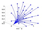
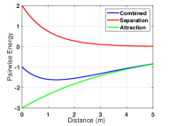
Figure 1: (a). Trajectories constructed for a robot with $vel(x_{0})=[1,0,1]^{T}$ and $pos(x_{0})=[0,0,0]^{T}$. (b) Morse potential energy function for $k_{r}=1$, $b=2$, $a=3$, $k_{a}=4$.

IV Approach

In this work, we consider a neighborhood for each robot in the swarm, following the topological swarming model proposed in [28]. We assume that the robots are capable of periodically obtaining the state of its neighbors, with a planning horizon $T_{H}$.

IV-A Robot Swarming Model

The number of neighbors in one’s interaction range directly affects the overall behavior of the swarm [29]; however, practical communication limitations hinder expanding the size of the neighborhood to the swarm width. The local neighborhood of any robot $i$ in our work consists of its $k$ nearest neighbors. We refer to $i$ as the root of the neighborhood. In addition to inter-agent relationships, we substantiate context-specific information to the swarming model in terms of external perturbations (e.g., obstacles, roost, and virtual boundaries). We discuss the quantification of such relationships within a swarm and represent them using energy functions. In order to represent different interactions within a swarm, we render two types of energy functions: pairwise (for robot-robot interactions) and unary (for external perturbations).

IV-A1 Interaction Energy

The interaction energy combines the cohesion and separation rules to define a pairwise energy function $\psi_{p}$ that has a minimum energy at a characteristic length-scale (Fig. 1[b]). Our formulation is similar to the Morse potential, which is a widely employed energy function in swarm and statistical physics domains [26] [30], to model the interactions among SPPs. For any two neighboring robots, $i$ and $j$, with states $x_{i}$ and $x_{j}$, we define $\psi_{p}$ as

$$\psi_{p}(x_{i},x_{j})=-a\exp{(-{\frac{\mathrm{d}_{ij}}{k_{a}}})}+b\exp{(-{\frac{\mathrm{d}_{ij}}{k_{r}}})},$$ (5)

where $\mathrm{d}_{ij}=\lVert pos(x_{i})-pos(x_{j})\rVert$, $k_{a},k_{r}>0$, $k_{a}>k_{r}$, $\frac{bk_{r}}{ak_{a}}<1$. We define the two terms in Eq. (5) as the attraction and the separation kernels, respectively. The defining characteristics of the Morse potential function depend on constraining the parameters $a$, $b$, $k_{a}$, and $k_{r}$ as mentioned. Fig. 1(b) shows the change of interaction energy with respect to the distance between two robots. Therefore, in the absence of external perturbations, we expect the robots to converge into a consensus formation with the average distance between the robots approximately equal to the local-minima of $\psi_{p}$.

IV-A2 Roosting Energy

We incorporate perturbations that solely depend on the state of an individual agent and sources that are external to the swarm as a unary energy function, $\psi_{u}$. The main purpose of the roosting energy function is to constrain the robots’ flocking to a geographical area of interest (roost). In real-world applications, one may design unary functions to represent an area with obstacles: a high-security zone in an urban environment, possibly demarcated by an equipotential line. Assuming that the only external perturbation in an obstacle-free environment is caused by their preference toward the roost, we define the roosting energy of a robot $i$ as a function of the position $pos(x_{i})$ and a roosting center $C_{R}\in\mathbb{R}^{3}$. Therefore,

$$\psi_{u}(x_{i})=\exp\{-{\frac{\lVert pos(x_{i})-C_{R}\rVert}{k_{R}}}\},$$ (6)

where $k_{R}>0$ and $C_{R}$ is a centroid of a known region in the environment, to which we refer as the roost.

IV-B Search Space

Planning motion in robots using a set of deterministic control actions is a well established concept and used in the literature [27] [31]. Typically, the discretized action space is combined with the robot’s state space using a state-action graph called state lattice, which is later coupled with a graph search to generate motion plans for robots. However, in multi-robot settings, the dimensionality of such state lattice representations tends to explode with the number of robots, possible actions, and states, making such methods computationally intractable in real time. Thus, we limit the search space in our work to a set of finite trajectories defined for a single planning horizon. By limiting the horizon length $T_{H}\to\delta t$, we achieve reactive and real-time behavior in robots. The cost of each trajectory is evaluated with respect to the energy functions ($\psi_{p}$ and $\psi_{u}$) and the state of each trajectory at the end of the planning horizon, $\delta t$ time.

First, we define a set of deterministic control actions based on the physical limitations of the robots. Let $u_{max}^{\textbf{d}}\in\mathbb{R}$ be the maximum possible control input for a robot over the axis d. Let $\textbf{d}_{u}$ be a discretization step. Hence, we define $\mu_{d}=(2u_{max}/\textbf{d}_{u}+1)$ number of control actions along dimension d, within $[-u_{max}^{\textbf{d}},u_{max}^{\textbf{d}}]$. By combining the control actions along the 3 dimensions, we obtain the control action space for any robot as $\mathcal{U}$ where the cardinality of $\mathcal{U}$ is $\mu_{X}\mu_{Y}\mu_{Z}$. Note that $\mathcal{U}$ is constant throughout the navigation. By exploiting the trajectory generation method presented in the preliminaries, we construct time-parameterized trajectories $l(t)$, for each control input $u\in\mathcal{U}$ and the robot state $x$. Without a loss of generalization, we extend the formulation in Eq. (4) to be a three-dimensional trajectory for any $u\in\mathbb{R}^{3}$ and $pos(x)\in\mathbb{R}^{3}$. For each $l(t)\in\mathbb{R}^{3}$ and $n=2$, where control inputs lie in the acceleration domain,

$$l(t)=u\frac{t^{2}}{2}+acc(x)\frac{t^{2}}{2}+vel(x)t+pos(x).$$ (7)

Therefore, for any robot $i$, we define a search space $\mathcal{L}_{i}$, such that $\mathcal{L}_{i}(\mathcal{U},x(t),t)=\{l_{i_{1}}(t),l_{i_{2}}(t),\dots\}$. Considering the differentially flat dynamics of aerial drones, we track any trajectory $l(t)$ along each dimension independently.

IV-C Markov Random Field Construction

Following the topological interaction rule, where each robot communicates with $k$ nearest neighbors, we construct a set of local neighborhoods. At the beginning of a planning horizon, each robot generates a complete (fully-connected) MRF corresponding to its local neighborhood. The completeness of the model helps us to embed the local information carried by each neighbor into the inference process. Formally, let $X=\{X_{1},X_{2},\dots\}$ be the random variables of MRF, where $X_{i}$ is associated with the $i$-th neighbor. Further, $Domain(X_{i})=\mathcal{L}_{i}(\mathcal{U},x_{i}(t),t)$. It is important to note that the graphical model and the domain of the random variables are instances of a time-varying spatial distribution as the robots move.

Let $G$ be the underlying graph of the MRF with a set of vertices $V$ and edges $\mathcal{E}$ where the the cardinality of $V$ is the number of robots in the local neighborhood.

Definition 3.

A clique $c$ of a graph $G$ is any complete subgraph of $G$.

Let $C$ be a clique factorization of $G$ that consists of singly, – $c_{u}$, and doubly, – $c_{p}$, connected cliques. Therefore, $c_{u},c_{p}\in C$. By associating previously defined pairwise and unary potential functions with each element in $C$, we define a Gibbs energy function for the local neighborhoods. Let $\Phi$ be the factorization of $X$ defined over $C$, where $\Phi_{p}$ and $\Phi_{u}$ are subsets of $\Phi$. For any $\phi_{u}\in\Phi_{u}$ and $\phi_{p}\in\Phi_{p}$, using the log linear form,

$$\phi_{u}(X_{i})=\exp{-\psi_{u}(x^{\prime}_{i})},$$ (8a)

$$\phi_{p}(X_{i},X_{j})=\exp{-\psi_{p}(x^{\prime}_{i},x^{\prime}_{j})},$$ (8b)

where $X_{i},X_{j}$ are two random variables in the MRF associated with robots $i,j$ and $x^{\prime}_{i}$ is the state of robot $i$ after a horizon length $\delta t$. Formally, $x^{\prime}_{i}=[l_{i}(t+\delta t),\dot{l}_{i}(t+\delta t),\ddot{l}_{i}(t+\delta t),\dots]^{T}$ for any $l_{i}\in\mathcal{L}_{i}$.

Theorem 1.

The probability of a local neighborhood forming in an environment can be parameterized by a set of pairwise and unary energy functions.

Proof.

Using the definition of Gibbs distribution in product form Eq. (1) for the MRF defined over a local neighborhood,

$$P_{\Phi}(X)\propto\prod_{\begin{subarray}{c}\phi_{u}\in\Phi_{u}\end{subarray}}\phi_{u}(c_{u})\prod_{\begin{subarray}{c}\phi_{p}\in\Phi_{p}\end{subarray}}\phi_{p}(c_{p}).$$ (9)

Substituting from the log linear form of factor potentials as in (8b),

$$P_{\Phi}(X)\propto\exp\{-\sum_{c_{u}}\psi_{u}(c_{u})-\sum_{c_{p}}\psi_{p}(c_{p})\}.$$ (10)

However, $c_{u}$ and $c_{p}$ are unary and pairwise cliques of $G$, and they consist of vertices and edges of the original graph. Since $G$ is fully connected, we write the above with associated random variables as

$$P_{\Phi}(X)\propto\exp\{-\sum_{i\leq N}\psi_{u}(x_{i})-\sum_{\begin{subarray}{c}i\leq N\\ j<i\end{subarray}}\psi_{p}(x_{i},x_{j})\}.$$ (11)

The summation of $\psi_{u}$ and $\psi_{p}$ inside the exponential function produces the neighborhood energy. It can be seen that the neighborhood energy changes with the value assigned to each random variable. Each trajectory assignment to the random variables postulates a different robotic formation at the end of the particular time horizon. As per the formulation of Eq.(11), higher neighborhood energies correspond to lower probabilities for the formation. Thus, we can use a Gibbs distribution parameterized by unary and pairwise factors to define the probability of each possible robot formation. ∎

Furthermore, any trajectory distribution over the MRF is analogous to the root robot’s predictions on the neighbors’ future actions given the local information.

IV-D Mean Field Approximation with Velocity Alignment

Given a fully connected MRF defined over a local neighborhood, we approximate the posterior distribution to obtain the best trajectory assignment that minimizes the neighborhood energy. As the search space and the neighborhood grow in size, the computational cost of exact inference methods increases by magnitudes and becomes intractable in real-time. Therefore, we propose using inexact yet fast MFA in this work. Further, we incorporate the velocity alignment property into the update rule as a compatibility function.

Briefly, we seek an approximate distribution $Q(X)=\prod_{i}Q_{i}(X_{i})$ that minimizes the Kullback-Leibler (KL) divergence with the true posterior distribution $P(X)$. One prevailing assumption in MFA is the independence of the random variables in the true posterior. However, as each planning horizon results in new posteriors, any disparities between the true and the approximated distributions will not be propagated into the future. By restricting the approximating posterior $Q(X)$ to a valid probability distribution and a product of the independent marginal distributions, we can obtain the following mean-field update rule. Due to the lengthy derivation of the update rule, we direct any interested readers to the Inference section of [32]. A disposition of the derivation can also be found in the supplementary material for [10].

$$D(Q||P_{\Phi})=\mathbb{E}_{\mathcal{U}\sim Q}[\ln\frac{Q(\mathcal{U})}{P_{\Phi}(\mathcal{U})}],$$

$$F(\tilde{P}_{\Phi},Q)=\sum_{\phi\in\Phi}\mathbb{E}_{Q}[\ln\phi]+\mathbb{H}_{Q}(\mathcal{U})$$

$$\mathrm{Find}\quad \{Q_{i}(\mathcal{U}_{i})\},$$

$$\mathrm{Maximizing}\quad F(\tilde{P}_{\Phi},Q)=\sum_{\phi\in\Phi}\mathbb{E}_{Q}[\ln\phi]+\mathbb{H}_{Q}(\mathcal{U}),$$

$$\mathrm{Subject\,to}\quad Q(\mathcal{U}_{i})=\prod_{i}{Q_{i}(\mathcal{U}_{i})},$$

$$\sum_{i}{Q_{i}(\mathcal{U}_{i})}=1.$$

$$Q_{i}(u_{i})=\frac{1}{Z_{i}}\exp\{-\psi_{u}(\dot{x}_{i})-\sum_{u_{j}\in\mathcal{U}_{j}}\mu(\dot{x}_{i},\dot{x}_{j})\sum_{j\neq i}\tilde{Q}_{j}(u_{j})\},$$

$$\tilde{Q}_{j}(u_{j})=Q_{j}(u_{j})\psi_{p}(\dot{x}_{i},\dot{x}_{j}).$$ (13)

In order to incorporate the velocity alignment behavioral rule, we define $\mu(x_{i}^{\prime},x_{j}^{\prime})$ as a velocity compatibility function that measures the distance between velocity components of $i$ and $j$ robots’ trajectory assignments. Therefore,

$$\mu(x_{i}^{\prime},x_{j}^{\prime})=\|vel(x_{i}^{\prime})-vel(x_{j}^{\prime}))\|.$$

Firstly, we calculate the expected pairwise energy of a trajectory assignment $l_{i}$ with respect to all the other robots $\sum_{j\neq i}\tilde{Q}_{j}(l_{j})$. Secondly, the velocity compatibility function penalizes the expected energy caused by the dissimilarity of the trajectories’ velocities. This increases the probability that the robots will have trajectories with likelier velocity components at the end of the time horizon. We consider the sum of the robots’ unary energy $\psi_{u}(x_{i}^{\prime})$ and the weighted, expected pairwise energy as the total Gibbs energy of a given trajectory $l_{i}$. Finally, we calculate the probability of each trajectory assignment $Q_{i}(l_{i})$ with Gibbs distribution Eq. (11).

Initialization

for $i\leftarrow 1\dots r\dots N$ do

       $\mathcal{L}_{i}\leftarrow\mathcal{L}_{i}(\mathcal{U},x_{i},t)$

       $Q_{i}(l_{i})\leftarrow\frac{1}{Z_{i}}\exp\{-\psi_{u}(\dot{x}_{i})\}$

      

end for

Approximation

while $Q_{old}(\mathcal{L})\neq Q(\mathcal{L})$ do

       $Q_{old}(\mathcal{L})\leftarrow Q(\mathcal{L})$

       $\tilde{Q}_{i}(l_{i})\leftarrow\sum_{j\neq i}Q_{j}(l_{j})\psi_{p}(\dot{x}_{i},\dot{x}_{j})$

       $\hat{Q}_{i}(l_{i})\leftarrow\sum_{l_{j}\in\mathcal{L}_{j}}\mu(\dot{x}_{i},\dot{x}_{j})\tilde{Q}_{i}(l_{i})$

       $Q_{i}(l_{i})\leftarrow\frac{1}{Z_{i}}\exp\{-\psi_{u}(\dot{x}_{i})-\hat{Q}_{i}(l_{i})\}$

      

end while

Execute $\operatorname*{arg\,max}_{l_{r}}Q_{r}(\mathcal{L}_{r})$ on robot $r$

Algorithm 1 Flocking algorithm for robot $r$

Algorithm 1 summarizes the key steps of our method into an iterative algorithm based on MFA. Here, we denote the root robot of the particular local neighborhood as $r$ and the size of the neighborhood as $N$. The algorithm runs on each robot $r$ in the swarm simultaneously. The initialization step computes the search space $\mathcal{L}_{i}$ for each robot in the neighborhood and their probability distributions based on the unary energies. We iterate the approximation step until the target probability distribution of each robot in the neighborhood converges. Finally, the root robot may execute the trajectory that maximizes the approximated marginal probability distribution of the corresponding RV.

V Experiments and Results

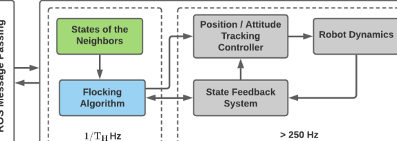
Figure 2: Overall design of the system. The components related to the robot dynamics and control (grey) runs over 250Hz. The flocking algorithm and the communication component run at a much slower rate.

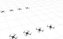
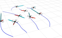
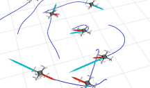
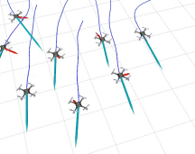
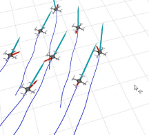
Figure 3: Snapshots of a swarm of drones at time (a) 0s, (b) 10s, (c) 20s, (d) 30s, (e) 40s, using $k=3$. For ease of visualization, the drones are controlled on a 2-dimensional plane of $20m\times 20m$. The blue lines show the trajectory trails of the robots for the last 5s. The red and cyan arrows depict the acceleration inputs and the current velocity of the robots, respectively. The lengths of the arrows are proportional to the size of the vectors in each dimension.

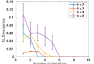
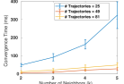
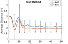
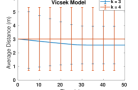
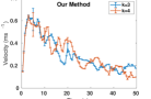
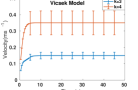
Figure 4: (a). Convergence rate of MFA. (b) Convergence time against the size of the search space and $k$. (c)(d) Average distance between the robots against the time. (e)(f) Average difference of velocities against time.

We experimented using the proposed method with teams of 3-10 quadrotors in physical and simulation environments. Each robot is armed with the tracking controller presented in [33], implemented on the Robot Operating System (ROS). For the hardware, we opted for Crazyflie 2.0 nano-drones with an external motion capture system for localization. For the experiments, we generated the trajectories with second-order ($n=2$) control inputs, according to Eq. (7). Fig. 2 visualizes the main components of our system and their connections. The flocking algorithm and the inter-vehicle communication modules run at a fixed rate of $1/T_{H}$ and the latter depends on the ROS communication layer. For physical experiments, we used radio communication to transfer the resulting control commands to the root robots. Typically, the internal controllers of the drones run at loop rates higher than $250Hz$ for attitude control; however, we executed the inter-vehicle communication and flocking algorithm modules at a much slower and more realistic $1/T_{H}=5Hz$ rate. To run the system with all the drone nodes and radio communications, we used a Linux system with an Intel $i7$ CPU and 16GB memory. Further, all the components were implemented in the C/C++ programming language. In addition, we used $u_{max}=1ms^{-2}$ and limited the maximum velocity of the robots to $1ms^{-1}$.

We assessed the convergence of the flocking algorithm for different search spaces with varying discretization steps, $\textbf{d}_{u}$. Fig. 3(a) shows the initial, stationary robot distribution used for the experiments. We modeled the pairwise potential function in Eq. (5) with $a=5,b=15,k_{a}=1.5,k_{r}=0.5$ and used the origin as the roosting center, $C_{R}$. We observed that changes in these parameters do not significantly affect the convergence rate of the flocking algorithm. However, changing the local minimum characteristics of the Morse potential reflects in the distances among the robots in the resulting cohesive aggregation.

Though individual robot controllers utilize incomplete information about the global state of the swarm, our algorithm achieved a formation and velocity consensus as in Figs. 3(d)-(e). Fig. 4(a) shows the convergence rate of the flocking algorithm against the neighborhood size. We used KL divergence to measure the distance between two adjacent target distributions ($Q_{old}(X),Q(X)$) in the approximation step. For a given planning horizon, the algorithm converged rapidly under 10 approximation iterations throughout the trials. Since the approximation step computes the expected pairwise energy of each trajectory for that of the neighbors, the computational cost grows quadratically with the neighborhood size. However, the proposed algorithm successfully converged within $200$ms for considerably large search spaces and $k$, which led the swarm to consensus 4(b). We experimented with a search space consisting of 25 trajectories and 10 robots and observed that the robots reached cohesion with minimal velocity differences while avoiding collisions with each other. Once converged, the shape of the formation remained roughly the same while maintaining the average distance among the robots as constant (Figs. 4(c), 5(a)).

We compared our method’s consensus reaching process to the algorithm proposed in [12], with the same topological and initial conditions. Briefly, self-propelled particles in the Vicsek model adjust their velocities and the heading directions in the neighborhood to reach the velocity consensus. Even though the Vicsek model reached the velocity consensus faster, Figs. 4(c)-(e) depict that the proposed method performed reasonably well to achieve even tighter alignments. Further, our method outperformed the Vicsek model by achieving cohesive formations, such as pentagons, by minimizing the interaction energy. In contrast, the particles in the Vicsek model did not show such behavior; refer to Fig. 4(d), as the original work overlooks the pairwise interactions [6]. We observed fragmentation in 3-dimensional formations caused by the highly combinatorial outcome space however, the motions visually resembled the collective behavior in natural swarms (Fig. 5(b)). Figs. 5(c)-(d) show the initial and final robots’ distributions for physical UAV experiments. We observed that collision avoidance to dependent on the parameters of the interaction energy, mainly when operating in tight indoor spaces. Although the interaction energy function in Eq.(5) considers a homogeneity assumption, we denote that the proposed framework is also extensible toward heterogeneous robot swarms with different attraction and repulsion kernels. Further, when coordinating swarms in outdoor environments, with large inter-robot distances, it is possible to increase the planning horizon to discount communication and perception delays while keeping the collective behavior intact. A supplementary video demonstration for this work can be found at: https://youtu.be/KVkNUKgViSg.

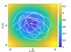
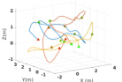
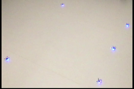
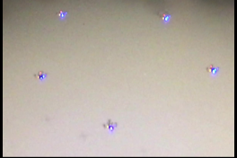
Figure 5: (a) Trajectories of the robots after reaching consensus, plotted over the roosting energy function. (b). Trajectories of 3 robots in 3D space. Colors of the robots’ markers change from green to red with time. (c) Initial and consensus reached formations (d) for five Crazyflie nano-drones.

VI Conclusions

In this work, we have proposed a novel approach to simulating flocking behavior with UAVs by utilizing the local information. We have employed an interaction energy-based approach to represent the robots’ relationships in the swarm. Our method embeds the UAV dynamics into the outcome-space and results in feasible trajectories for the vehicles. Consequently, our method eliminates the tedious parameter tuning phase of conventional flocking algorithms in practice. The resulting algorithm builds on MFA and can control a swarm of UAVs to flocking consensus while avoiding collisions. Due to the fast converging nature, this approach suits online UAV flocking control usage.

References

- [1] V. Sharma, M. Bennis, and R. Kumar, “Uav-assisted heterogeneous networks for capacity enhancement,” IEEE Communications Letters, vol. 20, no. 6, pp. 1207–1210, 2016.
- [2] E. Tolstaya, F. Gama, J. Paulos, G. Pappas, V. Kumar, and A. Ribeiro, “Learning decentralized controllers for robot swarms with graph neural networks,” in Conference on Robot Learning, pp. 671–682, 2020.
- [3] W. Hönig, J. A. Preiss, T. S. Kumar, G. S. Sukhatme, and N. Ayanian, “Trajectory planning for quadrotor swarms,” IEEE Transactions on Robotics, no. 99, pp. 1–14, 2018.
- [4] C. E. Luis, M. Vukosavljev, and A. P. Schoellig, “Online trajectory generation with distributed model predictive control for multi-robot motion planning,” IEEE Robotics and Automation Letters, vol. 5, no. 2, pp. 604–611, 2020.
- [5] H. Zhu, J. Juhl, L. Ferranti, and J. Alonso-Mora, “Distributed multi-robot formation splitting and merging in dynamic environments,” in 2019 International Conference on Robotics and Automation (ICRA), pp. 9080–9086, IEEE, 2019.
- [6] R. Olfati-Saber, “Flocking for multi-agent dynamic systems: Algorithms and theory,” IEEE Transactions on automatic control, vol. 51, no. 3, pp. 401–420, 2006.
- [7] C. W. Reynolds, “Flocks, herds and schools: A distributed behavioral model,” in ACM SIGGRAPH computer graphics, vol. 21, pp. 25–34, ACM, 1987.
- [8] A. Okubo, “Dynamical aspects of animal grouping: swarms, schools, flocks, and herds,” Advances in biophysics, vol. 22, pp. 1–94, 1986.
- [9] M. Blume, V. J. Emery, and R. B. Griffiths, “Ising model for the transition and phase separation in he 3-he 4 mixtures,” Physical review A, vol. 4, no. 3, p. 1071, 1971.
- [10] P. Krähenbühl and V. Koltun, “Efficient inference in fully connected crfs with gaussian edge potentials,” arXiv preprint arXiv:1210.5644, 2012.
- [11] K. S. Shankar and N. Michael, “Mrfmap: Online probabilistic 3d mapping using forward ray sensor models,” arXiv preprint arXiv:2006.03512, 2020.
- [12] T. Vicsek, A. Czirók, E. Ben-Jacob, I. Cohen, and O. Shochet, “Novel type of phase transition in a system of self-driven particles,” Physical review letters, vol. 75, no. 6, p. 1226, 1995.
- [13] J. Alonso-Mora, S. Baker, and D. Rus, “Multi-robot formation control and object transport in dynamic environments via constrained optimization,” The International Journal of Robotics Research, vol. 36, no. 9, pp. 1000–1021, 2017.
- [14] G. Vásárhelyi, C. Virágh, G. Somorjai, T. Nepusz, A. E. Eiben, and T. Vicsek, “Optimized flocking of autonomous drones in confined environments,” Science Robotics, vol. 3, no. 20, 2018.
- [15] M. Fernando and L. Liu, “Formation control and navigation of a quadrotor swarm,” in 2019 International Conference on Unmanned Aircraft Systems (ICUAS), pp. 284–291, IEEE, 2019.
- [16] M. Turpin, N. Michael, and V. Kumar, “Trajectory planning and assignment in multirobot systems,” in Algorithmic foundations of robotics X, pp. 175–190, Springer, 2013.
- [17] A. Weinstein, A. Cho, G. Loianno, and V. Kumar, “Visual inertial odometry swarm: An autonomous swarm of vision-based quadrotors,” IEEE Robotics and Automation Letters, vol. 3, no. 3, pp. 1801–1807, 2018.
- [18] D. Shishika and D. A. Paley, “Mosquito-inspired swarming for decentralized pursuit with autonomous vehicles,” in 2017 American Control Conference (ACC), pp. 923–929, IEEE, 2017.
- [19] G. Vásárhelyi, C. Virágh, G. Somorjai, N. Tarcai, T. Szörényi, T. Nepusz, and T. Vicsek, “Outdoor flocking and formation flight with autonomous aerial robots,” in 2014 IEEE/RSJ International Conference on Intelligent Robots and Systems, pp. 3866–3873, IEEE, 2014.
- [20] T.-K. Hu, F. Gama, Z. Wang, A. Ribeiro, and B. M. Sadler, “Vgai: A vision-based decentralized controller learning framework for robot swarms,” arXiv preprint arXiv:2002.02308, 2020.
- [21] F. Schilling, J. Lecoeur, F. Schiano, and D. Floreano, “Learning vision-based flight in drone swarms by imitation,” IEEE Robotics and Automation Letters, vol. 4, no. 4, pp. 4523–4530, 2019.
- [22] W. Xi, X. Tan, and J. S. Baras, “Gibbs sampler-based coordination of autonomous swarms,” Automatica, vol. 42, no. 7, pp. 1107–1119, 2006.
- [23] M. Fernando and L. Liu, “Swarming of aerial robots with markov random field optimization,” arXiv preprint arXiv:2010.06274, 2020.
- [24] H. G. Tanner, A. Jadbabaie, and G. J. Pappas, “Stable flocking of mobile agents part i: dynamic topology,” in 42nd IEEE International Conference on Decision and Control (IEEE Cat. No. 03CH37475), vol. 2, pp. 2016–2021, IEEE, 2003.
- [25] R. O. Saber and R. M. Murray, “Flocking with obstacle avoidance: Cooperation with limited communication in mobile networks,” in 42nd IEEE International Conference on Decision and Control (IEEE Cat. No. 03CH37475), vol. 2, pp. 2022–2028, IEEE, 2003.
- [26] V. Gazi, “On lagrangian dynamics based modeling of swarm behavior,” Physica D: Nonlinear Phenomena, vol. 260, pp. 159–175, 2013.
- [27] S. Liu, M. Watterson, K. Mohta, K. Sun, S. Bhattacharya, C. J. Taylor, and V. Kumar, “Planning dynamically feasible trajectories for quadrotors using safe flight corridors in 3-d complex environments,” IEEE Robotics and Automation Letters, vol. 2, no. 3, pp. 1688–1695, 2017.
- [28] M. Ballerini, N. Cabibbo, R. Candelier, A. Cavagna, E. Cisbani, I. Giardina, V. Lecomte, A. Orlandi, G. Parisi, A. Procaccini, et al., “Interaction ruling animal collective behavior depends on topological rather than metric distance: Evidence from a field study,” Proceedings of the national academy of sciences, vol. 105, no. 4, pp. 1232–1237, 2008.
- [29] Y. Shang and R. Bouffanais, “Influence of the number of topologically interacting neighbors on swarm dynamics,” Scientific reports, vol. 4, p. 4184, 2014.
- [30] J. A. Carrillo, S. Martin, and V. Panferov, “A new interaction potential for swarming models,” Physica D: Nonlinear Phenomena, vol. 260, pp. 112–126, 2013.
- [31] M. Pivtoraiko, R. A. Knepper, and A. Kelly, “Differentially constrained mobile robot motion planning in state lattices,” Journal of Field Robotics, vol. 26, no. 3, pp. 308–333, 2009.
- [32] D. Koller and N. Friedman, Probabilistic graphical models: principles and techniques. MIT press, 2009.
- [33] T. Lee, M. Leoky, and N. H. McClamroch, “Geometric tracking control of a quadrotor uav on se (3),” in Decision and Control (CDC), 2010 49th IEEE Conference on, pp. 5420–5425, IEEE, 2010.