Intelligent Reflecting Surfaces at Terahertz Bands: Channel Modeling and Analysis

Abstract

An intelligent reflecting surface (IRS) at terahertz (THz) bands is expected to have a massive number of reflecting elements to compensate for the severe propagation losses. However, as the IRS size grows, the conventional far-field assumption starts becoming invalid and the spherical wavefront of the radiated waves should be taken into account. In this work, we consider a spherical wave channel model and pursue a comprehensive study of IRS-aided multiple-input multiple-output (MIMO) in terms of power gain and energy efficiency (EE). Specifically, we first analyze the power gain under beamfocusing and beamforming, and show that the latter is suboptimal even for multiple meters away from the IRS. To this end, we derive an approximate, yet accurate, closed-form expression for the loss in the power gain under beamforming. Building on the derived model, we next show that an IRS can significantly improve the EE of MIMO when it operates in the radiating near-field and performs beamfocusing. Numerical results corroborate our analysis and provide novel insights into the design and performance of IRS-assisted THz communication.

I Introduction

Terahertz (THz) communication is widely deemed a key enabler for future 6G wireless networks due to the abundance of available spectrum at THz bands [1]. However, THz wireless links are subject to severe propagation losses, which require transceivers with a massive number of antennas to compensate for these losses and extend the communication range [2]. On the other hand, unlike sub-6 GHz systems, the power consumption of THz radio-frequency (RF) circuitry is considerably high, which might undermine the deployment of large antenna arrays in an energy efficient manner [3]. To overcome this problem, the novel concept of intelligent reflecting surface (IRS) can be exploited to build transceivers with a relatively small number of antennas, which work along with an IRS to achieve high spectral efficiency with reduced power consumption [4]. Thus, the performance analysis of IRS-aided THz communication is of great research importance.

There is a large body of literature investigating the modeling and performance of IRSs at sub-6 GHz and millimeter wave bands. Most of them, though, treat the IRS element as a typical antenna that re-radiates the impinging wave, and leverage antenna theory to characterize the path loss of the IRS-aided link. Furthermore, they assume far-field, where the spherical wavefront of the emitted waves degenerates to a plane wavefront. Although these approaches are popular due to their simplicity, they might not capture the unique features of IRSs, and especially at THz bands. To this direction, [5] introduced a path loss model for the sub-6 GHz band by invoking plate scattering theory, but assuming a specific scattering plane; hence, it is applicable only to special cases. The authors in [6] extended the said path loss model to arbitrary incident angles and polarizations, but considered the far-field zone of the IRS. Recently, a stream of papers (e.g., [7], [8], and references therein) proposed a path loss model that is applicable to near-field, using the “cos^q” radiation pattern [9] for each IRS element, which differs from the plate scattering-based model.

Although there are still many critical questions about the operation of THz IRSs, there is a dearth of related literature. From related work, we distinguish [10], where the authors showed that the far-field beampattern of a holographic IRS can be well approximated by that of an ultra-dense IRS, and then proposed a channel estimation scheme for THz massive multiple-input multiple-output (MIMO) aided by a holographic IRS. However, due to the high propagation losses and the short wavelength, a THz IRS is expected to consist of a massive number of passive reflecting elements, resulting in a radiating near-field, i.e., Fresnel zone, of several meters. Additionally, to effectively overcome the path loss of the transmitter-IRS link, the transmitter will need to operate near the IRS, which is in sharp contrast to sub-6 GHz massive MIMO of macrocell deployments. In conclusion, a THz IRS calls for a carefully tailored design that takes into account the aforementioned particularities.

This paper aims to shed light on these aspects, and study the channel modeling and performance of THz IRS. In particular:

• We provide a near-field channel model for THz frequencies. Our model is physically consistent, and takes into account the size of the IRS elements in the path loss calculation, as well as in the spherical wavefront of the radiated waves.

• We show that a typical THz IRS is likely to operate in the Fresnel zone, where conventional beamforming is suboptimal and hence can reduce the power gain. More importantly, we analytically evaluate that loss by providing an approximate closed-form expression.

• We compare IRS-aided MIMO with MIMO, and demonstrate the energy efficiency (EE) gains of the former architecture. More specifically, we determine the optimal number of IRS elements required to attain the same rate as MIMO with reduced power consumption, and reveal the EE scaling laws.

Notation: $D_{N}(x)=\frac{\sin(Nx/2)}{N\sin(x/2)}$ is the Dirichlet sinc function; $\mathbf{A}$ is a matrix; $\mathbf{a}$ is a vector; $[\mathbf{A}]_{i,j}$ is the $(i,j)$th entry of $\mathbf{A}$; $\mathbf{A}^{T}$ and $\mathbf{A}^{H}$ are the transpose and conjugate transpose of $\mathbf{A}$, respectively, $\text{vec}(\mathbf{A})$ is the column vector formed by stacking the columns of $\mathbf{A}$; and $\mathcal{CN}(\bm{\mu},\bm{\Sigma})$ is a complex Gaussian vector with mean $\bm{\mu}$ and covariance matrix $\bm{\Sigma}$.

Figure 1: Illustration of the IRS geometry considered in the channel model.

II System Model

II-A Signal Model

Consider a THz IRS system where the transmitter (Tx) and receiver (Rx) have a single antenna each. The IRS is placed in the $xy$-plane, and it consists of $N=N_{x}\times N_{y}$ passive reflecting elements. Each reflecting element is of size $L_{x}\times L_{y}$, and the spacings between adjacent elements are $\bar{d}_{x}$ and $\bar{d}_{y}$ along the $x$ and $y$ directions, respectively. The reflection coefficient of the $(n,m)$th IRS element is $e^{j\varphi_{n,m}}$, where $\varphi_{n,m}\in[-\pi,\pi]$. We next focus on the Tx-IRS-Rx link. The baseband signal at the receiver is then written as

$$y=\mathbf{h}^{T}_{r}\mathbf{\Phi}\mathbf{h}_{t}s+\tilde{n},$$ (1)

where $\mathbf{\Phi}=\text{diag}(\text{vec}(\tilde{\mathbf{\Phi}}))\in\mathbb{C}^{N\times N}$, with $\tilde{\mathbf{\Phi}}\in\mathbb{C}^{N_{x}\times N_{y}}$ and $[\tilde{\mathbf{\Phi}}]_{n,m}=e^{j\varphi_{n,m}}$, is the IRS’s reflection matrix, $\mathbf{h}_{r}\in\mathbb{C}^{N\times 1}$ is the channel from the Rx to the IRS, $\mathbf{h}_{t}\in\mathbb{C}^{N\times 1}$ is the channel from the Tx to the IRS, $s\sim\mathcal{CN}(0,P_{t})$ is the transmitted data symbol, $P_{t}$ is the average power per data symbol, and $\tilde{n}\sim\mathcal{CN}(0,\sigma^{2})$ is the additive noise.

II-B Channel Model

II-B1 Spherical Wavefront

Unlike antenna arrays that are typically modeled as a collection of point radiators, an IRS comprises rectangular reflecting elements whose size cannot be neglected. Assume that the center of the $(0,0)$th IRS element is placed at the origin of the coordinate system, as shown in Fig. 1. Across the $(n,m)$th IRS element, the reflection coefficient $e^{j\varphi_{n,m}}$ remains constant, and the phase difference between adjacent elements is measured from their centers. Thus, the position vector of the $(n,m)$th IRS element is $\mathbf{p}_{n,m}=\left(nd_{x},md_{y},0\right)$, where $d_{x}\triangleq\bar{d}_{x}+L_{x}$ and $d_{y}\triangleq\bar{d}_{y}+L_{y}$. Let $\lambda$ denote the carrier wavelength. Henceforth, we consider $L_{x}=L_{y}=\lambda/2$ and $\bar{d}_{x}=\bar{d}_{y}=0$ [8, 11].

The Tx and Rx are located in $(D_{t},\theta_{t},\phi_{t})$ and $(D_{r},\theta_{r},\phi_{r})$, respectively, and hence their position vectors in Cartesian coordinates are

$$\mathbf{p}_{t} =(D_{t}\cos\phi_{t}\sin\theta_{t},D_{t}\sin\phi_{t}\sin\theta_{t},D_{t}\cos\theta_{t}),$$ (2)

$$\mathbf{p}_{r} =(D_{r}\cos\phi_{r}\sin\theta_{r},D_{r}\sin\phi_{r}\sin\theta_{r},D_{r}\cos\theta_{r}),$$ (3)

where $D_{t}$ and $D_{r}$ are the distances measured from the (0,0)th IRS element, while $\phi$ and $\theta$ denote the azimuth and polar angles, respectively. The baseband channel from the Tx to the IRS is specified as $\mathbf{h}_{t}=\text{vec}(\mathbf{M}_{t})$, where $\mathbf{M}_{t}\in\mathbb{C}^{N_{x}\times N_{y}}$ is the auxiliary matrix with entries [12]

$$[\mathbf{M}_{t}]_{n,m}=\sqrt{\text{PL}^{t}_{n,m}}e^{-jkD^{t}_{n,m}}.$$ (4)

In (4), $k=\frac{2\pi}{\lambda}$ is the wavenumber, $\text{PL}^{t}_{n,m}$ is the path loss between the Tx and the $(n,m)$th IRS element, and $D^{t}_{n,m}\triangleq\|\mathbf{p}_{t}-\mathbf{p}_{n,m}\|$ is the respective distance, with $D^{t}_{0,0}=D_{t}$. Similarly, we have $\mathbf{h}_{r}=\text{vec}(\mathbf{M}_{r})$, where $\mathbf{M}_{r}\in\mathbb{C}^{N_{x}\times N_{y}}$ is the auxiliary matrix with entries

$$[\mathbf{M}_{r}]_{n,m}=\sqrt{\text{PL}^{r}_{n,m}}e^{-jkD^{r}_{n,m}},$$ (5)

where $\text{PL}^{r}_{n,m}$ is the path loss between the Rx and the $(n,m)$th IRS element, and $D^{r}_{n,m}\triangleq\|\mathbf{p}_{r}-\mathbf{p}_{n,m}\|$, with $D^{r}_{0,0}=D_{r}$. Using (4) and (5), the received signal in (1) is recast as

$$y=\sum_{n=0}^{N_{x}-1}\sum_{m=0}^{N_{y}-1}\sqrt{\text{PL}_{n,m}}e^{-jk(D^{t}_{n,m}+D^{r}_{n,m})}e^{j\varphi_{n,m}}s+\tilde{n},$$ (6)

where $\text{PL}_{n,m}=\text{PL}^{t}_{n,m}\text{PL}^{r}_{n,m}$ denotes the overall path loss of the Tx-IRS-Rx link through the $(n,m)$th reflecting element. Hence, the receive signal-to-noise ratio (SNR) is

$$\text{SNR}=\frac{P_{t}}{\sigma^{2}}\left|\sum_{n=0}^{N_{x}-1}\sum_{m=0}^{N_{y}-1}\sqrt{\text{PL}_{n,m}}e^{-jk(D^{t}_{n,m}+D^{r}_{n,m})}e^{j\varphi_{n,m}}\right|^{2}.$$ (7)

In the sequel, we detail the path loss model for THz bands, which relies on the plate scattering paradigm [13].

II-B2 Scattered Field by an IRS Element

We focus on an arbitrary IRS element and omit the subscript “$n,m$” hereafter. The Tx and Rx are in the far-field of the individual element, which implies that $D_{t},D_{r}>2L^{2}_{\max}/\lambda$, where $2L^{2}_{\max}/\lambda$ is the Fraunhofer distance and $L_{\max}=\max(L_{x},L_{y})$ is the maximum dimension of the element. Consequently, a plane wavefront is assumed across the IRS element. For simplicity, we consider a transverse electric incident wave which is linearly polarized along the $x$-axis. The electric field (E-field) of the incident plane wave is hence given by

$$\mathbf{E}_{i} =E_{i}e^{-jk(y\sin\theta_{t}-z\cos\theta_{t})}\mathbf{e}_{x},$$ (8)

where $\mathbf{e}_{x}$ denotes the unit vector along the $x$-axis. Next, the scattered field $\mathbf{E}_{s}$ at the receiver location $(D_{r},\theta_{r},\phi_{r})$ is determined using physical optics techniques, whereby the IRS element is modeled as a perfectly conducting plate. Specifically, the squared magnitude of the scattered E-field is given by [13, Ch. 11]

$$\|\mathbf{E}_{s}\|^{2} =\left(\frac{L_{x}L_{y}}{\lambda}\right)^{2}\frac{|E_{i}|^{2}}{D^{2}_{r}}F(\theta_{t},\phi_{r},\theta_{r})\text{sinc}^{2}(X)\text{sinc}^{2}(Y)$$ (9)

$$\approx\left(\frac{L_{x}L_{y}}{\lambda}\right)^{2}\frac{|E_{i}|^{2}}{D^{2}_{r}}F(\theta_{t},\phi_{r},\theta_{r}),$$ (10)

where $F(\theta_{t},\phi_{r},\theta_{r})\triangleq\cos^{2}\theta_{t}(\cos^{2}\theta_{r}\cos^{2}\phi_{r}+\sin^{2}\phi_{r})$, while $X\triangleq\frac{\pi L_{x}}{\lambda}\sin\theta_{r}\cos\phi_{r}$ and $Y\triangleq\frac{\pi L_{y}}{\lambda}(\sin\theta_{r}\sin\phi_{r}-\sin\theta_{t})$.

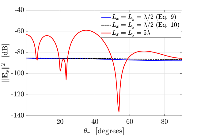
Figure 2: Squared magnitude of the scattered field versus observation angle $\theta_{r}$ for incident angle $\theta_{t}=30\degree$ and scattering plane $\phi_{r}=60\degree$; $|E_{i}|^{2}=1$, carrier frequency $f=300$ GHz, and $D_{r}=4$ meters.

The approximation in (10) follows from $\text{sinc}(X)\approx 1$ and $\text{sinc}(Y)\approx 1$ for $X\approx 0$ and $Y\approx 0$, which holds for $L_{x}\leq\lambda$ and $L_{y}\leq\lambda$. This is also verified in Fig. 2. It is worth stressing that each IRS element is expected to be of sub-wavelength size in order to act as an isotropic scatterer [14].

II-B3 Path Loss

Recall that the relation between $P_{t}$ and $E_{i}$ is $|E_{i}|^{2}/(2\eta)=P_{t}G_{t}/(4\pi D^{2}_{t})$, where $\eta$ is the free-space impedance, and $G_{t}$ is the transmit antenna gain [15]. Hence, the power density of the scattered field is

$$S_{s}=\frac{\|\mathbf{E}_{s}\|^{2}}{2\eta}=\left(\frac{L_{x}L_{y}}{\lambda}\right)^{2}\frac{P_{t}G_{t}}{4\pi D_{t}^{2}D^{2}_{r}}F(\theta_{t},\phi_{r},\theta_{r}).$$ (11)

Considering the receive aperture $A_{r}=G_{r}\lambda^{2}/(4\pi)$ yields the receive power

$$P_{r}=S_{s}A_{r}=P_{t}\frac{G_{t}G_{r}}{(4\pi D_{t}D_{r})^{2}}(L_{x}L_{y})^{2}F(\theta_{t},\phi_{r},\theta_{r}).$$ (12)

Finally, taking into account the molecular absorption losses at THz bands gives the path loss of the Tx-IRS-Rx link through the $(n,m)$th element

$$\text{PL}_{n,m}=\frac{G_{t}G_{r}(L_{x}L_{y})^{2}}{(4\pi D^{t}_{n,m}D^{r}_{n,m})^{2}}F(\theta_{t},\phi_{r},\theta_{r})e^{-\kappa_{\text{abs}}(f)(D^{t}_{n,m}+D^{r}_{n,m})},$$ (13)

where $\kappa_{\text{abs}}(f)$ is the molecular absorption coefficient at the carrier frequency $f$. From Fig. 3, we see that $\text{PL}_{n,m}$ marginally changes across the IRS, even for $100\times 100$ elements and a Tx distance $D_{t}=0.67$ m. This is because of the small physical size of the IRS at THz bands. Hereafter, we will assume that $\text{PL}_{n,m}\approx\text{PL}$, where PL is calculated using $D_{t}$ and $D_{r}$ measured from the $(0,0)$th IRS element.

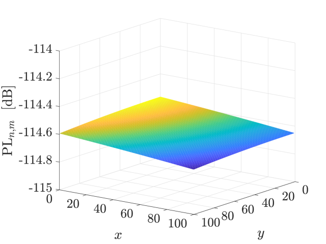
Figure 3: Path loss across an $100\times 100$-element IRS; $f=300$ GHz, $\kappa_{\text{abs}}(f)=0.0033$ m^-1, $L_{x}=L_{y}=\lambda/2$, $\bar{d}_{x}=\bar{d}_{y}=0$, $G_{t}=G_{r}=20$ dBi, $\mathbf{p}_{t}=(0,-0.3,0.6)$, $D_{t}=0.67$ m, $\mathbf{p}_{r}=(0,1,1)$, and $D_{r}=1.41$ m.

TABLE I: IRS with $L_{x}=L_{y}=\lambda/2$ and $\bar{d}_{x}=\bar{d}_{y}=0$ at $f=300$ GHz.

$N_{x}\times N_{y}$-elements	Physical Size [$\text{m}^{2}$]	Fresnel Region [m]
$80\times 80$	$0.039\times 0.039$	$[0.15,3.2]$
$100\times 100$	$0.05\times 0.05$	$[0.22,5]$

III Power Gain of IRS-Aided THz System

III-A Fresnel Region

The near-field of an IRS refers to distances that are smaller than the Fraunhofer distance $D_{F}\triangleq 2L^{2}_{\text{IRS}}/\lambda$, where $L_{\text{IRS}}\triangleq\max\left(N_{x}L_{x}+(N_{x}-1)\bar{d}_{x},N_{y}L_{y}+(N_{y}-1)\bar{d}_{y}\right)$ is the maximum physical dimension of the IRS. In our work, we focus on the radiating near-field, i.e., Fresnel region, which corresponds to distances $D\gg\lambda$ satisfying [15]

$$0.62\sqrt{L^{3}_{\text{IRS}}/\lambda}<D\leq 2L^{2}_{\text{IRS}}/\lambda.$$ (14)

From Table I, we verify the small physical size of THz IRS, as well as its large Fresnel region. Consequently, it is very likely that the Tx and Rx are in the near-field of the IRS, where the spherical wavefront of the impinging waves across the IRS cannot be neglected.

III-B Near-Field Beamfocusing

Let us define the normalized power gain as

$$G\triangleq\frac{\left|\sum_{n=0}^{N_{x}-1}\sum_{m=0}^{N_{y}-1}e^{-jk\left(D^{t}_{n,m}+D^{r}_{n,m}\right)}e^{j\varphi_{n,m}}\right|^{2}}{N_{x}^{2}N_{y}^{2}},$$ (15)

with $G\in[0,1]$. The receive SNR in (7) is now written as

$$\text{SNR}\approx\frac{N^{2}GP_{t}\text{PL}}{\sigma^{2}}.$$ (16)

The power gain is maximized by near-field beamfocusing. Hence, the phase induced by the $(n,m)$th IRS element is

$$\varphi_{n,m}=k\left(D^{t}_{n,m}+D^{r}_{n,m}\right),$$ (17)

which yields $G=1$ and $\text{SNR}=N^{2}P_{t}\text{PL}/\sigma^{2}$. As expected, the SNR of an IRS-aided system grows quadratically with the number $N$ of IRS elements [16]. Note, though, that the IRS needs to know the exact locations of the Tx and Rx in order to perform beamfocusing.

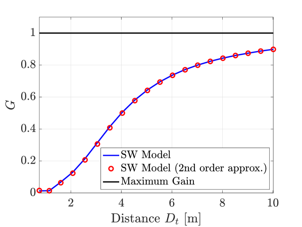
(a)

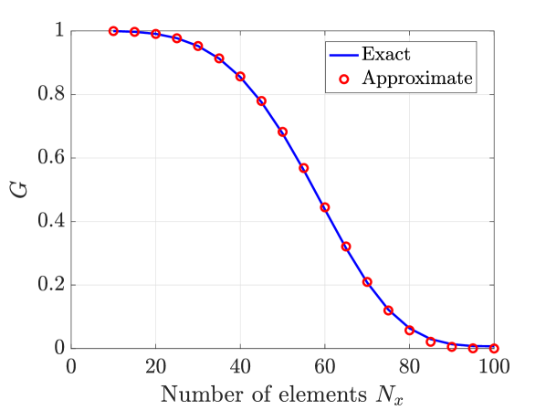
(b)

Figure 4: (a) Normalized power gain vs. distance $D_{t}$ for an $100\times 100$-element IRS, where $\mathbf{p}_{t}=(0.4,0.4,z)$, $0.5\leq z\leq 10$, and $0.755\leq D_{t}\leq 10.016$ m. (b) Normalized power gain vs. number of elements for an $N_{x}\times N_{y}$-element IRS, where $N_{x}=N_{y}$, $\mathbf{p}_{t}=(0.4,0.4,1)$, and $D_{t}=1.15$ m. The other parameters are $f=300$ GHz, $L_{x}=L_{y}=\lambda/2$, and $\bar{d}_{x}=\bar{d}_{y}=0$.

III-C Far-Field Beamforming

In this section, we analyze the power gain under conventional far-field beamforming, which relies on the parallel ray approximation. First, using basic algebra, we have that

$$D^{r}_{n,m}= D_{r}\left(1+\frac{(nd_{x})^{2}}{D_{r}^{2}}-\frac{2\cos\phi_{r}\sin\theta_{r}nd_{x}}{D_{r}}\right.$$

$$\quad\quad\quad\left.+\frac{(md_{y})^{2}}{D_{r}^{2}}-\frac{2\sin\phi_{r}\sin\theta_{r}md_{y}}{D_{r}}\right)^{1/2}.$$ (18)

In the far-field $D_{r}\gg D_{F}$, the first-order Taylor expansion $(1+x)^{a}\approx 1+ax$ can be applied to (III-C), while ignoring the quadratic terms $(nd_{x})^{2}/D_{r}^{2}$ and $(md_{y})^{2}/D_{r}^{2}$. This yields

$$D^{r}_{n,m}\approx D_{r}-nd_{x}\cos\phi_{r}\sin\theta_{r}-md_{y}\sin\phi_{r}\sin\theta_{r},$$ (19)

which corresponds to the plane wavefront model.

Remark 1.

The far-field steering vector is defined as $\mathbf{a}(\phi,\theta)\triangleq\emph{vec}(\mathbf{M})$, where $\mathbf{M}\in\mathbb{C}^{N_{x}\times N_{y}}$ is the matrix with elements $[\mathbf{M}]_{n,m}=e^{jk(nd_{x}\cos\phi\sin\theta+md_{y}\sin\phi\sin\theta)}$. Thus, the channel vector is $\mathbf{h}=\sqrt{\emph{PL}}e^{-jkD}\mathbf{a}(\phi,\theta)$.

Let us now consider that the Rx is in the far-field of the IRS whilst the Tx is close to the IRS; in fact, this deployment yields the maximum SNR, compared to placing the IRS somewhere in between [17]. If the IRS employs beamforming based on the angular information $(\phi_{t},\theta_{t})$ and $(\phi_{r},\theta_{r})$, i.e.,

$$\varphi_{n,m}=-k( nd_{x}\cos\phi_{t}\sin\theta_{t}+md_{y}\sin\phi_{t}\sin\theta_{t}$$

$$+nd_{x}\cos\phi_{r}\sin\theta_{r}+md_{y}\sin\phi_{r}\sin\theta_{r}),$$ (20)

the power gain will decrease. To analytically characterize this reduction, we use the second-order Taylor expansion $(1+x)^{a}\approx 1+ax+\frac{1}{2}a(a-1)x^{2}$ and neglect the terms $O(d^{q}/D^{q}),q\geq~{}3$, which yields the (Fresnel) approximation of the Tx distance

$$D^{t}_{n,m}\approx D_{t} +\frac{(nd_{x})^{2}(1-\cos^{2}\phi_{t}\sin^{2}\theta_{t})}{2D_{t}}-nd_{x}\cos\phi_{t}\sin\theta_{t}$$

$$+\frac{(md_{y})^{2}(1-\sin^{2}\phi_{t}\sin^{2}\theta_{t})}{2D_{t}}-md_{y}\sin\phi_{t}\sin\theta_{t}.$$ (21)

Using (19), (III-C) and (III-C), the normalized power gain in (15) reduces to the expession (V-B) at the top of the last page. The accuracy of the approximation of the Tx distance is depicted in Fig. 4(4(a)), and the validity of (V-B) is evaluated in Fig. 4(4(b)). Note that the lower limit of the Fresnel zone of an $100\times 100$-element IRS, with $L_{x}=L_{y}=\lambda/2$ and $\bar{d}_{x}=\bar{d}_{y}=0$, is $0.22$ meters according to Table I. Thus, the distances in the numerical experiments were chosen so that the Tx does not operate in the reactive near-field. As observed, beamforming can substantially decrease the power gain even for distances of several meters away from the IRS. This is because of the mismatch between (17) and (III-C). Moreover, from (V-B), we have the asymptotic result $G\to 0$ as $N\to\infty$. In conclusion, near-field beamfocusing should be used in most cases of interest.

IV Performance of IRS-Aided THz System

IV-A Benchmark: MIMO System

Consider a MIMO system, where the Tx and Rx are equipped with $N_{t}$ and $N_{r}$ antennas, respectively. For efficient hardware implementation, hybrid array architectures are assumed at both ends. The path loss of the direct channel, i.e., line-of-sight (LoS), is given by

$$\text{PL}_{\text{MIMO}}=\frac{G_{t}G_{r}\lambda^{2}}{(4\pi D_{d})^{2}}e^{-\kappa_{\text{abs}}(f)D_{d}},$$ (23)

where $D_{d}=\|\mathbf{p}_{r}-\mathbf{p}_{t}\|$. Assuming far-field, the LoS channel is rank-one. Then, analog beamforming and combining yield the receive SNR

$$\text{SNR}_{\text{MIMO}}=\frac{N_{r}N_{t}P_{t}\text{PL}_{\text{MIMO}}}{\sigma^{2}}.$$ (24)

Lastly, the respective power consumption is calculated as

$$P^{\text{MIMO}}_{c}=P_{t}+N_{r}(P_{\text{PS}}+P_{\text{PA}})+N_{t}(P_{\text{PS}}+P_{\text{PA}}),$$ (25)

where $P_{\text{PS}}=42$ mW and $P_{\text{PA}}=60$ mW are the power consumption values for a phase shifter and a power amplifier at $f=300$ GHz, respectively [3].

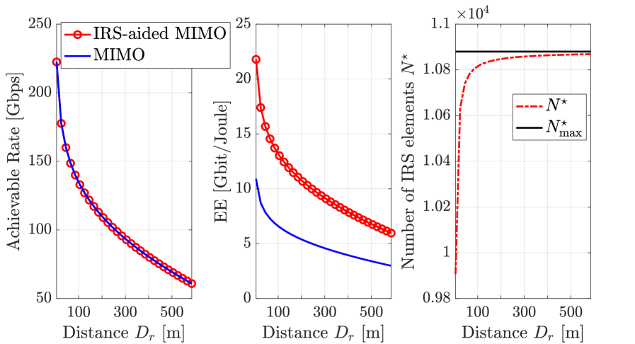
Figure 5: Achievable rate, EE, and number of IRS elements versus distance $D_{r}$ for $\alpha=2$ and a fixed IRS location at (0,0,0). In the MIMO system, $N_{t}=100$ and $N_{r}=100$. The other parameters are $G_{t}=G_{r}=20$ dBi, $P_{t}=10$ dBm, $\sigma^{2}=-174$ dBm/Hz, $B=10$ GHz, $f=300$ GHz, $L_{x}=L_{y}=\lambda/2$, $\mathbf{p}_{t}=(0,-0.6,1)$ with $D_{t}=1.16$ m, and $\mathbf{p}_{r}=(0,D_{r},1)$.

IV-B IRS-Assisted MIMO System

The Tx and Rx perform beamforming and combining to communicate a single stream through an IRS of $N$ elements. Due to the directional transmissions, the Tx-Rx link is negligible, and thus is ignored. The received signal through the Tx-IRS-Rx channel is given by

$$y=\mathbf{w}^{H}(\mathbf{H}_{r}\mathbf{\Phi}\mathbf{H}_{t}\mathbf{f}s+\tilde{\mathbf{n}}),$$ (26)

where $\mathbf{w}\in\mathbb{C}^{N_{r}\times 1}$ is the combiner, $\mathbf{f}\in\mathbb{C}^{N_{t}\times 1}$ is the beamformer, $\mathbf{H}_{t}\in\mathbb{C}^{N\times N_{t}}$ is the channel from the Tx to the IRS, $\mathbf{H}_{r}\in\mathbb{C}^{N_{r}\times N}$ is the channel from the IRS to the Rx, and $\tilde{\mathbf{n}}\sim\mathcal{CN}(\mathbf{0},\sigma^{2}\mathbf{I}_{N_{r}})$ is the noise vector. For ease of exposition, we assume far-field for both the Tx and the Rx. Then,

$$\mathbf{H}_{r} =\sqrt{\text{PL}_{r}}e^{-jkD_{r}}\mathbf{a}_{r}(\phi_{\text{rx}},\theta_{\text{rx}})\mathbf{a}^{H}_{\text{IRS}}(\phi_{r},\theta_{r}),$$ (27)

$$\mathbf{H}_{t} =\sqrt{\text{PL}_{t}}e^{-jkD_{t}}\mathbf{a}_{\text{IRS}}(\phi_{t},\theta_{t})\mathbf{a}^{H}_{t}(\phi_{\text{tx}},\theta_{\text{tx}}),$$ (28)

where $\text{PL}_{t}\approx\text{PL}^{t}_{n,m}$ and $\text{PL}_{r}\approx\text{PL}^{r}_{n,m}$; the far-field response vectors $\mathbf{a}_{r}(\cdot,\cdot)$, $\mathbf{a}_{t}(\cdot,\cdot)$, and $\mathbf{a}_{\text{IRS}}(\cdot,\cdot)$ are specified according to Remark 1. For $\mathbf{f}=\mathbf{a}_{t}(\phi_{\text{tx}},\theta_{\text{tx}})/\sqrt{N_{t}}$, $\mathbf{w}^{H}=\mathbf{a}^{H}_{r}(\phi_{\text{rx}},\theta_{\text{rx}})/\sqrt{N_{r}}$, and proper $\mathbf{\Phi}$, the receive SNR is

$$\text{SNR}_{\text{IRS}}=\frac{N_{t}N_{r}N^{2}P_{t}\text{PL}_{\text{IRS}}}{\sigma^{2}},$$ (29)

where $\text{PL}_{\text{IRS}}$ is the path loss (13) of the IRS-aided link. Using varactor diodes, the power expenditure of an IRS element is negligible [8]. Thus, the power consumption is determined as

$$P^{\text{IRS}}_{c}(N_{t},N_{r})=P_{t}+N_{r}(P_{\text{PS}}+P_{\text{PA}})+N_{t}(P_{\text{PS}}+P_{\text{PA}}).$$ (30)

Proposition 1.

The IRS-aided system with $N_{t}/\alpha$ and $N_{r}/\alpha$ attains a higher SNR than MIMO with $N_{t}$ and $N_{r}$ for

$$N^{\star}\geq\alpha\frac{\lambda}{L_{x}L_{y}}\frac{D_{t}D_{r}}{\sqrt{F(\theta_{t},\phi_{r},\theta_{r})}D_{d}}e^{-\frac{1}{2}\kappa_{\emph{abs}}(f)(D_{d}-D_{r}-D_{t})}.$$ (31)

Proof.

According to (24) and (29), the IRS-aided system attains a higher SNR for $N^{\star}\geq\sqrt{\alpha^{2}\text{PL}_{\text{MIMO}}/\text{PL}_{\text{IRS}}}$, which gives the desired result after basic algebra. ∎

Using Proposition 1, we can now decrease the number of Tx and Rx antennas by a factor $\alpha$ to reduce the power consumption as

$$P^{\text{IRS}}_{c}(N_{t}/\alpha,N_{r}/\alpha) =P_{t}+\frac{N_{r}}{\alpha}(P_{\text{PS}}+P_{\text{PA}})+\frac{N_{t}}{\alpha}(P_{\text{PS}}+P_{\text{PA}})$$

$$\approx P^{\text{MIMO}}_{c}/\alpha,$$ (32)

while keeping the achievable rate fixed. Hence, the EE gain with respect to MIMO is approximately equal to $\alpha$.

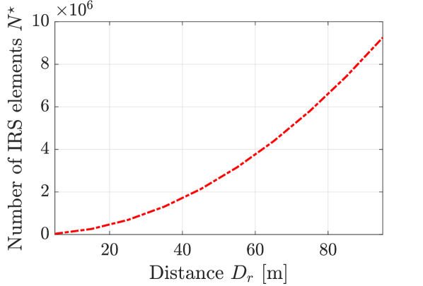
Figure 6: Number of IRS elements $N^{\star}$ versus distance $D_{r}$ for $\alpha=2$; $\mathbf{p}_{t}=(0,-0.6,1)$, $\mathbf{p}_{r}=(0,D_{r},1)$, IRS at $(0,(D_{r}-y_{t})/2,1)$ with $y_{t}=-0.6$, $f=300$ GHz, $\kappa_{\text{abs}}(f)=0.0033$ m^-1, and $L_{x}=L_{y}=\lambda/2$.

V Numerical Results

In this section, we assess the performance of IRS-aided THz communication through numerical simulations. For this purpose, we calculate the achievable rate as

$$R=B\log_{2}(1+\text{SNR}),$$ (33)

where $B$ is the signal bandwidth. Moreover, the EE is specified as $\text{EE}\triangleq R/P_{c}$.

V-A Energy Efficiency

We consider a MIMO setup with $N_{t}=N_{r}=100$ antennas, i.e., $10\times 10$-element planar arrays. From Fig. 5, we verify that the IRS-assisted system with $N_{t}=N_{r}=50$ antennas offers a two-fold EE gain. Consequently, an IRS can provide an alternative communication link, in addition to LoS, where the Tx and Rx employ a smaller number of antennas to communicate with each other, hence saving energy. Note, though, that the suggested benefits are valid when: 1) the power expenditure of IRS elements is negligible compared to that of conventional phase shifters; 2) the Tx operates near the IRS in order to have a reasonable number of reflecting elements $N^{\star}$; and 3) reflection losses are small [18].

V-B IRS Placement and Near-Field Beamfocusing

We now investigate the impact of the IRS position on the number of IRS elements $N^{\star}$. For the deployment in Fig. 5, $D_{t}$ is small, and hence $D^{2}_{r}\approx D^{2}_{t}+D^{2}_{d}$. Further, $\phi_{r}=\pi/2$ which gives $F(\theta_{t},\phi_{r},\theta_{r})=\cos^{2}\theta_{t}$. Then, (31) reduces to

$$N^{\star}=\alpha\frac{\lambda}{L_{x}L_{y}}\frac{D_{t}D_{r}}{\cos\theta_{t}\sqrt{D^{2}_{r}-D^{2}_{t}}}e^{-\frac{1}{2}\kappa_{\text{abs}}(f)(\sqrt{D^{2}_{r}-D^{2}_{t}}-D_{r}-D_{t})},$$ (34)

which takes the asymptotic value

$$N_{\max}^{\star}=\alpha\frac{\lambda}{L_{x}L_{y}}\frac{D_{t}}{\cos\theta_{t}}e^{\frac{1}{2}\kappa_{\text{abs}}(f)D_{t}}$$ (35)

as $D_{r}\to\infty$; this follows from $\sqrt{D^{2}_{r}-D^{2}_{t}}\approx D_{r}$ for $D_{r}\gg~{}D_{t}$. Thus, $N^{\star}$ is bounded for a fixed IRS position near the Tx. Due to symmetry, the same holds when the IRS is near the Rx. For instance, $N^{\star}_{\max}=10,880$ in Fig. 5. In contrast, when the IRS is deployed always in the middle of the Tx and Rx, $N^{\star}$ increases as $O(D_{t}D_{r})$. This scaling law is depicted in Fig. 6. Consequently, the IRS has to be close to the link ends in order to compensate for the severe propagation losses with a practical number of reflecting elements. Note that similar findings were reported in [17]. In this case, the Tx/Rx will be in the Fresnel zone of the IRS where near-field beamfocusing becomes the optimal processing strategy; otherwise, the EE gains previously discussed cannot be attained.

$$G =\frac{\left|\sum_{n=0}^{N_{x}-1}e^{-jk\frac{(nd_{x})^{2}(1-\cos^{2}\phi_{t}\sin^{2}\theta_{t})}{2D_{t}}}\right|^{2}}{N_{x}^{2}}\frac{\left|\sum_{m=0}^{N_{y}-1}e^{-jk\frac{(md_{y})^{2}(1-\sin^{2}\phi_{t}\sin^{2}\theta_{t})}{2D_{t}}}\right|^{2}}{N^{2}_{y}}$$

$$\approx\frac{\left|\sum_{n=0}^{N_{x}^{2}-1}e^{-jk\frac{nd_{x}^{2}(1-\cos^{2}\phi_{t}\sin^{2}\theta_{t})}{2D_{t}}}\right|^{2}}{N_{x}^{4}}\frac{\left|\sum_{m=0}^{N_{y}^{2}-1}e^{-jk\frac{md_{y}^{2}(1-\sin^{2}\phi_{t}\sin^{2}\theta_{t})}{2D_{t}}}\right|^{2}}{N_{y}^{4}}$$

$$=\left|D_{N_{x}^{2}}\left(\frac{2\pi}{\lambda}\frac{d_{x}^{2}(1-\cos^{2}\phi_{t}\sin^{2}\theta_{t})}{2D_{t}}\right)\right|^{2}\left|D_{N_{y}^{2}}\left(\frac{2\pi}{\lambda}\frac{d_{y}^{2}(1-\sin^{2}\phi_{t}\sin^{2}\theta_{t})}{2D_{t}}\right)\right|^{2}.$$ (22)

VI Conclusions and Future Work

We studied the channel modeling and performance of IRS-assisted THz communication. First, we introduced a spherical wave channel model and employed plate scattering theory to derive the path loss. We next showed that the path loss is nearly constant across the IRS thanks to its small physical size. However, due to the large number of reflecting elements with respect to the wavelength, the Fresnel zone of a THz IRS is of several meters. To this end, we analyzed the power gain under near-field beamfocusing and conventional beamforming, and proved the suboptimality of the latter. One implication of this is that the IRS needs to know the exact location of the Tx and/or Rx, rather than their angular information, to perform beamfocusing. Capitalizing on the derived model, we finally investigated the EE scaling law of IRS-aided MIMO, and showed that it can outperform MIMO. Numerical results consolidate the potential of IRSs for THz communication. For future work, it would be interesting to study the reflection matrix design for a multi-antenna Tx/Rx that operates in the Fresnel zone of the IRS, as well as pursue an EE analysis under hardware impairments and channel estimation overheads.

References

- [1] T. S. Rappaport et al., “Wireless communications and applications above 100 GHz: Opportunities and challenges for 6G and beyond,” IEEE Access, vol. 7, pp. 78729-78757, 2019.
- [2] J. Zhang et al., “Prospective multiple antenna technologies for beyond 5G,” IEEE J. Sel. Areas Commun., vol. 38, no. 8, pp. 1637–1660, Aug. 2020.
- [3] L. Yan, C. Han, and J. Yuan, “A dynamic array-of-subarrays architecture and hybrid precoding algorithms for terahertz wireless communications,” IEEE J. Sel. Areas Commun., vol. 38, no. 9, pp. 2041-2056, Sept. 2020.
- [4] E. Basar et al, “Wireless communications through reconfigurable intelligent surfaces,” IEEE Access, vol. 7, pp. 116753-116773, 2019.
- [5] Ö. Özdogan, E. Björnson, and E. G. Larsson, “Intelligent reflecting surfaces: Physics, propagation, and pathloss modeling,” IEEE Wireless Commun. Lett., vol. 9, no. 5, pp. 581-585, May 2020.
- [6] M. Najafi, V. Jamali, R. Schober, and H. V. Poor, “Physics-based modeling and scalable optimization of large intelligent reflecting surfaces,” IEEE Trans. Commun., Dec. 2020.
- [7] S. W. Ellingson, “Path loss in reconfigurable intelligent surface-enabled channels,” arXiv preprint arXiv:1912.06759, 2019.
- [8] W. Tang et al., “Wireless communications with reconfigurable intelligent surface: Path loss modeling and experimental measurement,” IEEE Trans. Wireless Commun., vol. 20, no. 1, pp. 421-439, Jan. 2021.
- [9] A. Z. Elsherbeni, F. Yang, and P. Nayeri, Reflectarray Antennas: Theory, Designs, and Applications. John Wiley and Sons, 2018.
- [10] Z. Wan, Z. Gao, M. Di Renzo, and M.-S. Alouini, “Terahertz massive MIMO with holographic reconfigurable intelligent surfaces,” IEEE Trans. Commun., Mar. 2021.
- [11] O. Yurduseven, S. D. Assimonis, and M. Matthaiou, “Intelligent reflecting surfaces with spatial modulation: An electromagnetic perspective,” IEEE Open J. Commun. Society, vol. 1, pp. 1256-1266, Aug. 2020.
- [12] F. Guidi and D. Dardari, “Radio positioning with EM processing of the spherical wavefront,” IEEE Trans. Wireless Commun., Jan. 2021.
- [13] C. A. Balanis, Advanced Engineering Electromagnetics, 2nd ed. John Wiley & Sons, 2012.
- [14] M. Di Renzo et al., “Smart radio environments empowered by reconfigurable intelligent surfaces: How it works, state of research, and the road ahead,” IEEE J. Sel. Areas Commun., vol. 38, no. 11, pp. 2450-2525, Nov. 2020.
- [15] C. A. Balanis, Antenna Theory: Analysis and Design, John Wiley & Sons, 2012.
- [16] Q. Wu and R. Zhang, “Intelligent reflecting surface enhanced wireless network via joint active and passive beamforming,” IEEE Trans. Wireless Commun., vol. 18, no. 11, pp. 5394-5409, Nov. 2019.
- [17] Q. Wu et al., “Intelligent reflecting surface aided wireless communications: A tutorial,” IEEE Trans. Commun., Jan. 2021.
- [18] S.-K. Chou, O. Yurduseven, H. Q. Ngo, and M. Matthaiou, “On the aperture efficiency of intelligent reflecting surfaces,” IEEE Wireless Commun. Lett., vol. 10, no. 3, pp. 599-603, Mar. 2021.