Interactions of solitary waves in the Adlam-Allen model

Abstract

We study the interactions of two or more solitary waves in the Adlam-Allen model describing the evolution of a (cold) plasma of positive and negative charges, in the presence of electric and transverse magnetic fields. In order to show that the interactions feature an exponentially repulsive nature, we elaborate two distinct approaches: (a) using energetic considerations and the Hamiltonian structure of the model; (b) using the so-called Manton’s method. We compare these findings with results of direct simulations, and identify adjustments necessary to achieve a quantitative match between them. Additional connections are made, such as with solitons of the Korteweg–de Vries equation. New challenges are identified in connection to this model and its solitary waves.

I Introduction

The field of nonlinear plasma physics has been a rich source of intriguing problems for the dynamics of solitary waves in integrable and nearly-integrable systems infeld ; konosk . In particular, the famous work of Zabusky and Kruskal kz , which initiated the explosion of interest in solitons by showing that the continuum limit of the Fermi-Pasta-Ulam-Tsingou model fpu ; fput is the Korteweg-de Vries (KdV) equation kdv , was a motivating theme for the work of Washimi and Taniuti tan . The latter one demonstrated that small-amplitude ion-acoustic waves in plasmas are also governed by the KdV model, hence solitonic excitations may be expected in this setting too. However, as indicated in the historical review of early studies of solitons allen3 , it was overlooked in the seminal works kz and tan , and in the extensive literature initiated by them (see, e.g., infeld ; Rem ; mjarecent ), that solitary waves were discovered in plasmas well before Refs. kz and tan . Indeed, a fundamental model put forth by Adlam and Allen in 1958 and 1960 aa1 ; aa2 constitutes, arguably, one of the earliest encounters of the realm of plasma physics with the concept of solitary waves.

The analysis presented in Refs. aa1 and aa2 concerns the spatiotemporal evolution of the distribution of electrons and ions in a magnetized plasma. In this setting, the spatial variation occurs only along the $x$-direction, the electric field acts along the $\left(x,y\right)$ plane, being subject to the Faraday’s and Gauss’ laws, while the (transverse) magnetic field acting along the $z$-direction obeys the Ampére’s law. The Newtonian spatiotemporal dynamics of a plasma consisting of positive and negative charges is affected by the forces created by the electric and magnetic fields. In this framework, starting from first principles and utilizing well-established approximations, such as the quasi-neutrality concept, a reduced system for plasma dynamics under the action of the electromagnetic field was derived aa1 ; aa2 . Ultimately, the resulting Adlam-Allen (AA) system of partial differential equations (PDEs) involved only two evolution equations for the (rescaled) magnetic field $B$ and inverse density $R$, in the $(1+1)$-dimensional setting aa1 ; aa2 (see Ref. allen4 for a recent recount of the topic).

The AA system is the starting point of the present work. In particular, in a recent study PRE this nonlinear model of plasma physics was revisited, and key properties of its solutions, including solitary and periodic waves, were examined. In addition to that, a connection of the AA model to the KdV equation was established (see also Ref. nairn ) through a multiscale reduction, and collisions of solitary waves were briefly addressed. In the present work, we aim to study interactions of solitary wave in the AA system in detail. It is well known that solitons in the KdV equation repel each other, and exact multi-soliton solutions can be obtained by means of the inverse-scattering transform (IST) method mjarecent ; whitham ; leveque . Studies of interactions of solitary wave in non-integrable models, relying upon the identification of their pairwise potential interaction or force manton , have been the subject of numerous studies; see, e.g., Ref. kivshar for an early review of relevant results.

On the basis of the reduction of the AA model to the KdV equation for weakly supersonic speeds of the solitary waves PRE , it is natural to expect repulsion between them in the AA system as well. However, the AA model does not have the integrable structure of the KdV, which provides exact multi-soliton solutions, therefore one needs to resort to asymptotic techniques, such as ones based on the Lagrangian/Hamiltonian structure of the model interaction , or others which directly address the system of PDEs and related conservation laws manton . Here, we leverage both of these approaches and conclude that they lead to the same conclusions for the repulsion of the solitary waves. We then go on to corroborate analytical predictions by means of direct simulations.

The subsequent presentation is organized as follows. In Section II, we present the physical and mathematical basis of the above-mentioned setup, including its Lagrangian and Hamiltonian structure and solitary-wave solutions. In Section III, we use the asymptotic form of the solitary waves and the Hamiltonian of the AA system to address the tail-tail interaction between solitary waves. In Section IV, we compare the predictions to numerical simulations and identify adjustments needed for a quantitative match between them. In Section V, we summarize our findings and highlight some directions for future studies. Finally, in the Appendix we provide an alternative systematic proof of our results for the interaction between solitary waves, by means of the so-called Manton method manton ; panos_inter . A second Appendix offers a perspective on a different, but also important type of interaction, namely that of a solitary wave with a localized defect.

II The model, its properties, and solitary waves

II.1 Introducing the AA model

The AA model introduced in Refs. aa1 ; aa2 describes the wave propagation in a cold magnetized collisionless electron-ion plasma. In particular, the thermal motion is negligible in comparison to velocities of the particles due to the wave motion, and collisions are also neglected due to the fact that the collision frequencies are small (i.e., the mean time between collisions is much larger than the time which an ion/electron spends in the wave). Electrons and ions in the plasma are subject to the action of the magnetic field applied in the $z$-direction, and there is an induced electric field in the $y$-direction, while the assumption of the quasi-neutrality is consonant with the presence of a weak electric field in the $x$-direction. The latter is true as long as the electron plasma frequency is much greater than the electron cyclotron frequency. Note that such a setting may find applications both in fusion research and in studies of astrophysical phenomena, such as the solar wind solar .

Adlam and Allen described how a large-amplitude stationary compressional magnetic-field pulse (or a train of pulses PRE ) can exist and be sustained in the collisionless plasma. In particular, adopting the Lagrangian coordinate system (moving with the pulse), they have found a nonlinear solution of such a model involving ions, electrons and the electric and magnetic fields. This solution corresponds to accumulation of the magnetic flux, which is sustained by the flow of the plasma across it. The particles’ velocities must be large enough, so that the ion Larmor radius is larger than the effective width $D$ of the magnetic pulse, and the electric field of the ions is able to pull the electrons across $D$. Then, $D$ turns out to be $\sim c/\omega_{p}$, i.e., on the order of the colisionless skin depth (with $c$ being the speed of light and $\omega_{p}$ the plasma frequency), and the strength of the magnetic pulse depends on the Alfvén Mach number $M_{A}$, which lies in the interval of $1\leq M_{A}\leq 2$ (see e.g. swanson ; stix ).

The AA system can be expressed in the following dimensionless form PRE (see also Ref. nairn ):

$$R_{tt}+\frac{1}{2}\left(B^{2}\right)_{xx} = 0,$$ (1)

$$B_{xx}-RB+R_{0}B_{0} = 0,$$ (2)

where the real functions $R(x,t)>0$ and $B(x,t)$ represent, respectively, the inverse plasma density and the magnetic field, while constants $R_{0}$ and $B_{0}$ are the density and magnetic field strength in the undisturbed plasma, respectively (note that the plasma is assumed to be initially uniform and steady, i.e., $B=B_{0}$, and $R=R_{0}$, at $t=0$). These constants also set the boundary conditions (b.c.) at infinity, i.e., $R\rightarrow R_{0}$ and $B\rightarrow B_{0}$ as $|x|\rightarrow\infty$; notice that $R_{0}$ and $B_{0}$ are related by the following equation,

$$R_{0}\equiv B_{0}^{2}/C^{2},$$ (3)

where $C$ is the characteristic speed of small-amplitude waves propagating on top of the background solution $R=R_{0}$, $B=B_{0}$; details of the derivation and scaling of the AA system can be found in Refs. aa1 ; aa2 ; PRE ; nairn .

As mentioned above, Adlam and Allen have found a class of large-amplitude hydromagnetic solitary waves which propagate in this setting. Their analytical treatment was inherently nonlinear, due to the consideration of finite-amplitude waves and self-localization effects. Therefore, this treatment differs from that of linear waves commonly appearing in textbooks on plasma waves (see, e.g., Refs. swanson ; stix ), according to which the (linear) small-amplitude waves are considered as weak perturbations propagating on top of a background equilibrium.

In this work, we also focus on the fully nonlinear version of the AA model. However, the finite-amplitude solitary waves that we consider here share their qualitative properties with small-amplitude fast magnetoacoustic Alfvén modes, as obtained from the linear theory, under the approxomation of the cold collisionless plasma swanson ; stix . In fact, these are compressional electromagnetic waves, propagating perpendicularly to the background magnetic field. The particle motion in the waves is in the direction transverse to the background magnetic field, with the electric and magnetic fields of the wave oriented perpendicular and parallel to the background magnetic field, respectively. The AA model describes the self-localization of the waves along the $x$-direction perpendicular to the background magnetic field (which lies along the $z$-direction). Furthermore, the Faraday’s law, in conjunction with the presence of the magnetic field, accounts for the $y$-component of the electric field, while the $x$-component of the latter obeys the Gauss’ law.

II.2 Solitary waves

It is convenient to eliminate the constant background from Eqs. (1)-(2, upon introducing the following definitions:

$$R\left(x,t\right)\equiv R_{0}+u(x,t),~{}B(x,t)\equiv B_{0}+w\left(x,t\right),$$ (4)

where the fields $u$ and $w$ satisfy vanishing b.c. at infinity, namely $u,w\rightarrow 0$ as $|x|\rightarrow\infty$. Then, the respectively transformed Eqs. (1) and (2) read PRE :

$$u_{tt}+\left(\frac{1}{2}w^{2}+B_{0}w\right)_{xx} = 0,$$ (5)

$$w_{xx}-R_{0}w-B_{0}u-uw = 0.$$ (6)

As shown in Ref. PRE (see also Ref. davis for an earlier similar analysis), Eqs. (5) and (6) possess an exact solitary-wave solution of the form:

$$w_{\mathrm{sol}} = \frac{2B_{0}}{C}\frac{v^{2}-C^{2}}{C+v\cosh\left(\frac{B_{0}\sqrt{v^{2}-C^{2}}}{Cv}\xi\right)},$$ (7)

$$u_{\mathrm{sol}} = -\frac{1}{v^{2}}\left(B_{0}w_{\mathrm{sol}}+\frac{1}{2}w_{\mathrm{sol}}^{2}\right),$$ (8)

$$\xi \equiv x-vt.$$ (9)

Here, $v$ is the solitary-wave’s velocity, which takes values in the interval of

$$C<v<2C.$$ (10)

The lower bound $C$ of $v$ is set by the necessary condition for the existence of the homoclinic orbit that corresponds to the exact solitary-wave solution (this homoclinic orbit occurs in the phase plane of the dynamical system stemming from Eqs. (5)-(6) once traveling-waves solutions are sought). In terms of the underlying physics, this condition means that the nonlinear solitary waves propagate at speeds higher than that of the linear-wave propagation in the system PRE . On the other hand, the upper bound $2C$ for $v$ in Eq. (10) follows from the requirement that the (inverse) density $R$ must be positive definite. While formal solutions exist past this threshold, they have no physical meaning.

II.3 The Lagrangian and Hamiltonian structure

Here, we aim to reveal the Lagrangian/Hamiltonian structure of the AA system. For this purpose, following Ref. Chalmers , it is relevant to define potential $U(x,t)$ of field $u\left(x,t\right)$,

$$u\equiv\partial U/\partial x.$$ (11)

The substitution of definition (11) in Eqs. (5) and (6) and subsequent integration of the former equation with respect to $x$ replaces Eqs. (5) and (6) by the following equations:

$$U_{tt}+\left(\frac{1}{2}w^{2}+B_{0}w\right)_{x}=0,$$ (12)

$$w_{xx}-R_{0}w-B_{0}U_{x}-wU_{x}=0,$$ (13)

where we have set the constant of integration (which, in principle, may be a function of time) equal to zero, as per the assumption that $U(x)$ and $w(x)$ vanish as $|x|\rightarrow\infty$.

Next, it is straightforward to see that Eqs. (12) and (13) can be derived from Lagrangian $\mathfrak{L}=\int_{-\infty}^{+\infty}\mathcal{L}dx$, with density

$$\mathcal{L}=\frac{1}{2}U_{t}^{2}+\frac{1}{2}w_{x}^{2}+\frac{1}{2}U_{x}w^{2}+B_{0}U_{x}w+\frac{1}{2}R_{0}w^{2}.$$ (14)

The respective Hamiltonian is $H=\int_{-\infty}^{+\infty}\mathcal{H}dx$, with density

$$\mathcal{H}=\frac{1}{2}U_{t}^{2}-\frac{1}{2}w_{x}^{2}-\frac{1}{2}U_{x}w^{2}-B_{0}U_{x}w-\frac{1}{2}R_{0}w^{2}.$$ (15)

To define an effective potential of the interaction of two solitary waves moving with equal velocities $v$, it is necessary to rewrite Eqs. (12) and (13), together with the Lagrangian and Hamiltonian densities (14) and (15), in the reference frame moving with velocity $v$, i.e., in terms of the $\tau=t$ and $\xi=x-vt$ variables, as:

$$U_{\tau\tau}-2vU_{\xi\tau}+v^{2}U_{\xi\xi}+\left(\frac{1}{2}w^{2}+B_{0}w\right)_{\xi}=0,$$ (16)

$$w_{\xi\xi}-R_{0}w-B_{0}U_{\xi}-wU_{\xi}=0,$$ (17)

and

$$\mathcal{L}_{\mathrm{moving}}=\frac{1}{2}U_{\tau}^{2}-vU_{\xi}U_{\tau}+\frac{v^{2}}{2}U_{\xi}^{2}+\frac{1}{2}w_{\xi}^{2}+B_{0}U_{\xi}w+\frac{1}{2}R_{0}w^{2}+\frac{1}{2}U_{\xi}w^{2},$$ (18)

$$\mathcal{H}_{\mathrm{moving}}=\frac{1}{2}U_{\tau}^{2}-\frac{v^{2}}{2}U_{\xi}^{2}-\frac{1}{2}w_{\xi}^{2}-B_{0}U_{\xi}w-\frac{1}{2}R_{0}w^{2}-\frac{1}{2}U_{\xi}w^{2}.$$ (19)

In what follows, we will introduce effective mass $M$ of the solitary wave. In that connection, we note that, in standard models, the solitary wave’s kinetic energy, which is produced by the integral, with respect to $\xi$, of the kinetic part of the Lagrangian density ($\int_{-\infty}^{+\infty}d\xi$), is kivshar :

$$E_{\mathrm{kin}}=\left(1/2\right)Mv^{2}.$$ (20)

III The interaction of far separated solitary waves

As is customary in studies of generic settings interaction ; manton ; panos_inter , a pair of interacting solitary waves separated by large distance $L$ is approximated by juxtaposing two identical solitary-wave solutions given by Eqs. (8) and (7). They interact via their exponentially decaying tails. Assuming that the center of the solitary wave is fixed at $\xi=0$, and taking into account that $\mathrm{sech}(x)\approx 2e^{-x}$ at $x\rightarrow\infty$, the expressions for the tails which are derived by (7) and (8) are:

$$w_{\mathrm{sol}} \approx \frac{4B_{0}}{Cv}\left(v^{2}-C^{2}\right)\exp\left(-\frac{B_{0}}{vC}\sqrt{v^{2}-C^{2}}|\xi|\right),$$ (21)

$$u_{\mathrm{sol}} \approx -\frac{B_{0}}{v^{2}}w_{\mathrm{sol}}=-\frac{4B_{0}^{2}}{Cv^{3}}\left(v^{2}-C^{2}\right)\exp\left(-\frac{B_{0}}{vC}\sqrt{v^{2}-C^{2}}|\xi|\right).$$ (22)

In turn, the use of Eq. (11) produces the respective asymptotic expression for the tail of field $U$:

$$U_{\mathrm{sol}}\approx\frac{4B_{0}}{v^{2}}\sqrt{v^{2}-C^{2}}\mathrm{sgn}\left(\xi\right)\exp\left(-\frac{B_{0}}{vC}\sqrt{v^{2}-C^{2}}|\xi|\right)+c_{\pm},$$ (23)

where $c_{\pm}$ are constant values at $\xi=\pm\infty$. The average value of the asymptotic constants, $(1/2)\left(c_{+}+c_{-}\right)$, is arbitrary, while the difference is uniquely determined by the solution as:

$$c_{+}-c_{-}=\int_{-\infty}^{+\infty}u_{\mathrm{sol}}(\xi)d\xi.$$ (24)

Next, we consider the pair of solitary waves with centers placed at positions $\xi_{0}=\pm L/2$, and the constant value of $U$ between them [see term $c_{\pm}$ in Eq. (23)] set equal to zero, so as to make the configuration symmetric. Then, an effective potential of the interaction between the far separated solitary waves, $W(L)$, can be derived by means of the general procedure elaborated in Ref. interaction . This is based on the substitution of the juxtaposition of the solitary waves in the expression for $H$, and handling terms with spatial derivatives by means of the integration by parts, so that the actual calculation of the integrals is not necessary, with all the contributions from the integrals being produced by the “surface terms” in the formula for the integration by parts. The result of this procedure is:

$$W(L)=\frac{32B_{0}^{3}}{C^{3}v^{3}}\left(v^{2}-C^{2}\right)^{5/2}\exp\left(-\frac{B_{0}}{vC}\sqrt{v^{2}-C^{2}}L\right),$$ (25)

with the positive sign of $W$ implying repulsion between the solitary waves. It is relevant to mention that, when calculating the effective potential (25), the result is produced by the third term in the Hamiltonian density (19), while the contributions from the second and fourth ones  exactly cancel each other. It should be noted here that the relation of the AA system to the KdV equation at speeds close to $C$ PRE , and the pairwise repulsion of KdV solitons kivshar is in line with the above analysis.

The repulsion, described above, will lead to an splitting of the initially equal velocities of the interacting solitary waves,

$$v\rightarrow v\pm\Delta v,$$ (26)

provided that $\Delta v$ represents a small perturbative effect. To obtain $\Delta v$ from the energy balance, it is necessary to know the exact expression for the energy of individual solitary waves. The substitution of the exact solitary wave solution given by Eqs. (8) and (7) in the expression for the Hamiltonian, determined by its density (15), leads to a very cumbersome expression. This expression becomes simpler in the limit case when the velocity is taken close to the solitary wave existence cutoff,

$$v-C\ll C.$$ (27)

Then, from Eqs. (7)-(9), we obtain

$$u_{\mathrm{sol}} \approx -\frac{2B_{0}^{2}}{C^{3}}\left(v-C\right)\mathrm{sech}^{2}\left(\frac{B_{0}\sqrt{v-C}}{\sqrt{2}C^{3/2}}\xi\right),$$ (28)

$$w_{\mathrm{sol}} \approx \frac{2B_{0}}{C}\left(v-C\right)\mathrm{sech}^{2}\left(\frac{B_{0}\sqrt{v-C}}{\sqrt{2}C^{3/2}}\xi\right),$$ (29)

$$H_{\mathrm{sol}} \approx \frac{8\sqrt{2}B_{0}^{3}}{3C^{5/2}}\left(v-C\right)^{3/2}.$$ (30)

The consideration of this case is relevant because the exponential smallness in Eq. (25) is less acute for small $\left(v-C\right)$. Note, in particular, that the $\mathrm{sech}^{2}$ limit corresponds to the soliton in the KdV limit of the AA system PRE .

Next, the interaction-induced change of the velocities, $\Delta v$, is determined by equating the interaction energy (25) to the difference between the energy of the two-solitary-wave configuration and the sum of individual energies of the two solitary waves, with the velocities split as per Eq. (26):

$$\Delta\left(H_{\mathrm{two~{}sol.}}\right)\approx\frac{\partial^{2}H_{\mathrm{sol}}}{\partial v^{2}}\left(\Delta v\right)^{2}\approx\frac{2\sqrt{2}B_{0}^{3}}{C^{5/2}\sqrt{v-C}}\left(\Delta v\right)^{2},$$ (31)

where condition (27) is used to simplify the expression, as it follows from Eq. (30). Finally, equation $\Delta\left(H_{\mathrm{two~{}sol.}}\right)=W(L)$ yields the result, which is valid under condition (27), provided that the result also satisfies the constraint $\Delta v\ll v-C$ (i.e., it is a small perturbative effect):

$$\Delta v\approx\frac{8}{\sqrt{C}}\left(v-C\right)^{3/2}\exp\left(-\frac{B_{0}\sqrt{v-C}}{\sqrt{2}C^{3/2}}L\right).$$ (32)

Note that, for fixed large $L$ and fixed $C$ and $B_{0}$, the interaction-induced velocity change, $\Delta v$, as given by Eq. (32) and considered as a function of $\left(v-C\right)$, attains a maximum (the strongest perturbative effect of the interaction) at

$$(v-C)|_{\max}=18C^{3}/\left(B_{0}L\right)^{2},$$ (33)

the maximum value itself being

$$\left(\Delta v\right)_{\max}=\left(\frac{6\sqrt{2}}{e}\right)^{3}\frac{C^{4}}{\left(B_{0}L\right)^{3}}\approx 30\frac{C^{4}}{\left(B_{0}L\right)^{3}}.$$ (34)

The above calculation, albeit approximate (especially since the velocity difference will keep changing as separation $L$ changes), suggests an important qualitative observation that is corroborated below by numerical computations. In particular, if we start from a symmetric configuration, it will progressively become asymmetric, leading to a pattern with taller and faster solitary waves on the right, and a shorter, slower solitary waves on the left. Below it is confirmed that, indeed, such a configuration in terms of heights and speeds is formed in the case of multi-solitary wave states.

In a quantitative form, the relative motion of interacting solitary waves obeys the dynamical equation,

$$\frac{d^{2}L}{d\tau^{2}}=-\frac{1}{M_{\mathrm{reduced}}}\frac{dW}{dL}.$$ (35)

Here, the reduced mass $M_{\mathrm{reduced}}$ of the solitary wave pair is considered to be

$$M_{\mathrm{reduced}}=(1/2)M,$$ (36)

where we have adopted the particle-like nature of the solitary wave, together with the standard result of the classical mechanics concerning the interaction of two point masses; thus, in Eq. (36), $M$ represents the above-mentioned mass of a single solitary wave, see Eq. (20). Actually, the calculation of $M$ is a central point in our analysis, as it concerns the comparison with numerical results (see next Section and Appendix B). We also note that the above approach to the the prediction of the evolution of the separation between the solitary waves is based on the energetics of the multi-solitary wave ansatz. A systematic analysis, including all the associated technical details at the level of the PDE system and conservation laws, generalizing another approach, introduced by Manton manton , is presented in Appendix A. We demonstrate that it leads to the same result as Eq. (35), thus confirming the above findings.

IV Numerical results

IV.1 The simulations

To perform a numerical study of the dynamics of interacting solitary waves in the AA model, we first consider a pair of solitary waves with equal velocities,

$$v_{1,2}(t=0)=1.1,$$ (37)

which are initially placed at $x_{1,2}(t=0)=\pm 10$, i.e., the initial distance between them is $L(0)=x_{1}(t=0)-x_{2}(t=0)=20$. In all simulations, we set $B_{0}=R_{0}=1$ (for this choice, the dimensionless form of the AA model considered here coincides with the one adopted in Ref. nairn ), which means $C=1$, see Eqs. (1)-(3). To apply the numerical method, the spatial variable was discretized by finite differences, and forward marching in time was performed. The finite-difference scheme in space was implemented taking into regard the coupling of a given site with second neighbors, in order to produce a stable numerical algorithm. The time-integration has been performed with the Runge-Kutta method of the $4^{\mathrm{th}}$-$5^{\mathrm{th}}$ order. To check the precision of the results, we used, as a diagnostic, the value of the total energy of the system calculated according to Eq. (15). Relative variance of the energy in all the simulations was $<10^{-6}$.

Since the physically relevant interval of the solitary-waves’ velocities is, according to (10), $1<v<2$, the selected value (37) is close to the lower edge of the interval. As can be inferred from Eqs. (8)-(7), the solitary waves in this velocity region are wide, which implies that their interaction is stronger; as a result, shorter integration times are required to let the interaction manifest itself.

The dynamical behavior of the two interacting solitary waves, in the co-travelling reference frame, is shown in Fig. 1. The symmetric configuration is quickly converted into one in which one solitary wave becomes taller (and consequently quicker) than the other. This is expected, as predicted by the analysis of the previous Section, since the repelling interaction of the solitary waves causes a change of their velocities, $\Delta v_{1}>0$ and $-\Delta v_{2}<0$, so that the velocities resulting from the interaction are

$$v_{1}=v_{1}(t=0)+\Delta v_{1}>v_{2}=v_{2}(t=0)-\Delta v_{2}.$$ (38)

The situation is reversed when we consider initial velocities with the opposite sign; in this case, the resulting configuration is a mirror image of Fig. 1 (not shown here).

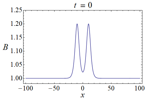
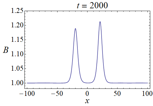
Figure 1: Results of simulations of the interaction of two solitary waves, as they are observed in the co-travelling reference frame for initial velocities $v_{1,2}(t=0)=1.1$ and positions $x_{1,2}(t=0)=\pm 10$. The two solitary waves, which initially have equal velocities, end up with different ones and, consequently, unequal heights.

Similar phenomenology is observed in the simulations if we consider more than two solitary waves placed symmetrically, with equal initial velocities. In particular, in Fig. 2 we display a four-solitary-wave configuration. In this case, the result shows a graded configuration of increasingly taller and faster solitary waves, that keep separating from each other in the course of the subsequent evolution.

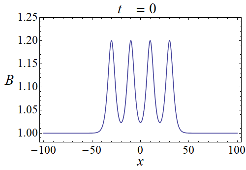
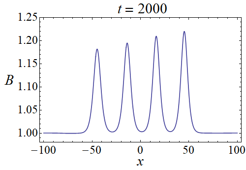
Figure 2: The result of the simulation of the set of four interacting solitary waves in the co-travelling reference frame. The initial velocities are $v_{1,2,3,4}(0)=1.1$, and their initial positions are $x_{1,4}(0)=\pm 30$ and $x_{2,3}(0)=\pm 10$. The solitary waves end up with different velocities and, consequently, different heights, cf. Fig. 1.

In addition, we have considered the evolution of solitary-wave sets with higher initial velocities (equal for all the pulses in the set, and with the same initial distance between them), taken in the range of $1.25\leqslant v(t=0)\leqslant 1.9$. We observed the same phenomenology but, as the width of the waves becomes smaller with the increase of $v$, the interaction becomes, accordingly, weaker and the corresponding dynamical response is slower than in the above case of $v(t=0)=1.1$.

IV.2 Comparison of the analytical estimate with numerical simulations

From the predicted form of the interaction potential (25) and expression (36) for the reduced mass, we derive the equation of motion for the distance between the two solitary waves:

$$\frac{d^{2}L}{d\tau^{2}}=-\frac{2}{M}\frac{d}{dL}W(L)=\frac{2A(v)}{M}\exp\left(-\lambda L\right),$$ (39)

where

$$A(v)\equiv\frac{32B_{0}^{4}}{C^{4}v^{4}}\left(v^{2}-C^{2}\right)^{3},\quad\lambda\equiv\frac{B_{0}}{vC}\sqrt{v^{2}-C^{2}}.~{}$$ (40)

A subtle issue in this connection is the identification of the mass $M$ of the solitary wave. Considering either the kinetic energy term in the Hamiltonian (for a stationary solitary wave in the co-traveling reference frame) and setting it equal to $(1/2)Mv^{2}$, or the momentum,

$$P=-\int_{-\infty}^{+\infty}U_{t}U_{x}dx,$$ (41)

and setting it equal to $Mv$, leads to the conclusion that

$$M=\int_{-\infty}^{+\infty}u^{2}dx.$$ (42)

In Appendix B we further explore this definition of the solitary wave’s mass, upon considering the dynamical response of the solitary wave to a perturbation represented by a potential term added to the system, which is also corroborated by direct numerical simulations.

Here it should be pointed out that the above expression for $M$ is not an intuitively evident one, as it refers solely to the mass associated with the $u$-component of the AA solitary wave, while the $w$-component does not contribute to the calculation of the mass, because Eq. (6) for this component does not contain time derivatives. In light of this fact, here we proceed in the following way: by numerically solving the ordinary differential equation (ODE) (39), we obtain distance $L$ between the two solitary waves as a function of time. This prediction is compared to the full numerical result, produced by simulations of the AA system, i.e., Eqs. (5) and (6). Assuming that the tail-tail interaction force, produced by both the energetic considerations and the Manton method (see Appendix A) adequately characterizes the exponential nature of the pairwise repulsion between the solitary waves, we then use the above semi-analytical prediction and its comparison to the full numerical results to “adjust” the proper expression for the mass. This approach reveals a relevant correction to the effective mass of the solitary wave.

As said above, we aim, first, to numerically integrate Eqs. (5) and (6) and thus obtain the distance between the interacting solitary waves as a function of time. For this purpose, we used velocities $v\geqslant 1.5$, to make the waves more well-separated and thus improve the accuracy of the comparison of the full numerical results with predictions of the ODE (39), where the constants and the “naively defined” solitary-wave’s mass are taken as per Eqs. (40) and (42), respectively. The results for $v=1.6$ are shown in Fig. 3, where the red solid and dashed blue lines show, respectively, the distance between the solitary waves, as obtained from the direct numerical integration of Eqs. (5) and (6), and predicted by the solution of the ODE (39). In this case, the discrepancy between the PDE and ODE results is obvious. Similar results are produced by the comparison at other values of the parameters.

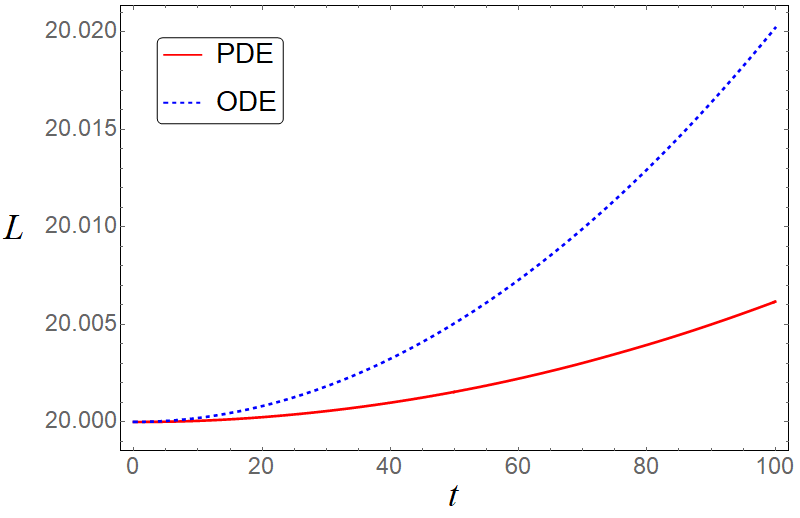
Figure 3: The comparison of the results for distance $L$ between the two interacting solitary waves in the co-travelling reference frame, for initial velocities $v_{1,2}(0)=1.6$. The (red) solid and (blue) dashed lines present the results produced, severally, by direct simulations of the underlying PDEs (5) and (6), and by the numerical solution of the effective ODE (39) with the constants taken as per Eq. (40) and (42).

Following the path outlined above, we attribute the discrepancy to the uncertainty regarding the solitary-wave’s mass. To fix the issue, we “phenomenologically” incorporate a fitting factor $\alpha(v)$ in Eq. (39), rewriting it as

$$\frac{d^{2}L}{d\tau^{2}}=\frac{A(v)}{M_{\mathrm{reduced}}^{\ast}}\exp\left(-\lambda L\right),\ \ \mathrm{with}\quad M_{\mathrm{reduced}}^{\ast}=\frac{M}{2\alpha(v)}.$$ (43)

Then, we determine the value of $\alpha(v)$ required for the PDE- and ODE-produced curves to match. The results are shown, for $v=1.6$ and other values of the initial velocities, in Fig. 4 and Table 1. In particular, for $v=1.6$ the two curves are made virtually identical by dint of the adjustment factor $\alpha=0.3045$ in Eq. (43). This observation and similar findings for other initial velocities confirm that the above analysis correctly captures the exponential decay of the inter-solitary-wave repulsive force, yet the straightforward theory misses the right prefactor in the respective equation of motion (39). In this connection, we stress that, for our analytis to be relevant for the comparison to the full simulations, we need the solitary waves to be well separated, in order apply the assumption of the tail-to-tail interaction, but not too far from each other either, lest the integration time, needed to make the interaction effect tangible, should be extremely large. In the present setting, we considered the initial separation of $L(0)=20$, and we did not observe any significant difference in the accuracy of the obtained results for larger separations.

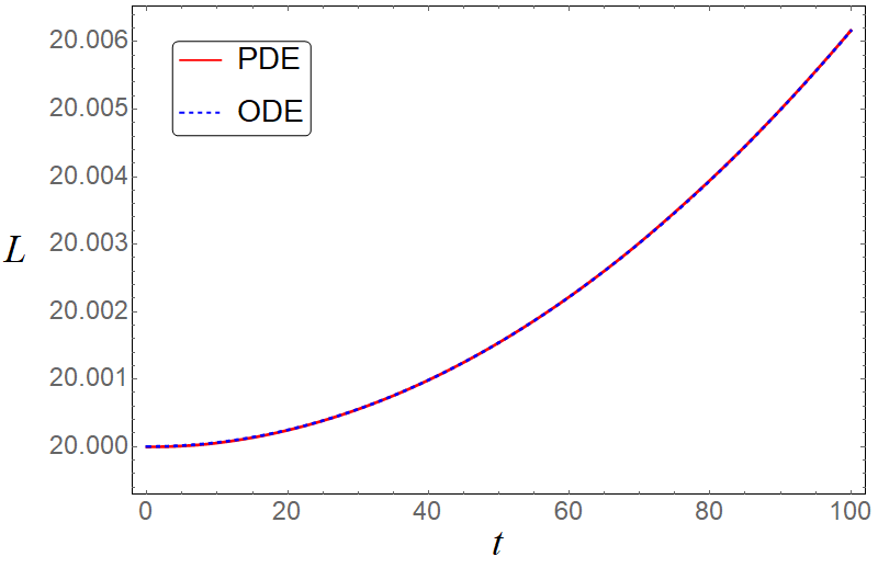
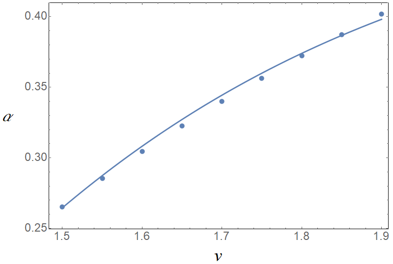
Figure 4: The left panel shows the comparison between the PDE results [solid (red) curve], the same as in Fig. 3), for distance $L(t)$ between the interacting solitary waves in the co-travelling reference frame, and the ODE counterpart [dashed (blue) curve], produced by Eq. (43) using the fitting prefactor $\alpha=0.3045$, in the case of $v_{1,2}(0)=1.6$. It is seen that this value of $2\alpha$ makes the two curves practically identical. The right panel shows, by means of the chain of dots, the fitting half-factor $\alpha$ for different values of the initial speed, as per the data presented in Table 1. The continuous curve plots an interpolating function (44), which approximates the values of $\alpha(v)$.

$v$	1.5	1.55	1.6	1.65	1.7	1.75	1.8	1.85	1.9
$\alpha$	0.2653	0.2855	0.3045	0.3227	0.34	0.3565	0.3724	0.3874	0.4019

Table 1: Values of the fitting half-factor $\alpha$ in Eq. (43) which provide the best match of $L(t)$ to the results of PDE simulations at different values of $v$.

To summarize these results, we sought a function $\alpha=\alpha(v)$ which may fit the data from Table 1. As it is seen in the right panel of Fig. 4, a reasonable choice is

$$\alpha(v)=1.05(v^{2}-C^{2})^{2}/v^{9/2}.$$ (44)

This function is built as a combination of powers of $(v^{2}-C^{2})$ and $v$, as these factors naturally appear in the calculation of the interaction force for the solitary waves. In Appendix B, we evaluate the relevance of considering the variation of the solitary wave mass in the context of the solitary wave-defect interaction.

V Conclusions

In the present work, we have revisited the Adlam-Allen (AA) model, governing the propagation of solitary waves in cold magnetized collisionless plasmas, in the presence of the electric field (in addition to an magnetic field). The AA model is one of the fundamental nonlinear models of plasma physics aa1 ; aa2 ; allen3 ; allen4 that has made the prediction of solitary waves possible, well before the (re-)discovery of the KdV equation and its celebrated solitons in the framework of the Fermi-Pasta-Ulam-Tsingou model. Indeed, the AA system is a source of localized and periodic waves, not only in the context of the transverse magnetic field applied to the plasmas, but also more recently for a longitudinal field gohar1 ; gohar2 .

Here, we have studied the interaction between solitary waves, a theme of substantial interest in the theory of solitary waves and solitons manton ; kivshar ; interaction . We provide the energy analysis, based on the Hamiltonian structure of the model, and complement it with a detailed derivation of the same result by means of an alternative (Manton’s) method, see Appendix. The resulting Newtonian dynamics for the separation clearly reveals the repulsive character of the interaction, as well as the exponential dependence of the force on the separation. This is natural to expect near the lower edge of the range (10) of accessible solitary wave speeds, where the model is close to the KdV limit (as shown earlier in Refs. PRE ; nairn ) and, thus, inherits the repulsive interaction between solitons which is well known in the framework of the KdV equation. Nevertheless, an essential element of uncertainty remains in the form of an accurate expression for the effective mass of the two-component solitary wave. We have side-stepped this uncertainty by finding a suitable velocity-dependent fitting factor, which takes values, roughly, between $2\alpha=0.5$ and $0.8$, which depends on the wave’s speed. This prefactor secures the full match between the ODE (semi-analytical) and PDE (fully numerical) results for the separation between the interacting solitary waves.

While our analysis provides a definitive explanation for the exponentially repulsive nature of the interactions, a remaining intriguing issue concerns the speed-dependent prefactor in the respective effective equation of motion fot the separation between the interacting solions. This amounts to an effective renormalization of the solitary-wave’s dynamical mass. The same issue also concerns the dynamics of the soliton gas in the AA system. A prototypical example of the latter was demonstrated in Fig. 2 for a configuration consisting of four interacting solitary waves, initially having equal velocities, which end up with different velocities and, consequently, different heights. This issue may also be relevant for other effectively nonlocal systems, in which one equation does not contain time derivatives (e.g., a Poisson-like equation). Systems of the latter type arise, in particular, in models of thermal media, plasmas, nematic liquid crystals, and Bose-Einstein condensates, see recent examples in works djf ; ECNU and references therein. Such systems, as well as higher-dimensional plasma models are natural objects for future work. Progress along these directions will be reported elsewhere.

Appendix A Derivation of the potential of the solitary waves interaction via Manton’s approach

Here, we aim to derive the interaction potential (25) by means of another approach, namely upon following the Manton’s method manton .

Introducing the traveling coordinate $\xi$, as per Eq. (9), in Eqs. (12)-(13) we obtain:

$$U_{\tau\tau}-2vU_{\xi\tau}+v^{2}U_{\xi\xi}+B_{0}w_{\xi}+\frac{1}{2}(w^{2})_{\xi}=0$$ (45)

$$w_{\xi\xi}-R_{0}w-B_{0}U_{\xi}-U_{\xi}w=0.$$ (46)

In the context of Klein-Gordon equations, the Manton’s method explores the evolution of momentum $P$ (as its time derivative is associated with the force, which here stems solely from the inter-solitary-wave interaction) manton . The expression for the field mommentum in the co-moving frame is given by

$$\tilde{P}=\int_{-\infty}^{+\infty}U_{\tau}U_{\xi}d\xi.$$ (47)

Differentiating the above expression momentum in time, we obtain:

$$\begin{array}[]{rcl}\displaystyle\frac{d\tilde{P}}{d\tau}&=&-\displaystyle\int_{-\infty}^{+\infty}\left(U_{\tau\tau}U_{\xi}+U_{\tau}U_{\xi\tau}\right)d\xi\\[12.0pt] &=&-\displaystyle\int_{-\infty}^{+\infty}\left[\left(2vU_{\xi\tau}-v^{2}U_{\xi\xi}-B_{0}w_{\xi}-\frac{1}{2}(w^{2})_{\xi}\right)U_{\xi}+U_{\tau}U_{\xi\tau}\right]d\xi\\[12.0pt] &=&\displaystyle\int_{-\infty}^{+\infty}\left[(B_{0}+w)w_{\xi}U_{\xi}~{}-\frac{1}{2}(U_{\tau}^{2})_{\xi}~{}{-v(U_{\xi}^{2})_{\tau}~{}+\frac{1}{2}v^{2}(U_{\xi}^{2})_{\xi}}\right]{d\xi}.\end{array}$$ (48)

In line with the original approach of manton , we proceed by considering two well-separated solitary waves, one placed at $x=0$ and the other one at $x=L\gg 0$. We also set two points, $x=a$ and $x=b$, with $a\rightarrow-\infty$ and $0\ll b\ll L$. Next, following Ref. manton , we neglect the two middle terms in the above equation, as we consider quasi-stationary solutions, and by using (12) we get:

$$\frac{d\tilde{P}}{dt}=-\int_{a}^{b}\left[(R_{0}w-w_{\xi\xi})w_{\xi}-\frac{v^{2}}{2}(u^{2})_{\xi}~{}\right]d\xi=\left[\frac{1}{2}w_{\xi}^{2}-\frac{1}{2}R_{0}w^{2}{+\frac{v^{2}}{2}u^{2}}\right]_{a}^{b}.$$ (49)

Now, we consider the superposition ansatz for the far separated solitary waves, $w=w_{1}+w_{2}$. We use the fact that the decay of the tails of the solitary waves is exponential. Thus, the contributions at $x=a$ vanish, while those at $x=b$ are of the form:

$$w_{1}\sim e^{-\lambda\xi}\quad\mathrm{and}\quad w_{2}\sim e^{\lambda(\xi-L)}.$$ (50)

Then, the contributions in (49) which are mixed (and consequently account for the interaction) are at point $x=b$,

$$\frac{d\tilde{P}}{d\tau}=w_{1_{\xi}}w_{2_{\xi}}-{R_{0}}w_{1}w_{2}+{v^{2}u_{1}u_{2}}.$$ (51)

The asymptotic form (21) and (22) yields

$$\left.\begin{array}[]{rcl}w_{1}&\approx&\displaystyle\frac{4B_{0}}{Cv}(v^{2}-C^{2})e^{-\lambda\xi}\\[10.0pt] w_{2}&\approx&\displaystyle\frac{4B_{0}}{Cv}(v^{2}-C^{2})e^{\lambda(\xi-L)}\end{array}\right\}\Rightarrow\begin{array}[]{rcl}w_{1{\xi}}&\approx&\displaystyle-\frac{4B_{0}^{2}}{C^{2}v^{2}}(v^{2}-C^{2})^{3/2}~{}e^{-\lambda\xi},\\[10.0pt] w_{2{\xi}}&\approx&\displaystyle\frac{4B_{0}^{2}}{C^{2}v^{2}}(v^{2}-C^{2})^{3/2}~{}e^{\lambda(\xi-L)},\end{array}$$ (52)

and

$$\begin{array}[]{rcl}u_{1}&\approx&\displaystyle-\frac{4B_{0}^{2}}{Cv^{3}}(v^{2}-C^{2})e^{-\lambda\xi},\\[10.0pt] u_{2}&\approx&\displaystyle-\frac{4B_{0}^{2}}{Cv^{3}}(v^{2}-C^{2})e^{\lambda(\xi-L)},\end{array}$$ (53)

with $\displaystyle\lambda=\left(B_{0}/Cv\right)\sqrt{v^{2}-C^{2}}$. Thus, by also using $\displaystyle R_{0}=B_{0}^{2}/C^{2}$, Eq. (51) reads

$$\begin{array}[]{rl}\displaystyle\frac{d\tilde{P}}{d\tau}&=-\displaystyle\frac{16B_{0}^{4}}{C^{4}v^{4}}(v^{2}-C^{2})^{3}~{}e^{-\lambda L}-\frac{16B_{0}^{4}}{C^{4}v^{2}}(v^{2}-C^{2})^{2}~{}e^{-\lambda L}{+\frac{16B_{0}^{4}}{C^{2}v^{4}}(v^{2}-C^{2})^{2}~{}e^{-\lambda L},}\end{array}$$ (54)

or

$$\frac{d\tilde{P}}{d\tau}=-\displaystyle{\frac{32B_{0}^{4}}{C^{4}v^{4}}(v^{2}-C^{2})^{3}}~{}e^{-\lambda L}.$$ (55)

Then, according to Eq. (35), we get

$$\frac{d^{2}L}{d\tau^{2}}=\frac{1}{M_{\mathrm{reduced}}}\displaystyle\frac{32B_{0}^{4}}{C^{4}v^{4}}(v^{2}-C^{2})^{3}~{}e^{-\lambda L}.$$ (56)

For the potential, we get

$$W(L)=\displaystyle\frac{32B_{0}^{3}}{C^{3}v^{3}}(v^{2}-C^{2})^{5/2}~{}e^{-\lambda L}.$$ (57)

These expressions recover the results that were obtained in the main text via the energetic arguments [Eq. (25)], and thus corroborate the repulsive exponentially decaying interaction between the solitary waves, mediated by their tails.

Appendix B Interaction of the solitary wave with a parametric force

Our aim in the present Appendix is to study the interaction between a solitary wave of the system with a defect using Manton’s approach and to assess the relevance of mass variation during such an interaction. To do so, we introduce a perturbation term $F$ in Eq. (5), as follows:

$$u_{tt}+\left(\frac{1}{2}w^{2}+B_{0}w\right)_{xx}=F,\ \ \mathrm{with}\quad F\equiv f(x)u(x,t).$$ (58)

The reasoning behind this choice of perturbation and the form of $f(x)$ is the following. Arguably, one of the simplest possibilities is to define a spatially localized parametric drive which introduces a small localized perturbation to the motion of the solitary wave, and is compatible with the zero boundary conditions as $x\rightarrow\pm\infty$ (in fact, as $x\rightarrow\pm\tilde{L}/2$, where $\tilde{L}$ is the size of the integration domain). In particular, we select

$$f\equiv f_{0}\frac{\sinh\left(x/l\right)}{\cosh^{3}\left(x/l\right)}.$$ (59)

Here $f_{0}$ and $l$ characterize, respectively, the amplitude and width of the spatially localized parametric perturbation term. In the subsequent numerical investigation, we considered a solitary wave with velocity $v_{0}=1.7$, under the action of the perturbation of the above form, with $f_{0}=0.1$ and $l=1.5$.

To utilize the Manton’s approach, we use the system’s equation of motion written in terms of field $w$, potential $U$ and the co-traveling coordinates $(\xi,\tau)$. This way the system becomes

$$U_{\tau\tau}-2vU_{\xi\tau}+v^{2}U_{\xi\xi}+B_{0}w_{\xi}+\frac{1}{2}(w^{2})_{\xi}=\int_{-\infty}^{\xi}f\frac{\partial U}{\partial\xi^{\prime}}\,d\xi^{\prime}.$$ (60)

We recall that the momentum of the soliton in the moving frame is given by

$$\tilde{P}=-\int_{-\infty}^{\infty}U_{\tau}U_{\xi}\,d\xi,$$ (61)

and its derivative by

$$\frac{d\tilde{P}}{d\tau}=-\int_{-\infty}^{+\infty}U_{\tau\tau}U_{\xi}\,d\xi-\int_{-\infty}^{+\infty}U_{\tau}U_{\xi\tau}\,d\xi.$$ (62)

By substituting the $U_{\tau\tau}$ term from Eq. (60) into Eq. (62), we obtain

$$\begin{array}[]{rl}\displaystyle\frac{d\tilde{P}}{d\tau}=&\displaystyle-2v\int_{-\infty}^{+\infty}U_{\xi\tau}U_{\xi}d\xi+v^{2}\int_{-\infty}^{\infty}U_{\xi\xi}U_{\xi}\,d\xi+\int_{-\infty}^{+\infty}\left[B_{0}w_{\xi}+\frac{1}{2}(w^{2})_{\xi}\right]U_{\xi}\,d\xi\\[15.0pt] &\displaystyle-\int_{-\infty}^{+\infty}U_{\xi}\int^{\xi}f\frac{\partial U}{\partial\xi^{\prime}}\,d\xi^{\prime}\,d\xi-\int_{-\infty}^{+\infty}U_{\tau}U_{\xi\tau}\,d\xi.\end{array}$$ (63)

On the other hand, we assume that $U=U(\xi-\xi_{0}(\tau))$, which represents a traveling-wave solution with its (moving) center $\xi_{0}(\tau)$. This is the only essential assumption adopted for the current analysis, i.e., we are exploring the dynamics of an adiabatically varying solitary wave whose properties are slowly varying in the presence of the defect. Thus, we set $U_{\tau}=-U_{\xi}\,\dot{\xi_{0}}$ and from Eq. (61) we get, also using definition (42),

$$\tilde{P}=\dot{\xi_{0}}\int_{-\infty}^{\infty}U_{\xi}^{2}\,d\xi=\dot{\xi_{0}}\int_{-\infty}^{\infty}u^{2}\,d\xi=\dot{\xi_{0}}\,M$$ (64)

and, accordingly,

$$\frac{d\tilde{P}}{d\tau}=M\,\ddot{\xi_{0}}+\dot{M}\dot{\xi_{0}}$$ (65)

The right-hand sides of Eqs. (63) and (65) should match. Indeed, if we consider the numerical solution of the system for $U$, $w$ to the calculate mass $M$, we see in Fig. 5 that they match. Note that we only consider the evolution up to $\tau=10$, rather than the full time interval of the interaction between the solitary wave and the potential. This is done because when the solitary wave interacts fully with the defect, it is deformed (as it can be seen in Fig. 6 for $\tau=16$) and the adiabatic-traveling-wave assumption is no longer valid, broken by the emission of radiation, as observed in the bottom panels of Fig. 6. On the other hand, up to $\tau=10$ it is relevant to assume that only the tail of the solitary wave and defect’s potential interact, the shape of the wave being only adiabatically modified, in line with the underlying assumptions. In Figure 6, we consider the evolution in the co-moving frame, thus the main body of the solitary wave appears still, while the inhomogeneity moves with negative velocity $v^{\prime}=-1.7$.

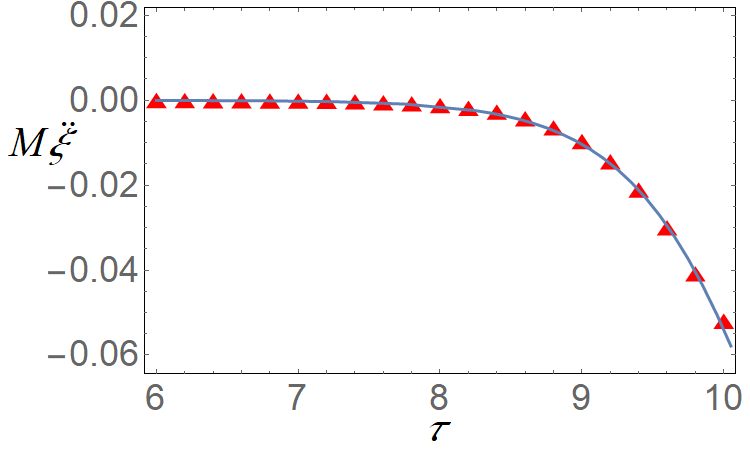
Figure 5: Comparison of the right-hand sides of Eqs. (63) and (65). The blue solid line and chain oif red triangles depict, respectively, the right-hand-sides of Eqs. (63) and (65).

Let us now evaluate terms contributing to the change of the momentum in the force balance associated with this problem. The contribution of the $\dot{M}\dot{\xi_{0}}$ term in Eq. (65) turns out to be negligible in comparison with the $M\ddot{\xi_{0}}$ one, being at least two orders of magnitude smaller than the latter one. For example, for $\tau^{\ast}=9.5$ we have $M(\tau^{\ast})\ddot{\xi_{0}}(\tau^{\ast})=-0.0251229$ and $\dot{\xi_{0}}(\tau^{\ast})\dot{M}(\tau^{\ast})=0.000109553$. Notice that in this setting the mass is evaluated to be: $M(\tau^{\ast})=1.7148755$, the acceleration is $\ddot{\xi}(\tau^{\ast})=-0.01465$, while the arising change in the mass is characterized by $\dot{M}(\tau^{\ast})=-0.0147101$ and $\dot{\xi}(\tau^{\ast})=-0.0251229$. It is thus concluded that, in the course of the time interval where this Manton-type method force balance is applicable, the variation of the mass is explicitly estimated to be $\approx 1\%$ in comparison to the actual solitary-wave mass, hence, for the time interval of our current considerations, the mass change does not substantially affect the wave-defect interaction.

Naturally, there remains an important open question whether the mass-fitting factor, used for the analysis of the of solitary-wave collisions, has some extension/connection to the mass variation in the wave-defect interaction. However, given the different nature of the two interactions (and the fact that we can only pursue the solitary-wave interaction until the substantial emission of radiation occurs, as explained in Figs. 5-6), this issue stays outside the purview of the present work.

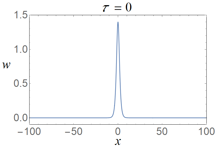
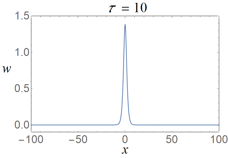
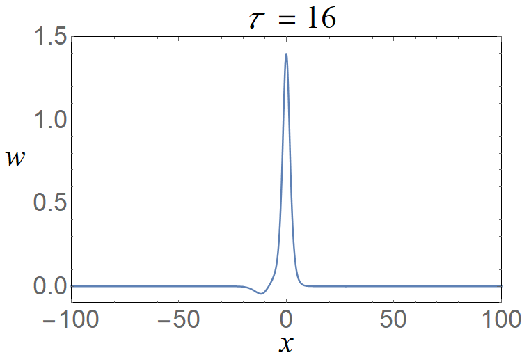
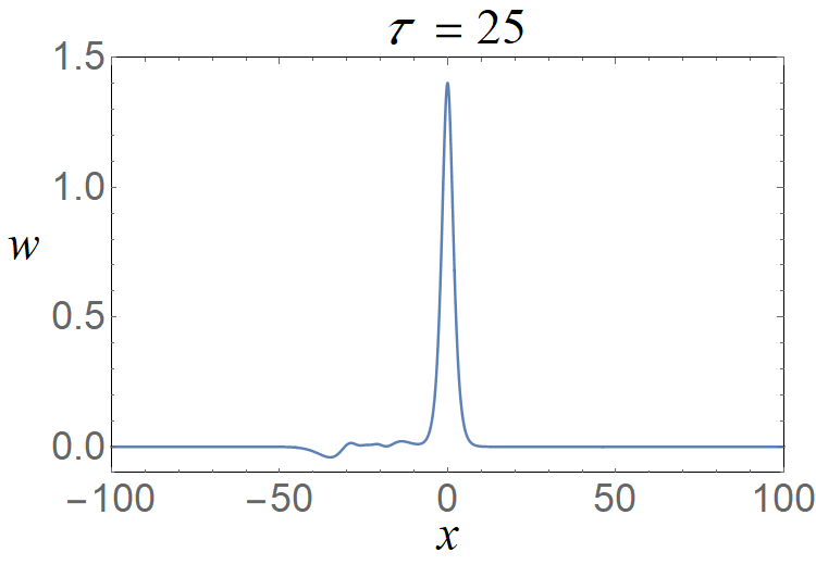
Figure 6: The interaction of the solitary wave with $v=1.7$ with the localized inhomogeneity introduced by Eq. (58) in the co-moving frame. The inhomogeneity is initially set at $x=20$. Up to $\tau=10$, the form of the wave remains practically intact. At $\tau=16$ we observe deformation of the wave, and at $\tau=25$ we observe the emergence of a small-amplitude shelf which, along with the accompanying tail, is attached to the (primary) solitary wave.

References

- (1) E. Infeld and G. Rowlands, Nonlinear Waves, Solitons and Chaos (Cambridge University Press Cambridge, 1990).
- (2) M. Kono and M. M. Skorić, Nonlinear Physics of Plasmas (Springer-Verlag, Heidelberg 2010).
- (3) N. J. Zabusky and M. D. Kruskal, Phys. Rev. Lett. 15, 240 (1965).
- (4) E. Fermi, J. Pasta, and S. Ulam, Tech. Rep. Los Alamos Nat. Lab. LA1940 (1955).
- (5) T. Dauxois, Phys. Today 61, 55 (2008).
- (6) D. J. Korteweg and G. de Vries, Phil. Mag. 39, 422 (1895).
- (7) H. Washimi and T. Taniuti, Phys. Rev. Lett. 17, 996 (1966).
- (8) J. E. Allen, Phys. Scripta 57, 436 (1998).
- (9) M. Remoissenet, Waves Called Solitons (Springer, Berlin, 1999).
- (10) M. J. Ablowitz, Nonlinear Dispersive Waves: Asymptotic Analysis and Solitons (Cambridge University Press, Cambridge, 2011).
- (11) J. H. Adlam and J. E. Allen, Philosophical Magazine 3, 448–455 (1958).
- (12) J. H. Adlam and J. E. Allen, Proc. Phys. Soc. 75, 640 (1960).
- (13) J. E. Allen, and J. Gibson, Phys. Plasmas 24, 042106 (2017).
- (14) J. E. Allen, D. J. Frantzeskakis, N. I. Karachalios, P. G. Kevrekidis, and V. Koukouloyannis, 102, 013209 (2020).
- (15) C. M. C. Nairn, R. Bingham, and J. E. Allen, J. Plasma Physics 71, 631 (2005).
- (16) G. B. Whitham, Linear and Nonlinear Waves (John Wiley, New York, 1974).
- (17) R. J. LeVeque, SIAM J. Appl. Math 47, 254 (1987).
- (18) B. A. Malomed, Phys. Rev. E 58, 7928 (1998).
- (19) N. S. Manton, Nuclear Phys. B 150, 397 (1979).
- (20) Yu. S. Kivshar and B. A. Malomed, Rev. Mod. Phys. 61, 763 (1989).
- (21) P. G. Kevrekidis, A. Khare and A. Saxena, Phys. Rev E 70, 057603 (2004).
- (22) N. Meyer-Vernet, Basics of the solar wind, (Cambridge University Press, Cambridge, 2007).
- (23) D. G. Swanson, Plasma Waves (Academic Press, London, 1989).
- (24) T. H. Stix, Waves in Plasmas (Springer Verlag, NY, 1992).
- (25) B. A. Malomed, D. Anderson, M. Lisak, M. L. Quiroga-Teixeiro, and L. Stenflo, Phys. Rev. E 55, 962-968 (1997).
- (26) L. Davis, R. Lüst, A. Schlüter, Z. Naturforschg. 13a, 916 (1958).
- (27) G. Abbas, J. E. Allen, M. Coppins, L. Simons, and L. James, Physics of Plasmas 27, 042102 (2020).
- (28) G. Abbas, P. G. Kevrekidis, J. E. Allen, V. Koukouloyannis, D. J. Frantzeskakis, and N. Karachalios, J. Phys. A: Math. Theor. 53, 425701 (2020).
- (29) T. P. Horikis and D. J. Frantzeskakis, Phys. Rev. Lett. 118, 243903 (2017).
- (30) J. Qin, Z. Liang, B. A. Malomed, and G. Dong, Phys. Rev. A 99, 023610 (2019).