CPHT-RR027.032021, March 2021

Wavefunction of the universe:
Reparametrization invariance and field redefinitions
of the minisuperspace path integral

Hervé Partouche,¹ Nicolaos Toumbas² and Balthazar de Vaulchier¹

¹ CPHT, CNRS, Ecole polytechnique, IP Paris,
F-91128 Palaiseau, France

² Department of Physics, University of Cyprus,
Nicosia 1678, Cyprus

  

Abstract

We consider the Hartle–Hawking wavefunction of the universe defined as a Euclidean path integral that satisfies the “no-boundary proposal.” We focus on the simplest minisuperspace model that comprises a single scale factor degree of freedom and a positive cosmological constant. The model can be seen as a non-linear $\sigma$-model with a line-segment base. We reduce the path integral over the lapse function to an integral over the proper length of the base and use diffeomorphism-invariant measures for the ghosts and the scale factor. As a result, the gauge-fixed path integral is independent of the gauge. However, we point out that all field redefinitions of the scale factor degree of freedom yield different choices of gauge-invariant path-integral measures. For each prescription, we compute the wavefunction at the semi-classical level and find a different result. We resolve in each case the ambiguity in the form of the Wheeler–DeWitt equation at this level of approximation. By imposing that the Hamiltonians associated with these possibly distinct quantum theories are Hermitian, we determine the inner products of the corresponding Hilbert spaces and find that they lead to a universal norm, at least semi-classically. Quantum predictions are thus independent of the prescription at this level of approximation. Finally, all wavefunctions of the Hilbert spaces of the minisuperspace model we consider turn out to be non-normalizable, including the no-boundary states.

1 Introduction

According to the inflationary paradigm, a tiny Planckian region of space underwent a period of rapid accelerated expansion, and grew large enough to encompass the entire observable universe. Quantum effects are crucial to understand the state of the universe at the initial stages of this inflationary era. Indeed, it is widely believed that quantum fluctuations seed the primordial density perturbations, which lead eventually to the large scale structure of the universe today. Hence, it would be desirable to obtain the wavefunction of the universe, and to uncover a statistical interpretation favouring initial conditions amenable for inflation.

A step toward this direction was initiated by Hartle and Hawking [1] in the context of Einstein’s theory of gravity for closed universes, in the presence of a positive cosmological constant $\Lambda>0$. In particular, they proposed a definition for the “ground-state wavefunction,” which Vilenkin has interpreted as the probability amplitude for creating from “nothing” a three-dimensional universe with metric $h_{ij}$ [2, 3, 4, 5]. In practice, this wavefunction is computed via a Euclidean path integral according to the “no-boundary proposal.” This path integral involves a sum over compact four-geometries that end on a particular spatial slice with induced metric $h_{ij}$. Notice that the denomination of “ground state” is somehow misleading, since in quantum gravity all states associated with a closed universe (including the matter content) are degenerate, with vanishing energy. Moreover, as we will see, such wavefunctions are not necessarily normalizable.

In this work, we address and clarify four issues related to this path integral approach to quantum gravity:

$(i)$ To begin with, since general relativity is invariant under diffeomorphisms, special attention must be paid to the gauge fixing of this symmetry. This problem can be analyzed in the simpler framework of minisuperspace models, where the universe is assumed to be homogeneous, with a finite number of degrees of freedom depending only on time. In the literature, this gauge fixing of time-reparametrizations has not always been implemented appropriately for wavefunctions of the universe defined as path integrals, since the results depend on the chosen gauges [6].

In the present work, we consider the simplest such minisuperspace model, corresponding to a homogenous and isotropic universe with a single dynamical degree of freedom, namely the scale factor $a$. The model can be interpreted as a non-linear $\sigma$-model, where Euclidean time parametrizes a base manifold which is a line segment. Thus the scale factor is a coordinate in a one-dimensional target space. After gauge fixing of the Euclidean-time reparametrizations, the path integral over the lapse function reduces to an integral over the moduli space of the base manifold, which is parametrized by the proper length $\ell$ of the line segment. Moreover, we use diffeomorphism-invariant path-integral measures for the Faddeev–Popov ghosts and the scale factor. The outcome is a gauge-fixed path integral consistently independent of the choice of gauge.

$(ii)$ Field redefinitions of the scale factor, $a=A(q)$, leave the classical action invariant. However, at the quantum level, the path-integral measures ${\cal D}a$ and ${\cal D}q$ are not equivalent, as they are related to each other by a Jacobian. Since the fields $a$ and $q$ correspond to different coordinate systems of the $\sigma$-model target space, there is no preferred choice among these measures. As a result, infinitely many acceptable definitions of wavefunctions exist, which are associated with all possible field redefinitions of the scale factor degree of freedom.

For each choice of path-integral measure ${\cal D}q$, we compute the ground-state wavefunction using the steepest-descent method. This amounts to deriving all instanton solutions $\bar{q}$ and the corresponding values of the modulus $\bar{\ell}$ of the base segment, and to computing the quantum fluctuations and modulus fluctuations around these solutions at quadratic order. This is achieved by evaluating functional determinants by applying and refining the methods presented in Ref. [7].

$(iii)$ Given a choice of measure ${\cal D}q$, the set of wavefunctions describing the allowed states of the universe are the solutions of a Wheeler–DeWitt equation [8], which is the quantum analogue of the vanishing of the classical Hamiltonian on shell. However, in the process of canonical quantization of the Hamiltonian, the question of the ordering of the canonically conjugate variables $q$ and $\pi_{q}$ gives rise to an ambiguity in the exact form of the Wheeler–DeWitt equation.

Thanks to our derivation of the ground-state wavefunctions via the steepest-descent method, we are able to compare the results with the solutions of the Wheeler–DeWitt equation found by applying the WKB approximation. This allows us to resolve the ambiguity of the equation at the semi-classical level for every choice of measure ${\cal D}q$ in the path integrals.

$(iv)$ A question related to points $(ii)$ and $(iii)$ arises then. Do the different choices of measures ${\cal D}q$ in the prescription of the wavefunctions, as well as the distinct associated Wheeler–DeWitt equations, lead to different quantum gravity theories with the same classical limits? We show that the answer to this question is negative, at least at the semi-classical level.

In fact, by imposing that the Hamiltonians of these possibly distinct quantum theories are Hermitian, we find that the inner products of the corresponding Hilbert spaces take different forms in each case. However, the point is that the norms of the wavefunctions in the WKB approximation turn out to be universal, i.e. independent of the prescription. A non-trivial crosscheck of our results is provided by the particular choice of measure ${\cal D}q$ associated with a field $q$ with a quadratic kinetic term. In that case we find that the Wheeler–DeWitt equation reduces to the time-independent Schrödinger equation for vanishing energy, and that the inner product of the Hilbert space takes the standard form encountered in quantum mechanics.

Moreover, in the minisuperspace model that comprises a single scale factor degree of freedom, it turns out that all wavefunctions of the two-dimensional Hilbert space are non-normalizable, including that of the “ground-state.” To construct normalizable states, extra degrees of freedom must be added, rendering the dimension of the Hilbert space infinite. In some cases, it could then be possible to construct square-integrable wavefunctions by superimposing infinitely many solutions of the Wheeler–DeWitt equation [8].

Other seminal work on the wavefunction of the universe via the no-boundary proposal includes Refs. [9, 10, 11, 12, 13, 14, 15, 16, 17, 18, 19].

In Sect. 2, we review the definition of the ground-state wavefunction in the minisuperspace model we consider. The implementation of the gauge fixing of the Euclidean-time diffeomorphisms introduces a Faddeev–Popov Jacobian. The latter is expressed in Sect. 3 as a path integral over anticommuting ghosts, which is evaluated by using gauge-invariant measures. The outcome of the computation is that the Faddeev–Popov determinant is a trivial (and irrelevant) constant. The following two sections are devoted to the evaluation of the gauged-fixed path integral by applying the steepest-descent method. This is done in Sect. 4 by using the measure ${\cal D}a$ of the scale factor, while in Sect. 5 the result is generalized to any choice of gauge-invariant measure ${\cal D}q$ associated with a field $q$ obtained by redefining the scale factor degree of freedom. We also clarify the extent to which our calculations differ with previous works such as Refs. [15, 16, 6, 14], leading to different results. In Sect. 6, we lift at the semi-classical level the ambiguities arising in the Wheeler–DeWitt equations corresponding to the wavefunctions with arbitrary prescriptions ${\cal D}q$ for the path-integral measure. The equivalence at this level of approximation of all Hilbert spaces is demonstrated in Sect. 7. Our conclusions and perspectives can be found in Sect. 8. Various technical complements are reported in the Appendix.

2 Ground state wavefunction

In this section, we present the formal definition of the ground-state wavefunction of a closed, homogeneous and isotropic universe. The wavefunction is expressed in terms of a Euclidean path integral over the lapse function and the scale factor. Our goal is to carry out carefully the gauge fixing of the Euclidean-time reparametrization group. In the following sections we present the computations of the Faddeev–Popov determinant and the path integral over the scale factor.

2.1 Minisuperspace of dimension one

We are interested in Einstein’s theory for spatially-closed universes in the presence of a positive cosmological constant $\Lambda>0$, formulated on Lorentzian four-manifolds ${\cal M}$ with space-like boundaries $\partial{\cal M}$. The appropriate action reads

$$S =S_{\rm bulk}+S_{\rm boundary}\,,$$

$$\mbox{where}\quad S_{\rm bulk} =\int_{\cal M}{\rm d}^{4}x\,\sqrt{-g}\,\Big{[}{R\over 2}-\Lambda\Big{]}\,,\quad S_{\rm boundary}=-\int_{\partial{\cal M}}{\rm d}^{3}x_{\rm b}\,\sqrt{h}\,K\,,\phantom{\!\!\overset{\displaystyle|}{|}}$$ (2.1)

where $R$ is the scalar curvature associated with the metric $g_{\mu\nu}(x)$ on ${\cal M}$, while $K$ is the trace of the extrinsic curvature on $\partial{\cal M}$ whose metric is denoted $h_{ij}(x_{\rm b})$.

In this work, we consider the minisuperspace version where the degrees of freedom are reduced to a single scale factor depending only on time, $a(x^{0})$. This amounts to restricting the manifolds ${\cal M}$ to be homogeneous and isotropic. The invariant infinitesimal length squared is given by

$${\rm d}s^{2}=-N(x^{0})^{2}({\rm d}x^{0})^{2}+a(x^{0})^{2}\,{\rm d}\Omega_{3}^{2}\,,$$ (2.2)

where $N(x^{0})\equiv\sqrt{g_{00}(x^{0})}$ is the lapse function and ${\rm d}\Omega_{3}$ is the volume element of the unit 3-sphere. Moreover, $\partial{\cal M}$ is composed of 3-spheres at initial and final times $x^{0}_{\rm i}$ and $x^{0}_{\rm f}$, and the boundary action becomes

$$S_{\rm boundary}=3v_{3}\bigg{[}{a^{2}\over N}\,{{\rm d}a\over{\rm d}x^{0}}\bigg{]}_{x^{0}_{\rm i}}^{x^{0}_{\rm f}}\,\,,$$ (2.3)

where $v_{3}=2\pi^{2}$ is the volume of the unit 3-sphere. This term cancels a similar boundary term generated upon integrating by parts the second derivative of the scale factor arising from the Ricci scalar. As a result, the full action is reduced to

$$S=3v_{3}\int_{x^{0}_{\rm i}}^{x^{0}_{\rm f}}{\rm d}x^{0}\,N\bigg{[}\!-\!{a\over N^{2}}\Big{(}{{\rm d}a\over{\rm d}x^{0}}\Big{)}^{2}+a-\lambda^{2}a^{3}\bigg{]}\,,\quad\mbox{where}\quad\lambda=\sqrt{\Lambda\over 3}\,.$$ (2.4)

Notice the negative sign of the kinetic energy compared to that of a conventional matter scalar field. In this form, the action is expressed in terms of a Lagrangian involving only the scale factor and its first derivative (along with $N$), which is suitable for canonical quantization, as well as for deriving classical equations of motion, keeping the scale factor fixed on the boundaries.

2.2 Ground-state wavefunction as a Euclidean path integral

The quantum state of the universe can be described by a wavefunction that depends on $h_{ij}$, defined as a path integral. Hartle and Hawking have proposed to sum over all manifolds ${\cal M}$ with a space-like boundary, on which the induced metric is $h_{ij}$ [1]. Specifying other conditions on the class of paths summed over amounts to characterizing the state. For the ground state, the Hartle–Hawking prescription is formulated in terms of the Euclidean action, while the four-manifolds should have no other boundary than that of metric $h_{ij}$. This is the “no-boundary proposal” for the ground-state wavefunction. It follows from this definition, that the wavefunction can be interpreted as the amplitude for creating the three-geometry from the empty set, i.e. from “nothing” [2, 3, 4, 5].

In minisuperspace, the boundary geometry is fully characterized by the scale factor $a_{0}$ on the boundary 3-sphere. As a result, a possible definition of the ground-state wavefunction is given by

$$\Psi(a_{0})=\int{{\cal D}g_{00}\over{\rm Vol}({\rm Diff}[g_{00}])}\int_{\textstyle\begin{subarray}{c}\!\!a_{\rm i}=0\\ \,a_{\rm f}=a_{0}\end{subarray}}\!\!{\cal D}a\;e^{-{1\over\hbar}S_{\rm E}[g_{00},a]}\,,$$ (2.5)

where we keep explicit the reduced Planck constant $\hbar$. The following comments are in order:

$\bullet$ Two possible prescriptions for the continuation to imaginary time have been advocated in the literature, given by

$$x^{0}=s\,i\,x^{0}_{\rm E}\,,\leavevmode\nobreak\ \leavevmode\nobreak\ \quad\mbox{where}\leavevmode\nobreak\ \leavevmode\nobreak\ \quad s\in\{1,-1\}\,.$$ (2.6)

Hartle and Hawking [1] take $s=-1$, while Vilenkin [2, 3, 4, 5, 13] and Linde [9] argue for $s=+1$. In various minisuperspace models, the predictions associated with the two choices can be drastically different. For instance, when the path integral is approximated by the steepest-decent method, with only one instanton solution taken into account, the wavefunction for $s=-1$ leads to the conclusion that the cosmological constant is likely to be null [10]. On the other hand, when $s=+1$ conditions amenable for inflation are favored [9, 20]. In the following, we consider both options, so that the Euclidean action $S_{\rm E}=-iS$ becomes

$$S_{\rm E}[g_{00},a]=3sv_{3}\int_{x^{0}_{\rm Ei}}^{x^{0}_{\rm Ef}}{\rm d}x^{0}_{\rm E}\,\sqrt{g_{00}}\,\bigg{[}a\,g^{00}\Big{(}{{\rm d}a\over{\rm d}x^{0}_{\rm E}}\Big{)}^{2}+V(a)\bigg{]}\,,$$ (2.7)

where we have defined

$$V(a)=a-\lambda^{2}a^{3}\,.$$ (2.8)

Moreover, the paths $a(x^{0}_{\rm E})$ must obey $a(x^{0}_{\rm Ef})\equiv a_{\rm f}=a_{0}$ and the “no-boundary condition” $a(x^{0}_{\rm Ei})\equiv a_{\rm i}=0$. Since both choices of $s$ yield actions $S_{\rm E}[g_{00},a]$ not bounded from below, special attention must be paid for defining convergent path integrals. We will come back to this issue in Sect. 4.3.

$\bullet$ The action $S_{\rm E}$ describes a non-linear $\sigma$-model where Euclidean time parametrizes a base manifold which is a segment of metric $g_{00}$, while the scale factor is a coordinate in a one-dimensional target space of metric

$$G_{aa}=6v_{3}a\,.$$ (2.9)

In other words, the system can be viewed as describing a worldline $a(x^{0}_{\rm E})$ in a dimension-one target minisuperspace, by analogy with the worldline trajectory of a particle in spacetime, or a worldsheet embedded in spacetime in string theory.

$\bullet$ The action being invariant under Euclidean-time reparametrizations, all diffeomorphism-equivalent metrics $g_{00}$ yield an overcounting of physically equivalent configurations. As a result, the path-integral measure ${\cal D}g_{00}$ must be divided by the volume of this group, which is denoted by ${\rm Diff}[g_{00}]$.

$\bullet$ For field configurations $a(x^{0})$ and $a(\xi(x^{0}))$, where $\xi\in{\rm Diff}[g_{00}]$, to be truly equivalent, the path-integral measure ${\cal D}a$ must be invariant under this symmetry group.

$\bullet$ However, diffeomorphism-invariant measures are not unique. The definition of the wavefunction in Eq. (2.5) uses a particular choice of coordinate in the target space, namely the scale factor. As a result, $\Psi(a_{0})$ is not equivalent to the wavefunction defined with the measure ${\cal D}q$, where $q=Q(a)$ is a field redefinition for an arbitrary function $Q$. This is despite the fact that such a transformation leaves the action invariant, as it corresponds to a change of coordinate in the target space. Since there is no preferred variable $q$ in the target space, there is no preferred measure ${\cal D}q$ in the definition of the wavefunction. All choices yield wavefunctions solving different Wheeler–DeWitt equations. In Sects. 5 and 6, we will determine the relations between all these avatars and see in Sect. 7 how they yield equivalent predictions, at least at the semi-classical level.

2.3 Gauge fixing of the Euclidean-time reparametrizations

In this subsection, we rewrite in a more practical way the path integral over the metrics $g_{00}$, which is weighted by the inverse of the volume of the diffeomorphism group.

For any metric $g_{00}$ defined on the domain $[x^{0}_{\rm Ei},x^{0}_{\rm Ef}]$, let us denote the action of a change of coordinate as follows,

$$\xi(x^{0}_{\rm E})=x^{\xi 0}_{\rm E}\,,\leavevmode\nobreak\ \leavevmode\nobreak\ \quad g^{\xi}_{00}(x^{\xi 0}_{\rm E})=\Big{(}{{\rm d}x^{0}_{\rm E}\over{\rm d}x^{\xi 0}_{\rm E}}\Big{)}^{2}\,g_{00}(x^{0}_{\rm E})\,,\leavevmode\nobreak\ \leavevmode\nobreak\ \quad a^{\xi}(x^{\xi 0}_{\rm E})=a(x^{0}_{\rm E})\,.$$ (2.10)

For an infinitesimal diffeomorphism $\xi={\rm Id}+\delta\xi$, this transformation rule yields

$$x^{\xi 0}_{\rm E}=x^{0}_{\rm E}+\delta x^{0}_{\rm E}\quad\Longrightarrow\quad\delta_{\xi}g_{00}=-2\nabla_{0}\delta x_{\rm E0}+{\cal O}(\delta x_{\rm E0}^{2})\,,$$ (2.11)

where $\nabla_{0}$ is the covariant derivative associated with $g_{00}$. Notice that not all metrics $g_{00}$ are equivalent up to diffeomorphisms since such transformations cannot change the proper length $\ell$ of the line segment,

$$\ell=\int_{x_{\rm Ei}}^{x_{\rm Ef}}{\rm d}x^{0}_{\rm E}\,\sqrt{g_{00}}=\int_{\xi(x_{\rm Ei})}^{\xi(x_{\rm Ef})}{\rm d}x^{\xi 0}_{\rm E}\,\sqrt{g^{\xi}_{00}}\,.$$ (2.12)

As a result, the set of metrics can be divided in equivalence classes distinguished by the value of $\ell\in\mathbb{R}_{+}$. In other words, a line segment admits a moduli space of real dimension one parametrized by $\ell$. In practice, varying the modulus of a metric $g_{00}$ amounts to rescaling it while keeping fixed its domain of definition.

Let us define reference metrics that will serve as gauge-fixed representatives of each equivalence class. We begin by choosing in class $\ell=1$ an arbitrary fiducial metric defined on a domain $[\hat{x}^{0}_{\rm Ei},\hat{x}^{0}_{\rm Ef}]$, which we denote by $\hat{g}_{00}[1]$. Then any class $\ell>0$ can be represented by the fiducial metric

$$\hat{g}_{00}[\ell]=\ell^{2}\,\hat{g}_{00}[1]\quad\mbox{defined on}\quad[\hat{x}^{0}_{\rm Ei},\hat{x}^{0}_{\rm Ef}]\,.$$ (2.13)

Any other metric $g_{00}$ in class $\ell$ can be obtained by the action of a diffeomorphism $\xi$ on $\hat{g}_{00}[\ell]$ (see Appendix A.1). However, such a coordinate transformation is not unique. For a base manifold of generic topology and dimension, there are continuous isometries, which by definition are diffeomorphisms that preserve the metric. In the case of a line segment, the group of isometries, or Killing group, is of dimension 0. It is nonetheless non-trivial and reduces to the $\mathbb{Z}_{2}$ generated by the discrete isometry that reverses the orientation of the segment. Both of these well known facts are derived in Appendix A.2. As a result, the group of diffeomorphisms can be divided into two disconnected components,

$${\rm Diff}[g_{00}]={\rm Diff}[g_{00}]_{{\rm Id}}\cup\big{(}\mbox{orientation reversal}\big{)}\!\cdot\!{\rm Diff}[g_{00}]_{{\rm Id}}\,,$$ (2.14)

where ${\rm Diff}[g_{00}]_{{\rm Id}}$ is the subgroup connected to the identity.

Next we replace the path integral over $g_{00}$ by two integrals: An integral over the moduli space and the other one over the orbit of each equivalence class, in order to cancel the volume of the diffeomorphism group. This operation yields a Jacobian that can be determined by applying the method of Faddeev and Popov, which is valid for any local symmetry group. Let us define the quantity $\Delta_{\rm FP}[g_{00}]$ by

$${1\over\Delta_{\rm FP}[g_{00}]}=\int_{0}^{+\infty}\!\!{\rm d}\ell\int_{{\rm Diff}[\hat{g}_{00}[\ell]]}\!\!{\cal D}\xi\;\delta\big{[}g_{00}-\hat{g}^{\xi}_{00}[\ell]\big{]}\,,$$ (2.15)

where $\delta$ stands for a “functional Dirac distribution,” vanishing when $g_{00}\neq\hat{g}^{\xi}_{00}[\ell]$. In other words, it vanishes when the domains of definition $[x^{0}_{\rm Ei},x^{0}_{\rm Ef}]$ and $[\xi(\hat{x}^{0}_{\rm Ei}),\xi(\hat{x}^{0}_{\rm Ef})]$ differ, or when $g_{00}$ and $\hat{g}^{\xi}_{00}[\ell]$ differ at any instance of time.

Using Eq. (2.15) in Eq. (2.5), we obtain

$$\Psi(a_{0}) =\int_{0}^{+\infty}\!\!{\rm d}\ell\int_{{\rm Diff}[\hat{g}_{00}[\ell]]}\!\!{\cal D}\xi\int{{\cal D}g_{00}\over{\rm Vol}({\rm Diff}[g_{00}])}\;\delta[g_{00}-\hat{g}^{\xi}_{00}[\ell]]\;\Delta_{\rm FP}[g_{00}]\int_{\textstyle\begin{subarray}{c}\!\!a_{\rm i}=0\\ \,a_{\rm f}=a_{0}\end{subarray}}\!\!{\cal D}a$$

$$\;\quad\exp\Big{\{}\!-\!{1\over\hbar}\int_{x^{0}_{\rm Ei}}^{x^{0}_{\rm Ef}}{\rm d}x^{0}_{\rm E}\,\sqrt{g_{00}}\;{\cal L}_{\rm E}(g_{00},a,\partial_{x^{0}_{\rm E}}a)\Big{\}}\,,\phantom{\!\!\overset{\displaystyle|}{|}}$$ (2.16)

where ${\cal L}_{\rm E}$ is the Euclidean Lagrangian density associated with the action $S_{\rm E}$. Performing the path integral over $g_{00}$ and renaming $a$ into $a^{\xi}$ leads to

$$\Psi(a_{0}) =\int_{0}^{+\infty}\!\!{\rm d}\ell\int_{{\rm Diff}[\hat{g}_{00}[\ell]]}\!\!{\cal D}\xi\;{1\over{\rm Vol}({\rm Diff}[\hat{g}^{\xi}_{00}[\ell]])}\;\Delta_{\rm FP}[\hat{g}^{\xi}_{00}[\ell]]\int_{\textstyle\begin{subarray}{c}\!\!a^{\xi}(\hat{x}^{\xi 0}_{\rm Ei})=0\\ \,a^{\xi}(\hat{x}^{\xi 0}_{\rm Ef})=a_{0}\end{subarray}}\!\!{\cal D}a^{\xi}$$

$$\;\quad\exp\Big{\{}\!-\!{1\over\hbar}\int_{\hat{x}^{\xi 0}_{\rm Ei}}^{\hat{x}^{\xi 0}_{\rm Ef}}{\rm d}\hat{x}^{\xi 0}_{\rm E}\,\sqrt{\hat{g}^{\xi}_{00}[\ell]}\;{\cal L}_{\rm E}\big{(}\hat{g}^{\xi}_{00}[\ell],a^{\xi},\partial_{\hat{x}^{\xi 0}_{\rm E}}a^{\xi}\big{)}\Big{\}}\,.\phantom{\!\!\overset{\displaystyle|}{|}}$$ (2.17)

In the above expression, the action is diffeomorphism invariant. As stressed in the previous subsection, we also use a scalar-field measure satisfying this symmetry (see Sect. 4.3 for an explicit construction at the semi-classical level),

$${\cal D}a^{\xi}\equiv{\cal D}a^{\xi}(\hat{x}^{\xi 0}_{\rm{\rm E}})={\cal D}a(\hat{x}^{0}_{\rm E})\equiv{\cal D}a\,,\quad\mbox{where}\quad\hat{x}^{\xi 0}_{\rm E}=\xi(\hat{x}^{0}_{\rm E})\,.$$ (2.18)

$\Delta_{\rm FP}[g_{00}]$ is also invariant under the action of the diffeomorphism group since

$${1\over\Delta_{\rm FP}[g^{\xi}_{00}]} =\int_{0}^{+\infty}\!\!{\rm d}\ell\int_{{\rm Diff}[\hat{g}_{00}[\ell]]}\!\!{\cal D}\xi^{\prime}\;\delta\big{[}g^{\xi}_{00}-\hat{g}^{\xi^{\prime}}_{00}[\ell]\big{]}$$

$$=\int_{0}^{+\infty}\!\!{\rm d}\ell\int_{{\rm Diff}[\hat{g}_{00}[\ell]]}\!\!{\cal D}\xi^{\prime}\;\delta\big{[}g_{00}-\hat{g}^{\xi^{-1}\circ\xi^{\prime}}_{00}[\ell]\big{]}$$

$$=\int_{0}^{+\infty}\!\!{\rm d}\ell\int_{{\rm Diff}[\hat{g}_{00}[\ell]]}\!\!{\cal D}\xi^{\prime\prime}\;\delta\big{[}g_{00}-\hat{g}^{\xi^{\prime\prime}}_{00}[\ell]\big{]}={1\over\Delta_{\rm FP}[g_{00}]}\,.$$ (2.19)

In the second line, we use the fact that the $\delta$-functional is diffeomorphism invariant, as will be seen explicitly in the next section. Moreover, the third line follows from the change of variable $\xi^{\prime\prime}=\xi^{-1}\circ\xi^{\prime}$ and the invariance of the measure, ${\cal D}\xi^{\prime}={\cal D}\xi^{\prime\prime}$, which is the case because the symmetry of reparametrizations is anomaly free. Finally, the group ${\rm Diff}[\hat{g}^{\xi}_{00}[\ell]]$ is by definition diffeomorphism invariant. As a result, the wavefunction simplifies to give

$$\Psi(a_{0}) =\int_{0}^{+\infty}\!\!{\rm d}\ell\int_{{\rm Diff}[\hat{g}_{00}[\ell]]}\!\!{\cal D}\xi\;{1\over{\rm Vol}({\rm Diff}[\hat{g}_{00}[\ell]])}\;\Delta_{\rm FP}[\hat{g}_{00}[\ell]]\int_{\textstyle\begin{subarray}{c}\!\!a(\hat{x}^{0}_{\rm Ei})=0\\ \,a(\hat{x}^{0}_{\rm Ef})=a_{0}\end{subarray}}\!\!{\cal D}a\;e^{-{1\over\hbar}S_{\rm E}[\hat{g}_{00}[\ell],a]}\,,$$ (2.20)

where the action is defined on the fixed domain of the fiducial metrics

$$S_{\rm E}\big{[}\hat{g}_{00}[\ell],a\big{]}=\int_{\hat{x}^{0}_{\rm Ei}}^{\hat{x}^{0}_{\rm Ef}}{\rm d}\hat{x}^{0}_{\rm E}\,\sqrt{\hat{g}_{00}[\ell]}\;{\cal L}_{\rm E}\big{(}\hat{g}_{00}[\ell],a,\partial_{\hat{x}^{0}_{\rm E}}a\big{)}\,.$$ (2.21)

All dependency on $\xi$ being now trivial, the path integral over the diffeomorphisms can be carried out, cancelling the volume factor. The ground-state wavefunction therefore takes the form of a gauged fixed path integral

$$\Psi(a_{0})=\int_{0}^{+\infty}\!\!{\rm d}\ell\;\Delta_{\rm FP}[\hat{g}_{00}[\ell]]\int_{\textstyle\begin{subarray}{c}\!\!a(\hat{x}^{0}_{\rm Ei})=0\\ \,a(\hat{x}^{0}_{\rm Ef})=a_{0}\end{subarray}}\!\!{\cal D}a\;e^{-{1\over\hbar}S_{\rm E}[\hat{g}_{00}[\ell],a]}\,.$$ (2.22)

In the following two sections, we first compute the Jacobian $\Delta_{\rm FP}[\hat{g}_{00}[\ell]]$ and then evaluate the path integral over the scale factor.

3 Faddeev–Popov Jacobian

Actually, the Faddeev–Popov determinant $\Delta_{\rm FP}[g_{00}]$ only depends on the equivalence class of its argument, thanks to its invariance under the diffeomorphism group. In what follows, however, we choose to keep the notation $\Delta_{\rm FP}[\hat{g}_{00}[\ell]]$. Our goal is to compute this Jacobian by expressing it as a path integral over ghost fields.

3.1 Introducing ghost fields

Since the reversal of the orientation of the segment is the only isometry, the path integral appearing in the expression

$${1\over\Delta_{\rm FP}[\hat{g}_{00}[\ell]]}=\int_{0}^{+\infty}\!\!{\rm d}\ell^{\prime}\int_{{\rm Diff}[\hat{g}_{00}[\ell^{\prime}]]}\!\!{\cal D}\xi\;\delta\big{[}\hat{g}_{00}[\ell]-\hat{g}^{\xi}_{00}[\ell^{\prime}]\big{]}$$ (3.23)

is twice the contribution of the diffeomorphisms connected to the identity,

$$\int_{{\rm Diff}[\hat{g}_{00}[\ell^{\prime}]]}\!\!{\cal D}\xi\leavevmode\nobreak\ \leavevmode\nobreak\ \longrightarrow\leavevmode\nobreak\ \leavevmode\nobreak\ 2\int_{{\rm Diff}[\hat{g}_{00}[\ell^{\prime}]]_{{\rm Id}}}\!\!{\cal D}\xi\,.$$ (3.24)

In that case, the $\delta$-functional enforces only $\ell^{\prime}=\ell$ and $\xi={\rm Id}$. In the vicinity of this point, the total variation of the fiducial metric is

$$\delta\hat{g}_{00}[\ell] \equiv\hat{g}^{{\rm Id}+\delta\xi}_{00}[\ell+\delta\ell]-\hat{g}_{00}[\ell]=\delta_{\xi}\hat{g}_{00}[\ell]+\partial_{\ell}\hat{g}_{00}[\ell]\delta\ell+\cdots$$

$$=-2\hat{\nabla}_{0}\delta x_{\rm E0}+2\hat{g}_{00}[\ell]\,{\delta\ell\over\ell}+\cdots\,,\phantom{\!\!\overset{\displaystyle|}{|}}$$ (3.25)

where we have used Eqs. (2.11) and (2.13), while $\hat{\nabla}$ is the covariant derivative with respect to $\hat{g}_{00}[\ell]$. As a result, we obtain

$${1\over\Delta_{\rm FP}[\hat{g}_{00}[\ell]]}=2\int{\rm d}\delta\ell\int_{\textstyle\begin{subarray}{c}\;\delta x^{0}_{\rm E}(\hat{x}^{0}_{\rm Ei})=0\\ \;\delta x^{0}_{\rm E}(\hat{x}^{0}_{\rm Ef})=0\end{subarray}}{\cal D}\delta x^{0}_{\rm E}\;\delta\Big{[}2\hat{\nabla}_{0}\delta x_{\rm E0}-2\hat{g}_{00}[\ell]{\delta\ell\over\ell}\Big{]}\,,$$ (3.26)

where the diffeomorphisms $\delta x^{0}_{\rm E}$ are required to vanish at the boundaries $\hat{x}^{0}_{\rm Ei}$ and $\hat{x}^{0}_{\rm Ef}$ of the domain of $\hat{g}_{00}[\ell]$. Otherwise the $\delta$-functional implies that they do not contribute at linear order.

By writing the $\delta$-functional as a Fourier transform, the previous expression becomes

$${1\over 2\,\Delta_{\rm FP}[\hat{g}_{00}[\ell]]}= \int{\rm d}\delta\ell\int_{\textstyle\begin{subarray}{c}\;\delta x^{0}_{\rm E}(\hat{x}^{0}_{\rm Ei})=0\\ \;\delta x^{0}_{\rm E}(\hat{x}^{0}_{\rm Ef})=0\end{subarray}}{\cal D}\delta x_{\rm E}\int{\cal D}\beta$$

$$\exp\Big{\{}2i\pi\int_{\hat{x}^{0}_{\rm Ei}}^{\hat{x}^{0}_{\rm Ef}}{\rm d}\hat{x}^{0}_{\rm E}\,\sqrt{\hat{g}_{00}[\ell]}\;\beta^{00}\Big{(}2\hat{\nabla}_{0}\delta x_{\rm E0}-2\hat{g}_{00}[\ell]{\delta\ell\over\ell}\Big{)}\Big{\}}\,,\phantom{\!\!\overset{\displaystyle|}{|}}$$ (3.27)

where the measure ${\cal D}\beta$ is assumed to be diffeomorphism invariant for the $\delta$-functional to be invariant as well. Notice that we have not made any reference to the contravariant or covariant nature of the tensors in the measures ${\cal D}\delta x_{\rm E}$ and ${\cal D}\beta$ because the contractions in the argument of the exponential can be made in an arbitrary way. We justify at the end of the section why this does not introduce ambiguities in the measures.

At this stage, it is relevant to introduce a notation that will be used extensively in the following. Let $f^{0\cdots 0}$ and $h^{0\cdots 0}$ be two tensors with $m\in\mathbb{Z}$ contravariant indices, where $m<0$ actually means that the tensors have $|m|$ covariant indices. We define the reparametrization-invariant quantity

$$(f,h)_{\ell}\equiv\int_{\hat{x}^{0}_{\rm Ei}}^{\hat{x}^{0}_{\rm Ef}}{\rm d}\hat{x}^{0}_{\rm E}\,\sqrt{\hat{g}_{00}[\ell]}\;f^{0\cdots 0}\,h^{0\cdots 0}\,\hat{g}_{00}[\ell]^{m}\,,$$ (3.28)

which we will especially use for $m=2$, $m=0$ and $m=-1$. To compute explicitly $\Delta_{\rm FP}[\hat{g}_{00}[\ell]]$ it is convenient to switch all integration variables into Grassmann ones,

$$\delta\ell\longrightarrow\lambda\,,\quad\leavevmode\nobreak\ \leavevmode\nobreak\ \delta x_{\rm E0}(\hat{x}^{0}_{\rm E})\longrightarrow c_{0}(\hat{x}^{0}_{\rm E})\,,\quad\leavevmode\nobreak\ \leavevmode\nobreak\ \beta^{00}(\hat{x}^{0}_{\rm E})\longrightarrow b^{00}(\hat{x}^{0}_{\rm E})\,,$$ (3.29)

where $b^{00}$ and $c_{0}$ are ghost fields. This operation inverts the r.h.s. of Eq. (3.27) up to an irrelevant numerical factor $\alpha$ [21]. Hence, we obtain

$$2\,\Delta_{\rm FP}[\hat{g}_{00}[\ell]] =\alpha\int_{\textstyle\begin{subarray}{c}\,c^{0}(\hat{x}^{0}_{\rm Ei})=0\\ \,c^{0}(\hat{x}^{0}_{\rm Ef})=0\end{subarray}}{\cal D}c\int{\cal D}b\int{\rm d}\lambda\;\exp\Big{\{}2i\pi\Big{(}b,2\hat{\nabla}c-2\hat{g}[\ell]{\lambda\over\ell}\Big{)}_{\ell}\Big{\}}$$

$$=4i\pi\alpha\int_{\textstyle\begin{subarray}{c}\,c^{0}(\hat{x}^{0}_{\rm Ei})=0\\ \,c^{0}(\hat{x}^{0}_{\rm Ef})=0\end{subarray}}{\cal D}c\int{\cal D}b\,\Big{(}b,{\hat{g}[\ell]\over\ell}\Big{)}_{\ell}\,\exp\Big{\{}4i\pi\,(b,\hat{\nabla}c)_{\ell}\Big{\}}\,,$$ (3.30)

where the second equality follows by Berezin integration over $\lambda$.

3.2 Choice of fiducial metric and mode expansions

Even though the content of this subsection can be obtained without specifying the fiducial metric, we find it simpler to present it for a convenient choice, remembering that $\Delta_{\rm FP}[\hat{g}_{00}[\ell]]$ is independent of this choice. So let us choose a constant lapse function,

$$\hat{g}_{00}[\ell](\tau)=\ell^{2}\quad\mbox{defined on}\quad[\hat{x}^{0}_{\rm Ei},\hat{x}^{0}_{\rm Ef}]=[0,1]\,,$$ (3.31)

where the variable $\hat{x}^{0}_{\rm E}$ is denoted $\tau$ for the sake of simplicity, while $\hat{\nabla}\equiv\partial_{0}$. Notice that $\tau$ is proportional to the “cosmological Euclidean time $t_{\rm E}$,” which satisfies ${\rm d}t_{\rm E}=\ell\,{\rm d}\tau$.

In Eq. (3.27), the paths $\beta^{00}(\tau)$ are arbitrary functions in $L^{2}([0,1])$, the vectorial space of functions that are square-integrable on $[0,1]$. Therefore, they can be expanded in the basis $\big{\{}1/\sqrt{2},\cos(k\pi\tau),k\in\mathbb{N}^{*}\big{\}}$. Likewise, the paths $\delta x_{\rm E0}(\tau)$ are functions in $L^{2}([0,1])$ obeying the boundary conditions $\delta x_{\rm E0}(0)=0$ and $\delta x_{\rm E0}(1)=0$. Hence, they can be expanded in the basis $\big{\{}\sin(k\pi\tau),k\in\mathbb{N}^{*}\big{\}}$. In order to keep track of the tensorial natures of the paths, it is preferable to view the vectorial spaces as Hilbert spaces respectively equipped with the inner products

$$(f,h)_{\ell}=\int_{0}^{1}{\rm d}\tau\ell\,f^{00}(\tau)h^{00}(\tau)\,(\ell^{2})^{2}\,,\qquad(f,h)_{\ell}=\int_{0}^{1}{\rm d}\tau\ell\,f_{0}(\tau)h_{0}(\tau)\,\ell^{-2}\,.$$ (3.32)

In that case, we can expand $\beta^{00}$, $\delta x_{\rm E0}$ and the ghost fields in orthonormal basis,

$$\beta^{00}(\tau) =\sum_{k\geq 0}\boldsymbol{\beta}_{k}\,\chi^{00}_{k}(\tau)\,,\qquad\delta x_{\rm E0}(\tau)=\sum_{k\geq 1}\boldsymbol{\gamma}_{k}\,\sigma_{0,k}(\tau)\,,$$

$$b^{00}(\tau) =\sum_{k\geq 0}\boldsymbol{\rm b}_{k}\,\chi^{00}_{k}(\tau)\,,\qquad\leavevmode\nobreak\ \leavevmode\nobreak\ \leavevmode\nobreak\ \,c_{0}(\tau)=\sum_{k\geq 1}\boldsymbol{\rm c}_{k}\,\sigma_{0,k}(\tau)\,,$$ (3.33)

where $\boldsymbol{\beta}_{k}$, $\boldsymbol{\gamma}_{k}$ and anticommuting $\boldsymbol{\rm b}_{k}$ and $\boldsymbol{\rm c}_{k}$ are arbitrary constants, while

$$\chi_{0}^{00}(\tau)=\ell^{-2}\,{1\over\sqrt{\ell}}\,,\quad\chi_{k}^{00}(\tau) =\ell^{-2}\sqrt{2\over\ell}\,\cos(k\pi\tau)\,,\leavevmode\nobreak\ \leavevmode\nobreak\ k\in\mathbb{N}^{*}\,,$$

$$\sigma_{0,k}(\tau) =\ell\,\sqrt{2\over\ell}\,\sin(k\pi\tau)\,,\leavevmode\nobreak\ \leavevmode\nobreak\ \leavevmode\nobreak\ \leavevmode\nobreak\ \,k\in\mathbb{N}^{*}\,,$$ (3.34)

satisfy

$$(\chi_{k},\chi_{k^{\prime}})=\delta_{kk^{\prime}}\,,\qquad(\sigma_{k},\sigma_{k^{\prime}})=\delta_{kk^{\prime}}\,.$$ (3.35)

Using these conventions, we first obtain two pieces of Eq. (3.30) which are

$$\Big{(}b,{\hat{g}[\ell]\over\ell}\Big{)}_{\ell}={\boldsymbol{\rm b}_{0}\over\sqrt{\ell}}\,,\qquad 4i\pi(b,\hat{\nabla}c)_{\ell}={4i\pi^{2}\over\ell}\sum_{k\geq 1}k\,\boldsymbol{\rm b}_{k}\boldsymbol{\rm c}_{k}\,.$$ (3.36)

Next, we determine the correctly normalized path-integral measures of the ghosts. In the case of commuting tensors $\beta^{00}$ and $\delta x_{\rm E0}$, the norms associated with the inner products in Eq. (3.32) yield

$$||\beta||_{\ell}^{2} \equiv(\beta,\beta)_{\ell}=\sum_{k\geq 0}\boldsymbol{\beta}_{k}^{2}\leavevmode\nobreak\ \leavevmode\nobreak\ \leavevmode\nobreak\ \leavevmode\nobreak\ \leavevmode\nobreak\ \leavevmode\nobreak\ \quad\Longrightarrow\leavevmode\nobreak\ \leavevmode\nobreak\ \leavevmode\nobreak\ \quad{\cal D}\beta=\bigwedge_{k\geq 0}{\rm d}\boldsymbol{\beta}_{k}\,,$$

$$||\delta x_{\rm E}||_{\ell}^{2} \equiv(\delta x_{\rm E},\delta x_{\rm E})_{\ell}\,=\sum_{k\geq 1}\boldsymbol{\gamma}_{k}^{2}\quad\Longrightarrow\quad{\cal D}\delta x_{\rm E}=\bigwedge_{k\geq 1}{\rm d}\boldsymbol{\gamma}_{k}\,.$$ (3.37)

In the anticommuting case of interest, we thus adopt the analogous prescriptions,

$${\cal D}b=\prod_{k\geq 0}{\rm d}\boldsymbol{\rm b}_{k}\,,\qquad{\cal D}c=\prod_{k\geq 1}{\rm d}\boldsymbol{\rm c}_{k}\,.$$ (3.38)

Taking into account these results, Eq. (3.30) becomes, up to an ambiguous sign that depends on the precise ordering of the Grassmann integration variables,

$$\Delta_{\rm FP}[\ell^{2}] =2i\pi\alpha\int{\rm d}\boldsymbol{\rm b}_{0}\,{\boldsymbol{\rm b}_{0}\over\sqrt{\ell}}\;\prod_{k\geq 1}\int{\rm d}\boldsymbol{\rm c}_{k}\,{\rm d}\boldsymbol{\rm b}_{k}\;e^{{4i\pi^{2}\over\ell}k\,\boldsymbol{\rm b}_{k}\boldsymbol{\rm c}_{k}}$$

$$={2i\pi\alpha\over\sqrt{\ell}}\prod_{k\geq 1}\!\Big{(}{4i\pi^{2}\over\ell}\,k\Big{)}$$

$$=\alpha\,\sqrt{2i\pi}\,,$$ (3.39)

where the last equality follows by the zeta regularization formulas

$$\prod_{k\geq 1}z={1\over\sqrt{z}}\,,\qquad\prod_{k\geq 1}k=\sqrt{2\pi}\,.$$ (3.40)

Remembering that $\Delta_{\rm FP}[\ell^{2}]$ is actually a Jacobian, $\alpha$ must be such that $\Delta_{\rm FP}[\ell^{2}]$ is a real non-negative number.

The important outcome of the above calculation is that the Jacobian is a trivial constant, i.e. it is independent of $\ell$. Note that this is not something that could be inferred at the outset, as this result applies to the case of a base manifold that is a segment in a specific way. Indeed, one can check that in the case of a base manifold with the topology of a circle, the Jacobian proves to be a constant times $1/\ell$, where $\ell$ is again the proper length of the circle [22].

To conclude this section, let us mention that since this is important, we make even clearer the independence of the Faddeev–Popov Jacobian on the choice of fiducial metric in Appendix A.4. Moreover, we would like to justify the claim below Eq. (3.27). The positions of the indices of $\beta^{00}$ and $\delta x_{\rm E0}$ appearing in the exponential in Eq. (3.27) have been chosen arbitrarily, since in all cases we would have been able to contract them by using the metric $\hat{g}_{00}[\ell]$. Hence, the tensor structure of the $b$-ghost could have been defined as $b^{00}$, $b^{0}_{0}$ or $b_{00}$, and likewise for the $c$-ghost as $c^{0}$ or $c_{0}$. However, since the mode expansions and the norms are always defined by using the “universal” scalar product in Eq. (3.28), the relations given in Eqs. (3.30), (3.36), (3.37), (3.38) are always valid and the final result of the Jacobian is unchanged. Therefore, there is no ambiguity in denoting the measures and scalar products without specifying which tensor structures are implicitly chosen.

4 Scale-factor path integral and modulus integral

Having implemented the gauge fixing of Euclidean-time reparametrizations, we now proceed to compute the path integral over the scale factor. We will work in the simplest gauge where the lapse function is constant, as displayed in Eq. (3.31). The expression of the wavefunction becomes

$$\Psi(a_{0})=\Delta_{\rm FP}\int_{0}^{+\infty}\!\!{\rm d}\ell\int_{\textstyle\begin{subarray}{c}\!\!a(0)=0\\ \,a(1)=a_{0}\end{subarray}}\!\!{\cal D}a\;e^{-{1\over\hbar}S_{\rm E}[\ell^{2},a]}\,,$$ (4.41)

where $\Delta_{\rm FP}$ is an irrelevant constant and the action (2.7) is

$$S_{\rm E}[\ell^{2},a]=3sv_{3}\int_{0}^{1}{\rm d}\tau\,\bigg{[}{a\over\ell}\Big{(}{{\rm d}a\over{\rm d}\tau}\Big{)}^{2}+\ell\,V(a)\bigg{]}\,.$$ (4.42)

Since the action is not quadratic, we will make use of the method of steepest-descent to approximate the evaluation of the wavefunction. In practice, one has to expand $S_{\rm E}[\ell^{2},a]$ around its extrema and integrate over the fluctuations at quadratic order only. The validity of this approximation is guaranteed when $\hbar\to 0$, which corresponds to the semiclassical limit. We would like to stress that our treatment to come differs to what is done in previous works [6, 14, 15, 16], as will be explained in Sect. 5.3.

4.1 Instanton solutions

In order to apply the method of steepest-descent, we extremize the action with respect to both $\ell$ and $a(\tau)$. Denoting such an extremum as $(\bar{\ell}^{2},\bar{a})$, we first have to solve

$$0=\!\left.{{\rm d}S_{\rm E}\over{\rm d}\ell}\right|_{(\bar{\ell}^{2},\bar{a})}=3sv_{3}\int_{0}^{1}{\rm d}\tau\,\bigg{[}\!-\!{\bar{a}\over\bar{\ell}^{2}}\Big{(}{{\rm d}\bar{a}\over{\rm d}\tau}\Big{)}^{2}+V(\bar{a})\bigg{]}\,.$$ (4.43)

Moreover, writing

$$a(\tau) =\bar{a}(\tau)+\delta a(\tau)\,,$$

$$\mbox{where}\quad\bar{a}(0) =0\,,\leavevmode\nobreak\ \leavevmode\nobreak\ \bar{a}(1)=a_{0}\quad\leavevmode\nobreak\ \leavevmode\nobreak\ \mbox{and}\leavevmode\nobreak\ \leavevmode\nobreak\ \quad\delta a(0)=0\,,\leavevmode\nobreak\ \leavevmode\nobreak\ \delta a(1)=0\,,$$ (4.44)

the equation of motion for the scale factor reads

$$0=\!\left.{\delta S_{\rm E}\over\delta a}\right|_{(\bar{\ell}^{2},\bar{a})}\leavevmode\nobreak\ \Longleftrightarrow\leavevmode\nobreak\ -{3\over\bar{a}^{2}}\Big{(}{{\rm d}\bar{a}\over{\rm d}\tau}\Big{)}^{2}-2{{\rm d}\over{\rm d}\tau}\Big{(}{1\over\bar{a}}\,{{\rm d}\bar{a}\over{\rm d}\tau}\Big{)}+{\bar{\ell}^{2}\over\bar{a}^{2}}\,V_{a}(\bar{a})=0\,,$$ (4.45)

where $V_{a}\equiv{\rm d}V/{\rm d}a$.

Particular solutions of Eq. (4.43) can be found by imposing the integrand to vanish identically, which amounts to solving the Friedmann equation. However, one may wonder whether more general solutions for which the integral vanishes while the integrand is non-zero are possible. It turns out that this is not the case. This can be inferred by noticing that the equation of motion for the scale factor is equivalent to

$$-{\bar{a}\over\bar{\ell}^{2}}\Big{(}{{\rm d}\bar{a}\over{\rm d}\tau}\Big{)}^{2}+V(\bar{a})={{\cal E}\over 3v_{3}}\,,$$ (4.46)

where ${\cal E}$ is an arbitrary integration constant, which can be related to the total energy of the universe. Using this relation, Eq. (4.43) gives $0=s{\cal E}$, showing that it suffices to solve the Friedmann equation in order to extremize the action with respect to $\ell$ and $a(\tau)$.

The latter equation takes the form

$$\left({{\rm d}(\lambda\bar{a})\over{\rm d}(\lambda\bar{\ell}\tau)}\right)^{2}+(\lambda\bar{a})^{2}=1\,,$$ (4.47)

with solution $\lambda\bar{a}(\tau)=|\sin(\lambda\bar{\ell}\tau+{\rm cst.})|$. Imposing $\bar{a}(0)=0$ implies the constant to be zero, while the condition $\bar{a}(1)=a_{0}$ fixes the modulus $\bar{\ell}$ of the base segment. When

$$\lambda a_{0}<1\,,$$ (4.48)

$\bar{\ell}$ can take discrete real values. However only two yield smooth instanton solutions,

$$\lambda\bar{a}_{\epsilon}(\tau) =\sin(\lambda\bar{\ell}_{\epsilon}\tau)\,,\quad\epsilon\in\{+1,-1\}\,,$$

$$\mbox{where}\quad\leavevmode\nobreak\ \leavevmode\nobreak\ \lambda\bar{\ell}_{+} =\arcsin(\lambda a_{0})\,,\quad\lambda\bar{\ell}_{-}=\pi-\arcsin(\lambda a_{0})\,.\phantom{\!\!\overset{\displaystyle|}{|}}$$ (4.49)

The line elements of the associated Euclidean spacetimes are

$$({\rm d}\bar{s}_{\rm E}^{\epsilon})^{2}={1\over\lambda^{2}}\Big{[}{\rm d}(\lambda\bar{\ell}_{\epsilon}\tau)^{2}+\sin(\lambda\bar{\ell}_{\epsilon}\tau)^{2}\,{\rm d}\Omega^{2}_{3}\Big{]}\,,\quad\tau\in[0,1]\,,$$ (4.50)

showing that the instantons describe portions of a 4-sphere of radius $1/\lambda$. Actually, $\epsilon=+1$ corresponds to a cap smaller than a hemisphere (see Fig. 1(a)), while $\epsilon=-1$ describes a cap bigger than a hemisphere (see Fig. 1(b)).

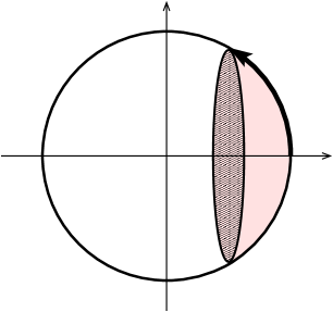
(a) Instanton solution $\bar{a}_{+}$ corresponding to the “small cap.”

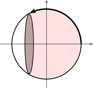
(b) Instanton solution $\bar{a}_{-}$ corresponding to the ‘‘big cap.”

Figure 1: The instanton solutions are portions of the 4-sphere of radius $1/\lambda$.

The actions associated with these solutions are

$$\bar{S}_{\rm E}^{\epsilon}=s\,{2v_{3}\over\lambda^{2}}\Big{[}1-\epsilon\big{(}1-(\lambda a_{0})^{2}\big{)}^{3\over 2}\Big{]}\,.$$ (4.51)

In this section, the semi-classical approximation of the wavefunction $\Psi(a_{0})$ will be carried out by applying the steepest-descent method to evaluate the path integral when $0<\lambda a_{0}<1$. The expression in the regime $\lambda a_{0}>1$ will be determined to some extent in Sect. 6 by analytically continuing the solutions of the Wheeler–DeWitt equation.

4.2 Expansion to quadratic order

The action (4.42) can be expanded around the extremal solutions $(\bar{\ell}_{\epsilon}^{2},\bar{a}_{\epsilon})$. Setting

$$\ell=\bar{\ell}_{\epsilon}+\delta\ell\,,\leavevmode\nobreak\ \leavevmode\nobreak\ \quad a(\tau)=\bar{a}_{\epsilon}(\tau)+\delta a(\tau)\,,$$ (4.52)

where $\delta a(\tau)$ obeys the boundary conditions of Eq. (4.44), one obtains to quadratic order

$$S_{\rm E}[\ell^{2},a]=\bar{S}_{\rm E}^{\epsilon}+3sv_{3}\int_{0}^{1}{\rm d}\tau\bar{\ell}_{\epsilon}\Big{[}\delta a\,{\cal Q}_{\epsilon}\delta a+2\,\delta a\,V_{a}(\bar{a}_{\epsilon})\,{\delta\ell\over\bar{\ell}_{\epsilon}}+{\delta\ell\over\bar{\ell}_{\epsilon}}\,V(\bar{a}_{\epsilon})\,{\delta\ell\over\bar{\ell}_{\epsilon}}\Big{]}\!+{\cal O}(\delta^{3})\,.$$ (4.53)

All linear terms vanish thanks to the equations of motion and ${\cal O}(\delta^{3})$ stand for terms at least cubic in fluctuations. In the above equation, ${\cal Q}_{\epsilon}$ is a quadratic differential operator,

$${\cal Q}_{\epsilon}=-{\bar{a}_{\epsilon}\over\bar{\ell}_{\epsilon}^{2}}\,{{\rm d}^{2}\over{\rm d}\tau^{2}}+{1\over\bar{\ell}_{\epsilon}^{2}}\,{{\rm d}\bar{a}_{\epsilon}\over{\rm d}\tau}\,{{\rm d}\over{\rm d}\tau}+{1\over 2}\,V_{aa}(\bar{a}_{\epsilon})\,.$$ (4.54)

Let us view the fluctuation $\delta a(\tau)$ as an element in the Hilbert space of $L^{2}([0,1])$ functions, obeying the boundary conditions $\delta a(0)=0$, $\delta a(1)=0$. This space is equipped with the inner product (see Eq. (3.28))

$$(\delta a_{1},\delta a_{2})_{\bar{\ell}_{\epsilon}}=\int_{0}^{1}{\rm d}\tau\bar{\ell}_{\epsilon}\,\delta a_{1}\,\delta a_{2}\,.$$ (4.55)

The linear operator ${\cal Q}_{\epsilon}$ can be seen as an endomorphism of this Hilbert space. Its adjoint, denoted ${\cal Q}_{\epsilon}^{\rm T}$, satisfies by definition

$$(\delta a_{1},{\cal Q}_{\epsilon}\delta a_{2})_{\bar{\ell}_{\epsilon}}=({\cal Q}_{\epsilon}^{\rm T}\delta a_{1},\delta a_{2})_{\bar{\ell}_{\epsilon}}$$ (4.56)

and can be determined by integrating by parts the left hand side,

$${\cal Q}_{\epsilon}^{\rm T}=-{\bar{a}_{\epsilon}\over\bar{\ell}_{\epsilon}^{2}}\,{{\rm d}^{2}\over{\rm d}\tau^{2}}-{3\over\bar{\ell}_{\epsilon}^{2}}\,{{\rm d}\bar{a}_{\epsilon}\over{\rm d}\tau}\,{{\rm d}\over{\rm d}\tau}-{2\over\bar{\ell}_{\epsilon}^{2}}\,{{\rm d}^{2}\bar{a}_{\epsilon}\over{\rm d}\tau^{2}}+{1\over 2}\,V_{aa}(\bar{a}_{\epsilon})\,.$$ (4.57)

Let us then introduce the “symmetric” and “antisymmetric” parts of ${\cal Q}_{\epsilon}$,

$${\cal S}_{\epsilon}={{\cal Q}_{\epsilon}+{\cal Q}^{\rm T}_{\epsilon}\over 2}\,,\leavevmode\nobreak\ \leavevmode\nobreak\ \quad{\cal A}_{\epsilon}={{\cal Q}_{\epsilon}-{\cal Q}^{\rm T}_{\epsilon}\over 2}\,.$$ (4.58)

They satisfy

$$(\delta a_{1},{\cal S}_{\epsilon}\delta a_{2})_{\bar{\ell}_{\epsilon}}=({\cal S}_{\epsilon}\delta a_{1},\delta a_{2})_{\bar{\ell}_{\epsilon}}\,,\leavevmode\nobreak\ \leavevmode\nobreak\ \quad(\delta a_{1},{\cal A}_{\epsilon}\delta a_{2})_{\bar{\ell}_{\epsilon}}=-({\cal A}_{\epsilon}\delta a_{1},\delta a_{2})_{\bar{\ell}_{\epsilon}}\,,$$ (4.59)

which means that ${\cal S}_{\epsilon}$ is self-dual while ${\cal A}_{\epsilon}$ satisfies $(\delta a,{\cal A}_{\epsilon}\delta a)_{\bar{\ell}_{\epsilon}}=0$ for all $\delta a$. As a result, we obtain

$$\delta a\,{\cal Q}_{\epsilon}\delta a=\delta a\,({\cal S}_{\epsilon}+{\cal A}_{\epsilon})\delta a=\delta a\,{\cal S}_{\epsilon}\delta a\,.$$ (4.60)

Using the explicit expression of the instanton solution in Eq. (4.49), the differential operator ${\cal S}_{\epsilon}$ can be written in the following form,

$${\cal S}_{\epsilon}=-{\bar{a}_{\epsilon}\over\bar{\ell}_{\epsilon}^{2}}\,{{\rm d}^{2}\over{\rm d}\tau^{2}}-{1\over\bar{\ell}_{\epsilon}^{2}}\,{{\rm d}\bar{a}_{\epsilon}\over{\rm d}\tau}\,{{\rm d}\over{\rm d}\tau}-2\lambda^{2}\bar{a}_{\epsilon}\,.$$ (4.61)

In the next subsection, we will show that the operator ${\cal S}_{\epsilon}$ is invertible when

$$0<\lambda a_{0}<1\,.$$ (4.62)

Assuming for the moment this fact, we can diagonalize the integrand appearing in Eq. (4.53) when $\lambda a_{0}$ is restricted in the above range,

$$\delta a\,{\cal S}_{\epsilon}\delta a+2\,\delta a\,V_{a}(\bar{a}_{\epsilon})\,{\delta\ell\over\bar{\ell}_{\epsilon}}+{\delta\ell\over\bar{\ell}_{\epsilon}}\,V(\bar{a}_{\epsilon})\,{\delta\ell\over\bar{\ell}_{\epsilon}} =\delta\check{a}\,{\cal S}_{\epsilon}\delta\check{a}+{\delta\ell\over\bar{\ell}_{\epsilon}}\big{[}V(\bar{a}_{\epsilon})-V_{a}(\bar{a}_{\epsilon}){\cal S}_{\epsilon}^{-1}V_{a}(\bar{a}_{\epsilon})\big{]}{\delta\ell\over\bar{\ell}_{\epsilon}}\,,$$

$$\mbox{where}\quad\delta\check{a} =\delta a+{\delta\ell\over\bar{\ell}_{\epsilon}}\,{\cal S}_{\epsilon}^{-1}V_{a}(\bar{a}_{\epsilon})\,.\phantom{\!\!\overset{\displaystyle|}{|}}$$ (4.63)

The above expressions deserve a comment. A priori, $V_{a}(\bar{a}_{\epsilon})$ is a function which satisfies

$$V_{a}(\bar{a}_{\epsilon})=1-3(\lambda\bar{a}_{\epsilon})^{2}\quad\Longrightarrow\quad V_{a}(\bar{a}_{\epsilon}(0))=1\,,\leavevmode\nobreak\ \leavevmode\nobreak\ V_{a}(\bar{a}_{\epsilon}(1))=1-3(\lambda a_{0})^{2}\,.$$ (4.64)

From this point of view, it does not belong to the Hilbert space of functions vanishing at $0$ and $1$, on which the endomorphisms ${\cal S}_{\epsilon}$ and ${\cal S}^{-1}_{\epsilon}$ act. However, we may consider this function on the open set $(0,1)$, and extend it so as to be odd on $(-1,0)\cup(0,1)$, and then 2-periodic on $\mathbb{R}\setminus\mathbb{Z}$. The Fourier series of the resulting function involves only the modes $\big{\{}\sqrt{2/\bar{\ell}_{\epsilon}}\sin(k\pi\tau),k\in\mathbb{N}^{*}\big{\}}$ and vanishes at every $\tau\in\mathbb{Z}$, where the function is discontinuous. Hence, in Eq. (4.63), $V_{a}(\bar{a}_{\epsilon})$ should be thought of as its Fourier expansion in the above basis, which indeed belongs to the Hilbert space.

Applying the steepest-decent method, the wavefunction in Eq. (4.41) reads

$$\Psi(a_{0})= \;\Delta_{\rm FP}\sum_{\epsilon=\pm 1}e^{-{1\over\hbar}\bar{S}_{\rm E}^{\epsilon}}\int{\rm d}\delta\ell\,\exp\Big{\{}\!-\!{3sv_{3}\over\hbar}\,{\cal K}_{\epsilon}\Big{(}{\delta\ell\over\bar{\ell}_{\epsilon}}\Big{)}^{2}\Big{\}}$$

$$\;\int_{\textstyle\begin{subarray}{c}\;\delta a(0)=0\\ \;\delta a(1)=0\end{subarray}}{\cal D}\delta a\,\exp\Big{\{}\!-\!{3sv_{3}\over\hbar}\,(\delta\check{a},{\cal S}_{\epsilon}\delta\check{a})_{\bar{\ell}_{\epsilon}}\Big{\}}\,(1+{\cal O}(\hbar))\,,$$ (4.65)

where we have defined

$${\cal K}_{\epsilon}=\int_{0}^{1}{\rm d}\tau\bar{\ell}_{\epsilon}\,\big{[}V(\bar{a}_{\epsilon})-V_{a}(\bar{a}_{\epsilon}){\cal S}_{\epsilon}^{-1}V_{a}(\bar{a}_{\epsilon})\big{]}\,.$$ (4.66)

Since ${\cal S}_{\epsilon}^{-1}V_{a}(\bar{a}_{\epsilon})$ belongs to the Hilbert space, so does $\delta\check{a}$. As a result, we may perform a change of variable (actually field redefinition) in the path integral from $\delta a$ to $\delta\check{a}$, with identical vanishing boundary conditions at $\tau=0$ and $\tau=1$. Furthermore, taking into account that the measures are related to each other by a trivial Jacobian

$${\cal D}\delta a={\cal D}\delta\check{a}\,\left|{{\cal D}\delta a\over{\cal D}\delta\check{a}}\right|={\cal D}\delta\check{a}\,,$$ (4.67)

we obtain that

$$\Psi(a_{0}) =\Delta_{\rm FP}\sum_{\epsilon=\pm 1}e^{-{1\over\hbar}\bar{S}_{\rm E}^{\epsilon}}\,Z_{\epsilon}(a_{0})\int{\rm d}\delta\ell\,\exp\Big{\{}\!-\!{3sv_{3}\over\hbar}\,{\cal K}_{\epsilon}\Big{(}{\delta\ell\over\bar{\ell}_{\epsilon}}\Big{)}^{2}\Big{\}}\,(1+{\cal O}(\hbar))$$

$$\mbox{where}\quad Z_{\epsilon}(a_{0}) =\int_{\textstyle\begin{subarray}{c}\;\delta\check{a}(0)=0\\ \;\delta\check{a}(1)=0\end{subarray}}{\cal D}\delta\check{a}\,\exp\Big{\{}\!-\!{3sv_{3}\over\hbar}\,(\delta\check{a},{\cal S}_{\epsilon}\delta\check{a})_{\bar{\ell}_{\epsilon}}\Big{\}}\,.\phantom{\!\!\overset{\displaystyle|}{|}}$$ (4.68)

4.3 Scale-factor quadratic fluctuations

For the sake of simplicity we make the change of notation $\delta\check{a}\to\delta a$ in the above expression of $Z_{\epsilon}(a_{0})$. Our goal in the present subsection is to compute this contribution to the wavefunction.

4.3.1 Mode expansion

Since ${\cal S}_{\epsilon}$ is a self-dual endomorphism of the Hilbert space, it is diagonalizable in an orthonormal basis. Denoting $\phi^{\epsilon}_{k}$ the eigenvector with eigenvalue $\nu_{k}^{\epsilon}$, we have

$${\cal S}_{\epsilon}\phi^{\epsilon}_{k}=\nu^{\epsilon}_{k}\phi^{\epsilon}_{k}\,,\leavevmode\nobreak\ \leavevmode\nobreak\ k\in\mathbb{N}^{*}\,,\quad\leavevmode\nobreak\ \leavevmode\nobreak\ \mbox{where}\leavevmode\nobreak\ \leavevmode\nobreak\ \quad(\phi^{\epsilon}_{k},\phi^{\epsilon}_{k^{\prime}})_{\bar{\ell}_{\epsilon}}=\delta_{kk^{\prime}}\,,\leavevmode\nobreak\ \leavevmode\nobreak\ \nu^{\epsilon}_{k}\in\mathbb{R}\,.$$ (4.69)

Expanding the scale factor fluctuation as

$$\delta a(\tau)=\sum_{k\geq 1}\boldsymbol{\delta\rm a}_{k}\,\phi^{\epsilon}_{k}(\tau)\,,$$ (4.70)

the path-integral measure is derived from the norm

$$||\delta a||_{\bar{\ell}_{\epsilon}}^{2}=(\delta a,\delta a)_{\bar{\ell}_{\epsilon}}=\sum_{k\geq 1}\boldsymbol{\delta\rm a}_{k}^{2}\quad\Longrightarrow\quad{\cal D}\delta a=\bigwedge_{k\geq 1}{\rm d}\boldsymbol{\delta\rm a}_{k}\,.$$ (4.71)

Hence, we obtain

$$Z_{\epsilon}(a_{0}) =\prod_{k\geq 1}\int{\rm d}\boldsymbol{\delta\rm a}_{k}\;e^{-{3sv_{3}\over\hbar}\nu^{\epsilon}_{k}(\boldsymbol{\delta\rm a}_{k})^{2}}=\prod_{k\geq 1}\sqrt{\hbar\,\pi\over 3sv_{3}\,\nu^{\epsilon}_{k}}$$

$$=\left({3sv_{3}\over\hbar\,\pi}\right)^{1\over 4}{1\over\sqrt{\det{\cal S}_{\epsilon}}}\,,$$ (4.72)

where the last equality follows by zeta regularization and $\det{\cal S}_{\epsilon}=\prod_{k\geq 1}\nu^{\epsilon}_{k}$. Notice that the prescription that we apply to the path integral is the following: Each mode coefficient $\boldsymbol{\delta\rm a}_{k}$ is integrated from $-\infty$ to $+\infty$ when $s\nu_{k}^{\epsilon}>0$, and from $-i\infty$ to $+i\infty$ when $s\nu_{k}^{\epsilon}<0$. As a result, all integrals are convergent. In fact, we will see at the end of the section that $\det{\cal S}_{+}$ and $\det{\cal S}_{-}$ have opposite signs. Hence, whatever choice of sign $s$ is made in the definition of Euclidean-time in (2.6), imposing domains of integration along the real and imaginary axes is necessary for both $Z_{+}(a_{0})$ and $Z_{-}(a_{0})$ to exist. In fact, rotating the domain of integrations for some mode coefficients can be seen as the result of an analytic continuation when the shape of the potential $V(a)$ is varied from cases where it is bounded from below to cases where it is not [7, 24].

Before we go any further, let us mention that an explicit check of the fact that $Z_{\epsilon}(a_{0})$ is independent of the choice of fiducial metric is provided in Appendix A.4.

4.3.2 Computation of the determinants

To compute the determinant of ${\cal S}_{\epsilon}$ we apply the method presented in Ref. [7]. Let us consider the system

$$\left\{\begin{array}[]{l}{\cal S}_{\epsilon}\varphi^{\epsilon}_{\nu}=\nu\varphi^{\epsilon}_{\nu}\,,\\ \varphi^{\epsilon}_{\nu}(\tau_{\epsilon})=0\,,\quad\displaystyle{{\rm d}\varphi^{\epsilon}_{\nu}\over{\rm d}\tau}(\tau_{\epsilon})=1\,,\end{array}\right.$$ (4.73)

where $\nu$ is real while $\tau_{\epsilon}\in(0,1)$ will serve as a regulator to be sent to 0 at the end of all computations. Since this is a linear differential equation of order 2, the initial conditions on $\varphi^{\epsilon}_{\nu}$ and its derivative select a unique solution for any $\nu$. When such a solution satisfies $\varphi^{\epsilon}_{\nu}(1)=0$, we know that there is $k\in\mathbb{N}^{*}$ such that $\nu=\nu^{\epsilon}_{k}$. Moreover, the dimension of any eigenspace of ${\cal S}_{\epsilon}$ cannot be of dimension $>1$ since otherwise there would be two or more solutions of the differential system for some $\nu=\nu^{\epsilon}_{k}$. We may order them such that $\nu_{1}^{\epsilon}<\nu_{2}^{\epsilon}<\nu_{3}^{\epsilon}<\cdots$.

We can take a more general look to the same system for two operators of the Hilbert space that are identical to ${\cal S}_{\epsilon}$ up to the terms involving no derivative. They can be written as

$${\cal S}_{\epsilon}^{(i)}=-{\bar{a}_{\epsilon}\over\bar{\ell}_{\epsilon}^{2}}\,{{\rm d}^{2}\over{\rm d}\tau^{2}}-{1\over\bar{\ell}_{\epsilon}^{2}}\,{{\rm d}\bar{a}_{\epsilon}\over{\rm d}\tau}\,{{\rm d}\over{\rm d}\tau}+W^{(i)}_{\epsilon}\,,\quad i\in\{1,2\}\,,$$ (4.74)

where $W^{(i)}_{\epsilon}(\tau)$ are arbitrary functions on $[\tau_{\epsilon},1]$. Denoting $\varphi_{\nu}^{\epsilon(i)}$ the solutions of the associated differential systems and $\nu_{k}^{\epsilon(i)}$ the eigenvalues of ${\cal S}_{\epsilon}^{(i)}$, we have

$$\varphi_{\nu}^{\epsilon(i)}(1)=0\quad \Longleftrightarrow\quad\mbox{there exists $k\in\mathbb{N}^{*}$ such that $\nu=\nu_{k}^{\epsilon(i)}$}$$

$$\Longleftrightarrow\quad\det({\cal S}^{(i)}_{\epsilon}-\nu)\equiv\prod_{k\geq 1}(\nu_{k}^{\epsilon(i)}-\nu)=0\,.$$ (4.75)

It then turns out that [7]

$${\det({\cal S}^{(1)}_{\epsilon}-\nu)\over\det({\cal S}^{(2)}_{\epsilon}-\nu)}={\varphi_{\nu}^{\epsilon(1)}(1)\over\varphi_{\nu}^{\epsilon(2)}(1)}\,.$$ (4.76)

Indeed, because both sides of this equality are meromorphic functions of $\nu$ with identical simple zeros and poles, they are proportional. Moreover, thanks to the fact that $W^{(1)}_{\epsilon}$ and $W^{(2)}_{\epsilon}$ are bounded on $[\tau_{\epsilon},1]$, the two sides of the equality tend to 1 when $\nu\to\infty$ in the complex plane, which shows that they are equal for all $\nu\in\mathbb{C}$. Hence, there is a constant ${\cal N}_{\epsilon}$, which is independent of $W^{(i)}_{\epsilon}$, such that

$${\cal N}_{\epsilon}\equiv{\det({\cal S}^{(i)}_{\epsilon}-\nu)\over\varphi_{\nu}^{\epsilon(i)}(1)}\,,\quad i\in\{1,2\}\,.$$ (4.77)

Taking $\nu=0$, we obtain a formal expression for the determinant of interest in terms of the universal constant ${\cal N}_{\epsilon}$,

$$\det{\cal S}^{(i)}_{\epsilon}={\cal N}_{\epsilon}\,\varphi^{\epsilon(i)}_{0}(1)\,.$$ (4.78)

To apply this formula to $\det{\cal S}_{\epsilon}$, we have to compute $\varphi^{\epsilon}_{0}(1)$ by solving Eq. (4.73) for $\nu=0$. Redefining

$$\Phi_{\epsilon}(\theta)=\lambda\varphi^{\epsilon}_{0}(\tau)\,,\quad\mbox{where}\quad\theta=\lambda\bar{\ell}_{\epsilon}\tau\in[\theta_{*},\lambda\bar{\ell}_{\epsilon}]\,,\quad\theta_{*}=\lambda\bar{\ell}_{\epsilon}\tau_{\epsilon}\,,$$ (4.79)

the system becomes

$$\left\{\begin{array}[]{l}\displaystyle-\sin\theta\,{{\rm d}^{2}\Phi_{\epsilon}\over{\rm d}\theta^{2}}-\cos\theta\,{{\rm d}\Phi_{\epsilon}\over{\rm d}\theta}-2\sin\theta\,\Phi_{\epsilon}=0\,,\\ \Phi_{\epsilon}(\theta_{*})=0\,,\quad\displaystyle{{\rm d}\Phi_{\epsilon}\over{\rm d}\theta}(\theta_{*})={1\over\bar{\ell}_{\epsilon}}\,.\phantom{\!\!\overset{\displaystyle|}{|}}\end{array}\right.$$ (4.80)

The general solution of the differential equation can be written as

$$\Phi_{\epsilon}(\theta)=A_{\epsilon}\cos\theta+B_{\epsilon}\Big{[}\!-\!1+{\cos\theta\over 2}\ln\!\Big{(}{1+\cos\theta\over 1-\cos\theta}\Big{)}\Big{]}\,,$$ (4.81)

where $A_{\epsilon}$, $B_{\epsilon}$ are constants determined by the initial conditions. In the limit $\theta_{*}\to 0$, they satisfy

$$A_{\epsilon}\underset{\theta_{*}\to 0}{\sim}{\theta_{*}\over\bar{\ell}_{\epsilon}}\ln{1\over\theta_{*}}\,,\quad\leavevmode\nobreak\ \leavevmode\nobreak\ B_{\epsilon}\underset{\theta_{*}\to 0}{\sim}-{\theta_{*}\over\bar{\ell}_{\epsilon}}\,.$$ (4.82)

Therefore, the mode proportional to $B_{\epsilon}$ is dominated by the mode proportional to $A_{\epsilon}$, so that

$$\det{\cal S}_{\epsilon} ={{\cal N}_{\epsilon}\over\lambda}\,\Phi_{\epsilon}(\lambda\bar{\ell}_{\epsilon})\underset{\theta_{*}\to 0}{\sim}{\theta_{*}\over\lambda}\ln{1\over\theta_{*}}\,{{\cal N}_{\epsilon}\over\bar{\ell}_{\epsilon}}\,\cos(\lambda\bar{\ell}_{\epsilon})$$

$$\!\>\!\!\!\underset{\theta_{*}\to 0}{\sim}{\theta_{*}\over\lambda}\ln{1\over\theta_{*}}\times{{\cal N}_{\epsilon}\over\bar{\ell}_{\epsilon}}\,\epsilon\,\sqrt{1-(\lambda a_{0})^{2}}\,.\phantom{\!\!\overset{\displaystyle|}{|}}$$ (4.83)

4.3.3 Computation of the normalization constants ${\cal N}_{\epsilon}$

To find the value of ${\cal N}_{\epsilon}$, we need to compute the determinant of any operator ${\cal S}_{\epsilon}^{(1)}$ as the infinite product of its eigenvalues. Of course this is a difficult task unless $W^{(1)}_{\epsilon}$ is chosen suitably. To this end let us consider the system

$$\left\{\begin{array}[]{l}{\cal S}^{(1)}_{\epsilon}\psi^{\epsilon}_{k}=\nu_{k}^{\epsilon(1)}\,\psi^{\epsilon}_{k}\,,\\ \psi^{\epsilon}_{k}(\tau_{\epsilon})=0\,,\quad\psi^{\epsilon}_{k}(1)=0\,.\phantom{\!\!\!\overset{|}{a}}\end{array}\right.$$ (4.84)

The boundary condition at $\tau=\tau_{\epsilon}$ can be viewed as a linear relation between the two integration constants of the solutions, while effectively the boundary condition at $\tau=1$ enforces $\nu_{k}^{\epsilon(1)}$ to be an eigenvalue of ${\cal S}_{\epsilon}^{(1)}$ acting on the Hilbert space of functions vanishing at $\tau_{\epsilon}$ and 1.

Let us first put the differential equation in canonical form. This can be done by introducing a new Euclidean-time variable $\zeta$ and a new unknown function $\check{\psi}^{\epsilon}_{k}(\zeta)$ satisfying

$$\bar{\ell}_{\epsilon}\,{\rm d}\tau=\sqrt{\bar{a}_{\epsilon}(\tau)}\,{\rm d}\zeta\,,\quad\leavevmode\nobreak\ \leavevmode\nobreak\ \psi^{\epsilon}_{k}(\tau)=\bar{a}_{\epsilon}(\tau)^{-{1\over 4}}\,\check{\psi}^{\epsilon}_{k}(\zeta)\,,$$ (4.85)

in terms of which we obtain

$$\left\{\begin{array}[]{l}\displaystyle-{{\rm d}^{2}\check{\psi}^{\epsilon}_{k}\over{\rm d}\zeta^{2}}+\!\big{(}W^{(1)}_{\epsilon}-{1\over 16}\,{1\over\bar{a}_{\epsilon}}\,[1+3(\lambda\bar{a}_{\epsilon})^{2}]\big{)}\,\check{\psi}^{\epsilon}_{k}=\nu_{k}^{\epsilon(1)}\,\check{\psi}^{\epsilon}_{k}\,,\\ \check{\psi}^{\epsilon}_{k}(\zeta(\tau_{\epsilon}))=0\,,\quad\check{\psi}^{\epsilon}_{k}(\zeta(1))=0\,.\phantom{\!\!\overset{\displaystyle|}{|}}\end{array}\right.$$ (4.86)

There is therefore a choice

$$W^{(1)}_{\epsilon}={1\over 16}\,{1\over\bar{a}_{\epsilon}}\,[1+3(\lambda\bar{a}_{\epsilon})^{2}]$$ (4.87)

for which all eigenvectors and eigenvalues can be found trivially. They are given by

$$\check{\psi}_{k}^{{\epsilon}}(\zeta)=C_{k}\sin\!\big{[}\sqrt{\nu_{k}^{\epsilon(1)}}\,(\zeta-\zeta(\tau_{\epsilon}))\big{]}\,,\quad\mbox{where}\quad\sqrt{\nu_{k}^{\epsilon(1)}}={k\pi\over\zeta(1)-\zeta(\tau_{\epsilon})}\,,\quad k\in\mathbb{N}^{*}\,,$$ (4.88)

where $C_{k}$ are arbitrary constants. It is then straightforward to compute in this case the determinant by zeta regularization,

$$\det{\cal S}_{\epsilon}^{(1)} =\prod_{k\geq 1}k^{2}\prod_{k^{\prime}\geq 1}\Big{(}{\pi\over\zeta(1)-\zeta(\tau_{\epsilon})}\Big{)}^{2}\,,$$

$$=2\big{[}\zeta(1)-\zeta(\tau_{\epsilon})\big{]}\,.\phantom{\!\!\!\overset{|}{a}}$$ (4.89)

Next, we recompute this determinant by applying Eq. (4.78). We thus consider the system

$$\left\{\begin{array}[]{l}{\cal S}^{(1)}_{\epsilon}\varphi^{\epsilon(1)}_{0}=0\,,\\ \varphi^{\epsilon(1)}_{0}(\tau_{\epsilon})=0\,,\quad\displaystyle{{\rm d}\varphi^{\epsilon(1)}_{0}\over{\rm d}\tau}(\tau_{\epsilon})=1\,,\phantom{\!\!\!\overset{|}{a}}\end{array}\right.$$ (4.90)

on which we apply the change of variable and unknown function introduced before,

$$\varphi^{\epsilon(1)}_{0}(\tau)=\bar{a}_{\epsilon}(\tau)^{-{1\over 4}}\,\check{\varphi}^{\epsilon(1)}_{0}(\zeta)\,,$$ (4.91)

yielding

$$\left\{\begin{array}[]{l}\displaystyle-{{\rm d}^{2}\check{\varphi}_{0}^{\epsilon(1)}\over{\rm d}\zeta^{2}}=0\,,\\ \check{\varphi}^{\epsilon(1)}_{0}(\zeta(\tau_{\epsilon}))=0\,,\quad\displaystyle{{\rm d}\check{\varphi}^{\epsilon(1)}_{0}\over{\rm d}\zeta}(\zeta(\tau_{\epsilon}))={\bar{a}_{\epsilon}(\tau_{\epsilon})^{3\over 4}\over\bar{\ell}_{\epsilon}}\,.\phantom{\!\!\!\overset{|}{a}}\end{array}\right.$$ (4.92)

Integrating, we find

$$\check{\varphi}^{\epsilon(1)}_{0}(\zeta)={\bar{a}_{\epsilon}(\tau_{\epsilon})^{3\over 4}\over\bar{\ell}_{\epsilon}}\,\big{[}\zeta-\zeta(\tau_{\epsilon})\big{]}\quad\Longrightarrow\quad\varphi^{\epsilon(1)}_{0}(\tau)={\bar{a}_{\epsilon}(\tau_{\epsilon})^{3\over 4}\over\bar{\ell}_{\epsilon}}\,\bar{a}_{\epsilon}(\tau)^{-{1\over 4}}\,\big{[}\zeta(\tau)-\zeta(\tau_{\epsilon})\big{]}\,,$$ (4.93)

which we can use to get

$$\det{\cal S}_{\epsilon}^{(1)} ={\cal N}_{\epsilon}\,\varphi^{\epsilon(1)}_{0}(1)$$

$$={\cal N}_{\epsilon}\,{\bar{a}_{\epsilon}(\tau_{\epsilon})^{3\over 4}\over\bar{\ell}_{\epsilon}}\,a_{0}^{-{1\over 4}}\,\big{[}\zeta(1)-\zeta(\tau_{\epsilon})\big{]}\,.\phantom{\!\!\overset{\displaystyle|}{|}}$$ (4.94)

Identifying the above expression with Eq. (4.89), we obtain

$${\cal N}_{\epsilon}=2\,\bar{a}_{\epsilon}(\tau_{\epsilon})^{-{3\over 4}}\,\bar{\ell}_{\epsilon}\,a_{0}^{1\over 4}\underset{\theta_{*}\to 0}{\sim}2\,\Big{(}{\lambda\over\theta_{*}}\Big{)}^{3\over 4}\times\bar{\ell}_{\epsilon}\,a_{0}^{1\over 4}\,,$$ (4.95)

which can be inserted in Eq. (4.83) to yield the final result

$$\det{\cal S}_{\epsilon}\underset{\theta_{*}\to 0}{\sim}2\,\Big{(}{\theta_{*}\over\lambda}\Big{)}^{1\over 4}\ln{1\over\theta_{*}}\times\epsilon\,a_{0}^{1\over 4}\sqrt{1-(\lambda a_{0})^{2}}\,.$$ (4.96)

Notice that

$$\det{\cal S}_{+}>0\,,\quad\det{\cal S}_{-}<0\,,\quad\mbox{when}\quad 0<\lambda a_{0}<1\,,$$ (4.97)

and so ${\cal S}_{+}$ and ${\cal S}_{-}$ are invertible, as announced before.

4.4 Quadratic fluctuations of the length

The computation of the Gaussian integral over the fluctuation $\delta\ell$ of the modulus in the expression of the wavefunction in Eq. (4.68) requires the evaluation of ${\cal K}_{\epsilon}$ given in Eq. (4.66). Therefore, we determine ${\cal S}_{\epsilon}^{-1}V_{a}(\bar{a}_{\epsilon})$, which is the unique solution of the system

$$\left\{\begin{array}[]{l}{\cal S}_{\epsilon}f_{\epsilon}=V_{a}(\bar{a}_{\epsilon})\,,\\ f_{\epsilon}(\tau_{\epsilon})=0\,,\quad f_{\epsilon}(1)=0\,,\phantom{\!\!\!\overset{|}{a}}\end{array}\right.$$ (4.98)

where $\tau_{\epsilon}$ is the regulator close to $0$ that was used in the derivation of $\det{\cal S}_{\epsilon}$ in the previous subsection. As explained below Eq. (4.64), $V_{a}(\bar{a}_{\epsilon})$ is understood in the above equation as the function $1-3(\lambda\bar{a}_{\epsilon})^{2}$ on the open set $(\tau_{\epsilon},1)$, vanishing at $\tau_{\epsilon}$ and $1$, where it is discontinuous.

Redefining

$$F_{\epsilon}(\theta)=\lambda f_{\epsilon}(\tau)\,$$ (4.99)

as in Eq. (4.79), we have to solve

$$\left\{\begin{array}[]{l}\displaystyle-\sin\theta\,{{\rm d}^{2}F_{\epsilon}\over{\rm d}\theta^{2}}-\cos\theta\,{{\rm d}F_{\epsilon}\over{\rm d}\theta}-2\sin\theta\,F_{\epsilon}=1-3\sin^{2}\theta\,,\quad\theta\in(\theta_{*},\lambda\bar{\ell}_{\epsilon})\,,\\ F_{\epsilon}(\theta_{*})=0\,,\quad F_{\epsilon}(\lambda\bar{\ell}_{\epsilon})=0\,.\phantom{\!\!\!\overset{|}{a}}\end{array}\right.$$ (4.100)

The general solution of the differential equation is

$$F_{\epsilon}(\theta)=-\theta\cos\theta+D_{\epsilon}\cos\theta+E_{\epsilon}\Big{[}\!-\!1+{\cos\theta\over 2}\ln\!\Big{(}{1+\cos\theta\over 1-\cos\theta}\Big{)}\Big{]}\,,$$ (4.101)

where $D_{\epsilon}$, $E_{\epsilon}$ are constants determined by the initial conditions. In the limit $\theta_{*}\to 0$, they satisfy

$$D_{\epsilon} =\lambda\bar{\ell}_{\epsilon}\left\{1+{\epsilon\over\ln{1\over\theta_{*}}}\left[{-1\over\sqrt{1-(\lambda a_{0})^{2}}}+{1\over 2}\ln\bigg{(}{1+\sqrt{1-(\lambda a_{0})^{2}}\over 1-\sqrt{1-(\lambda a_{0})^{2}}}\bigg{)}\right]\!\Big{(}1+{\cal O}\Big{(}{1\over\ln{1\over\theta_{*}}}\Big{)}\Big{)}\right\},$$

$$E_{\epsilon} =-{\lambda\bar{\ell}_{\epsilon}\over\ln{1\over\theta_{*}}}\,\Big{(}1+{\cal O}\Big{(}{1\over\ln{1\over\theta_{*}}}\Big{)}\Big{)}\,.$$ (4.102)

As a result, the function $f_{\epsilon}(\tau)$ is

$${\cal S}_{\epsilon}^{-1}V_{a}(\bar{a}_{\epsilon})(\tau )=\bar{\ell}_{\epsilon}(1-\tau)\cos(\lambda\bar{\ell}_{\epsilon}\tau)$$

$$+{\bar{\ell}_{\epsilon}\over\ln{1\over\theta_{*}}}\,\Bigg{\{}\epsilon\left[{-1\over\sqrt{1-(\lambda a_{0})^{2}}}+{1\over 2}\ln\bigg{(}{1+\sqrt{1-(\lambda a_{0})^{2}}\over 1-\sqrt{1-(\lambda a_{0})^{2}}}\bigg{)}\right]\!\Big{(}1+{\cal O}\Big{(}{1\over\ln{1\over\theta_{*}}}\Big{)}\Big{)}\cos(\lambda\bar{\ell}_{\epsilon}\tau)\phantom{\!\!\overset{\displaystyle|}{|}}$$

$$\leavevmode\nobreak\ \leavevmode\nobreak\ \leavevmode\nobreak\ \leavevmode\nobreak\ \leavevmode\nobreak\ \leavevmode\nobreak\ \leavevmode\nobreak\ \leavevmode\nobreak\ \leavevmode\nobreak\ \leavevmode\nobreak\ \leavevmode\nobreak\ \,+\Big{(}1+{\cal O}\Big{(}{1\over\ln{1\over\theta_{*}}}\Big{)}\Big{)}\Big{[}1-{\cos(\lambda\bar{\ell}_{\epsilon}\tau)\over 2}\ln\!\Big{(}{1+\cos(\lambda\bar{\ell}_{\epsilon}\tau)\over 1-\cos(\lambda\bar{\ell}_{\epsilon}\tau)}\Big{)}\Big{]}\Bigg{\}}\,.\phantom{\!\!\overset{\displaystyle|}{|}}$$ (4.103)

Even if the above expression is quite involved, it turns out that the value of ${\cal K}_{\epsilon}$ is extremely simple. Indeed, the contribution to the integrand in Eq. (4.66) that is independent of the cutoff $\theta_{*}$ vanishes after integration over $\tau$. As a result, ${\cal K}_{\epsilon}$ is of order $1/\ln\theta_{*}$ and it simplifies to give

$${\cal K}_{\epsilon}\underset{\theta_{*}\to 0}{\sim}{\bar{\ell}_{\epsilon}^{2}\over\ln{1\over\theta_{*}}}\,.$$ (4.104)

The quadratic fluctuations of the length around the extremal value $\bar{\ell}_{\epsilon}$ then yield a contribution

$$\int{\rm d}\delta\ell\,\exp\Big{\{}\!-\!{3sv_{3}\over\hbar}\,{\cal K}_{\epsilon}\Big{(}{\delta\ell\over\bar{\ell}_{\epsilon}}\Big{)}^{2}\Big{\}}\underset{\theta_{*}\to 0}{\sim}\sqrt{{\pi\hbar\over 3sv_{3}}\,\ln{1\over\theta_{*}}}\,,$$ (4.105)

provided the domain of integration is from $-\infty$ to $+\infty$ when $s>0$, and from $-i\infty$ to $+i\infty$ when $s<0$.

We are now ready to insert in the expression of the wavefunction given in Eq. (4.68) our results for the Faddeev–Popov Jacobian $\Delta_{\rm FP}$ (Eq. (3.39)), the instanton actions $\bar{S}_{\rm E}^{\epsilon}$ (Eq. (4.51)), the quadratic fluctuations $Z_{\epsilon}(a_{0})$ of the scale factor (Eqs. (4.72), (4.96)) and those of the modulus (Eq. (4.105)), to obtain the final result

$$\Psi(a_{0})=\mathscr{C}_{s}(\theta_{*})\sum_{\epsilon=\pm 1}{1\over\sqrt{\epsilon}}\,{\exp\!\Big{[}\epsilon s\,\displaystyle{2v_{3}\over\hbar\lambda^{2}}\,\big{(}1-(\lambda a_{0})^{2}\big{)}^{3\over 2}\Big{]}\over a_{0}^{1\over 8}\,\big{(}1-(\lambda a_{0})^{2}\big{)}^{1\over 4}}\,(1+{\cal O}(\hbar))\,,\quad 0<\lambda a_{0}<1\,.$$ (4.106)

In this expression, $\mathscr{C}_{s}(\theta_{*})$ is a regulator-dependant coefficient

$$\mathscr{C}_{s}(\theta_{*})=\alpha\,\sqrt{i\pi}\,\Big{(}{\pi\hbar\over 3sv_{3}}\Big{)}^{1\over 4}\exp\!\Big{[}\!-\!s\,{2v_{3}\over\hbar\lambda^{2}}\Big{]}\Big{(}{\lambda\over\theta_{*}}\Big{)}^{1\over 8}\,,$$ (4.107)

which is an irrelevant multiplicative factor. Notice that even though the wavefunction defined in Eq. (2.5) seems to be real, it turns out to be complex due to the factor $1/\sqrt{\epsilon}$ arising from the opposite signs of $\det{\cal S}_{+}$ and $\det{\cal S}_{-}$. Notice that the Hartle-Hawking prescription, $s=-1$, and the Linde-Vilenkin prescription, $s=1$, lead to distinct wavefunctions with different physical behavior, see e.g. Ref. [25].

5 Field redefinitions

The classical action in Eq. (4.42) is invariant under Euclidean-time reparametrizations and field redefinitions $a=A(q)$, where $A$ is an arbitrary function. However, at the quantum level, the formalism we have used to evaluate the wavefunction is only invariant under diffeomorphisms, taking into account the (trivial) Fadeev–Popov Jacobian arising after gauge fixing and using reparametrization-invariant path integral measures. In this section, we want to check how the choice of field $q$, which parametrizes the target minisuperspace, affects the wavefunction.

5.1 Distinct gauge-invariant field measures

To better understand the issue, let us apply a field redefinition of the scale-factor degree of freedom,

$$a=A(q)\leavevmode\nobreak\ \leavevmode\nobreak\ \Longleftrightarrow\leavevmode\nobreak\ \leavevmode\nobreak\ q=Q(a)\,,$$ (5.108)

where $Q=A^{-1}$ is an invertible function defined for $a>0$. In fact, $q(\tau)$ is a field defined on $[0,1]$ satisfying fixed boundary conditions at $\tau=1$ and $\tau=0$,

$$q(1)\equiv q_{0}=Q(a_{0})\,,\quad\leavevmode\nobreak\ \leavevmode\nobreak\ q(0)=Q(0)\,.$$ (5.109)

Around the small- or big-cap instanton solution, the fluctuations satisfy

$$\delta a=A^{\prime}(\bar{q}_{\epsilon})\delta q+{\cal O}((\delta q)^{2})\,,\leavevmode\nobreak\ \leavevmode\nobreak\ \quad\mbox{where}\quad\leavevmode\nobreak\ \leavevmode\nobreak\ \bar{q}_{\epsilon}=Q(\bar{a}_{\epsilon})\,,$$ (5.110)

and where “primes” denote derivatives.

Introducing the cutoff $\tau_{\epsilon}$ as in the previous section, $\delta a(\tau)$, $\delta q(\tau)$ and $A^{\prime}(\bar{q}_{\epsilon}(\tau))\phi^{\epsilon}_{k}(\tau)$ are all elements of the Hilbert space of functions in $L^{2}([\tau_{\epsilon},1])$ that are vanishing at $\tau_{\epsilon}$ and 1. Hence, we may expand

$$\delta a\equiv\sum_{k^{\prime}\geq 1}\boldsymbol{\delta\rm a}_{k^{\prime}}\,\phi^{\epsilon}_{k^{\prime}}\,,\leavevmode\nobreak\ \leavevmode\nobreak\ \quad\delta q=\sum_{k\geq 1}\boldsymbol{\delta\rm q}_{k}\,\phi^{\epsilon}_{k}\,,\quad\leavevmode\nobreak\ \leavevmode\nobreak\ A^{\prime}(\bar{q}_{\epsilon})\phi^{\epsilon}_{k}=\sum_{k^{\prime}\geq 1}\boldsymbol{\rm M}_{\epsilon,kk^{\prime}}\,\phi^{\epsilon}_{k^{\prime}}\,,$$ (5.111)

where the coefficients $\boldsymbol{\delta\rm a}_{k}$ were already defined in Eq. (4.70), while $\boldsymbol{\delta\rm q}_{k}$ and $\boldsymbol{\rm M}_{\epsilon,kk^{\prime}}$ are real numbers. From Eq. (5.110), we obtain

$$\boldsymbol{\delta\rm a}=\boldsymbol{\rm M}_{\epsilon}^{\rm T}\,\boldsymbol{\delta\rm q}+{\cal O}((\boldsymbol{\delta\rm q})^{2})\,,$$ (5.112)

where the equality is to be understood as a relation between column matrices $\boldsymbol{\delta\rm a}$ and $\boldsymbol{\delta\rm q}$. Using this matrix notation, the regularized path integral of the fluctuations $\delta a$ reads

$$Z_{\epsilon}(a_{0}) =\int_{\textstyle\begin{subarray}{c}\;\delta a(\tau_{\epsilon})=0\\ \;\,\>\delta a(1)=0\end{subarray}}{\cal D}\delta a\,\exp\Big{\{}\!-\!{3sv_{3}\over\hbar}\,(\delta a,{\cal S}_{\epsilon}\delta a)_{\bar{\ell}_{\epsilon}}\Big{\}}$$

$$=\int\bigwedge_{k\geq 1}\boldsymbol{\delta\rm a}_{k}\,\exp\Big{\{}\!-\!{3sv_{3}\over\hbar}\,\boldsymbol{\delta\rm a}^{\rm T}\,\boldsymbol{{\rm S}}_{\epsilon}\,\boldsymbol{\delta\rm a}\Big{\}}$$

$$=\left|\det\boldsymbol{\rm M}_{\epsilon}^{\rm T}\right|\int\bigwedge_{k\geq 1}\boldsymbol{\delta\rm q}_{k}\,\exp\Big{\{}\!-\!{3sv_{3}\over\hbar}\,\boldsymbol{\delta\rm q}^{\rm T}\,(\boldsymbol{\rm M}_{\epsilon}\boldsymbol{{\rm S}}_{\epsilon}\boldsymbol{\rm M}_{\epsilon}^{\rm T})\,\boldsymbol{\delta\rm q}\Big{\}}\,(1+{\cal O}(\hbar))\,,$$ (5.113)

where $\boldsymbol{{\rm S}}_{\epsilon}=\operatorname{diag}(\nu_{k}^{\epsilon})$, while the factor $|\det\boldsymbol{\rm M}_{\epsilon}^{\rm T}|$ in the last equality arises from the complete antisymmetry of the wedge products in the measure. Since the matrix $\boldsymbol{\rm M}_{\epsilon}\boldsymbol{{\rm S}}_{\epsilon}\boldsymbol{\rm M}_{\epsilon}^{\rm T}$ is real symmetric, it can be diagonalized with an orthogonal matrix $\boldsymbol{{\rm P}}_{\epsilon}$. Defining $\boldsymbol{\delta\rm q}=\boldsymbol{{\rm P}}_{\epsilon}\boldsymbol{\delta\rm\tilde{q}}$, we obtain

$$Z_{\epsilon}(a_{0})=|\det\boldsymbol{\rm M}^{\epsilon}|\int\bigwedge_{k\geq 1}\boldsymbol{\delta\rm\tilde{q}}_{k}\,\exp\Big{\{}\!-\!{3sv_{3}\over\hbar}\,\boldsymbol{\delta\rm\tilde{q}}^{\rm T}\,(\boldsymbol{{\rm P}}_{\epsilon}^{-1}\boldsymbol{\rm M}_{\epsilon}\boldsymbol{{\rm S}}_{\epsilon}\boldsymbol{\rm M}_{\epsilon}^{\rm T}\boldsymbol{{\rm P}}_{\epsilon})\,\boldsymbol{\delta\rm\tilde{q}}\Big{\}}\,(1+{\cal O}(\hbar))\,,$$ (5.114)

where $\boldsymbol{{\rm P}}_{\epsilon}^{-1}\boldsymbol{\rm M}_{\epsilon}\boldsymbol{{\rm S}}_{\epsilon}\boldsymbol{\rm M}_{\epsilon}^{\rm T}\boldsymbol{{\rm P}}_{\epsilon}$ is diagonal. Two possible outcomes to this calculation can be proposed.

Firstly, we can compute the Gaussian integral as in Eq. (4.72) and check that it yields the same answer, up to ${\cal O}(\hbar)$ terms:

$$Z_{\epsilon}(a_{0}) =|\det\boldsymbol{\rm M}^{\epsilon}|\left({3sv_{3}\over\hbar\,\pi}\right)^{1\over 4}{1\over\sqrt{\det(\boldsymbol{{\rm P}}_{\epsilon}^{-1}\boldsymbol{\rm M}_{\epsilon}\boldsymbol{{\rm S}}_{\epsilon}\boldsymbol{\rm M}_{\epsilon}^{\rm T}\boldsymbol{{\rm P}}_{\epsilon})}}\,(1+{\cal O}(\hbar))$$

$$=\left({3sv_{3}\over\hbar\,\pi}\right)^{1\over 4}{1\over\sqrt{\det\boldsymbol{{\rm S}}_{\epsilon}}}\,(1+{\cal O}(\hbar))\,.$$ (5.115)

This is a matrix proof of the fact that a “change of field” can be applied in the path integral in analogy with a “change of variable” in a conventional integral. In fact, $|\det\boldsymbol{\rm M}_{\epsilon}|$ is nothing but the Jacobian of this transformation.

However, comparing Eq. (5.114) with the two first lines of Eq. (5.113), we can also write

$$Z_{\epsilon}(a_{0})=|\det\boldsymbol{\rm M}_{\epsilon}|\,\widetilde{Z}_{\epsilon}(q_{0})\,(1+{\cal O}(\hbar))\,,$$ (5.116)

where $\widetilde{Z}_{\epsilon}(q_{0})$ is a path integral based on the field $\delta q$,

$$\widetilde{Z}_{\epsilon}(q_{0})=\int_{\textstyle\begin{subarray}{c}\;\delta q(\tau_{\epsilon})=0\\ \;\,\>\delta q(1)=0\end{subarray}}{\cal D}\delta q\,\exp\Big{\{}\!-\!{3sv_{3}\over\hbar}\,(\delta q,\widetilde{\cal S}_{\epsilon}\delta q)_{\bar{\ell}_{\epsilon}}\Big{\}}\,.$$ (5.117)

In this expression, $\widetilde{\cal S}_{\epsilon}$ is the new operator satisfying

$$\delta a\,{\cal S}_{\epsilon}\delta a\equiv\delta q\,\widetilde{\cal S}_{\epsilon}\delta q+{\cal O}((\delta q)^{3})$$ (5.118)

and whose eigenvalues are the diagonal elements of the diagonal matrix $\boldsymbol{{\rm P}}_{\epsilon}^{-1}\boldsymbol{\rm M}_{\epsilon}\boldsymbol{{\rm S}}_{\epsilon}\boldsymbol{\rm M}_{\epsilon}^{\rm T}\boldsymbol{{\rm P}}_{\epsilon}$. Being represented by a real symmetric matrix, it is self-adjoint.

The conclusion to the above discussion is that for every field redefinition $a=A(q)$ in the classical action,

$$S_{\rm E}[\ell^{2},a]\equiv\widetilde{S}_{\rm E}[\ell^{2},q]\,,$$ (5.119)

it is legitimate to define a quantum wavefunction as in Eq. (4.41),

$$\widetilde{\Psi}(q_{0})=\Delta_{\rm FP}\int_{0}^{+\infty}\!\!{\rm d}\ell\int_{\textstyle\begin{subarray}{c}\;q(0)=Q(0)\\ \!\!\!\!\!q(1)=q_{0}\end{subarray}}{\cal D}q\;e^{-{1\over\hbar}\widetilde{S}_{\rm E}[\ell^{2},q]}\,,$$ (5.120)

which is characterized by its own path-integral measure ${\cal D}q$. In the following we compute $\widetilde{\Psi}(q_{0})$ in the semi-classical limit.

5.2 Steepest-descent approximation

The quadratic expansion of the classical action in Eq. (4.53) (and Eq. (4.60)) can be expressed in terms of $\delta q$ and $\delta\ell$,

$$\widetilde{S}_{\rm E}[\ell^{2},q] =\bar{S}_{\rm E}^{\epsilon}+3sv_{3}\int_{0}^{1}{\rm d}\tau\bar{\ell}_{\epsilon}\Big{[}\delta q\,\widetilde{\cal S}_{\epsilon}\delta q+2\,\delta q\,\widetilde{V}_{q}(\bar{q}_{\epsilon})\,{\delta\ell\over\bar{\ell}_{\epsilon}}+{\delta\ell\over\bar{\ell}_{\epsilon}}\,\widetilde{V}(\bar{q}_{\epsilon})\,{\delta\ell\over\bar{\ell}_{\epsilon}}\Big{]}\!+{\cal O}(\delta^{3})\,,$$

$$\mbox{where}\quad\widetilde{V}(q) \equiv V(a)\,.$$ (5.121)

The explicit form of the self-dual operator $\widetilde{\cal S}_{\epsilon}$ is obtained from its definition in Eq. (5.118), which yields

$$\widetilde{\cal S}_{\epsilon}=-A^{\prime}\bigg{[}{AA^{\prime}\over\bar{\ell}_{\epsilon}^{2}}\,{{\rm d}^{2}\over{\rm d}\tau^{2}}+{2AA^{\prime\prime}+A^{\prime 2}\over\bar{\ell}_{\epsilon}^{2}}\,{{\rm d}\bar{q}_{\epsilon}\over{\rm d}\tau}\,{{\rm d}\over{\rm d}\tau}+{AA^{\prime\prime}\over\bar{\ell}_{\epsilon}^{2}}\,{{\rm d}^{2}\bar{q}_{\epsilon}\over{\rm d}\tau^{2}}+{AA^{\prime\prime\prime}+A^{\prime}A^{\prime\prime}\over\bar{\ell}_{\epsilon}^{2}}\,\Big{(}{{\rm d}\bar{q}_{\epsilon}\over{\rm d}\tau}\Big{)}^{2}+2\lambda^{2}AA^{\prime}\bigg{]}\,,$$ (5.122)

where all functions $A$ and their derivatives are evaluated at $\bar{q}_{\epsilon}$. Proceeding as we did for $\Psi(a_{0})$ between Eqs. (4.63) and (4.68), the steepest-descent approximation leads to

$$\widetilde{\Psi}(q_{0}) =\Delta_{\rm FP}\sum_{\epsilon=\pm 1}e^{-{1\over\hbar}\bar{S}_{\rm E}^{\epsilon}}\,\widetilde{Z}_{\epsilon}(q_{0})\int{\rm d}\delta\ell\,\exp\Big{\{}\!-\!{3sv_{3}\over\hbar}\,\widetilde{\cal K}_{\epsilon}\Big{(}{\delta\ell\over\bar{\ell}_{\epsilon}}\Big{)}^{2}\Big{\}}\,(1+{\cal O}(\hbar))\,,$$

$$\mbox{where}\quad\widetilde{\cal K}_{\epsilon} =\int_{0}^{1}{\rm d}\tau\bar{\ell}_{\epsilon}\,\big{[}\widetilde{V}(\bar{q}_{\epsilon})-\widetilde{V}_{q}(\bar{q}_{\epsilon})\widetilde{\cal S}_{\epsilon}^{-1}\widetilde{V}_{q}(\bar{q}_{\epsilon})\big{]}\,.\phantom{\!\!\overset{\displaystyle|}{|}}$$ (5.123)

Notice that we could have reached this result by simply substituting $Z_{\epsilon}(a_{0})$ with $\widetilde{Z}_{\epsilon}(q_{0})$ (related to each other by Eq. (5.116)) in Eq. (4.68). In that case, $\widetilde{\cal K}_{\epsilon}$ would have not replaced ${\cal K}_{\epsilon}$. Consistently, we will find that $\widetilde{\cal K}_{\epsilon}={\cal K}_{\epsilon}$.

5.2.1 Determinants of the fluctuations of $q$

As in Eq. (4.72), the contributions to the wavefunction $\widetilde{\Psi}(q_{0})$ arising from the fluctuations $\delta q$ at quadratic order can be written in terms of the determinants of the self-dual operators $\widetilde{S}_{\epsilon}$,

$$\widetilde{Z}_{\epsilon}(q_{0})=\left({3sv_{3}\over\hbar\,\pi}\right)^{1\over 4}{1\over\sqrt{\det\widetilde{\cal S}_{\epsilon}}}\,.$$ (5.124)

To compute them we can work exactly as we did in Sect. 4.3.2. This leads to the result

$$\det\widetilde{\cal S}_{\epsilon}=\widetilde{\cal N}_{\epsilon}\,\widetilde{\varphi}^{\epsilon}_{0}(1)\,,$$ (5.125)

where $\widetilde{\cal N}_{\epsilon}$ is a constant to be determined and $\widetilde{\varphi}^{\epsilon}_{0}$ is the solution of the system

$$\left\{\begin{array}[]{l}\widetilde{\cal S}_{\epsilon}\widetilde{\varphi}^{\epsilon}_{0}=0\,,\\ \widetilde{\varphi}^{\epsilon}_{0}(\tau_{\epsilon})=0\,,\quad\displaystyle{{\rm d}\widetilde{\varphi}^{\epsilon}_{0}\over{\rm d}\tau}(\tau_{\epsilon})=1\,.\end{array}\right.$$ (5.126)

However, the change of unknown function

$$\widetilde{\varphi}^{\epsilon}_{0}(\tau)=K_{\epsilon}\,{\overset{\smile}{\varphi}_{0}{}^{\!\!\!\!\!\>\epsilon}\!\;(\tau)\over A^{\prime}(\bar{q}_{\epsilon}(\tau))}\,,$$ (5.127)

where $K_{\epsilon}$ is a constant, transforms the differential equation back to a form involving the much simpler operator ${\cal S}_{\epsilon}$,

$$\left\{\begin{array}[]{l}{\cal S}_{\epsilon}\overset{\smile}{\varphi}_{0}{}^{\!\!\!\!\!\>\epsilon}=0\,,\\ \overset{\smile}{\varphi}_{0}{}^{\!\!\!\!\!\>\epsilon}\!\;(\tau_{\epsilon})=0\,,\quad\displaystyle{{\rm d}\overset{\smile}{\varphi}_{0}{}^{\!\!\!\!\!\>\epsilon}\over{\rm d}\tau}(\tau_{\epsilon})={A^{\prime}(\bar{q}_{\epsilon}(\tau_{\epsilon}))\over K_{\epsilon}}\,.\end{array}\right.$$ (5.128)

Hence, choosing $K_{\epsilon}=A^{\prime}(\bar{q}_{\epsilon}(\tau_{\epsilon}))$, the functions $\overset{\smile}{\varphi}_{0}{}^{\!\!\!\!\!\>\epsilon}$ and $\varphi_{0}^{\epsilon}$ (encountered in the computation of $\det{\cal S}_{\epsilon}$) satisfy the same equation and initial conditions, as can be seen in Eq. (4.73). Therefore, they are equal, $\overset{\smile}{\varphi}_{0}{}^{\!\!\!\!\!\>\epsilon}=\varphi_{0}^{\epsilon}$, which leads to

$$\det\widetilde{\cal S}_{\epsilon} =\widetilde{\cal N}_{\epsilon}\,A^{\prime}(\bar{q}_{\epsilon}(\tau_{\epsilon}))\,{\varphi_{0}^{\epsilon}(1)\over A^{\prime}(\bar{q}_{\epsilon}(1))}$$

$$=\widetilde{\cal N}_{\epsilon}\,A^{\prime}(\bar{q}_{\epsilon}(\tau_{\epsilon}))\,{\Phi_{\epsilon}(\lambda\bar{\ell}_{\epsilon})\over\lambda\,A^{\prime}(q_{0})}\,.$$ (5.129)

In this expression, it is important to note that

$$A^{\prime}(\bar{q}_{\epsilon}(\tau_{\epsilon}))={1\over Q^{\prime}(\bar{a}_{\epsilon}(\tau_{\epsilon}))}={1\over Q^{\prime}\big{(}{\sin\theta_{*}\over\lambda}\big{)}}\,,$$ (5.130)

which depends only on the cutoff $\theta_{*}$ (and not on $a_{0}$). Hence, we obtain

$$\det\widetilde{\cal S}_{\epsilon}\underset{\theta_{*}\to 0}{\sim}{1\over Q^{\prime}\big{(}{\sin\theta_{*}\over\lambda}\big{)}}\,{\theta_{*}\over\lambda}\ln{1\over\theta_{*}}\times{\widetilde{\cal N}_{\epsilon}\over\bar{\ell}_{\epsilon}}\,\epsilon\,Q^{\prime}(a_{0})\sqrt{1-(\lambda a_{0})^{2}}\,.\phantom{\!\!\overset{\displaystyle|}{|}}$$ (5.131)

5.2.2 Computation of the normalization constants $\widetilde{\cal N}_{\epsilon}$

The computation of $\widetilde{\cal N}_{\epsilon}$ can be done by following steps similar to those presented in Sect. 4.3.3. Let us start by deriving explicitly the infinite product of the eigenvalues $\tilde{\nu}^{\epsilon(1)}_{k}$ of an operator

$$\widetilde{\cal S}_{\epsilon}^{(1)}=-A^{\prime}\bigg{[}{AA^{\prime}\over\bar{\ell}_{\epsilon}^{2}}\,{{\rm d}^{2}\over{\rm d}\tau^{2}}+{2AA^{\prime\prime}+A^{\prime 2}\over\bar{\ell}_{\epsilon}^{2}}\,{{\rm d}\bar{q}_{\epsilon}\over{\rm d}\tau}\,{{\rm d}\over{\rm d}\tau}\bigg{]}+\widetilde{W}^{(1)}_{\epsilon}\,,$$ (5.132)

where $\widetilde{W}^{(1)}_{\epsilon}(\tau)$ is a function on $[\tau_{\epsilon},1]$ to be chosen suitably. These eigenvalues are such that the system

$$\left\{\begin{array}[]{l}\widetilde{\cal S}^{(1)}_{\epsilon}\widetilde{\psi}^{\epsilon}_{k}=\tilde{\nu}_{k}^{\epsilon(1)}\,\widetilde{\psi}^{\epsilon}_{k}\,,\\ \widetilde{\psi}^{\epsilon}_{k}(\tau_{\epsilon})=0\,,\quad\widetilde{\psi}^{\epsilon}_{k}(1)=0\phantom{\!\!\!\overset{|}{a}}\end{array}\right.$$ (5.133)

admits a dimension one vectorial space of solutions. By defining a new Euclidean-time variable $\tilde{\zeta}$ satisfying

$$\bar{\ell}_{\epsilon}\,{\rm d}\tau=\sqrt{A(\bar{q}_{\epsilon}(\tau))}\,A^{\prime}(\bar{q}_{\epsilon}(\tau))\,{\rm d}\tilde{\zeta}$$ (5.134)

and a new unknown function $\check{\widetilde{\psi}^{\epsilon}}_{\!\!\!k}(\tilde{\zeta})$ by

$$\widetilde{\psi}^{\epsilon}_{k}(\tau)=r(\tilde{\zeta})\,\check{\widetilde{\psi}^{\epsilon}}_{\!\!\!k}(\tilde{\zeta})\,,\quad\mbox{where}\quad r(\tilde{\zeta})=\bar{a}_{\epsilon}(\tau)^{-{1\over 4}}\,|A^{\prime}(\bar{q}_{\epsilon}(\tau))|^{-{1\over 2}}\,,$$ (5.135)

the differential equation takes a canonical form

$$\left\{\begin{array}[]{l}\displaystyle-{{\rm d}^{2}\check{\widetilde{\psi}^{\epsilon}}_{\!\!\!k}\over{\rm d}\tilde{\zeta}^{2}}+\!\Big{[}\widetilde{W}^{(1)}_{\epsilon}-{1\over r}\,{{\rm d}^{2}r\over{\rm d}\tilde{\zeta}^{2}}+{2\over r^{2}}\,\Big{(}{{\rm d}r\over{\rm d}\tilde{\zeta}}\Big{)}^{2}\Big{]}\check{\widetilde{\psi}^{\epsilon}}_{\!\!\!k}=\tilde{\nu}_{k}^{\epsilon(1)}\,\check{\widetilde{\psi}^{\epsilon}}_{\!\!\!k}\,,\\ \check{\widetilde{\psi}^{\epsilon}}_{\!\!\!k}(\tilde{\zeta}(\tau_{\epsilon}))=0\,,\quad\check{\widetilde{\psi}^{\epsilon}}_{\!\!\!k}(\tilde{\zeta}(1))=0\,.\phantom{\!\!\overset{\displaystyle|}{|}}\end{array}\right.$$ (5.136)

Choosing $\widetilde{W}^{(1)}$ such that the term in brackets vanishes identically, the system becomes identical to the one analyzed in Eq. (4.86). As a result, we obtain that

$$\det\widetilde{\cal S}_{\epsilon}^{(1)}=2\big{[}\tilde{\zeta}(1)-\tilde{\zeta}(\tau_{\epsilon})\big{]}\,.$$ (5.137)

The next step is to obtain an alternative form of the determinant in terms of the constant $\widetilde{\cal N}_{\epsilon}$. The latter being “universal,” it enters the formula analogous to Eq. (5.125),

$$\det\widetilde{\cal S}^{(1)}_{\epsilon}=\widetilde{\cal N}_{\epsilon}\,\widetilde{\varphi}^{\epsilon(1)}_{0}(1)\,,$$ (5.138)

where $\widetilde{\varphi}^{\epsilon(1)}_{0}(\tau)$ is the unique solution of

$$\left\{\begin{array}[]{l}\widetilde{\cal S}^{(1)}_{\epsilon}\widetilde{\varphi}^{\epsilon(1)}_{0}=0\,,\\ \widetilde{\varphi}^{\epsilon(1)}_{0}(\tau_{\epsilon})=0\,,\quad\displaystyle{{\rm d}\widetilde{\varphi}^{\epsilon(1)}_{0}\over{\rm d}\tau}(\tau_{\epsilon})=1\,.\phantom{\!\!\!\overset{|}{a}}\end{array}\right.$$ (5.139)

Applying the change of unknown function

$$\widetilde{\varphi}^{\epsilon(1)}_{0}(\tau)=r(\tilde{\zeta})\,\!\>\!\!{\!\!\!\!\check{\;\leavevmode\nobreak\ \leavevmode\nobreak\ \widetilde{\varphi}^{\epsilon(1)}}_{\!\!\;\!\!\!\!\!\!\!\!\!\!0}\;\;\;(\tilde{\zeta})}\,,$$ (5.140)

this system becomes

$$\left\{\begin{array}[]{l}\displaystyle-{{\rm d}^{2}\!\>\!\!{\!\!\!\!\check{\;\leavevmode\nobreak\ \leavevmode\nobreak\ \widetilde{\varphi}^{\epsilon(1)}}_{\!\!\;\!\!\!\!\!\!\!\!\!\!0}}\phantom{si}\over{\rm d}\tilde{\zeta}^{2}}=0\,,\\ \!\>\!\!{\!\!\!\!\check{\;\leavevmode\nobreak\ \leavevmode\nobreak\ \widetilde{\varphi}^{\epsilon(1)}}_{\!\!\;\!\!\!\!\!\!\!\!\!\!0}\;\;\;(\tilde{\zeta}(\tau_{\epsilon}))}=0\,,\quad\displaystyle{{\rm d}\!\>\!\!{\!\!\!\!\check{\;\leavevmode\nobreak\ \leavevmode\nobreak\ \widetilde{\varphi}^{\epsilon(1)}}_{\!\!\;\!\!\!\!\!\!\!\!\!\!0}}\phantom{si}\over{\rm d}\tilde{\zeta}}(\tilde{\zeta}(\tau_{\epsilon}))={\bar{a}_{\epsilon}(\tau_{\epsilon})^{3\over 4}\,\sqrt{|A^{\prime}(\bar{q}(\tau_{\epsilon}))|}\,A^{\prime}(\bar{q}(\tau_{\epsilon}))\over\bar{\ell}_{\epsilon}}\,.\phantom{\!\!\!\overset{|}{a}}\end{array}\right.$$ (5.141)

Integrating and multiplying by $r(\tilde{\zeta})$, one obtains

$$\widetilde{\varphi}^{\epsilon(1)}_{0}(\tau) ={\bar{a}_{\epsilon}(\tau_{\epsilon})^{3\over 4}\,\sqrt{|A^{\prime}(\bar{q}(\tau_{\epsilon}))|}\,A^{\prime}(\bar{q}(\tau_{\epsilon}))\over\bar{\ell}_{\epsilon}}\,\bar{a}_{\epsilon}(\tau)^{-{1\over 4}}\,|A^{\prime}(\bar{q}_{\epsilon}(\tau))|^{-{1\over 2}}\,\big{[}\tilde{\zeta}(\tau)-\tilde{\zeta}(\tau_{\epsilon})\big{]}\,,$$ (5.142)

which can be evaluated at $\tau=1$ to find

$$\det\widetilde{\cal S}_{\epsilon}^{(1)}=\widetilde{\cal N}_{\epsilon}\,{\bar{a}_{\epsilon}(\tau_{\epsilon})^{3\over 4}\,\sqrt{|A^{\prime}(\bar{q}(\tau_{\epsilon}))|}\,A^{\prime}(\bar{q}(\tau_{\epsilon}))\over\bar{\ell}_{\epsilon}}\,a_{0}^{-{1\over 4}}\,|A^{\prime}(q_{0})|^{-{1\over 2}}\,\big{[}\tilde{\zeta}(1)-\tilde{\zeta}(\tau_{\epsilon})\big{]}\,.$$ (5.143)

The identification of the above expression with Eq. (5.137) leads to

$$\widetilde{\cal N}_{\epsilon}\underset{\theta_{*}\to 0}{\sim}2\,\Big{(}{\lambda\over\theta_{*}}\Big{)}^{3\over 4}\,\sqrt{\Big{|}Q^{\prime}\Big{(}{\sin\theta_{*}\over\lambda}\Big{)}\Big{|}}\,Q^{\prime}\Big{(}{\sin\theta_{*}\over\lambda}\Big{)}\times\bar{\ell}_{\epsilon}\,a_{0}^{1\over 4}\,|Q^{\prime}(a_{0})|^{-{1\over 2}}\,,$$ (5.144)

which can be inserted in Eq. (5.131) to yield the final result

$$\det\widetilde{\cal S}_{\epsilon}\underset{\theta_{*}\to 0}{\sim}2\,\Big{(}{\theta_{*}\over\lambda}\Big{)}^{1\over 4}\ln{1\over\theta_{*}}\,\sqrt{\Big{|}Q^{\prime}\Big{(}{\sin\theta_{*}\over\lambda}\Big{)}\Big{|}}\times\epsilon\,\operatorname{sign}(Q^{\prime})\,a_{0}^{1\over 4}\,\sqrt{|Q^{\prime}(a_{0})|}\,\sqrt{1-(\lambda a_{0})^{2}}\,.$$ (5.145)

In the above expression, $\operatorname{sign}Q^{\prime}$ is a sign independent of $a_{0}$ because the function $Q(a)$ is invertible and thus monotonic. Moreover, we also have $Q^{\prime}(a)\neq 0$ for all $a>0$ since otherwise $A^{\prime}(q)=1/Q^{\prime}(a)$ would not be defined at some $q\neq Q(0)$. Hence, we conclude that:

$\bullet$ The small- and big-cap instantons yield invertible operators $\widetilde{\cal S}_{\epsilon}$ when $0<a_{0}<1$.

$\bullet$ When $Q$ and $A$ are increasing, we have $\det\widetilde{\cal S}_{+}>0$ and $\det\widetilde{\cal S}_{-}<0$. On the contrary, when $Q$ and $A$ are decreasing, the converse is true i.e. $\det\widetilde{\cal S}_{+}<0$ and $\det\widetilde{\cal S}_{-}>0$.

5.2.3 Quadratic fluctuations of the length

What remains to be done to obtain the expression of $\widetilde{\Psi}(q_{0})$ in the semi-classical approximation is to find the value of $\widetilde{\cal K}_{\epsilon}$ defined in Eq. (5.123). To this end, we determine $\widetilde{\cal S}_{\epsilon}^{-1}\widetilde{V}_{q}(\bar{q}_{\epsilon})$, which satisfies

$$\left\{\begin{array}[]{l}\widetilde{\cal S}_{\epsilon}\widetilde{f}_{\epsilon}=\widetilde{V}_{q}(\bar{q}_{\epsilon})\,,\\ \widetilde{f}_{\epsilon}(\tau_{\epsilon})=0\,,\quad\widetilde{f}_{\epsilon}(1)=0\,.\phantom{\!\!\!\overset{|}{a}}\end{array}\right.$$ (5.146)

Defining

$$\widetilde{f}_{\epsilon}(\tau)={\overset{\smile}{\!\!f}_{\!\!\!\epsilon}(\tau)\over A^{\prime}(\bar{q}_{\epsilon}(\tau))}\,,$$ (5.147)

the above system can be re-written in terms of the operator ${\cal S}_{\epsilon}$,

$$\left\{\begin{array}[]{l}{\cal S}_{\epsilon}\,\overset{\smile}{\!\!f}_{\!\!\!\epsilon}=V_{a}(\bar{a}_{\epsilon})\,,\\ \overset{\smile}{\!\!f}_{\!\!\!\epsilon}(\tau_{\epsilon})=0\,,\quad\overset{\smile}{\!\!f}_{\!\!\!\epsilon}(1)=0\,.\phantom{\!\!\!\overset{|}{a}}\end{array}\right.$$ (5.148)

Since it turns out to be identical to the one given in Eq. (4.98), we conclude that $\overset{\smile}{\!\!f}_{\!\!\!\epsilon}=f_{\epsilon}$. As a result, we obtain that

$$\left\{\begin{array}[]{l}\widetilde{\cal S}_{\epsilon}^{-1}\widetilde{V}_{q}(\bar{q}_{\epsilon})=\displaystyle{1\over A^{\prime}(\bar{q}_{\epsilon}(\tau))}\,{\cal S}_{\epsilon}^{-1}V_{a}(\bar{a}_{\epsilon})\\ \widetilde{V}_{q}(\bar{q}_{\epsilon})=A^{\prime}(\bar{q}_{\epsilon}(\tau))\,V_{a}(\bar{a}_{\epsilon})\phantom{\!\!\!\overset{|}{a}}\end{array}\right.\;\Longrightarrow\quad\widetilde{\cal K}_{\epsilon}={\cal K}_{\epsilon}\,,$$ (5.149)

which was anticipated before and shows that the result in Eq. (4.105) remains unmodified.

Using the expression of the Gaussian fluctuations $\widetilde{Z}_{\epsilon}(q_{0})$ of $q$ given in Eqs. (5.124) and (5.145), the wavefunction $\widetilde{\Psi}(q_{0})$ approximated semi-classically reads

$$\widetilde{\Psi}(q_{0})={\widetilde{\mathscr{C}}}_{s}(\theta_{*})\sum_{\epsilon=\pm 1}{1\over\sqrt{\epsilon\,\operatorname{sign}(Q^{\prime})}}\,{\exp\!\Big{[}\epsilon s\,\displaystyle{2v_{3}\over\hbar\lambda^{2}}\,\big{(}1-(\lambda a_{0})^{2}\big{)}^{3\over 2}\Big{]}\over a_{0}^{1\over 8}\;|Q^{\prime}(a_{0})|^{1\over 4}\,\big{(}1-(\lambda a_{0})^{2}\big{)}^{1\over 4}}\,(1+{\cal O}(\hbar))\,,\quad 0<\lambda a_{0}<1\,,$$ (5.150)

where $\widetilde{\mathscr{C}}_{s}(\theta_{*})$ is the regulator-dependant coefficient

$$\widetilde{\mathscr{C}}_{s}(\theta_{*})=\alpha\,\sqrt{i\pi}\,\Big{(}{\pi\hbar\over 3sv_{3}}\Big{)}^{1\over 4}\exp\!\Big{[}\!-\!s\,{2v_{3}\over\hbar\lambda^{2}}\Big{]}\Big{(}{\lambda\over\theta_{*}}\Big{)}^{1\over 8}\,\Big{|}Q^{\prime}\Big{(}{\sin\theta_{*}\over\lambda}\Big{)}\Big{|}^{-{1\over 4}}\,.$$ (5.151)

Alternatively, we may express the wavefunction explicitly in terms of $q_{0}$ as follows,

$$\widetilde{\Psi}(q_{0})={\widetilde{\mathscr{C}}}_{s}(\theta_{*})\sum_{\epsilon=\pm 1}{1\over\sqrt{\epsilon\,\operatorname{sign}(A^{\prime})}}\,{\exp\!\Big{[}\epsilon s\,\displaystyle{2v_{3}\over\hbar\lambda^{2}}\,\big{(}1-(\lambda A(q_{0}))^{2}\big{)}^{3\over 2}\Big{]}\over A(q_{0})^{1\over 8}\;|A^{\prime}(q_{0})|^{-{1\over 4}}\,\big{(}1-(\lambda A(q_{0}))^{2}\big{)}^{1\over 4}}\,(1+{\cal O}(\hbar))\,.$$ (5.152)

5.3 Difference with previous works

Before concluding, we would like to stress that even if the analysis presented in our paper shows similarities with those developed in previous works, it is to a large extent different and leads to different results.

For instance, the starting point in Ref. [15] is Eqs. (4.41) and (4.42) (considered in Lorentzian time), which describe the amplitude for the universe to evolve from $a=0$ to $a=a_{0}$ in a proper time $\ell$. Following Refs. [6, 14], the authors then apply the following change of time and field redefinition

$$\ell\,{\rm d}\tau={\ell\over a(\tau)}\,{\rm d}u\,,\quad\leavevmode\nobreak\ \leavevmode\nobreak\ a=A(q)=\sqrt{q}\,.$$ (5.153)

Imposing without loss of generality $u(0)=0$, the action becomes (keeping a Euclidean signature)

$$S_{\rm E}=3sv_{3}\int_{0}^{u(1)}{\rm d}u\,\bigg{[}{1\over 4\ell}\Big{(}{{\rm d}q\over{\rm d}u}\Big{)}^{2}+\ell\,(1-\lambda q)\bigg{]}\,,\quad\mbox{where}\quad u(1)=\int_{0}^{1}{\rm d}\tau\,\sqrt{q(\tau)}\,.$$ (5.154)

Notice that in general $u(1)\neq 1$, as stressed in Chapter 5.1 of Ref. [21]. However, the authors of Refs. [15, 16, 6, 14] take the upper bound of the action to be 1. As a result, $\ell$ (denoted by a constant $N$ in these works) is not any more the proper length of the line segment (or the proper time in Lorentzian signature). Hence, their integral over $\ell$ is not an integral over the inequivalent classes of metrics $g_{00}$ modulo diffeomorphisms, i.e. not an integral over the moduli space of the base segment.

In fact, this very notion of integration over the moduli space of a base manifold is central for defining gauged-fixed quantum amplitudes. For instance, in closed bosonic string, the base manifold is a Riemann surface of genus $\mathfrak{g}$ and metric $g_{ab}$, $a,b\in\{0,1\}$, while the target space is a $26$-dimensional spacetime parametrized by $X^{\mu}$, with $\sigma$-model metric $G_{\mu\nu}(X)$. In complete analogy with our analysis, amplitudes in closed bosonic string theory are defined as integrals over the moduli space of the genus-$\mathfrak{g}$ base and paths integrals over the fields $X^{\mu}$.

So, the difference between the analyses of the above mentioned references and ours is that we do keep $u(1)$ in the upper bound of the action in Eq. (5.154). In that case, the fact that the Lagrangian becomes quadratic for this specific choices of Euclidean time and field $q$ is of no use. Indeed, the principle of least action cannot be applied in these variables since the upper bound yields an unusual extra contribution when varying $q\to q+\delta q$. Hence, Gaussian integral formulas cannot be applied under these conditions. In a similar way, using Euclidean conformal time $\eta_{\rm E}$ satisfying $a(\tau)\,{\rm d}\eta_{\rm E}=\ell\,{\rm d}\tau$ simplifies the expression of the Lagrangian of the scale factor but prevents from having fixed conformal-time boundaries for the action. In general, it is therefore important to implement the gauge fixing of the Euclidean-time reparametrizations by choosing any fiducial metric as shown in Eq. (2.13), i.e. independently of the path of the scale factor.

6 Wheeler–DeWitt equation

The Wheeler–DeWitt equation is the differential equation whose solutions are the wavefunctions associated with the states of the entire quantum gravity Hilbert space [8]. However, its derivation leads to an ambiguity that arises when applying canonical quantization on its classical counterpart. In this section, we lift this ambiguity for each given choice of measure ${\cal D}q$ in the definition of the wavefunctions, at least at the semi-classical level.

6.1 Ambiguity in the Wheeler–DeWitt equation

In this subsection, we derive the Wheeler–DeWitt equation satisfied by the wavefunctions corresponding to the choice of measure ${\cal D}q$ in the path integrals. This will be done by working in Lorentzian signature.

6.1.1 Hamiltonian constraint

The starting point is to note that the path integral of a total functional derivative vanishes,

$$0=\int{{\cal D}N\over{\rm Vol}({\rm Diff}[N^{2}])}\,{\delta\over\delta N(x^{0})}\,e^{i\widetilde{S}[N^{2},q]}\,,\quad\mbox{for all $x^{0}$}\,.$$ (6.155)

Indeed, the right-hand side contains a multiplicative factor that is a boundary term,

$$\int{\rm d}N(x^{0})\,{{\rm d}\over{\rm d}N(x^{0})}\,e^{i\widetilde{L}\left(N(x^{0}),q(x^{0}),\dot{q}(x^{0})\right)}\,,$$

where $$\widetilde{L}(N,q,\dot{q})=3v_{3}\Big{(}\!-\!{A(q)A^{\prime}(q)^{2}\over N}\,\dot{q}^{2}+N\widetilde{V}(q)\Big{)}\,,\quad\dot{q}\equiv{{\rm d}q\over{\rm d}x^{0}}\,,$$ (6.156)

and which vanishes for a suitable contour of integration of $N(x^{0})$,

$$\left[\exp\!\left\{i3v_{3}\Big{(}\!-\!{A(q)A^{\prime}(q)^{2}\over N}\,\dot{q}^{2}+N\widetilde{V}(q)\Big{)}\Big{|}_{x^{0}}\right\}\right]_{N(x^{0})={i0_{+}}}^{N(x^{0})=i\infty\operatorname{sign}[\widetilde{V}(q(x^{0}))]}=0-0\,.$$ (6.157)

Using this result, we have

$$0=\int_{\cal C}{{\cal D}N\,{\cal D}q\over{\rm Vol}({\rm Diff}[N^{2}])}\left.i{\partial\widetilde{L}\over\partial N}\right|_{x^{0}}\,e^{i\widetilde{S}[N^{2},q]}\,,$$ (6.158)

where the path integral is over any class of paths denoted by ${\cal C}$.

The conjugate variables of the generalized coordinates $q$ and $N$ are given by

$$\pi_{q}={\partial\widetilde{L}\over\partial\dot{q}}=-6v_{3}\,{AA^{\prime 2}\over N}\,\dot{q}\,,\leavevmode\nobreak\ \leavevmode\nobreak\ \quad\pi_{N}={\partial\widetilde{L}\over\partial\dot{N}}=0\,,$$ (6.159)

and the classical Hamiltonian obtained by a Legendre transformation reads

$$\widetilde{H}=\pi_{q}\dot{q}+\pi_{N}\dot{N}-\widetilde{L}=N\Big{(}\!-\!{1\over 12v_{3}}\,{\pi_{q}^{2}\over AA^{\prime 2}}-3v_{3}\widetilde{V}\Big{)}\,.$$ (6.160)

As a result

$${\partial\widetilde{H}\over\partial N}={\widetilde{H}\over N}=-3v_{3}\Big{(}{AA^{\prime 2}\over N^{2}}\,\dot{q}^{2}+\widetilde{V}(q)\Big{)}=-{\partial\widetilde{L}\over\partial N}\,,$$ (6.161)

which can be used in Eq. (6.158) to obtain

$$0=-i\int_{\cal C}{{\cal D}N\,{\cal D}q\over{\rm Vol}({\rm Diff}[N^{2}])}\left.{\widetilde{H}\over N}\right|_{x^{0}}\,e^{i\widetilde{S}[N^{2},q]}\,.$$ (6.162)

The above result, which is valid for any class of paths ${\cal C}$, is equivalent in the Hilbert-space formalism to saying that all matrix elements of the quantum Hamiltonian divided by the lapse function are vanishing. This quantum operator is thus annihilating all kets,

$${\widetilde{\mathscr{H}}\over\mathscr{N}}|\widetilde{\Psi}_{\cal C}\rangle=0\,,\quad\mbox{for all $|\widetilde{\Psi}_{\cal C}\rangle$}\,.$$ (6.163)

In terms of wavefunctions $\widetilde{\Psi}_{\cal C}$, the canonical quantization of the classical expression of $\widetilde{H}/N$ given in Eq. (6.160) is obtained by replacing

$$q\longrightarrow q_{0}\,,\leavevmode\nobreak\ \leavevmode\nobreak\ \quad\pi_{q}\longrightarrow-i\hbar\,{{\rm d}\over{\rm d}q_{0}}\,.$$ (6.164)

Indeed, this prescription provides a representation of the commutator relation $[q,\pi_{q}]=i\hbar$ on the Hilbert space of wavefunctions. However, because classically

$${\pi_{q}^{2}\over AA^{\prime 2}}={1\over AA^{\prime 2}\,\rho_{1}\,\rho_{2}}\,\pi_{q}\,\rho_{1}\,\pi_{q}\,\rho_{2}\quad\mbox{for any functions $\rho_{1}(q_{0})$, $\rho_{2}(q_{0})$}\,,$$ (6.165)

the process of quantization yields an ambiguity in the form of the Wheeler–DeWitt equation,

$${\widetilde{H}\over N}\,\widetilde{\Psi}_{\cal C}\equiv{\hbar^{2}\over 12v_{3}}\,{1\over AA^{\prime 2}\rho_{1}\rho_{2}}\,{{\rm d}\over{\rm d}q_{0}}\Big{[}\rho_{1}\,{{\rm d}\over{\rm d}q_{0}}\big{(}\rho_{2}\widetilde{\Psi}_{\cal C}\big{)}\Big{]}-3v_{3}\widetilde{V}\widetilde{\Psi}_{\cal C}=0\,.$$ (6.166)

Defining

$$\widetilde{\rho}=\rho_{1}\rho_{2}^{2}\,,\quad\leavevmode\nobreak\ \leavevmode\nobreak\ \widetilde{\omega}={(\rho_{1}\rho_{2}^{\prime})^{\prime}\over\rho_{1}\rho_{2}}\,,$$ (6.167)

this simplifies to

$${\widetilde{H}\over N}\,\widetilde{\Psi}_{\cal C}\equiv{\hbar^{2}\over 12v_{3}}\,{1\over AA^{\prime 2}}\bigg{[}{1\over\widetilde{\rho}}\,{{\rm d}\over{\rm d}q_{0}}\Big{(}\widetilde{\rho}\,{{\rm d}\widetilde{\Psi}_{\cal C}\over{\rm d}q_{0}}\Big{)}+\widetilde{\omega}\widetilde{\Psi}_{\cal C}\bigg{]}-3v_{3}\widetilde{V}\widetilde{\Psi}_{\cal C}=0\,,$$ (6.168)

where $A$, $A^{\prime}$ along with $\widetilde{\rho}$, $\widetilde{\omega}$ depend on $q_{0}$.

6.1.2 Alternative formulation

In some cases, it is convenient to formulate the dependance of the wavefunctions on boundary data in terms of the scale factor $a_{0}\in[0,+\infty)$ instead of $q_{0}=Q(a_{0})\in[Q(0),Q(+\infty))$. This corresponds to applying the change of variable

$$\Psi_{A{\cal C}}(a_{0})\equiv\widetilde{\Psi}_{\cal C}(Q(a_{0}))\,.$$ (6.169)

Notice that even though the functions $\Psi_{A{\cal C}}$ depend on $a_{0}$, they still correspond to path integrals based on the measure ${\cal D}q$. For instance, among all wavefunctions $\Psi_{A{\cal C}}(a_{0})$, the one denoted $\Psi_{A}(a_{0})$ corresponding to the ground-state is to be distinguished from $\Psi(a_{0})$ given in Eq. (4.106), which corresponds actually to the particular case $A(q)=q$ so that ${\cal D}a\equiv{\cal D}q$.

Applying the change of variable in the Hamiltonian constraint in Eq. (6.168), one obtains the equivalent equation

$${\widetilde{H}\over N}\,\widetilde{\Psi}_{\cal C}\equiv{H_{A}\over N}\,\Psi_{A{\cal C}} \equiv{\hbar^{2}\over 12v_{3}}\,{1\over a_{0}}\bigg{[}{1\over\rho_{A}}\,{{\rm d}\over{\rm d}a_{0}}\Big{(}\rho_{A}\,{{\rm d}\Psi_{A{\cal C}}\over{\rm d}a_{0}}\Big{)}+\omega_{A}\Psi_{A{\cal C}}\bigg{]}-3v_{3}V\Psi_{A{\cal C}}=0\,,$$

$$\mbox{where}\quad\leavevmode\nobreak\ \leavevmode\nobreak\ \rho_{A}(a_{0}) ={\widetilde{\rho}(Q(a_{0}))\over|Q^{\prime}(a_{0})|}\,,\leavevmode\nobreak\ \leavevmode\nobreak\ \quad\omega_{A}(a_{0})=\widetilde{\omega}(Q(a_{0}))\,Q^{\prime}(a_{0})^{2}\,.\phantom{\!\!\overset{\displaystyle|}{|}}$$ (6.170)

In fact, the above result can be obtained by deriving the Hamiltonian constraint in terms of the conjugate variables $a$, $\pi_{a}$ and applying the canonical quantization prescription

$$a\longrightarrow a_{0}\,,\leavevmode\nobreak\ \leavevmode\nobreak\ \quad\pi_{a}\longrightarrow-i\hbar\,{{\rm d}\over{\rm d}a_{0}}\,,$$ (6.171)

while taking into account the ambiguity of the classical quantity $a^{-1}\pi_{a}^{2}$.

6.2 Resolution of the ambiguity

In Sect. 5, we have determined at the semi-classical level the ground-state wavefunction $\widetilde{\Psi}(q_{0})$, which must be a particular solution of the Wheeler–DeWitt equation. Hence, we can lift the ambiguity of the equation by imposing that this is indeed the case.

To this end, we put Eq. (6.168) in the following form,

$$\widetilde{\Psi}_{\cal C}^{\prime\prime}+{\widetilde{\rho}^{\prime}\over\widetilde{\rho}}\,\widetilde{\Psi}^{\prime}_{\cal C}+\widetilde{\omega}\widetilde{\Psi}_{\cal C}={\mathscr{P}\over\hbar^{2}}\,\widetilde{\Psi}_{\cal C}\,,\quad\mbox{where}\quad\mathscr{P}(q_{0})=36v_{3}^{2}\,AA^{\prime 2}\,\widetilde{V}\,,$$ (6.172)

and apply the WKB method [26]. This is done by writing

$$\widetilde{\Psi}_{\cal C}=\exp\!\Big{[}{i\over\hbar}\Big{(}\mathscr{F}_{0}+{\hbar\over i}\mathscr{F}_{1}+{\cal O}(\hbar^{2})\Big{)}\Big{]}\,,$$ (6.173)

where $\mathscr{F}_{0}$, $\mathscr{F}_{1}$ are functions of $q_{0}$, leading to

$$\Big{[}-{1\over\hbar^{2}}\,\mathscr{F}_{0}^{\prime 2}+{i\over\hbar}\Big{(}\mathscr{F}_{0}^{\prime\prime}+2\mathscr{F}_{0}^{\prime}\mathscr{F}_{1}^{\prime}+{\widetilde{\rho}^{\prime}\over\widetilde{\rho}}\,\mathscr{F}_{0}^{\prime}\Big{)}+{\cal O}(1)\Big{]}\widetilde{\Psi}_{\cal C}={\mathscr{P}\over\hbar^{2}}\,\widetilde{\Psi}_{\cal C}\,.$$ (6.174)

The unknown function $\widetilde{\omega}$ is absorbed in the ${\cal O}(1)$ terms and thus cannot be determined at the semi-classical level. On the contrary, $\mathscr{F}_{0}$ is found by identifying the contributions ${\cal O}(1/\hbar^{2})$, while $\mathscr{F}_{1}$ is such that the term ${\cal O}(1/\hbar)$ vanishes. Two cases can be considered:

$\bullet$ When $\mathscr{P}(q_{0})>0$ i.e. $0<\lambda a_{0}<1$, we find two imaginary solutions for $\mathscr{F}_{0}$,

$$\mathscr{F}_{0} =\epsilon s\operatorname{sign}(Q^{\prime})\,i\int_{Q(1/\lambda)}^{q_{0}}{\rm d}q\,\sqrt{\mathscr{P}(q)}+{\rm cst.}=-\epsilon s\,i\,\displaystyle{2v_{3}\over\lambda^{2}}\,\big{(}1-(\lambda a_{0})^{2}\big{)}^{3\over 2}+{\rm cst.}\,,$$

$$\mathscr{F}_{1} =-{1\over 4}\ln\!\big{(}\mathscr{P}\,\widetilde{\rho}^{2}\big{)}+{\rm cst.}\,,$$ (6.175)

where $\epsilon s$ denotes either $+1$ or $-1$. Consistently, there are two linearly independent modes which lead to

$$\widetilde{\Psi}_{\cal C}(q_{0})=\sum_{\epsilon=\pm 1}N_{{\cal C}\epsilon}\,{\exp\!\Big{[}\epsilon s\,\displaystyle{2v_{3}\over\hbar\lambda^{2}}\,\big{(}1-(\lambda A(q_{0}))^{2}\big{)}^{3\over 2}\Big{]}\over|\widetilde{\rho}(q_{0})|^{1\over 2}\,A(q_{0})^{1\over 2}\,|A^{\prime}(q_{0})|^{1\over 2}\,\big{(}1-(\lambda A(q_{0}))^{2}\big{)}^{1\over 4}}\,(1+{\cal O}(\hbar))\,,\quad 0<\lambda A(q_{0})<1\,,$$ (6.176)

where $N_{{\cal C}\epsilon}$ are two integration constants. Comparing this result with Eq. (5.152) we can identify $\widetilde{\rho}$,

$$\tilde{\rho}(q_{0})=A(q_{0})^{-{3\over 4}}\,|A^{\prime}(q_{0})|^{-{3\over 2}}\,.$$ (6.177)

Using the relation between $\widetilde{\rho}$ and $\rho_{A}$, we also obtain the alternative form of the wavefunctions

$$\Psi_{A{\cal C}}(a_{0}) =\sum_{\epsilon=\pm 1}N_{{\cal C}\epsilon}\,{\exp\!\Big{[}\epsilon s\,\displaystyle{2v_{3}\over\hbar\lambda^{2}}\,\big{(}1-(\lambda a_{0})^{2}\big{)}^{3\over 2}\Big{]}\over|\rho_{A}(a_{0})|^{1\over 2}\,a_{0}^{1\over 2}\,\big{(}1-(\lambda a_{0})^{2}\big{)}^{1\over 4}}\,(1+{\cal O}(\hbar))\,,\quad 0<\lambda a_{0}<1\,,$$

$$\mbox{where}\quad\rho_{A}(a_{0}) =a_{0}^{-{3\over 4}}\,|Q^{\prime}(a_{0})|^{1\over 2}\,,$$ (6.178)

which is consistent with Eq. (5.150). Hence, we have $\widetilde{\rho}(q_{0})>0$ and $\rho_{A}(a_{0})>0$ for $0<\lambda a_{0}<1$ (thanks to the remark below Eq. (5.145)). Moreover, the values $N_{\epsilon}$ of the mode coefficients $N_{{\cal C}\epsilon}$ (with arbitrary normalization) that select the ground state are given by

$$N_{\epsilon}={1\over\sqrt{\epsilon\operatorname{sign}(Q^{\prime})}}\,.$$ (6.179)

$\bullet$ For completeness, let us mention that in the second case $\mathscr{P}(q_{0})<0$ i.e. $\lambda a_{0}>1$, the two solutions for $\mathscr{F}_{0}$ are real,

$$\mathscr{F}_{0} =\epsilon s\operatorname{sign}(Q^{\prime})\int_{Q(1/\lambda)}^{q_{0}}{\rm d}q\,\sqrt{-\mathscr{P}(q)}+{\rm cst.}=\epsilon s\,\displaystyle{2v_{3}\over\lambda^{2}}\,\big{(}(\lambda a_{0})^{2}-1\big{)}^{3\over 2}+{\rm cst.}\,,$$

$$\mathscr{F}_{1} =-{1\over 4}\ln\!\big{(}\!-\!\mathscr{P}\,\widetilde{\rho}^{2}\big{)}+{\rm cst.}\,,$$ (6.180)

which lead to

$$\widetilde{\Psi}_{\cal C}(q_{0})=\sum_{\epsilon=\pm 1}M_{{\cal C}\epsilon}\,{\exp\!\Big{[}i\epsilon s\,\displaystyle{2v_{3}\over\hbar\lambda^{2}}\,\big{(}(\lambda A(q_{0}))^{2}-1\big{)}^{3\over 2}\Big{]}\over|\widetilde{\rho}(q_{0})|^{1\over 2}\,A(q_{0})^{1\over 2}\,|A^{\prime}(q_{0})|^{1\over 2}\,\big{(}(\lambda A(q_{0}))^{2}-1\big{)}^{1\over 4}}\,(1+{\cal O}(\hbar))\,,\quad\lambda a_{0}>1\,,$$ (6.181)

where $M_{{\cal C}\epsilon}$ are integration constants. However, we do not have an explicit expression of a solution of the Wheeler–DeWitt equation derived by evaluating a path integral when $\lambda a_{0}>1$. Hence, we cannot determine $\widetilde{\rho}(q_{0})$ when $\lambda a_{0}>1$. Applying the change of variable from $q_{0}$ to $a_{0}$, we also have

$$\Psi_{A{\cal C}}(a_{0})=\sum_{\epsilon=\pm 1}M_{{\cal C}\epsilon}\,{\exp\!\Big{[}i\epsilon s\,\displaystyle{2v_{3}\over\hbar\lambda^{2}}\,\big{(}(\lambda a_{0})^{2}-1\big{)}^{3\over 2}\Big{]}\over|\rho_{A}(a_{0})|^{1\over 2}\,a_{0}^{1\over 2}\,\big{(}(\lambda a_{0})^{2}-1\big{)}^{1\over 4}}\,(1+{\cal O}(\hbar))\,,\quad\lambda a_{0}>1\,.$$ (6.182)

It should be noted that the asymptotic form of the function $\rho_{A}(a_{0})$, which governs the ambiguity of the Wheeler–DeWitt equation at the semiclassical level, can be fixed by imposing boundary conditions for the modulus of the wavefunction at $a_{0}=0$ and/or $a_{0}\to\infty$ [27]. A more complete theory of quantum gravity may also lead to a resolution of the ambiguities – see e.g. Ref. [28] for work towards this direction, in the context of loop quantum cosmology.

However, our approach in this work is different. We do not prescribe specific boundary conditions to select $\rho_{A}(a_{0})$ and solve for the wavefunction. Rather, we construct a large family of no-boundary wavefunctions, based on the various choices ${\cal D}q$ of gauge-invariant path-integral measures, and then proceed to determine the Wheeler–DeWitt equation each such wavefunction satisfies. Equivalently, for each positive function $\rho_{A}(a_{0})$, we can construct, via a suitable field redefinition, a path-integral wavefunction that implements the no-boundary proposal. In the next section, we will show that, at least at the semi-classical level, all these prescriptions yield identical observable predictions, despite the different asymptotic behavior the corresponding no-boundary wavefunctions exhibit. In particular, the inner product measure that renders the Hamiltonian Hermitian is such that the quantum probability density is universal, irrespectively of the choice ${\cal D}q$.

6.3 Crosscheck with the Schrödinger equation

A non-trivial check of the results achieved so far is obtained by choosing a particular field redefinition $a=A(q)$ for which the exact form of the Wheeler–DeWitt equation is familiar.

In terms of Euclidean time $t_{\rm E}=\ell\tau$, the action $\widetilde{S}_{\rm E}$ defined in (5.119) is

$$\widetilde{S}_{\rm E}[\ell^{2},q]=3sv_{3}\int_{0}^{\ell}{\rm d}t_{\rm E}\,\bigg{[}A(q)A^{\prime}(q)^{2}\Big{(}{{\rm d}q\over{\rm d}t_{\rm E}}\Big{)}^{2}+\widetilde{V}(q)\bigg{]}\,.$$ (6.183)

A relevant choice of target-minisuperspace coordinate $q$ is such that the metric of the $\sigma$-model action is canonical. Indeed, imposing

$$G_{qq}=3v_{3}AA^{\prime 2}={1\over 2}\quad\Longrightarrow\quad A(q)=\Big{(}{3\over 2}\,{1\over\sqrt{6v_{3}}}\Big{)}^{2\over 3}\,\big{|}q-Q(0)\big{|}^{2\over 3}\,,$$ (6.184)

the function $\widetilde{\rho}$ in Eq. (6.178) turns out to be a constant,

$$\widetilde{\rho}(q_{0})=(6v_{3})^{3\over 4}\,.$$ (6.185)

Therefore, the Wheeler–DeWitt equation (6.168) reduces to

$$\bigg{[}{\hbar^{2}\over 2}\,{{\rm d}^{2}\ \over{\rm d}q_{0}^{2}}+{\hbar^{2}\over 2}\,\widetilde{\omega}-3v_{3}\widetilde{V}\bigg{]}\widetilde{\Psi}_{\cal C}=0\,.$$ (6.186)

Omitting the contribution of ${\cal O}(\hbar^{2})$ to the potential, we recognize the time-independent Schrödinger equation for a stationary state of vanishing energy. This is the expected result for the following reasons.

In quantum mechanics, the Lorentzian action of a particle of unit mass moving on a line of coordinate $q$ and subject to a force derived from the potential $3v_{3}\widetilde{V}(q)$ is

$$S^{\rm part}=\int_{0}^{\ell}{\rm d}t\,\Big{[}{1\over 2}\,\Big{(}{{\rm d}q\over{\rm d}t}\Big{)}^{2}-3v_{3}\widetilde{V}(q)\Big{]}\,.$$ (6.187)

The Lagrangian is opposite to that corresponding to the gravity system (see Eq. (2.4) in terms of the field $a=A(q)$), which has a negative kinetic term and a positive sign in front of the potential $3v_{3}\widetilde{V}(q)$. The amplitude for the particle to travel from an initial position $q_{\rm i}$ to a final one $q_{0}$ in a real time $\ell$ is given by

$$U(q_{\rm i},q_{0};\ell)=\int_{\textstyle\begin{subarray}{c}\,q(0)=q_{\rm i}\\ \,\,q(\ell)=q_{0}\end{subarray}}\!{\cal D}q\;e^{{i\over\hbar}S^{\rm part}}\,.$$ (6.188)

By discretizing time and varying the final position, one derives using standard manipulations that this amplitude satisfies the Schrödinger equation [29],

$$\bigg{[}\!-\!{\hbar^{2}\over 2}\,{\partial^{2}\ \over\partial q_{0}^{2}}+3v_{3}\widetilde{V}(q_{0})\bigg{]}U(q_{\rm i},q_{0};\ell)=i\hbar\,{\partial\over\partial\ell}\,U(q_{\rm i},q_{0};\ell)\,.$$ (6.189)

The stationary states $\widetilde{\Psi}^{\rm part}_{q_{\rm i},E}(q_{0})$ of energy $E$ satisfy

$$\bigg{[}\!-\!{\hbar^{2}\over 2}\,{{\rm d}^{2}\ \over{\rm d}q_{0}^{2}}+3v_{3}\widetilde{V}\bigg{]}\widetilde{\Psi}^{\rm part}_{q_{\rm i},E}=E\,\widetilde{\Psi}^{\rm part}_{q_{\rm i},E}\,.$$ (6.190)

Hence, for the gravity problem for which the total (kinetic + potential) energy is $-E=0$, the exact Wheeler–DeWitt equation is Eq. (6.186), with $\widetilde{\omega}=0$.

7 Quantum equivalence at the semi-classical level

In the previous section, we have identified for each choice of measure ${\cal D}q$ in the path integrals the expression of the function $\rho_{A}$ (or $\widetilde{\rho}$) appearing in the Wheeler–DeWitt equation. This expression for $\rho_{A}$ is valid for $0<\lambda a_{0}<1$. However, we will show in this section that all these prescriptions yield identical observable predictions, at least at the semi-classical level. In fact, the identification of $\rho_{A}$ turns out to be somehow superfluous at this level of approximation, provided it is assumed to be positive. Moreover, any such function can be obtained for a suitable choice of field redefinition $q=Q(a)$ and associated path integral measure ${\cal D}q$, at least when $0<\lambda a_{0}<1$, as can be seen by integrating Eq. (6.178) which yields

$$|Q(a_{0})|=|Q(0)|+\int_{0}^{a_{0}}{\rm d}a\,a^{3\over 2}\,\rho_{A}(a)^{2}\,.$$ (7.191)

For instance, $\rho_{A}(a_{0})=a_{0}^{p}$, where $p$ is a real constant, is often considered in the literature. Since multiplying $\rho_{A}$ by any constant leaves Eq. (6.170) invariant, the choice $q=Q(a)=a^{2p+{5\over 2}}$ yields the Wheeler–DeWitt equation with a monomial form of $\rho_{A}$.

7.1 Hermiticity of the quantum Hamiltonians

To define probability amplitudes, we need to specify for each choice of path integral measure ${\cal D}q$ an inner product of the corresponding Hilbert space of wavefunctions. To this end, let us set

$$\langle\Psi_{A1},\Psi_{A2}\rangle_{A}=\int_{0}^{+\infty}{\rm d}a_{0}\,\mu_{A}(a_{0})\,\Psi_{A1}(a_{0})^{*}\,\Psi_{A2}(a_{0})\,,$$ (7.192)

where $\Psi_{A1}$, $\Psi_{A2}$ are at this stage arbitrary complex functions. Moreover, $\mu_{A}$ is a real positive function that we would like to interpret as a “measure” on the space of functions. Alternatively, we may apply the change of variable shown in Eq. (6.169) and define

$$\langle\widetilde{\Psi}_{1},\widetilde{\Psi}_{2}\rangle=\operatorname{sign}(Q^{\prime})\int_{Q(0)}^{Q(+\infty)}{\rm d}q_{0}\,\widetilde{\mu}(q_{0})\,\widetilde{\Psi}_{1}(q_{0})^{*}\,\widetilde{\Psi}_{2}(q_{0})\,,$$ (7.193)

where $\widetilde{\mu}$ is related to $\mu_{A}$ so that the two Hermitian forms are equivalent,

$$\mu_{A}(a_{0})=|Q^{\prime}(a_{0})|\,\widetilde{\mu}(Q(a_{0}))\quad\Longrightarrow\quad\langle\Psi_{A1},\Psi_{A2}\rangle_{A}=\langle\widetilde{\Psi}_{1},\widetilde{\Psi}_{2}\rangle\,.$$ (7.194)

7.1.1 Determining $\mu_{A}$ and $\widetilde{\mu}$

In order to find $\mu_{A}$, we are going to impose that the Hamiltonian differential operator $H_{A}/N$ in Eq. (6.170) is Hermitian on a suitable Hilbert space. To this end, we derive the following identity by integrating by parts,

$$\big{\langle}\Psi_{A1},{H_{A}\over N}\,\Psi_{A2}\big{\rangle}= \;\big{\langle}{H_{A}^{\dagger}\over N}\,\Psi_{A1},\Psi_{A2}\big{\rangle}$$

$$\,+{\hbar^{2}\over 12v_{3}}\left[\rho_{A}\!\left({\mu_{A}\over a_{0}\rho_{A}}\,\Psi^{*}_{A1}\,{{\rm d}\Psi_{A2}\over{\rm d}a_{0}}-{{\rm d}\over{\rm d}a_{0}}\Big{(}{\mu_{A}\over a_{0}\rho_{A}}\,\Psi^{*}_{A1}\Big{)}\Psi_{A2}\right)\right]_{0}^{+\infty}\,,$$ (7.195)

where we have defined

$${H^{\dagger}_{A}\over N}\,\Psi_{A{\cal C}}\equiv{\hbar^{2}\over 12v_{3}}\,{1\over a_{0}}\bigg{[}{a_{0}\over\mu_{A}}\,{{\rm d}\over{\rm d}a_{0}}\Big{(}\rho_{A}\,{{\rm d}\over{\rm d}a_{0}}\Big{(}{\mu_{A}\over a_{0}\rho_{A}}\,\Psi_{A{\cal C}}\Big{)}+\omega_{A}\Psi_{A{\cal C}}\bigg{]}-3v_{3}V\Psi_{A{\cal C}}\,.$$ (7.196)

For the Hamiltonian to be Hermitian, two conditions must be met:

$\bullet$ We must have

$${H_{A}\over N}\,\Psi_{A{\cal C}}={H^{\dagger}_{A}\over N}\,\Psi_{A{\cal C}}\,,$$ (7.197)

which can be seen to be equivalent to

$$\kappa^{\prime}\,{\Psi^{\prime}_{A{\cal C}}\over\Psi_{A{\cal C}}}=-{1\over 2}\,\Big{(}\kappa^{\prime\prime}+\frac{\rho_{A}^{\prime}}{\rho_{A}}\,\kappa^{\prime}\Big{)}\,,\quad\mbox{where}\quad\kappa={\mu_{A}\over a_{0}\rho_{A}}\,.$$ (7.198)

If $\kappa^{\prime}$ is non-vanishing, we obtain a separated differential equation by dividing by $\kappa^{\prime}$, which leads upon integration to an expression of $\Psi_{A{\cal C}}$ in terms of $\kappa^{\prime}\rho_{A}$. However, this cannot be true since $\Psi_{A{\cal C}}$ is arbitrary. Hence, $\kappa^{\prime}\equiv 0$ i.e. $\kappa$ is a constant. Because the normalization of wavefunctions is irrelevant, we may take $\kappa=1$ so that

$$\mu_{A}(a_{0})=a_{0}\,\rho_{A}(a_{0})\,,\quad\lambda a_{0}\geq 0\,,\quad\mbox{and}\quad\widetilde{\mu}(q_{0})=A(q_{0})\,A^{\prime}(q_{0})^{2}\,\widetilde{\rho}(q_{0})\,.$$ (7.199)

As a result, since $\mu_{A}$ and $\widetilde{\mu}$ are positive, the functions $\rho_{A}(a_{0})$ and $\widetilde{\rho}(q_{0})$ appearing in the Wheeler–DeWitt equations must also be positive for all $\lambda a_{0}\geq 0$, and not only in the range $0<\lambda a_{0}<1$ as shown in Sect. 6.2. This is necessary for the whole picture to be consistent.

$\bullet$ Moreover, the boundary term in Eq. (7.195) must vanish for all functions of the Hilbert space,

$$0=\left[\rho_{A}\Big{(}\Psi^{*}_{A1}\,{{\rm d}\Psi_{A2}\over{\rm d}a_{0}}-{{\rm d}\Psi^{*}_{A1}\over{\rm d}a_{0}}\,\Psi_{A2}\Big{)}\right]_{0}^{+\infty}\quad i.e.\quad 0=\left[\widetilde{\rho}\,\Big{(}\widetilde{\Psi}^{*}_{1}\,{{\rm d}\widetilde{\Psi}_{2}\over{\rm d}q_{0}}-{{\rm d}\widetilde{\Psi}^{*}_{1}\over{\rm d}q_{0}}\,\widetilde{\Psi}_{2}\Big{)}\right]_{Q(0)}^{Q(+\infty)}\,.$$ (7.200)

In Appendix A.5, we recover the result $\mu_{A}=a_{0}\rho_{A}$ and derive for any complex functions $\Psi_{A_{1}}$, $\Psi_{A2}$ the following identity valid for all $\lambda a_{0}\geq 0$,

$$\mu_{A}\,\bigg{\{}\Big{(}{H_{A}\over N}\,\Psi_{A1}\Big{)}^{*}\,\Psi_{A2} -\Psi_{A1}^{*}\,{H_{A}\over N}\,\Psi_{A2}\bigg{\}}$$

$$\equiv-{\hbar^{2}\over 12v_{3}}\,{{\rm d}\over{\rm d}a_{0}}\left\{\rho_{A}\Big{(}\Psi^{*}_{A1}\,{{\rm d}\Psi_{A2}\over{\rm d}a_{0}}-{{\rm d}\Psi^{*}_{A1}\over{\rm d}a_{0}}\,\Psi_{A2}\Big{)}\right\}.$$ (7.201)

Applying this result to wavefunctions annihilated by the Hamiltonian, the left hand side is identically zero and we obtain

$$\rho_{A}\Big{(}\Psi^{*}_{A1}\,{{\rm d}\Psi_{A2}\over{\rm d}a_{0}}-{{\rm d}\Psi^{*}_{A1}\over{\rm d}a_{0}}\,\Psi_{A2}\Big{)}={\rm cst.}\,,\quad\lambda a_{0}\geq 0\,.$$ (7.202)

As a result, the vanishing of the boundary term in Eq. (7.200) is trivially true for all solutions of the Wheeler–DeWitt equations. To put it another way, the two dimensional vectorial space of solutions of the Wheeler–DeWitt equation is a Hilbert space equipped with the Hermitian product defined in Eq. (7.192) (or Eq. (7.193)), under which the Hamiltonian operator is Hermitian.

7.1.2 Crosscheck with quantum mechanics

We can check our conclusions, by applying them to the case where the path integral measure ${\cal D}q$ corresponds to a field $q$ with canonical kinetic term. As seen in Sect. 6.3, this amounts to choosing $q=A^{-1}(a)$ given in Eq. (6.184), for which we know that $\widetilde{\rho}(q_{0})=(6v_{3})^{3\over 4}$ when $0<A(q_{0})<1$. Indeed, using Eq. (7.199), we find that $\widetilde{\mu}(q_{0})$ is a constant

$$\widetilde{\mu}(q_{0})=(6v_{3})^{-{1\over 4}}\quad\mbox{when}\quad 0<A(q_{0})<1\,.$$ (7.203)

This is the correct answer, as it reproduces the well known prescription in quantum mechanics where the wavefunction norm involves a constant measure.

7.2 Universality at the semi-classical level

The considerations of the previous subsection are valid for any choice of positive function $\rho_{A}(a_{0})$, $\lambda a_{0}\geq 0$, in the WDW equation and corresponding measure $\mu_{A}$ in the Hilbert space of wavefunctions. An immediate consequence is that at the semi-classical level, the probability amplitudes $\sqrt{\mu_{A}}\,\Psi_{A{\cal C}}$ are universal, since Eqs. (6.178) and (6.182) yield

$$\sqrt{\mu_{A}(a_{0})}\Psi_{A{\cal C}}(a_{0})=\left\{\begin{array}[]{lr}\displaystyle\sum_{\epsilon=\pm 1}N_{{\cal C}\epsilon}\,{\exp\!\Big{[}\displaystyle\epsilon s\,{2v_{3}\over\hbar\lambda^{2}}\,\big{(}1-(\lambda a_{0})^{2}\big{)}^{3\over 2}\Big{]}\over\displaystyle\big{(}1-(\lambda a_{0})^{2}\big{)}^{1\over 4}}\,(1+{\cal O}(\hbar))\,,&0<\lambda a_{0}<1\,,\\ \displaystyle\sum_{\epsilon=\pm 1}M_{{\cal C}\epsilon}\,{\exp\!\Big{[}\displaystyle i\epsilon s\,{2v_{3}\over\hbar\lambda^{2}}\,\big{(}(\lambda a_{0})^{2}-1\big{)}^{3\over 2}\Big{]}\over\displaystyle\big{(}(\lambda a_{0})^{2}-1\big{)}^{1\over 4}}\,(1+{\cal O}(\hbar))\,,&\lambda a_{0}>1\,.\end{array}\right.$$ (7.204)

In fact, the choices of functions $\rho_{A}$ and $\omega_{A}$ in the Wheeler–DeWitt equation (6.170) can only affect corrections in $\hbar$ to the Hermitian product defined in Eq. (7.192) beyond the semi-classical level.

7.2.1 Normalizability

Another consequence is that none of the wavefunctions of this Hilbert space is normalizable. Indeed, when $|M_{{\cal C}+}|\neq|M_{{\cal C}-}|$ we have

$$\mu_{A}(a_{0})\,|\Psi_{A{\cal C}}|^{2}\underset{a_{0}\to+\infty}{\sim}{1\over a_{0}}\,\bigg{|}\sum_{\epsilon=\pm 1}M_{{\cal C}\epsilon}\exp\!\Big{[}\displaystyle i\epsilon s\,{2v_{3}\over\hbar\lambda^{2}}\,\big{(}(\lambda a_{0})^{2}-1\big{)}^{3\over 2}\Big{]}\bigg{|}^{2}>{1\over a_{0}}\,\big{|}|M_{{\cal C}+}|-|M_{{\cal C}-}|\big{|}^{2}\,,$$ (7.205)

while for $|M_{{\cal C}+}|=|M_{{\cal C}-}|\neq 0$,

$$\mu_{A}(a_{0})\,|\Psi_{A{\cal C}}|^{2}\underset{a_{0}\to+\infty}{\sim}{2|M_{{\cal C}+}|^{2}\over a_{0}}\Big{(}1+\cos\!\big{[}2v_{3}\lambda\,a_{0}^{3}\big{]}\Big{)}\,.$$ (7.206)

In these cases the “norms” are infinite due to the logarithmic divergences of the integrals at $a_{0}\to+\infty$, while for $M_{{\cal C}+}=M_{{\cal C}-}=0$ the norm is of course vanishing. Hence, in the simplest minisuperspace model we are considering, there are no normalizable states in the Hilbert space, including the no-boundary “ground state.” So at best we can use these wavefunctions to define relative probabilities, in terms of ratios of the probability densities evaluated at different points of minisuperspace. Interesting work on defining probabilities and constructing observables in quantum cosmology includes Refs. [30, 13, 31, 32, 33].

In more realistic cases, the minisuperspace models comprise extra matter degrees of freedom, besides the scale factor $a$. DeWitt considers at least one matter field associated with a dust filling universe [8], while Hartle and Hawking include a conformally coupled scalar field [1]. One may also consider including an inflaton field with appropriate potential, for applications to inflationary cosmology. As a result, the Hilbert spaces of solutions of the corresponding Wheeler–DeWitt equations become infinite dimensional. As discussed in Ref. [8], one may choose a suitable basis labelled by quantum numbers associated with the matter Hamiltonian, and define a proper Hermitian product. Presumably, in the more involved general cases, one can construct normalizable solutions of the Wheeler–DeWitt equation, in terms of superpositions of the basis states. Moreover, there should be superpositions exhibiting classical behavior, which can be interpreted as wave-packets “moving” in minisuperspace [8]. It would be desirable to construct normalizable solutions in terms of path integrals, implementing the no-boundary proposal. Notice however that for the conformally coupled scalar field of [1], the Wheeler–DeWitt equation can be cast into a separable form, and the large $a_{0}$ asymptotic behavior of the solutions becomes independent of the matter Hamiltonian quantum number. So in this case, the wavefunction factorizes in the large $a_{0}$ limit, exhibiting similar asymptotic behavior to the one described in this work. As a result, the solutions in this conformally coupled scalar field case continue to be non-normalizable.

7.2.2 Comparison with the literature

We can compare our analysis with that of Ref. [8]. In this work, the minisuperspace model does not implement a cosmological term but takes into account, as outlined above, matter particles of dust characterised by their own Hamiltonian. The author makes a choice of a Wheeler–DeWitt equation associated with the coupled system “scale factor + dust” corresponding to

$$\rho_{A}(a_{0})=a_{0}^{p}\quad\mbox{with}\quad p=-1\,,\quad\mbox{and}\quad\omega_{A}(a_{0})={7\over 16}\,{1\over a_{0}^{2}}\,.$$ (7.207)

From our discussion below Eq. (7.191), this choice of $\rho_{A}$ is valid if one chooses to define the wavefunctions with the measure ${\cal D}q$ associated with the field

$$q=Q(a)=\sqrt{a}\,.$$ (7.208)

However, we do not know what the correct expression of the function $\omega_{A}(a_{0})$ should be in this case. Finally, the Hermitian product used in Ref. [8] uses a trivial measure $\mu_{A}$, which is consistent with our analysis since

$$\mu_{A}(a_{0})=1=a_{0}\,\rho_{A}(a_{0})\,.$$ (7.209)

It is also interesting to mention the discrepancy between our results and some conclusions reported in Ref. [1], where the discussion of the measure $\mu_{A}$ is presented in the case of the minisuperspace model we study. They consider the Wheeler–DeWitt equation in a form where $\rho_{A}(a_{0})=a_{0}^{p}$ and $\omega_{A}(a_{0})=0$. From our analysis, we conclude that the Hilbert space measure must be $\mu_{A}(a_{0})=a_{0}^{p+1}$. However, the authors of Ref. [1] take $\mu_{A}(a_{0})=a_{0}^{p}$, which leads to the conclusion that all solutions of the Wheeler–DeWitt equation are normalizable. The origin of the disagreement is that instead of imposing hermiticity of the Hamiltonian $H_{A}/N$, they impose hermiticity of what they call the “Wheeler–DeWitt operator,” which is $a_{0}H_{A}/N$. In practice, this amounts to changing $\mu_{A}\to\mu_{A}a_{0}$ everywhere in our derivation of Sect. 7.1, and thus to replacing Eq. (7.199) with $\mu_{A}a_{0}=a_{0}\rho_{A}$ i.e. $\mu_{A}=\rho_{A}$.

8 Conclusion

In this work, we have considered the minisuperspace model describing a homogeneous and isotropic universe with positive cosmological constant. More specifically, we focused on the wavefunction defined as a Euclidean path integral satisfying the “no-boundary proposal.”

The invariance under redefinitions of the lapse function imposes a gauge fixing of the reparametrization symmetry of Euclidean time. To do so, we have applied a procedure from first-quantized string theory, where quantum amplitudes are defined as path integrals of two-dimensional field theories. In both cases, the gauged-fixed path integrals involve integrals over the moduli spaces of metrics, and the results do not depend on the gauge choice. On the contrary, the redefinitions of the scale factor lead to inequivalent choices of diffeomorphism-invariant path-integral measures. All prescriptions yield different forms of the Wheeler–DeWitt equation and thus a priori distinct quantum theories. However, the quantum Hilbert spaces of wavefunctions lead to universal predictions, at least at the semi-classical level. It would be highly interesting to determine whether this remains true beyond this level of approximation, or even exactly.

In our analysis, the ground-state wave functions are evaluated using the steepest-descent method when the scale factor on the boundary 3-sphere satisfies $0<\lambda a_{0}<1$. We hope to extend this result in the near future to the case $\lambda a_{0}>1$, for which the instanton solutions are complex. Computing the path integrals for $\lambda a_{0}=0$ is also challenging since there exists a one-parameter family of instanton solutions in this case, implying that a functional determinant possesses a vanishing eigenvalue.

The techniques we have used to fix the gauge of the diffeomorphisms as well as to compute the quantum fluctuations of the scale factor can be implemented in richer setups. In particular, it would be very natural to consider minisuperspace models involving scalar fields with potentials possessing non-negative (local) minima, and possibly to account for the statistically natural emergence of a long enough period of inflation. Taking into account extra degrees of freedom also allows for the existence of wave-packets “moving” in minisuperspace [8]. Hence, it would be very interesting to see whether normalizable states constructed as path integrals obeying the no-boundary proposal exist. In this work, we have considered the amplitude describing the transition from “nothing”, the “space” reduced to the empty set, to a 3-sphere. This serves as the definition of the “ground state” wavefunction of Hartle and Hawking. It would be worth investigating whether more general transitions may be related to “excited states.” This may require insertions of operators in the path integrals, in the spirit of insertions of vertex operators in string amplitudes, which describe excited states of the string.

Appendix A

For completeness, we display in this Appendix proofs of simple theorems and technical details used in the core of the paper.

A.1 On the fiducial metric

Theorem 1.

Any metric $g_{00}$ in class $\ell$, defined in an arbitrary domain $[x^{0}_{\rm Ei},x^{0}_{\rm Ef}]$, can be written as $g_{00}=\hat{g}^{\xi}_{00}[\ell]$ for some $\xi\in{\rm Diff}[\hat{g}_{00}[\ell]]$.

In fact, any diffeomorphism $\xi$ defined on the domain $[\hat{x}^{0}_{\rm Ei},\hat{x}^{0}_{\rm Ef}]$ and satisfying the separable differential equation

$${{\rm d}\xi\over{\rm d}\hat{x}^{0}_{\rm E}}=\sqrt{\hat{g}_{00}[\ell](\hat{x}_{\rm E}^{0})\over g_{00}(\xi(\hat{x}_{\rm E}^{0}))}$$ (A.210)

yields $\hat{g}_{00}^{\xi}[\ell](\xi(\hat{x}^{0}_{\rm E}))=g_{00}(\xi(\hat{x}^{0}_{\rm E}))$ thanks to Eq. (2.10). Choosing

$$\xi(\hat{x}^{0}_{\rm E})=\int_{\hat{x}^{0}_{\rm Ei}}^{\hat{x}^{0}_{\rm E}}{\rm d}\hat{x}_{\rm E}^{0\prime}\,\sqrt{\hat{g}_{00}[\ell](\hat{x}_{\rm E}^{0\prime})\over g_{00}(\xi(\hat{x}_{\rm E}^{0\prime}))}+x^{0}_{\rm Ei}$$ (A.211)

also leads to $\xi(\hat{x}^{0}_{\rm Ei})=x^{0}_{\rm Ei}$. Applying Eq. (2.12) for $\hat{g}_{00}[\ell]$ and using the above results, we have finally

$$\ell=\int_{\xi(\hat{x}^{0}_{\rm Ei})}^{\xi(\hat{x}^{0}_{\rm Ef})}{\rm d}\hat{x}^{\xi 0}_{\rm E}\,\sqrt{\hat{g}_{00}^{\xi}[\ell](\hat{x}^{\xi 0}_{\rm E})}=\int_{x_{\rm Ei}^{0}}^{\xi(\hat{x}^{0}_{\rm Ef})}{\rm d}\hat{x}^{\xi 0}_{\rm E}\,\sqrt{g_{00}(\hat{x}^{\xi 0}_{\rm E})}\,,$$ (A.212)

which implies that $\xi(x^{0}_{\rm Ef})=x^{0}_{\rm Ef}$ since $g_{00}$ is in class $\ell$.

A.2 Isometries of the line segment

Theorem 2.

The isometry group of a line segment with metric $g_{00}$ is $\mathbb{Z}_{2}$ generated by orientation reversal.

Any isometry ${\cal I}$ satisfies $g^{\cal I}_{00}=g_{00}$. Since $g_{00}$ in class $\ell$ can be obtained by acting on $\hat{g}_{00}[\ell]$ with a diffeomorphism $\xi$, this equality can be written as $\hat{g}^{{\cal I}\circ\xi}_{00}[\ell]=\hat{g}^{\xi}_{00}[\ell]$. Applying on both sides the diffeomorphism $\xi^{-1}$, we obtain $\hat{g}^{\xi^{-1}\circ{\cal I}\circ\xi}_{00}[\ell]=\hat{g}^{\xi^{-1}\circ\xi}_{00}[\ell]=\hat{g}_{00}[\ell]$. Using Eq. (2.10), this means that

$${1\over[(\xi^{-1}\circ{\cal I}\circ\xi)^{\prime}]^{2}}\,\hat{g}_{00}[\ell]=\hat{g}_{00}[\ell]\,.$$ (A.213)

Since we are free to choose the form of the fiducial metric, let us make for this proof the particular choice

$$\hat{g}_{00}[\ell](\tau)=\ell^{2}\quad\mbox{defined for}\quad\tau\in[0,1]\,.$$ (A.214)

In that case, Eq. (A.213) becomes $(\xi^{-1}\circ{\cal I}\circ\xi)^{\prime}=\pm 1$, which leads to $(\xi^{-1}\circ{\cal I}\circ\xi)(\tau)=\pm\tau+{\rm cst.}$. Imposing the sets $\{(\xi^{-1}\circ{\cal I}\circ\xi)(0),(\xi^{-1}\circ{\cal I}\circ\xi)(1)\}$ and $\{0,1\}$ to be equal for the domains of definition of both sides of Eq. (A.213) to be the same, we are left with only two possibilities: $(\xi^{-1}\circ{\cal I}\circ\xi)(\tau)=\tau$ or $(\xi^{-1}\circ{\cal I}\circ\xi)(\tau)=1-\tau$. As a result we have ${\cal I}=\xi\circ\xi^{-1}={\rm Id}$ or ${\cal I}=\xi\circ(\tau\to 1-\tau)\circ\xi^{-1}$. The isometry group is thus

$$\mathbb{Z}_{2}=\big{\{}{\rm Id},{\cal R}\big{\}}\,,\quad\leavevmode\nobreak\ \leavevmode\nobreak\ \mbox{where}\quad\leavevmode\nobreak\ \leavevmode\nobreak\ {\cal R}=\xi\circ(\tau\to 1-\tau)\circ\xi^{-1}\,,\quad{\cal R}\circ{\cal R}={\rm Id}\,.$$ (A.215)

A.3 Modulus of the line segment

Theorem 3.

The moduli space of a line segment is of real dimension 1.

The moduli correspond to the deformations of the metric that are “orthogonal” to those obtained by diffeomorphisms. Let us consider any metric $g_{00}$ in class $\ell$ and defined on $[x^{0}_{\rm Ei},x^{0}_{\rm Ef}]$. We look for an infinitesimal deformation, denoted $\delta^{\prime}g_{00}$, that is orthogonal to all deformations $\delta_{\xi}g_{00}$, where $\xi\in{\rm Diff}[g_{00}]$.

Using Eq. (2.11) and the definition (3.28), we have to solve

$$0 =\big{(}\delta^{\prime}g,\delta_{\xi}g\big{)}_{\ell}=\big{(}\delta^{\prime}g,-2\nabla\delta x_{\rm E}\big{)}_{\ell}$$

$$=\int_{x^{0}_{\rm Ei}}^{x^{0}_{\rm Ef}}{\rm d}x^{0}_{\rm E}\,\sqrt{g_{00}}\;\delta^{\prime}g_{00}\,(-2)\nabla_{0}\delta x^{0}_{\rm E}\;g^{00}$$

$$=\Big{[}\sqrt{g_{00}}\;\delta^{\prime}g_{00}\,(-2)\,\delta x^{0}_{\rm E}\;g^{00}\Big{]}_{x^{0}_{\rm Ei}}^{x^{0}_{\rm Ef}}+\int_{x^{0}_{\rm Ei}}^{x^{0}_{\rm Ef}}{\rm d}x^{0}_{\rm E}\,\sqrt{g_{00}}\;2\nabla^{0}\delta^{\prime}g_{00}\,\delta x^{0}_{\rm E}$$

$$=\Big{[}\sqrt{g_{00}}\;\delta^{\prime}g_{00}\,(-2)\,\delta x^{0}_{\rm E}\;g^{00}\Big{]}_{x^{0}_{\rm Ei}}^{x^{0}_{\rm Ef}}+\big{(}2\nabla\delta^{\prime}g,\delta x_{\rm E}\big{)}_{\ell}\,.$$ (A.216)

Let us restrict for a moment to the diffeomorphisms obeying

$$\delta x^{0}_{\rm E}(x^{0}_{\rm Ei})=0\,,\qquad\delta x^{0}_{\rm E}(x^{0}_{\rm Ef})=0\,,$$ (A.217)

so that the boundary term in Eq. (A.216) is absent. Since $\delta x^{0}_{\rm E}$ is still arbitrary on $(x^{0}_{\rm Ei},x^{0}_{\rm E{f}})$, we obtain

$$0=2\nabla^{0}\delta^{\prime}g_{00}=2\,\partial_{0}\big{(}g^{00}\,\delta^{\prime}g_{00}\big{)}\,,$$ (A.218)

whose solution can be written as

$$\delta^{\prime}g_{00}=2\,{\delta\ell\over\ell}\,g_{00}\,,$$ (A.219)

where $\delta\ell$ is any integration constant.

Turning back to a generic diffeomorphism, Eq. (A.216) becomes

$$0=\Big{[}\sqrt{g_{00}}\;2\,{\delta\ell\over\ell}\,(-2)\,\delta x^{0}_{\rm E}\Big{]}_{x^{0}_{\rm Ei}}^{x^{0}_{\rm Ef}}=-4\,\delta\ell\,\big{[}\delta\tau\big{]}_{0}^{1}\,,$$ (A.220)

where we have used the fact that $\sqrt{g_{00}}\,\delta x^{0}_{\rm E}$ is diffeomorphism invariant and, therefore, can be expressed in the coordinate system associated with the metric in class $\ell$ given in Eq. (A.214). However, we know that

$$\delta\tau(1)-\delta\tau(0)=0\,,$$ (A.221)

since otherwise a diffeomorphism would change the proper length of a segment of constant metric. As a result, Eq. (A.220) is trivial in the sense that it leaves $\delta\ell$ arbitrary.

Integrating Eq. (A.219), one obtains

$$g_{00}[\ell]=\ell^{2}\,g_{00}[1]\,,$$ (A.222)

where the classes are indicated in brackets. Thus the only moduli deformation of a line segment is that associated with the variation of its length $\ell$.

Notice that the above equation also shows that the diffeomorphisms acting on $g_{00}[\ell]$ are actually acting only on $g_{00}[1]$. Therefore, the reparametrization group of the line segment is independent of its length. As a result,

$${\rm Diff}[g^{\xi}_{00}[\ell]]={\rm Diff}[g_{00}[\ell]]={\rm Diff}[g_{00}[1]]\equiv{\rm Diff}\,,$$ (A.223)

where the last equality means that the group depends only on the topology of the line segment.

A.4 Independence on the fiducial metric

In this Appendix, we check explicitly that the Faddeev–Popov Jacobian and the contributions $Z_{\epsilon}(a_{0})$ to the semi-classical expression of the wave function $\Psi(a_{0})$ are independent of the choice of fiducial metric, i.e. that that they are invariant under diffeomorphisms.

To this end, let us consider the change of coordinate $\tau(\hat{y}^{\hat{0}}_{\rm E})$ that results in the change of lapse function

$$\ell\,{\rm d}\tau=\sqrt{\hat{g}_{\hat{0}\hat{0}}[\ell](\hat{y}^{\hat{0}}_{\rm E})}\;{\rm d}\hat{y}^{\hat{0}}_{\rm E}\,.$$ (A.224)

The commuting tensors and the ghosts in Sect. 3.2 transform as

$$\beta^{\hat{0}\hat{0}}(\hat{y}^{\hat{0}}_{\rm E}) =\sum_{k\geq 0}\boldsymbol{\beta}_{k}\,\chi^{\hat{0}\hat{0}}_{k}(\hat{y}^{\hat{0}}_{\rm E})\,,\qquad\delta x_{\rm E\hat{0}}(\hat{y}^{\hat{0}}_{\rm E})=\sum_{k\geq 1}\boldsymbol{\gamma}_{k}\,\sigma_{\hat{0},k}(\hat{y}^{\hat{0}}_{\rm E})\,,$$

$$b^{\hat{0}\hat{0}}(\hat{y}^{\hat{0}}_{\rm E}) =\sum_{k\geq 0}\boldsymbol{\rm b}_{k}\,\chi^{\hat{0}\hat{0}}_{k}(\hat{y}^{\hat{0}}_{\rm E})\,,\qquad\,\leavevmode\nobreak\ \leavevmode\nobreak\ \leavevmode\nobreak\ \leavevmode\nobreak\ \,c_{0}(\tau)=\sum_{k\geq 1}\boldsymbol{\rm c}_{k}\,\sigma_{\hat{0},k}(\hat{y}^{\hat{0}}_{\rm E})\,,$$ (A.225)

where the expansion modes are given by

$$\chi^{\hat{0}\hat{0}}(\hat{y}^{\hat{0}}_{\rm E})={\ell^{2}\over\hat{g}_{\hat{0}\hat{0}}[\ell](\hat{y}^{\hat{0}}_{\rm E})}\,\chi^{00}(\tau(\hat{y}^{\hat{0}}_{\rm E}))\,,\qquad\sigma_{\hat{0},k}(\hat{y}^{\hat{0}}_{\rm E})={\sqrt{\hat{g}_{\hat{0}\hat{0}}[\ell](\hat{y}^{\hat{0}}_{\rm E})}\over\ell}\,\sigma_{0,k}(\tau(\hat{y}^{\hat{0}}_{\rm E}))\,.$$ (A.226)

However, Eqs. (3.36), (3.37), (3.38) remain unchanged, since they are derived from the reparametrization-invariant inner product given in Eq. (3.28). Hence, the computation of the Faddeev–Popov Jacobian displayed in Eq. (3.39) is valid in any gauge.

Moreover, denoting $\xi(\tau)\equiv\tau(\hat{y}^{\hat{0}}_{\rm E})$, the scalar field $\delta a$ in Sect. 4.3.1 is transformed into $\delta a^{\xi}$, which can be expanded as

$$\delta a^{\xi}(\hat{y}^{\hat{0}}_{\rm E}) \equiv\delta a(\tau(\hat{y}^{\hat{0}}_{\rm E}))=\sum_{k\geq 1}\boldsymbol{\delta\rm a}_{k}\,\phi^{\epsilon\xi}_{k}(\hat{y}^{\hat{0}}_{\rm E})\,,$$

$$\mbox{where}\quad\phi^{\epsilon\xi}_{k}(\hat{y}^{\hat{0}}_{\rm E}) \equiv\phi^{\epsilon}_{k}(\tau(\hat{y}^{\hat{0}}_{\rm E}))\,,\quad\leavevmode\nobreak\ \leavevmode\nobreak\ (\phi^{\epsilon\xi}_{k},\phi^{\epsilon\xi}_{k^{\prime}})_{\bar{\ell}_{\epsilon}}=\delta_{kk^{\prime}}\,.$$ (A.227)

The modes $\phi_{k}^{\epsilon\xi}$ are eigenvectors of the operator ${\cal S}_{\epsilon}^{\xi}$ in the new coordinate system, with eigenvalues $\nu^{\epsilon}_{k}$, since

$${\cal S}^{\xi}\phi_{k}^{\epsilon\xi}(\hat{y}^{\hat{0}}_{\rm E})\equiv({\cal S}_{\epsilon}\phi^{\epsilon}_{k})^{\xi}(\hat{y}^{\hat{0}}_{\rm E})=({\cal S}_{\epsilon}\phi^{\epsilon}_{k})(\tau(\hat{y}^{\hat{0}}_{\rm E}))=\nu_{k}^{\epsilon}\phi^{\epsilon}_{k}(\tau(\hat{y}^{\hat{0}}_{\rm E}))=\nu_{k}^{\epsilon}\phi_{k}^{\epsilon\xi}(\hat{y}^{\hat{0}}_{\rm E})\,.$$ (A.228)

As a result, the argument of the exponential in the definition of $Z_{\epsilon}(a_{0})$ in Eq. (4.68), along with the norm of the scalar field and its path-integral measure are invariant,

$$(\delta a^{\xi},{\cal S}^{\xi}_{\epsilon}\delta a^{\xi})_{\bar{\ell}_{\epsilon}} =(\delta a,{\cal S}_{\epsilon}\delta a)_{\bar{\ell}_{\epsilon}}=\nu^{\epsilon}_{k}\,(\boldsymbol{\delta\rm a}_{k})^{2}\,,$$

$$||\delta a^{\xi}||^{2}_{\bar{\ell}_{\epsilon}} =(\delta a^{\xi},\delta a^{\xi})_{\bar{\ell}_{\epsilon}}=(\delta a,\delta a)_{\bar{\ell}_{\epsilon}}=||\delta a||^{2}_{\bar{\ell}_{\epsilon}}\leavevmode\nobreak\ \leavevmode\nobreak\ \Longrightarrow\leavevmode\nobreak\ \leavevmode\nobreak\ {\cal D}\delta a^{\xi}={\cal D}\delta a=\bigwedge_{k\geq 1}{\rm d}\boldsymbol{\delta\rm a}_{k}\,.$$ (A.229)

This shows the gauge invariance of $Z_{\epsilon}(a_{0})$.

A.5 Hermiticity of the Hamiltonian

In this subsection, we retrieve the results of Sect. 7.1 using refined arguments that provide insight. The following proofs include a generalization of some treatment given in Ref. [8] in order to take into account a positive measure $\mu_{A}(a_{0})$ to be determined and an unknown function $\rho_{A}(a_{0})$ in the definition of the operator $H_{A}/N$.

Let us consider the integral

$${\cal J}=\int_{0}^{+\infty}{\rm d}a_{0}\,\mu_{A}\,\Xi\,\Big{\{}\Big{(}{H_{A}\over N}\,\Psi_{A1}\Big{)}^{*}\,\Psi_{A2}-\Psi_{A1}^{*}\,{H_{A}\over N}\,\Psi_{A2}\Big{\}}\,,$$ (A.230)

where $\Psi_{A1}$, $\Psi_{A2}$ are arbitrary complex functions. Moreover, $\Xi$, which is also complex, is an arbitrary test function. This means that it is identically vanishing outside some closed interval $[a_{\rm min},a_{\rm max}]\subset\mathbb{R}_{+}^{*}$. Using the notation of Eq. (7.192), we can write the first term as follows

$$\int_{0}^{+\infty}{\rm d}a_{0}\,\mu_{A}\,\Xi\,\Big{(}{H_{A}\over N}\,\Psi_{A1}\Big{)}^{*}\,\Psi_{A2}=\big{\langle}{H_{A}\over N}\,\Psi_{A1},\Xi\,\Psi_{A2}\big{\rangle}=\big{\langle}\Psi_{A1},{H_{A}\over N}\,(\Xi\,\Psi_{A2})\big{\rangle}\,,$$ (A.231)

where we have assumed that Eq. (7.197) holds. Indeed, the last equality is obtained by integrating by parts and by noticing that no boundary term arises thanks to presence of the test function which vanishes identically in neighborhoods of $a_{0}=0$ and $+\infty$. Hence, we obtain

$${\cal J} =\int_{0}^{+\infty}{\rm d}a_{0}\,\mu_{A}\,\Psi_{A1}^{*}\,\Big{\{}{H_{A}\over N}\,(\Xi\Psi_{A2})-\Xi\,{H_{A}\over N}\,\Psi_{A2}\Big{\}}$$ (A.232)

$$={\hbar^{2}\over 12v_{3}}\int_{0}^{+\infty}{\rm d}a_{0}\,\mu_{A}\,\Psi_{A1}^{*}\,{1\over a_{0}\rho_{A}}\,\Big{\{}{{\rm d}\over{\rm d}a_{0}}\Big{(}{{\rm d}\Xi\over{\rm d}a_{0}}\,\rho_{A}\,\Psi_{A2}\Big{)}+{{\rm d}\Xi\over{\rm d}a_{0}}\,\rho_{A}\,{{\rm d}\Psi_{A2}\over{\rm d}a_{0}}\Big{\}}\phantom{\!\!\overset{\displaystyle|}{|}}$$

$$=-{\hbar^{2}\over 12v_{3}}\int_{0}^{+\infty}{\rm d}a_{0}\,\Xi\,{{\rm d}\over{\rm d}a_{0}}\Big{\{}\rho_{A}\Big{(}{\mu_{A}\over a_{0}\rho_{A}}\,\Psi^{*}_{A1}\,{{\rm d}\Psi_{A2}\over{\rm d}a_{0}}-{{\rm d}\over{\rm d}a_{0}}\Big{(}{\mu_{A}\over a_{0}\rho_{A}}\,\Psi^{*}_{A1}\Big{)}\Psi_{A2}\Big{)}\Big{\}}\,,\phantom{\!\!\overset{\displaystyle|}{|}}$$ (A.233)

where the second line follows from the definition of $H_{A}/N$ given in Eq. (6.170), while the last one is obtained by integrating by parts. Again, no boundary term arises thanks to the test function. Comparing the last expression with Eq. (A.230) and remembering that the test function is arbitrary, we conclude that the integrands are identical, namely

$$\mu_{A}\,\bigg{\{}\Big{(}{H_{A}\over N}\,\Psi_{A1}\Big{)}^{*}\, \Psi_{A2}-\Psi_{A1}^{*}\,{H_{A}\over N}\,\Psi_{A2}\bigg{\}}$$

$$=-{\hbar^{2}\over 12v_{3}}\,{{\rm d}\over{\rm d}a_{0}}\left\{\rho_{A}\!\left({\mu_{A}\over a_{0}\rho_{A}}\,\Psi^{*}_{A1}\,{{\rm d}\Psi_{A2}\over{\rm d}a_{0}}-{{\rm d}\over{\rm d}a_{0}}\Big{(}{\mu_{A}\over a_{0}\rho_{A}}\,\Psi^{*}_{A1}\Big{)}\Psi_{A2}\right)\right\},\phantom{\!\!\overset{\displaystyle|}{|}}$$ (A.234)

which is the local version of Eq. (7.195).

Since $\Psi_{A1}$, $\Psi_{A2}$ are arbitrary complex functions, we can specialize to $\Psi_{A1}=\Psi_{A2}$ real, which yields

$$0={{\rm d}\over{\rm d}a_{0}}\Big{\{}\rho_{A}\Psi_{A1}^{2}\,{{\rm d}\over{\rm d}a_{0}}\Big{(}{\mu_{A}\over a_{0}\rho_{A}}\Big{)}\Big{\}}\,.$$ (A.235)

The choice $\Psi_{A1}\equiv 1/\sqrt{\rho_{A}}$ leads to

$${\mu_{A}\over a_{0}\rho_{A}}=\kappa+\kappa_{1}a_{0}\,,$$ (A.236)

where $\kappa$, $\kappa_{1}$ are constants. Taking instead $\Psi_{A1}$ not identically equal to $1/\sqrt{\rho_{A}}$ yields finally $\kappa_{1}=0$, i.e. $\mu_{A}=\kappa a_{0}\rho_{A}$. Hence we obtain Eq. (7.201).

References

- [1] J. B. Hartle and S. W. Hawking, “Wave function of the universe,” Phys. Rev. D 28 (1983) 2960 [Adv. Ser. Astrophys. Cosmol. 3 (1987) 174].
- [2] A. Vilenkin, “Creation of universes from nothing,” Phys. Lett. B 117 (1982) 25.
- [3] A. Vilenkin, “The birth of inflationary universes,” Phys. Rev. D 27 (1983) 2848.
- [4] A. Vilenkin, “Quantum creation of universes,” Phys. Rev. D 30 (1984), 509.
- [5] A. Vilenkin, “Boundary conditions in quantum cosmology,” Phys. Rev. D 33 (1986), 3560.
- [6] J. J. Halliwell, “Derivation of the Wheeler-De Witt equation from a path integral for minisuperspace models,” Phys. Rev. D 38 (1988), 2468.
- [7] S. Coleman, “Aspects of symmetry: Selected Erice lectures,” Cambridge University Press (2010).
- [8] B. S. DeWitt, “Quantum theory of gravity. I. The canonical theory,” Phys. Rev. 160 (1967), 1113-1148.
- [9] A. D. Linde, “Quantum creation of an inflationary universe,” Sov. Phys. JETP 60, 211 (1984) [Zh. Eksp. Teor. Fiz. 87, 369 (1984)]; A. D. Linde, “Quantum creation of the inflationary universe,” Lett. Nuovo Cim. 39, 401 (1984).
- [10] S. W. Hawking, “The cosmological constant is probably zero,” Phys. Lett. B 134 (1984), 403.
- [11] J. J. Halliwell and S. W. Hawking, “The origin of structure in the universe,” Phys. Rev. D 31 (1985), 1777.
- [12] K. Schleich, “Semiclassical wave function of the universe at small three geometries,” Phys. Rev. D 32 (1985), 1889-1898.
- [13] A. Vilenkin, “Predictions from quantum cosmology,” NATO Sci. Ser. C 476 (1996), 345-367 [arXiv:gr-qc/9507018 [gr-qc]].
- [14] J. J. Halliwell and J. Louko, “Steepest descent contours in the path integral approach to quantum cosmology. 1. The de Sitter minisuperspace model,” Phys. Rev. D 39 (1989), 2206.
- [15] J. Feldbrugge, J. L. Lehners and N. Turok, “Lorentzian quantum cosmology,” Phys. Rev. D 95 (2017) no.10, 103508 [arXiv:1703.02076 [hep-th]].
- [16] J. Diaz Dorronsoro, J. J. Halliwell, J. B. Hartle, T. Hertog and O. Janssen, “The real no-boundary wave function in Lorentzian quantum cosmology,” Phys. Rev. D 96 (2017) no.4, 043505 [arXiv:1705.05340 [gr-qc]].
- [17] S. Cespedes, S. P. de Alwis, F. Muia and F. Quevedo, “Lorentzian vacuum transitions: Open or closed universes?,” [arXiv:2011.13936 [hep-th]].
- [18] A. Davidson, D. Karasik and Y. Lederer, “Wavefunction of a brane-like universe,” Class. Quant. Grav. 16 (1999), 1349-1356 [arXiv:gr-qc/9901003 [gr-qc]].
- [19] A. Davidson and B. Yellin, “Quantum black hole wave packet: Average area entropy and temperature dependent width,” Phys. Lett. B 736 (2014), 267-271 [arXiv:1404.5729 [gr-qc]].
- [20] A. D. Linde, “Particle physics and inflationary cosmology,” Contemp. Concepts Phys. 5 (1990), 1-362 [arXiv:hep-th/0503203 [hep-th]].
- [21] J. Polchinski, “String theory. Vol. 1: An introduction to the bosonic string,” Cambridge University Press (1998).
- [22] Lihui Liu, private communication.
- [23] J. J. Halliwell and R. C. Myers, “Multiple sphere configurations in the path integral representation of the wave function of the universe,” Phys. Rev. D 40 (1989), 4011.
- [24] C. G. Callan, Jr. and S. R. Coleman, “The fate of the false vacuum. II. First quantum corrections,” Phys. Rev. D 16 (1977), 1762-1768.
- [25] D. He and Q. y. Cai, “Wheeler-DeWitt equation rejects quantum effects of grown-up universes as a candidate for dark energy,” Phys. Lett. B 809 (2020), 135747 [arXiv:2009.05187 [gr-qc]].
- [26] See e.g. D. J. Griffiths, “Introduction to quantum mechanics,” Cambridge University Press (2016).
- [27] D. He, D. Gao and Q. y. Cai, “Dynamical interpretation of the wavefunction of the universe,” Phys. Lett. B 748 (2015), 361-365 [arXiv:1507.06727 [gr-qc]].
- [28] W. Nelson and M. Sakellariadou, “Unique factor ordering in the continuum limit of LQC,” Phys. Rev. D 78 (2008), 024006 [arXiv:0806.0595 [gr-qc]].
- [29] See e.g. M. E. Peskin and D. V. Schroeder, “An Introduction to quantum field theory,” Perseus Book Publishing (1995).
- [30] G. W. Gibbons, S. W. Hawking and J. M. Stewart, “A natural measure on the set of all universes,” Nucl. Phys. B 281 (1987), 736.
- [31] J. B. Hartle, S. W. Hawking and T. Hertog, “Quantum probabilities for inflation from holography,” JCAP 01 (2014), 015 [arXiv:1207.6653 [hep-th]].
- [32] J. Hartle, S. W. Hawking and T. Hertog, “Local observation in eternal inflation,” Phys. Rev. Lett. 106 (2011), 141302 [arXiv:1009.2525 [hep-th]].
- [33] J. B. Hartle, S. W. Hawking and T. Hertog, “No-boundary measure of the universe,” Phys. Rev. Lett. 100 (2008), 201301 [arXiv:0711.4630 [hep-th]].