masshort = MAS , long = monoalphabetic substitution coltshort = COLT , long = columnar transposition ct2short = CT2 , long = CrypTool 2 prngshort = PRNG , long = pseudo-random number generator sctshort = SCT , long = single-columnar transposition cpushort = CPU , long = central processing unit gpushort = GPU , long = graphics processing unit chcshort = CHC , long = CrypTool 2 hill climbing routine (Miroslav Dimitrov, Bernhard Esslinger)

1 Introduction

CUDA (formerly an abbreviation of Compute Unified Device Architecture) is a parallel computing platform and API model created by Nvidia allowing software developers to use a CUDA-enabled graphics processing unit (GPU) for general purpose processing.

Throughout this tutorial, we introduce the CUDA concepts in an easy-to-grasp interactive way. However, to fully benefit from the tutorial, some basic prerequisites are desirable:

• A basic familiarity with C, C++ or a similar language

• A basic understanding of cryptology

• A basic understanding of heuristic techniques

• Possession of a CUDA capable device

Section 2 gives a brief overview of the graphical processing unit (GPU). In this section we setup our programming environment and learn how to exploit the multi-core architecture of the GPU by solving some trivial problems.

Section 3 provides the concept of GPU threads and analyzes how modern GPUs could be beneficial in terms of performing automatic cryptanalysis on classical cryptosystems.

Starting from scratch, we implement a complete stand-alone GPU tool for automatically decrypting ciphertexts (ciphertext-only attack) encrypted by mas. Throughout this process, we will learn how to architect the tool, what optimizations could significantly empower our routines, why the choice of an adequate metaheuristic is critical, and how to draw sketches to enlighten the design process, by proactively solving upcoming issues.

The thread-count limitation problem could be easily solved by organizing the threads in blocks, as shown in Section 4. Then, we setup another, beside the metaheuristic choice, critical part of the cryptanalysis – the prng nested in the device itself. Further discussion why prngs are significantly beneficial to the classical cryptanalysis could be found in subsections 3.3 and 4.3. Having this at hand, we can further optimize our cryptanalysis tool by using a stand-alone pool of pseudo-random numbers, which allows to develop a more flexible metaheuristics.

Section 5 briefly discusses some basic CUDA debugging tools used to differentiate errors yielded by the host from those yielded by the device. Furthermore, we sketch out a compact overview of the CUDA memory model and why using shared memory could significantly increase the speed of our future applications.

Then, Section 6 briefly discusses the usage of dynamically allocated memory on the device, and more specifically, why it should be avoided. As an example, we show how this usage could be avoided by using predefined macros.

Section 7 first summarizes the most critical improvements made throughout the tutorial. Then, by following the design principles outlined during the previous sections, a stand-alone CUDA application is constructed for automatic cryptanalysis of ciphertexts encrypted by sct cipher. At the end, the provided CUDA application is compared with a state-of-the-art tool for cryptanalysis.

The final Section 8 summarizes the critical paradigms that should be addressed in the process of designing a CUDA cryptanalysis tool.

Please note, that all CUDA examples, as well as all accompanying files needed for their compilation, are provided inside the Repository folder. It could be downloaded from https://www.cryptool.org/assets/ctb/CUDA-Tutorial_Repository.zip.

2 Practical introduction to GPU architecture

This section gives an overview of the GPU architecture. The examples are accompanied by visual interpretations and illustrations. For the sake of comprehensibility, we purposely avoid some technical details.

What is the abstract model of a given GPU? Imagine you have a function $F$, which just prints Hello! on the screen. If you launch this function once, a single output row will be printed. This is not the same when using a GPU, which is a multi-core system and as such it possesses lots of parallel processors called CUDA cores. Each of these cores is similar to a computer processor. Taken this into account, one could be already wondering: What will happen if we launch the function $F$ on all CUDA cores supplied by a given GPU? How to program and launch the function $F$ on the GPU in the first place? Moreover, how to spread the work of a given problem to a multi-core architecture in an efficient and productive way? In this tutorial, we are going to answer all these questions.

Let’s first construct a handy visual interpretation of a GPU multi-core architecture. Figure 1 treats each square as a GPU core. In the current abstract example we have a total of 81 cores. Since we have initialized and loaded the function $F$ on each one of them, the GPU will launch 81 instances of the function $F$ and as a consequence, we will have a total of 81 printed rows with the message Hello!.

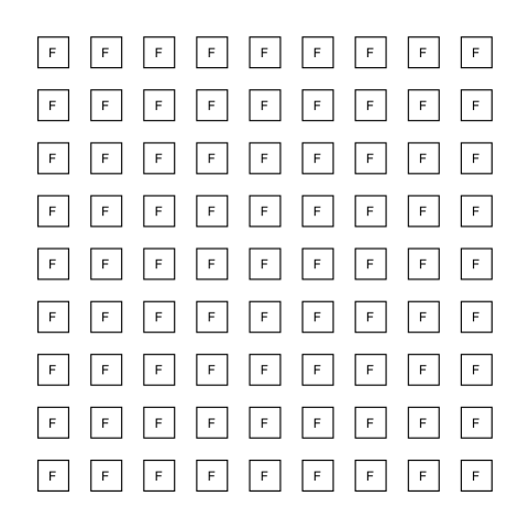
Figure 1: Example of GPU multi-core architecture

Let’s setup our environment and write down our very first CUDA program. For this, we first need to download and install the CUDA Development Tools. For Windows, an installation guide can be found in [NVIDIA, 2020a], for Linux the corresponding installation guide can be found in [NVIDIA, 2020b]. The Linux installation is pretty much straightforward. In contrast, for the Windows installation, we need to further install and link the C++ compiler tools. The following guide summarizes the major stages of setting up a Windows machine:

• Install the CUDA driver.

• Install the CUDA toolkit. Make sure the nvcc compiler is present by typing nvcc –version in the command prompt.

• Make sure Visual Studio (VS) is present at the machine. Furthermore, make sure that the VS module Desktop Development with C++ is installed. In case VS or the VS module is missing, you can always grab the free Visual Studio 2019 community version to be found in [Microsoft, 2021].

• Locate the cl.exe file. For example, if you are using Visual Studio 2019 community version, the default location of the file is similar to C:\ProgramFiles(x86)\MicrosoftVisualStudio\2019\Community\VC\Tools\MSVC\<version>\bin\Hostx64\x64.

• Go to the directory where your CUDA examples are downloaded. In case you want to compile a file with name example.cu, the following command should be typed:

  ⬇

  nvcc -ccbin="C:\Program Files (x86)\Microsoft Visual Studio\2019\Community\VC\Tools\MSVC\<version>\bin\Hostx64\x64" example.cu -o example

  In case no compilation errors occur, the compiled file example.exe should be created in the current directory.

The CUDA platform is designed to work with programming languages such as, but not limited to, C, C++, and Fortran. Throughout this tutorial we are going to use the C language.

Throughout the tutorial, by host we always reference to the CPU, while by device – we reference to the GPU. Every CUDA program could be logically divided into two parts. The first part consists of the host-related code routines, i.e. the source code relevant to the host, while the second part contains the device-related code routines, i.e. the source code relevant to the external device. Assuming that our machine is prepared, let’s compile our first CUDA application.

Figure 2 shows how host and device codes works together.

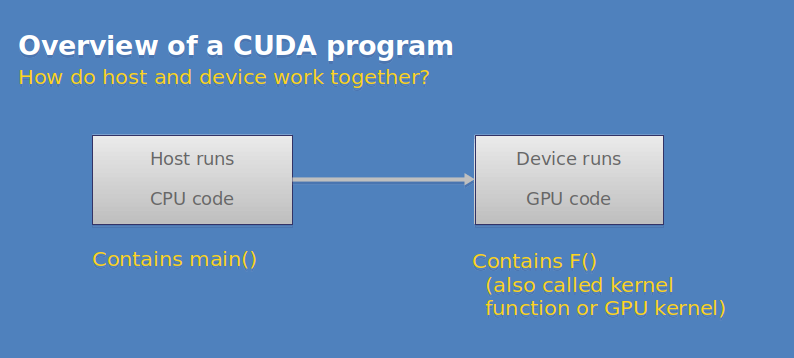
Figure 2: FlowChart: Overview of a CUDA program

2.1 Our first CUDA programs

Listing 1: Our first CUDA program

⬇

1#include <stdio.h>

2

3__global__ void F(){

4 printf("Hello!\n");

5}

6

7int main() {

8 F<<<1,81>>>();

9 cudaDeviceSynchronize();

10 return 0;

11}

The function $F$ (see Listing 1) is a function specific to the device only. By using the declaration __global__ for some function $G$, we announce that $G$ is going to be executed on the device only. In CUDA, we have three different function declarations:

• __global__: functions, that are called from the host and then executed on the device; they are called GPU kernels.

• __device__: functions, that could be called only from the device and executed only on the device.

• __host__: functions, that could be called only from the host and executed only on the host.

However, as we will see later throughout the tutorial, for example in subsection 4.3, in case we need a function to be shared with both the device and the host, we can use both __host__ and __device__ declarations.

The actual initialization of the program starts from the main() function. Then, we call the GPU kernel function $F$ by using this triple-bracket alike syntax: $<<<x,y>>>$, where $x$ defines the number of blocks (will be discussed in Section 4 ), and $y$ defines the number of threads (cores) per block.

Since our hypothetical GPU example (see Figure 1) is based on exactly 81 cores, we launch the kernel by supplying a tuple $<<<1,81>>>$, which means that we are going to launch the $F$ function on all available 81 cores, without dividing them by blocks. Similarly to a C compiling procedure, the compilation is done by using nvcc -o $\{$programName$\}$ $\{$programName$\}$.cu. NVCC is the CUDA compiler driver. Please note, that, as stated in the CUDA documentation, all non-CUDA compilation steps are forwarded to a C++ host compiler that is supported by nvcc.

The cudaDeviceSynchronize() function is a CUDA function, which handles the synchronization of all the threads we have started. Using synchronization is a good practice as it helps to properly print out the messages defined in the $F$ function. We want to emphasize that the kernel calls are asynchronous, which means that the control is returned to the host before the kernel completes. Having this in mind, the application could terminate before the kernel had the opportunity to print out the desired messages.

Let’s compile and run the example. We can see that the message Hello! is printed 81 times in the console. However, in the given situation, we are not able to link a specific row with the corresponding parent GPU core. CUDA provides us with some very important built-in primitives, which can be utilized for thread’s identification numbers. Let’s slightly modify the example to illustrate this (see Listing 2).

Listing 2: CUDA thread identification

⬇

1#include <stdio.h>

2

3__global__ void F(){

4 printf("Hello from thread number %d!\n", threadIdx.x);

5}

6

7int main() {

8 F<<<1,81>>>();

9 cudaDeviceSynchronize();

10 return 0;

11}

The threadIdx.x number returns the unique ID of the thread. The IDs starts from 0, and by considering the current example, up to 80 (inclusive). Now, in case we want to find the squares of all the integer numbers from 0 to 80, we can change a little bit the function F to solve this problem in parallel, benefiting from the GPU architecture (see Listing 3).

Listing 3: CUDA parallel squaring

⬇

1#include <stdio.h>

2

3__global__ void F(){

4 printf("%d squared is: %d! \n", threadIdx.x, threadIdx.x*threadIdx.x);

5}

6

7int main() {

8 F<<<1,81>>>();

9 cudaDeviceSynchronize();

10 return 0;

11}

2.2 Parallel squaring – Part I

What if we want to square a set of numbers, which should be read from the host memory? What is the mechanism of transferring data from the host memory to the device memory? The procedure is similar to the memory allocation in a C language routine. We call the function cudaMalloc((void **)&P, SIZE) which is going to reserve a memory block of size SIZE on the device. The pointer to the reserved block will be saved to the pointer P.

In case we don’t need this memory allocation anymore, we should free it with cudaFree(P). To interchange memory blocks between the host and the device we use the built-in CUDA function cudaMemcpy(). Let’s consider an example which illustrates the usage of these functions (see Listing 4).

Listing 4: CUDA parallel squaring by filling the kernel memory (one-way)

⬇

1#include <stdio.h>

2#define threads 81

3

4__global__ void H(int *d_seeds){

5 int element = d_seeds[threadIdx.x];

6 printf("%d squared is: %d \n", element, element*element);

7}

8

9int main() {

10

11 int seeds[threads];

12

13 for (int j=0; j<threads; ++j)

14 seeds[j] = j;

15

16 int size = sizeof(int);

17 int *d_seeds;

18

19 // allocate memory block on the device

20 cudaMalloc((void **)&d_seeds, size*threads);

21

22 // copy the seeds array to the device memory

23 cudaMemcpy(d_seeds,seeds,size*threads,cudaMemcpyHostToDevice);

24

25 H<<<1,threads>>>(d_seeds);

26 cudaDeviceSynchronize();

27 cudaFree(d_seeds);

28 return 0;

29

30}

Now let us inspect the code line by line. Throughout the process, we are going to depict the memory blocks of the host and the device. As shown in Figure 3, at the beginning both the memory blocks, the host related one (on the left) and the device related one (on the right) are empty.

Figure 3: At the beginning, there is no data on both the CPU and the GPU.

At line 11 of Listing 4 we declare an array of integers called seeds. We will use it as buffer located on the host memory. Then, at lines 13 and 14, we populate the cells in the host memory block with the integer numbers from 0 to 80 (the total number of our threads). At this moment our memory snapshot of the host and the device is given in Figure 4.

Figure 4: The integer array seeds inside the host memory is initialized and filled with values.

At line 17 of Listing 4 we declare an integer pointer called d_seeds, which is going to point to a memory block inside the device (not allocated yet). As shown in Figure 5, there is almost no change in the snapshot of the host and device memory blocks.

Figure 5: The integer pointer d_seeds is created, which is going to point to a block in the device (GPU) memory.

Now, at line 20 of Listing 4 we allocate a memory block on the device (the GPU). The second parameter in the cudaMalloc command defines the total size (in bytes) of the memory block we want to allocate, i.e. size*threads, while the first parameter is the pointer to the allocated memory block. More information regarding the CUDA memory management could be found in [NVIDIA, 2021b]. Figure 6 corresponds to the current memory snapshot of the host and the device. We must take care not to overwrite the value of d_seeds. Otherwise the address of the allocated device memory block is lost. Therefore, we highlighted this interconnection as a red thick line.

Figure 6: Using cudaMalloc() a memory block on the GPU is allocated to contain 81 integer cells. d_seeds points to the exact memory address of this block inside the GPU memory.

To proceed, we need to transfer the host memory block to the device memory block. For this purpose, we are going to use the aforementioned cudaMemcpy function. Line 23 of Listing 4 copies the contents from the host memory block seeds to the device memory block d_seeds. The total size of data to be transferred is defined via size*threads. The current snapshot of host and device memory blocks is given in Figure 7. The gray dotted line highlights the direction of the transferred data. In this case, since we call the cudaMemcpy routine with the “cudaMemcpyHostToDevice” option, the dotted arrow is pointing to the device memory block.

Figure 7: cudaMemcpy() transfers the data from the host seeds array to the device d_seeds array.

Line 25 of Listing 4 calls the device function H 81 times in a loop from 1 to 81). So a total of 81 threads are defined, each with an instance of H.

Before launching the kernel function H all required data should have been transmitted to the GPU memory. Each thread from the GPU device is going to read the corresponding memory cell from the device memory block, which is defined as the global memory. More details regarding the CUDA memory model are presented in Section 5. Then, the result is printed in the console output. The current snapshot is shown in Figure 8.

Figure 8: After all information has been transmitted to the GPU memory, each GPU thread launches it’s own instance the kernel function H.

Finally, cudaFree() frees the allocated device memory block (line 27 of Listing 4). The final snapshot of host and device is given in Figure 9. Now the variable d_seeds points to an un-allocated memory block in the device, which is depicted by a dotted red line.

Figure 9: Finally, when all of the 81 instances of H are finished, the memory block allocated on the device is freed.

Launching the kernel H activates all the defined threads. However, we should be very carefully in writing the kernel routines. For example, fragments of memory blocks, to which two or more threads have unintentional write access is an undesirable behavior in our program. Let’s take two different threads $t_{1}$ and $t_{2}$, and some bytes located on the device memory block denoted as $B_{x}$, to which both threads $t_{1}$ and $t_{2}$ have write access. While the kernel routine $t_{1}$ writes to $B_{x}$ the value $v_{1}$, $t_{2}$ writes the value $v_{2}$ to $B_{x}$. In this scenario, and when the kernel routines are finalized, we can only speculate what is the final value of $B_{x}$ – $v_{1}$ or $v_{2}$. Having this in mind, we should always check for possible thread interference or deadlocks.

The threads on the device and the used GPU memory are visualized in Figure 10. Since each thread has a unique thread id (via the call in Line 25 of Listing 4), each thread, labeled with an id number, is visualized as a distinct color. Above the labeled threads, an illustrative example of the GPU global memory is shown. Starting from left to right, each color stripe corresponds to the thread id sharing the same color. In this specific example, we have organized the corresponding color map from lower id numbers to higher ones, i.e. thread id 0 is at the left-most positioned stripe inside the global device memory, while thread id 80 corresponds to the final right-most stripe inside the global memory. Each stripe is strictly related to the thread block sharing the same color.

Figure 10: Visualization of the GPU global memory as a multi-color rectangle (to be found above the thread matrix). Each GPU thread and each stripe is depicted with a distinct color.

In Listing 5 an example output on the host terminal is given. Some lines of the output are omitted. Since each thread is independent from the others and the order of thread completion is hard to predict, the results could be reported back in a scrambled way.

Listing 5: Example output of Listing 4

⬇

console:nvcc 4Hello.cu -o hello

console:./hello

64 squared is: 4096

65 squared is: 4225

66 squared is: 4356

...omitted...

78 squared is: 6084

79 squared is: 6241

80 squared is: 6400

0 squared is: 0

1 squared is: 1

2 squared is: 4

...omitted...

61 squared is: 3721

62 squared is: 3844

63 squared is: 3969

console:

2.3 Parallel squaring – Part II

Now, let’s try another strategy – instead of printing out the squared numbers by the kernel threads, we can copy the results calculated in the device memory block back to the given host memory block (so the host prints the results). In fact, calling the printing function inside the kernel is not a common routine and should be avoided. The modified program is shown in Listing 6.

Listing 6: CUDA parallel squaring with filling and reading the kernel memory from the host (two-way)

⬇

1#include <stdio.h>

2#define threads 81

3

4__global__ void K(int *d_seeds){

5 d_seeds[threadIdx.x]=d_seeds[threadIdx.x]*d_seeds[threadIdx.x];

6}

7

8int main() {

9

10 int seeds[threads];

11

12 for (int j=0; j<threads; ++j)

13 seeds[j] = j;

14

15 int size = sizeof(int);

16 int *d_seeds;

17

18 // allocate memory block on the device

19 cudaMalloc((void **)&d_seeds, size*threads);

20

21 // copy the seeds array to the device memory

22 cudaMemcpy(d_seeds,seeds,size*threads,cudaMemcpyHostToDevice);

23

24 K<<<1,threads>>>(d_seeds);

25 cudaDeviceSynchronize();

26

27 // copy the results array back to the host memory

28 cudaMemcpy(seeds,d_seeds,size*threads,cudaMemcpyDeviceToHost);

29 cudaFree(d_seeds);

30

31 for (int j=0; j<threads; ++j)

32 printf("Cell %d is equal to: %d\n", j, seeds[j]);

33

34 return 0;

35

36}

At line 5 in Listing 6, inside the newly defined kernel function K, we write the result of squaring the number back to the d_seeds array. The main function remains almost the same as in the previous example. The only difference is that, this time (see line 28) we transfer the results back to the host memory, i.e. we copy the data pointed by d_seeds to seeds. The fourth argument of the cudaMemcpy function is cudaMemcpyDeviceToHost. Finally, as shown at lines 31 and 32, the results are printed out from the outside of the device. As a summary, the snapshot of the host and the device during these operations (line 28 from Listing 6) is given in Figure 11. The gray dotted line highlights the direction of the transferred data. In this case, since we call the cudaMemcpy routine with the “cudaMemcpyHostToHost” option, the dotted arrow is pointing to the host memory block.

Figure 11: cudaMemcpy() transfers data back from the device memory array to the host seeds array.

We have developed a handy pen-and-paper method to proactively design and architect a GPU implementation. Now, we have all the necessary tools to complete our first project – a full GPU-based automatic cryptanalysis tool for messages encrypted by a monoalphabetic substitution cipher.

3 GPU cryptanalysis

In this section, we are going to launch an automatic GPU-based cryptanalysis on English messages encrypted by a substitution cipher. However, the method is universal for any language, as long as you possess the necessary statistics.

For example, in this section, we are going to exploit the partially-predictable structure of the English language by using bigrams.

3.1 Frequency analysis

Let’s assume that we have a single file describing the properties of the English language bigrams. At each row of this file a single bigram with its corresponding score value is given. Since we have a total of 26 letters in the English alphabet we have a total of $26*26=676$ distinct rows (bigrams from AA to ZZ). Each score for a given bigram reflects the likelihood of this specific bigram to participate in an authentic English text. In short, the higher the overall score, the closer to a grammatically correct English the text is.

For example, one of the most frequently seen bigrams in English texts are th, he, in, er, an, re, es, on and st (ordered by their magnitude of appearance). The likelihood of a given bigram to participate in some English text is calculated by analyzing big databases of English corpus.

Imagine we have a huge digital library of English books. Then, by ignoring all the special symbols and by treating all the letters as lowered-cased ones, we can iterate over all the parsed texts and count the total number of appearances of distinct bigrams. For example, let’s analyze the amusing quote linked to Margaret Mead:

Always remember that you are absolutely unique.
Just like everyone else…

Now, we parse the text to clean it up from special symbols and to further lowercase all the letters:

alwaysrememberthatyouareabsolutelyuniquejustlikeeveryoneelse

We ended up with a string of length 60, i.e. it consists of 59 bigrams we need to analyze:

$$\text{al},\text{lw},\text{wa},\cdots,\text{ls},\text{se}$$

This resulted in the following statistics: ’al’: 1, ’lw’: 1, ’wa’: 1, ’ay’: 1, ’ys’: 1, ’sr’: 1, ’re’: 2, ’em’: 2, ’me’: 1, ’mb’: 1, ’be’: 1, ’er’: 2, ’rt’: 1, ’th’: 1, ’ha’: 1, ’at’: 1, ’ty’: 1, ’yo’: 2, ’ou’: 1, ’ua’: 1, ’ar’: 1, ’ea’: 1, ’ab’: 1, ’bs’: 1, ’so’: 1, ’ol’: 1, ’lu’: 1, ’ut’: 1, ’te’: 1, ’el’: 2, ’ly’: 1, ’yu’: 1, ’un’: 1, ’ni’: 1, ’iq’: 1, ’qu’: 1, ’ue’: 1, ’ej’: 1, ’ju’: 1, ’us’: 1, ’st’: 1, ’tl’: 1, ’li’: 1, ’ik’: 1, ’ke’: 1, ’ee’: 2, ’ev’: 1, ’ve’: 1, ’ry’: 1, ’on’: 1, ’ne’: 1, ’ls’: 1, ’se’: 1.

So, the probability of some random bigram to be ve or el is respectively $\frac{1}{59}$ or $\frac{2}{59}$. However, this is far from adequate statistics – we have used a tiny negligible fragment of English corpus.

Let’s continue with the construction of our main tool. Since working with strings is slow, we can create a map between bigrams and some integer array of length 676, which is going to hold down all the bigram score values.

Let’s define the English alphabet as $\Omega=\{A,B,C,\cdots,Z\}$. We map each consequent alphabet letter from $\Omega$ to an integer value from 0 to 25, i.e.

$$A\rightarrow 0,B\rightarrow 1,C\rightarrow 2,\cdots,Z\rightarrow 25.$$

Let’s store the score values of each of the bigrams in the array $L$ of length ${|\Omega|}^{2}=26^{2}=676$. For each of the bigrams $\overline{\mu\nu}$ we compute it’s index in $L$ as $26\mu+\nu$.

For example, the score of bigram $\overline{AB}$ is mapped to the index $26*0+1=1$ of $L$, while the score of bigram $\overline{CA}$ is mapped to the index $26*2+0=52$ of $L$. The score of the last bigram over $\Omega$, i.e. $\overline{ZZ}$, is mapped to the index $26*25+25=675$ of $L$.

Now, our first task is to read and parse the file with all the English bigrams and their corresponding score values. Then, we need to organize and map the score values into an array following the aforementioned mapping. Finally, we are going to transfer the created mapped array to the device global memory, making the array accessible within each GPU thread. The code fragment is given in Listing 7.

Listing 7: Helper function to read and parse from bigram collection file

⬇

1// a host function to extract and map

2// all the bigrams from a given file

3__host__ void extractBigrams(unsigned long long int *scores) {

4 FILE* bigramsFile = fopen("bigramParsed", "r");

5 while(1){

6 char tempBigram[2];

7 unsigned long long int tempBigramScore = 0;

8 if (fscanf(bigramsFile, "%s %llu", tempBigram, &tempBigramScore) < 2)

9 { break; }

10 scores[(tempBigram[0]-’a’)*26 + tempBigram[1]-’a’] = tempBigramScore;

11 }

12 fclose(bigramsFile);

13}

As shown in the previous source code fragment, we named the bigram collection file as bigramParsed (line 4). Then, by reading the file line by line, we repeatedly extract each bigram and then compute the corresponding score (see line 8). We recall that the fscanf function reads data from the current position of the specified stream into the locations that are given by the entries in the argument-list. The actual mapping is done at line 10. To achieve that, we subtract the ascii value of a from each letter from the bigram, so:

• a is mapped to 0

• b is mapped to 1

• $\cdots$

• z is mapped to 25

Having this in mind, the helper function is adequate to low-cased bigrams collection related files only. If you want to use another bigram format then a further modification of the function logic is needed.

Finally, we save all the scores to an unsigned long long int array named scores. The main function of our GPU cryptanalysis tool is given in listing 8. Take a brief look, but don’t try to grasp all the details and “magic” constants yet. A detailed explanation accompanied by helpful comments is given right after the source code fragment.

Listing 8: The main function of the CUDA mas cryptanalysis project

⬇

1int main() {

2

3 srand(time(0));

4 int totalBigrams = 676;

5 int threads = 325;

6 char encrypted[] = <omitted>;

7 int encryptedLen = strlen(encrypted);

8 int encryptedMap[encryptedLen];

9

10 unsigned long long int results[threads];

11

12 // we map the encrypted message to integers

13 for (int j=0; j<encryptedLen; ++j)

14 encryptedMap[j] = encrypted[j] - ’a’;

15

16 unsigned long long int scores[totalBigrams];

17 extractBigrams(scores);

18

19 int size = sizeof(unsigned long long int);

20 unsigned long long int *d_scores;

21 unsigned long long int *d_results;

22 int *d_encrypted;

23

24 // allocate memory blocks on the device

25 cudaMalloc((void **)&d_scores, size*totalBigrams);

26 cudaMalloc((void **)&d_results, size*threads);

27 cudaMalloc((void **)&d_encrypted, sizeof(int)*encryptedLen);

28

29 // copy the scores array to the device memory (only once)

30 cudaMemcpy(d_scores, scores, size*totalBigrams, cudaMemcpyHostToDevice);

31

32 int leftLetter = 0;

33 int rightLetter = 0;

34 int tempMaxIndex = 0;

35 int tempMaxLeft = 0;

36 int tempMaxRight = 0;

37 unsigned long long int maxScore = 0;

38

39 for (int j=0; j<500; ++j) {

40

41 // pick two random distinct letters; we make sure they do exists in the encrypted text

42 leftLetter = encrypted[rand() % encryptedLen] - ’a’;

43 rightLetter = leftLetter;

44 while (rightLetter == leftLetter)

45 rightLetter = encrypted[rand() % encryptedLen] - ’a’;

46

47 // copy the encrypted msg array to the device memory (after each climbing)

48 cudaMemcpy(d_encrypted, encryptedMap, sizeof(int)*encryptedLen, cudaMemcpyHostToDevice);

49

50 K<<<1,threads>>>(d_scores, d_encrypted, encryptedLen, leftLetter, rightLetter, d_results);

51 cudaDeviceSynchronize();

52

53 // copy the results array back to the host memory

54 cudaMemcpy(results, d_results, size*threads, cudaMemcpyDeviceToHost);

55

56 tempMaxIndex = getMaxElement(results, threads);

57

58 if (results[tempMaxIndex] > maxScore) {

59 maxScore = results[tempMaxIndex];

60 tempMaxLeft = 0;

61 tempMaxRight = 0;

62 translateIndexToLetters(tempMaxIndex, &tempMaxLeft, &tempMaxRight);

63 climb(encryptedMap, encryptedLen, leftLetter, tempMaxLeft, rightLetter, tempMaxRight);

64 printf("%d %llu\n", tempMaxIndex, results[tempMaxIndex]);

65 printf("%d %d %d %d\n", tempMaxLeft, tempMaxRight, leftLetter, rightLetter);

66 demap(encryptedMap, encryptedLen);

67

68 }

69 }

70

71 // we free the allocated device memory

72 cudaFree(d_scores);

73 cudaFree(d_encrypted);

74 cudaFree(d_results);

75

76 return 0;

77}

Line 3 initializes the seed of the prng, which is going to be repeatedly utilized throughout the main function core routine. There are a total of $26^{2}=676$ bigrams over the English language (line 4). The encrypted message is defined as a string with name encrypted (line 6). We further take its length (line 7), and make a declaration of another array of integers named encryptedMap, of the same length as the encrypted message itself (line 8).

3.2 On the multi-threaded hill climbing design

Now let’s pause for a while. Since we want to utilize the multi-core capabilities of the GPU, we are going to perform a multi-threaded hill-climbing method to automatically decrypt a given message encrypted by mas cipher. Hill climbing is a mathematical optimization technique and an iterative algorithm that starts with an arbitrary solution to a problem, then attempts to find a better solution by making an incremental change to the solution. If the change produces a better solution, another incremental change is made to the new solution, and so on until no further improvements can be found. More details can be found in [Lasry, 2018].

Now, for simplicity, let’s denote the encrypted message as $E$, which was constructed over some alphabet $\Omega$.

Let’s denote the key of the mas cipher as $K$. We can decompose $K$ to 26 single substitutions, i.e.:

$$a\rightarrow\zeta_{0}$$

$$b\rightarrow\zeta_{1}$$

$$\cdots$$

$$z\rightarrow\zeta_{25,}$$

where $\zeta_{i}\in\Omega$ and $\forall i,j\implies\zeta_{i}\neq\zeta_{j}$. A normal hill-climbing approach to recover an unknown key of such encryption scheme can be summarized with the following steps:

1. Generate two random letters $\psi_{1}$ and $\psi_{2}$ over the alphabet $\Omega$.

2. Given an encrypted message $E$, interchange all the letters $\psi_{1}$ with $\psi_{2}$. Let’s denote the resulted message as $E^{\prime}$.

3. By using bigrams (or any other statistics) compare the scores of $E$ and $E^{\prime}$. If $E^{\prime}$ is a better candidate than $E$, we overwrite $E$ with $E^{\prime}$.

4. Repeat until some threshold value is reached.

Since we want to benefit from the multi-core capabilities of the GPU, we can tweak and modify the normal hill climbing algorithm with the following multi-threaded hill variant:

1. Generate two random distinct letters $\psi_{l}$ and $\psi_{r}$ over the alphabet $\Omega$. Given an encrypted message $E$, we make sure that both $\psi_{l},\psi_{r}\in E$.

2. Launch the kernel function in such a way, that every distinct thread corresponds to a unique unordered pair of distinct letters $\delta_{l}$ and $\delta_{r}$ over the alphabet $\Omega$. Let us define such mapping as $\Upsilon$.

   Example: Let’s say we have an encrypted message $E$ over some reduced alphabet consisting of the letters a, b and c only. Since the reduced alphabet consists of 3 letters, the total count of unique pairs of distinct letters $\delta_{l}$ and $\delta_{r}$ over $\Omega$ is $\frac{3*2}{2}=3$. Indeed, we have the following possible set of ordered pairs $\delta_{l}$ and $\delta_{r}$:

   $$\left(\delta_{l},\delta_{r}\right)=\left\{\left(a,b\right),\left(a,c\right),\left(b,a\right),\left(b,c\right),\left(c,a\right),\left(c,b\right)\right\}$$

   .. which is reduced to the following set of unordered pairs $\delta_{l}$ and $\delta_{r}$:

   $$\left(\delta_{l},\delta_{r}\right)=\left\{\left(a,b\right),\left(a,c\right),\left(b,c\right)\right\}$$

   Having this in mind, we need to utilize a total number of 3 GPU threads. Let’s denote them as $t_{1},t_{2}$ and $t_{3}$. A possible mapping $\Upsilon_{1}$ could be:

   $$\Upsilon_{1}:t_{1}\rightarrow(b,c);t_{2}\rightarrow(a,c);t_{3}\rightarrow(a,b)$$

   This is a valid mapping, since each thread is mapped to a distinct pair and there is a total number of 3 mappings.

3. Given an encrypted message $E$, each thread should interchange $\psi_{l}$ with $\delta_{l}$, as well as $\psi_{r}$ with $\delta_{r}$. However, to guarantee that the order of the interchanges is irrelevant, we make sure that they take place if and only if $\psi_{l}\neq\delta_{r}$ and $\psi_{r}\neq\delta_{l}$. Let’s denote the resulted message as $E^{\prime}$.

4. By using bigrams, each distinct thread calculates the corresponding score of $E^{\prime}$ denoted by $F(E^{\prime})$. Then, the score $F(E^{\prime})$ is further saved to the corresponding thread memory cell. When all the threads are ready and synchronized, we transfer back all the scores to the host.

5. We analyze all the scores and pick up the best yielded score. Let’s denote the best score on index $i$ as $F(E^{{}^{\prime}}_{i})$. If $E^{{}^{\prime}}_{i}$ possesses a better score than $E$, we overwrite $E$ with $E^{\prime}_{i}$.

   We should emphasize that currently we have $F(E^{{}^{\prime}}_{i})$, not $E^{{}^{\prime}}_{i}$ itself. However, by taking the index of the best yielded score, i.e. $i$, we can reconstruct the actual value of $E^{{}^{\prime}}_{i}$. We can easily achieve that by applying the inverse mapping $\Upsilon^{-1}$ on thread number $i$.

   Example: We use the same scenario as in step 2. We have the following setup before launching the GPU threads on the encrypted message $E$:

   $$\Upsilon_{1}:t_{1}\rightarrow(b,c);t_{2}\rightarrow(a,c);t_{3}\rightarrow(a,b)$$

   The letters $\psi_{l},\psi_{r}\in E$ are chosen pseudo-randomly. By applying the interchanges described above, a given text $E_{i}$ is computed by the corresponding thread $t_{i}$, i.e. $t_{1}\rightarrow E_{1},t_{2}\rightarrow E_{2},$ and $t_{3}\rightarrow E_{3}$. Then, the concatenated values of the scores of $E_{i}$ are transferred back to the host. Let’s store these values in the array $F(E_{1})|F(E_{2})|F(E_{3})$. Now, suppose that $F(E_{2})$ is the best among all the scores. We further recall that the host doesn’t have the $E_{2}$ text itself at the moment. However, we know the position of $F(E_{2})$, i.e. $2$, which corresponds to the index of the thread that yielded this score, e.g. $t_{2}$. By using the inversion mapping of $\Upsilon_{1}$:

   $$\Upsilon_{1}^{-1}:(b,c)\rightarrow t_{1};(a,c)\rightarrow t_{2};(a,b)\rightarrow t_{3},$$

   we can trace-back the operation on $E$, which yielded $E_{2}$ and, therefore, fully recover it.

6. We repeat until some threshold value is reached. This value usually depends on the size of the set of the possible initial choices (in our implementation we have two choices – $\psi_{l}$ and $\psi_{r}$).

One could ask – ”What is the reason to introduce step 1? Why don’t we just try all the possible unordered pairs $(\delta_{i},\delta_{j})$ inside the GPU?”. Well, such strategy would benefit from the multi-core architecture of the GPU as well. However, there is one major drawback – it is deterministic. To illustrate that, let’s start from some encrypted message $E$ over some alphabet $\Omega$, s.t. $|\Omega|=n$. We transfer $E$ to the GPU, together with all the necessary data to evaluate the generated candidates. We skip step 1 and we do not generate two letters $\psi_{i}$ and $\psi_{j}$, s.t. $\psi_{i},\psi_{j}\in\Omega$. Each GPU thread corresponds to a given transposition of letters in $E$. Without loss of generality, we can represent the thread mapping in lexicographical order, i.e.:

$$\Upsilon:$$

$$t_{1}\rightarrow(\delta_{1},\delta_{2})$$

$$t_{2}\rightarrow(\delta_{1},\delta_{3})$$

$$\cdots$$

$$t_{x}\rightarrow(\delta_{i},\delta_{j}),i<j$$

$$\cdots$$

$$t_{\frac{n(n-1)}{2}}\rightarrow(\delta_{n-1},\delta_{n})$$

Now, let’s denote the generated candidate from a given thread $t_{i}$ as $E_{i}$. Furthermore, let’s denote the score results of $E_{i}$ under some evaluating function $F$ as $F(E_{i})$. For simplicity, we choose $F$ in such a way, that

$$\forall i,j\in\left[1,T\right],i\neq j:F(E_{i})\neq F(E_{j}).$$

with $T=\frac{n(n-1)}{2}$. Then, we have the following composition:

$$\Upsilon\circ F:$$

$$t_{1}\rightarrow(\delta_{1},\delta_{2})\rightarrow E_{1}\rightarrow F(E_{1})$$

$$t_{2}\rightarrow(\delta_{1},\delta_{3})\rightarrow E_{2}\rightarrow F(E_{2})$$

$$\cdots$$

$$t_{x}\rightarrow(\delta_{i},\delta_{j})\rightarrow E_{x}\rightarrow F(E_{x})$$

$$\cdots$$

$$t_{T}\rightarrow(\delta_{n-1},\delta_{n})\rightarrow E_{T}\rightarrow F(E_{T})$$

Then, we collect all the resulting scores and choose the best candidate $E_{m}$, s.t.

$$\forall i\in\left[1,T\right],i\neq m:F(E_{i})<F(E_{m}).$$

Let’s denote as $M_{1}$ the value of the maximum achieved score, i.e.

$$M_{1}=\max_{i=1}^{T}{F(E_{i})}=F(E_{m})$$

Now, if we restart the process from the beginning, the best yielded score will be exactly the same value, i.e. $M_{1}$. However, if we do not restart the process the optimization process will proceed as usual – since $F(E_{m})$ can be found at the position $m$, then the thread $m$ yielded this score, i.e. $t_{m}$. Hence, we interchange the current message $E$ with the reconstructed better candidate $E_{m}$. Then, we repeat the procedure until we have reached a local maximum candidate $E_{max}$. Let’s denote the best score yielded on iteration $i$ as $M_{i}$. The history of our best yielded scores during the optimization process could be summarized as follows:

$$M_{1},M_{2},\cdots,M_{k-1},M_{k},\text{NA}$$

where NA is the abbreviation of ”not available”, denoting the absence of a better score after the k-th iteration step.

We can generalize our previous observation, by stating that the restart of the optimization process from a given encrypted message $E_{x}$, which corresponds to, for example, a score $M_{x}$, and applying only one iteration, will lead to the best yielded score $M_{x+1}$. Therefore, if we restart the process from the beginning, we will reach $M_{1}$, then $M_{2}$, $\cdots$, then $M_{k}$, to travel exactly the same optimization path, and to reach exactly the same final local optimum. In this scenario, having a complete deterministic metaheuristic, we define $M_{k}$ as the attractor of $M_{1}$.

3.3 Implementation

Now, in the context of our current problem, we can define the bijective mapping $\Upsilon$ as a lexicographical order mapping. Since we have a total of 26 letters, without considering the interchanging restriction introduced in step 3, we need a total of ${26\choose 2}=325$ threads (see line 5 of the main function source code).

We save all the scores reported back from the device threads into the results array (defined at line 10). A regular mapping from ASCII to integer indexes is performed on the encrypted text as well (lines 12-14). The current snapshot of the memory blocks of the host and the device is given in Figure 12.

Figure 12: First steps of initializing the algorithm presented in Listing 8.

At the beginning, we read the encrypted message from a given file and save it in the character array encrypted. Then, we translate the character message to an integer one by using the integer array encryptedMap. We continue by creating an array results which is going to keep the scores yielded by each GPU thread. Finally, we populate an array named scores with the bigram scores we have prepared (lines 16 and 17 in Listing 8).

We are ready to prepare and allocate all the necessary memory blocks inside the device global memory (lines 19-30). The memory block snapshot is depicted in Figure 13.

Figure 13: Creating the GPU memory blocks we are going to use.

First, we create the necessary pointers. Then, the required space is allocated on the GPU global memory (lines 19-27 in Listing 8). For simplicity, we denote the variable type unsigned long long int with ulli.

Then, the bigram scores are transferred from the host to the device. After that, we enter the for block. The snapshot of the memory blocks of the host and the device, right before entering the for cycle, is given in Figure 14.

Figure 14: The GPU transfer of the bigram scores and launching the FOR cycle.

We transfer to the GPU the bigram scores (line 30 in Listing 8). This is done just once. Next, we enter a for cycle, which is iterated 500 times.

Starting from line 39 to line 69, we initiate the actual multi-threaded hill climbing instance. We define a reasonable number of iterations value of 500 (at line 39). By reasonable, we are emphasizing on the negligible probability of missing a better candidate, if such exists.

First, we generate two random distinct letters $\psi_{l}$ and $\psi_{r}$ over the English alphabet, which are to be seen at least once in the encrypted text (see lines 41-45). We further transfer the encrypted message to the device – recall that the message is not static and is always replaced in the cases when better candidate messages are found. By completing the aforementioned routines, we are ready to launch the kernel K. As soon as the kernel is activated, each thread applies the corresponding (unique) interchange $(\psi_{l}\rightarrow\delta_{l},\psi_{r}\rightarrow\delta_{r})$ and further calculates the score of the modified text. Then, the score is saved to the dedicated cell inside the threads array. Completing all the steps described in this paragraph will yield the memory block snapshot of the host and the device shown in Figure 15.

Figure 15: Launching kernel K.

By using the host (CPU) prng we generate two distinct letters leftLetter and rightLetter and transfer the encrypted text to the device (line 47 in Listing 8). We launch the kernel K. Once the routine is finished, the results are populated inside the d_results array on the GPU.

Then, we transfer back the results (lines 48-54), to further analyze them and extract the best score. The extraction of the best score is given by the following helper function getMaxElement (see Listing 9):

Listing 9: The getMaxElement helper function

⬇

1// a helper function to return the maximum element

2__host__ int getMaxElement(unsigned long long int *scores, int length) {

3 unsigned long long int tempMaxScore = 0;

4 int tempIndex = 0;

5 for (int j=0; j<length; ++j) {

6 if (scores[j] > tempMaxScore) {

7 tempIndex = j;

8 tempMaxScore = scores[j];

9 }

10 }

11 return tempIndex;

12}

If better candidate $E^{\prime}_{i}$ is found, we accept it and update the current state (lines 58-69). Several helper functions are called inside this routine. In order to recover the candidate $E^{\prime}_{i}$, as we have previously discussed, we need to calculate the $\Upsilon^{-1}$ bijective mapping. This is done by the helper function translateIndexToLetters (see Listing 10):

Listing 10: The translateIndexToLetters helper function

⬇

1// translate a given index to a map of pair of distinct letters

2__host__ void translateIndexToLetters(int index, int* left, int* right) {

3

4 int tempLeft = 0;

5 int tempRight = tempLeft+1;

6

7 while (index > 0) {

8 tempRight += 1;

9 index -= 1;

10 if (tempRight == 26) {

11 tempLeft += 1;

12 tempRight = tempLeft + 1;

13 }

14 }

15

16 *left = tempLeft;

17 *right = tempRight;

18}

Next, we continue with the main function routines. We accept the better candidate by calling the helper function climb (see Listing 11):

Listing 11: The climb helper function

⬇

1// interchange left with maxLeft and right with maxRight

2__host__ void climb(int* encrMap, int length, int left, int maxLeft, int right, int maxRight) {

3 for (int j=0; j<length; ++j) {

4 if (encrMap[j] == left)

5 encrMap[j] = maxLeft;

6 else if (encrMap[j] == maxLeft)

7 encrMap[j] = left;

8 else if (encrMap[j] == right)

9 encrMap[j] = maxRight;

10 else if (encrMap[j] == maxRight)

11 encrMap[j] = right;

12 }

13}

In case a better candidate is found, we print out some details about the candidate (lines 64 and 65), as well as the current state of the message to be decrypted (line 66). This is done by the helper function demap (see Listing 12), which should not be mistaken with the bijective mapping $\Upsilon$:

Listing 12: The demap helper function

⬇

1// demap and print a given array of integer letters

2__host__ void demap(int* encrMap, int length) {

3 for (int j=0; j<length; ++j) {

4 printf("%c", encrMap[j] + ’a’);

5 }

6 printf("\n");

7}

Figure 16 summarizes the current snapshot of memory blocks of the host and the device.

Figure 16: The results transfer from the device (the GPU) to the host (CPU).

We transfer the results from the device (the GPU) to the host (CPU) (line 54 in Listing 8), to further analyze them and pick the best candidate. We further update the current text by using the helper function climb. Once this is done, we step into the next iteration of for cycle.

The final construction of the kernel and the complete version of the program is given in Listing 13. For a better overview some sections are omitted. The full code, including a real example to decrypt, is given in Listing 14.

Listing 13: The complete GPU monoalphabetic-substitution solver.

⬇

1#include <stdio.h>

2#include <stdlib.h>

3#include <string.h>

4#include <time.h>

5

6__host__ void extractBigrams() { /* omitted */ }

7__host__ int getMaxElement() { /* omitted */ }

8__host__ void translateIndexToLetters() { /* omitted */ }

9__host__ void climb() { /* omitted */ }

10__host__ void demap() { /* omitted */ }

11

12__global__ void K(unsigned long long int *d_scores, int *d_encrypted, int encryptedLen, int leftLetter, int rightLetter, unsigned long long int *d_results){

13 int tempLeft = 0;

14 int tempRight = tempLeft+1;

15 int remainder = threadIdx.x;

16

17 while (remainder > 0) {

18 tempRight += 1;

19 remainder -= 1;

20 if (tempRight == 26) {

21 tempLeft += 1;

22 tempRight = tempLeft + 1;

23 }

24 }

25

26 unsigned long long int total = 0;

27 int detectorLeft = 0;

28 int detectorRight = 0;

29 for (int j=0; j<encryptedLen-1; ++j)

30 {

31 detectorLeft = d_encrypted[j];

32 detectorRight = d_encrypted[j+1];

33 if (d_encrypted[j] == leftLetter)

34 detectorLeft = tempLeft;

35 else if (d_encrypted[j] == tempLeft)

36 detectorLeft = leftLetter;

37 else if (d_encrypted[j] == rightLetter)

38 detectorLeft = tempRight;

39 else if (d_encrypted[j] == tempRight)

40 detectorLeft = rightLetter;

41 else if (d_encrypted[j+1] == leftLetter)

42 detectorRight = tempLeft;

43 else if (d_encrypted[j+1] == tempLeft)

44 detectorRight = leftLetter;

45 else if (d_encrypted[j+1] == rightLetter)

46 detectorRight = tempRight;

47 else if (d_encrypted[j+1] == tempRight)

48 detectorRight = rightLetter;

49 total += d_scores[detectorLeft*26 + detectorRight];

50 }

51 d_results[threadIdx.x] = total;

52 if ((tempLeft == rightLetter) || (tempRight == leftLetter))

53 d_results[threadIdx.x] = 0;

54}

55

56int main() { /* omitted */ }

Lines 13-24 (to be found inside the kernel definition) are mapping each thread number to specific unique pair of letters by using the bijective mapping $\Upsilon$. Then, each thread applies the corresponding interchange to calculate the score of the newly created candidate (lines 26-51). Furthermore, we make sure the restriction we have introduced in step 3 of the multi-threaded hill climbing variant is valid (lines 52 and 53). If we happen to be in a thread, where this restriction is not valid, we give the candidate the lowest possible score of 0.

It should be emphasized that running a single instance of the final program doesn’t guarantee a successful decryption of the encrypted text. In fact, it’s highly unlikely that the plaintext is found immediately after the first try. Due to the high number of possible keys in the key search space, i.e. $26!$, the multi-threaded hill-climbing algorithm can easily stuck in some local maximum. A helpful illustration is given in Figure 17.

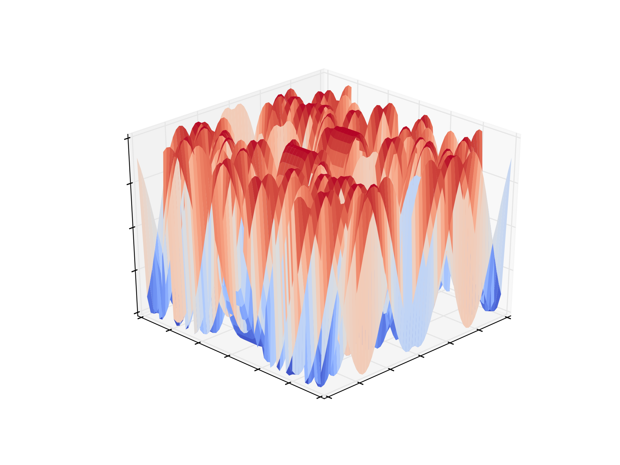
Figure 17: Example of metaheuristics topology. The depicted topology serves as an illustration only. This specific example is generated by using the score (fitness) equation $z=\sin{\left(|x|+y^{8}\right)}$

The cold areas (nuances of blue) corresponds to candidates with low score values, while the hot areas (nuances of red) corresponds to candidates with higher score values. The algorithm usually starts from some random blue position and repetitively makes its way to the top. However, the finally reached peak only guarantee that there is no neighbor with a better score value than the peak itself – it doesn’t guarantee that it is the highest peak possible. As you can see in Figure 17 we have a rich set of peaks, but in most real-world application, there is only one peak we are interested in. In literature, each peak is defined as a local maximum, while the highest peak is declared as the global maximum.

If we are stuck in a local maximum, we should either try to escape from this peak (by actions which worsen the objective function value), or to reinitialize the optimization problem from the beginning. Having this in mind, we should reinitialize the GPU program several times and to collect all the reached peaks. Hopefully, one of them will be the global maximum.

As an exercise, instead of manually reinitialize the program until the desired peak is reached, implement another loop wrapper of the main loop, to automatically reinitialize the multi-thread hill climbing algorithm.

Few words should be mentioned regarding some difficulties you could experience during the compilation of a given CUDA source. More precisely, in those cases when you are using Windows OS as a host, the Microsoft provided compilers and linkers do not support the C programming language standard C99 (ISO/IEC 9899:1999). There are some noticeable differences between C99 and newer standards. More detailed information could be found in [OpenSTD, 2021].

One common issue which arises during the process of migrating a C99 complaint program to a newer standard is the restriction on declaring static arrays with non-constant lengths. Having this in mind, all the source codes to be found in this tutorial are attuned to be C99, C11 and C17 compatible.

One last thing before delving into our first real problem task. As we have already mentioned, all non-CUDA compilation steps are forwarded to a C++ host compiler. If you want to send some addition options to the compiler, like optimization flags, the standard that should be taken under consideration, or anything else, the -Xcompiler switch could be used. More detailed information could be found in the CUDA Toolkit Documentation [NVIDIA, 2021c].

In Listing 14 the complete source code of Listing 13 is given. This is our first practical usage of the tools we have created so far. The lines 8-11 introduce the flexibility of the provided example, so to be easily compiled on C99, C11 or C17 programming language standards. The source code is to be compiled by nvcc. Can you recover the encrypted message and find the original book from which the plaintext was extracted? Please note: it is highly unlikely that you will be able to successfully decrypt the encrypted message from the first try. A little bit more tries are required for reaching the real solution. In most of the times you will be stuck in some local maximum having a gibberish-looking text. Just keep trying until some reasonable text uncovers.

Listing 14: Example of a complete GPU monoalphabetic-substitution solver.

⬇

1#include <stdio.h>

2#include <stdlib.h>

3#include <string.h>

4#include <time.h>

5#include <cuda.h>

6#include <curand_kernel.h>

7

8#define encrypted "btjpxrmlxpcuvamlxicvjpibtwxvrcimlm trpmtnmtnyvcjxcdxvmwmbtrjjpxamtngxrjbahuqctjpxqgmrjxv cijpxymggcijpxhbtwrqmgmaxmtnjpxhbtwrmyjpxqmvjcijpxpmt njpmjyvcjxjpxtjpxhbtwracutjxtmtaxymrapmtwxnmtnpbrjpcu wpjrjvcufgxnpblrcjpmjjpxscbtjrcipbrgcbtryxvxgccrxnmtn pbrhtxxrrlcjxctxmwmbtrjmtcjpxvjpxhbtwavbxnmgcunjcfvbt wbtjpxmrjvcgcwxvrjpxapmgnxmtrmtnjpxrccjprmexvrmtnjpxh btwrqmhxmtnrmbnjcjpxybrxlxtcifmfegctypcrcxdxvrpmggvxm njpbryvbjbtwmtnrpcylxjpxbtjxvqvxjmjbctjpxvxcirpmggfxa gcjpxn"

9#define encryptedLen ((int)sizeof(encrypted)-1)

10#define threads 325

11#define totalBigrams 676

12

13// a host function to extract and map

14// all the bigrams from a given file

15__host__ void extractBigrams(unsigned long long int *scores) {

16 FILE* bigramsFile = fopen("bigramParsed", "r");

17 while(1){

18 char tempBigram[2];

19 unsigned long long int tempBigramScore = 0;

20 if (fscanf(bigramsFile, "%s %llu", tempBigram, &tempBigramScore) < 2)

21 { break; }

22 scores[(tempBigram[0]-’a’)*26 + tempBigram[1]-’a’] = tempBigramScore;

23 }

24 fclose(bigramsFile);

25}

26

27

28// a helper function to return the maximum element

29__host__ int getMaxElement(unsigned long long int *scores, int length) {

30 unsigned long long int tempMaxScore = 0;

31 int tempIndex = 0;

32 for (int j=0; j<length; ++j) {

33 if (scores[j] > tempMaxScore) {

34 tempIndex = j;

35 tempMaxScore = scores[j];

36 }

37 }

38 return tempIndex;

39}

40

41

42// translate a given index to a map of pair of distinct letters

43__host__ void translateIndexToLetters(int index, int* left, int* right) {

44

45 int tempLeft = 0;

46 int tempRight = tempLeft+1;

47

48 while (index > 0) {

49 tempRight += 1;

50 index -= 1;

51 if (tempRight == 26) {

52 tempLeft += 1;

53 tempRight = tempLeft + 1;

54 }

55 }

56

57 *left = tempLeft;

58 *right = tempRight;

59}

60

61

62// interchange left with maxLeft and right with maxRight

63__host__ void climb(int* encrMap, int length, int left, int maxLeft, int right, int maxRight) {

64 for (int j=0; j<length; ++j) {

65 if (encrMap[j] == left)

66 encrMap[j] = maxLeft;

67 else if (encrMap[j] == maxLeft)

68 encrMap[j] = left;

69 else if (encrMap[j] == right)

70 encrMap[j] = maxRight;

71 else if (encrMap[j] == maxRight)

72 encrMap[j] = right;

73 }

74}

75

76

77// demap and print a given array of integer letters

78__host__ void demap(int* encrMap, int length) {

79 for (int j=0; j<length; ++j) {

80 printf("%c", encrMap[j] + ’a’);

81 }

82 printf("\n");

83}

84

85__global__ void K(unsigned long long int *d_scores, int *d_encrypted, int leftLetter, int rightLetter, unsigned long long int *d_results){

86 int tempLeft = 0;

87 int tempRight = tempLeft+1;

88 int remainder = threadIdx.x;

89

90 while (remainder > 0) {

91 tempRight += 1;

92 remainder -= 1;

93 if (tempRight == 26) {

94 tempLeft += 1;

95 tempRight = tempLeft + 1;

96 }

97 }

98

99 unsigned long long int total = 0;

100 int detectorLeft = 0;

101 int detectorRight = 0;

102 for (int j=0; j<encryptedLen-1; ++j)

103 {

104 detectorLeft = d_encrypted[j];

105 detectorRight = d_encrypted[j+1];

106 if (d_encrypted[j] == leftLetter)

107 detectorLeft = tempLeft;

108 else if (d_encrypted[j] == tempLeft)

109 detectorLeft = leftLetter;

110 else if (d_encrypted[j] == rightLetter)

111 detectorLeft = tempRight;

112 else if (d_encrypted[j] == tempRight)

113 detectorLeft = rightLetter;

114 else if (d_encrypted[j+1] == leftLetter)

115 detectorRight = tempLeft;

116 else if (d_encrypted[j+1] == tempLeft)

117 detectorRight = leftLetter;

118 else if (d_encrypted[j+1] == rightLetter)

119 detectorRight = tempRight;

120 else if (d_encrypted[j+1] == tempRight)

121 detectorRight = rightLetter;

122 total += d_scores[detectorLeft*26 + detectorRight];

123 }

124 d_results[threadIdx.x] = total;

125 if ((tempLeft == rightLetter) || (tempRight == leftLetter))

126 d_results[threadIdx.x] = 0;

127}

128

129int main()

130{

131

132 srand(time(0));

133 int encryptedMap[encryptedLen];

134

135 unsigned long long int results[threads];

136

137 // we map the encrypted message to integers

138 for (int j=0; j<encryptedLen; ++j)

139 encryptedMap[j] = encrypted[j] - ’a’;

140

141 unsigned long long int scores[totalBigrams];

142 extractBigrams(scores);

143

144 int size = sizeof(unsigned long long int);

145 unsigned long long int *d_scores;

146 unsigned long long int *d_results;

147 int *d_encrypted;

148

149 // allocate memory blocks on the device

150 cudaMalloc((void **)&d_scores, size*totalBigrams);

151 cudaMalloc((void **)&d_results, size*threads);

152 cudaMalloc((void **)&d_encrypted, sizeof(int)*encryptedLen);

153

154 // copy the scores array to the device memory (only once)

155 cudaMemcpy(d_scores, scores, size*totalBigrams, cudaMemcpyHostToDevice);

156

157 int leftLetter = 0;

158 int rightLetter = 0;

159 int tempMaxIndex = 0;

160 int tempMaxLeft = 0;

161 int tempMaxRight = 0;

162 unsigned long long int maxScore = 0;

163

164 for (int j=0; j<500; ++j) {

165

166 // pick two random distinct letters; we make sure they do exists in the encrypted text

167 leftLetter = encrypted[rand() % encryptedLen] - ’a’;

168 rightLetter = leftLetter;

169 while (rightLetter == leftLetter)

170 rightLetter = encrypted[rand() % encryptedLen] - ’a’;

171

172 // copy the encrypted msg array to the device memory (after each climbing)

173 cudaMemcpy(d_encrypted, encryptedMap, sizeof(int)*encryptedLen, cudaMemcpyHostToDevice);

174

175

176 K<<<1,threads>>>(d_scores, d_encrypted, leftLetter, rightLetter, d_results);

177 cudaDeviceSynchronize();

178

179 // copy the results array back to the host memory

180 cudaMemcpy(results, d_results, size*threads, cudaMemcpyDeviceToHost);

181

182 tempMaxIndex = getMaxElement(results, threads);

183

184 if (results[tempMaxIndex] > maxScore) {

185 maxScore = results[tempMaxIndex];

186 tempMaxLeft = 0;

187 tempMaxRight = 0;

188 translateIndexToLetters(tempMaxIndex, &tempMaxLeft, &tempMaxRight);

189 climb(encryptedMap, encryptedLen, leftLetter, tempMaxLeft, rightLetter, tempMaxRight);

190 printf("%d %llu\n", tempMaxIndex, results[tempMaxIndex]);

191 printf("%d %d %d %d\n", tempMaxLeft, tempMaxRight, leftLetter, rightLetter);

192 demap(encryptedMap, encryptedLen);

193

194 }

195 }

196

197 // we free the allocated device memory

198 cudaFree(d_scores);

199 cudaFree(d_encrypted);

200 cudaFree(d_results);

201

202 return 0;

203}

4 CUDA blocks and pseudo-randomness

So far we have utilized the thread parameter inside a given kernel launch only. However, as we will later see, this is unwise approach due to inefficient usage of resources. Furthermore, the CUDA platform has a limitation of the maximum threads we can initiate inside a CUDA block – 512, 1024 or 2048. Those limits depend from the specific model of the device.

4.1 CUDA blocks

A CUDA block, in short, is a collection of threads. For example, we can have $x$ blocks with $y$ threads each or a total of $xy$ threads. A visual example for a CUDA kernel organized by blocks is given in Figure 18. Each column is depicted with a different color since it corresponds to a distinct kernel block. However, each thread number is unique only inside a given block. Having this in mind, we should use some other CUDA feature.

To distinguish, for example, the following two threads: the first one with number $i$ coming from the block $b_{1}$; and the second one with the same number $i$ initiated from another block $b_{2}$. For this, we are going to use the built-in variables blockDim (returns the size of a block) and blockIdx (returns the unique identification number of the current block).

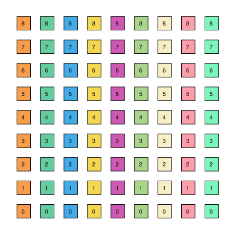
Figure 18: Example of GPU kernel organized by blocks

Let’s say we want to launch a kernel having 16 blocks with 8 threads each. The task that should be performed involves a simple power calculation. Assume that we would like to raise the numbers from 0 to 7 (the thread IDs) to the powers 0 to 15 (the block IDs). To achive this, we can use the following code (see Listing 15).

Listing 15: Example of a function organized by blocks

⬇

1#include <stdio.h>

2

3__device__ int powr(int x, int n) {

4 int res = x;

5 for (int i=n; i>1; --i)

6 res *= x;

7 return (n==0)?1:res;

8}

9

10__global__ void L(){

11 if (threadIdx.x != 0 || blockIdx.x != 0)

12 printf("%d powered to %d is: %d \n", threadIdx.x, blockIdx.x, powr(threadIdx.x, blockIdx.x));

13}

14

15int main() {

16 L<<<8,16>>>();

17 cudaDeviceSynchronize();

18 return 0;

19}

Lines 3-8 define a helper function powr (x,n), which raises $x$ to the power of $n$, where $x$ and $n$ are integers. The kernel function is specified at the lines 10-13. The actual calling of the kernel is made at line 16. As you can see we launch the kernel with parameters 8,16, i.e. 8 blocks with 16 threads each.

Now, we can divide or parallelize a given problem to blocks and threads. However, if you recall the mas problem (Section 3), we have used the prng of the host only. This leaded to a noticeable overhead and over-complication of the problem: we first generated two pseudo-random letters $\psi_{i}$ and $\psi_{j}$, then we pass them to the device as kernel parameters, to further interchange them with all the possible unordered pairs of letters in the corresponding alphabet.

4.2 CUDA as pseudo-random number generator

What if we want to use a prng inside the device? Furthermore, how to be sure that the pseudo-randomly generated numbers inside the threads are not equal? For this a fast and reliable prng is needed. Using the host prng routines is not a wise approach – we have to repeatedly transfer the generated values back and forth from the host to the device.

With the help of the following CUDA code example given in Listing 16, we are going to learn some new techniques:

• How to define and launch multiple kernels inside a single CUDA program.

• How to use the external libraries provided by CUDA.

• How to generate random float numbers by using the device itself.

Listing 16: Parallel CUDA pseudo-random float number generator

⬇

1#include <stdio.h>

2#include <cuda.h>

3#include <curand_kernel.h>

4

5#define B 8

6#define T 8

7

8__global__ void setupKernel(curandState* state, unsigned long seed) {

9 int idx = blockIdx.x*blockDim.x + threadIdx.x;

10 curand_init(seed, idx, 0, &state[idx]);

11}

12

13__global__ void generate(curandState* globalState, float* devRandomValues) {

14 int idx = blockIdx.x*blockDim.x + threadIdx.x;

15 curandState localState = globalState[idx];

16 float randF = curand_uniform(&localState);

17 devRandomValues[idx] = randF;

18 globalState[idx] = localState;

19}

20

21int main() {

22 curandState* devStates;

23 float* randomValues = new float[B*T];

24 float* devRandomValues;

25

26 // we allocate the required memory blocks

27 cudaMalloc(&devStates, B*T*sizeof(curandState));

28 cudaMalloc(&devRandomValues, B*T*sizeof(*randomValues));

29

30 // initial setup

31 setupKernel<<<B,T>>>(devStates, time(NULL));

32 cudaDeviceSynchronize();

33

34 // generator

35 generate<<<B,T>>>(devStates, devRandomValues);

36 cudaDeviceSynchronize();

37

38 // extract the random values from the device

39 cudaMemcpy(randomValues, devRandomValues, B*T*sizeof(*randomValues), cudaMemcpyDeviceToHost);

40

41 // feedback

42 for (int i=0;i<B*T;++i)

43 printf("%f\n", randomValues[i]);

44

45 // cleaning up

46 cudaFree(devRandomValues);

47 cudaFree(devStates);

48 delete randomValues;

49

50 return 0;

51}

First (lines 2-3), we include the CUDA library, as well as the CUDA random kernel headers. For more flexibility, we define the block and thread numbers (lines 5-6) as constants B and T.

The first kernel, which can be found at lines 8-11, is initializing each thread (from the pool of threads) with a unique initial seed. To achieve this we are using the built-in CUDA function curand_init. We save each such seed to the corresponding cell inside the array state.

The second kernel, which is defined at lines 13-19, uses the seed values initialized by the first kernel and the CUDA built-in function curand_uniform to generate a random float number in the interval $\left[0.0,1.0\right]$. We save this value in a corresponding cell inside an array named devRandomValues. Furthermore, we update the seed corresponding to this thread, so each consequent prng yields a different result.

The main function follows the logic introduced during the examples in the previous sections. At lines 27-28 we allocate the device memory blocks:

• a pointer to a device memory block devStates, which is going to save our current thread seeds;

• a device memory block devRandomValues, which is going to save the generated pseudo-random values;

Then, we launch the first kernel (line 31) to initialize the seeds, which is followed by the launch of the second kernel (line 35) to populate the pseudo-randomly generated numbers inside the memory block devRandomValues. The remaining lines were already discussed in the previous examples.

Now, we need to address the following questions:

• How to generate pseudo-random integer numbers in a predefined interval?

• How to utilize the parallel device prngs for automatic cryptanalysis?

4.3 A stand-alone CUDA application to automatically attack MAS ciphertexts

We have all the necessary instruments to construct a complete stand-alone CUDA mas cipher cryptanalysis tool. We will proceed as follows:

1. Setup the CUDA device and initialize a seed for each thread of the GPU.

2. Make a local copy of the encrypted text inside each thread.

3. Initiate a simple hill climbing routine inside each thread by using bigrams. The prngs are launched inside the threads. All prngs are launched independently to guarantee a feed of unique values to the corresponding thread.

4. After passing some predefined threshold value to the hill climbing algorithm, the thread will report back the reached peak value. Then, the results are collected and reported back to the host.

5. The host compares the final scores of all candidates and announces the best one.

Listing 17 contains the complete CUDA source code of the program.

Listing 17: Parallel CUDA monoalphabetic solver with pseudo-random float number generator nested inside the device

⬇

1#include <stdio.h>

2#include <stdlib.h>

3#include <string.h>

4#include <cuda.h>

5#include <curand_kernel.h>

6

7#define encrypted "lwzlmomwmogfeohitkldabztdartw hgylwzlmomwmtrstmmtklfwdtkaslegfxtfmogfaslouflgk egdzofamogflgyassmikttafrywkmitkdgktygkalofustst mmtkgymitgkouofasmtvmmitktdabztlwzlmomwmtralofus tstmmtkfwdtkasgkloufgkmcggkdgktgytaeigkacigstcgk rgkukgwhgyyouwktlegdzofamogfgyegfxtfmogfaslouflg kegdzofamogflgyassmikttgymitlttstdtfml"

8#define encryptedLen ((int)sizeof(encrypted)-1)

9

10#define B 16

11#define T 16

12#define CLIMBINGS 5000

13#define ALPHABET 26

14#define totalBigrams ((int)ALPHABET*ALPHABET)

15

16// a host function to extract and map all the bigrams from a given file

17__host__ void extractBigrams(unsigned long long int *scores) {

18 FILE* bigramsFile = fopen("bigramParsed", "r");

19 while(1){

20 char tempBigram[2];

21 unsigned long long int tempBigramScore = 0;

22 if (fscanf(bigramsFile, "%s %llu", tempBigram, &tempBigramScore) < 2)

23 { break; }

24 scores[(tempBigram[0]-’a’)*ALPHABET + tempBigram[1]-’a’] = tempBigramScore;

25 }

26 fclose(bigramsFile);

27}

28

29// demap and print a given array of integer letters

30__host__ __device__ void demap(int* encrMap, int length) {

31 for (int j=0; j<length; ++j) {

32 printf("%c", encrMap[j] + ’a’);

33 }

34 printf("\n");

35}

36

37// calculate a bigram score of a given decrypted (mapped) candidate

38__host__ unsigned long long int candidateScore(int* decrMsg, int length, unsigned long long int* scores) {

39 unsigned long long int total = 0;

40 for (int j=0; j<length-1; ++j) {

41 total += scores[ALPHABET*decrMsg[j] + decrMsg[j+1]];

42 }

43 return total;

44}

45

46__global__ void setupKernel(curandState* state, unsigned long seed) {

47 int idx = blockIdx.x*blockDim.x + threadIdx.x;

48 curand_init(seed, idx, 0, &state[idx]);

49}

50

51__global__ void K(unsigned long long int *d_scores, int *d_encrypted, curandState* globalState, int *d_decrypted){

52 int* localBufferEncrypted = new int[encryptedLen];

53 for (int j=0; j<encryptedLen; ++j)

54 localBufferEncrypted[j] = d_encrypted[j];

55 int idx = blockIdx.x*blockDim.x + threadIdx.x;

56 curandState localState = globalState[idx];

57

58 long long int delta = 0;

59 float randF = 0;

60 int leftLetter = 0;

61 int rightLetter = 0;

62 int pair[2];

63

64 for (int cycles=0; cycles<CLIMBINGS; ++cycles) {

65 delta = 0;

66 randF = curand_uniform(&localState);

67 leftLetter = randF*ALPHABET;

68 rightLetter = leftLetter;

69 while (rightLetter == leftLetter) {

70 randF = curand_uniform(&localState);

71 rightLetter = randF*ALPHABET;

72 }

73

74 for (int j=0; j<encryptedLen-1; ++j)

75 {

76 pair[0] = localBufferEncrypted[j];

77 pair[1] = localBufferEncrypted[j+1];

78 delta -= d_scores[ALPHABET*pair[0] + pair[1]];

79

80 if (pair[0] == leftLetter)

81 pair[0] = rightLetter;

82 else if (pair[0] == rightLetter)

83 pair[0] = leftLetter;

84

85 if (pair[1] == leftLetter)

86 pair[1] = rightLetter;

87 else if (pair[1] == rightLetter)

88 pair[1] = leftLetter;

89 delta += d_scores[ALPHABET*pair[0] + pair[1]];

90 }

91

92 if (delta > 0) {

93 for (int j=0; j<encryptedLen; ++j) {

94 if (localBufferEncrypted[j] == leftLetter)

95 localBufferEncrypted[j] = rightLetter;

96 else if (localBufferEncrypted[j] == rightLetter)

97 localBufferEncrypted[j] = leftLetter;

98 }

99 }

100 }

101

102 for (int j=0; j<encryptedLen; ++j)

103 d_decrypted[idx*encryptedLen+j] = localBufferEncrypted[j];

104 delete localBufferEncrypted;

105}

106

107int main() {

108

109 int threads = B*T;

110 int encryptedMap[encryptedLen];

111

112 // we map the encrypted message to integers

113 for (int j=0; j<encryptedLen; ++j)

114 encryptedMap[j] = encrypted[j] - ’a’;

115

116 unsigned long long int scores[totalBigrams];

117 extractBigrams(scores);

118

119 unsigned long long int *d_scores;

120 int *d_encrypted, *d_decrypted;

121 int* decrypted = new int[encryptedLen*threads];

122

123 // allocate memory blocks on the device

124 cudaMalloc((void **)&d_scores, sizeof(unsigned long long int)*totalBigrams);

125 cudaMalloc((void **)&d_encrypted, sizeof(int)*encryptedLen);

126 cudaMalloc((void **)&d_decrypted, sizeof(int)*encryptedLen*threads);

127

128 // copy the scores array and encrypted msg array to the device memory

129 cudaMemcpy(d_scores, scores, sizeof(unsigned long long int)*totalBigrams, cudaMemcpyHostToDevice);

130 cudaMemcpy(d_encrypted, encryptedMap, sizeof(int)*encryptedLen, cudaMemcpyHostToDevice);

131

132 // we allocate the required memory blocks for pseudo-random generation routines

133 curandState* devStates;

134 cudaMalloc(&devStates, B*T*sizeof(curandState));

135

136 // initial setup

137 setupKernel<<<B,T>>>(devStates, time(NULL));

138 cudaDeviceSynchronize();

139

140

141 // the "flock" of threads initiating automatic cryptanalysis in parallel

142 K<<<B,T>>>(d_scores, d_encrypted, devStates, d_decrypted);

143 cudaDeviceSynchronize();

144

145 // copy the results array back to the host memory

146 cudaMemcpy(decrypted, d_decrypted, sizeof(int)*encryptedLen*threads, cudaMemcpyDeviceToHost);

147

148 int bestCandidate = 0;

149 unsigned long long int bestScore = 0;

150

151 // we extract the best candidate among all threads

152 for (int j=0; j<threads; ++j) {

153 unsigned long long int currentScore = candidateScore(&decrypted[encryptedLen*j], encryptedLen, scores);

154 if (currentScore > bestScore) {

155 bestScore = currentScore;

156 bestCandidate = j;

157 }

158 }

159

160 // final solution output

161 printf("Best candidate score: %llu\n", bestScore);

162 demap(&decrypted[encryptedLen*bestCandidate], encryptedLen);

163

164 // we free the allocated device and host memory blocks

165 cudaFree(d_scores);

166 cudaFree(d_encrypted);

167 cudaFree(d_decrypted);

168 cudaFree(devStates);

169 delete decrypted;

170

171 return 0;

172

173}

Now, let’s trace the program behavior by employing the useful memory snapshot approach. At lines 7-14 we define several constants we are going to use throughout the program logic. A summary of all the constants is given in Table 1.

Table 1: Overview of the predefined constants

Constant	Logic
encrypted	the encrypted text
encryptedLen	the length of the encrypted text
B	the number of blocks
T	the number of threads
CLIMBINGS	the threshold value of hill climbing tries for each distinct thread
ALPHABET	the total count of letters in the current alphabet
totalBigrams	the total count of distinct bigrams

The current snapshot of the host and device memory blocks, up to line 123, is given in Figure 19.

Figure 19: Initial pointers and diagram.

As usual, we setup the necessary pointers. For simplicity, we denote the variable type unsigned long long int with ulli. Furthermore, we denote the variable encryptedLen as LL.

The functions extractBigrams() (lines 17-27) and demap() (lines 29-35) are the same as those inside the previous implementation of the mas cryptanalysis tool (see Listing 14). However, we introduce a new function named candidateScore (lines 38-49), which is going to return the bigram score of a given string.

After that, as defined at lines 124-131 we first allocate and then transfer the data needed to be accessible through the GPU kernel routines (see Figure 20).

Figure 20: Allocations and transfers.

We first allocate an ulli array, which is going to keep the scores inside the device memory as well. Then, we proceed with allocating two additional int arrays: the first will keep the encrypted text (the second row-block from the device memory block), while the second will keep all the decrypted candidates yielded by all the B*T threads (the third row-block in the device memory). Then, depicted by gray dotted arrows, we transfer the bigrams score from the host to the device , as well as the encrypted message itself.

We are ready to setup the device built-in prng (lines 133-138). The current memory block snapshot of the host and the device is given in Figure 21.

Figure 21: Launching the first kernel.

We allocate a curandState array, having size B*T equal to the number of device threads, which is going to hold down the initial seeds of the device built-in prng. Then, we launch the kernel setupKernel which populates the curandState device array with the provided by the kernel seeds. When a given thread with global index $I$ needs a pseudo-randomly generated number, it directly communicates with cell indexed $I$ inside the curandState device array. Moreover, after each call, the cell with index $I$ is updated to guarantee an infinite stream of pseudo-randomly generated numbers.

We are ready to launch the hill climbing routine device kernel K (line 142). Next, we transfer back (from the device to the host memory) the local optimums yielded by each device thread. The snapshot is given in Figure 22.

Figure 22: Launching the second kernel.

Once the kernel setupKernel finished, we launch the kernel K. Each device thread is working with its own copy of the encrypted text and therefore each thread yields its own local optimum of the decrypted candidate. During the hill climbing routine, each thread is independently generating and utilizing pseudo-random numbers by querying its corresponding curandState cell. Once the thread finished, the respective local optimum is written down in the device memory block (the third row). Finally, all the local optimums are transferred back to the host, by using the dedicated integer array decrypted.

Once the host integer array decrypted has been populated with the local optimums yielded by the device threads, we pick the best one and announce it as a solution. However, before doing that, we should make sure that all the threads had finished their hill climbing routines by synchronizing the threads (see line 143 from Listing 17). We are ready to un-allocate the used memory blocks (see Figure 23).

Figure 23: Un-allocation.

We consequently un-allocate all the device memory blocks we have used throughout the automatic cryptanalysis routines (see lines 165-168 from Listing 17). However, as shown in line 169, we further need to free the dynamically allocated memory blocks from the host as well. Since the array decrypted was created dynamically (line 121) we further clean it by calling the host delete operator.

Now, let’s go back and inspect the new version of the kernel K. We start with copying the original encrypted message to the GPU thread (lines 52-54 from Listing 17). Then, we extract the unique thread identification number (line 55), initialize and load the seed from the device global memory (line 56), initialize some helper variables (lines 58-62) and initiate the hill climbing routines (lines 64-100).

Each climbing try starts with resetting the delta variable to 0. Then, we generate a random float number by using the thread seed (line 66) and further convert it to an integer number in the interval [0,26)(line 67). We repeat the process to get another distinct integer number in the same interval (lines 68-72). Those numbers are saved in two variables named leftLetter and rightLetter.

At lines 74-88 we interchange all occurrences of the letter leftLetter inside the encrypted text with the letter rightLetter and vice versa. The variable delta is tracing the score change when the old bigram (line 78) is interchanged with the new one (line 89). Indeed, if the overall sum of deltas is greater than zero, then the newly created candidate is better than the old one and we update it accordingly (that’s why we have created a local copy of the encrypted text in the first place). This is visible at lines 92-100. We further save the best thread candidate to the device global memory, so we can later extract it by the host.

Most of the routines inside the main function were already discussed in the previous sections. At the end of the function, at lines 148-158, we further extract the best candidate among all thread final candidates and print it to the terminal (line 162).

The parallel hill climbing approach can be illustrated by the visualization shown in Figure 24. Each circle represents a local maximum, i.e. a peak, while the color of the circle corresponds to the peak altitude – lower values are colored in cold colors (nuances of blue), while the higher values are represented with hot colors (nuances of red).

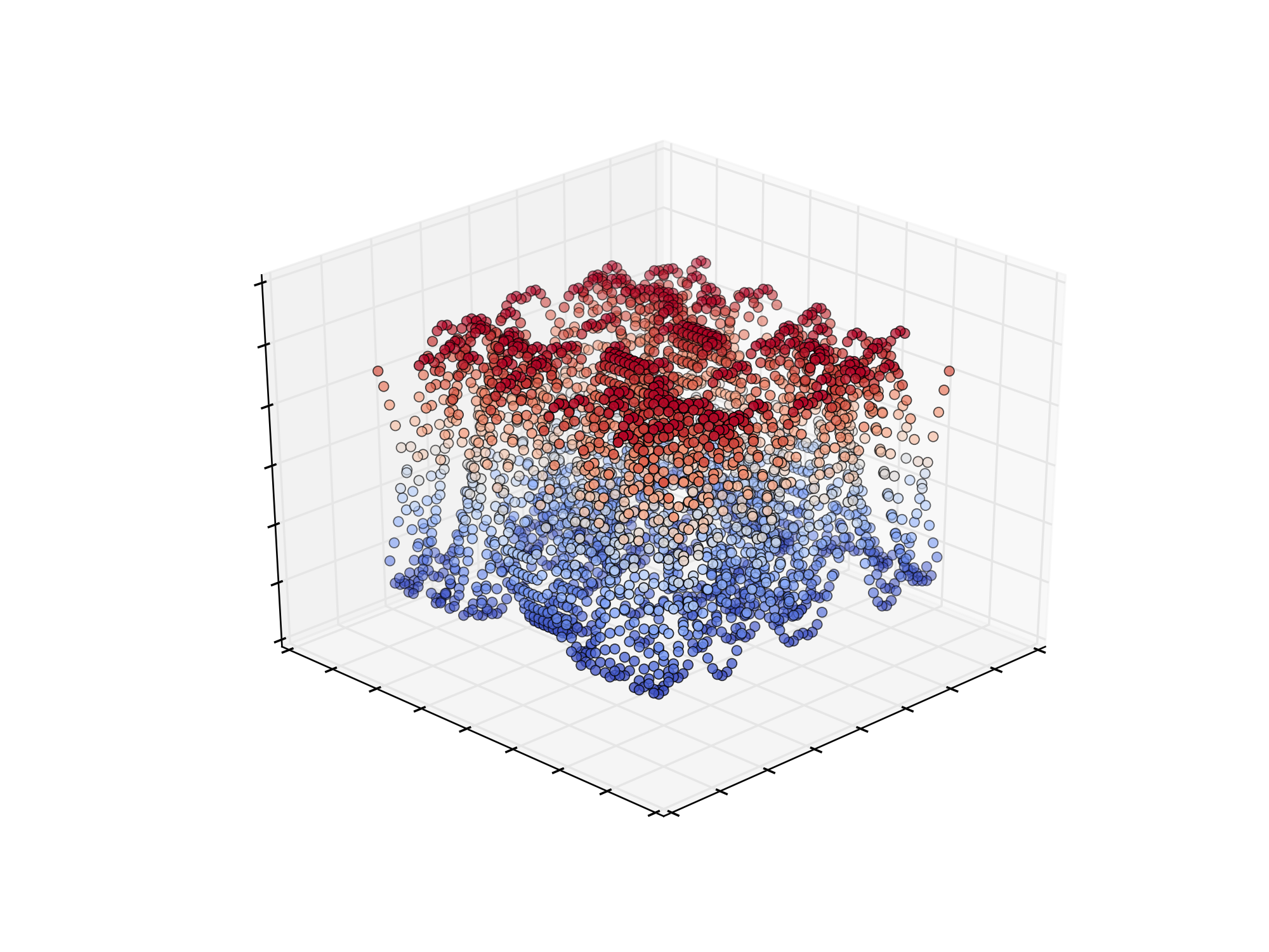
Figure 24: Example of CUDA parallel hill-climbing discretization

Each thread of the CUDA device is to be attracted by some of those peaks. Then, the peaks are further collected to make measurements of their exact altitude in order to announce the best candidate.

Now, let’s compile and run the source code given in Listing 17. Can you decrypt the provded encrypted text? Who is the original author of the plain text?

Finally, you could try to decrypt the message given in Listing 14 as well. What was the success ratio, i.e. the number of times you execute the program versus the number of times the global solution has been found?

5 CUDA memory model and CUDA error handling

This section briefly discusses a simple way to catch CUDA related errors after a given kernel launch. Besides that, we will take a look into the hierarchy of the CUDA memory model to emphasize its importance.

There are several types of memory blocks inside a given CUDA device. Table 2 gives an overview of these types. A more detailed introduction to the CUDA memory hierarchy could be found in [NVIDIA, 2021a].

Table 2: Overview of the types of memory blocks in a CUDA device

Memory	Encapsulation	Size	Latency
Local	Per Thread	Limited	Small
Shared	Per Block	Mediocre	Medium
Global	Per Device	Huge	High

The variables defined inside the kernel are normally saved inside the local memory (composed of registers). Let’s assume that we have a total of $T$ threads to be launched by some CUDA kernel. Furthermore, each thread requires a total of $X$ bytes to be allocated. So, we have a total of $T*X$ bytes that need to be situated inside the CUDA core registers. If we have a total of $C$ CUDA cores, each having a fixed number of available size of registers of $Y$ bytes, the total available CUDA core register size is $C*Y$. What happen if $T*X>C*Y$? This possible scenario is defined as registers spilling and the extra required memory is allocated on the global memory. However, this greatly reduce the software performance.

During our construction of the CUDA cryptanalysis tools we ignored the memory model. We left that optimization to the CUDA compiler. Now, let’s update the CUDA kernel of our previous example to benefit from the shared memory (see Listing 18).

Listing 18: Parallel CUDA pseudo-random float number generator kernel, optimized by shared memory utilization

⬇

1__global__ void K(unsigned long long int *d_scores, int *d_encrypted, int encryptedLen, curandState* globalState, int *d_decrypted){

2

3 __shared__ unsigned long long int shared_scores[ALPHABET*ALPHABET];

4

5 int* localBufferEncrypted = new int[encryptedLen];

6 for (int j=0; j<encryptedLen; ++j)

7 localBufferEncrypted[j] = d_encrypted[j];

8 int idx = blockIdx.x*blockDim.x + threadIdx.x;

9

10 if (threadIdx.x <= 25) {

11 for (int j=0; j<ALPHABET; ++j)

12 shared_scores[threadIdx.x*ALPHABET + j] = d_scores[threadIdx.x*ALPHABET + j];

13 }

14

15 __syncthreads();

16

17 curandState localState = globalState[idx];

18

19 long long int delta = 0;

20 float randF = 0;

21 int leftLetter = 0;

22 int rightLetter = 0;

23 int pair[2];

24

25 for (int cycles=0; cycles<CLIMBINGS; ++cycles) {

26 delta = 0;

27 randF = curand_uniform(&localState);

28 leftLetter = randF*ALPHABET;

29 rightLetter = leftLetter;

30 while (rightLetter == leftLetter) {

31 randF = curand_uniform(&localState);

32 rightLetter = randF*ALPHABET;

33 }

34

35 for (int j=0; j<encryptedLen-1; ++j)

36 {

37 pair[0] = localBufferEncrypted[j];

38 pair[1] = localBufferEncrypted[j+1];

39 delta -= shared_scores[ALPHABET*pair[0] + pair[1]];

40

41 if (pair[0] == leftLetter)

42 pair[0] = rightLetter;

43 else if (pair[0] == rightLetter)

44 pair[0] = leftLetter;

45

46 if (pair[1] == leftLetter)

47 pair[1] = rightLetter;

48 else if (pair[1] == rightLetter)

49 pair[1] = leftLetter;

50

51 delta += shared_scores[ALPHABET*pair[0] + pair[1]];

52 }

53

54 if (delta > 0) {

55 for (int j=0; j<encryptedLen; ++j) {

56 if (localBufferEncrypted[j] == leftLetter)

57 localBufferEncrypted[j] = rightLetter;

58 else if (localBufferEncrypted[j] == rightLetter)

59 localBufferEncrypted[j] = leftLetter;

60 }

61 }

62 }

63

64 for (int j=0; j<encryptedLen; ++j)

65 d_decrypted[idx*encryptedLen+j] = localBufferEncrypted[j];

66}

As shown at line 3 we declare an array named shared_scores, which is going to be visible to all the threads inside the given block. At lines 10-13 we partially redistribute the transfer of the bigram scores from the global memory (d_scores array) to the shared memory. Having this in mind, we need to synchronize all the threads before stepping into the next source code fragments (line 15). If we fail to do that, there is a great chance for some subset of threads to start reading parts of the shared memory block with undefined values. Then, we proceed with the bigram scoring routines as usual, but this time extracting the scores from the shared memory instead of the global one (lines 39 and 51).

This simple utilization of the device shared memory resulted in considerable speed improvements. For example, during our experiments, an encrypted text with length 471 symbols is decrypted on average in 1.1 seconds by using a mid-range GPU device and global memory only. However, by exploiting the shared memory utilization we did that in less than 0.5 seconds.

In order to squeeze out the best of a given CUDA capable device we need to tune up the thread and number values. Now, introducing the shared memory concept it makes sense to organize the threads into blocks. However, we should pay attention to the technical parameters of the CUDA device. Otherwise, we can end up in the situation with unpredictable semantic errors. Nevertheless, we can catch some of those errors by using the following error handle fragment after each CUDA kernel launch (see Listing 19):

Listing 19: Example of error handling in CUDA, optimized by shared memory utilization

⬇

1cudaError_t error = cudaGetLastError();

2 if (error != cudaSuccess) {

3 printf("CUDA error: %s\n", cudaGetErrorString(error));

4 exit(-1);

5 }

6 Dynamical vs static GPU memory allocation

The automatic cryptanalysis tool presented in Listing 17 was constructed in a flexible way, which, for example, allows us to re-configure the source code to be applicable for another encrypted text with different length by minimum efforts. However, to achieve this we used a technique which is more common for CPU programming, not GPU, i.e. dynamic memory allocation.

We can significantly improve the performance of the GPU device if dynamic memory allocation routines are avoided. Listing 20 contains the complete CUDA source code of the static implementation of the solver.

This time the need of dynamically memory allocation is avoided by exploiting the C/CUDA preprocessor directives (see lines 7-15). Compile and run the source code in Listing 20. Can you recover the plaintext of the encrypted message?

Listing 20: Final CUDA implementation for automatic cryptanalysis of text encrypted by mas, optimized by shared memory utilization

⬇

1#include <stdio.h>

2#include <stdlib.h>

3#include <string.h>

4#include <cuda.h>

5#include <curand_kernel.h>

6

7#define B ((int)16)

8#define T ((int)26)

9#define THREADS ((int)B*T)

10#define CLIMBINGS ((int)5000)

11#define ALPHABET ((int)26)

12#define totalBigrams ((int)ALPHABET*ALPHABET)

13

14#define encrypted "djrggrygdudrdunkluejqxgahbvhxbixnadjng qniqwdxqaqguaeouludbdndjngqsjngqlnaeoulhdunktqiuqghkbnxtu khxbaqdjntnihkhobgughktsjngqgnordunkxqmruxqgdjqenggqggunk nionkzaqgghzqghktarljduaqhktgdrtbinxdrkhdqobdjqanxqtuiiul rodgrygdudrdunkluejqxghxqxhxqobrgqtinxauoudhxberxengqgnkh llnrkdnidjqduaqhktlhxqxqmruxqtinxqkluejqxukzhkttqluejqxukz"

15#define ENCRYPTEDLEN ((int)sizeof(encrypted)-1)

16

17__host__ void extractBigrams(long long int *scores) {

18 FILE* bigramsFile = fopen("bigramParsed", "r");

19 while(1){

20 char tempBigram[2];

21 long long int tempBigramScore = 0;

22 if (fscanf(bigramsFile, "%s %llu", tempBigram, &tempBigramScore) < 2)

23 { break; }

24 scores[(tempBigram[0]-’a’)*ALPHABET + tempBigram[1]-’a’] = tempBigramScore;

25 }

26 fclose(bigramsFile);

27}

28

29__host__ int getMaxElement(long long int *scores, int length) {

30 long long int tempMaxScore = 0;

31 int tempIndex = 0;

32 for (int j=0; j<length; ++j) {

33 if (scores[j] > tempMaxScore) {

34 tempIndex = j;

35 tempMaxScore = scores[j];

36 }

37 }

38 return tempIndex;

39}

40

41__host__ __device__ void demap(int* encrMap) {

42 for (int j=0; j<ENCRYPTEDLEN; ++j) {

43 printf("%c", encrMap[j] + ’a’);

44 }

45 printf("\n");

46}

47

48__host__ long long int candidateScore(int* decrMsg, long long int* scores) {

49 long long int total = 0;

50 for (int j=0; j<ENCRYPTEDLEN-1; ++j) {

51 total += scores[ALPHABET*decrMsg[j] + decrMsg[j+1]];

52 }

53 return total;

54}

55

56__global__ void setupKernel(curandState* state, long seed) {

57 int idx = blockIdx.x*blockDim.x + threadIdx.x;

58 curand_init(seed, idx, 0, &state[idx]);

59}

60

61__global__ void K(long long int *d_scores, int *d_encrypted, curandState* globalState, int *d_decrypted){

62

63 __shared__ long long int shared_scores[totalBigrams];

64

65 int localBufferEncrypted[ENCRYPTEDLEN];

66 for (int j=0; j<ENCRYPTEDLEN; ++j)

67 localBufferEncrypted[j] = d_encrypted[j];

68 int idx = blockIdx.x*blockDim.x + threadIdx.x;

69

70 if (threadIdx.x <= 25) {

71 for (int j=0; j<ALPHABET; ++j)

72 shared_scores[threadIdx.x*ALPHABET + j] = d_scores[threadIdx.x*ALPHABET + j];

73 }

74

75 __syncthreads();

76

77 curandState localState = globalState[idx];

78

79 long long int delta = 0;

80 float randF = 0;

81 int leftLetter = 0;

82 int rightLetter = 0;

83 int pair[2];

84

85 for (int cycles=0; cycles<CLIMBINGS; ++cycles) {

86 delta = 0;

87 randF = curand_uniform(&localState);

88 leftLetter = randF*ALPHABET;

89 rightLetter = leftLetter;

90 while (rightLetter == leftLetter) {

91 randF = curand_uniform(&localState);

92 rightLetter = randF*ALPHABET;

93 }

94

95 for (int j=0; j<ENCRYPTEDLEN-1; ++j)

96 {

97 pair[0] = localBufferEncrypted[j];

98 pair[1] = localBufferEncrypted[j+1];

99 delta -= shared_scores[ALPHABET*pair[0] + pair[1]];

100

101 if (pair[0] == leftLetter)

102 pair[0] = rightLetter;

103 else if (pair[0] == rightLetter)

104 pair[0] = leftLetter;

105

106 if (pair[1] == leftLetter)

107 pair[1] = rightLetter;

108 else if (pair[1] == rightLetter)

109 pair[1] = leftLetter;

110

111 delta += shared_scores[ALPHABET*pair[0] + pair[1]];

112 }

113

114 if (delta > 0) {

115 for (int j=0; j<ENCRYPTEDLEN; ++j) {

116 if (localBufferEncrypted[j] == leftLetter)

117 localBufferEncrypted[j] = rightLetter;

118 else if (localBufferEncrypted[j] == rightLetter)

119 localBufferEncrypted[j] = leftLetter;

120 }

121 }

122 }

123

124 for (int j=0; j<ENCRYPTEDLEN; ++j)

125 d_decrypted[idx*ENCRYPTEDLEN+j] = localBufferEncrypted[j];

126

127}

128

129int main() {

130

131 int encryptedMap[ENCRYPTEDLEN];

132

133 for (int j=0; j<ENCRYPTEDLEN; ++j)

134 encryptedMap[j] = encrypted[j] - ’a’;

135

136 long long int scores[totalBigrams];

137 extractBigrams(scores);

138

139 long long int *d_scores;

140 int *d_encrypted, *d_decrypted;

141 static int decrypted[ENCRYPTEDLEN*THREADS];

142

143 cudaMalloc((void **)&d_scores, sizeof(long long int)*totalBigrams);

144 cudaMalloc((void **)&d_encrypted, sizeof(int)*ENCRYPTEDLEN);

145 cudaMalloc((void **)&d_decrypted, sizeof(int)*ENCRYPTEDLEN*THREADS);

146

147 cudaError_t error = cudaGetLastError();

148 if (error != cudaSuccess) {

149 printf("CUDA error (1): %s\n", cudaGetErrorString(error));

150 exit(-1);

151 }

152

153 cudaMemcpy(d_scores, scores, sizeof(long long int)*totalBigrams, cudaMemcpyHostToDevice);

154 cudaMemcpy(d_encrypted, encryptedMap, sizeof(int)*ENCRYPTEDLEN, cudaMemcpyHostToDevice);

155

156 error = cudaGetLastError();

157 if (error != cudaSuccess) {

158 printf("CUDA error (2): %s\n", cudaGetErrorString(error));

159 exit(-1);

160 }

161

162 curandState* devStates;

163 cudaMalloc(&devStates, THREADS*sizeof(curandState));

164

165 error = cudaGetLastError();

166 if (error != cudaSuccess) {

167 printf("CUDA error (3): %s\n", cudaGetErrorString(error));

168 exit(-1);

169 }

170

171 setupKernel<<<B,T>>>(devStates, time(NULL));

172 cudaDeviceSynchronize();

173

174 error = cudaGetLastError();

175 if (error != cudaSuccess) {

176 printf("CUDA error (4): %s\n", cudaGetErrorString(error));

177 exit(-1);

178 }

179

180 K<<<B,T>>>(d_scores, d_encrypted, devStates, d_decrypted);

181 cudaDeviceSynchronize();

182

183 error = cudaGetLastError();

184 if (error != cudaSuccess) {

185 printf("CUDA error (5): %s\n", cudaGetErrorString(error));

186 exit(-1);

187 }

188

189 cudaMemcpy(decrypted, d_decrypted, sizeof(int)*ENCRYPTEDLEN*THREADS, cudaMemcpyDeviceToHost);

190

191 int bestCandidate = 0;

192 long long int bestScore = 0;

193

194 for (int j=0; j<THREADS; ++j) {

195 long long int currentScore = candidateScore(&decrypted[ENCRYPTEDLEN*j], scores);

196 if (currentScore > bestScore) {

197 bestScore = currentScore;

198 bestCandidate = j;

199 }

200 }

201

202 printf("Best candidate score: %llu\n", bestScore);

203 demap(&decrypted[ENCRYPTEDLEN*bestCandidate]);

204

205 cudaFree(d_scores);

206 cudaFree(d_encrypted);

207 cudaFree(d_decrypted);

208 cudaFree(devStates);

209

210 return 0;

211}

7 Used principles and comparison to other implementations

This Section summarizes the improvements made throughout the tutorial. Then, by following the design principles outlined during the previous sections, a stand-alone CUDA application for automatic cryptanalysis of ciphertexts encrypted by sct is presented. At the end the provided GPU routine is compared with CT2 [Esslinger, 2009]: a state-of-the-art cryptanalysis tool.

7.1 Generalization of principles

Throughout this tutorial, we addressed common issues, which arose from translating a given problem from the domain of classical cryptanalysis to the domain of general-purpose computations on graphics processing units (GPGPU). Step by step, by introducing technical optimization and mathematical insights, we built an efficient stand-alone framework. Let’s summarize the most critical improvements we made:

• Reducing the overhead caused by the host-device communication (Section 3.1): The first optimization issue was caused by the bandwidth overhead, generated from the communication between the host and the device. This, for example, is illustrated in Listing 7. We pick two different random letters, pass them to the GPU kernel, which logically divides the work to the 325 threads. Then, the best score is fetched and we repeat this process 500 times. However, this creates additional bandwidth overhead as we repeatedly send packets back and forth between the device and the host. To get rid of this undesired behavior, we made the following changes:

  • The prng was reallocated from the CPU to the GPU itself (Section 4.2).

  • The CUDA application was switched to an heuristic version and the host-device bandwidth was optimized. Due to this modification, the hill climbing routine is launched only once (Section 4.3).

• Utilizing a metaheuristic approach, which is both: highly effective in solving the problem and is efficiently implemented to split the overall work between different GPU cores. Various nuances of metaheuristics were exploited throughout the tutorial. We first started with best neighbor hill climbing approach (Section 3.3). Then, we migrated to the better neighbor metaheuristic (Section 4.3). This migration was possible by encapsulating the prng to the GPU device.

• Synchronizing the threads (Section 4.3): Synchronization was achieved by using the following techniques:

  • Each thread starts from a pseudo-random state. Hence, the key space is randomly crawled.

  • Each thread is a stand-alone, i.e. it is capable of performing the full instance of the algorithm entirely by itself.

• Using faster memory when possible (Section 5): The most-frequently used memory read operations were migrated to the device shared memory space.

• Avoiding dynamic memory allocations (Section 6).

7.2 A stand-alone CUDA application for automatic ciphertext-only attacks against sct

Following these design principles, the last example (see Listing 20) was slightly modified to be launched on a more complex problem, the cryptanalysis of the Single-columnar transposition sct cipher. An introduction, as well as an overview of the state-of-the-art attacks on the sct cipher, can be found in the PhD thesis of G. Lasry [Lasry, 2018]. The source code in Listing 21 is a CUDA implementation for automatic cryptanalysis of encrypted by sct.

Listing 21: Automatic cryptanalysis of ciphertext encrypted by sct

⬇

1#include <stdio.h>

2#include <stdlib.h>

3#include <string.h>

4#include <cuda.h>

5#include <curand_kernel.h>

6

7#define B ((int)32)

8#define T ((int)32)

9#define THREADS ((int)B*T)

10#define CLIMBINGS 150000

11#define ALPHABET 26

12#define totalBigrams ((int)ALPHABET*ALPHABET)

13#define CAP ((float)999999.0)

14

15#define ENCRYPTED_T "tteohtedanisroudesereguwocubsoit oabbofeiaiutsdheeisatsarsturesuaastniersrotnesctrctxd iwmhcusyenorndasmhaipnnptmaeecspegdeislwoheoiymreeotb sspiatoanihrelhwctftrhpuunhoianunreetrioettatlsnehtba ecpvgtltcirottonesnobeeeireaymrtohaawnwtesssvassirsrh abapnsynntitsittchitoosbtelmlaouitrehhwfeiaandeitcieg freoridhdcsheucrnoihdeoswobaceeaorgndlstigeearsotoetd uedininttpedststntefoeaheoesuetvmmiorftuuhsurof"

16#define ENCRYPTEDLEN ((int)sizeof(ENCRYPTED_T)-1)

17

18#define KEY_LENGTH 30

19#define SECTION_CONSTANT ENCRYPTEDLEN/KEY_LENGTH

20

21#define HEUR_THRESHOLD_OP1 50

22#define HEUR_THRESHOLD_OP2 70

23

24#define OP1_HOP 4

25#define OP2_HOP 2

26

27__host__ void extractBigrams(float *scores) {

28 FILE* bigramsFile = fopen("log2", "r");

29 while(1){

30 char tempBigram[2];

31 float tempBigramScore = 0.0;

32 if (fscanf(bigramsFile, "%s %f", tempBigram, &tempBigramScore) < 2)

33 { break; }

34 scores[(tempBigram[0]-’a’)*ALPHABET + tempBigram[1]-’a’] = tempBigramScore;

35 }

36 fclose(bigramsFile);

37}

38

39__host__ __device__ void demap(int* encrMap) {

40 for (int j=0; j<ENCRYPTEDLEN; ++j) {

41 printf("%c", encrMap[j] + ’a’);

42 }

43 printf("\n");

44}

45

46__host__ float candidateScore(int* decrMsg, float* scores) {

47 float total = 0.0;

48 for (int j=0; j<ENCRYPTEDLEN-1; ++j)

49 total += scores[ALPHABET*decrMsg[j] + decrMsg[j+1]];

50 return total;

51}

52

53__global__ void setupKernel(curandState* state, unsigned long seed) {

54 int idx = blockIdx.x*blockDim.x + threadIdx.x;

55 curand_init(seed, idx, 0, &state[idx]);

56}

57

58__device__ __host__ void decrypt(int* encrypted, int* key, int* decrypted) {

59

60 int columns[KEY_LENGTH][SECTION_CONSTANT+1];

61 int offset = 0;

62 int colLength[KEY_LENGTH];

63

64 for (int j=0; j<KEY_LENGTH; ++j) {

65 colLength[j] = ENCRYPTEDLEN / KEY_LENGTH;

66 if (j < ENCRYPTEDLEN % KEY_LENGTH)

67 colLength[j]++;

68 }

69

70 for (int keyPos=0; keyPos < KEY_LENGTH; ++keyPos) {

71 offset = 0;

72 for (int i=0; i<KEY_LENGTH; ++i)

73 if (key[i] < key[keyPos])

74 offset += colLength[i];

75

76 for (int j=0; j<colLength[keyPos]; ++j)

77 columns[key[keyPos]][j] = encrypted[offset+j];

78 }

79

80 for (int j=0; j<ENCRYPTEDLEN; ++j)

81 decrypted[j] = columns[key[j % KEY_LENGTH]][j / KEY_LENGTH];

82}

83

84__device__ void swapElements(int *key, int posLeft, int posRight) {

85 if (posLeft != posRight)

86 {

87 key[posLeft] -= key[posRight];

88 key[posRight] += key[posLeft];

89 key[posLeft] = key[posRight] - key[posLeft];

90 }

91}

92

93__device__ void swapBlock(int *key, int posLeft, int posRight, int length) {

94 for (int i=0; i<length; i++)

95 swapElements(key, (posLeft+i)%KEY_LENGTH, (posRight+i)%KEY_LENGTH);

96}

97

98__global__ void K(float *d_scores, int *d_encrypted, curandState* globalState, int *d_decrypted){

99

100 __shared__ float shared_scores[ALPHABET*ALPHABET];

101

102 int key[KEY_LENGTH];

103 int localDecrypted[ENCRYPTEDLEN];

104 int bestLocalDecrypted[ENCRYPTEDLEN];

105 int idx = blockIdx.x*blockDim.x + threadIdx.x;

106 curandState localState = globalState[idx];

107 int leftLetter = 0;

108 int rightLetter = 0;

109 int backupKey[KEY_LENGTH];

110 int shiftHelper[KEY_LENGTH];

111 int blockStart, blockEnd;

112 int l,f,t,t0,n,ff,tt;

113 float tempScore = 0.0;

114 float bestScore = CAP;

115 int j = 0, jj = 0;

116

117 if (threadIdx.x == 0) {

118 for (j=0; j<ALPHABET;++j)

119 for (jj=0; jj<ALPHABET; ++jj)

120 shared_scores[j*ALPHABET + jj] = d_scores[j*ALPHABET + jj];

121 }

122

123 __syncthreads();

124

125 for (j=0; j<KEY_LENGTH; ++j)

126 key[j]=j;

127

128 for (j=0; j<KEY_LENGTH; ++j) {

129 swapElements(key, j, curand_uniform(&localState)*KEY_LENGTH);

130 }

131

132 for (int cycles=0; cycles<CLIMBINGS; ++cycles) {

133

134 for (j=0; j<KEY_LENGTH;j++)

135 backupKey[j] = key[j];

136

137 tempScore = 0.0;

138

139 int branch = curand_uniform(&localState)*100;

140

141 if (branch < HEUR_THRESHOLD_OP1)

142 {

143 for (j=0; j<1+curand_uniform(&localState)*OP1_HOP; j++)

144 {

145 leftLetter = curand_uniform(&localState)*KEY_LENGTH;

146 rightLetter = curand_uniform(&localState)*KEY_LENGTH;

147 swapElements(key, leftLetter, rightLetter);

148 }

149 }

150

151 else if (branch < HEUR_THRESHOLD_OP2)

152 {

153 for (j=0; j< 1+curand_uniform(&localState)*OP2_HOP;j++)

154 {

155 blockStart = curand_uniform(&localState)*KEY_LENGTH;

156 blockEnd = curand_uniform(&localState)*KEY_LENGTH;

157 swapBlock(key, blockStart, blockEnd, 1+curand_uniform(&localState)*(abs((blockStart-blockEnd))-1));

158 }

159 }

160

161 else

162 {

163 l = 1 + curand_uniform(&localState)*(KEY_LENGTH-2);

164 f = curand_uniform(&localState)*(KEY_LENGTH-1);

165 t = (f+1+(curand_uniform(&localState)*(KEY_LENGTH-2)));

166 t = t % KEY_LENGTH;

167

168 for (j=0; j< KEY_LENGTH;j++)

169 shiftHelper[j] = key[j];

170

171 t0 = (t-f+KEY_LENGTH) % KEY_LENGTH;

172 n = (t0+l) % KEY_LENGTH;

173

174 for (j=0; j<n;j++)

175 {

176 ff = (f+j) % KEY_LENGTH;

177 tt = (((t0+j)%n)+f)%KEY_LENGTH;

178 key[tt] = shiftHelper[ff];

179 }

180 }

181

182 decrypt(d_encrypted, key, localDecrypted);

183

184 for (j=0; j<ENCRYPTEDLEN-1; ++j) {

185 tempScore += shared_scores[ALPHABET*localDecrypted[j] + localDecrypted[j+1]];

186 }

187

188 if (tempScore < bestScore) {

189 bestScore = tempScore;

190 for (j=0; j<ENCRYPTEDLEN; ++j) {

191 bestLocalDecrypted[j] = localDecrypted[j];

192 }

193 }

194

195 else

196 {

197 for (j=0; j<KEY_LENGTH;j++)

198 key[j] = backupKey[j];

199 }

200 }

201

202 for (j=0; j<ENCRYPTEDLEN; ++j)

203 d_decrypted[idx*ENCRYPTEDLEN+j] = bestLocalDecrypted[j];

204}

205

206int main() {

207

208 int encryptedMap[ENCRYPTEDLEN];

209

210 for (int j=0; j<ENCRYPTEDLEN; ++j)

211 encryptedMap[j] = ENCRYPTED_T[j] - ’a’;

212

213 float scores[totalBigrams];

214 extractBigrams(scores);

215

216 float *d_scores;

217 int *d_encrypted, *d_decrypted;

218 int* decrypted = new int[ENCRYPTEDLEN*THREADS];

219

220 if (cudaSuccess != cudaMalloc((void **)&d_scores, sizeof(float)*totalBigrams))

221 printf("Error!\n");

222 if (cudaSuccess != cudaMalloc((void **)&d_encrypted, sizeof(int)*ENCRYPTEDLEN))

223 printf("Error!\n");

224 if (cudaSuccess != cudaMalloc((void **)&d_decrypted, sizeof(int)*ENCRYPTEDLEN*THREADS))

225 printf("Error!\n");

226

227 cudaMemcpy(d_scores, scores, sizeof(float)*totalBigrams, cudaMemcpyHostToDevice);

228 cudaMemcpy(d_encrypted, encryptedMap, sizeof(int)*ENCRYPTEDLEN, cudaMemcpyHostToDevice);

229

230 curandState* devStates;

231 if (cudaSuccess != cudaMalloc(&devStates, THREADS*sizeof(curandState)))

232 printf("Error!\n");

233

234 setupKernel<<<B,T>>>(devStates, time(NULL));

235 cudaDeviceSynchronize();

236

237 cudaError_t error = cudaGetLastError();

238 if (error != cudaSuccess) {

239 printf("CUDA error: %s\n", cudaGetErrorString(error));

240 exit(-1);

241 }

242

243 K<<<B,T>>>(d_scores, d_encrypted, devStates, d_decrypted);

244 cudaDeviceSynchronize();

245

246 error = cudaGetLastError();

247 if (error != cudaSuccess) {

248 printf("CUDA error: %s\n", cudaGetErrorString(error));

249 exit(-1);

250 }

251

252 if (cudaSuccess != cudaMemcpy(decrypted, d_decrypted, sizeof(int)*ENCRYPTEDLEN*THREADS, cudaMemcpyDeviceToHost)) {

253 printf("Error!\n");

254 }

255

256 error = cudaGetLastError();

257 if (error != cudaSuccess) {

258 printf("CUDA error: %s\n", cudaGetErrorString(error));

259 exit(-1);

260 }

261

262 printf("GPU completed. Calculating the best score ...");

263

264 int bestCandidate = 0;

265 float bestScore = CAP;

266 float* scoreHistory = new float[B*T];

267

268 for (int j=0; j<THREADS; ++j) {

269 float currentScore = candidateScore(&decrypted[ENCRYPTEDLEN*j], scores);

270 scoreHistory[j] = currentScore;

271 if (currentScore < bestScore) {

272 bestScore = currentScore;

273 bestCandidate = j;

274 }

275 }

276

277 printf("Best candidate score: %f\n", bestScore);

278 demap(&decrypted[ENCRYPTEDLEN*bestCandidate]);

279

280 cudaFree(d_scores);

281 cudaFree(d_encrypted);

282 cudaFree(d_decrypted);

283 cudaFree(devStates);

284 delete decrypted;

285 delete scoreHistory;

286 return 0;

287}

The structure of the GPU implementation is following the same observations made at the beginning of this section (see subsection 7.2). However, since we are now dealing with the different encryption method, some modifications are required.

The decrypt function of the sct cipher is given in lines 58-82. It is visible for both the host and the device. Then, in lines 84-96, we introduce two helper functions swapElements() and swapBlock(). The swapElements() function provides an in-memory flip of two elements, while the swapBlock() function provides an in-memory flip of two continuous blocks, with restriction to overlapping.

The wrapper of the major CUDA kernel is identical, in terms of logic and structure, to the wrapper of the mas analyzer kernel. However, in order to improve the scoring function, some minor changes are introduced, which will significantly improve the success rate of plaintext recovery. As discussed in [Lasry, 2018] and [Antal et al., 2019], the metaheuristic plays an important role in the SCT cryptanalysis. In fact, for larger keys, specifically when combined with a short length of the encrypted message, it is difficult, if not impossible, to predict which metaheuristic strategy is going to be the most effective. However, as discussed in [Lasry, 2018], there are several search operators that appear to be usually highly efficient:

• An inversion of two elements in the key. Labeled as operation I.

• An inversion of two continuous and non-overlapping blocks in the key. Labeled as operation II.

• A shift of a continuous block inside the key. Labeled as operation III.

From a metaheuristic point of view, populating the algorithm routine with different search operators, each having a non deterministic path, rises many questions. For example, which variables dictate the behavior of a given search operator? How to orchestrate the search operators, i.e. how and when to switch from one search operator to another? In most cases, the answers of all those questions are correlated to the problem we are trying to solve. Hence, there is no single right answer.

Listing 21 implements a metaheuristic apparatus similar to the one in ct2 (version 2.1, stable build 8853.1, 2020) – an e-learning software including several applied cryptanalysis components ([Kopal et al., 2014, Esslinger, 2009]):

• We have a total of 3 search operators, orchestrated by a variable named branch (line 139). In lines 21-22, two variables (both with the prefix HEUR_THRESHOLD_OP) could be tweaked by the user. Let’s denote them as $p_{1}$ and $p_{2}$, where $p_{i}$ corresponds to HEUR_THRESHOLD_OPi.

  The algorithm chooses the first operator with probability $\frac{p_{1}}{100}$, and the second operator with probability $\frac{p_{2}-p_{1}}{100}$. Thus, the probability of choosing the third operator is $1-\frac{p_{2}-p_{1}}{100}-\frac{p_{1}}{100}=1-\frac{p_{2}}{100}$.

• Operator I: This search operator (see lines 141-149) modifies the key by interchanging at least two elements inside it. Exactly which elements, and how many interchanges should occur, is dictated both by the prng and the OP1_HOP variable restriction – the total count of interchanges should not exceed this value (see line 4).

• Operator II: This (see lines 151-159) corresponds to operation (2) defined in [Lasry, 2018] – we just interchange at least two continues and non-overlapping blocks sharing the same length. However, the total count of interchanges should not exceed the value of OP2_HOP. The user can tweak this value (line 25).

• Operator III: This corresponds to operation (3) defined in the aforementioned work – we just slide a continues and non-self-overlapping block to the left or right (lines 161-180).

• N-gram log2: The migration to N-gram log2 is introduced. More details could be found in [Náther, 2005]. In short, if we have a sentence “ABC”, it is scored as P(“AB”) $\cdot$ P(“BC”), i.e. the overall probability of occurrence of this specific composition of letters, given a pre-calculated word corpora. However, multiplication is a tedious operation.

  Hence, we can use a logarithm, with some arbitrary base, to utilize an additive operation instead. Indeed, let’s denote “AB” as x and “BC” as y. Thus, for some $N$, the following equations hold true:

  $P(x)P(y)=N$
  $\log_{2}{\left(P(x)P(y)\right)}=\log_{2}N$
  $\log_{2}{P(x)}+\log_{2}{P(y)}=\log_{2}N$

  This allows to interchange the multiplication operator with the accumulation operator, when a probability space corpora is used. During our experiments, we used the Google N-gram corpus [Google, 2015].

We should note that the bigger the key is, the larger values of threads and climbings are needed. Thus, the time required to recover the message increases.

7.3 Comparison with state-of-the-art sct cryptanalysis

During our experiments, and by using the above GPU implementation, we were able to successfully recover the plaintexts, corresponding to ciphertexts encrypted by columnar transposition cipher with unknown keys (with lengths no bigger than 40) in less than 20 seconds. For example, given $1120$ CUDA threads (utilizing 1152 CUDA cores), a climbing constant of 15,000 and a ciphertext with 596 symbols, encrypted by a key with length 25, the unknown plaintext was successfully recovered in approximately 5.9 seconds.

The search space of this problem, given a key of size 25, is $25!$, which is approximately equal to $2^{83}$. Nevertheless, a general-purpose computer equipped with mid-range CUDA capable video card could recover, due to the heuristic nature of the algorithm, the plaintext in less than a minute. Table 3 compares the CUDA decryption routine with the hill climbing routine in the 2020 version of ct2. We used general-purpose hardware: a video card of NVIDIA 1060, 3 GB, and a CPU of Intel Celeron G1820 @ 2.7 GHz with 2 cores.

Table 3: Elapsed time comparison between CUDA and the hill-climbing solver in CT 2.1 (build 8853.1)

Key size	Search space	Threads	Iterations	CUDA time	CrypTool time	Speed-up factor
$10$	$2^{21}$	$1120$	15,000	5.5s	27m	294
$15$	$2^{40}$	$1120$	15,000	6.5s	27m	249
$20$	$2^{61}$	$1120$	15,000	5.5s	28m	305
$25$	$2^{83}$	$1120$	15,000	5.9s	28m	285
$30$	$2^{107}$	$1120$	30,000	10.7s	55m	308
$35$	$2^{132}$	$1120$	100,000	46.2s	3h 11m	248

The times shown in Table 3 correspond to the time needed for the given job to be completed (the time needed for all the threads to complete all the iterations). The numbers do not correspond to the first valid decryption of the encrypted text. The success ratio of the key recovery routine is entangled to the choice of metaheuristic, search operators or other parameters, which could orchestrate the trace direction through the search space. It would not be fair to compare the times needed for a given job to be completed, without consideration of the success ratio. Having this in mind, by examining the source code of the CrypTool hill climbing routine (CHC), we have further tuned the CUDA routine to exactly match the search operators and the magic constants to be found throughout CHC. This perfectly synchronized the success ratio of CUDA routine and CHC. However, it did not affect the time needed for completion of the CUDA algorithm. In overall, the CUDA routine is approximately 250 times faster than the CHC. During the comparison stage, we used the following options: Action: Decrypt, Read in: by row, Permutation: by column, Read out: by column, Function type: N-grams log 2, N-gram size: 2, Language: English.

For more information regarding cryptanalysis of columnar transposition ciphers, we recommend section 5 of Lasry’s thesis ([Lasry, 2018]), the paper devoted to breaking historical ciphers from the Biafran war ([Bean et al., 2020]), as well as the research of cryptanalysis of columnar transposition ciphers with long keys provided in [Lasry et al., 2016].

After completing this tutorial, you might want to look at the attacks presented in [Combes, 2021a, Combes, 2021c, Combes, 2021b, Combes, 2021d, Combes, 2021e] against the Sigaba cipher machine ([Savard and Pekelney, 1999]) which was used by the United States for message encryption during the World War II. In the series of posts, Stuart Combes explains the details of his attack based on the improved method of Stamp and Chan (2007) ([Stamp and On Chan, 2007]). By exploiting the fact that most of the computations needed for breaking Sigaba can be parallelized, the attack was practially implemented using CUDA. Understanding of this attack and how it was implemented can further deepen your knowledge and is a nice example of how CUDA could be used for cryptanalysis of a more enhanced cipher.

8 Summary

This tutorial outlined how multi-core GPU devices can also be beneficial to solve problems related to classical cryptanalysis. Starting from a complete blank project, we built up and efficiently implemented a full CUDA-based tool, which is able to automatically decrypt ciphertexts encrypted by mas or columnar transposition ciphers.

Some major questions raised in the process of designing a CUDA-based cryptanalysis tool are:

• Are we going to use prngs? If so, should we initialize them on the device?

• What metaheuristic are we going to apply? Are we going to use a hill climbing approach (straightforwardly accepting the first better candidate)? Or maybe regular neighborhood search defined by some search operator $I$, by always choosing the best neighbor? Or some alternative metaheuristic such as simulated annealing [Van Laarhoven and Aarts, 1987] and tabu search [Glover and Laguna, 1998]?

• What is the score, which we are going to use? Is it going to be single score (just bigrams) or multi objective score (maybe, bigrams plus trigrams plus pentagrams)? What is the size of the data related to the cost function, that we need to upload on the device? Is it small enough to be kept inside the registers? If not – is it small enough to be kept inside the shared memory? If not, maybe we can reshape the blocks or decrease the threads inside a given block, to further increase our chances to utilize the shared memory?

• How often do we need to transfer data back and forth between the host and the device? Maybe, we can optimize the decryption process to keep such transfers at minimum?

• How are we going to logically organize the threads? Are they going to be entirely undependable or mutually working on the same distinct subset of a given problem? How often do they need to be synchronized?

Once we have answered the major questions, we can make a sketch of our implementation. During this sketching we can catch a bunch of design errors, which are not so easy to be revealed at the time of the initial design. Furthermore, by using diagrams we can proactively design the role and scope of each array and function. Moreover, we can estimate the overhead of our draft architecture and try to optimize our method before the actual implementation.

Acknowledgement

We want to thank George Lasry for his valuable feedback and suggestions. We would also like to thank Nils Kopal and Armin Krauss for their comments regarding the columnar transposition hill climbing routine implemented in the 2020 version of ct2. Furthermore, we are grateful to Vasily Mikhalev for his detailed revision and practical suggestions, which lead to a noticeable improvement of this tutorial.

[]

References

- [Antal et al., 2019] Antal, E., Javorka, P., and Hlibokỳ, T. (2019). Cryptanalysis of the columnar transposition using meta-heuristics. Tatra Mountains Mathematical Publications, 73(1):39–60.
- [Bean et al., 2020] Bean, R. W., Lasry, G., and Weierud, F. (2020). Eavesdropping on the Biafra-Lisbon link–breaking historical ciphers from the Biafran war. Cryptologia, pages 1–66.
- [Combes, 2021a] Combes, S. (2021a). CUDA versus Sigaba (Part 1). https://oilulio.wordpress.com/2021/07/30/cuda-versus-sigaba-part-1/. [Last accessed: August 31, 2021].
- [Combes, 2021b] Combes, S. (2021b). CUDA versus Sigaba (Part 3). https://oilulio.wordpress.com/2021/07/30/cuda-versus-sigaba-part-3/. [Last accessed: August 31, 2021].
- [Combes, 2021c] Combes, S. (2021c). Sigaba attack: confirmatory prioritisation. https://oilulio.wordpress.com/2021/07/30/sigaba-attack-confirmatory-prioritisation/. [Last accessed: August 31, 2021].
- [Combes, 2021d] Combes, S. (2021d). Sigaba Phase 1 : GPU implementation factors. https://oilulio.wordpress.com/2021/08/20/sigaba-phase-1-gpu-implementation-factors/. [Last accessed: August 31, 2021].
- [Combes, 2021e] Combes, S. (2021e). SIGABA Phase 2 : GPU Implementation Factors. https://oilulio.wordpress.com/2021/08/21/sigaba-phase-2-gpu-implementation-factors/. [Last accessed: August 31, 2021].
- [Esslinger, 2009] Esslinger, B. (2009). CrypTool—An open-source project in practice. Lessons learned from a successful open-source project. Datenschutz and Datensicherheit.
- [Glover and Laguna, 1998] Glover, F. and Laguna, M. (1998). Tabu search. In Handbook of combinatorial optimization, pages 2093–2229. Springer.
- [Google, 2015] Google (2015). Books Ngram Viewer. https://books.google.com/ngrams/info. [Last accessed: October 01, 2020].
- [Kopal et al., 2014] Kopal, N., Kieselmann, O., Wacker, A., and Esslinger, B. (2014). CrypTool 2.0. Datenschutz und Datensicherheit-DuD, 38(10):701–708.
- [Lasry, 2018] Lasry, G. (2018). A methodology for the cryptanalysis of classical ciphers with search metaheuristics. kassel university press GmbH.
- [Lasry et al., 2016] Lasry, G., Kopal, N., and Wacker, A. (2016). Cryptanalysis of columnar transposition cipher with long keys. Cryptologia, 40(4):374–398.
- [Microsoft, 2021] Microsoft (2021). Visual Studio. https://visualstudio.microsoft.com/downloads/. [Last accessed: March 08, 2021].
- [Náther, 2005] Náther, P. (2005). N-gram Based Text Categorization. Lomonosov Moscow State University.
- [NVIDIA, 2020a] NVIDIA (2020a). CUDA Toolkit v11.1.0: CUDA Installation Guide for Microsoft Windows. https://docs.nvidia.com/cuda/cuda-installation-guide-microsoft-windows/index.html. [Last accessed: October 22, 2020].
- [NVIDIA, 2020b] NVIDIA (2020b). CUDA Toolkit v11.1.0: NVIDIA CUDA Installation Guide for Linux. https://docs.nvidia.com/cuda/cuda-installation-guide-linux/index.html. [Last accessed: October 22, 2020].
- [NVIDIA, 2021a] NVIDIA (2021a). CUDA Memory Hierarchy. https://docs.nvidia.com/cuda/cuda-c-programming-guide/index.html#memory-hierarchy. [Last accessed: March 11, 2021].
- [NVIDIA, 2021b] NVIDIA (2021b). CUDA Memory Management. https://docs.nvidia.com/cuda/cuda-runtime-api/group__CUDART__MEMORY.html. [Last accessed: March 8, 2021].
- [NVIDIA, 2021c] NVIDIA (2021c). CUDA Programming Model. https://docs.nvidia.com/cuda/cuda-compiler-driver-nvcc/index.html. [Last accessed: March 9, 2021].
- [OpenSTD, 2021] OpenSTD (2021). Revision of the C standard. http://www.open-std.org/jtc1/sc22/wg14/www/projects. [Last accessed: March 09, 2021].
- [Savard and Pekelney, 1999] Savard, J. J. and Pekelney, R. S. (1999). The ecm mark ii: Design, history, and cryptology. Cryptologia, 23(3):211–228.
- [Stamp and On Chan, 2007] Stamp, M. and On Chan, W. (2007). Sigaba: Cryptanalysis of the full keyspace. Cryptologia, 31(3):201–222.
- [Van Laarhoven and Aarts, 1987] Van Laarhoven, P. J. and Aarts, E. H. (1987). Simulated annealing. In Simulated annealing: Theory and applications, pages 7–15. Springer.
[]