Time-Varying Optimization of Networked Systems with Human Preferences

Ana M. Ospina, Andrea Simonetto, Emiliano Dall’Anese A. Ospina and E. Dall’Anese are with the Department of Electrical, Computer and Energy Engineering, University of Colorado Boulder, Boulder, CO, USA; e-mails: {ana.ospina, emiliano.dallanese}@colorado.edu. A. Simonetto is with the UMA, ENSTA Paris, Institut Polytechnique de Paris, 91120 Palaiseau, France; e-mail: andrea.simonetto@ensta-paris.fr.The work of A. Ospina and E. Dall’Anese was supported by the National Science Foundation (NSF) CAREER award 1941896, NSF ERC ASPIRE, and by the U.S Department of Energy project 3.2.6.80.
Abstract

This paper considers a time-varying optimization problem associated with a network of systems, with each of the systems shared by (and affecting) a number of individuals. The objective is to minimize cost functions associated with the individuals’ preferences, which are unknown, subject to time-varying constraints that capture physical or operational limits of the network. To this end, the paper develops a distributed online optimization algorithm with concurrent learning of the cost functions. The cost functions are learned on-the-fly based on the users’ feedback (provided at irregular intervals) by leveraging tools from shape-constrained Gaussian Process. The online algorithm is based on a primal-dual method, and acts effectively in a closed-loop fashion where: i) users’ feedback is utilized to estimate the cost, and ii) measurements from the network are utilized in the algorithmic steps to bypass the need for sensing of (unknown) exogenous inputs of the network. The performance of the algorithm is analyzed in terms of dynamic network regret and constraint violation. Numerical examples are presented in the context of real-time optimization of distributed energy resources.

Index Terms:
Time-varying optimization, Feedback, Networked systems, Gaussian Process, Regret analysis.

I Introduction

We consider optimization problems associated with a network of systems, where each of the systems is shared by a number of individuals. Typically, such a multiuser problem includes a cost given by a sum of user-specific functions, and a set of constraints that capture physical or operational limits of the network (and, thus, that couple the users’ decisions). For example, multiuser problems were considered in [1], and solved via primal-dual method based on a regularization of the Lagrangian function; and, a distributed resource allocation problem was investigated in [2] (where the communications between users’ are susceptible to adversarial attacks). Similar formulations arise in a time-varying setting, where the cost and/or constraints evolve over time to reflect changes in the constraints or problem inputs [3, 4, 5, 6]. Specifically, unconstrained problems with a known time-varying cost are analyzed in [3] via a gradient descent method. A time-varying multiuser problem is presented in [4], where a double regularization both in the primal and in the dual space is employed to increase the convergence rate of the algorithm. In [5], convex optimization problems with known time-varying objective functions are solved using a real-time self-triggered control method. We refer the reader to the survey in [6], for a complete list of references on time-varying convex optimization.
Refer to caption
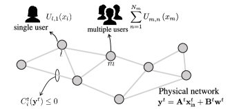
Figure 1: We consider a network of systems, coupled through physical or operational dependencies, where each system is shared by (and affects) a number of users.

Generally, one prerequisite for solving these problems is that the user-specific functions are known or properly crafted based on synthetic or average models. Instead, we consider a case where synthetic costs are not representative of the preferences of individual users, or fail to capture the diversity in their perception of comfort, safety, or dissatisfaction [7, 8, 9]. More precisely, a learning method that leverage human feedback is explored in [7], where a robot observes data in the form of state-action and the discrete dynamics are learned during the execution of the algorithm. An example of field research of occupant satisfaction to the indoor temperature via recording of smiley-face polling station is presented in [8]. Moreover, [9] presents an overview of opportunities and risks of data-driven decision-making methods.

We tackle the problem of solving a network optimization problem when the users’ cost functions are unknown, and develop an online algorithm where the cost functions are learned concurrently with the execution of the algorithmic steps. In particular, the learning procedure leverages “users’ feedback”, and utilizes learning tools from shape-constrained Gaussian Processes (GPs) [10]. The algorithm is implemented in a distributed fashion; this allows users sharing a system to agree on a solution that minimizes the sum of their (learned) functions, without revealing their preferences or their feedback. In this work, we consider the case where the users report their preferences trustworthy (and we do not consider adversarial behaviors). In addition to the feedback from the users, the algorithm leverages the ideas from, e.g., [11, 12], and utilizes measurements of network outputs instead of the network model.

The endeavors are motivated by a number of problems arising in power systems [13, 14, 11], charging of electric vehicles [15], and human-aware robot systems [16], just to name a few. While Section II will explain some examples, we stress here that an accurate model of the comfort/satisfaction level of users is typically unknown, and it may vary not only across individuals, but also for the same individual [7, 8]. In this context, shape-constrained GP is a powerful tool for nonparametric function estimation when the underlying function is presumed to be convex or monotonic [10]; this implies that each user has a preference for a set of solutions.

Contributions. Overall, the main contributions of the paper are as follows. C1) We show how to estimate the users’ functions via GPs and in particular, how to handle asynchronous and noisy data easily. C2) We develop an online algorithm based on a primal-dual method to solve the formulated time-varying network optimization problem; the algorithm is implemented online, and it is modified to accommodate measurements and learned functions. C3) We propose a consensus-based formulation that leads to a distributed online algorithm where users minimize the sum of their (learned) functions, without revealing their preferences or their feedback. C4) For the performance analysis, we view the algorithm as an inexact online primal-dual method where errors are due to the shape-constrained GP approximation and errors in the computation of the gradient of the GP. We derive bounds for a dynamic extension of the network regret [17, 18], and for the average constraint violation (see also, e.g., [19, 20, 21, 22] and references therein for other notions of dynamic regret). And, C5) we showcase the proposed methodology in an example related to control of distributed energy resources in power grids [14].

Prior works. In the context of bandit optimization, a static regret analysis is performed in [19], where the objective is to minimize a sequence of unknown convex cost functions and one has access to functional evaluations. Time-varying cost and constraints are considered in the context of a bandit setting in [23] and online saddle-point algorithms are utilized, where the gradient information is acquired via one-point or multi-point estimates. In [24], a gradient-free approach is presented to solve a multi-agent distributed constrained optimization problem where the goal is to cooperatively minimize the sum of time-changing local cost functions subject to time-varying coupled constraints. As an example of works in the context of zeroth-order methods, a multi-agent optimization problem is analyzed in [25] where the objective is to minimize the average of the nonconvex local costs that depends on the joint actions of the agents. See also [26] for an overview of zeroth-order algorithms. Our approach is different from zeroth-order or bandit methods [23, 19, 26, 25, 24]; these would require multiple functional evaluations at each step to estimate the gradient of the users’ costs – something not feasible for our problem. Our contribution is to use shape-constrained GPs to process feedback that is provided parsimoniously and at irregular intervals. The considered setting is also different from [27], where GPs are utilized to maximize an unknown function.

A similar problem setup was studied in [28]; however, no constraints are considered (in fact, a gradient tracking scheme is utilized) and the user’s cost is assumed to have a known quadratic structure a priori. We significantly extend our previous works [29, 30] by considering a distributed setting and constrained problems. Relative to the works [17, 18] on distributed online primal-dual algorithms, we consider problems where the optimal solution set changes in time (and it is not fixed in time), and with both consensus constraints and time-varying constraints that capture operational limits of the network. We also analyze the network regret when the online algorithm is inexact. Indeed, we can recover an asymptotic bound of 𝒪(T12)𝒪superscript𝑇12{\mathcal{O}}(T^{\frac{1}{2}}) as in [17, 18] from our regret bound when the cost functions are known, the gradients are computed exactly, and the optimal solutions are not time-varying (with T𝑇T the number of time steps). Our analysis can also be utilized to extend [25] to time-varying settings. Finally, we extend the findings of [12, 11] by considering consensus constraints (and accompanying distributed implementations), and by including shape-constrained GPs in the overall algorithmic framework.

The remainder of this paper is organized as follows. Section II presents the time-varying problem, and Section III outlines the GP-based learning approach and the proposed online algorithm. Section IV presents the performance analysis. The numerical results for a demand response problem are in Section V, and Section VI concludes the paper111Notation: Upper-case (lower-case) boldface letters will be used for matrices (column vectors); ()superscripttop(\cdot)^{\top} denotes transposition. For a given column vector 𝐱n𝐱superscript𝑛{\mathbf{x}}\in{\mathbb{R}}^{n}, 𝐱:=𝐱𝐱assigndelimited-∥∥𝐱superscript𝐱top𝐱\lVert{\mathbf{x}}\rVert:=\sqrt{{\mathbf{x}}^{\top}{\mathbf{x}}}; we denote with 𝟏1\mathbf{1} and 𝟎0\mathbf{0} the vectors of all ones and zeros, respectively, where the dimension will be clear from the context. 𝒪()𝒪\mathcal{O}(\cdot) refers to the big-O notation, whereas o()𝑜o(\cdot) refers to the little-o notation. The max operator is defined as [x]+:=max{0,x}assignsuperscriptdelimited-[]𝑥0𝑥[x]^{+}:=\max\{0,x\}. The diameter of 𝒳tsuperscript𝒳𝑡{\mathcal{X}}^{t} is defined as diam(𝒳t)=max{𝐱𝐱:𝐱,𝐱𝒳t}diamsuperscript𝒳𝑡:norm𝐱superscript𝐱𝐱superscript𝐱superscript𝒳𝑡\mathrm{diam}({\mathcal{X}}^{t})=\max\{\|{\mathbf{x}}-{\mathbf{x}}^{\prime}\|\,:\,{\mathbf{x}},{\mathbf{x}}^{\prime}\in{\mathcal{X}}^{t}\}. For a given random variable ξ𝜉\xi\in\mathbb{R}, 𝔼[ξ]𝔼delimited-[]𝜉{\mathbb{E}}[\xi] denotes the expected value of ξ𝜉\xi..

II Problem Statement

We consider a network of M𝑀M systems or devices, with each system interacting with (or shared by) a number of users as illustrated in Figure 1. In particular, we denote by 𝒩m={1,,Nm}subscript𝒩𝑚1subscript𝑁𝑚{\mathcal{N}}_{m}=\{1,\dots,N_{m}\} the set of Nm1subscript𝑁𝑚1N_{m}\geq 1 users interacting with the m𝑚mth system. The steady-state input-output relationship of the network is modeled through the time-varying map

𝐲t=𝐀t𝐱int+𝐁t𝐰tsuperscript𝐲𝑡superscript𝐀𝑡subscriptsuperscript𝐱𝑡insuperscript𝐁𝑡superscript𝐰𝑡{\mathbf{y}}^{t}={\mathbf{A}}^{t}{\mathbf{x}}^{t}_{\textrm{in}}+{\mathbf{B}}^{t}{\mathbf{w}}^{t} (1)

where t𝑡t is the time index; 𝐱int:=[x1t,,xMt]assignsuperscriptsubscript𝐱in𝑡superscriptsuperscriptsubscript𝑥1𝑡superscriptsubscript𝑥𝑀𝑡top{\mathbf{x}}_{\textrm{in}}^{t}:=[x_{1}^{t},\ldots,x_{M}^{t}]^{\top}, with xmtsubscriptsuperscript𝑥𝑡𝑚x^{t}_{m}\in\mathbb{R} the controllable input of the m𝑚mth system; 𝐲tYsuperscript𝐲𝑡superscript𝑌{\mathbf{y}}^{t}\in\mathbb{R}^{Y} is a vector of observables or outputs of the network; 𝐰tWsuperscript𝐰𝑡superscript𝑊{\mathbf{w}}^{t}\in\mathbb{R}^{W} is a vector of unknown exogenous inputs; and, 𝐀tsuperscript𝐀𝑡\mathbf{A}^{t} and 𝐁tsuperscript𝐁𝑡\mathbf{B}^{t} are possibly time-varying matrices (with 𝐀tsuperscript𝐀𝑡{\mathbf{A}}^{t} known and 𝐀t𝟎superscript𝐀𝑡0{\mathbf{A}}^{t}\neq\mathbf{0}) of appropriate dimensions. We assume that t𝒯:={kΔ,k}𝑡𝒯assign𝑘Δ𝑘t\in{\mathcal{T}}:=\{k\Delta,k\in{\mathbb{N}}\}, where Δ>0Δ0\Delta>0 is a given time interval.

Let Um,n::subscript𝑈𝑚𝑛U_{m,n}:\mathbb{R}\rightarrow\mathbb{R} be a convex function representing the cost of a user n𝒩m𝑛subscript𝒩𝑚n\in{\mathcal{N}}_{m} associate with the m𝑚mth device222 We note that the problem formulation and solution approach proposed in this paper can be naturally extended to the case where the number of users interacting with a device changes over time.; this function can capture a sense of dissatisfaction, discomfort, or simply preferences depending on the specific application (a few examples will be provided shortly). The goal is then to compute the sequence of inputs that solves the following time-varying optimization problem [3, 4, 5] associated with the network:

min{xm𝒳mt}m=1Msuperscriptsubscriptsubscript𝑥𝑚superscriptsubscript𝒳𝑚𝑡𝑚1𝑀\displaystyle\underset{\{x_{m}\in{\mathcal{X}}_{m}^{t}\}_{m=1}^{M}}{\min} m=1Mn=1NmUm,n(xm)superscriptsubscript𝑚1𝑀superscriptsubscript𝑛1subscript𝑁𝑚subscript𝑈𝑚𝑛subscript𝑥𝑚\displaystyle\quad\sum_{m=1}^{M}\sum_{n=1}^{N_{m}}U_{m,n}\left(x_{m}\right) (2a)
s. to: Cit(𝐀t𝐱in+𝐁t𝐰t)0,i=1,,NCformulae-sequencesubscriptsuperscript𝐶𝑡𝑖superscript𝐀𝑡subscript𝐱insuperscript𝐁𝑡superscript𝐰𝑡0𝑖1subscript𝑁𝐶\displaystyle C^{t}_{i}\left({\mathbf{A}}^{t}{\mathbf{x}}_{\textrm{in}}+{\mathbf{B}}^{t}{\mathbf{w}}^{t}\right)\leq 0,i=1,\dots,N_{C} (2b)

where {𝒳mt}m=1Msuperscriptsubscriptsuperscriptsubscript𝒳𝑚𝑡𝑚1𝑀\{{\mathcal{X}}_{m}^{t}\}_{m=1}^{M} are time-varying convex and compact sets for the inputs, and Cit:M:subscriptsuperscript𝐶𝑡𝑖superscript𝑀C^{t}_{i}:{\mathbb{R}}^{M}\rightarrow{\mathbb{R}} is a time-varying function parameterized by 𝐰tsuperscript𝐰𝑡{\mathbf{w}}^{t}. In particular, (2b) models operational constraints associated with the network output 𝐲tsuperscript𝐲𝑡{\mathbf{y}}^{t}. The main goal of (2) is to generate a sequence of inputs that minimizes the cost of the users, while respecting pertinent network constraints. To this end, this paper focuses on addressing the following four main challenges related to (2):

\bullet Challenge 1: The variable xmsubscript𝑥𝑚x_{m} is coupled across the users 𝒩msubscript𝒩𝑚{\mathcal{N}}_{m}. Our goal is to solve (2) in a distributed fashion, where users are not required to share information about their costs {Um,n}subscript𝑈𝑚𝑛\{U_{m,n}\} (and their functional evaluations) with the device or the network operator.

\bullet Challenge 2: The costs {Um,n}subscript𝑈𝑚𝑛\{U_{m,n}\} are unknown. One may utilize synthetic cost functions for users’ preferences, comfort or satisfaction based on statistical models; however, these synthetic costs may fail to capture the diversity in the users’ perception, preferences, and goals.

\bullet Challenge 3: The exogenous inputs 𝐰tsuperscript𝐰𝑡{\mathbf{w}}^{t} may be unknown or partially known.

\bullet Challenge 4: The constraints Citsuperscriptsubscript𝐶𝑖𝑡C_{i}^{t} and the sets {𝒳mt}superscriptsubscript𝒳𝑚𝑡\{{\mathcal{X}}_{m}^{t}\} may change at each time t𝑡t; the interval ΔΔ\Delta may not be sufficient to solve each instance of the time-varying problem (2) to convergence.

To address the challenges 1-4 above, this paper will develop a consensus-based online algorithm where the cost functions of the users are learned concurrently with the execution of the algorithm, and measurements of 𝐲tsuperscript𝐲𝑡{\mathbf{y}}^{t} are utilized in the algorithmic updates.

Before proceeding, we list representative examples of applications in networked systems in which the problem (2) and the accompanying online optimization framework considered in this paper are particularly well-suited.

Example 1 (Power grids). In the context of power grids, (2) may capture a demand response task [13, 14] or a real-time optimal power flow problem [11]. In this case, 𝐱insubscript𝐱in{\mathbf{x}}_{\textrm{in}} are the power setpoints of distributed energy resources, 𝐰tsuperscript𝐰𝑡{\mathbf{w}}^{t} is a vector of powers consumed by uncontrollable loads, and ytsuperscript𝑦𝑡y^{t} may represent the total power as yt=𝟏𝐱in+𝟏𝐰tsuperscript𝑦𝑡superscript1topsubscript𝐱insuperscript1topsuperscript𝐰𝑡y^{t}=\mathbf{1}^{\top}{\mathbf{x}}_{\textrm{in}}+\mathbf{1}^{\top}{\mathbf{w}}^{t} and/or voltage magnitudes (one can also compute the matrix 𝐀tsuperscript𝐀𝑡\mathbf{A}^{t} based on a linearized AC model). Constraints (2b) may ensure that the net power follows a given automatic gain control or demand response signal; e.g., Cit(y)=(yyreft)2ζsuperscriptsubscript𝐶𝑖𝑡𝑦superscript𝑦superscriptsubscript𝑦ref𝑡2𝜁C_{i}^{t}(y)=(y-y_{\textrm{ref}}^{t})^{2}-\zeta, where yreftsuperscriptsubscript𝑦ref𝑡y_{\textrm{ref}}^{t} is a given reference signal and ζ>0𝜁0\zeta>0 is an error tolerance. One may also have voltage constraints. The costs {Um,n}subscript𝑈𝑚𝑛\{U_{m,n}\} model discomfort, e.g., the indoor temperature. The number of users depends on the particular setting, for example one may expect a large number of users sharing a conference room in an office building. The users that share a device m𝑚m agrees on the input xmsubscript𝑥𝑚x_{m}; for example, people sharing a room agree on a temperature and, thus, on the use of an HVAC system. \Box

Example 2 (Electric vehicle (EV) charging). The formulation (2) may represent the problem of charging a fleet of vehicles at a charging station; the variable xmsubscript𝑥𝑚x_{m} represents the charging rate (or the expected time for full charging) of a vehicle, constraint (2b) captures limits on the total power consumed by the charging station, while {Um,n}subscript𝑈𝑚𝑛\{U_{m,n}\} capture the dissatisfaction for a given expected time of charging completion [15]. If a EV is shared by multiple users, xmsubscript𝑥𝑚x_{m} represents the agreed expected charging time xmsubscript𝑥𝑚x_{m}. \Box

Additional examples in transportation systems, communication systems, and human-aware robot systems are not included for space limitations.

We now proceed with the reformulation of (2) into a consensus-based problem. To this end, let xm,nsubscript𝑥𝑚𝑛x_{m,n} be an auxiliary variable representing the input for the m𝑚mth system preferred by user n𝒩m𝑛subscript𝒩𝑚n\in{\mathcal{N}}_{m}; with the auxiliary variables in place, stack the optimization variables in the column vector

𝐱t=[x1t,x1,1t,,x1,N1t,,xMt,xM,1t,,xM,NMt].superscript𝐱𝑡superscriptsuperscriptsubscript𝑥1𝑡superscriptsubscript𝑥11𝑡superscriptsubscript𝑥1subscript𝑁1𝑡superscriptsubscript𝑥𝑀𝑡superscriptsubscript𝑥𝑀1𝑡superscriptsubscript𝑥𝑀subscript𝑁𝑀𝑡top{\mathbf{x}}^{t}=\left[x_{1}^{t},x_{1,1}^{t},\dots,x_{1,N_{1}}^{t},\dots,x_{M}^{t},x_{M,1}^{t},\dots,x_{M,N_{M}}^{t}\right]^{\top}.

Accordingly, (1) can be rewritten as 𝐲t=𝐀¯t𝐱t+𝐁t𝐰tsuperscript𝐲𝑡superscript¯𝐀𝑡superscript𝐱𝑡superscript𝐁𝑡superscript𝐰𝑡{\mathbf{y}}^{t}=\bar{{\mathbf{A}}}^{t}{\mathbf{x}}^{t}+{\mathbf{B}}^{t}{\mathbf{w}}^{t}, where 𝐀¯tsuperscript¯𝐀𝑡\bar{{\mathbf{A}}}^{t} is an augmented version of 𝐀tsuperscript𝐀𝑡{\mathbf{A}}^{t} with appropriate zero entries.

Then, (2) can be equivalently reformulated as:

min{xm,xm,n𝒳mt}subscript𝑥𝑚subscript𝑥𝑚𝑛superscriptsubscript𝒳𝑚𝑡\displaystyle\underset{\{x_{m},\,x_{m,n}\in{\mathcal{X}}_{m}^{t}\}}{\min} m=1Mn=1NmUm,n(xm,n)superscriptsubscript𝑚1𝑀superscriptsubscript𝑛1subscript𝑁𝑚subscript𝑈𝑚𝑛subscript𝑥𝑚𝑛\displaystyle\quad\sum_{m=1}^{M}\sum_{n=1}^{N_{m}}U_{m,n}\left(x_{m,n}\right) (3a)
s. to: Cit(𝐀¯t𝐱+𝐁t𝐰t)0,i=1,,NCformulae-sequences. to: subscriptsuperscript𝐶𝑡𝑖superscript¯𝐀𝑡𝐱superscript𝐁𝑡superscript𝐰𝑡0𝑖1subscript𝑁𝐶\displaystyle\text{s. to: }C^{t}_{i}\left(\bar{{\mathbf{A}}}^{t}{\mathbf{x}}+{\mathbf{B}}^{t}{\mathbf{w}}^{t}\right)\leq 0,i=1,\dots,N_{C} (3b)
xm=xm,n,n𝒩m,m=1,,Mformulae-sequencesubscript𝑥𝑚subscript𝑥𝑚𝑛formulae-sequencefor-all𝑛subscript𝒩𝑚for-all𝑚1𝑀\displaystyle x_{m}=x_{m,n},\,\forall\,n\in{\mathcal{N}}_{m},\,\forall\,m=1,\dots,M (3c)

where (3c) defines consensus constraints for the m𝑚mth system and its users. We note that the choice of posing the consensus constraints as in (3c) is not generic; the particular structure of (3c), which can be modeled as a star graph (with the system as the central node) will facilitate the development of a closed-loop algorithm where {xm}subscript𝑥𝑚\{x_{m}\} will be physical inputs (as in (1)) and {xm,n}subscript𝑥𝑚𝑛\{x_{m,n}\} will be auxiliary control variables.

For future developments, define f(𝐱):=m=1Mn=1NmUm,n(xm,n)assign𝑓𝐱superscriptsubscript𝑚1𝑀superscriptsubscript𝑛1subscript𝑁𝑚subscript𝑈𝑚𝑛subscript𝑥𝑚𝑛f({\mathbf{x}}):=\sum_{m=1}^{M}\sum_{n=1}^{N_{m}}U_{m,n}\left(x_{m,n}\right) and 𝒳t:=𝒳1t××𝒳MtMassignsuperscript𝒳𝑡subscriptsuperscript𝒳𝑡1subscriptsuperscript𝒳𝑡𝑀superscript𝑀\mathcal{X}^{t}:=\mathcal{X}^{t}_{1}\times\dots\times\mathcal{X}^{t}_{M}\subseteq{\mathbb{R}}^{M}. For each device m𝑚m, define the incidence matrix 𝐃mNm×(1+Nm)subscript𝐃𝑚superscriptsubscript𝑁𝑚1subscript𝑁𝑚{\mathbf{D}}_{m}\in{\mathbb{R}}^{N_{m}\times(1+N_{m})}, which represents the relation between the device and the users sharing that device. For example, if the device 111 is shared by 2 users we have that

𝐃1=[110101].subscript𝐃1matrix110101{\mathbf{D}}_{1}=\begin{bmatrix}1&-1&0\\ 1&0&-1\end{bmatrix}.

By organizing these incidence matrices in a block diagonal matrix, we construct the augmented incidence matrix 𝐃=diag(𝐃1,𝐃2,,𝐃M)𝐃diagsubscript𝐃1subscript𝐃2subscript𝐃𝑀{\mathbf{D}}=\mathrm{diag}({\mathbf{D}}_{1},{\mathbf{D}}_{2},\dots,{\mathbf{D}}_{M}). Then, (3c) can be compactly written as 𝐃𝐱=𝟎𝐃𝐱0{\mathbf{D}}{\mathbf{x}}=\mathbf{0}, capturing consensus constraints over M𝑀M systems.

The next section outlines the proposed algorithm to solve the time-varying network optimization problem (2). We note that in what follows we consider the case where NC=1subscript𝑁𝐶1N_{C}=1 to simplify exposition and notation; however, the technical arguments of this paper straightforwardly extend to problems with multiple constraints on 𝐲tsuperscript𝐲𝑡{\mathbf{y}}^{t}.

III Distributed Online Algorithm

In this section, we present our consensus-based online algorithm for solving (3). We first explain how to derive a distributed online algorithm based on a primal-dual method; then, we elaborate on how to estimate the cost functions based on feedback received from the users at infrequent times.

III-A Online primal-dual algorithm

We start by defining the time-varying Lagrangian function associated with (3) as follows:

t(𝐱t,νt,𝝀t):=assignsuperscript𝑡superscript𝐱𝑡superscript𝜈𝑡superscript𝝀𝑡absent\displaystyle{\mathcal{L}}^{t}({\mathbf{x}}^{t},\nu^{t},{\mbox{\boldmath$\lambda$}}^{t}):= f(𝐱t)+νtCt(𝐀¯t𝐱t+𝐁t𝐰t)+(𝐃𝐱t)𝝀t𝑓superscript𝐱𝑡superscript𝜈𝑡superscript𝐶𝑡superscript¯𝐀𝑡superscript𝐱𝑡superscript𝐁𝑡superscript𝐰𝑡superscriptsuperscript𝐃𝐱𝑡topsuperscript𝝀𝑡\displaystyle f({\mathbf{x}}^{t})+\nu^{t}\,C^{t}\left(\bar{{\mathbf{A}}}^{t}{\mathbf{x}}^{t}+{\mathbf{B}}^{t}{\mathbf{w}}^{t}\right)+({\mathbf{D}}{\mathbf{x}}^{t})^{\top}{\mbox{\boldmath$\lambda$}}^{t}

where νt+superscript𝜈𝑡subscript\nu^{t}\in{\mathbb{R}}_{+}, 𝝀tNsuperscript𝝀𝑡superscript𝑁{\mbox{\boldmath$\lambda$}}^{t}\in{\mathbb{R}}^{N} are the dual variables associated with the constraint (3b), and the M𝑀M consensus constraints (3c), respectively.

Recall that t𝒯:={kΔ,k}𝑡𝒯assign𝑘Δ𝑘t\in{\mathcal{T}}:=\{k\Delta,k\in{\mathbb{N}}\}, where Δ>0Δ0\Delta>0 represents the time required to perform one step of the online algorithm (and with the constraints and the vector 𝐰tsuperscript𝐰𝑡{\mathbf{w}}^{t} possibly changing at every interval ΔΔ\Delta). For a given step size α>0𝛼0\alpha>0, a model-based online projected primal-dual algorithm involves the sequential execution of the following steps:

𝐱t+1superscript𝐱𝑡1\displaystyle{\mathbf{x}}^{t+1} =proj𝒳t{𝐱tα(𝐱f(𝐱t)\displaystyle=\mathrm{proj}_{{{\mathcal{X}}^{t}}}\left\{{\mathbf{x}}^{t}-\alpha\left(\nabla_{{\mathbf{x}}}f({\mathbf{x}}^{t})\right.\right.
+νt(𝐀¯t)𝐱Ct(𝐀¯t𝐱t+𝐁t𝐰t)+𝐃𝝀t)},\displaystyle\left.\left.\,\,\,\,+\nu^{t}(\bar{{\mathbf{A}}}^{t})^{\top}\nabla_{{\mathbf{x}}}C^{t}(\bar{{\mathbf{A}}}^{t}{\mathbf{x}}^{t}+{\mathbf{B}}^{t}{\mathbf{w}}^{t})+{\mathbf{D}}^{\top}{\mbox{\boldmath$\lambda$}}^{t}\right)\right\}, (4a)
νt+1superscript𝜈𝑡1\displaystyle\nu^{t+1} =projΨt{νt+αCt(𝐀¯t𝐱t+𝐁t𝐰t)},absentsubscriptprojsuperscriptΨ𝑡superscript𝜈𝑡𝛼superscript𝐶𝑡superscript¯𝐀𝑡superscript𝐱𝑡superscript𝐁𝑡superscript𝐰𝑡\displaystyle=\mathrm{proj}_{\Psi^{t}}\left\{\nu^{t}+\alpha C^{t}\left(\bar{{\mathbf{A}}}^{t}{\mathbf{x}}^{t}+{\mathbf{B}}^{t}{\mathbf{w}}^{t}\right)\right\}, (4b)
𝝀t+1superscript𝝀𝑡1\displaystyle{\mbox{\boldmath$\lambda$}}^{t+1} =projΛt{𝝀t+α𝐃𝐱t},absentsubscriptprojsuperscriptΛ𝑡superscript𝝀𝑡𝛼superscript𝐃𝐱𝑡\displaystyle=\mathrm{proj}_{{\Lambda^{t}}}\left\{{\mbox{\boldmath$\lambda$}}^{t}+\alpha{\mathbf{D}}{\mathbf{x}}^{t}\right\}, (4c)

where ΨtsuperscriptΨ𝑡\Psi^{t} is a convex and compact set, and Λt=Λ1,1t××Λ1,N1t××ΛM,NMtsuperscriptΛ𝑡superscriptsubscriptΛ11𝑡superscriptsubscriptΛ1subscript𝑁1𝑡superscriptsubscriptΛ𝑀subscript𝑁𝑀𝑡\Lambda^{t}=\Lambda_{1,1}^{t}\times\dots\times\Lambda_{1,N_{1}}^{t}\times\dots\times\Lambda_{M,N_{M}}^{t}, with Λm,ntsuperscriptsubscriptΛ𝑚𝑛𝑡\Lambda_{m,n}^{t} also a convex and compact set constructed as explained shortly in Section IV (and in, e.g., [1] and [17]).

We note that the steps (4a) and (4b) require one to know 𝐰tsuperscript𝐰𝑡{\mathbf{w}}^{t} and 𝐁tsuperscript𝐁𝑡{\mathbf{B}}^{t} (as explained in Challenges 3 and 4). To bypass this hurdle, we adopt the strategy proposed in, e.g., [11, 12]. To this end, assume that 𝐱intsuperscriptsubscript𝐱in𝑡{\mathbf{x}}_{\mathrm{in}}^{t} are implemented as inputs to the systems at time t𝑡t, and let 𝐲^tsuperscript^𝐲𝑡\hat{{\mathbf{y}}}^{t} represent a measurement of 𝐲tsuperscript𝐲𝑡{\mathbf{y}}^{t} collected at time t𝑡t. Then, νt+1superscript𝜈𝑡1\nu^{t+1} can be computed as νt+1=projΨ{νt+αCt(𝐲^t)}superscript𝜈𝑡1subscriptprojΨsuperscript𝜈𝑡𝛼superscript𝐶𝑡superscript^𝐲𝑡\nu^{t+1}=\mathrm{proj}_{\Psi}\left\{\nu^{t}+\alpha C^{t}\left(\hat{{\mathbf{y}}}^{t}\right)\right\}; it is clear that information about 𝐰tsuperscript𝐰𝑡{\mathbf{w}}^{t} and 𝐁tsuperscript𝐁𝑡{\mathbf{B}}^{t} is not required in this case. We also note that the step (4a) would require the gradient of the functions {Um,n}subscript𝑈𝑚𝑛\{U_{m,n}\}, which are not known (see Challenge 1). Let U^m,nt(xmt)subscriptsuperscript^𝑈𝑡𝑚𝑛subscriptsuperscript𝑥𝑡𝑚\hat{U}^{t}_{m,n}(x^{t}_{m}) represent an estimate of the function Um,n(xmt)subscript𝑈𝑚𝑛subscriptsuperscript𝑥𝑡𝑚U_{m,n}(x^{t}_{m}) available at xmtsubscriptsuperscript𝑥𝑡𝑚x^{t}_{m}, and let gm,ntsuperscriptsubscript𝑔𝑚𝑛𝑡g_{m,n}^{t} denote an estimate of the gradient (or derivative, in this case) of Um,n(xmt)subscript𝑈𝑚𝑛subscriptsuperscript𝑥𝑡𝑚U_{m,n}(x^{t}_{m}) at time t𝑡t. With these definitions, the steps in (4) can be suitably modified to accommodate measurements of 𝐲tsuperscript𝐲𝑡{\mathbf{y}}^{t} and estimates of the gradient of the cost function:

xmt+1superscriptsubscript𝑥𝑚𝑡1\displaystyle x_{m}^{t+1} =proj𝒳mt{xmtα(νt(𝐚mt)Ct(𝐲^t)+n=1Nmλm,nt)}absentsubscriptprojsuperscriptsubscript𝒳𝑚𝑡superscriptsubscript𝑥𝑚𝑡𝛼superscript𝜈𝑡superscriptsuperscriptsubscript𝐚𝑚𝑡topsuperscript𝐶𝑡superscript^𝐲𝑡superscriptsubscript𝑛1subscript𝑁𝑚subscriptsuperscript𝜆𝑡𝑚𝑛\displaystyle=\mathrm{proj}_{{{\mathcal{X}}_{m}^{t}}}\left\{x_{m}^{t}-\alpha\left(\nu^{t}({\mathbf{a}}_{m}^{t})^{\top}\nabla C^{t}(\hat{{\mathbf{y}}}^{t})+\sum_{n=1}^{N_{m}}\lambda^{t}_{m,n}\right)\right\} (5a)
xm,nt+1superscriptsubscript𝑥𝑚𝑛𝑡1\displaystyle x_{m,n}^{t+1} =proj𝒳mt{xm,ntα(gm,ntλm,nt)}n𝒩m,m,formulae-sequenceabsentsubscriptprojsuperscriptsubscript𝒳𝑚𝑡superscriptsubscript𝑥𝑚𝑛𝑡𝛼superscriptsubscript𝑔𝑚𝑛𝑡subscriptsuperscript𝜆𝑡𝑚𝑛for-all𝑛subscript𝒩𝑚for-all𝑚\displaystyle=\mathrm{proj}_{{{\mathcal{X}}_{m}^{t}}}\left\{x_{m,n}^{t}-\alpha\left(g_{m,n}^{t}-\lambda^{t}_{m,n}\right)\right\}\;\forall\,n\in{\mathcal{N}}_{m},\,\forall\,m, (5b)
νt+1superscript𝜈𝑡1\displaystyle\nu^{t+1} =projΨt{νt+αCt(𝐲^t)},absentsubscriptprojsuperscriptΨ𝑡superscript𝜈𝑡𝛼superscript𝐶𝑡superscript^𝐲𝑡\displaystyle=\mathrm{proj}_{\Psi^{t}}\left\{\nu^{t}+\alpha C^{t}\left(\hat{{\mathbf{y}}}^{t}\right)\right\}, (5c)
λm,nt+1superscriptsubscript𝜆𝑚𝑛𝑡1\displaystyle\lambda_{m,n}^{t+1} =projΛm,nt{λm,nt+α(xmtxm,nt)},n𝒩m,m,formulae-sequenceabsentsubscriptprojsuperscriptsubscriptΛ𝑚𝑛𝑡superscriptsubscript𝜆𝑚𝑛𝑡𝛼superscriptsubscript𝑥𝑚𝑡superscriptsubscript𝑥𝑚𝑛𝑡for-all𝑛subscript𝒩𝑚for-all𝑚\displaystyle=\mathrm{proj}_{{\Lambda_{m,n}^{t}}}\left\{\lambda_{m,n}^{t}+\alpha\left(x_{m}^{t}-x_{m,n}^{t}\right)\right\},\forall\,n\in{\mathcal{N}}_{m},\,\forall\,m, (5d)

where 𝐚mtsuperscriptsubscript𝐚𝑚𝑡{\mathbf{a}}_{m}^{t} is the m𝑚mth column of the matrix 𝐀tsuperscript𝐀𝑡{\mathbf{A}}^{t}, and we note that step (5a) is performed in parallel at each system. While measurements of 𝐲tsuperscript𝐲𝑡{\mathbf{y}}^{t} are utilized in the primal step (5a) and in the dual step (5c), an estimate of the gradient gm,ntsuperscriptsubscript𝑔𝑚𝑛𝑡g_{m,n}^{t} will be obtained by leveraging feedback from the users as explained in the following subsection. Subsequently, Section III-C will overview the steps of the proposed algorithm.

III-B Online Learning via Shape-Constrained GPs

We assume that the feedback of the user comes in the form of a (possibly noisy) functional evaluation; that is, for a given point x𝑥x, one may receive from a user n𝑛n interacting with the device m𝑚m a rating z𝑧z given by z=Um,n(x)+ϵ𝑧subscript𝑈𝑚𝑛𝑥italic-ϵz=U_{m,n}(x)+\epsilon. With this model, a popular way to obtain the gradient of Um,nsubscript𝑈𝑚𝑛U_{m,n} at a point x𝑥x is via zeroth-order methods (see, e.g., [23, 26] and references therein). However, zeroth-order methods are not well-suited for our algorithm, because they would require feedback from each individual user at each iteration of the algorithm (either a single functional evaluation or more, depending on the particular method utilized). Instead, we consider a more realistic case where users may provide feedback more parsimoniously and at irregular intervals.

With this setting in mind, we consider utilizing the noisy functional evaluations provided by a user to estimate the function Um,nsubscript𝑈𝑚𝑛U_{m,n} via GPs [31]. In particular, we apply a GP with specific constraints on the shape of the function. As explained in [10], shape-constrained GPs offers a powerful tool for nonparametric function estimation when the underlying function is presumed to be convex or monotonic. In our case, convexity or monotonicity implies that each user has a preference for a particular solution (or a convex set of solutions), and the dissatisfaction or discomfort increases as the system deviates from such a preferred point. In the following, we first briefly introduce GPs, and then we provide the main equations to estimate Um,nsubscript𝑈𝑚𝑛U_{m,n} via a shape-constrained GPs. Since we utilize a GP per function Um,nsubscript𝑈𝑚𝑛U_{m,n}, we drop the subscripts m𝑚m, n𝑛n for simplicity of exposition. We also note that the extension to the multi-dimensional shape-constrained GP is possible (see, for example, [10]); however, it is left as future work.

A GP is a stochastic process U(x)𝑈𝑥U(x) and it is specified by its mean function μ(x)𝜇𝑥\mu({x}) and its covariance function k(x,x)𝑘𝑥superscript𝑥k(x,x^{\prime}); where k(,)𝑘k(\cdot,\cdot) is a given kernel; i.e., for any x,x𝒳𝑥superscript𝑥𝒳x,x^{\prime}\in\mathcal{X}\subseteq\mathbb{R}, μ(x)=𝔼[U(x)]𝜇𝑥𝔼delimited-[]𝑈𝑥\mu({x})=\mathbb{E}[U({x})] and k(x,x)=𝔼[(U(x)μ(x))(U(x)μ(x))]𝑘𝑥superscript𝑥𝔼delimited-[]𝑈𝑥𝜇𝑥𝑈superscript𝑥𝜇superscript𝑥k({x},{x}^{\prime})=\mathbb{E}[(U({x})-\mu({x}))(U({x}^{\prime})-\mu({x}^{\prime}))] [31]. Hereafter, we use the short-hand notation U(x)𝒢𝒫(μ(x),k(x,x))similar-to𝑈𝑥𝒢𝒫𝜇𝑥𝑘𝑥superscript𝑥U(x)\sim\mathcal{GP}(\mu(x),k(x,x^{\prime})) for U(x)𝑈𝑥U({x}) defined as a GP with mean μ(x)𝜇𝑥\mu(x) and covariance k(x,x)𝑘𝑥superscript𝑥k(x,x^{\prime}). Let 𝐱p=[x1𝒳,,xp𝒳]subscript𝐱𝑝superscriptdelimited-[]formulae-sequencesubscript𝑥1𝒳subscript𝑥𝑝𝒳top\mathbf{x}_{p}=[x_{1}\in\mathcal{X},\dots,x_{p}\in\mathcal{X}]^{\top} be the set of p𝑝p sample points collected over a given period333In the context of our work, the vector 𝐱psubscript𝐱𝑝\mathbf{x}_{p} associated with a system m𝑚m and a user n𝑛n would contain the points xm,nt1,,xm,ntpsuperscriptsubscript𝑥𝑚𝑛subscript𝑡1superscriptsubscript𝑥𝑚𝑛subscript𝑡𝑝x_{m,n}^{t_{1}},\ldots,x_{m,n}^{t_{p}}, where {ti}i=1p𝒯superscriptsubscriptsubscript𝑡𝑖𝑖1𝑝𝒯\{t_{i}\}_{i=1}^{p}\subset\mathcal{T} are the times instants where the user provides feedback.; let zi=U(xi)+ϵisubscript𝑧𝑖𝑈subscript𝑥𝑖subscriptitalic-ϵ𝑖{z}_{i}=U({x}_{i})+\epsilon_{i}, with ϵiiid𝒩(0,σ2)superscriptsimilar-toiidsubscriptitalic-ϵ𝑖𝒩0superscript𝜎2\epsilon_{i}\stackrel{{\scriptstyle\mathrm{iid}}}{{\sim}}\mathcal{N}({0},\sigma^{2}) Gaussian noise, be the noisy measurement at the sample point xisubscript𝑥𝑖x_{i}; define further 𝐳=[z1,,zp]𝐳superscriptsubscript𝑧1subscript𝑧𝑝top\mathbf{z}=[z_{1},\dots,z_{p}]^{\top}. Then, the posterior distribution of (U(x)|𝐱p,𝐳)conditional𝑈𝑥subscript𝐱𝑝𝐳(U(x)|{\mathbf{x}}_{p},{\mathbf{z}}) is a GP with mean μ(x)𝜇𝑥\mu({x}), covariance k(x,x)𝑘𝑥superscript𝑥k({x},{x}^{\prime}), and variance σ2(x)superscript𝜎2𝑥\sigma^{2}(x) given by [31]:

μ(x)𝜇𝑥\displaystyle\mu({x}) =𝐤(x)(𝐊+σ2𝐈)1𝐳,absent𝐤superscript𝑥topsuperscript𝐊superscript𝜎2𝐈1𝐳\displaystyle=\mathbf{k}(x)^{\top}(\mathbf{K}+\sigma^{2}\mathbf{I})^{-1}\mathbf{z}, (6a)
k(x,x)𝑘𝑥superscript𝑥\displaystyle k({x},{x}^{\prime}) =k(x,x)𝐤(x)(𝐊+σ2𝐈)1𝐤(x),absent𝑘𝑥superscript𝑥𝐤superscript𝑥topsuperscript𝐊superscript𝜎2𝐈1𝐤superscript𝑥\displaystyle=k(x,x^{\prime})-\mathbf{k}(x)^{\top}(\mathbf{K}+\sigma^{2}\mathbf{I})^{-1}\mathbf{k}(x^{\prime}), (6b)
σ2(x)superscript𝜎2𝑥\displaystyle\sigma^{2}(x) =k(x,x),absent𝑘𝑥𝑥\displaystyle=k(x,x), (6c)

where 𝐤(x)=[k(x1,x),,k(xp,x)]𝐤𝑥superscript𝑘subscript𝑥1𝑥𝑘subscript𝑥𝑝𝑥top\mathbf{k}(x)=[k(x_{1},x),\dots,k(x_{p},x)]^{\top}, 𝐊𝐊\mathbf{K} is the positive definite kernel matrix [k(x,x)]delimited-[]𝑘𝑥superscript𝑥[k(x,x^{\prime})]. Note that (6) depends on the p𝑝p sample points for a specific period of time. Thus, an estimate of the unknown function U(x)𝑈𝑥U({x}) can be written as U(x)𝒢𝒫(μ(x),k(x,x))similar-to𝑈𝑥𝒢𝒫𝜇𝑥𝑘𝑥superscript𝑥U({x})\sim\mathcal{GP}(\mu({x}),k({x},{x}^{\prime})). Using a squared exponential (SE) kernel as an example, k(x,x)𝑘𝑥superscript𝑥k({x},{x}^{\prime}) is given by k(x,x)=σf2e122(xx)2𝑘𝑥superscript𝑥superscriptsubscript𝜎𝑓2superscripte12superscript2superscript𝑥superscript𝑥2k({x},{x}^{\prime})=\sigma_{f}^{2}\mathrm{e}^{-\frac{1}{2\ell^{2}}({x}-{x}^{\prime})^{2}} for the univariante input case, where the hyperparameters are the signal variance σf2superscriptsubscript𝜎𝑓2\sigma_{f}^{2} and the characteristic length-scale \ell.

We now explain how to enforce shape constraints through the use of derivative processes (noting that since differentiation is a linear operator, derivatives of a GP remain a GP [31]). Because the GP obtained from the SE kernel function has derivatives of all orders, the mean and covariance function (jointly with the original process and the second-order derivative process) are [10]:

𝔼[2U(x)x2]=2μ(x)x2=0,𝔼delimited-[]superscript2𝑈𝑥superscript𝑥2superscript2𝜇𝑥superscript𝑥20\mathbb{E}\left[\frac{\partial^{2}U({x})}{\partial{x}^{2}}\right]=\frac{\partial^{2}\mu({x})}{\partial{x}^{2}}={0}, (7a)
k22(x,x):=cov[2U(x)x2,2U(x)x2]=σf2e122(xx)2×14(14(xx)4126(xx)2+3),assignsuperscript𝑘22𝑥superscript𝑥covsuperscript2𝑈𝑥superscript𝑥2superscript2𝑈superscript𝑥superscript𝑥2superscriptsubscript𝜎𝑓2superscripte12superscript2superscript𝑥superscript𝑥21superscript41superscript4superscript𝑥superscript𝑥41superscript26superscript𝑥superscript𝑥23k^{22}(x,x^{\prime}):=\text{cov}\left[\frac{\partial^{2}U({x})}{\partial{x}^{2}},\frac{\partial^{2}U({x}^{\prime})}{\partial{x}^{\prime 2}}\right]=\sigma_{f}^{2}\mathrm{e}^{-\frac{1}{2\ell^{2}}(x-x^{\prime})^{2}}\times\\ \frac{1}{\ell^{4}}\left(\frac{1}{\ell^{4}}(x-x^{\prime})^{4}-\frac{1}{\ell^{2}}6(x-x^{\prime})^{2}+3\right), (7b)
k02(x,x):=cov[2U(x)x2,U(x)]=σf2e122(xx)2(14(xx)212).assignsuperscript𝑘02𝑥superscript𝑥covsuperscript2𝑈𝑥superscript𝑥2𝑈superscript𝑥superscriptsubscript𝜎𝑓2superscripte12superscript2superscript𝑥superscript𝑥21superscript4superscript𝑥superscript𝑥21superscript2k^{02}(x,x^{\prime}):=\text{cov}\left[\frac{\partial^{2}U({x})}{\partial{x}^{2}},U({x}^{\prime})\right]\\ =\sigma_{f}^{2}\mathrm{e}^{-\frac{1}{2\ell^{2}}(x-x^{\prime})^{2}}\left(\frac{1}{\ell^{4}}(x-x^{\prime})^{2}-\frac{1}{\ell^{2}}\right). (7c)

We consider enforcing constraints on the second-order derivative at q𝑞q points 𝐬:=[s1,,sq]assign𝐬superscriptsubscript𝑠1subscript𝑠𝑞top\mathbf{s}:=[s_{1},\dots,s_{q}]^{\top} (and these points may be in general different from 𝐱psubscript𝐱𝑝{\mathbf{x}}_{p}). Let 𝐔(𝐱p)=[U(x1),,U(xp)]𝐔subscript𝐱𝑝superscript𝑈subscript𝑥1𝑈subscript𝑥𝑝top\mathbf{U}(\mathbf{x}_{p})=[U(x_{1}),\dots,U(x_{p})]^{\top} and 𝐔′′(𝐬)=[U′′(s1),,U′′(sq)]superscript𝐔′′𝐬superscriptsuperscript𝑈′′subscript𝑠1superscript𝑈′′subscript𝑠𝑞top\mathbf{U}^{\prime\prime}(\mathbf{s})=[U^{\prime\prime}(s_{1}),\dots,U^{\prime\prime}(s_{q})]^{\top}; then, the joint distribution of the GP and its second-order derivative is:

[𝐔(𝐱p)𝐔′′(𝐬)]𝒩([μ𝟏p𝟎q],[𝐊(𝐱p,𝐱p)𝐊𝟎𝟐(𝐱p,𝐬)𝐊𝟐𝟎(𝐬,𝐱p)𝐊𝟐𝟐(𝐬,𝐬)]),similar-tomatrix𝐔subscript𝐱𝑝superscript𝐔′′𝐬𝒩matrix𝜇subscript1𝑝subscript0𝑞matrix𝐊subscript𝐱𝑝subscript𝐱𝑝superscript𝐊02subscript𝐱𝑝𝐬superscript𝐊20𝐬subscript𝐱𝑝superscript𝐊22𝐬𝐬\begin{bmatrix}\mathbf{U}(\mathbf{x}_{p})\\ \mathbf{U}^{\prime\prime}(\mathbf{s})\end{bmatrix}\sim\mathcal{N}\bigg{(}\begin{bmatrix}\mu\mathbf{1}_{p}\\ \mathbf{0}_{q}\end{bmatrix},\begin{bmatrix}\mathbf{K}(\mathbf{x}_{p},\mathbf{x}_{p})&\mathbf{K}^{\mathbf{02}}(\mathbf{x}_{p},\mathbf{s})\\ \mathbf{K}^{\mathbf{20}}(\mathbf{s},\mathbf{x}_{p})&\mathbf{K}^{\mathbf{22}}(\mathbf{s},\mathbf{s})\end{bmatrix}\bigg{)},

where,

𝐊(𝐱p,𝐱p)𝐊subscript𝐱𝑝subscript𝐱𝑝\displaystyle\mathbf{K}(\mathbf{x}_{p},\mathbf{x}_{p}) =𝐊,𝐊𝟎𝟐(𝐱p,𝐬)=[k02(x,s)],formulae-sequenceabsent𝐊superscript𝐊02subscript𝐱𝑝𝐬delimited-[]superscript𝑘02𝑥𝑠\displaystyle=\mathbf{K},\qquad\qquad\qquad\mathbf{K}^{\mathbf{02}}(\mathbf{x}_{p},\mathbf{s})=[k^{02}(x,s)],
𝐊𝟐𝟎(𝐬,𝐱p)superscript𝐊20𝐬subscript𝐱𝑝\displaystyle\mathbf{K}^{\mathbf{20}}(\mathbf{s},\mathbf{x}_{p}) =𝐊𝟎𝟐(𝐱p,𝐬),𝐊𝟐𝟐(𝐬,𝐬)=[k22(s,s)].formulae-sequenceabsentsuperscript𝐊02superscriptsubscript𝐱𝑝𝐬topsuperscript𝐊22𝐬𝐬delimited-[]superscript𝑘22𝑠superscript𝑠\displaystyle=\mathbf{K}^{\mathbf{02}}(\mathbf{x}_{p},\mathbf{s})^{\top},\qquad\;\mathbf{K}^{\mathbf{22}}(\mathbf{s},\mathbf{s})=[k^{22}(s,s^{\prime})].

Next, assign to U()𝑈U(\cdot) a GP prior, and consider aiming at an estimated function that is LUsubscript𝐿𝑈L_{U}-smooth and γUsubscript𝛾𝑈\gamma_{U}-strongly convex, for a given LU>0subscript𝐿𝑈0L_{U}>0 and γU>0subscript𝛾𝑈0\gamma_{U}>0. Then, following [10, Lemma 3.1], the joint conditional posterior distribution of (𝐔(x)|𝐔′′(𝐬),𝐱p,𝐳)conditional𝐔superscript𝑥superscript𝐔′′𝐬subscript𝐱𝑝𝐳(\mathbf{U}({x}^{\circ})|\mathbf{U}^{\prime\prime}(\mathbf{s}),\mathbf{x}_{p},\mathbf{z}), for a point xsuperscript𝑥{x}^{\circ}\in\mathbb{R}, given the current observations 𝐳𝐳\mathbf{z}, is a GP with mean, covariance, and standard deviation given by:

μ¯(x)=μ+B3(𝐱p,x,𝐬)B1(𝐱p,𝐬)1(𝐳μ𝟏p)¯𝜇superscript𝑥𝜇subscript𝐵3subscript𝐱𝑝superscript𝑥𝐬subscript𝐵1superscriptsubscript𝐱𝑝𝐬1𝐳𝜇subscript1𝑝\displaystyle\bar{\mu}({x^{\circ}})=\mu+B_{3}({\mathbf{x}}_{p},{x}^{\circ},\mathbf{s})B_{1}({\mathbf{x}}_{p},\mathbf{s})^{-1}(\mathbf{z}-\mu\mathbf{1}_{p})
+(A2(x,𝐬)B3(𝐱p,x,𝐬)B1(𝐱p,𝐬)1A1(𝐱p,𝐬))𝐔′′(𝐬),subscript𝐴2superscript𝑥𝐬subscript𝐵3subscript𝐱𝑝superscript𝑥𝐬subscript𝐵1superscriptsubscript𝐱𝑝𝐬1subscript𝐴1subscript𝐱𝑝𝐬superscript𝐔′′𝐬\displaystyle+(A_{2}({x}^{\circ},\mathbf{s})-B_{3}({\mathbf{x}}_{p},{x}^{\circ},\mathbf{s})B_{1}({\mathbf{x}}_{p},\mathbf{s})^{-1}A_{1}({\mathbf{x}}_{p},\mathbf{s}))\mathbf{U}^{\prime\prime}(\mathbf{s}), (8a)
k¯(x,x)=A(𝐱p,x,𝐬),¯𝑘superscript𝑥superscriptsuperscript𝑥𝐴subscript𝐱𝑝superscript𝑥𝐬\displaystyle\bar{k}({x^{\circ}},{x^{\circ}}^{\prime})=A({\mathbf{x}}_{p},{x}^{\circ},\mathbf{s}), (8b)
σ¯(x)=A(𝐱p,x,𝐬),¯𝜎superscript𝑥𝐴subscript𝐱𝑝superscript𝑥𝐬\displaystyle\bar{\sigma}(x^{\circ})=\sqrt{A({\mathbf{x}}_{p},{x}^{\circ},\mathbf{s})}, (8c)

and the posterior distribution of (𝐔′′(𝐬)|𝐱p,𝐳)conditionalsuperscript𝐔′′𝐬subscript𝐱𝑝𝐳(\mathbf{U}^{\prime\prime}(\mathbf{s})|\mathbf{x}_{p},\mathbf{z}) is given by:

(𝐔′′(𝐬)|𝐱p,𝐳)𝒩(𝝁(𝐬),𝐒(𝐬,𝐬))𝟏{γUU′′(si)LU,i=1,,q}proportional-toconditionalsuperscript𝐔′′𝐬subscript𝐱𝑝𝐳𝒩𝝁𝐬𝐒𝐬𝐬subscript1formulae-sequencesubscript𝛾𝑈superscript𝑈′′subscript𝑠𝑖subscript𝐿𝑈𝑖1𝑞(\mathbf{U}^{\prime\prime}(\mathbf{s})|\mathbf{x}_{p},\mathbf{z})\propto\mathcal{N}({\mbox{\boldmath$\mu$}}(\mathbf{s}),\mathbf{S}(\mathbf{s},\mathbf{s}))\mathbf{1}_{\{\gamma_{U}\leq U^{\prime\prime}(s_{i})\leq L_{U},\,i=1,\dots,q\}}

where 𝟏{}subscript1\mathbf{1}_{\{\cdot\}} is a set indicator function, (𝐔′′(𝐬)|𝐱p,𝐳)conditionalsuperscript𝐔′′𝐬subscript𝐱𝑝𝐳(\mathbf{U}^{\prime\prime}(\mathbf{s})|\mathbf{x}_{p},\mathbf{z}) is a truncated normal distribution and,

𝝁(𝐬)𝝁𝐬\displaystyle{\mbox{\boldmath$\mu$}}(\mathbf{s}) =𝐊𝟐𝟎(𝐬,𝐱p)(σ2𝐈+𝐊(𝐱p,𝐱p))1(𝐳μ𝟏p),absentsuperscript𝐊20𝐬subscript𝐱𝑝superscriptsuperscript𝜎2𝐈𝐊subscript𝐱𝑝subscript𝐱𝑝1𝐳𝜇subscript1𝑝\displaystyle=\mathbf{K}^{\mathbf{20}}(\mathbf{s},\mathbf{x}_{p})(\sigma^{2}\mathbf{I}+\mathbf{K}(\mathbf{x}_{p},\mathbf{x}_{p}))^{-1}(\mathbf{z}-\mu\mathbf{1}_{p}),
𝐒(𝐬,𝐬)𝐒𝐬𝐬\displaystyle\mathbf{S}(\mathbf{s},\mathbf{s}) =𝐊𝟐𝟐(𝐬,𝐬)absentsuperscript𝐊22𝐬𝐬\displaystyle=\mathbf{K}^{\mathbf{22}}(\mathbf{s},\mathbf{s})
𝐊𝟐𝟎(𝐬,𝐱p)(σ2𝐈+𝐊(𝐱p,𝐱p))1𝐊𝟎𝟐(𝐱p,𝐬),superscript𝐊20𝐬subscript𝐱𝑝superscriptsuperscript𝜎2𝐈𝐊subscript𝐱𝑝subscript𝐱𝑝1superscript𝐊02subscript𝐱𝑝𝐬\displaystyle\hskip 8.5359pt-\mathbf{K}^{\mathbf{20}}(\mathbf{s},\mathbf{x}_{p})(\sigma^{2}\mathbf{I}+\mathbf{K}(\mathbf{x}_{p},\mathbf{x}_{p}))^{-1}\mathbf{K}^{\mathbf{02}}(\mathbf{x}_{p},\mathbf{s}),
A1(𝐱p,𝐝)subscript𝐴1subscript𝐱𝑝𝐝\displaystyle A_{1}({\mathbf{x}}_{p},{\mathbf{d}}) =𝐊𝟎𝟐(𝐱p,𝐬)𝐊𝟐𝟐(𝐬,𝐬)1,absentsuperscript𝐊02subscript𝐱𝑝𝐬superscript𝐊22superscript𝐬𝐬1\displaystyle=\mathbf{K}^{\mathbf{02}}(\mathbf{x}_{p},\mathbf{s})\mathbf{K}^{\mathbf{22}}(\mathbf{s},\mathbf{s})^{-1},
A2(x,𝐬)subscript𝐴2superscript𝑥𝐬\displaystyle A_{2}({x}^{\circ},\mathbf{s}) =𝐊𝟎𝟐(x,𝐬)𝐊𝟐𝟐(𝐬,𝐬)1,absentsuperscript𝐊02superscript𝑥𝐬superscript𝐊22superscript𝐬𝐬1\displaystyle=\mathbf{K}^{\mathbf{02}}({x}^{\circ},\mathbf{s})\mathbf{K}^{\mathbf{22}}(\mathbf{s},\mathbf{s})^{-1},
B1(𝐱p,𝐬)subscript𝐵1subscript𝐱𝑝𝐬\displaystyle B_{1}(\mathbf{x}_{p},\mathbf{s}) =σ2𝐈+𝐊(𝐱p,𝐱p)absentsuperscript𝜎2𝐈𝐊subscript𝐱𝑝subscript𝐱𝑝\displaystyle=\sigma^{2}\mathbf{I}+\mathbf{K}(\mathbf{x}_{p},\mathbf{x}_{p})
𝐊𝟎𝟐(𝐱p,𝐬)𝐊𝟐𝟐(𝐬,𝐬)1𝐊𝟐𝟎(𝐬,𝐱p),superscript𝐊02subscript𝐱𝑝𝐬superscript𝐊22superscript𝐬𝐬1superscript𝐊20𝐬subscript𝐱𝑝\displaystyle\hskip 8.5359pt-\mathbf{K}^{\mathbf{02}}(\mathbf{x}_{p},\mathbf{s})\mathbf{K}^{\mathbf{22}}(\mathbf{s},\mathbf{s})^{-1}\mathbf{K}^{\mathbf{20}}(\mathbf{s},\mathbf{x}_{p}),
B2(x,𝐬)subscript𝐵2superscript𝑥𝐬\displaystyle B_{2}({x}^{\circ},\mathbf{s}) =𝐊(x,x)absent𝐊superscript𝑥superscript𝑥\displaystyle=\mathbf{K}({x}^{\circ},{x}^{\circ})
𝐊𝟎𝟐(x,𝐬)𝐊𝟐𝟐(𝐬,𝐬)1𝐊𝟐𝟎(𝐬,x),superscript𝐊02superscript𝑥𝐬superscript𝐊22superscript𝐬𝐬1superscript𝐊20𝐬superscript𝑥\displaystyle\hskip 8.5359pt-\mathbf{K}^{\mathbf{02}}({x}^{\circ},\mathbf{s})\mathbf{K}^{\mathbf{22}}(\mathbf{s},\mathbf{s})^{-1}\mathbf{K}^{\mathbf{20}}(\mathbf{s},{x}^{\circ}),
B3(𝐱p,x,𝐬)subscript𝐵3subscript𝐱𝑝superscript𝑥𝐬\displaystyle B_{3}({\mathbf{x}}_{p},{x}^{\circ},\mathbf{s}) =𝐊(x,𝐱p)absent𝐊superscript𝑥subscript𝐱𝑝\displaystyle=\mathbf{K}({x}^{\circ},\mathbf{x}_{p})
𝐊𝟎𝟐(x,𝐬)𝐊𝟐𝟐(𝐬,𝐬)1𝐊𝟐𝟎(𝐬,𝐱p),superscript𝐊02superscript𝑥𝐬superscript𝐊22superscript𝐬𝐬1superscript𝐊20𝐬subscript𝐱𝑝\displaystyle\hskip 8.5359pt-\mathbf{K}^{\mathbf{02}}({x}^{\circ},\mathbf{s})\mathbf{K}^{\mathbf{22}}(\mathbf{s},\mathbf{s})^{-1}\mathbf{K}^{\mathbf{20}}(\mathbf{s},\mathbf{x}_{p}),
A(𝐱p,x,𝐬))\displaystyle A({\mathbf{x}}_{p},{x}^{\circ},\mathbf{s})) =B2(x,𝐬)absentsubscript𝐵2superscript𝑥𝐬\displaystyle=B_{2}({x}^{\circ},\mathbf{s})
B3(𝐱p,x,𝐬)B1(𝐱p,𝐬)1B3(𝐱p,x,𝐬),subscript𝐵3subscript𝐱𝑝superscript𝑥𝐬subscript𝐵1superscriptsubscript𝐱𝑝𝐬1subscript𝐵3superscriptsubscript𝐱𝑝superscript𝑥𝐬top\displaystyle\hskip 8.5359pt-B_{3}({\mathbf{x}}_{p},{x}^{\circ},\mathbf{s})B_{1}(\mathbf{x}_{p},\mathbf{s})^{-1}B_{3}({\mathbf{x}}_{p},{x}^{\circ},\mathbf{s})^{\top},

with μ𝜇\mu and σ2superscript𝜎2\sigma^{2} given parameters of the prior. The hyperparameters \ell and σf2superscriptsubscript𝜎𝑓2\sigma_{f}^{2} of the GP can be estimated, for example, by using the maximum likelihood estimator [31]. On the other hand, LUsubscript𝐿𝑈L_{U} and γUsubscript𝛾𝑈\gamma_{U} can be estimated via cross-validation. The locations of the virtual derivative points are defined beforehand. Note that the shape-constrained GP is a GP whose second-order derivative is constrained on a set of points. When we consider a GP prior with a differentiable kernel function, we have the advantage that their derivative processes are also GPs and are jointly Gaussian with the original processes [10].

In this context, shape-constrained GPs guarantee that the posterior mean function μ¯(x)¯𝜇superscript𝑥\bar{\mu}(x^{\circ}) is practically444With a limited number of enforcing points 𝐬𝐬\mathbf{s}, the mean has the functional properties we require up to a very (almost negligible) small error, which is smaller and smaller increasing the number of data points 𝐱psubscript𝐱𝑝{\mathbf{x}}_{p}. The error will be incorporated into the gradient estimation inaccuracies. smooth and strongly convex [10]. We will now incorporate the estimates of the users’ function in the algorithm as explained next.

Remark 1

One may want to select a dense set of points 𝐬𝐬{\mathbf{s}} that ensures a uniform covering of the domain. However, it is important to note that the number of points q𝑞q influences the dimensions of the matrices 𝐊𝟐𝟎superscript𝐊20{\mathbf{K}}^{\mathbf{20}}, 𝐊𝟎𝟐superscript𝐊02{\mathbf{K}}^{\mathbf{02}}, and 𝐊𝟐𝟐superscript𝐊22{\mathbf{K}}^{\mathbf{22}}; therefore, q𝑞q should be selected to ensure a sufficiently dense covering, but based on computational complexity considerations.

Remark 2

In this paper, we use the SE kernel. In this case, two hyperparameters are required for Um,nsubscript𝑈𝑚𝑛U_{m,n}: \ell and σf2superscriptsubscript𝜎𝑓2\sigma_{f}^{2}. These two hyperparameters are learned by maximizing the likelihood [31]. Note that the ability to impose shape constraints on the posterior GP is not affected by the kernel function or the hyperparameters; see [10].

Initialize: 𝐱1superscript𝐱1{\mathbf{x}}^{1}, 𝝀1=𝟎superscript𝝀10{\mbox{\boldmath$\lambda$}}^{1}=\mathbf{0}, ν1=0superscript𝜈10\nu^{1}=0, set the constant step size α𝛼\alpha; prior on {U^m,n1}subscriptsuperscript^𝑈1𝑚𝑛\{\hat{U}^{1}_{m,n}\} if available.
1 for t=1,2,𝑡12bold-…t=1,2,\dots do
2 Collect measurement of 𝐲tsuperscript𝐲𝑡{{\mathbf{y}}}^{t}
3for each system m=1,2,M𝑚12𝑀m=1,2,\dots M do
4   Update the input xmtsuperscriptsubscript𝑥𝑚𝑡x_{m}^{t} via (5a)
5   Send xmtsuperscriptsubscript𝑥𝑚𝑡x_{m}^{t} to users n𝒩m𝑛subscript𝒩𝑚n\in\mathcal{N}_{m}
6   Update νtsuperscript𝜈𝑡\nu^{t} via (5c)
7   for each user n𝒩m𝑛subscript𝒩𝑚n\in\mathcal{N}_{m} do
8    if Feedback is given by user n𝑛n
9     Update U^m,ntsuperscriptsubscript^𝑈𝑚𝑛𝑡\hat{U}_{m,n}^{t} via (8)
10    else
11     Keep U^m,nt=U^m,nt1superscriptsubscript^𝑈𝑚𝑛𝑡superscriptsubscript^𝑈𝑚𝑛𝑡1\hat{U}_{m,n}^{t}=\hat{U}_{m,n}^{t-1}
12    end if
13    Estimate gm,ntsuperscriptsubscript𝑔𝑚𝑛𝑡g_{m,n}^{t} via (10)
14    Update xm,ntsuperscriptsubscript𝑥𝑚𝑛𝑡x_{m,n}^{t} via (5b)
15    Update λm,ntsuperscriptsubscript𝜆𝑚𝑛𝑡\lambda_{m,n}^{t} via (5d)
16    Send xm,ntsuperscriptsubscript𝑥𝑚𝑛𝑡x_{m,n}^{t} to system m𝑚m
17  end for (users)
18  System m𝑚m updates λm,ntsuperscriptsubscript𝜆𝑚𝑛𝑡\lambda_{m,n}^{t} via (5d)
19end for (systems)
20 end for (time)
Algorithm 1 GP-based online primal-dual method

III-C Distributed GP-based Online Algorithm

Using the shape-constrained GPs machinery described in the previous section, the idea is to utilize the posterior mean (8) as a surrogate for Um,nsubscript𝑈𝑚𝑛U_{m,n}. In particular, for a given user n𝒩m𝑛subscript𝒩𝑚n\in\mathcal{N}_{m}, the posterior mean (8) is computed based on the pm,ntsuperscriptsubscript𝑝𝑚𝑛𝑡p_{m,n}^{t} functional evaluations {Um,n(xmti)+ϵi}i=1pm,ntsuperscriptsubscriptsubscript𝑈𝑚𝑛superscriptsubscript𝑥𝑚subscript𝑡𝑖subscriptitalic-ϵ𝑖𝑖1superscriptsubscript𝑝𝑚𝑛𝑡\{U_{m,n}(x_{m}^{t_{i}})+\epsilon_{i}\}_{i=1}^{p_{m,n}^{t}}, ti{1,,t}subscript𝑡𝑖1𝑡t_{i}\in\{1,\dots,t\}, provided by the user up to time t𝑡t; that is, we set U^m,nt(x)=μ¯pm,nt(x)subscriptsuperscript^𝑈𝑡𝑚𝑛𝑥subscript¯𝜇superscriptsubscript𝑝𝑚𝑛𝑡𝑥\hat{U}^{t}_{m,n}(x)=\bar{\mu}_{p_{m,n}^{t}}({x}). As pictorially illustrated in Figure 2, functional evaluations are provided sporadically by each user, and each user may provide feedback at different times. Furthermore, feedback is not required at each step of the online algorithm as in zeroth-order methods.

Once the posterior mean is available, an estimate of the gradient can be obtained via, e.g., multivariable zeroth-order methods when 𝐱mtnsubscriptsuperscript𝐱𝑡𝑚superscript𝑛{\mathbf{x}}^{t}_{m}\in{\mathbb{R}}^{n}, or via finite difference when xmtsubscriptsuperscript𝑥𝑡𝑚x^{t}_{m}\in\mathbb{R}. As an example for the latter, one way to obtain gm,ntsuperscriptsubscript𝑔𝑚𝑛𝑡g_{m,n}^{t} is:

gm,nt=U^m,nt(xmt+δ/2)U^m,nt(xmtδ/2)δsuperscriptsubscript𝑔𝑚𝑛𝑡subscriptsuperscript^𝑈𝑡𝑚𝑛subscriptsuperscript𝑥𝑡𝑚𝛿2subscriptsuperscript^𝑈𝑡𝑚𝑛subscriptsuperscript𝑥𝑡𝑚𝛿2𝛿g_{m,n}^{t}=\frac{\hat{U}^{t}_{m,n}(x^{t}_{m}+\delta/2)-\hat{U}^{t}_{m,n}(x^{t}_{m}-\delta/2)}{\delta} (10)

with δ𝛿\delta a preselected parameter.

The overall algorithm with feedback from both, users and network, is tabulated as Algorithm 1. In terms of operation, the updates (5a) and (5c) are implemented at each system m𝑚m, with {xmt}superscriptsubscript𝑥𝑚𝑡\{x_{m}^{t}\} being physical inputs for the system; on the other hand, the update (5b) is implemented at the user’s side. The updates (5d) are implemented by both users and systems, and users and systems are required to exchange the local variables xmtsuperscriptsubscript𝑥𝑚𝑡x_{m}^{t} and xm,ntsuperscriptsubscript𝑥𝑚𝑛𝑡x_{m,n}^{t}.

Refer to caption
Figure 2: Feedback (color-coded in yellow) from users may come sporadically, and each user may provide feedback at different times (green ticks indicate that a functional evaluation is received, red crosses indicate that a functional evaluation is not received). The functions {Um,n}subscript𝑈𝑚𝑛\{U_{m,n}\} are estimated concurrently with the execution of the Algorithm 1.

IV Performance Analysis

In this section, we investigate the convergence of the online algorithm presented in Section III. To this end, the following standard assumptions are presumed.

Assumption 1

The set 𝒳tsuperscript𝒳𝑡{\mathcal{X}}^{t} is convex and compact for all t𝑡t.

Assumption 2

The functions 𝐱f(𝐱)maps-to𝐱𝑓𝐱{\mathbf{x}}\mapsto f({\mathbf{x}}) and 𝐱Ct(𝐀¯t𝐱+𝐁t𝐰t)maps-to𝐱superscript𝐶𝑡superscript¯𝐀𝑡𝐱superscript𝐁𝑡superscript𝐰𝑡{\mathbf{x}}\mapsto C^{t}(\bar{{\mathbf{A}}}^{t}{\mathbf{x}}+{\mathbf{B}}^{t}{\mathbf{w}}^{t}) are convex and continuously differentiable for all {xm,xm,n𝒳mt}subscript𝑥𝑚subscript𝑥𝑚𝑛superscriptsubscript𝒳𝑚𝑡\{x_{m},x_{m,n}\in{\mathcal{X}}_{m}^{t}\}.

The previous assumptions imply that f𝑓f and Ctsuperscript𝐶𝑡C^{t} are Lipschitz continuous, their gradients are also bounded by their Lipschitz constant, and they are uniformly bounded for all 𝐱t𝒳tsuperscript𝐱𝑡superscript𝒳𝑡{\mathbf{x}}^{t}\in{\mathcal{X}}^{t} and for all t𝑡t. Let L𝐿L be the Lipschitz constant of f𝑓f. The next assumption pertains to each user-system star network.

Assumption 3

Each system m𝑚m is connected with its users via a star network (induced by (3c)). The largest singular value of the incidence matrix 𝐃𝐃{\mathbf{D}} is ΩΩ\Omega.

Regarding Assumption 3, each system-user network has a diameter hm2subscript𝑚2h_{m}\leq 2.

Assumption 4

Slater’s constraint qualification holds tfor-all𝑡\forall~{}t.

Assumption 5

([17]) The convex set ΛtsuperscriptΛ𝑡\Lambda^{t} is included in a 2-norm ball of radius Bλsubscript𝐵𝜆B_{\lambda}, where BλNmaxhmaxLM+1subscript𝐵𝜆subscript𝑁subscript𝐿𝑀1B_{\lambda}\geq N_{\max}h_{\max}LM+1, hmax=maxi=1,,M{hi}subscript𝑖1𝑀subscript𝑖h_{\max}=\underset{i=1,...,M}{\max}\{h_{i}\}, and Nmax=maxi=1,,M{Ni}subscript𝑁𝑖1𝑀subscript𝑁𝑖N_{\max}=\underset{i=1,...,M}{\max}\{N_{i}\} for all t𝑡t.

Assumption 6

([1]) The set ΨtsuperscriptΨ𝑡\Psi^{t} for the dual variable ν𝜈\nu is convex and compact for all t𝑡t.

Under the Slater’s constraint qualification, it is possible to compute the compact set ΨtsuperscriptΨ𝑡\Psi^{t} as shown in [1]. On the other hand, an analytical expression for the radius of ΛtsuperscriptΛ𝑡\Lambda^{t} is not available. In a practical implementation of the algorithm, in case of persistent and large consensus errors (which are due to a clipping of the dual variables if the radius of ΛtsuperscriptΛ𝑡\Lambda^{t} is too small), the radius of ΛtsuperscriptΛ𝑡\Lambda^{t} can be increased.

We tackle the analysis by viewing our algorithm as an online primal-dual with inexact gradient information [32]. In particular, the approximate gradient (obtained based on a finite difference method based on the estimated functions {U^m,nt}subscriptsuperscript^𝑈𝑡𝑚𝑛\{\hat{U}^{t}_{m,n}\}) can be expressed as 𝐠t=f(𝐱t)+𝐞tsuperscript𝐠𝑡𝑓superscript𝐱𝑡superscript𝐞𝑡{\mathbf{g}}^{t}=\nabla f({\mathbf{x}}^{t})+{\mathbf{e}}^{t}, where f(𝐱t)𝑓superscript𝐱𝑡\nabla f({\mathbf{x}}^{t}) is the true gradient and 𝐞tsuperscript𝐞𝑡{\mathbf{e}}^{t} is a stochastic vector. Before stating appropriate assumptions, define the filtration t={𝐞1,,𝐞t1}subscript𝑡superscript𝐞1superscript𝐞𝑡1\mathcal{F}_{t}=\{{\mathbf{e}}^{1},\ldots,{\mathbf{e}}^{t-1}\}. The following assumption is made.

Assumption 7

E¯t<superscript¯𝐸𝑡\exists~{}\bar{E}^{t}<\infty such that 𝔼[𝐞t2|t]E¯t𝔼delimited-[]conditionalsuperscriptnormsuperscript𝐞𝑡2subscript𝑡superscript¯𝐸𝑡{\mathbb{E}}[\|{\mathbf{e}}^{t}\|^{2}|\mathcal{F}_{t}]\leq\bar{E}^{t}, tfor-all𝑡\forall~{}t.

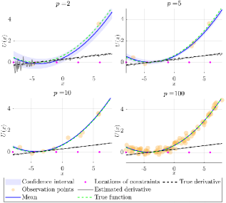
Notice that the error 𝐞tsuperscript𝐞𝑡{\mathbf{e}}^{t} is not assumed to have zero mean, since the GP may introduce a bias in the estimated gradient. Assumption 7 presumes that the expected value of 𝐞t2superscriptnormsuperscript𝐞𝑡2\|{\mathbf{e}}^{t}\|^{2} is bounded; this is consistent with standard assumptions in the context of inexact gradient methods and stochastic gradient methods (see, e.g., [32, 33]). We also note that E¯tsuperscript¯𝐸𝑡\bar{E}^{t} can be taken to be the Bayes errors for regression with GPs; in fact, [10] showed that the error of the GP regression is higher than the error incurred by the shape-constrained GP regression. We point out that Assumption 7 is also supported by empirical evidences; an example for the shape-constrained GP is provided in Figure 3, which illustrates the estimated function and the estimated derivative for different numbers of noisy functional evaluations. With these standard assumptions in place, the next section will provide performance bounds for the proposed algorithm.

IV-A Dynamic Regret

We characterize the performance of Algorithm 1 using the so-called dynamic regret (see, e.g., [21, 22, 17, 18] and references therein). In particular, given the distributed nature of our algorithm, we consider an extension of the network regret [17, 18] to a time-varying setting. To this end, define the dynamic regret per user j𝒩m𝑗subscript𝒩𝑚j\in\mathcal{N}_{m} interacting with the system m𝑚m, with respect to an optimal solution of (3) for the system m𝑚m at time t𝑡t, i.e., xmtsuperscriptsubscript𝑥𝑚𝑡x_{m}^{t*}, as

RegTm,j:=t=1Ti=1NmUm,i(xm,jt)t=1Ti=1NmUm,i(xmt).assignsuperscriptsubscriptReg𝑇𝑚𝑗superscriptsubscript𝑡1𝑇superscriptsubscript𝑖1subscript𝑁𝑚subscript𝑈𝑚𝑖superscriptsubscript𝑥𝑚𝑗𝑡superscriptsubscript𝑡1𝑇superscriptsubscript𝑖1subscript𝑁𝑚subscript𝑈𝑚𝑖superscriptsubscript𝑥𝑚𝑡\mathrm{Reg}_{T}^{m,j}:=\sum_{t=1}^{T}\sum_{i=1}^{N_{m}}{U}_{m,i}(x_{m,j}^{t})-\sum_{t=1}^{T}\sum_{i=1}^{N_{m}}{U}_{m,i}(x_{m}^{t*}). (11)

Then, based on (11), we define the dynamic network regret for the system m𝑚m as [17, 18]

RegTm=1Nmj=1NmRegTm,jsuperscriptsubscriptReg𝑇𝑚1subscript𝑁𝑚superscriptsubscript𝑗1subscript𝑁𝑚superscriptsubscriptReg𝑇𝑚𝑗\displaystyle\mathrm{Reg}_{T}^{m}=\frac{1}{N_{m}}\sum_{j=1}^{N_{m}}\mathrm{Reg}_{T}^{m,j}
=1Nmt=1Ti,j=1NmUm,i(xm,jt)t=1Ti=1NmUm,i(xmt).absent1subscript𝑁𝑚superscriptsubscript𝑡1𝑇superscriptsubscript𝑖𝑗1subscript𝑁𝑚subscript𝑈𝑚𝑖superscriptsubscript𝑥𝑚𝑗𝑡superscriptsubscript𝑡1𝑇superscriptsubscript𝑖1subscript𝑁𝑚subscript𝑈𝑚𝑖superscriptsubscript𝑥𝑚𝑡\displaystyle~{}~{}~{}~{}=\frac{1}{N_{m}}\sum_{t=1}^{T}\sum_{i,j=1}^{N_{m}}{U}_{m,i}(x_{m,j}^{t})-\sum_{t=1}^{T}\sum_{i=1}^{N_{m}}{U}_{m,i}(x_{m}^{t*}). (12)

By using (IV-A), the dynamic global network regret after T𝑇T iterations can be defined as

RegTsubscriptReg𝑇\displaystyle\mathrm{Reg}_{T} :=m=1MRegTm.assignabsentsuperscriptsubscript𝑚1𝑀superscriptsubscriptReg𝑇𝑚\displaystyle:=\sum_{m=1}^{M}\mathrm{Reg}_{T}^{m}. (13)

To analyze the global network regret, let 𝐱tsuperscript𝐱𝑡{\mathbf{x}}^{t*} be an optimal solution of (3) at time t𝑡t, and consider the following standard definitions of the path length, which captures the drift of the optimal solutions over T𝑇T time steps

ΦT:=t=1T𝐱t𝐱t+1,ΥT:=t=1T𝐱t𝐱t+12.formulae-sequenceassignsuperscriptΦ𝑇superscriptsubscript𝑡1𝑇normsuperscript𝐱𝑡superscript𝐱𝑡1assignsuperscriptΥ𝑇superscriptsubscript𝑡1𝑇superscriptnormsuperscript𝐱𝑡superscript𝐱𝑡12\displaystyle\Phi^{T}:=\sum_{t=1}^{T}\|{\mathbf{x}}^{t*}-{\mathbf{x}}^{t+1*}\|,\,\,\Upsilon^{T}:=\sum_{t=1}^{T}\|{\mathbf{x}}^{t*}-{\mathbf{x}}^{t+1*}\|^{2}. (14)

Further, consider the following definitions for the cumulative expected error in the gradient:

ξT:=t=1T𝔼[𝐞t|t],ΞT:=t=1TE¯t.formulae-sequenceassignsuperscript𝜉𝑇superscriptsubscript𝑡1𝑇𝔼delimited-[]conditionalnormsuperscript𝐞𝑡subscript𝑡assignsuperscriptΞ𝑇superscriptsubscript𝑡1𝑇superscript¯𝐸𝑡\displaystyle\xi^{T}:=\sum_{t=1}^{T}{\mathbb{E}}[\|{\mathbf{e}}^{t}\||\mathcal{F}_{t}],\qquad\Xi^{T}:=\sum_{t=1}^{T}\bar{E}^{t}. (15)

With these metrics in place, we start by bounding the norm of the true gradient of the time-varying Lagrangian with respect to the primal variable for any 𝐱𝒳t𝐱superscript𝒳𝑡{\mathbf{x}}\in{\mathcal{X}}^{t}, νΨt𝜈superscriptΨ𝑡\nu\in\Psi^{t} and 𝝀Λt𝝀superscriptΛ𝑡{\mbox{\boldmath$\lambda$}}\in\Lambda^{t}. Let J:=supt𝒯max𝐱𝒳tCt(𝐲t(𝐱))assign𝐽𝑡𝒯supremum𝐱superscript𝒳𝑡normsuperscript𝐶𝑡superscript𝐲𝑡𝐱J:=\underset{t\in{\mathcal{T}}}{\sup}\,\underset{{\mathbf{x}}\in{\mathcal{X}}^{t}}{\max}\|\nabla C^{t}({\mathbf{y}}^{t}({\mathbf{x}}))\| by Assumption 1 and Assumption 2, Bλ:=supt𝒯maxλΛt𝝀assignsubscript𝐵𝜆𝑡𝒯supremum𝜆superscriptΛ𝑡norm𝝀B_{\lambda}:=\underset{t\in{\mathcal{T}}}{\sup}\,\underset{\lambda\in\Lambda^{t}}{\max}\|{\mbox{\boldmath$\lambda$}}\| and Bν:=supt𝒯maxνΨt|ν|assignsubscript𝐵𝜈𝑡𝒯supremum𝜈superscriptΨ𝑡𝜈B_{\nu}:=\underset{t\in{\mathcal{T}}}{\sup}\,\underset{\nu\in\Psi^{t}}{\max}\,|\nu| under Assumption 5 and Assumption 6, then we have

𝐱t(𝐱,ν,𝝀)normsubscript𝐱superscript𝑡𝐱𝜈𝝀\displaystyle\|\nabla_{{\mathbf{x}}}{\mathcal{L}}^{t}({\mathbf{x}},\nu,{\mbox{\boldmath$\lambda$}})\| f(𝐱)+νCt(𝐲t(𝐱))+𝐃𝝀absentnorm𝑓𝐱𝜈normsuperscript𝐶𝑡superscript𝐲𝑡𝐱normsuperscript𝐃top𝝀\displaystyle\leq\|\nabla f({\mathbf{x}})\|+\nu\|\nabla C^{t}({\mathbf{y}}^{t}({\mathbf{x}}))\|+\|{\mathbf{D}}^{\top}{\mbox{\boldmath$\lambda$}}\|
L+BνJ+ΩBλ:=Γx,absent𝐿subscript𝐵𝜈𝐽Ωsubscript𝐵𝜆assignsubscriptΓ𝑥\displaystyle\leq L+B_{\nu}J+\Omega B_{\lambda}:=\Gamma_{x}, (16)

where, the last inequality holds by using the triangle and Cauchy-Schwarz inequality, and Assumption 3. The term Γx=L+BνJ+ΩBλsubscriptΓ𝑥𝐿subscript𝐵𝜈𝐽Ωsubscript𝐵𝜆\Gamma_{x}=L+B_{\nu}J+\Omega B_{\lambda} is an upper bound for the gradient of the Lagrangian with respect to 𝐱𝐱{\mathbf{x}}.

Similarly, we bound the norm of the gradient of the Lagrangian with respect to the dual variables 𝝀𝝀\lambda and ν𝜈\nu for any 𝐱𝒳t𝐱superscript𝒳𝑡{\mathbf{x}}\in{\mathcal{X}}^{t}, νΨt𝜈superscriptΨ𝑡\nu\in\Psi^{t} and 𝝀Λt𝝀superscriptΛ𝑡{\mbox{\boldmath$\lambda$}}\in\Lambda^{t}. Let 𝜿=[ν,𝝀]𝜿superscript𝜈superscript𝝀toptop{\mbox{\boldmath$\kappa$}}=[\nu,{\mbox{\boldmath$\lambda$}}^{\top}]^{\top}, |Ct(𝐲t(𝐱))|H<superscript𝐶𝑡superscript𝐲𝑡𝐱𝐻\left|C^{t}({\mathbf{y}}^{t}({\mathbf{x}}))\right|\leq H<\infty for all t𝑡t by Assumption 1 and Assumption 2, and Bx:=supt𝒯max𝐱𝒳t𝐱assignsubscript𝐵𝑥𝑡𝒯supremum𝐱superscript𝒳𝑡norm𝐱B_{x}:=\underset{t\in{\mathcal{T}}}{\sup}\,\underset{{\mathbf{x}}\in{\mathcal{X}}^{t}}{\max}\|{\mathbf{x}}\| under Assumption 1. Then, κt(𝐱,𝜿)2superscriptnormsubscript𝜅superscript𝑡𝐱𝜿2\|\nabla_{\kappa}{\mathcal{L}}^{t}({\mathbf{x}},{\mbox{\boldmath$\kappa$}})\|^{2} can be bounded by

κt(𝐱,𝜿)2superscriptnormsubscript𝜅superscript𝑡𝐱𝜿2\displaystyle\|\nabla_{\kappa}{\mathcal{L}}^{t}({\mathbf{x}},{\mbox{\boldmath$\kappa$}})\|^{2} =λt(𝐱,ν,𝝀)νt(𝐱,ν,𝝀)2,absentsuperscriptnormmatrixsubscript𝜆superscript𝑡𝐱𝜈𝝀subscript𝜈superscript𝑡𝐱𝜈𝝀2\displaystyle=\left\|\begin{matrix}\nabla_{\lambda}{\mathcal{L}}^{t}({\mathbf{x}},\nu,{\mbox{\boldmath$\lambda$}})\\ \nabla_{\nu}{\mathcal{L}}^{t}({\mathbf{x}},\nu,{\mbox{\boldmath$\lambda$}})\end{matrix}\right\|^{2},
Ω2Bx2+H2:=Γκ,absentsuperscriptΩ2superscriptsubscript𝐵𝑥2superscript𝐻2assignsubscriptΓ𝜅\displaystyle\leq\Omega^{2}B_{x}^{2}+H^{2}:=\Gamma_{\kappa}, (17)

where we used the Cauchy-Schwarz inequality, Assumption 1, and Assumption 3. Further, let diam(𝒳t)Dxtdiamsuperscript𝒳𝑡subscriptsuperscript𝐷𝑡𝑥\mathrm{diam}({\mathcal{X}}^{t})\leq D^{t}_{x} where DxtDx<subscriptsuperscript𝐷𝑡𝑥subscript𝐷𝑥D^{t}_{x}\leq D_{x}<\infty by Assumption 1. The term Γκ=Ω2Bx2+H2subscriptΓ𝜅superscriptΩ2superscriptsubscript𝐵𝑥2superscript𝐻2\Gamma_{\kappa}=\Omega^{2}B_{x}^{2}+H^{2} is an upper bound for the gradient of the Lagrangian with respect to 𝜿𝜿\kappa.

With these notations in place, we are now ready to state the main result for the dynamic regret.

Theorem 1

Let Assumptions 1-7 hold. Set 𝛌1=𝟎superscript𝛌10{\mbox{\boldmath$\lambda$}}^{1}=\mathbf{0}, ν1=0superscript𝜈10\nu^{1}=0. Then, the dynamic network regret after T𝑇T iterations is upper bounded by

𝔼[RegT]12α(𝐱1𝐱12+Bλ2+Bν2)+α2T(Γx2+Γκ)𝔼delimited-[]subscriptReg𝑇12𝛼superscriptnormsuperscript𝐱1superscript𝐱12superscriptsubscript𝐵𝜆2superscriptsubscript𝐵𝜈2𝛼2𝑇superscriptsubscriptΓ𝑥2subscriptΓ𝜅\displaystyle{\mathbb{E}}[\mathrm{Reg}_{T}]\leq\frac{1}{2\alpha}(\|{\mathbf{x}}^{1}-{\mathbf{x}}^{1*}\|^{2}+B_{\lambda}^{2}+B_{\nu}^{2})+\frac{\alpha}{2}T(\Gamma_{x}^{2}+\Gamma_{\kappa})
+α2ΞT+ξT(2Bx+αΓx)+12αΥT+1αDxΦT.𝛼2superscriptΞ𝑇superscript𝜉𝑇2subscript𝐵𝑥𝛼subscriptΓ𝑥12𝛼superscriptΥ𝑇1𝛼subscript𝐷𝑥superscriptΦ𝑇\displaystyle\quad+\frac{\alpha}{2}\Xi^{T}+\xi^{T}\,(2B_{x}+\alpha\Gamma_{x})+\frac{1}{2\alpha}\Upsilon^{T}+\frac{1}{\alpha}D_{x}\Phi^{T}. (18)

The proof of this theorem will be provided in Section IV-C. Theorem 1 asserts that the bound on the expected dynamic network regret 𝔼[RegT]𝔼delimited-[]subscriptReg𝑇{\mathbb{E}}[\mathrm{Reg}_{T}] after T𝑇T time steps depends on the temporal variability of the solutions (through the terms 12αΥT12𝛼superscriptΥ𝑇\frac{1}{2\alpha}\Upsilon^{T} and 1αDxΦT1𝛼subscript𝐷𝑥superscriptΦ𝑇\frac{1}{\alpha}D_{x}\Phi^{T}) and the errors associated with the estimation of the gradient (through the terms α2ΞT𝛼2superscriptΞ𝑇\frac{\alpha}{2}\Xi^{T} and ξT(2Bx+αΓx)superscript𝜉𝑇2subscript𝐵𝑥𝛼subscriptΓ𝑥\xi^{T}(2B_{x}+\alpha\Gamma_{x})). The remaining terms are in line with standard regret results (e.g., [17]). In particular, we can observe the following:

\bullet Persistent variations and gradient errors: Suppose that ΥTsuperscriptΥ𝑇\Upsilon^{T} and ΦTsuperscriptΦ𝑇\Phi^{T} grow as 𝒪(T)𝒪𝑇\mathcal{O}(T), modeling a persistent temporal variation of the constraints and/or the vector 𝐰tsuperscript𝐰𝑡{\mathbf{w}}^{t}; suppose further that ΞTsuperscriptΞ𝑇\Xi^{T} and ξTsuperscript𝜉𝑇\xi^{T} grow as 𝒪(T)𝒪𝑇\mathcal{O}(T), modeling a persistent error in the gradient 𝐠tsuperscript𝐠𝑡{\mathbf{g}}^{t}. Then, 𝔼[RegT]/T𝔼delimited-[]subscriptReg𝑇𝑇{\mathbb{E}}[\mathrm{Reg}_{T}]/T behaves as 𝒪(1)𝒪1\mathcal{O}(1).

\bullet Vanishing gradient errors: If ΞTsuperscriptΞ𝑇\Xi^{T} and ξTsuperscript𝜉𝑇\xi^{T} grows sublinearly, i.e., as o(T)𝑜𝑇o(T), then the asymptotic average regret is in general 1T𝔼[RegT]=𝒪(1+T1ΥT+T1ΦT)1𝑇𝔼delimited-[]subscriptReg𝑇𝒪1superscript𝑇1superscriptΥ𝑇superscript𝑇1superscriptΦ𝑇\frac{1}{T}{\mathbb{E}}[\mathrm{Reg}_{T}]=\mathcal{O}(1+T^{-1}\Upsilon^{T}+T^{-1}\Phi^{T}). Notice that if the algorithm is executed over a finite interval of T𝑇T steps and the step-size is chosen as α=1T𝛼1𝑇\alpha=\frac{1}{\sqrt{T}}, then 𝔼[RegT]/T𝔼delimited-[]subscriptReg𝑇𝑇{\mathbb{E}}[\mathrm{Reg}_{T}]/T behaves as 1T𝔼[RegT]=𝒪(T12+T12ΥT+T12ΦT)1𝑇𝔼delimited-[]subscriptReg𝑇𝒪superscript𝑇12superscript𝑇12superscriptΥ𝑇superscript𝑇12superscriptΦ𝑇\frac{1}{T}{\mathbb{E}}[\mathrm{Reg}_{T}]=\mathcal{O}(T^{-\frac{1}{2}}+T^{-\frac{1}{2}}\Upsilon^{T}+T^{-\frac{1}{2}}\Phi^{T})   .

\bullet Vanishing variations and errors: If ΥTsuperscriptΥ𝑇\Upsilon^{T}, ΦTsuperscriptΦ𝑇\Phi^{T}, ΞTsuperscriptΞ𝑇\Xi^{T}, and ξTsuperscript𝜉𝑇\xi^{T} all grow as o(T)𝑜𝑇o(T), then we recover the asymptotic result of [17].

Remark 3

Regarding the errors in the gradient, if the function Um,nsubscript𝑈𝑚𝑛U_{m,n} is strongly convex, then the estimation error yielded by a shape-constrained GPs will decrease with the increasing of the number of functional evaluations; see the illustrative example in Figure 3, and the discussion in [10]. However, zeroth-order and finite-different methods will still generate an error in the estimation of the gradient, and thus ΞTsuperscriptΞ𝑇\Xi^{T} and ξTsuperscript𝜉𝑇\xi^{T} would generally increase as 𝒪(T)𝒪𝑇{\mathcal{O}}(T). To obtain a trend as o(T)𝑜𝑇o(T), one has to increase the accuracy in the gradient estimation to make 𝐞tsuperscript𝐞𝑡{\mathbf{e}}^{t} arbitrarily small. \Box

IV-B Average Constraint Violation

We now consider a bound on the violation of the constraint on the network output 𝐲tsuperscript𝐲𝑡{\mathbf{y}}^{t}. To this end, we consider the so-called average constraint violation (ACV), which we define here as

ACVT:=t=1T[Ct(𝐲t(𝐱t))]+.assignsubscriptACV𝑇superscriptsubscript𝑡1𝑇superscriptdelimited-[]superscript𝐶𝑡superscript𝐲𝑡superscript𝐱𝑡\displaystyle\mathrm{ACV}_{T}:=\sum_{t=1}^{T}\left[C^{t}({\mathbf{y}}^{t}({\mathbf{x}}^{t}))\right]^{+}. (19)

We note that some prior works in context (e.g., [19, 34]) consider the modified definition [t=1TCt(𝐲t(𝐱t))]+superscriptdelimited-[]superscriptsubscript𝑡1𝑇superscript𝐶𝑡superscript𝐲𝑡superscript𝐱𝑡\left[\sum_{t=1}^{T}C^{t}({\mathbf{y}}^{t}({\mathbf{x}}^{t}))\right]^{+}, which may lead to looser bounds.

Theorem 2

Let Assumptions 1-7 hold. Then, the average constraint violation incurred by the algorithm (5) can be bounded as

𝔼[ACVT]Bν1T(DxL+BλΩBx)𝔼delimited-[]subscriptACV𝑇superscriptsubscript𝐵𝜈1𝑇subscript𝐷𝑥𝐿subscript𝐵𝜆Ωsubscript𝐵𝑥\displaystyle{\mathbb{E}}\left[\mathrm{ACV}_{T}\right]\leq B_{\nu}^{-1}T\left(D_{x}L+B_{\lambda}\Omega B_{x}\right)
+Bν1(α2ΞT+ξT(2Bx+αΓx)+12αΥT+1αDxΦT)superscriptsubscript𝐵𝜈1𝛼2superscriptΞ𝑇superscript𝜉𝑇2subscript𝐵𝑥𝛼subscriptΓ𝑥12𝛼superscriptΥ𝑇1𝛼subscript𝐷𝑥superscriptΦ𝑇\displaystyle~{}~{}~{}+B_{\nu}^{-1}\left(\frac{\alpha}{2}\Xi^{T}+\xi^{T}(2B_{x}+\alpha\Gamma_{x})+\frac{1}{2\alpha}\Upsilon^{T}+\frac{1}{\alpha}D_{x}\Phi^{T}\right)
+Bν1T(1α(4Bx2+Bν2)+α2(Γx2+H2)).superscriptsubscript𝐵𝜈1𝑇1𝛼4superscriptsubscript𝐵𝑥2superscriptsubscript𝐵𝜈2𝛼2superscriptsubscriptΓ𝑥2superscript𝐻2\displaystyle~{}~{}~{}+B_{\nu}^{-1}T\left(\frac{1}{\alpha}(4B_{x}^{2}+B_{\nu}^{2})+\frac{\alpha}{2}(\Gamma_{x}^{2}+H^{2})\right). (20)

The second and third terms of (20) exhibit the same asymptotic behavior of the dynamic regret under persistent variations and gradient errors, and with vanishing variations and errors. In case of vanishing variations and gradient errors, the bottlenecks are the two terms TDxL𝑇subscript𝐷𝑥𝐿TD_{x}L and TBλΩBx𝑇subscript𝐵𝜆Ωsubscript𝐵𝑥TB_{\lambda}\Omega B_{x}, which make 𝔼[ACVT]/T𝔼delimited-[]subscriptACV𝑇𝑇{\mathbb{E}}[\mathrm{ACV}_{T}]/T behave as 𝒪(1)𝒪1\mathcal{O}(1).

Refer to caption
Figure 3: Example of the derivative estimation using shape-constrained GPs with hyperparameters σf=1subscript𝜎𝑓1\sigma_{f}=1 and =1010\ell=10. As expected, the estimated derivative error decreases with the increasing of the number of observations p𝑝p. In this case, shape-constrained GP outperforms GP for low numbers of samples (see also Section V).

IV-C Proofs of the Results

To streamline exposition, define ϕt:=𝐱t𝐱t+1assignsuperscriptitalic-ϕ𝑡normsuperscript𝐱𝑡superscript𝐱𝑡1\phi^{t}:=\|{\mathbf{x}}^{t*}-{\mathbf{x}}^{t+1*}\| and e¯t:=𝔼[𝐞t|t]assignsuperscript¯e𝑡𝔼delimited-[]conditionalnormsuperscript𝐞𝑡subscript𝑡\bar{\mathrm{e}}^{t}:={\mathbb{E}}[\|{\mathbf{e}}^{t}\||\mathcal{F}_{t}]. To derive our main results, we will utilize the following lemma.

Lemma 1

Let Assumptions 1-7 hold, and set 𝛌1=𝟎superscript𝛌10{\mbox{\boldmath$\lambda$}}^{1}=\mathbf{0}, ν1=0superscript𝜈10\nu^{1}=0. Then, for any 𝛋Ψt×Λt𝛋superscriptΨ𝑡superscriptΛ𝑡{\mbox{\boldmath$\kappa$}}\in\Psi^{t}\times\Lambda^{t} the following holds:

𝔼[t=1T(t(𝐱t,𝜿)t(𝐱t,𝜿t))]𝔼delimited-[]superscriptsubscript𝑡1𝑇superscript𝑡superscript𝐱𝑡𝜿superscript𝑡superscript𝐱𝑡superscript𝜿𝑡\displaystyle{\mathbb{E}}\left[\sum_{t=1}^{T}\left({\mathcal{L}}^{t}({\mathbf{x}}^{t},{\mbox{\boldmath$\kappa$}})-{\mathcal{L}}^{t}({\mathbf{x}}^{t*},{\mbox{\boldmath$\kappa$}}^{t})\right)\right]
12α(𝐱1𝐱12+𝜿2)+α2T(Γx2+Γκ)absent12𝛼superscriptnormsuperscript𝐱1superscript𝐱12superscriptnorm𝜿2𝛼2𝑇superscriptsubscriptΓ𝑥2subscriptΓ𝜅\displaystyle\quad\leq\frac{1}{2\alpha}(\|{\mathbf{x}}^{1}-{\mathbf{x}}^{1*}\|^{2}+\|{\mbox{\boldmath$\kappa$}}\|^{2})+\frac{\alpha}{2}T(\Gamma_{x}^{2}+\Gamma_{\kappa})
+α2ΞT+ξT(2Bx+αΓx)+12αΥT+1αDxΦT.𝛼2superscriptΞ𝑇superscript𝜉𝑇2subscript𝐵𝑥𝛼subscriptΓ𝑥12𝛼superscriptΥ𝑇1𝛼subscript𝐷𝑥superscriptΦ𝑇\displaystyle\quad+\frac{\alpha}{2}\Xi^{T}+\xi^{T}\,(2B_{x}+\alpha\Gamma_{x})+\frac{1}{2\alpha}\Upsilon^{T}+\frac{1}{\alpha}D_{x}\Phi^{T}. (21)

Proof. Notice first that

~𝐱t(𝐱t,ν,𝝀)𝐱t(𝐱t,ν,𝝀)normsubscript~𝐱superscript𝑡superscript𝐱𝑡𝜈𝝀subscript𝐱superscript𝑡superscript𝐱𝑡𝜈𝝀\displaystyle\|\tilde{\nabla}_{{\mathbf{x}}}{\mathcal{L}}^{t}({\mathbf{x}}^{t},\nu,{\mbox{\boldmath$\lambda$}})-\nabla_{{\mathbf{x}}}{\mathcal{L}}^{t}({\mathbf{x}}^{t},\nu,{\mbox{\boldmath$\lambda$}})\| =𝐞t,absentnormsuperscript𝐞𝑡\displaystyle=\|{\mathbf{e}}^{t}\|, (22)

where ~𝐱t(𝐱t,ν,𝝀)subscript~𝐱superscript𝑡superscript𝐱𝑡𝜈𝝀\tilde{\nabla}_{{\mathbf{x}}}{\mathcal{L}}^{t}({\mathbf{x}}^{t},\nu,{\mbox{\boldmath$\lambda$}}) is the inexact gradient of the Lagrangian function (where we utilize 𝐠tsuperscript𝐠𝑡{\mathbf{g}}^{t} instead of f(𝐱t)𝑓superscript𝐱𝑡\nabla f({\mathbf{x}}^{t})). Recall that 𝐱tsuperscript𝐱𝑡{\mathbf{x}}^{t*} denotes an optimal solution at time t𝑡t. Using the primal update, adding and subtracting 𝐱tsuperscript𝐱𝑡{\mathbf{x}}^{t*}, we get:

𝐱t+1𝐱t+12=𝐱t+1𝐱t+𝐱t𝐱t+12superscriptnormsuperscript𝐱𝑡1superscript𝐱𝑡12superscriptnormsuperscript𝐱𝑡1superscript𝐱𝑡superscript𝐱𝑡superscript𝐱𝑡12\displaystyle\|{\mathbf{x}}^{t+1}-{\mathbf{x}}^{t+1*}\|^{2}=\|{\mathbf{x}}^{t+1}-{\mathbf{x}}^{t*}+{\mathbf{x}}^{t*}-{\mathbf{x}}^{t+1*}\|^{2}
=𝐱t+1𝐱t2+2(𝐱t+1𝐱t)(𝐱t𝐱t+1)absentsuperscriptnormsuperscript𝐱𝑡1superscript𝐱𝑡22superscriptsuperscript𝐱𝑡1superscript𝐱𝑡topsuperscript𝐱𝑡superscript𝐱𝑡1\displaystyle~{}~{}=\|{\mathbf{x}}^{t+1}-{\mathbf{x}}^{t*}\|^{2}+2({\mathbf{x}}^{t+1}-{\mathbf{x}}^{t*})^{\top}({\mathbf{x}}^{t*}-{\mathbf{x}}^{t+1*})
+𝐱t𝐱t+12,superscriptnormsuperscript𝐱𝑡superscript𝐱𝑡12\displaystyle~{}~{}\quad+\|{\mathbf{x}}^{t*}-{\mathbf{x}}^{t+1*}\|^{2},
=proj𝒳t{𝐱tα~𝐱t(𝐱t,νt,𝝀t)}𝐱t2+(ϕt)2absentsuperscriptnormsubscriptprojsuperscript𝒳𝑡superscript𝐱𝑡𝛼subscript~𝐱superscript𝑡superscript𝐱𝑡superscript𝜈𝑡superscript𝝀𝑡superscript𝐱𝑡2superscriptsuperscriptitalic-ϕ𝑡2\displaystyle~{}~{}=\left\|\mathrm{proj}_{{{\mathcal{X}}^{t}}}\left\{{\mathbf{x}}^{t}-\alpha\tilde{\nabla}_{{\mathbf{x}}}{\mathcal{L}}^{t}({\mathbf{x}}^{t},\nu^{t},{\mbox{\boldmath$\lambda$}}^{t})\right\}-{\mathbf{x}}^{t*}\right\|^{2}+(\phi^{t})^{2}
+2(𝐱t+1𝐱(,t))(𝐱t𝐱t+1),2superscriptsuperscript𝐱𝑡1superscript𝐱𝑡topsuperscript𝐱𝑡superscript𝐱𝑡1\displaystyle~{}~{}\quad+2({\mathbf{x}}^{t+1}-{\mathbf{x}}^{(*,t)})^{\top}({\mathbf{x}}^{t*}-{\mathbf{x}}^{t+1*}),
𝐱tα~𝐱t(𝐱t,νt,𝝀t)𝐱t2+(ϕt)2absentsuperscriptnormsuperscript𝐱𝑡𝛼subscript~𝐱superscript𝑡superscript𝐱𝑡superscript𝜈𝑡superscript𝝀𝑡superscript𝐱𝑡2superscriptsuperscriptitalic-ϕ𝑡2\displaystyle~{}~{}\leq\|{\mathbf{x}}^{t}-\alpha\tilde{\nabla}_{{\mathbf{x}}}{\mathcal{L}}^{t}({\mathbf{x}}^{t},\nu^{t},{\mbox{\boldmath$\lambda$}}^{t})-{\mathbf{x}}^{t*}\|^{2}+(\phi^{t})^{2}
+2𝐱t+1𝐱t𝐱t𝐱t+1,2normsuperscript𝐱𝑡1superscript𝐱𝑡normsuperscript𝐱𝑡superscript𝐱𝑡1\displaystyle~{}~{}\quad+2\|{\mathbf{x}}^{t+1}-{\mathbf{x}}^{t*}\|\|{\mathbf{x}}^{t*}-{\mathbf{x}}^{t+1*}\|,
𝐱t𝐱tα~𝐱t(𝐱t,νt,𝝀t)2+(ϕt)2+2Dxϕt,absentsuperscriptnormsuperscript𝐱𝑡superscript𝐱𝑡𝛼subscript~𝐱superscript𝑡superscript𝐱𝑡superscript𝜈𝑡superscript𝝀𝑡2superscriptsuperscriptitalic-ϕ𝑡22subscript𝐷𝑥superscriptitalic-ϕ𝑡\displaystyle~{}~{}\leq\|{\mathbf{x}}^{t}-{\mathbf{x}}^{t*}-\alpha\tilde{\nabla}_{{\mathbf{x}}}{\mathcal{L}}^{t}({\mathbf{x}}^{t},\nu^{t},{\mbox{\boldmath$\lambda$}}^{t})\|^{2}+(\phi^{t})^{2}+2D_{x}\phi^{t}, (23)

where (23) holds by the non-expansiveness property of the projection operator, the Cauchy-Schwarz inequality, and the definition of ϕtsuperscriptitalic-ϕ𝑡\phi^{t}.

By adding and subtracting α𝐱t(𝐱t,νt,𝝀t)𝛼subscript𝐱superscript𝑡superscript𝐱𝑡superscript𝜈𝑡superscript𝝀𝑡\alpha\nabla_{\mathbf{x}}{\mathcal{L}}^{t}({\mathbf{x}}^{t},\nu^{t},{\mbox{\boldmath$\lambda$}}^{t}) (to simplify notation we use 𝐱t=𝐱t(𝐱t,νt,𝝀t)subscript𝐱superscript𝑡subscript𝐱superscript𝑡superscript𝐱𝑡superscript𝜈𝑡superscript𝝀𝑡\nabla_{\mathbf{x}}{\mathcal{L}}^{t}=\nabla_{\mathbf{x}}{\mathcal{L}}^{t}({\mathbf{x}}^{t},\nu^{t},{\mbox{\boldmath$\lambda$}}^{t})), and expanding the first term of the right-hand side (RHS) of (23), we get

𝐱t𝐱tα~𝐱t2superscriptnormsuperscript𝐱𝑡superscript𝐱𝑡𝛼subscript~𝐱superscript𝑡2\displaystyle\|{\mathbf{x}}^{t}-{\mathbf{x}}^{t*}-\alpha\tilde{\nabla}_{{\mathbf{x}}}{\mathcal{L}}^{t}\|^{2}
=𝐱t𝐱tα𝐱t+α(𝐱t~𝐱t)2,absentsuperscriptnormsuperscript𝐱𝑡superscript𝐱𝑡𝛼subscript𝐱superscript𝑡𝛼subscript𝐱superscript𝑡subscript~𝐱superscript𝑡2\displaystyle\quad=\|{\mathbf{x}}^{t}-{\mathbf{x}}^{t*}-\alpha\nabla_{{\mathbf{x}}}{\mathcal{L}}^{t}+\alpha(\nabla_{{\mathbf{x}}}{\mathcal{L}}^{t}-\tilde{\nabla}_{{\mathbf{x}}}{\mathcal{L}}^{t})\|^{2},
=𝐱t𝐱tα𝐱t2+α2𝐱t~𝐱t2absentsuperscriptnormsuperscript𝐱𝑡superscript𝐱𝑡𝛼subscript𝐱superscript𝑡2superscript𝛼2superscriptnormsubscript𝐱superscript𝑡subscript~𝐱superscript𝑡2\displaystyle\quad=\|{\mathbf{x}}^{t}-{\mathbf{x}}^{t*}-\alpha\nabla_{{\mathbf{x}}}{\mathcal{L}}^{t}\|^{2}+\alpha^{2}\|\nabla_{{\mathbf{x}}}{\mathcal{L}}^{t}-\tilde{\nabla}_{{\mathbf{x}}}{\mathcal{L}}^{t}\|^{2}
+2α(𝐱t𝐱tα𝐱t)(𝐱t~𝐱t),2𝛼superscriptsuperscript𝐱𝑡superscript𝐱𝑡𝛼subscript𝐱superscript𝑡topsubscript𝐱superscript𝑡subscript~𝐱superscript𝑡\displaystyle\quad\quad+2\alpha({\mathbf{x}}^{t}-{\mathbf{x}}^{t*}-\alpha\nabla_{{\mathbf{x}}}{\mathcal{L}}^{t})^{\top}(\nabla_{{\mathbf{x}}}{\mathcal{L}}^{t}-\tilde{\nabla}_{{\mathbf{x}}}{\mathcal{L}}^{t}),
𝐱t𝐱tα𝐱t2+α2𝐱t~𝐱t2absentsuperscriptnormsuperscript𝐱𝑡superscript𝐱𝑡𝛼subscript𝐱superscript𝑡2superscript𝛼2superscriptnormsubscript𝐱superscript𝑡subscript~𝐱superscript𝑡2\displaystyle\quad\leq\|{\mathbf{x}}^{t}-{\mathbf{x}}^{t*}-\alpha\nabla_{{\mathbf{x}}}{\mathcal{L}}^{t}\|^{2}+\alpha^{2}\|\nabla_{{\mathbf{x}}}{\mathcal{L}}^{t}-\tilde{\nabla}_{{\mathbf{x}}}{\mathcal{L}}^{t}\|^{2}
+2α𝐱t𝐱tα𝐱t𝐱t~𝐱t.2𝛼normsuperscript𝐱𝑡superscript𝐱𝑡𝛼subscript𝐱superscript𝑡normsubscript𝐱superscript𝑡subscript~𝐱superscript𝑡\displaystyle\quad\quad+2\alpha\|{\mathbf{x}}^{t}-{\mathbf{x}}^{t*}-\alpha\nabla_{{\mathbf{x}}}{\mathcal{L}}^{t}\|\|\nabla_{{\mathbf{x}}}{\mathcal{L}}^{t}-\tilde{\nabla}_{{\mathbf{x}}}{\mathcal{L}}^{t}\|. (24)

By using (22), we have that (24) can be bounded as

𝐱t𝐱tα~𝐱t2superscriptnormsuperscript𝐱𝑡superscript𝐱𝑡𝛼subscript~𝐱superscript𝑡2\displaystyle\|{\mathbf{x}}^{t}-{\mathbf{x}}^{t*}-\alpha\tilde{\nabla}_{{\mathbf{x}}}{\mathcal{L}}^{t}\|^{2}
𝐱t𝐱tα𝐱t2+α2𝐞t2absentsuperscriptnormsuperscript𝐱𝑡superscript𝐱𝑡𝛼subscript𝐱superscript𝑡2superscript𝛼2superscriptnormsuperscript𝐞𝑡2\displaystyle\quad\leq\|{\mathbf{x}}^{t}-{\mathbf{x}}^{t*}-\alpha\nabla_{{\mathbf{x}}}{\mathcal{L}}^{t}\|^{2}+\alpha^{2}\|{\mathbf{e}}^{t}\|^{2}
+2α𝐞t𝐱t𝐱tα𝐱t,2𝛼normsuperscript𝐞𝑡normsuperscript𝐱𝑡superscript𝐱𝑡𝛼subscript𝐱superscript𝑡\displaystyle\quad\quad+2\alpha\|{\mathbf{e}}^{t}\|\,\|{\mathbf{x}}^{t}-{\mathbf{x}}^{t*}-\alpha\nabla_{{\mathbf{x}}}{\mathcal{L}}^{t}\|,
𝐱t𝐱tα𝐱t2+α2𝐞t2absentsuperscriptnormsuperscript𝐱𝑡superscript𝐱𝑡𝛼subscript𝐱superscript𝑡2superscript𝛼2superscriptnormsuperscript𝐞𝑡2\displaystyle\quad\leq\|{\mathbf{x}}^{t}-{\mathbf{x}}^{t*}-\alpha\nabla_{{\mathbf{x}}}{\mathcal{L}}^{t}\|^{2}+\alpha^{2}\|{\mathbf{e}}^{t}\|^{2}
+2α𝐞t(𝐱t𝐱t+α𝐱t),2𝛼normsuperscript𝐞𝑡normsuperscript𝐱𝑡superscript𝐱𝑡𝛼normsubscript𝐱superscript𝑡\displaystyle\quad\quad+2\alpha\|{\mathbf{e}}^{t}\|\,(\|{\mathbf{x}}^{t}-{\mathbf{x}}^{t*}\|+\alpha\|\nabla_{{\mathbf{x}}}{\mathcal{L}}^{t}\|),
𝐱t𝐱tα𝐱t2+α2𝐞t2+2α𝐞t(2Bx+αΓx),absentsuperscriptnormsuperscript𝐱𝑡superscript𝐱𝑡𝛼subscript𝐱superscript𝑡2superscript𝛼2superscriptnormsuperscript𝐞𝑡22𝛼normsuperscript𝐞𝑡2subscript𝐵𝑥𝛼subscriptΓ𝑥\displaystyle\quad\leq\|{\mathbf{x}}^{t}-{\mathbf{x}}^{t*}-\alpha\nabla_{{\mathbf{x}}}{\mathcal{L}}^{t}\|^{2}+\alpha^{2}\|{\mathbf{e}}^{t}\|^{2}+2\alpha\|{\mathbf{e}}^{t}\|\,(2B_{x}+\alpha\Gamma_{x}), (25)

where the last inequality is derived using (16) and the triangle inequality. By expanding the first term on the RHS of (25), we get

𝐱t𝐱tα𝐱t2superscriptnormsuperscript𝐱𝑡superscript𝐱𝑡𝛼subscript𝐱superscript𝑡2\displaystyle\|{\mathbf{x}}^{t}-{\mathbf{x}}^{t*}-\alpha\nabla_{{\mathbf{x}}}{\mathcal{L}}^{t}\|^{2}
=𝐱t𝐱t2+α2𝐱t22α(𝐱t𝐱t)𝐱t,absentsuperscriptnormsuperscript𝐱𝑡superscript𝐱𝑡2superscript𝛼2superscriptnormsubscript𝐱superscript𝑡22𝛼superscriptsuperscript𝐱𝑡superscript𝐱𝑡topsubscript𝐱superscript𝑡\displaystyle\quad=\|{\mathbf{x}}^{t}-{\mathbf{x}}^{t*}\|^{2}+\alpha^{2}\|\nabla_{{\mathbf{x}}}{\mathcal{L}}^{t}\|^{2}-2\alpha({\mathbf{x}}^{t}-{\mathbf{x}}^{t*})^{\top}\nabla_{{\mathbf{x}}}{\mathcal{L}}^{t},
𝐱t𝐱t2+α2Γx2absentsuperscriptnormsuperscript𝐱𝑡superscript𝐱𝑡2superscript𝛼2superscriptsubscriptΓ𝑥2\displaystyle\quad\leq\|{\mathbf{x}}^{t}-{\mathbf{x}}^{t*}\|^{2}+\alpha^{2}\Gamma_{x}^{2}
2α[t(𝐱t,νt,𝝀t)t(𝐱t,νt,𝝀t)].2𝛼delimited-[]superscript𝑡superscript𝐱𝑡superscript𝜈𝑡superscript𝝀𝑡superscript𝑡superscript𝐱𝑡superscript𝜈𝑡superscript𝝀𝑡\displaystyle\quad\quad-2\alpha[{\mathcal{L}}^{t}({\mathbf{x}}^{t},\nu^{t},{\mbox{\boldmath$\lambda$}}^{t})-{\mathcal{L}}^{t}({\mathbf{x}}^{t*},\nu^{t},{\mbox{\boldmath$\lambda$}}^{t})]. (26)

Since the function f(𝐱)𝑓𝐱f({\mathbf{x}}) is convex, the time-varying Lagrangian is convex in 𝐱𝐱{\mathbf{x}}. Thus, from the first-order characterization of convexity (26) holds.

Using (26) the bound (25), one has that

𝐱t𝐱tα~𝐱t2superscriptnormsuperscript𝐱𝑡superscript𝐱𝑡𝛼subscript~𝐱superscript𝑡2\displaystyle\|{\mathbf{x}}^{t}-{\mathbf{x}}^{t*}-\alpha\tilde{\nabla}_{{\mathbf{x}}}{\mathcal{L}}^{t}\|^{2}
𝐱t𝐱t2+α2Γx2+α2𝐞t2+2α𝐞t(2Bx+αΓx)absentsuperscriptnormsuperscript𝐱𝑡superscript𝐱𝑡2superscript𝛼2superscriptsubscriptΓ𝑥2superscript𝛼2superscriptnormsuperscript𝐞𝑡22𝛼normsuperscript𝐞𝑡2subscript𝐵𝑥𝛼subscriptΓ𝑥\displaystyle\quad\leq\|{\mathbf{x}}^{t}-{\mathbf{x}}^{t*}\|^{2}+\alpha^{2}\Gamma_{x}^{2}+\alpha^{2}\|{\mathbf{e}}^{t}\|^{2}+2\alpha\|{\mathbf{e}}^{t}\|\,(2B_{x}+\alpha\Gamma_{x})
2α[t(𝐱t,νt,𝝀t)t(𝐱t,νt,𝝀t)].2𝛼delimited-[]superscript𝑡superscript𝐱𝑡superscript𝜈𝑡superscript𝝀𝑡superscript𝑡superscript𝐱𝑡superscript𝜈𝑡superscript𝝀𝑡\displaystyle\quad\quad-2\alpha[{\mathcal{L}}^{t}({\mathbf{x}}^{t},\nu^{t},{\mbox{\boldmath$\lambda$}}^{t})-{\mathcal{L}}^{t}({\mathbf{x}}^{t*},\nu^{t},{\mbox{\boldmath$\lambda$}}^{t})]. (27)

By using (27) in (23), we have

𝐱t+1𝐱t+12superscriptnormsuperscript𝐱𝑡1superscript𝐱𝑡12\displaystyle\|{\mathbf{x}}^{t+1}-{\mathbf{x}}^{t+1*}\|^{2}
𝐱t𝐱t2+α2Γx2+α2𝐞t2+2α𝐞t(2Bx+αΓx)absentsuperscriptnormsuperscript𝐱𝑡superscript𝐱𝑡2superscript𝛼2superscriptsubscriptΓ𝑥2superscript𝛼2superscriptnormsuperscript𝐞𝑡22𝛼normsuperscript𝐞𝑡2subscript𝐵𝑥𝛼subscriptΓ𝑥\displaystyle\leq\|{\mathbf{x}}^{t}-{\mathbf{x}}^{t*}\|^{2}+\alpha^{2}\Gamma_{x}^{2}+\alpha^{2}\|{\mathbf{e}}^{t}\|^{2}+2\alpha\|{\mathbf{e}}^{t}\|\,(2B_{x}+\alpha\Gamma_{x})
2α[t(𝐱t,νt,𝝀t)t(𝐱t,νt,𝝀t)]+(ϕt)2+2Dxϕt.2𝛼delimited-[]superscript𝑡superscript𝐱𝑡superscript𝜈𝑡superscript𝝀𝑡superscript𝑡superscript𝐱𝑡superscript𝜈𝑡superscript𝝀𝑡superscriptsuperscriptitalic-ϕ𝑡22subscript𝐷𝑥superscriptitalic-ϕ𝑡\displaystyle-2\alpha[{\mathcal{L}}^{t}({\mathbf{x}}^{t},\nu^{t},{\mbox{\boldmath$\lambda$}}^{t})-{\mathcal{L}}^{t}({\mathbf{x}}^{t*},\nu^{t},{\mbox{\boldmath$\lambda$}}^{t})]+(\phi^{t})^{2}+2D_{x}\phi^{t}. (28)

It thus follows that:

t(𝐱t,νt,𝝀t)t(𝐱t,νt,𝝀t)superscript𝑡superscript𝐱𝑡superscript𝜈𝑡superscript𝝀𝑡superscript𝑡superscript𝐱𝑡superscript𝜈𝑡superscript𝝀𝑡\displaystyle{\mathcal{L}}^{t}({\mathbf{x}}^{t},\nu^{t},{\mbox{\boldmath$\lambda$}}^{t})-{\mathcal{L}}^{t}({\mathbf{x}}^{t*},\nu^{t},{\mbox{\boldmath$\lambda$}}^{t})
12α(𝐱t𝐱t2𝐱t+1𝐱t+12)+α2Γx2absent12𝛼superscriptnormsuperscript𝐱𝑡superscript𝐱𝑡2superscriptnormsuperscript𝐱𝑡1superscript𝐱𝑡12𝛼2superscriptsubscriptΓ𝑥2\displaystyle\leq\frac{1}{2\alpha}(\|{\mathbf{x}}^{t}-{\mathbf{x}}^{t*}\|^{2}-\|{\mathbf{x}}^{t+1}-{\mathbf{x}}^{t+1*}\|^{2})+\frac{\alpha}{2}\Gamma_{x}^{2}
+α2𝐞t2+𝐞t(2Bx+αΓx)+12α(ϕt)2+1αDxϕt.𝛼2superscriptnormsuperscript𝐞𝑡2normsuperscript𝐞𝑡2subscript𝐵𝑥𝛼subscriptΓ𝑥12𝛼superscriptsuperscriptitalic-ϕ𝑡21𝛼subscript𝐷𝑥superscriptitalic-ϕ𝑡\displaystyle+\frac{\alpha}{2}\|{\mathbf{e}}^{t}\|^{2}+\|{\mathbf{e}}^{t}\|\,(2B_{x}+\alpha\Gamma_{x})+\frac{1}{2\alpha}(\phi^{t})^{2}+\frac{1}{\alpha}D_{x}\phi^{t}. (29)

Now, we proceed with a similar analysis for the distance between the updates of the dual variables 𝝀t+1,νt+1superscript𝝀𝑡1superscript𝜈𝑡1{\mbox{\boldmath$\lambda$}}^{t+1},\nu^{t+1} and an arbitrary dual variable, i.e., for any 𝝀Λt𝝀superscriptΛ𝑡{\mbox{\boldmath$\lambda$}}\in\Lambda^{t} and any νΨt𝜈superscriptΨ𝑡\nu\in\Psi^{t}. We start with the following:

𝜿t+1𝜿2𝜿t+ακt𝜿2,superscriptnormsuperscript𝜿𝑡1𝜿2superscriptnormsuperscript𝜿𝑡𝛼subscript𝜅superscript𝑡𝜿2\displaystyle\|{\mbox{\boldmath$\kappa$}}^{t+1}-{\mbox{\boldmath$\kappa$}}\|^{2}\leq\|{\mbox{\boldmath$\kappa$}}^{t}+\alpha\nabla_{\kappa}{\mathcal{L}}^{t}-{\mbox{\boldmath$\kappa$}}\|^{2},
𝜿t𝜿2+α2κt2+2ακt(𝜿t𝜿),absentsuperscriptnormsuperscript𝜿𝑡𝜿2superscript𝛼2superscriptnormsubscript𝜅superscript𝑡22𝛼subscript𝜅superscriptlimit-from𝑡topsuperscript𝜿𝑡𝜿\displaystyle\quad\leq\|{\mbox{\boldmath$\kappa$}}^{t}-{\mbox{\boldmath$\kappa$}}\|^{2}+\alpha^{2}\|\nabla_{\kappa}{\mathcal{L}}^{t}\|^{2}+2\alpha\nabla_{\kappa}{\mathcal{L}}^{t\top}({\mbox{\boldmath$\kappa$}}^{t}-{\mbox{\boldmath$\kappa$}}),
𝜿t𝜿2+α2Γκ+2ακt(𝜿t𝜿)absentsuperscriptnormsuperscript𝜿𝑡𝜿2superscript𝛼2subscriptΓ𝜅2𝛼subscript𝜅superscriptlimit-from𝑡topsuperscript𝜿𝑡𝜿\displaystyle\quad\leq\|{\mbox{\boldmath$\kappa$}}^{t}-{\mbox{\boldmath$\kappa$}}\|^{2}+\alpha^{2}\Gamma_{\kappa}+2\alpha\nabla_{\kappa}{\mathcal{L}}^{t\top}({\mbox{\boldmath$\kappa$}}^{t}-{\mbox{\boldmath$\kappa$}}) (30)

where κt=κt(𝐱t,𝜿t)subscript𝜅superscript𝑡subscript𝜅superscript𝑡superscript𝐱𝑡superscript𝜿𝑡\nabla_{\kappa}{\mathcal{L}}^{t}=\nabla_{\kappa}{\mathcal{L}}^{t}({\mathbf{x}}^{t},{\mbox{\boldmath$\kappa$}}^{t}) for brevity.

The time-varying Lagrangian is concave in 𝝀𝝀\lambda and ν𝜈\nu; i.e., any 𝜿𝜿\kappa, which implies that the time-varying Lagrangian differences for a fixed 𝐱t𝒳tsuperscript𝐱𝑡superscript𝒳𝑡{\mathbf{x}}^{t}\in{\mathcal{X}}^{t} satisfies

t(𝐱t,𝜿t)t(𝐱t,𝜿)superscript𝑡superscript𝐱𝑡superscript𝜿𝑡superscript𝑡superscript𝐱𝑡𝜿\displaystyle{\mathcal{L}}^{t}({\mathbf{x}}^{t},{\mbox{\boldmath$\kappa$}}^{t})-{\mathcal{L}}^{t}({\mathbf{x}}^{t},{\mbox{\boldmath$\kappa$}}) (𝜿t𝜿)κt(𝐱t,𝜿).absentsuperscriptsuperscript𝜿𝑡𝜿topsubscript𝜅superscript𝑡superscript𝐱𝑡𝜿\displaystyle\geq({\mbox{\boldmath$\kappa$}}^{t}-{\mbox{\boldmath$\kappa$}})^{\top}\nabla_{\kappa}{\mathcal{L}}^{t}({\mathbf{x}}^{t},{\mbox{\boldmath$\kappa$}}). (31)

Substituting (31) in (30) for any 𝜿Ψt×Λt𝜿superscriptΨ𝑡superscriptΛ𝑡{\mbox{\boldmath$\kappa$}}\in\Psi^{t}\times\Lambda^{t}, we get

t(𝐱t,𝜿t)t(𝐱t,𝜿)superscript𝑡superscript𝐱𝑡superscript𝜿𝑡superscript𝑡superscript𝐱𝑡𝜿\displaystyle{\mathcal{L}}^{t}({\mathbf{x}}^{t},{\mbox{\boldmath$\kappa$}}^{t})-{\mathcal{L}}^{t}({\mathbf{x}}^{t},{\mbox{\boldmath$\kappa$}})
12α(𝜿t+1𝜿2𝜿t𝜿2)α2Γκ.absent12𝛼superscriptnormsuperscript𝜿𝑡1𝜿2superscriptnormsuperscript𝜿𝑡𝜿2𝛼2subscriptΓ𝜅\displaystyle\quad\geq\frac{1}{2\alpha}(\|{\mbox{\boldmath$\kappa$}}^{t+1}-{\mbox{\boldmath$\kappa$}}\|^{2}-\|{\mbox{\boldmath$\kappa$}}^{t}-{\mbox{\boldmath$\kappa$}}\|^{2})-\frac{\alpha}{2}\Gamma_{\kappa}. (32)

By subtracting the results in (29) and (32) we have

t(𝐱t,𝜿)t(𝐱t,𝜿t)superscript𝑡superscript𝐱𝑡𝜿superscript𝑡superscript𝐱𝑡superscript𝜿𝑡\displaystyle{\mathcal{L}}^{t}({\mathbf{x}}^{t},{\mbox{\boldmath$\kappa$}})-{\mathcal{L}}^{t}({\mathbf{x}}^{t*},{\mbox{\boldmath$\kappa$}}^{t})
12α(𝐱t𝐱t2𝐱t+1𝐱t+12)absent12𝛼superscriptnormsuperscript𝐱𝑡superscript𝐱𝑡2superscriptnormsuperscript𝐱𝑡1superscript𝐱𝑡12\displaystyle\quad\leq\frac{1}{2\alpha}(\|{\mathbf{x}}^{t}-{\mathbf{x}}^{t*}\|^{2}-\|{\mathbf{x}}^{t+1}-{\mathbf{x}}^{t+1*}\|^{2})
+12α(𝜿t𝜿2𝜿t+1𝜿2)+𝐞t(2Bx+αΓx)12𝛼superscriptnormsuperscript𝜿𝑡𝜿2superscriptnormsuperscript𝜿𝑡1𝜿2normsuperscript𝐞𝑡2subscript𝐵𝑥𝛼subscriptΓ𝑥\displaystyle\quad\quad+\frac{1}{2\alpha}(\|{\mbox{\boldmath$\kappa$}}^{t}-{\mbox{\boldmath$\kappa$}}\|^{2}-\|{\mbox{\boldmath$\kappa$}}^{t+1}-{\mbox{\boldmath$\kappa$}}\|^{2})+\|{\mathbf{e}}^{t}\|\,(2B_{x}+\alpha\Gamma_{x})
+α2𝐞t2+12α(ϕt)2+1αDxϕt+α2(Γx2+Γκ).𝛼2superscriptnormsuperscript𝐞𝑡212𝛼superscriptsuperscriptitalic-ϕ𝑡21𝛼subscript𝐷𝑥superscriptitalic-ϕ𝑡𝛼2superscriptsubscriptΓ𝑥2subscriptΓ𝜅\displaystyle\quad\quad+\frac{\alpha}{2}\|{\mathbf{e}}^{t}\|^{2}+\frac{1}{2\alpha}(\phi^{t})^{2}+\frac{1}{\alpha}D_{x}\phi^{t}+\frac{\alpha}{2}(\Gamma_{x}^{2}+\Gamma_{\kappa}). (33)

Assume that 𝜿1=𝟎superscript𝜿10{\mbox{\boldmath$\kappa$}}^{1}=\mathbf{0}. Then, summing (33) over time, using the telescopic property for the first two terms on the RHS, and by taking the expectation of both sides, the result follows. \blacksquare

Based on Lemma 1, in the following, we provide the proof for Theorem 1.

IV-C1 Proof for Theorem 1

First, we can rewrite t(𝐱t,𝜿)t(𝐱t,𝜿t)superscript𝑡superscript𝐱𝑡𝜿superscript𝑡superscript𝐱𝑡superscript𝜿𝑡{\mathcal{L}}^{t}({\mathbf{x}}^{t},{\mbox{\boldmath$\kappa$}})-{\mathcal{L}}^{t}({\mathbf{x}}^{t*},{\mbox{\boldmath$\kappa$}}^{t}) as:

t(𝐱t,𝜿)t(𝐱t,𝜿t)=f(𝐱t)f(𝐱t)superscript𝑡superscript𝐱𝑡𝜿superscript𝑡superscript𝐱𝑡superscript𝜿𝑡𝑓superscript𝐱𝑡𝑓superscript𝐱𝑡\displaystyle{\mathcal{L}}^{t}({\mathbf{x}}^{t},{\mbox{\boldmath$\kappa$}})-{\mathcal{L}}^{t}({\mathbf{x}}^{t*},{\mbox{\boldmath$\kappa$}}^{t})=f({\mathbf{x}}^{t})-f({\mathbf{x}}^{t*})
+𝜿[Ct(𝐲t(𝐱t))𝐃𝐱t]𝜿t[Ct(𝐲t(𝐱t))𝐃𝐱t]:=βtsubscriptsuperscript𝜿topdelimited-[]matrixsuperscript𝐶𝑡superscript𝐲𝑡superscript𝐱𝑡superscript𝐃𝐱𝑡superscript𝜿limit-from𝑡topdelimited-[]matrixsuperscript𝐶𝑡superscript𝐲𝑡superscript𝐱𝑡superscript𝐃𝐱𝑡assignabsentsuperscript𝛽𝑡\displaystyle~{}~{}~{}~{}~{}~{}~{}~{}~{}+\underbrace{{\mbox{\boldmath$\kappa$}}^{\top}\left[\begin{matrix}C^{t}\left({\mathbf{y}}^{t}({\mathbf{x}}^{t})\right)\\ {\mathbf{D}}{\mathbf{x}}^{t}\end{matrix}\right]-{\mbox{\boldmath$\kappa$}}^{t\top}\left[\begin{matrix}C^{t}\left({\mathbf{y}}^{t}({\mathbf{x}}^{t*})\right)\\ {\mathbf{D}}{\mathbf{x}}^{t*}\end{matrix}\right]}_{:=\mathrm{\beta}^{t}} (34)

where we recall that 𝐃𝐱t=𝟎superscript𝐃𝐱𝑡0{\mathbf{D}}{\mathbf{x}}^{t*}=\mathbf{0} and Ct(𝐲t(𝐱t))0superscript𝐶𝑡superscript𝐲𝑡superscript𝐱𝑡0C^{t}\left({\mathbf{y}}^{t}({\mathbf{x}}^{t*})\right)\leq 0.

By using the definition of the cost function f(𝐱)𝑓𝐱f({\mathbf{x}}) and summing (34) over time, we have

t=1T(t(𝐱t,𝜿)t(𝐱t,𝜿t))=t=1Tβtsuperscriptsubscript𝑡1𝑇superscript𝑡superscript𝐱𝑡𝜿superscript𝑡superscript𝐱𝑡superscript𝜿𝑡superscriptsubscript𝑡1𝑇superscript𝛽𝑡\displaystyle\sum_{t=1}^{T}\left({\mathcal{L}}^{t}({\mathbf{x}}^{t},{\mbox{\boldmath$\kappa$}})-{\mathcal{L}}^{t}({\mathbf{x}}^{t*},{\mbox{\boldmath$\kappa$}}^{t})\right)=\sum_{t=1}^{T}\beta^{t}
+t=1T(m=1Mn=1NmUm,n(xm,nt)m=1Mn=1NmUm,n(xmt)).superscriptsubscript𝑡1𝑇superscriptsubscript𝑚1𝑀superscriptsubscript𝑛1subscript𝑁𝑚subscript𝑈𝑚𝑛superscriptsubscript𝑥𝑚𝑛𝑡superscriptsubscript𝑚1𝑀superscriptsubscript𝑛1subscript𝑁𝑚subscript𝑈𝑚𝑛superscriptsubscript𝑥𝑚𝑡\displaystyle+\sum_{t=1}^{T}\left(\sum_{m=1}^{M}\sum_{n=1}^{N_{m}}{U}_{m,n}(x_{m,n}^{t})-\sum_{m=1}^{M}\sum_{n=1}^{N_{m}}{U}_{m,n}(x_{m}^{t*})\right). (35)

Taking the expected value and using Lemma 1 in (35), we have

𝔼[t=1T(m=1Mn=1NmUm,n(xm,nt)m=1Mn=1NmUm,n(xmt))+t=1Tβt]𝔼delimited-[]superscriptsubscript𝑡1𝑇superscriptsubscript𝑚1𝑀superscriptsubscript𝑛1subscript𝑁𝑚subscript𝑈𝑚𝑛superscriptsubscript𝑥𝑚𝑛𝑡superscriptsubscript𝑚1𝑀superscriptsubscript𝑛1subscript𝑁𝑚subscript𝑈𝑚𝑛superscriptsubscript𝑥𝑚𝑡superscriptsubscript𝑡1𝑇superscript𝛽𝑡\displaystyle{\mathbb{E}}\left[\sum_{t=1}^{T}\left(\sum_{m=1}^{M}\sum_{n=1}^{N_{m}}{U}_{m,n}(x_{m,n}^{t})-\sum_{m=1}^{M}\sum_{n=1}^{N_{m}}{U}_{m,n}(x_{m}^{t*})\right)+\sum_{t=1}^{T}\beta^{t}\right]
12α(𝐱1𝐱12+𝜿2)+α2T(Γx2+Γκ)absent12𝛼superscriptnormsuperscript𝐱1superscript𝐱12superscriptnorm𝜿2𝛼2𝑇superscriptsubscriptΓ𝑥2subscriptΓ𝜅\displaystyle\quad\leq\frac{1}{2\alpha}(\|{\mathbf{x}}^{1}-{\mathbf{x}}^{1*}\|^{2}+\|{\mbox{\boldmath$\kappa$}}\|^{2})+\frac{\alpha}{2}T(\Gamma_{x}^{2}+\Gamma_{\kappa})
+α2ΞT+ξT(2Bx+αΓx)+12αΥT+1αDxΦT.𝛼2superscriptΞ𝑇superscript𝜉𝑇2subscript𝐵𝑥𝛼subscriptΓ𝑥12𝛼superscriptΥ𝑇1𝛼subscript𝐷𝑥superscriptΦ𝑇\displaystyle\quad\quad+\frac{\alpha}{2}\Xi^{T}+\xi^{T}\,(2B_{x}+\alpha\Gamma_{x})+\frac{1}{2\alpha}\Upsilon^{T}+\frac{1}{\alpha}D_{x}\Phi^{T}. (36)

In order to bound the global network regret, we add and subtract the RHS of (35) in (13), to obtain

RegT=subscriptReg𝑇absent\displaystyle\mathrm{Reg}_{T}=
t=1T[m=1M(1Nmi,j=1NmUm,i(xm,jt)n=1NmUm,n(xm,nt))βt]superscriptsubscript𝑡1𝑇delimited-[]superscriptsubscript𝑚1𝑀1subscript𝑁𝑚superscriptsubscript𝑖𝑗1subscript𝑁𝑚subscript𝑈𝑚𝑖superscriptsubscript𝑥𝑚𝑗𝑡superscriptsubscript𝑛1subscript𝑁𝑚subscript𝑈𝑚𝑛superscriptsubscript𝑥𝑚𝑛𝑡superscript𝛽𝑡\displaystyle\sum_{t=1}^{T}\left[\sum_{m=1}^{M}\left(\frac{1}{N_{m}}\sum_{i,j=1}^{N_{m}}{U}_{m,i}(x_{m,j}^{t})-\sum_{n=1}^{N_{m}}{U}_{m,n}(x_{m,n}^{t})\right)-\beta^{t}\right]
+t=1T[(m=1Mn=1NmUm,n(xm,nt)m=1Mn=1NmUm,n(xmt))+βt].superscriptsubscript𝑡1𝑇delimited-[]superscriptsubscript𝑚1𝑀superscriptsubscript𝑛1subscript𝑁𝑚subscript𝑈𝑚𝑛superscriptsubscript𝑥𝑚𝑛𝑡superscriptsubscript𝑚1𝑀superscriptsubscript𝑛1subscript𝑁𝑚subscript𝑈𝑚𝑛superscriptsubscript𝑥𝑚𝑡superscript𝛽𝑡\displaystyle+\sum_{t=1}^{T}\left[\left(\sum_{m=1}^{M}\sum_{n=1}^{N_{m}}{U}_{m,n}(x_{m,n}^{t})-\sum_{m=1}^{M}\sum_{n=1}^{N_{m}}{U}_{m,n}(x_{m}^{t*})\right)+\beta^{t}\right]. (37)

The expected value of the last term of (37) is bounded by (36). Next, focus on the first term in (37). Assumption 2 implies that

i,j=1NmUm,i(xm,jt)n=1NmUm,n(xm,nt)superscriptsubscript𝑖𝑗1subscript𝑁𝑚subscript𝑈𝑚𝑖superscriptsubscript𝑥𝑚𝑗𝑡superscriptsubscript𝑛1subscript𝑁𝑚subscript𝑈𝑚𝑛superscriptsubscript𝑥𝑚𝑛𝑡\displaystyle\sum_{i,j=1}^{N_{m}}{U}_{m,i}(x_{m,j}^{t})-\sum_{n=1}^{N_{m}}{U}_{m,n}(x_{m,n}^{t})
i,j=1NmLm,i|xm,jtxm,it|,absentsuperscriptsubscript𝑖𝑗1subscript𝑁𝑚subscript𝐿𝑚𝑖superscriptsubscript𝑥𝑚𝑗𝑡superscriptsubscript𝑥𝑚𝑖𝑡\displaystyle\quad\leq\sum_{i,j=1}^{N_{m}}L_{m,i}|x_{m,j}^{t}-x_{m,i}^{t}|, (38)

where Lm,iLmLsubscript𝐿𝑚𝑖subscript𝐿𝑚𝐿L_{m,i}\leq L_{m}\leq L per each network composed of a system and the users interacting with such a system. Maximizing over the RHS of (38) we can get an expression for the worst-case disagreement per system m𝑚m as

i,j=1NmLm,i|xm,jtxm,it|Nm2Lmhm𝐃m𝐱mt,superscriptsubscript𝑖𝑗1subscript𝑁𝑚subscript𝐿𝑚𝑖superscriptsubscript𝑥𝑚𝑗𝑡superscriptsubscript𝑥𝑚𝑖𝑡superscriptsubscript𝑁𝑚2subscript𝐿𝑚subscript𝑚normsubscript𝐃𝑚superscriptsubscript𝐱𝑚𝑡\displaystyle\sum_{i,j=1}^{N_{m}}L_{m,i}|x_{m,j}^{t}-x_{m,i}^{t}|\leq N_{m}^{2}L_{m}h_{m}\|{\mathbf{D}}_{m}{\mathbf{x}}_{m}^{t}\|, (39)

where maxi,j|xm,jtxm,it|𝑖𝑗superscriptsubscript𝑥𝑚𝑗𝑡superscriptsubscript𝑥𝑚𝑖𝑡\underset{i,j}{\max}|x_{m,j}^{t}-x_{m,i}^{t}| can by upper bounded using Assumption 3, and 𝐱m:=[xm,xm,1,,xm,Nm]massignsubscript𝐱𝑚subscript𝑥𝑚subscript𝑥𝑚1subscript𝑥𝑚subscript𝑁𝑚for-all𝑚{\mathbf{x}}_{m}:=[x_{m},x_{m,1},\dots,x_{m,N_{m}}]\,\forall\,m.

Back to the first term in (37), we have that

t=1T[m=1M(1Nmi,j=1NmUm,i(xm,jt)n=1NmUm,n(xm,nt))βt]superscriptsubscript𝑡1𝑇delimited-[]superscriptsubscript𝑚1𝑀1subscript𝑁𝑚superscriptsubscript𝑖𝑗1subscript𝑁𝑚subscript𝑈𝑚𝑖superscriptsubscript𝑥𝑚𝑗𝑡superscriptsubscript𝑛1subscript𝑁𝑚subscript𝑈𝑚𝑛superscriptsubscript𝑥𝑚𝑛𝑡superscript𝛽𝑡\displaystyle\sum_{t=1}^{T}\left[\sum_{m=1}^{M}\left(\frac{1}{N_{m}}\sum_{i,j=1}^{N_{m}}{U}_{m,i}(x_{m,j}^{t})-\sum_{n=1}^{N_{m}}{U}_{m,n}(x_{m,n}^{t})\right)-\beta^{t}\right]
=t=1T[m=1M1Nmi,j=1Nm(Um,i(xm,jt)Um,n(xm,nt))βt]absentsuperscriptsubscript𝑡1𝑇delimited-[]superscriptsubscript𝑚1𝑀1subscript𝑁𝑚superscriptsubscript𝑖𝑗1subscript𝑁𝑚subscript𝑈𝑚𝑖superscriptsubscript𝑥𝑚𝑗𝑡subscript𝑈𝑚𝑛superscriptsubscript𝑥𝑚𝑛𝑡superscript𝛽𝑡\displaystyle\quad=\sum_{t=1}^{T}\left[\sum_{m=1}^{M}\frac{1}{N_{m}}\sum_{i,j=1}^{N_{m}}\left({U}_{m,i}(x_{m,j}^{t})-{U}_{m,n}(x_{m,n}^{t})\right)-\beta^{t}\right]
t=1Tm=1M1Nm(Nm2Lmhm𝐃m𝐱mt)t=1Tβtabsentsuperscriptsubscript𝑡1𝑇superscriptsubscript𝑚1𝑀1subscript𝑁𝑚superscriptsubscript𝑁𝑚2subscript𝐿𝑚subscript𝑚normsubscript𝐃𝑚superscriptsubscript𝐱𝑚𝑡superscriptsubscript𝑡1𝑇superscript𝛽𝑡\displaystyle\quad\leq\sum_{t=1}^{T}\sum_{m=1}^{M}\frac{1}{N_{m}}(N_{m}^{2}L_{m}h_{m}\|{\mathbf{D}}_{m}{\mathbf{x}}_{m}^{t}\|)-\sum_{t=1}^{T}\beta^{t}
t=1TNmaxhmaxLM𝐃𝐱tt=1Tβt.absentsuperscriptsubscript𝑡1𝑇subscript𝑁subscript𝐿𝑀normsuperscript𝐃𝐱𝑡superscriptsubscript𝑡1𝑇superscript𝛽𝑡\displaystyle\quad\leq\sum_{t=1}^{T}\,N_{\max}h_{\max}L\,M\|{\mathbf{D}}{\mathbf{x}}^{t}\|-\sum_{t=1}^{T}\beta^{t}\,. (40)

By the fact that at optimality 𝝀t𝐃𝐱t=0superscript𝝀limit-from𝑡topsuperscript𝐃𝐱𝑡0{\mbox{\boldmath$\lambda$}}^{t\top}{\mathbf{D}}{\mathbf{x}}^{t*}=0 and νtCt(𝐲t(𝐱t))0superscript𝜈𝑡superscript𝐶𝑡superscript𝐲𝑡superscript𝐱𝑡0\nu^{t}C^{t}({\mathbf{y}}^{t}({\mathbf{x}}^{t*}))\leq 0, we can rewrite the RHS of (40) as

t=1TNmaxhmaxLM𝐃𝐱tt=1T𝜿[Ct(𝐲t(𝐱t))𝐃𝐱t]superscriptsubscript𝑡1𝑇subscript𝑁subscript𝐿𝑀normsuperscript𝐃𝐱𝑡superscriptsubscript𝑡1𝑇superscript𝜿topdelimited-[]matrixsuperscript𝐶𝑡superscript𝐲𝑡superscript𝐱𝑡superscript𝐃𝐱𝑡\displaystyle\sum_{t=1}^{T}N_{\max}h_{\max}LM\|{\mathbf{D}}{\mathbf{x}}^{t}\|-\sum_{t=1}^{T}{\mbox{\boldmath$\kappa$}}^{\top}\left[\begin{matrix}C^{t}\left({\mathbf{y}}^{t}({\mathbf{x}}^{t})\right)\\ {\mathbf{D}}{\mathbf{x}}^{t}\end{matrix}\right]
=t=1T(NmaxhmaxLM𝐃𝐱t𝐃𝐱t𝝀)𝐃𝐱tabsentsuperscriptsubscript𝑡1𝑇superscriptsubscript𝑁subscript𝐿𝑀superscript𝐃𝐱𝑡normsuperscript𝐃𝐱𝑡𝝀topsuperscript𝐃𝐱𝑡\displaystyle\quad=\sum_{t=1}^{T}\left(N_{\max}h_{\max}LM\frac{{\mathbf{D}}{\mathbf{x}}^{t}}{\|{\mathbf{D}}{\mathbf{x}}^{t}\|}-{\mbox{\boldmath$\lambda$}}\right)^{\top}{\mathbf{D}}{\mathbf{x}}^{t}
t=1TνCt(𝐲t(𝐱t)).superscriptsubscript𝑡1𝑇𝜈superscript𝐶𝑡superscript𝐲𝑡superscript𝐱𝑡\displaystyle\quad\quad-\sum_{t=1}^{T}\nu\,C^{t}\left({\mathbf{y}}^{t}({\mathbf{x}}^{t})\right). (41)

By construction, we can choose a feasible dual variable 𝝀¯¯𝝀\bar{{\mbox{\boldmath$\lambda$}}} using the compactness of 𝒳tsuperscript𝒳𝑡{\mathcal{X}}^{t} and the boundedness of 𝐃𝐱tnormsuperscript𝐃𝐱𝑡\|{\mathbf{D}}{\mathbf{x}}^{t}\|, as in [17], so that the first term in (41) equals 00. Similarly, we can set ν¯=0¯𝜈0\bar{\nu}=0. With this choice for 𝜿¯=[ν¯,𝝀¯]¯𝜿superscript¯𝜈superscript¯𝝀toptop\bar{{\mbox{\boldmath$\kappa$}}}=[\bar{\nu},\bar{{\mbox{\boldmath$\lambda$}}}^{\top}]^{\top}, the expression on (41) is equal to 00. Then, the expected value of the regret defined in (13) is bounded as shown in (18). \blacksquare

IV-C2 Proof for Theorem 2

We start by bounding the distance between the update of the dual variable νt+1superscript𝜈𝑡1\nu^{t+1} and an arbitrary dual variable, i.e., for any νΨt𝜈superscriptΨ𝑡\nu\in\Psi^{t}

|νt+1ν|2superscriptsuperscript𝜈𝑡1𝜈2\displaystyle|\nu^{t+1}-\nu|^{2} |νt+ανtν|2,absentsuperscriptsuperscript𝜈𝑡𝛼subscript𝜈superscript𝑡𝜈2\displaystyle\leq|\nu^{t}+\alpha\nabla_{\nu}{\mathcal{L}}^{t}-\nu|^{2},
|νtν|2+α2H2+2ανt(νtν),absentsuperscriptsuperscript𝜈𝑡𝜈2superscript𝛼2superscript𝐻22𝛼subscript𝜈superscript𝑡superscript𝜈𝑡𝜈\displaystyle\leq|\nu^{t}-\nu|^{2}+\alpha^{2}H^{2}+2\alpha\nabla_{\nu}{\mathcal{L}}^{t}(\nu^{t}-\nu), (42)

where νt=νt(𝐱t,ν,𝝀)=Ct(𝐲t(𝐱t))subscript𝜈superscript𝑡subscript𝜈superscript𝑡superscript𝐱𝑡𝜈𝝀superscript𝐶𝑡superscript𝐲𝑡superscript𝐱𝑡\nabla_{\nu}{\mathcal{L}}^{t}=\nabla_{\nu}{\mathcal{L}}^{t}({\mathbf{x}}^{t},\nu,{\mbox{\boldmath$\lambda$}})=C^{t}({\mathbf{y}}^{t}({\mathbf{x}}^{t})) for any feasible 𝝀𝝀\lambda. Reorganizing (42) for any νΨt𝜈superscriptΨ𝑡\nu\in\Psi^{t}, we get

(νtν)νtsuperscript𝜈𝑡𝜈subscript𝜈superscript𝑡\displaystyle(\nu^{t}-\nu)\nabla_{\nu}{\mathcal{L}}^{t} 12α(|νt+1ν|2|νtν|2)α2H2.absent12𝛼superscriptsuperscript𝜈𝑡1𝜈2superscriptsuperscript𝜈𝑡𝜈2𝛼2superscript𝐻2\displaystyle\geq\frac{1}{2\alpha}(|\nu^{t+1}-\nu|^{2}-|\nu^{t}-\nu|^{2})-\frac{\alpha}{2}H^{2}. (43)

The time-varying Lagrangian differences for a fixed 𝐱t𝒳tsuperscript𝐱𝑡superscript𝒳𝑡{\mathbf{x}}^{t}\in{\mathcal{X}}^{t} and 𝝀tΛtsuperscript𝝀𝑡superscriptΛ𝑡{\mbox{\boldmath$\lambda$}}^{t}\in\Lambda^{t} satisfies

t(𝐱t,νt,𝝀t)t(𝐱t,ν,𝝀t)superscript𝑡superscript𝐱𝑡superscript𝜈𝑡superscript𝝀𝑡superscript𝑡superscript𝐱𝑡𝜈superscript𝝀𝑡\displaystyle{\mathcal{L}}^{t}({\mathbf{x}}^{t},\nu^{t},{\mbox{\boldmath$\lambda$}}^{t})-{\mathcal{L}}^{t}({\mathbf{x}}^{t},\nu,{\mbox{\boldmath$\lambda$}}^{t}) =(νtν)νt(𝐱t,ν,𝝀).absentsuperscript𝜈𝑡𝜈subscript𝜈superscript𝑡superscript𝐱𝑡𝜈𝝀\displaystyle=(\nu^{t}-\nu)\nabla_{\nu}{\mathcal{L}}^{t}({\mathbf{x}}^{t},\nu,{\mbox{\boldmath$\lambda$}}). (44)

Replacing (44) in (43), and subtracting the results in (29), for any νΨt𝜈superscriptΨ𝑡\nu\in\Psi^{t}, we get

t(𝐱t,ν,𝝀t)t(𝐱t,νt,𝝀t)superscript𝑡superscript𝐱𝑡𝜈superscript𝝀𝑡superscript𝑡superscript𝐱𝑡superscript𝜈𝑡superscript𝝀𝑡\displaystyle{\mathcal{L}}^{t}({\mathbf{x}}^{t},\nu,{\mbox{\boldmath$\lambda$}}^{t})-{\mathcal{L}}^{t}({\mathbf{x}}^{t*},\nu^{t},{\mbox{\boldmath$\lambda$}}^{t})
12α(𝐱t𝐱t2𝐱t+1𝐱t+12)absent12𝛼superscriptnormsuperscript𝐱𝑡superscript𝐱𝑡2superscriptnormsuperscript𝐱𝑡1superscript𝐱𝑡12\displaystyle\quad\leq\frac{1}{2\alpha}(\|{\mathbf{x}}^{t}-{\mathbf{x}}^{t*}\|^{2}-\|{\mathbf{x}}^{t+1}-{\mathbf{x}}^{t+1*}\|^{2})
+12α(|νtν|2|νt+1ν|2)+𝐞t(2Bx+αΓx)12𝛼superscriptsuperscript𝜈𝑡𝜈2superscriptsuperscript𝜈𝑡1𝜈2normsuperscript𝐞𝑡2subscript𝐵𝑥𝛼subscriptΓ𝑥\displaystyle\quad\quad+\frac{1}{2\alpha}(|\nu^{t}-\nu|^{2}-|\nu^{t+1}-\nu|^{2})+\|{\mathbf{e}}^{t}\|\,(2B_{x}+\alpha\Gamma_{x})
+α2𝐞t2+12α(ϕt)2+1αDxϕt+α2(Γx2+H2).𝛼2superscriptnormsuperscript𝐞𝑡212𝛼superscriptsuperscriptitalic-ϕ𝑡21𝛼subscript𝐷𝑥superscriptitalic-ϕ𝑡𝛼2superscriptsubscriptΓ𝑥2superscript𝐻2\displaystyle\quad\quad+\frac{\alpha}{2}\|{\mathbf{e}}^{t}\|^{2}+\frac{1}{2\alpha}(\phi^{t})^{2}+\frac{1}{\alpha}D_{x}\phi^{t}+\frac{\alpha}{2}(\Gamma_{x}^{2}+H^{2}). (45)

Since 𝝀t𝐃𝐱t=0superscript𝝀limit-from𝑡topsuperscript𝐃𝐱𝑡0{\mbox{\boldmath$\lambda$}}^{t\top}{\mathbf{D}}{\mathbf{x}}^{t*}=0, we can also express t(𝐱t,ν,𝝀t)t(𝐱t,νt,𝝀t)superscript𝑡superscript𝐱𝑡𝜈superscript𝝀𝑡superscript𝑡superscript𝐱𝑡superscript𝜈𝑡superscript𝝀𝑡{\mathcal{L}}^{t}({\mathbf{x}}^{t},\nu,{\mbox{\boldmath$\lambda$}}^{t})-{\mathcal{L}}^{t}({\mathbf{x}}^{t*},\nu^{t},{\mbox{\boldmath$\lambda$}}^{t}) as

t(𝐱t,ν,𝝀t)t(𝐱t,νt,𝝀t)=(f(𝐱t)f(𝐱t))superscript𝑡superscript𝐱𝑡𝜈superscript𝝀𝑡superscript𝑡superscript𝐱𝑡superscript𝜈𝑡superscript𝝀𝑡𝑓superscript𝐱𝑡𝑓superscript𝐱𝑡\displaystyle{\mathcal{L}}^{t}({\mathbf{x}}^{t},\nu,{\mbox{\boldmath$\lambda$}}^{t})-{\mathcal{L}}^{t}({\mathbf{x}}^{t*},\nu^{t},{\mbox{\boldmath$\lambda$}}^{t})=\left(f({\mathbf{x}}^{t})-f({\mathbf{x}}^{t*})\right)
+νCt(𝐲t(𝐱t))+𝝀t𝐃𝐱tνtCt(𝐲t(𝐱t)).𝜈superscript𝐶𝑡superscript𝐲𝑡superscript𝐱𝑡superscript𝝀limit-from𝑡topsuperscript𝐃𝐱𝑡superscript𝜈𝑡superscript𝐶𝑡superscript𝐲𝑡superscript𝐱𝑡\displaystyle\quad\quad+\nu\,C^{t}({\mathbf{y}}^{t}({\mathbf{x}}^{t}))+{\mbox{\boldmath$\lambda$}}^{t\top}{\mathbf{D}}{\mathbf{x}}^{t}-\nu^{t}C^{t}({\mathbf{y}}^{t}({\mathbf{x}}^{t*})). (46)

Reorganizing terms in (46), and by the fact that νtCt(𝐲t(𝐱t))0superscript𝜈𝑡superscript𝐶𝑡superscript𝐲𝑡superscript𝐱𝑡0\nu^{t}C^{t}({\mathbf{y}}^{t}({\mathbf{x}}^{t*}))\leq 0, we have

νCt(𝐲t(𝐱t))𝜈superscript𝐶𝑡superscript𝐲𝑡superscript𝐱𝑡\displaystyle\nu\,C^{t}({\mathbf{y}}^{t}({\mathbf{x}}^{t})) (t(𝐱t,ν,𝝀t)t(𝐱t,νt,𝝀t))absentsuperscript𝑡superscript𝐱𝑡𝜈superscript𝝀𝑡superscript𝑡superscript𝐱𝑡superscript𝜈𝑡superscript𝝀𝑡\displaystyle\leq\left({\mathcal{L}}^{t}({\mathbf{x}}^{t},\nu,{\mbox{\boldmath$\lambda$}}^{t})-{\mathcal{L}}^{t}({\mathbf{x}}^{t*},\nu^{t},{\mbox{\boldmath$\lambda$}}^{t})\right)
(f(𝐱t)f(𝐱t))𝝀t𝐃𝐱t.𝑓superscript𝐱𝑡𝑓superscript𝐱𝑡superscript𝝀limit-from𝑡topsuperscript𝐃𝐱𝑡\displaystyle-\left(f({\mathbf{x}}^{t})-f({\mathbf{x}}^{t*})\right)-{\mbox{\boldmath$\lambda$}}^{t\top}{\mathbf{D}}{\mathbf{x}}^{t}. (47)

On the other hand, since the cost function is convex, we have

f(𝐱t)f(𝐱t)𝑓superscript𝐱𝑡𝑓superscript𝐱𝑡\displaystyle f({\mathbf{x}}^{t})-f({\mathbf{x}}^{t*}) 𝐱t𝐱tf(𝐱t)DxL,absentnormsuperscript𝐱𝑡superscript𝐱𝑡norm𝑓superscript𝐱𝑡subscript𝐷𝑥𝐿\displaystyle\leq\|{\mathbf{x}}^{t}-{\mathbf{x}}^{t*}\|\|\nabla f({\mathbf{x}}^{t*})\|\leq D_{x}L, (48)

and because 𝒳tsuperscript𝒳𝑡{\mathcal{X}}^{t} and ΛtsuperscriptΛ𝑡\Lambda^{t} are compact sets uniformly in time, we further get

|𝝀𝐃𝐱t|superscript𝝀topsuperscript𝐃𝐱𝑡\displaystyle|{\mbox{\boldmath$\lambda$}}^{\top}{\mathbf{D}}{\mathbf{x}}^{t}| 𝝀t𝐃𝐱tBλΩBx.absentnormsuperscript𝝀𝑡norm𝐃normsuperscript𝐱𝑡subscript𝐵𝜆Ωsubscript𝐵𝑥\displaystyle\leq\|{\mbox{\boldmath$\lambda$}}^{t}\|\|{\mathbf{D}}\|\|{\mathbf{x}}^{t}\|\leq B_{\lambda}\Omega B_{x}. (49)

By using (45), (48) and (49) in (47), and reorganizing terms,

Ct(𝐲t(𝐱t))ν1(1α(4Bx2+Bν2)+DxL+BλΩBx\displaystyle C^{t}({\mathbf{y}}^{t}({\mathbf{x}}^{t}))\leq\nu^{-1}\left(\frac{1}{\alpha}(4B_{x}^{2}+B_{\nu}^{2})+D_{x}L+B_{\lambda}\Omega B_{x}\right.
+α2(Γx2+H2)+𝐞t(2Bx+αΓx)+α2𝐞t2𝛼2superscriptsubscriptΓ𝑥2superscript𝐻2normsuperscript𝐞𝑡2subscript𝐵𝑥𝛼subscriptΓ𝑥𝛼2superscriptnormsuperscript𝐞𝑡2\displaystyle\left.\quad\quad+\frac{\alpha}{2}(\Gamma_{x}^{2}+H^{2})+\|{\mathbf{e}}^{t}\|\,(2B_{x}+\alpha\Gamma_{x})+\frac{\alpha}{2}\|{\mathbf{e}}^{t}\|^{2}\right.
+12α(ϕt)2+1αDxϕt).\displaystyle\left.\quad\quad+\frac{1}{2\alpha}(\phi^{t})^{2}+\frac{1}{\alpha}D_{x}\phi^{t}\right). (50)

We now take the max operator, sum over time, and take the expectation of both sides of (50), then

𝔼[t=1T[Ct(𝐲t(𝐱t))]+]Tν1(1α(4Bx2+Bν2)+DxL\displaystyle{\mathbb{E}}\left[\sum_{t=1}^{T}\left[C^{t}({\mathbf{y}}^{t}({\mathbf{x}}^{t}))\right]^{+}\right]\leq T\nu^{-1}\left(\frac{1}{\alpha}(4B_{x}^{2}+B_{\nu}^{2})+D_{x}L\right.
+BλΩBx+α2(Γx2+H2))+ν1(ξT(2Bx+αΓx))\displaystyle\left.\quad\quad+B_{\lambda}\Omega B_{x}+\frac{\alpha}{2}(\Gamma_{x}^{2}+H^{2})\right)+\nu^{-1}\left(\xi^{T}(2B_{x}+\alpha\Gamma_{x})\right)
+ν1(α2ΞT+12αΥT+1αDxΦT)ν(0,Bν].superscript𝜈1𝛼2superscriptΞ𝑇12𝛼superscriptΥ𝑇1𝛼subscript𝐷𝑥superscriptΦ𝑇for-all𝜈0subscript𝐵𝜈\displaystyle\quad\quad+\nu^{-1}\left(\frac{\alpha}{2}\Xi^{T}+\frac{1}{2\alpha}\Upsilon^{T}+\frac{1}{\alpha}D_{x}\Phi^{T}\right)\,\forall\,\nu\in(0,B_{\nu}].

The previous inequality implies that the tightest result happens at ν=Bν𝜈subscript𝐵𝜈\nu=B_{\nu}, then, (20) holds. \blacksquare

Finally, we present an additional result for the dynamic fit. Let FitT:=[t=1TCt(𝐲t(𝐱t))]+assignsubscriptFit𝑇superscriptdelimited-[]superscriptsubscript𝑡1𝑇superscript𝐶𝑡superscript𝐲𝑡superscript𝐱𝑡\mathrm{Fit}_{T}:=\left[\sum_{t=1}^{T}C^{t}({\mathbf{y}}^{t}({\mathbf{x}}^{t}))\right]^{+}. By using (45), (48) and (49) in (47), summing over time, and using the telescopic property for the first two terms on the RHS, we get that for any νΨt𝜈superscriptΨ𝑡\nu\in\Psi^{t}, and initial dual variable ν1=0superscript𝜈10\nu^{1}=0

νt=1TCt(𝐲t(𝐱t))12α(𝐱1𝐱12+|ν|2)+α2T(Γx2+H2)𝜈superscriptsubscript𝑡1𝑇superscript𝐶𝑡superscript𝐲𝑡superscript𝐱𝑡12𝛼superscriptnormsuperscript𝐱1superscript𝐱12superscript𝜈2𝛼2𝑇superscriptsubscriptΓ𝑥2superscript𝐻2\displaystyle\nu\sum_{t=1}^{T}C^{t}({\mathbf{y}}^{t}({\mathbf{x}}^{t}))\leq\frac{1}{2\alpha}(\|{\mathbf{x}}^{1}-{\mathbf{x}}^{1*}\|^{2}+|\nu|^{2})+\frac{\alpha}{2}T(\Gamma_{x}^{2}+H^{2})
+TDxL+TBλΩBx+(2Bx+αΓx)t=1T𝐞t𝑇subscript𝐷𝑥𝐿𝑇subscript𝐵𝜆Ωsubscript𝐵𝑥2subscript𝐵𝑥𝛼subscriptΓ𝑥superscriptsubscript𝑡1𝑇normsuperscript𝐞𝑡\displaystyle~{}~{}\quad\quad+TD_{x}L+TB_{\lambda}\Omega B_{x}+(2B_{x}+\alpha\Gamma_{x})\sum_{t=1}^{T}\|{\mathbf{e}}^{t}\|
+α2t=1T𝐞t2+12αΥT+1αDxΦT.𝛼2superscriptsubscript𝑡1𝑇superscriptnormsuperscript𝐞𝑡212𝛼superscriptΥ𝑇1𝛼subscript𝐷𝑥superscriptΦ𝑇\displaystyle~{}~{}\quad\quad+\frac{\alpha}{2}\sum_{t=1}^{T}\|{\mathbf{e}}^{t}\|^{2}+\frac{1}{2\alpha}\Upsilon^{T}+\frac{1}{\alpha}D_{x}\Phi^{T}. (51)

By taking the max operator and the expectation of both sides on (51), we obtain for any ν(0,Bν]𝜈0subscript𝐵𝜈\nu\in(0,B_{\nu}]

𝔼[[t=1TCt(𝐲t(𝐱t))]+]ν1(TDxL+TBλΩBx)𝔼delimited-[]superscriptdelimited-[]superscriptsubscript𝑡1𝑇superscript𝐶𝑡superscript𝐲𝑡superscript𝐱𝑡superscript𝜈1𝑇subscript𝐷𝑥𝐿𝑇subscript𝐵𝜆Ωsubscript𝐵𝑥\displaystyle{\mathbb{E}}\left[\left[\sum_{t=1}^{T}C^{t}({\mathbf{y}}^{t}({\mathbf{x}}^{t}))\right]^{+}\right]\leq\nu^{-1}(TD_{x}L+TB_{\lambda}\Omega B_{x})
+ν1(12α(4Bx2+Bν2)+α2T(Γx2+H2))superscript𝜈112𝛼4superscriptsubscript𝐵𝑥2superscriptsubscript𝐵𝜈2𝛼2𝑇superscriptsubscriptΓ𝑥2superscript𝐻2\displaystyle~{}~{}\quad+\nu^{-1}\left(\frac{1}{2\alpha}(4B_{x}^{2}+B_{\nu}^{2})+\frac{\alpha}{2}T(\Gamma_{x}^{2}+H^{2})\right)
+ν1(α2ΞT+ξT(2Bx+αΓx)+12αΥT+1αDxΦT).superscript𝜈1𝛼2superscriptΞ𝑇superscript𝜉𝑇2subscript𝐵𝑥𝛼subscriptΓ𝑥12𝛼superscriptΥ𝑇1𝛼subscript𝐷𝑥superscriptΦ𝑇\displaystyle~{}~{}\quad+\nu^{-1}\left(\frac{\alpha}{2}\Xi^{T}+\xi^{T}(2B_{x}+\alpha\Gamma_{x})+\frac{1}{2\alpha}\Upsilon^{T}+\frac{1}{\alpha}D_{x}\Phi^{T}\right).

Similar as the ACV, set ν=Bν𝜈subscript𝐵𝜈\nu=B_{\nu} in order to get the tightest bound for the expected dynamic fit, i.e., 𝔼[FitT]𝔼delimited-[]subscriptFit𝑇{\mathbb{E}}[\mathrm{Fit}_{T}].

V Numerical Results

In this section, the proposed algorithm is numerically evaluated on a problem related to real-time management of distributed energy resources (DERs) at the power distribution level. In particular, we consider an aggregation of controllable DERs as well as uncontrollable loads connected to a distribution transformer. DERs include HVAC systems, electric vehicles, and energy storage systems. We consider M=3𝑀3M=3 DERs shared among N=6𝑁6N=6 users; specifically, N1=2subscript𝑁12N_{1}=2, N2=3subscript𝑁23N_{2}=3, N3=1subscript𝑁31N_{3}=1. The goal is to minimize the discomfort or dissatisfaction for each user while enabling the aggregation of DERs to actively emulate a virtual power plant where the total power yt=𝟏𝐱int+𝟏𝐰tsuperscript𝑦𝑡superscript1topsuperscriptsubscript𝐱in𝑡superscript1topsuperscript𝐰𝑡y^{t}=\mathbf{1}^{\top}{\mathbf{x}}_{\mathrm{in}}^{t}+\mathbf{1}^{\top}{\mathbf{w}}^{t} follows a given automatic gain control or demand response reference signal yreftsuperscriptsubscript𝑦ref𝑡y_{\mathrm{ref}}^{t}. The operational sets for the devices are: battery 𝒳1=[8,8] kWsubscript𝒳188 kW\mathcal{X}_{1}=[-8,8]\text{ kW}; HVAC 𝒳2=[0,10] kWsubscript𝒳2010 kW\mathcal{X}_{2}=[0,10]\text{ kW}; and electric vehicle 𝒳3=[2,30] kWsubscript𝒳3230 kW\mathcal{X}_{3}=[2,30]\text{ kW}. We note that, in the context of inverter-interfaced DERs, the set of feasible active power setpoints is typically convex. The discomfort functions {Um,n}subscript𝑈𝑚𝑛\{U_{m,n}\} are assumed to be quadratic; the minimum of each of the functions is inside the set constraints 𝒳msubscript𝒳𝑚\mathcal{X}_{m}, and it corresponds to a preferred setting of the user. For example, for EVs they represent a preferred charging rate; for HVAC systems, they represent a preferred temperature setpoint (converted into a preferred power setpoint) [14].

The time-varying constraint is Ct(𝐱int)=β2(𝟏𝐱int+𝟏𝐰tyreft)2ζtsuperscript𝐶𝑡superscriptsubscript𝐱in𝑡𝛽2superscriptsuperscript1topsuperscriptsubscript𝐱in𝑡superscript1topsuperscript𝐰𝑡superscriptsubscript𝑦ref𝑡2superscript𝜁𝑡C^{t}({\mathbf{x}}_{\mathrm{in}}^{t})=\frac{\beta}{2}(\mathbf{1}^{\top}{\mathbf{x}}_{\mathrm{in}}^{t}+\mathbf{1}^{\top}{\mathbf{w}}^{t}-y_{\mathrm{ref}}^{t})^{2}-\zeta^{t}; where ζtsuperscript𝜁𝑡\zeta^{t} is a given tolerance, which is set to 5% of the value of yreftsuperscriptsubscript𝑦ref𝑡y_{\mathrm{ref}}^{t}. The power of the uncontrollable loads is taken from the Anatolia dataset (National Renewable Energy Laboratory, Tech. Rep. NREL/TP-5500-56610), and have a granularity of 1 second (see Figure 4). In this case, the evaluation of the gradient of Ctsuperscript𝐶𝑡C^{t} requires measurements of the total power at each step t𝑡t.

We evaluate the performance of the online algorithm at a period of time equivalent to 12 hours; each step of Algorithm 1 is performed every 5 seconds (except for the HVAC systems, which are updated at a slower rate). The priors {U^m,n}subscript^𝑈𝑚𝑛\{\hat{U}_{m,n}\} are determined from some noisy measurements (σ=1.5𝜎1.5\sigma=1.5) and the discomfort function is updated through the user’s feedback every 30 min. In this case the parameter LUsubscript𝐿𝑈L_{U} and γUsubscript𝛾𝑈\gamma_{U} are defined beforehand; however, these values can be estimated via cross-validation. In Figure 4(a) it can be seen that the trajectory y𝑦y is within 5% of the reference setpoint yrefsubscript𝑦refy_{\mathrm{ref}} most of the time, in spite of the variation of the uncontrollable loads.

The local network regret is presented in Figure 4(b). It can be seen that the jumps in the dynamic regret corresponds to instants where the reference yrefsubscript𝑦refy_{\text{ref}} changes abruptly. The regret of the proposed algorithm is, as one would expect, higher than the clairvoyant case where the functions {Um,n}subscript𝑈𝑚𝑛\{U_{m,n}\} are known. However, the difference diminishes over time, as the estimation error decreases. Further, Figure 5 shows the behavior of the users’ disagreement during the first hour of the simulation, while Figure 6 illustrates the trajectory of the individual preferences of the user connected to the EV (system 3). Additionally, Figure 7 shows how the metrics in (15), related to the accuracy of the gradient estimates of the cost function, decrease over time.

Finally, we test the performance of Algorithm 1 in terms of the global network regret under three cases. First, Figure 8 illustrates the sensitivity of the proposed method to the choice of the parameter δ𝛿\delta in (10). Second, Figure 9 presents the behavior under variability of the uncontrollable loads, in particular when the max/min load bounds increase/decrease. Lastly, Figure 10 shows that the global network regret increases when the total number of devices M𝑀M and the total number of user of the network Nmaxsubscript𝑁maxN_{\mathrm{max}} increase, as expected. In these three cases, we provide the trajectory for the online algorithm with perfect knowledge of the users’ function (Online PD) for comparison purposes.
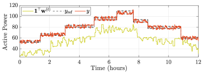
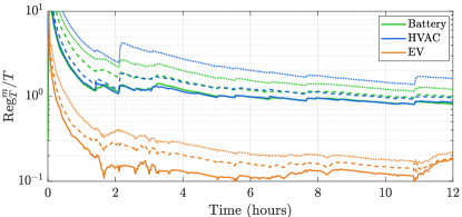
Refer to caption
Refer to caption
Figure 4: (a) Tracking of yrefsubscript𝑦refy_{\mathrm{ref}} by the GP-based online primal-dual method and (b) Local network regret (solid line corresponds to true {Um,n}subscript𝑈𝑚𝑛\{U_{m,n}\}, dashed line to estimate {U^m,n}subscript^𝑈𝑚𝑛\{\hat{U}_{m,n}\} via shape-constrained GPs, and dotted line to estimate {U^m,n}subscript^𝑈𝑚𝑛\{\hat{U}_{m,n}\} via GPs).
Refer to caption
Figure 5: Disagreement between system and users (zoom for the first hour of simulation where each user is represented by a different line style). The primal variables xmsubscript𝑥𝑚x_{m} and xm,nsubscript𝑥𝑚𝑛x_{m,n} are normalized such that 102superscript10210^{-2} corresponds to 1%percent11\% error.
Refer to caption
Figure 6: Behavior of the setpoint x3subscript𝑥3x_{3} and the desirable setpoint for the user x3,1subscript𝑥31x_{3,1}, compared with the optimal solution x3superscriptsubscript𝑥3x_{3}^{*}
Refer to caption
Figure 7: Behavior of ξtsuperscript𝜉𝑡\xi^{t} and ΞtsuperscriptΞ𝑡\Xi^{t} over time.
Refer to caption
Figure 8: Global network regret for different values of δ𝛿\delta.
Refer to caption
Figure 9: Global network regret over time under different load profiles.
Refer to caption
Figure 10: Global network regret for different values of M𝑀M and Nmaxsubscript𝑁maxN_{\mathrm{max}} (solid line corresponds to true {Um,n}subscript𝑈𝑚𝑛\{U_{m,n}\}, dashed line to estimate {U^m,n}subscript^𝑈𝑚𝑛\{\hat{U}_{m,n}\} via shape-constrained GPs).

VI Conclusions

In this work, we presented an online consensus-based algorithm to solve a time-varying optimization problem associated with a network of systems shared by multiple users. The cost function that represents the individuals’ preferences were learned concurrently with the execution of the algorithm via shape-constrained GPs using users’ feedback. We developed an online algorithm based on a primal-dual method, properly modified to accommodate feedback from the users and measurements from the network. We analyzed the performance via dynamic network regret and average constraint violation, and we showed that the bounds of these metrics depend on the temporal variability of the optimal solution set, and the errors associated with the estimation of the gradients. Numerical results were presented in the context of real-time management of distributed energy resources. Future efforts include investigating the convergence of multi-time-scale algorithms, and the case where the users’ cost functions are time-varying to reflect preferences that change over time.

References

  • [1] J. Koshal, A. Nedić, and U. V. Shanbhag, “Multiuser optimization: Distributed algorithms and error analysis,” SIAM Journal on Optimization, vol. 21, no. 3, pp. 1046–1081, 2011.
  • [2] B. Turan, C. A. Uribe, H. T. Wai, and M. Alizadeh, “Resilient primal–dual optimization algorithms for distributed resource allocation,” IEEE Transactions on Control of Network Systems, vol. 8, no. 1, pp. 282–294, 2021.
  • [3] A. Y. Popkov, “Gradient methods for nonstationary unconstrained optimization problems,” Automation and Remote Control, vol. 66, no. 6, pp. 883–891, 2005.
  • [4] A. Simonetto and G. Leus, “Double smoothing for time-varying distributed multiuser optimization,” in IEEE Global Conf. on Signal and Information Processing, Dec. 2014.
  • [5] M. Fazlyab, C. Nowzari, G. J. Pappas, A. Ribeiro, and V. M. Preciado, “Self-triggered time-varying convex optimization,” in IEEE Conference on Decision and Control, 2016, pp. 3090–3097.
  • [6] A. Simonetto, E. Dall’Anese, S. Paternain, G. Leus, and G. B. Giannakis, “Time-varying convex optimization: Time-structured algorithms and applications,” Proceedings of the IEEE, vol. 108, no. 11, pp. 2032–2048, 2020.
  • [7] A. Bajcsy, A. Siththaranjan, C. J. Tomlin, and A. D. Dragan, “Analyzing human models that adapt online,” in 2021 IEEE International Conference on Robotics and Automation (ICRA), 2021, pp. 2754–2760.
  • [8] N. Lassen, F. Goia, S. Schiavon, and J. Pantelic, “Field investigations of a smiley-face polling station for recording occupant satisfaction with indoor climate,” Building and Environment, vol. 185, p. 107266, 2020.
  • [9] B. Lepri, J. Staiano, D. Sangokoya, E. Letouzé, and N. Oliver, “The tyranny of data? The bright and dark sides of data-driven decision-making for social good,” in Transparent data mining for big and small data.   Springer, 2017, pp. 3–24.
  • [10] X. Wang and J. O. Berger, “Estimating shape constrained functions using Gaussian Processes,” SIAM/ASA Journal on Uncertainty Quantification, vol. 4, no. 1, pp. 1–25, 2016.
  • [11] S. Bolognani and S. Zampieri, “A distributed control strategy for reactive power compensation in smart microgrids,” IEEE Transactions on Automatic Control, vol. 58, no. 11, pp. 2818–2833, 2013.
  • [12] A. Bernstein, E. Dall’Anese, and A. Simonetto, “Online primal-dual methods with measurement feedback for time-varying convex optimization,” IEEE Transactions on Signal Processing, vol. 67, no. 8, pp. 1978–1991, 2019.
  • [13] Q. Wang, M. Liu, and J. L. Mathieu, “Adaptive demand response: Online learning of restless and controlled bandits,” in 2014 IEEE International Conference on Smart Grid Communications, 2014, pp. 752–757.
  • [14] A. Lesage-Landry and D. S. Callaway, “Dynamic and distributed online convex optimization for demand response of commercial buildings,” IEEE Control Systems Letters, 2020.
  • [15] T. Chen, B. Zhang, H. Pourbabak, A. Kavousi-Fard, and W. Su, “Optimal routing and charging of an electric vehicle fleet for high-efficiency dynamic transit systems,” IEEE Transactions on Smart Grid, vol. 9, no. 4, pp. 3563–3572, 2018.
  • [16] X. Luo, Y. Zhang, and M. M. Zavlanos, “Socially-aware robot planning via bandit human feedback,” in 2020 ACM/IEEE 11th International Conference on Cyber-Physical Systems (ICCPS), 2020, pp. 216–225.
  • [17] A. Koppel, F. Jakubeic, and A. Ribeiro, “A saddle point algorithm for networked online convex optimization,” IEEE Transactions on Signal Processing, vol. 63, no. 19, pp. 5149–5164, 10 2015.
  • [18] S. Lee and M. M. Zavlanos, “Distributed primal-dual methods for online constrained optimization,” in 2016 American Control Conference (ACC).   IEEE, 2016, pp. 7171–7176.
  • [19] T. Chen and G. B. Giannakis, “Bandit convex optimization for scalable and dynamic IoT management,” IEEE Internet of Things Journal, vol. 6, no. 1, pp. 1276–1286, 2018.
  • [20] E. C. Hall and R. M. Willett, “Online convex optimization in dynamic environments,” IEEE Journal of Selected Topics in Signal Processing, vol. 9, no. 4, pp. 647–662, 2015.
  • [21] S. Shahrampour and A. Jadbabaie, “Distributed Online Optimization in Dynamic Environments Using Mirror Descent,” IEEE Transactions on Automatic Control, vol. 63, no. 3, pp. 714 – 725, 2018.
  • [22] T. Yang, L. Zhang, R. Jin, and J. Yi, “Tracking slowly moving clairvoyant: Optimal dynamic regret of online learning with true and noisy gradient,” in International Conference on Machine Learning, 2016.
  • [23] A. D. Flaxman, A. T. Kalai, and H. B. McMahan, “Online convex optimization in the bandit setting: Gradient descent without a gradient,” in 16th Annual ACM-SIAM Symposium on Discrete Algorithms.   SIAM, 2005, p. 385–394.
  • [24] J. Li, C. Gu, Z. Wu, and T. Huang, “Online learning algorithm for distributed convex optimization with time-varying coupled constraints and bandit feedback,” IEEE Transactions on Cybernetics, vol. 52, no. 2, pp. 1009–102, 2022.
  • [25] Y. Tang, Z. Ren, and N. Li, “Zeroth-order feedback optimization for cooperative multi-agent systems,” in 2020 59th IEEE Conference on Decision and Control (CDC), 2020, pp. 3649–3656.
  • [26] S. Liu, P.-Y. Chen, B. Kailkhura, G. Zhang, A. O. Hero III, and P. K. Varshney, “A primer on zeroth-order optimization in signal processing and machine learning: Principals, recent advances, and applications,” IEEE Signal Processing Magazine, vol. 37, no. 5, pp. 43–54, 2020.
  • [27] N. Srinivas, A. Krause, S. M. Kakade, and M. W. Seeger, “Information-Theoretic Regret Bounds for Gaussian Process Optimization in the Bandit Setting,” IEEE Transactions on Information Theory, vol. 58, no. 5, pp. 3250 – 3265, 2012.
  • [28] I. Notarnicola, A. Simonetto, F. Farina, and G. Notarstefano, “Distributed personalized gradient tracking with convex parametric models,” IEEE Transactions on Automatic Control, 2022.
  • [29] A. Simonetto, E. Dall’Anese, J. Monteil, and A. Bernstein, “Personalized optimization with user’s feedback,” Automatica, vol. 131, 2021.
  • [30] A. M. Ospina, A. Simonetto, and E. Dall’Anese, “Personalized demand response via shape-constrained online learning,” in 2020 IEEE International Conference on Communications, Control, and Computing Technologies for Smart Grids (SmartGridComm), 2020, pp. 1–6.
  • [31] C. E. Rasmussen, “Gaussian processes for machine learning,” in Gaussian processes for machine learning.   MIT Press, 2006.
  • [32] D. P. Bertsekas and J. N. Tsitsiklis, “Gradient convergence in gradient methods with errors,” SIAM Journal on Optimization, vol. 10, no. 3, pp. 627–642, 2000.
  • [33] R. M. Gower, N. Loizou, X. Qian, A. Sailanbayev, E. Shulgin, and P. Richtárik, “SGD: General analysis and improved rates,” in International Conference on Machine Learning.   PMLR, 2019, pp. 5200–5209.
  • [34] X. Yi, X. Li, L. Xie, and K. H. Johansson, “Distributed online convex optimization with time-varying coupled inequality constraints,” IEEE Transactions on Signal Processing, vol. 68, pp. 731–746, 2020.