Abstract

The electroweak (EW) sector of the Minimal Supersymmetric Standard Model (MSSM) can account for variety of experimental data. In particular it can explain the persistent $3-4\,\sigma$ discrepancy between the experimental result for the anomalous magnetic moment of the muon, $(g-2)_{\mu}$, and its Standard Model (SM) prediction. The lighest supersymmetric particle (LSP), which we take as the lightest neutralino, $\tilde{\chi}_{1}^{0}$, can furthermore account for the observed Dark Matter (DM) content of the universe via coannihilation with the next-to-LSP (NLSP), while being in agreement with negative results from Direct Detection (DD) experiments. Concerning the unsuccessful searches for EW particles at the LHC, owing to relatively small production cross-sections a comparably light EW sector of the MSSM is in full agreement with the experimental data. The DM relic density can fully be explained by a mixed bino/wino LSP. Here we take the relic density as an upper bound, which opens up the possibility of wino and higgsino DM. We first analyze which mass ranges of neutralinos, charginos and scalar leptons are in agreement with all experimental data, including relevant LHC searches. We find roughly an upper limit of $\sim 600\,\,\mathrm{GeV}$ for the LSP and NLSP masses. In a second step we assume that the new result of the Run 1 of the “MUON G-2” collaboration at Fermilab yields a precision comparable to the existing experimental result with the same central value. We analyze the potential impact of the combination of the Run 1 data with the existing $(g-2)_{\mu}$ data on the allowed MSSM parameter space. We find that in this case the upper limits on the LSP and NLSP masses are substantially reduced by roughly $100\,\,\mathrm{GeV}$. We interpret these upper bounds in view of future HL-LHC EW searches as well as future high-energy $e^{+}e^{-}$ colliders, such as the ILC or CLIC.

1 Introduction

One of the most important tasks at the LHC is to search for physics beyond the Standard Model (SM). This includes the production and measurement of the properties of Cold Dark Matter (CDM). These two (related) tasks will be among the top priority in the future program of high-energy particle physics. One tantalizing hint for physics beyond the SM (BSM) is the anomalous magnetic moment of the muon, $(g-2)_{\mu}$. The experimental result deviates from the SM prediction by $3-4\sigma$ [1, 2]. Improved experimental results are expected soon [3] from the Run 1 data of the “MUON G-2” experiment [4]. Another clear sign for BSM physics is the precise measurement of the CDM relic abundance [5]. A final set of related constraints comes from CDM Direct Detection (DD) experiments. The LUX [6], PandaX-II [7] and XENON1T [8] experiments provide stringent limits on the spin-independent (SI) DM scattering cross-section, $\sigma_{p}^{\rm SI}$.

Among the BSM theories under consideration the Minimal Supersymmetric Standard Model (MSSM) [9, 10, 11, 12] is one of the leading candidates. Supersymmetry (SUSY) predicts two scalar partners for all SM fermions as well as fermionic partners to all SM bosons. Contrary to the case of the SM, in the MSSM two Higgs doublets are required. This results in five physical Higgs bosons instead of the single Higgs boson in the SM. These are the light and heavy ${{\cal CP}}$-even Higgs bosons, $h$ and $H$, the ${{\cal CP}}$-odd Higgs boson, $A$, and the charged Higgs bosons, $H^{\pm}$. The neutral SUSY partners of the (neutral) Higgs and electroweak gauge bosons gives rise to the four neutralinos, $\tilde{\chi}_{1,2,3,4}^{0}$. The corresponding charged SUSY partners are the charginos, $\tilde{\chi}_{1,2}^{\pm}$. The SUSY partners of the SM leptons and quarks are the scalar leptons and quarks (sleptons, squarks), respectively.

The electroweak (EW) sector of the MSSM (the charginos, neutralinos and scalar leptons) can account for a variety of experimental data. The lightest SUSY particle (LSP), the lightest neutralino $\tilde{\chi}_{1}^{0}$, can explain the CDM relic abundance [13, 14], while not being in conflict with negative DD results and the negative LHC searches. The requirement to give the full amount of DM relic density can be met if the LSP is a bino or a mixed bino/wino state. Furthermore, the EW sector of the MSSM can account for the persistent $3-4\,\sigma$ discrepancy of $(g-2)_{\mu}$. Recently in Ref. [15], assuming that the LSP gives rise to the full amount of DM relic density, upper limits on the various masses of the EW SUSY sector were derived, while being in agreement with all other experimental data. The upper limits strongly depend on the deviation of the experimental result of $(g-2)_{\mu}$ from its SM prediction. Taking the current deviation of $(g-2)_{\mu}$ [1, 2], limits of roughly $\sim 600\,\,\mathrm{GeV}$ were set on the mass of the LSP and the next-to-LSP (NLSP). Assuming that the new result of the Run 1 of the “MUON G-2” collaboration at Fermilab yields a precision comparable to the existing experimental result with the same central value, yielded a reduction of these upper limits of roughly $\sim 100\,\,\mathrm{GeV}$.

In this paper we perform an analysis similar to [15], but under the assumption that the relic DM only gives an upper bound, which opens up the possibility of wino and higgsino DM. We analyze the four cases of bino-dominated, bino/wino, (nearly pure) wino and higgsino LSP for the current deviation of $(g-2)_{\mu}$, as well as for the assumption of improved $(g-2)_{\mu}$ bounds from the combination of existing experimental data with the Run 1 data of the “MUON G-2” experiment. In all cases we require the agreement with all other relevant existing data, such as the DD bounds and the EW searches at the LHC. The derived upper limits on the EW masses are discussed in the context of the upcoming searches at the HL-LHC as well as at possible future $e^{+}e^{-}$ colliders, such as the ILC [36, 37] or CLIC [38, 37].

2 The electroweak sector of the MSSM

In our notation for the MSSM we follow exactly Ref. [15]. Here we retrict ourselves to a very short introduction of the relevant parameters and symbols of the EW sector of the MSSM, consisting of charginos, neutralinos and scalar leptons. The scalar quark sector is assumed to be heavy and not to play a relevant role in our analysis. Throughout this paper we also assume that all parameters are real, i.e. the absence of ${\cal CP}$-violation.

The masses and mixings of the neutralinos are determined (besides SM parameters)) by $U(1)_{Y}$ and $SU(2)_{L}$ gaugino masses $M_{1}$ and $M_{2}$, the Higgs mixing parameter $\mu$ and $\tan\beta$, the ratio of the two vacuum expectation values (vevs) of the two Higgs doublets of MSSM, $\tan\beta=v_{2}/v_{1}$. After diagonalization, the four eigenvalues of the matrix give the four neutralino masses $m_{\tilde{\chi}_{1}^{0}}<m_{\tilde{\chi}_{2}^{0}}<m_{\tilde{\chi}_{3}^{0}}<m_{\tilde{\chi}_{4}^{0}}$. The masses and mixings of the charginos are determined (besides SM parameters) by $M_{2}$, $\mu$ and $\tan\beta$. Diagonalizing the mass matrix two chargino-mass eigenvalues $m_{\tilde{\chi}_{1}^{\pm}}<m_{\tilde{\chi}_{2}^{\pm}}$ can be obtained.

For the sleptons, as in Ref. [15], we choose common soft SUSY-breaking parameters for all three generations. The charged slepton mass matrix are determined (besides SM parameters) by the diagonal soft SUSY-breaking parameters $m_{\tilde{l}_{L}}^{2}$ and $m_{\tilde{l}_{R}}^{2}$ and the trilinear coupling $A_{l}$ ($l=e,\mu,\tau$), where the latter are taken to be zero. Mixing between the “left-handed” and “right-handed” sleptons is only relevant for scalar taus, where the off-diagonal entry in the mass matrix is given by $-m_{\tau}\mu\tan\beta$. Thus, for the first two generations, the mass eigenvalues can be approximated as $m_{\tilde{l}_{1}}\simeq m_{\tilde{l}_{L}},m_{\tilde{l}_{2}}\simeq m_{\tilde{l}_{R}}$. In general we follow the convention that $\tilde{l}_{1}$ ($\tilde{l}_{2}$) has the large “left-handed” (“right-handed”) component. Besides the symbols equal for all three generations, we also explicitly use the scalar electron, muon and tau masses, $m_{\tilde{e}_{1,2}}$, $m_{\tilde{\mu}_{1,2}}$ and $m_{\tilde{\tau}_{1,2}}$. The sneutrino and slepton masses are connected by the usual SU(2) relation.

Overall, the EW sector at the tree level can be described with the help of six parameters: $M_{1},M_{2},\mu,\tan\beta,m_{\tilde{l}_{L}},m_{\tilde{l}_{R}}$. Throughout our analysis we neglect ${{\cal CP}}$-violation and assume $\mu,M_{1},M_{2}>0$. In Ref. [15] it was shown that choosing these parameters positive covers the relevant parameter space once the $(g-2)_{\mu}$ results are taken into account (see, however, the discussion in Sect. 7).

Following the stronger experimental limits from the LHC [39, 40], we assume that the colored sector of the MSSM is sufficiently heavier than the EW sector, and does not play a role in this analysis. For the Higgs-boson sector we assume that the radiative corrections to the light ${{\cal CP}}$-even Higgs boson (largely originating from the top/stop sector) yield a value in agreement with the experimental data, $M_{h}\sim 125\,\,\mathrm{GeV}$. This naturally yields stop masses in the TeV range [41, 42], in agreement with the above assumption. Concerning the Higgs-boson mass scale, as given by the ${{\cal CP}}$-odd Higgs-boson mass, $M_{A}$, we employ the existing experimental bounds from the LHC. In the combination with other data, this results in a mostly non-relevant impact of the heavy Higgs bosons on our analysis, as will be discussed below.

3 Relevant constraints

The experimental result for $a_{\mu}:=(g-2)_{\mu}/2$ is dominated by the measurements made at the Brookhaven National Laboratory (BNL) [43], resulting in a world average of [44]

$$a_{\mu}^{\rm exp} =11659209.1(5.4)(3.3)\times 10^{-10}\leavevmode\nobreak\ ,$$ (1)

where the first uncertainty is statistical and the second systematic. The SM prediction of $a_{\mu}$ is given by [45] (based on Refs. [46, 47, 48, 49, 50, 51, 52, 53, 2, 1, 54, 55, 56, 57, 58, 59, 60, 61, 62, 63] ),

$$a_{\mu}^{\rm SM} =(11659181.0\pm 4.3)\times 10^{-10}\leavevmode\nobreak\ .$$ (2)

Comparing this with the current experimental measurement in Eq. (1) results in a deviation of

$$\Delta a_{\mu}^{\rm old} =(28.1\pm 7.6)\times 10^{-10}\leavevmode\nobreak\ ,$$ (3)

corresponding to a $3.7\,\sigma$ discrepancy. This “current” result will be used below with a hard cut at $2\,\sigma$ uncertainty.

Efforts to improve the experimental result at Fermilab by the “MUON G-2” collaboration [4] and at J-PARC [64] aim to reduce the experimental uncertainty by a factor of four compared to the BNL measurement. For the second step in our analysis we consider the upcoming Run 1 result from the Fermilab experiment [3]. The Run 1 data is expected to have roughly the same experimental uncertainty as the current result in Eq. (1). We furthermore assume that the Run 1 data yields the same central value as the current result. Consequently, we anticipate that the experimental uncertainty shrinks by $1/\sqrt{2}$, yielding a future value of

$$\Delta a_{\mu}^{\rm fut} =(28.1\pm 6.2)\times 10^{-10}\leavevmode\nobreak\ ,$$ (4)

corresponding to a $4.5\,\sigma$ discrepancy. Thus, the combination of Run 1 data with the existing experimental $(g-2)_{\mu}$ data has the potential to (nearly) establish the “discovery” of BSM physics. This “anticipated future” result will be used below with a hard cut at $2\,\sigma$ uncertainty.

Recently a new lattice calculation for the leading order hadronic vacuuum polarization (LO HVP) contribution to $a_{\mu}^{\rm SM}$ [65] has been reported, which, however, was not used in the new theory world average, Eq. (2) [45]. Consequently, we also do not take this result into account, see also the discussions in Ref. [15, 66, 65, 67, 68, 69]. On the other hand, we are also aware that our conclusions would change substantially if the result presented in [65] turned out to be correct.

In the MSSM the main contribution to $(g-2)_{\mu}$ at the one-loop level comes from diagrams involving $\tilde{\chi}_{1}^{\pm}-\tilde{\nu}$ and $\tilde{\chi}_{1}^{0}-\tilde{\mu}$ loops. In the case of a bino-dominated LSP the contributions are approximated as [70, 71, 72]

$$a^{\tilde{\chi}^{\pm}-\tilde{\nu}_{\mu}}_{\mu} \approx \frac{\alpha\,m^{2}_{\mu}\,\mu\,M_{2}\tan\beta}{4\pi\sin^{2}\theta_{W}\,m_{\tilde{\nu}_{\mu}}^{2}}\left(\frac{f_{\chi^{\pm}}(M_{2}^{2}/m_{\tilde{\nu}_{\mu}}^{2})-f_{\chi^{\pm}}(\mu^{2}/m_{\tilde{\nu}_{\mu}}^{2})}{M_{2}^{2}-\mu^{2}}\right)\,,$$ (5)

$$a^{\tilde{\chi}^{0}-\tilde{\mu}}_{\mu} \approx \frac{\alpha\,m^{2}_{\mu}\,\,M_{1}(\mu\tan\beta-A_{\mu})}{4\pi\cos^{2}\theta_{W}\,(m_{\tilde{\mu}_{R}}^{2}-m_{\tilde{\mu}_{L}}^{2})}\left(\frac{f_{\chi^{0}}(M^{2}_{1}/m_{\tilde{\mu}_{R}}^{2})}{m_{\tilde{\mu}_{R}}^{2}}-\frac{f_{\chi^{0}}(M^{2}_{1}/m_{\tilde{\mu}_{L}}^{2})}{m_{\tilde{\mu}_{L}}^{2}}\right)\,,$$ (6)

where the loop functions $f$ are as given in Ref. [72]. In our analysis MSSM contribution to $(g-2)_{\mu}$ up to two-loop order is calculated using GM2Calc [73], implementing two-loop corrections from [74, 75, 76] (see also [77, 78]). This code also works numerically reliable for the cases of (very) compressed spectra, such as for wino and higgsino DM.

Other constraints

All other experimental constraints are taken into account exactly as in Ref. [15]. These comprise

• Vacuum stability constraints:
  All points are check to possess a stable and correct EW vacuum, e.g. avoiding charge and color breaking minima. This check is performed with the public code Evade [79, 80].

• Constraints from the LHC:
  All relevant EW SUSY searches are taken into account, mostly via CheckMATE [81, 82, 83], where many analysis had to be implemented newly [15]. As in Ref. [15], the constraints coming from "compressed spectra" searches [84], corresponding to very low splittings between $m_{\tilde{\chi}_{1}^{\pm}},m_{\tilde{\chi}_{2}^{0}},m_{\tilde{l}_{1}}$ and $m_{\tilde{\chi}_{1}^{0}}$ are applied directly on our parameter space.

  In addition to the searches described in Ref. [15], we take into account the latest constraints from the disappearing track searches at the LHC [85, 86]. These are particularly important for wino DM scenario where the mass gap between $\tilde{\chi}_{1}^{\pm}$ and $\tilde{\chi}_{1}^{0}$ can be $\sim$ a few hundred $\,\,\mathrm{MeV}$. The long-lived $\tilde{\chi}_{1}^{\pm}$ (lifetime $\sim{\cal O}(\mathrm{ns})$) decays into final states involving a $\tilde{\chi}_{1}^{0}$ and a soft pion which can not be reconstructed within the detector. Thus, the signal involves a charged track from $\tilde{\chi}_{1}^{\pm}$ that produces hits only in the innermost layers of the detector with no subsequent hits at larger radii.

• Dark matter relic density constraints:
  We use the latest result from Planck [5].

  $$\Omega_{\rm CDM}h^{2}\;\leq\;0.122,$$ (7)

  As stressed above, we take the relic density as an upper limit (evaluated from the central value plus $2\,\sigma$. The relic density in the MSSM is evaluated with MicrOMEGAs [87, 88, 89, 90]. An additional DM component could be, e.g., a SUSY axion [91], which would then bring the total DM density into agreement with the Planck measurement of $\Omega_{\rm CDM}h^{2}=0.120\pm 0.001$ [5].

  In the case of wino DM, because of the extremely small mass splitting, the effect of “Sommerfeld enhancement” [92] can be very important. For wino DM providing the full amount of DM it shifts the allowed range of $m_{\tilde{\chi}_{1}^{0}}$ from $\sim 2.0\,\,\mathrm{TeV}$ to about $\sim 2.9\,\,\mathrm{TeV}$. Since here we are interested in the case that the wino DM only gives a fraction of the whole DM relic density, see Eq. (7), we can safely neglect the Sommerfeld enhancement. The upper limit on $m_{\tilde{\chi}_{1}^{0}}$ is given, as will be shown below, by the $(g-2)_{\mu}$ constraint, but not by the DM relic density. Allowing higher masses here (as would be the case if the Sommerfeld enhancement had been taken into account) could thus not lead to a larger allowed parameter space. On the other hand, for a point with a relic density fulfilling Eq. (7) the Sommerfeld enhancement would only lower the “true” DM density, which still fulfills Eq. (7).

• Direct detection constraints of Dark matter:
  We employ the constraint on the spin-independent DM scattering cross-section $\sigma_{p}^{\rm SI}$ from XENON1T [8] experiment, evaluating the theoretical prediction for $\sigma_{p}^{\rm SI}$ using MicrOMEGAs [87, 88, 89, 90]. A combination with other DD experiments would yield only very slightly stronger limits, with a negligible impact on our results. For parameter points with $\Omega_{\tilde{\chi}}h^{2}\;\leq\;0.118$ ($2\,\sigma$ lower limit from Planck [5]), we scale the cross-section with a factor of ($\Omega_{\tilde{\chi}}h^{2}$/0.118) to account for the fact that $\tilde{\chi}_{1}^{0}$ provides only a fraction of the total DM relic density of the universe. Here the effect of neglecting the Sommerfeld enhancement leads to a more conservative allowed region of parameter space.

4 Parameter scan and analysis flow

4.1 Parameter scan

We scan the relevant MSSM parameter space to obtain lower and upper limits on the relevant neutralino, chargino and slepton masses. In order to achieve a “correct” DM relic density, see Eq. (7), by the lightest neutralino, $\tilde{\chi}_{1}^{0}$, some mechanism such as a specific co-annihilation or pole annihilation has to be active in the early universe. At the same time $m_{\tilde{\chi}_{1}^{0}}$ must not be too high, such that the EW sector can provide the contribution required to bring the theory prediction of $a_{\mu}$ into agreement with the experimental measurement, see Sect. 3. The combination of these two requirements yields the following possibilities. (The cases present a certain choice of favored possibilities, upon which one can expand, as will briefly discussed in Sect. 7.)

(A) Higgsino DM
This scenario is characterized by a small value of $\mu$ (as favored, e.g., by naturalness arguments [93, 94, 95, 96, 97, 98]). Such a scenario is also naturally realized in Anomaly Mediation SUSY breaking (see e.g. Ref. [100] and references therein). We scan the following parameters:

$$100\,\,\mathrm{GeV}\leq\mu\leq 1.2\,\,\mathrm{TeV}\;,\quad 1.1\mu\leq M_{1}\leq 10\mu\;,$$

$$\quad 1.1\mu\leq M_{2}\leq 10\mu,\;\quad 5\leq\tan\beta\leq 60,\;$$

$$\quad 100\,\,\mathrm{GeV}\leq m_{\tilde{l}_{L}},m_{\tilde{l}_{R}}\leq 2\,\,\mathrm{TeV}\leavevmode\nobreak\ .$$ (8)

(B) Wino DM
This scenario is characterized by a small value of $M_{2}$. Such a scenario is also naturally realized in Anomaly Mediation SUSY breaking (see e.g. Ref. [100] and references therein). We scan the following parameters:

$$100\,\,\mathrm{GeV}\leq M_{2}\leq 1.5\,\,\mathrm{TeV}\;,\quad 1.1M_{2}\leq M_{1}\leq 10M_{2}\;,$$

$$\quad 1.1M_{2}\leq\mu\leq 10M_{2},\;\quad 5\leq\tan\beta\leq 60,\;$$

$$\quad 100\,\,\mathrm{GeV}\leq m_{\tilde{l}_{L}},m_{\tilde{l}_{R}}\leq 2\,\,\mathrm{TeV}\leavevmode\nobreak\ .$$ (9)

The choice of $M_{2}\ll M_{1},\mu$ leads (at tree-level) to a very degenerate spectrum with $m_{\tilde{\chi}_{1}^{\pm}}-m_{\tilde{\chi}_{1}^{0}}={\cal O}(1{\rm\,eV})$. However, this spectrum does not correspond to the on-shell (OS) masses of all six charginos and neutralinos. Since only three (soft SUSY-breaking) mass parameters are available ($M_{1}$, $M_{2}$ and $\mu$), only three out of the six masses can be renormalized OS. The (one-loop) shifts for the three remaining masses are obtained via the CCN_i renormalization scheme [101] with $i\in\{2,3,4\}$. In a CCN_i scheme the $\tilde{\chi}_{1}^{\pm}$, $\tilde{\chi}_{2}^{\pm}$ and $\tilde{\chi}_{i}^{0}$ are chosen OS. This automatically yields a good renormalization for $M_{2}$ and $\mu$. The $\tilde{\chi}_{i}^{0}$ has to be chosen, parameter point by parameter point, such that also $M_{1}$ is renormalized well (which excludes the CCN₁ for $M_{2}\ll M_{1},\mu$). For each point we choose the $\tilde{\chi}_{i}^{0}$ to be renormalized OS such that the maximum shift of all three shifted neutralino masses is minimized. We have explicitly checked for each scanned point that the such chosen CCN_i indeed yields reasonably small shifts for three shifted neutralino masses, in particular for $m_{\tilde{\chi}_{1}^{0}}$. Only this transition to OS masses yields a mass splitting between $m_{\tilde{\chi}_{1}^{\pm}}$ and $m_{\tilde{\chi}_{1}^{0}}$ that allows then for the decay $\tilde{\chi}_{1}^{\pm}\to\tilde{\chi}_{1}^{0}\pi^{\pm}$.

(C) Mixed bino/wino DM
This scenario has been analyzed in Ref. [15]. It can in principle be realized in three different versions corresponding to the coannihilation mechanism (see Ref. [15] for a detailed discussion). However, a larger wino component is found only for $\tilde{\chi}_{1}^{\pm}$-coannihilation. The scan parameters are chosen as,

$$100\,\,\mathrm{GeV}\leq M_{1}\leq 1\,\,\mathrm{TeV}\;,\quad M_{1}\leq M_{2}\leq 1.1M_{1}\;,$$

$$\quad 1.1M_{1}\leq\mu\leq 10M_{1},\;\quad 5\leq\tan\beta\leq 60,\;$$

$$\quad 100\,\,\mathrm{GeV}\leq m_{\tilde{l}_{L}}\leq 1.5\,\,\mathrm{TeV},\;\quad m_{\tilde{l}_{R}}=m_{\tilde{l}_{L}}\leavevmode\nobreak\ .$$ (10)

Here we choose one soft SUSY-breaking parameter for all sleptons together. While this choice should not have a relevant effect in the $\tilde{\chi}_{1}^{\pm}$-coannihilation case, this have an impact in the next case. In our scans we will see that the chosen lower and upper limits are not reached by the points that meet all the experimental constraints. This ensures that the chosen intervals indeed cover all the relevant parameter space.

(D) Bino DM
This scenario covers the coannihilation with sleptons, and has also been analyzed in Ref. [15]. In this scenario “accidentally” the wino component of the $\tilde{\chi}_{1}^{0}$ can be non-negligible. However, this is not a distinctive feature of this scenario. We cover the two distinct cases that either the SU(2) doublet sleptons, or the singlet sleptons are close in mass to the LSP.
(D1) Case-L: SU(2) doublet

$$100\,\,\mathrm{GeV}\leq M_{1}\leq 1\,\,\mathrm{TeV}\;,\quad M_{1}\leq M_{2}\leq 10M_{1}\;,$$

$$\quad 1.1M_{1}\leq\mu\leq 10M_{1},\;\quad 5\leq\tan\beta\leq 60,\;$$

$$\quad M_{1}\,\,\mathrm{GeV}\leq m_{\tilde{l}_{L}}\leq 1.2M_{1},\quad M_{1}\leq m_{\tilde{l}_{R}}\leq 10M_{1}\leavevmode\nobreak\ .$$ (11)

(D2) Case-R: SU(2) singlet

$$100\,\,\mathrm{GeV}\leq M_{1}\leq 1\,\,\mathrm{TeV}\;,\quad M_{1}\leq M_{2}\leq 10M_{1}\;,$$

$$\quad 1.1M_{1}\leq\mu\leq 10M_{1},\;\quad 5\leq\tan\beta\leq 60,\;$$

$$\quad M_{1}\,\,\mathrm{GeV}\leq m_{\tilde{l}_{R}}\leq 1.2M_{1},\;\quad M_{1}\leq m_{\tilde{l}_{L}}\leq 10M_{1}\leavevmode\nobreak\ .$$ (12)

In all scans we choose flat priors of the parameter space and generate ${\cal O}(10^{7})$ points.

The mass parameters of the colored sector have been set to high values, such that the resulting SUSY particle masses are outside the reach of the LHC, the light ${{\cal CP}}$-even Higgs-boson is in agreement with the LHC measurements (see, e.g., Refs. [41, 42]), where the concrete values are not relevant for our analysis. $M_{A}$ has also been set to be above the TeV scale. Consequently, we do not include explicitly the possibility of $A$-pole annihilation, with $M_{A}\sim 2m_{\tilde{\chi}_{1}^{0}}$. As we will discuss below the combination of direct heavy Higgs-boson searches with the other experimental requirements constrain this possibility substantially (see, however, also Sect. 6). Similarly, we do not consider $h$- or $Z$-pole annihilation, as such a light neutralino sector likely overshoots the $(g-2)_{\mu}$ contribution (see, however, the discussion in Sect. 6).

4.2 Analysis flow

The data sample is generated by scanning randomly over the input parameter range mentioned above, using a flat prior for all parameters. We use SuSpect [103] as spectrum and SLHA file generator, which yields $\smash{\overline{\mathrm{DR}}}$ values for the chargino and neutralino masses. While in most of the cases the difference between $\smash{\overline{\mathrm{DR}}}$ and on-shell (OS) masses is not phenomenologically relevant for our analysis, this is different for wino DM. Because of the very small mass difference of the $\smash{\overline{\mathrm{DR}}}$ values for $m_{\tilde{\chi}_{1}^{0}}$ and $m_{\tilde{\chi}_{1}^{\pm}}$ we take into account the transition to OS masses, as discussed above. In the next step the points are required to satisfy the $\tilde{\chi}_{1}^{\pm}$ mass limit from LEP [104]. The SLHA output files from SuSpect are then passed as input to GM2Calc and MicrOMEGAs for the calculation of $(g-2)_{\mu}$ and the DM observables, respectively. The parameter points that satisfy the current $(g-2)_{\mu}$ constraint, Eq. (3), the DM relic density, Eq. (7), the direct detection constraints and the vacuum stability constraints as checked with Evade are then taken to the final step to be checked against the latest LHC constraints implemented in CheckMATE.  The branching ratios of the relevant SUSY particles are computed using SDECAY [105] and given as input to CheckMATE.

5 Results

5.1 Higgsino DM

We start our discussion with the case of higgsino DM, as discussed in Sect. 4.1. We follow the analysis flow as described in Sect. 4.2, where the vacuum stability constraints did not affect any of the LHC allowed points. We also remark that we have checked that the (possible) one-loop corrections to the chargino/neutralino masses do not change the results in a relevant way and were thus omitted (see, however, Sect. 5.2). In the following we denote the points surviving certain constraints with different colors:

• grey (round): all scan points (i.e. points excluded by $(g-2)_{\mu}$).

• green (round): all points that are in agreement with $(g-2)_{\mu}$, taking into account the current or anticipated future limits, see Eqs. (3) and (4), respectively, (i.e. points excluded by the DM relic density).

• blue (triangle): points that additionally obey the upper limit of the DM relic density, see Eq. (7) (i.e. points excluded by the DD constraints). In some plots below all points that pass the $(g-2)_{\mu}$ constraint are also in agreement with the DM relic density constraint, resulting in only blue (but no green) points to be visible.

• cyan (diamond): points that additionally pass the DD constraints, see Sect. 3 (i.e. points excluded by the LHC constraints).

• red (star): points that additionally pass the LHC constraints, see Sect. 3 (i.e. points that pass all constraints).

In Fig. 1 we show our results in the $m_{\tilde{\chi}_{1}^{0}}$–$m_{\tilde{\chi}_{1}^{\pm}}$ plane for the current (left) and future (right) $(g-2)_{\mu}$ constraint, see Eqs. (3) and (4), respectively. By definition the points are clustered in the diagonal of the plane, and $m_{\tilde{\chi}_{2}^{0}}\approx m_{\tilde{\chi}_{1}^{\pm}}$. Starting with the $(g-2)_{\mu}$ constraint (green points), they all pass also the relic density constraint (dark blue) and thus are visible as dark blue points in the plot. Overall, one can observe a clear upper limits from $(g-2)_{\mu}$ of about $660\,\,\mathrm{GeV}$ for the current limits and about $600\,\,\mathrm{GeV}$ from the anticipated future accuracy. As mentioned above, the DM relic density constraint does not yield changes in the allowed parameter space. Applying the DD limits, on the other hand, forces the points to have even smaller mass differences between $\tilde{\chi}_{1}^{0}$ and $\tilde{\chi}_{1}^{\pm}$. It has also an important impact on the upper limit, which is reduced to about $500\leavevmode\nobreak\ (480)\,\,\mathrm{GeV}$ for the current (future) $(g-2)_{\mu}$ bounds. Applying the LHC constraints, corresponding to the “surviving” red points (stars), does not yield a further reduction from above for the current $(g-2)_{\mu}$ constraint, whereas for the anticipated future accuracy yields a reduction of $\sim 30\,\,\mathrm{GeV}$. The LHC constraints (see also the discussion below) also cut always (as anticipated) points in the lower mass range, resulting in a lower limit of $\sim 120\,\,\mathrm{GeV}$ for $m_{\tilde{\chi}_{1}^{0}}\approx m_{\tilde{\chi}_{1}^{\pm}}$.

The LHC constraint which is most effective in this parameter plane is the one designed for compressed spectra, as demonstrated in Fig. 2, showing our scan points in the $m_{\tilde{\chi}_{1}^{0}}$–$\Delta m(=m_{\tilde{\chi}_{2}^{0}}-m_{\tilde{\chi}_{1}^{0}})$ parameter plane. The color coding is as in Fig. 1. The black line indicates the bound from compressed spectra searches [84]. One can clearly observe that the compressed spectra bound sits exactly in the preferred higgsino DM region, i.e. at $\Delta m(=m_{\tilde{\chi}_{2}^{0}}-m_{\tilde{\chi}_{1}^{0}})={\cal O}(10\,\,\mathrm{GeV})$. Other LHC constraint that is effective in this case is the bound from slepton pair production leading to dilepton and ${E\!\!\!\!/_{T}}$ in the final state [106], as will be discussed in more detail below. The bounds from the disappearing track searches [86] turn out to be ineffective in this case because of the very short lifetime of the $\tilde{\chi}_{1}^{\pm}$ [107]. From Figs. 1, 2 one can conclude that the experimental data set an upper as well as a lower bound, yielding a clear search target for the upcoming LHC runs, and in particular for future $e^{+}e^{-}$ colliders, as will be discussed in Sect. 6. In particular, this collider target gets (potentially) sharpened by the improvement in the $(g-2)_{\mu}$ measurements.

(a)

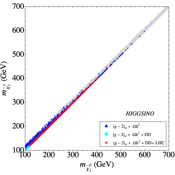
(b)

Figure 1: The results of our parameter scan in the $m_{\tilde{\chi}_{1}^{0}}$–$m_{\tilde{\chi}_{1}^{\pm}}$ plane for the higgsino DM scenario for current (left) and anticipated future limits (right) from $(g-2)_{\mu}$. For the color coding: see text.

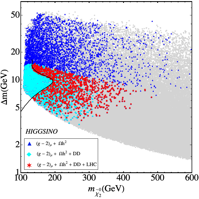
(a)

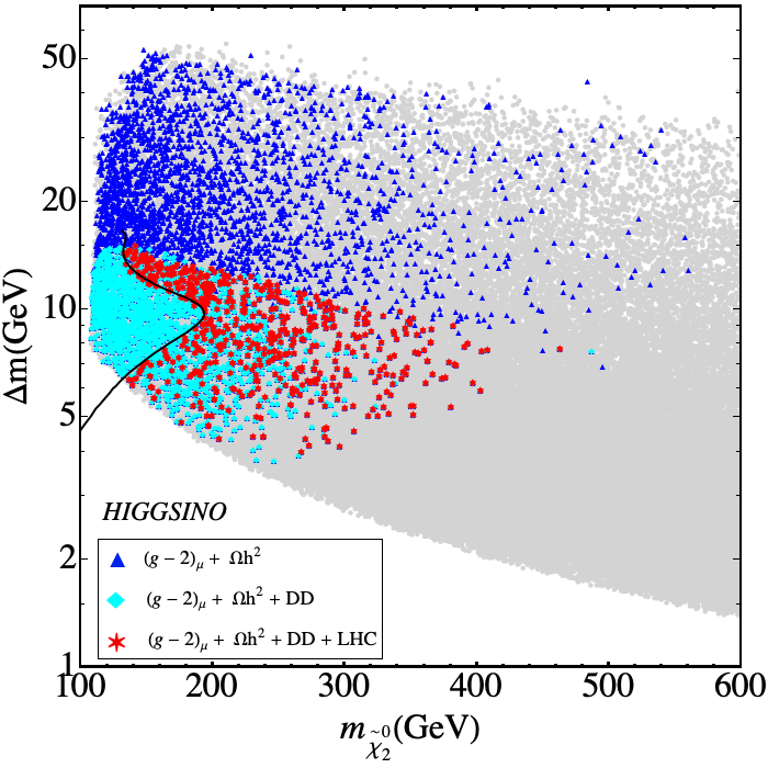
(b)

Figure 2: The results of our parameter scan in the $m_{\tilde{\chi}_{2}^{0}}$–$\Delta m(=m_{\tilde{\chi}_{2}^{0}}-m_{\tilde{\chi}_{1}^{0}})$ plane for the higgsino DM scenario for current (left) and anticipated future limits (right) from $(g-2)_{\mu}$. For the color coding: see text.

The impact of the DD experiments is demonstrated in Fig. 3. We show the $m_{\tilde{\chi}_{1}^{0}}$–$\sigma_{p}^{\rm SI}$ plane for current (left) and anticipated future limits (right) from $(g-2)_{\mu}$. The color coding of the points (from yellow to dark blue) denotes $M_{2}/\mu$, whereas in red we show the points fulfilling $(g-2)_{\mu}$ , relic density, DD and the LHC constraints. The black line indicates the current DD limits, here taken for sake of simplicity from XENON1T [8], as discussed in Sect. 3. It can be seen that a slight downward shift of this limit, e.g. due to additional DD experimental limits from LUX [6] or PANDAX [7], would not change our results in a strong way, but only slightly reduce the upper limit on $m_{\tilde{\chi}_{1}^{0}}$. The scanned parameter space extends from large $\sigma_{p}^{\rm SI}$ values, given for the smallest scanned $M_{2}/\mu$ values to the smallest ones, reached for the largest scanned $M_{2}/\mu$, i.e. the $\sigma_{p}^{\rm SI}$ constraints are particularly strong for small $M_{2}/\mu$, which can be understood as follows. The most important contribution to DM scattering comes from the exchange of a light ${{\cal CP}}$-even Higgs boson in the t-channel. The corresponding $h\tilde{\chi}_{1}^{0}\tilde{\chi}_{1}^{0}$ coupling at tree level is given by [108]

$$c_{h\tilde{\chi}_{1}^{0}\tilde{\chi}_{1}^{0}} \simeq -\frac{1}{2}(1+\sin 2\beta)\left(\tan^{2}\theta_{\mathrm{w}}\frac{M_{W}}{M_{1}-\mu}+\frac{M_{W}}{M_{2}-\mu}\right)\,,$$ (13)

where we have assumed $\mu>0$. Thus, the coupling becomes large for $\mu\sim M_{2}$ or $\mu\sim M_{1}$. Therefore, the XENON1T DD bound pushes the allowed parameter space into the almost pure higgsino-LSP region, with negligible bino and wino component. The impact of the compressed spectra searches is visible in the lower $m_{\tilde{\chi}_{1}^{0}}$ region. Given both CDM constraints and the LHC constraints, shown in red, the smallest $M_{2}/\mu$ value we find is 2.2 for both current and anticipated future $(g-2)_{\mu}$ bound. This result depends mildly on the assumed $(g-2)_{\mu}$ constraint, as this cuts away the largest $m_{\tilde{\chi}_{1}^{0}}$ values. All of the points will be conclusively probed by the future DD experiment XENONnT [109].

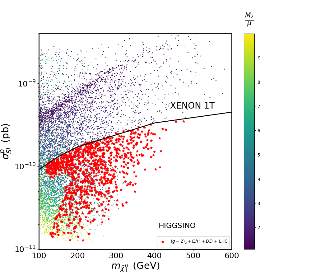
(a)

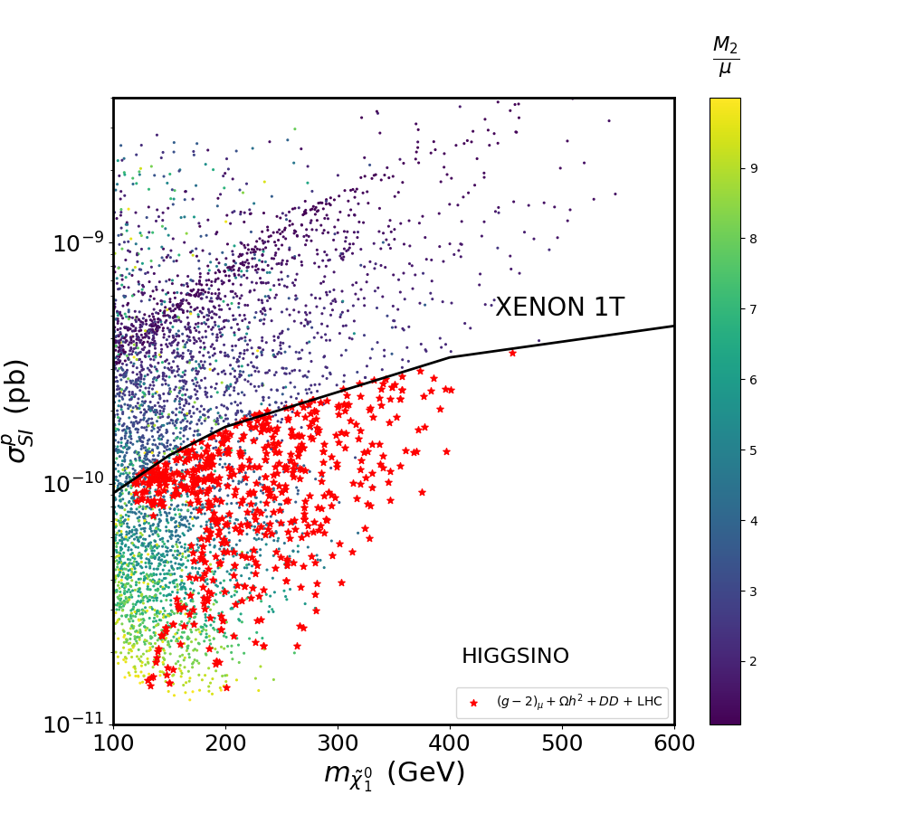
(b)

Figure 3: Scan results in the $m_{\tilde{\chi}_{1}^{0}}$–$\sigma_{p}^{\rm SI}$ plane for higgsino DM scenario for current (left) and anticipated future limits (right) from $(g-2)_{\mu}$. The color coding of the points denotes $M_{2}/\mu$ and the black line indicates the DD limits (see text). In red we show the points fulfilling the $(g-2)_{\mu}$ , relic density, DD and additionally the LHC constraints.

The distribution of $m_{\tilde{l}_{1}}$ (where it should be kept in mind that we have chosen the same masses for all three generations, see Sect. 2) is presented in the $m_{\tilde{\chi}_{1}^{0}}$–$m_{\tilde{l}_{1}}$ plane in Fig. 4, with the same color coding as in Fig. 1. The $(g-2)_{\mu}$ constraint places important constraints in this mass plane, since both types of masses enter into the contributing SUSY diagrams, see Sect. 3. The constraint is satisfied in a roughly triangular region with its tip around $(m_{\tilde{\chi}_{1}^{0}},m_{\tilde{l}_{1}})\sim(650\,\,\mathrm{GeV},700\,\,\mathrm{GeV})$ in the case of current $(g-2)_{\mu}$ constraints, and around $\sim(600\,\,\mathrm{GeV},600\,\,\mathrm{GeV})$ in the case of the anticipated future limits, i.e. the impact of the anticipated improved limits is clearly visible as an upper limit for both masses. Since no specific other requirement is placed on the slepton sector in the higgsino DM case the slepton masses are distributed over the $(g-2)_{\mu}$ allowed region. The DM relic density constraint, as discussed above, does not yield any further bounds on the allowed parameter space. The inclusion of the DM DD bounds, as visible by the cyan and red points, only cuts away the very largest slepton masses (for a given LSP mass).

The LHC constraints cut out all points with $m_{\tilde{\chi}_{1}^{0}}\;\raisebox{-3.00003pt}{$\stackrel{{\scriptstyle\displaystyle<}}{{\sim}}$}\;125\,\,\mathrm{GeV}$, as well as a triangular region with the tip around $(m_{\tilde{\chi}_{1}^{0}},m_{\tilde{l}_{1}})\sim(340\,\,\mathrm{GeV},450\,\,\mathrm{GeV})$. The first “cut” is due to the searches for compressed spectra. The second cut is mostly a result of the constraint coming from slepton pair production searches leading to dilepton and ${E\!\!\!\!/_{T}}$ in the final state [106]. The bound obtained by recasting the experimental search in CheckMATE is substantially weaker than the original limit from ATLAS. That limit is obtained for a ”simplified model” with $\text{BR}(\tilde{l}_{1},\tilde{l}_{2}\rightarrow l\tilde{\chi}_{1}^{0})=100\%$, an assumption which is not stritly valid in our parameter space. The small mass gap among $\tilde{\chi}_{1}^{0},\tilde{\chi}_{2}^{0}$ and $\tilde{\chi}_{1}^{\pm}$ allows significant BR of the sleptons to final states involving $\tilde{\chi}_{1}^{\pm}$ and $\tilde{\chi}_{2}^{0}$. This reduces the number of signal leptons and hence weakens the exclusion limit. Overall we can place an upper limit on the light slepton mass of about $\sim 1200\,\,\mathrm{GeV}$ and $1050\,\,\mathrm{GeV}$ for the current and the anticipated future accuracy of $(g-2)_{\mu}$, respectively. Since larger values of slepton masses are reached for lower values of $m_{\tilde{\chi}_{1}^{0}}$, the impact of $(g-2)_{\mu}$ is relatively weaker than in the case of chargino/neutralino masses.

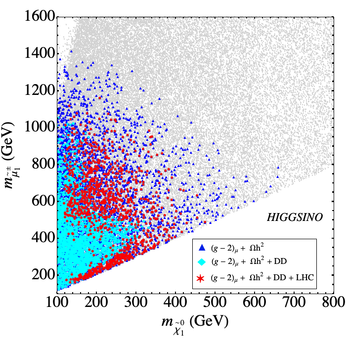
(a)

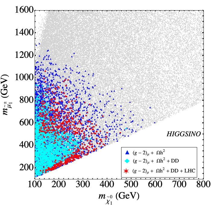
(b)

Figure 4: The results of our parameter scan in the $m_{\tilde{\chi}_{1}^{0}}$–$m_{\tilde{l}_{1}}$ plane for the higgsino DM scenario for current (left) and anticipated future limits (right) from $(g-2)_{\mu}$. The color coding is as in Fig. 1.

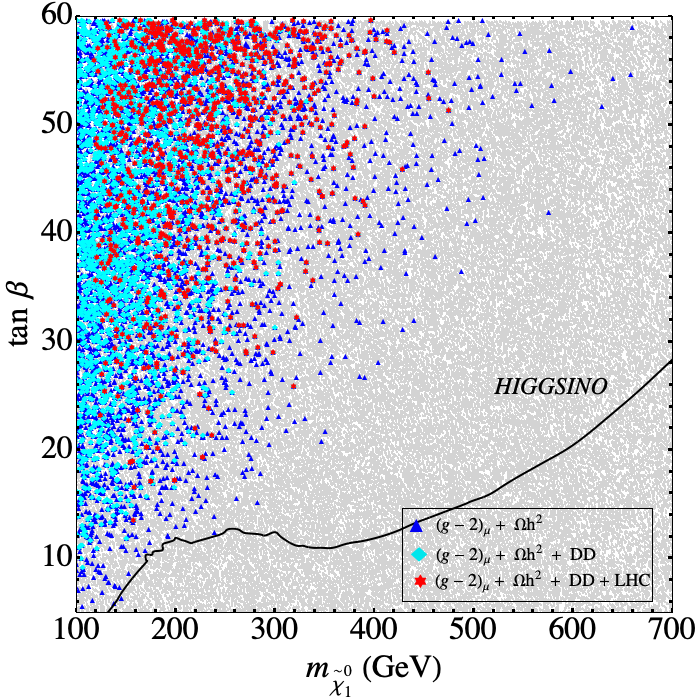
(a)

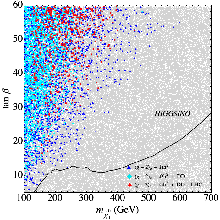
(b)

Figure 5: The results of our parameter scan in the $m_{\tilde{\chi}_{1}^{0}}$–$\tan\beta$ plane in the higgsino DM scenario for current (left) and anticipated future limits (right) from $(g-2)_{\mu}$. The color coding is as in Fig. 1. The black line indicates the current exclusion bounds for heavy MSSM Higgs bosons at the LHC (see text).

We finish our analysis of the higgsino DM case with the $m_{\tilde{\chi}_{1}^{0}}$–$\tan\beta$ plane presented in Fig. 5 with the same color coding as in Fig. 1. The $(g-2)_{\mu}$ constraint is fulfilled in a triangular region with the largest neutralino masses allowed for the largest $\tan\beta$ values (where we stopped our scan at $\tan\beta=60$), following the analytic dependence of the $(g-2)_{\mu}$ contributions in Sect. 3, $a_{\mu}\propto\tan\beta/m_{\rm EW}^{2}$ (where we denote with $m_{\rm EW}$ an overall EW mass scale. In agreement with the previous plots, the largest values for the lightest neutralino masses are $\sim 650\,\,\mathrm{GeV}$ $(\sim 600\,\,\mathrm{GeV})$ for the current (anticipated future) $(g-2)_{\mu}$ constraint. The DM relic density does not give any additional constraint. The points allowed by the DM DD limits (cyan and red) yield the observed reduction to about $\sim 500\,\,\mathrm{GeV}$. The LHC constraints cut out all points at low $m_{\tilde{\chi}_{1}^{0}}$, but nearly independent of $\tan\beta$. As observed before, they yield a small further reduction in the case of the anticipated future $(g-2)_{\mu}$ accuracy.

In Fig. 5 we also show as black lines the current bound from LHC searches for heavy neutral Higgs bosons [110] in the channel $pp\to H/A\to\tau\tau$ in the $M_{h}^{125}(\tilde{\chi})$ benchmark scenario (based on the search data published in Ref. [111] using $139\,\mbox{fb}^{-1}$.).  In this scenario light charginos and neutralinos are present, suppressing the $\tau\tau$ decay mode and thus yielding relatively weak limits in the $M_{A}$–$\tan\beta$ plane (see, e.g., Fig. 5 in [110]). The black lines correspond to $m_{\tilde{\chi}_{1}^{0}}=M_{A}/2$, i.e. roughly to the requirement for $A$-pole annihilation, where points above the black lines are experimentally excluded. It can be observed that all points allowed by $(g-2)_{\mu}$ are above the exclusion curve. This renders the effects of $A$-pole annihilation in this scenario effectively irrelevant (and justifies our choice to fix $M_{A}$ above the TeV scale).

5.2 Wino DM

The next case under investigation is the wino DM case, as discussed in Sect. 4.1. We follow the analysis flow as described in Sect. 4.2 and denote the points surviving certain constraints with different colors as defined in Sect. 5.1. The vacuum stability test had no effect on the points passing all other constraints.

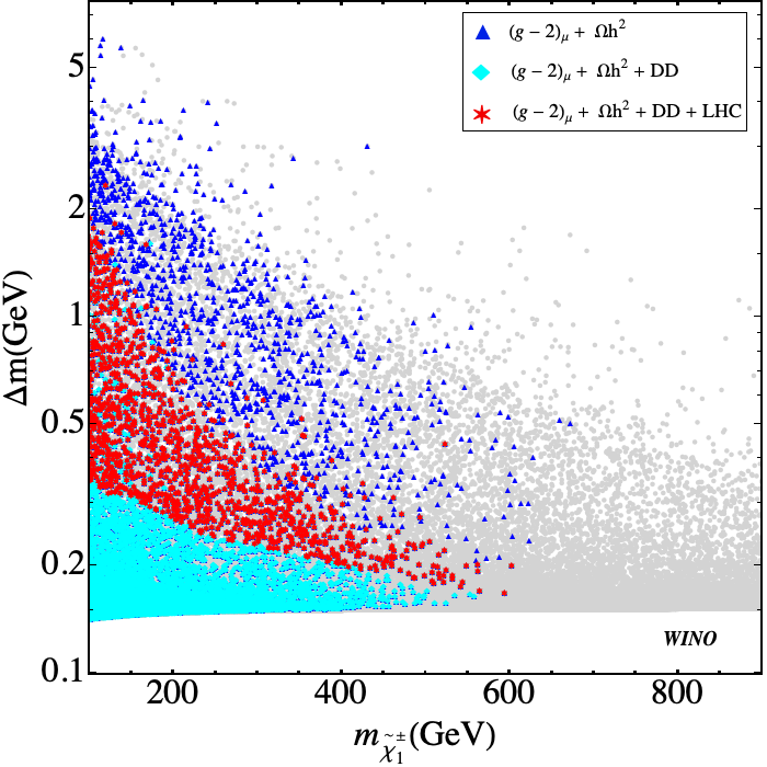
(a)

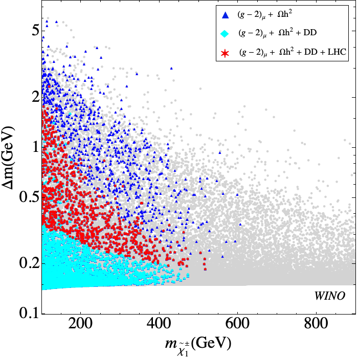
(b)

Figure 6: The results of our parameter scan in the $m_{\tilde{\chi}_{1}^{\pm}}-\Delta m(=m_{\tilde{\chi}_{1}^{\pm}}-m_{\tilde{\chi}_{1}^{0}})$ plane for the wino DM scenario for current (left) and anticipated future limits (right) from $(g-2)_{\mu}$. The color coding is as in Fig. 1.

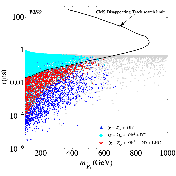
(a)

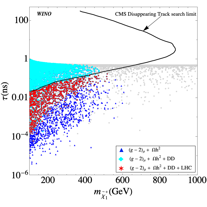
(b)

Figure 7: The results of our wino parameter scan in the $m_{\tilde{\chi}_{1}^{\pm}}$–$\tau$ plane for current (left) and anticipated future limits (right) from $(g-2)_{\mu}$, where $\tau$ is the lifetime of the chargino decaying to $\pi^{\pm}\tilde{\chi}_{1}^{0}$. The current limit from CMS [86] is shown as the black solid line. The color coding is as in Fig. 6.

In Fig. 6 we show our results in the $m_{\tilde{\chi}_{1}^{\pm}}$–$\Delta m(=m_{\tilde{\chi}_{1}^{\pm}}-m_{\tilde{\chi}_{1}^{0}})$ plane for the current (left) and future (right) $(g-2)_{\mu}$ constraint, see Eqs. (3) and (4), respectively. We display the results for $\Delta m$ rather than for $m_{\tilde{\chi}_{1}^{\pm}}$, since the mass difference is very small, and the various features are more easily visible in this plane. It should be remembered that we have applied the one-loop shift to, in particular, $m_{\tilde{\chi}_{1}^{0}}$ that allows for the decay $\tilde{\chi}_{1}^{\pm}\to\tilde{\chi}_{1}^{0}\pi^{\pm}$, see the discussion in Sect. 4.1. This results in the lower bound on $\Delta m$ of $\sim 0.15\,\,\mathrm{GeV}$. As in the higgsino scenario, see Sect. 5.1, all points that pass the $(g-2)_{\mu}$ constraint (current and anticipated future) also pass the relic density constraint, shown as blue triangles in Fig. 6. The highest allowed chargino masses are bounded from above by the $(g-2)_{\mu}$ constraint. The overall allowed parameter space, shown as red stars, is furthermore bounded from “above” by the DD limits and from “below” by the LHC constraints. The DD limits cut away larger mass differences, which can be understood as follows. The $h\tilde{\chi}_{1}^{0}\tilde{\chi}_{1}^{0}$ coupling for a wino-like $\tilde{\chi}_{1}^{0}$ is given by [108]

$$c_{h\tilde{\chi}_{1}^{0}\tilde{\chi}_{1}^{0}}\simeq\frac{M_{W}}{M_{2}^{2}-\mu^{2}}(M_{2}+\mu\sin 2\beta),$$ (14)

in the limit of $||\mu|-M_{2}|\gg M_{Z}$ and a decoupled ${{\cal CP}}$-odd Higgs boson (assuming also that the $h$-exchange dominates over the $H$ contribution in the (spin independent) DD bounds). This coupling becomes large for $\mu\sim M_{2}$. On the other hand, the tree level mass splitting between the wino-like states $\tilde{\chi}_{1}^{\pm}$ and $\tilde{\chi}_{1}^{0}$ generated (mainly by the mixing of the lighter chargino with the charged higgsino) is given as [117]

$$\Delta m(=m_{\tilde{\chi}_{1}^{\pm}}-m_{\tilde{\chi}_{1}^{0}})\simeq\frac{M_{W}^{4}(\sin 2\beta)^{2}\tan^{2}\theta_{\mathrm{w}}}{(M_{1}-M_{2})\mu^{2}},$$ (15)

for $|M_{1}-M_{2}|\gg M_{Z}$. The masss splitting increases for smaller $\mu$ values and thus coincides with larger DD cross sections, as discussed with Eq. (14). All limits together yield maximum $\Delta m\sim 2(0.2)\,\,\mathrm{GeV}$ for $m_{\tilde{\chi}_{1}^{\pm}}\sim 100(600)\,\,\mathrm{GeV}$ for the current $(g-2)_{\mu}$ constraint. The upper limit is reduced to $\sim 500\,\,\mathrm{GeV}$ for the future anticipated $(g-2)_{\mu}$ constraint.

The relevant LHC constraint is further analyzed in Fig. 7, where we show the plane $m_{\tilde{\chi}_{1}^{\pm}}$–$\tau_{\tilde{\chi}_{1}^{\pm}}$. $\tau_{\tilde{\chi}_{1}^{\pm}}$ denotes the lifetime of the chargino decaying to $\pi^{\pm}\tilde{\chi}_{1}^{0}$. Overlaid as black line is the bound from (CMS) charged disappearing track analysis [86]. One can observe that this constraint, cutting out parameter points between $\tau_{\tilde{\chi}_{1}^{\pm}}\sim 0.01$ ns and $\sim 1$ ns is responsible for the main LHC exclusion. It should be noted that in the “red star area” also some points appear cyan, i.e. excluded by (other) LHC searches, where the most relevant channels are pair production of sleptons leading to two leptons and ${E\!\!\!\!/_{T}}$ in the final state [106]. However, these channels are not strong enough to exclude more of the $m_{\tilde{\chi}_{1}^{\pm}}$–$\tau_{\tilde{\chi}_{1}^{\pm}}$ plane than the disappearing track search. It can be expected in the (near) future that improved DD bounds, cutting the allowed parameter space from small $\tilde{\chi}_{1}^{\pm}$ lifetime and improved disappearing track searches, cutting from large lifetimes, may substantially shrink the allowed parameter space, sharpening the upper limit on $m_{\tilde{\chi}_{1}^{\pm}}$ and the prospects for future collider searches. The two bounds together have the potential to firmly rule out the case of wino DM in the MSSM, will be discussed below.

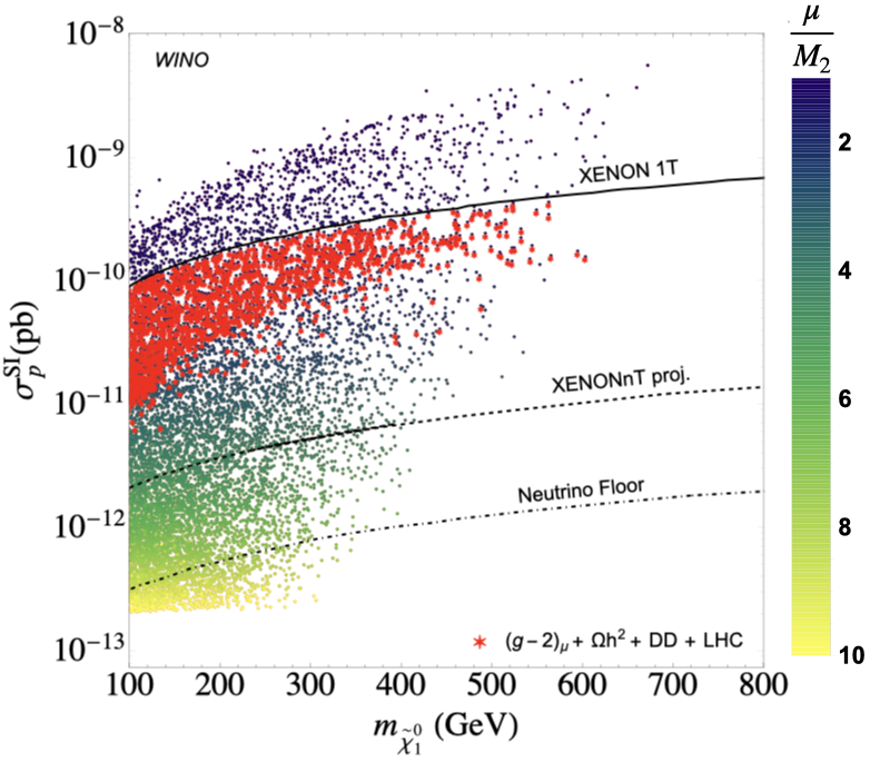
(a)

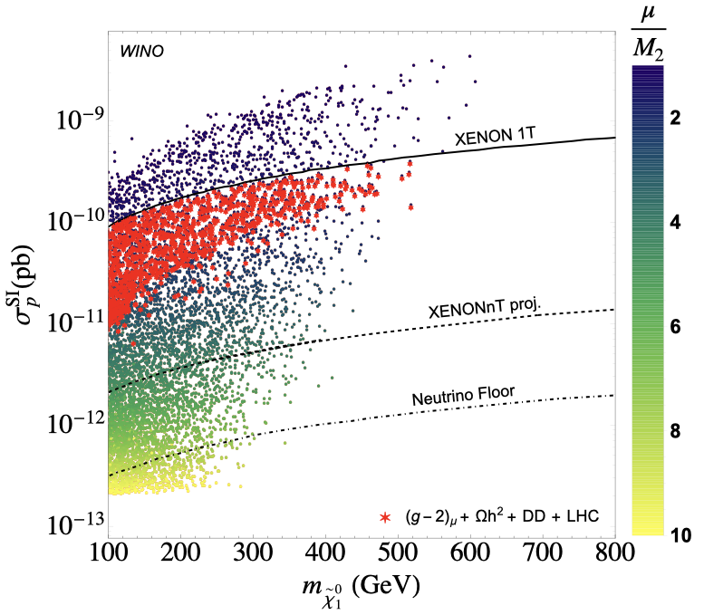
(b)

Figure 8: Scan results in the $m_{\tilde{\chi}_{1}^{0}}$-$\sigma_{p}^{\rm SI}$ plane for the wino DM scenario for current (left) and anticipated future limits (right) from $(g-2)_{\mu}$. The color coding of the points denotes $\mu/M_{2}$ and the black solid line indicates the current DD limit from XENON-1T while the black dashed and dot-dashed lines are respectively the projected reach of XENON-nT and coherent neutrino scattering floor. In red we show the points fulfilling $(g-2)_{\mu}$ , relic density, DD and additionally the LHC constraints.

The impact of the DD experiments is demonstrated in Fig. 8. We show the $m_{\tilde{\chi}_{1}^{0}}$–$\sigma_{p}^{\rm SI}$ plane for current (left) and anticipated future limits (right) from $(g-2)_{\mu}$. The color coding of the points (from yellow to dark green) denotes $\mu/M_{2}$, whereas in red we show the points fulfilling $(g-2)_{\mu}$ , relic density, DD and the LHC constraints. The solid black line indicates the current DD limits, here taken for sake of simplicity from XENON1T [8], as discussed in Sect. 3. It can be seen that a slight downward shift of this limit, e.g. due to additional DD experimental limits from LUX [6] or PANDAX [7], would not change our results in a relevant way. However, moderately improved limits may have a strong impact, as discussed above. The scanned parameter space extends from large $\sigma_{p}^{\rm SI}$ values, given for the smallest scanned $\mu/M_{2}$ values to the smallest ones, reached for the largest scanned $\mu/M_{2}$, i.e. the $\sigma_{p}^{\rm SI}$ constraints are particularly strong for small $\mu/M_{2}$. Given both CDM constraints and the LHC constraints, shown in red, the smallest $\mu/M_{2}$ value we find is 1.5 for both the current and anticipated future $(g-2)_{\mu}$ bound. As mentioned above, the DD bound can become relevantly stronger with future experiments. We show as dashed line the projected limit of XENONnT [109], and the dot-dashed line indicates the neutrino floor [118]. One can see that the XENONnT result will either firmly exlude or detect a wino DM candidate, possibly in conjunction with improved disappearing track searches at the LHC, as discussed above.

The distribution of the lighter slepton mass (where it should be kept in mind that we have chosen the same masses for all three generations, see Sect. 2) is presented in the $m_{\tilde{\chi}_{1}^{0}}$–$m_{\tilde{l}_{1}}$ plane in Fig. 9, with the same color coding as in Fig. 6. The $(g-2)_{\mu}$ constraint places important constraints in this mass plane, since both types of masses enter into the contributing SUSY diagrams, see Sect. 3 (and obviously all points pass the DM relic density upper limit). The $(g-2)_{\mu}$ constraint is satisfied in a triangular region with its tip around $(m_{\tilde{\chi}_{1}^{0}},m_{\tilde{l}_{1}})\sim(700\,\,\mathrm{GeV},700\,\,\mathrm{GeV})$ in the case of current $(g-2)_{\mu}$ constraints, and around $\sim(600\,\,\mathrm{GeV},700\,\,\mathrm{GeV})$ in the case of the anticipated future limits. The highest slepton masses reached are about $1500(1200)\,\,\mathrm{GeV}$, respectively; i.e. the impact of the anticipated improved limits is clearly visible as an upper limit. After including the DD and LHC constraints the upper limits for the LSP are slightly reduced by $\sim 100\,\,\mathrm{GeV}$, whereas the upper limits on sleptons are not affected. Concerning the LHC searches, the constraints from slepton pair production searches rule out some parameter points from the low $m_{\tilde{l}_{1}}$ region. Larger slepton masses are excluded by the same search if the “second” slepton turns out to be relatively light. Points excluded by compressed spectra searches [84], depending on the lightest chargino mass, can be found all over the plane.

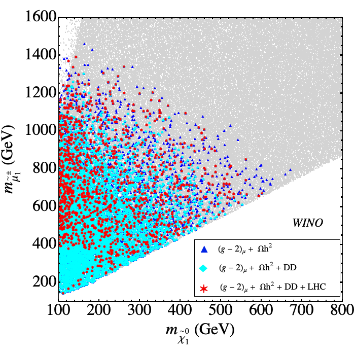
(a)

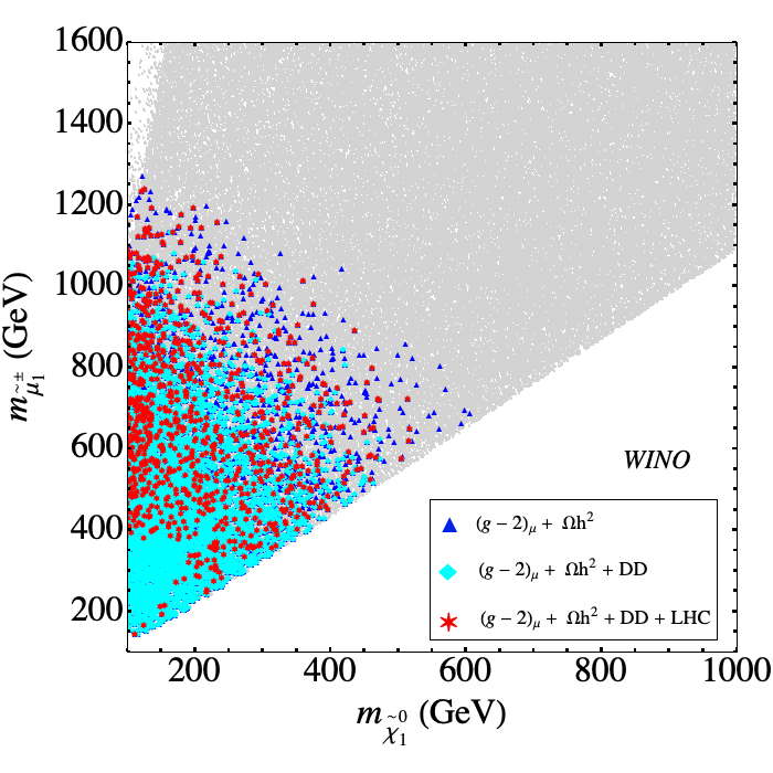
(b)

Figure 9: The results of our parameter scan in the $m_{\tilde{\chi}_{1}^{0}}$–$m_{\tilde{\mu}_{1}}$ plane for the wino DM scenario for current (left) and anticipated future limits (right) from $(g-2)_{\mu}$. The color coding is as in Fig. 6.

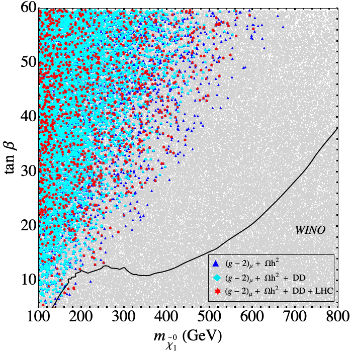
(a)

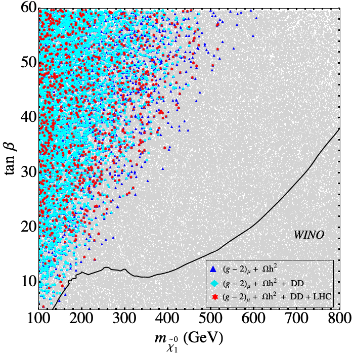
(b)

Figure 10: The results of our parameter scan in the $m_{\tilde{\chi}_{1}^{0}}$-$\tan\beta$ plane in the wino DM scenario for current (left) and anticipated future limits (right) from $(g-2)_{\mu}$. The color coding is as in Fig. 6. The black line indicates the current exclusion bounds for heavy MSSM Higgs bosons at the LHC (see text).

We finish our analysis of the wino DM case with the $m_{\tilde{\chi}_{1}^{0}}$-$\tan\beta$ plane presented in Fig. 10 with the same color coding as in Fig. 6. The $(g-2)_{\mu}$ constraint is fulfilled in a triangular region with largest neutralino masses allowed for the largest $\tan\beta$ values (where we stopped our scan at $\tan\beta=60$), following the analytic dependence of the $(g-2)_{\mu}$ contributions in Sect. 3, $a_{\mu}\propto\tan\beta/m_{\rm EW}^{2}$ (where we denote with $m_{\rm EW}$ an overall EW mass scale. In agreement with the previous plots, the largest values for the lightest neutralino masses are $\sim 600\,\,\mathrm{GeV}$ $(\sim 500\,\,\mathrm{GeV})$ for the current (anticipated future) $(g-2)_{\mu}$ constraint. The points allowed by the DM constraints (blue/cyan) are distributed all over the allowed region. The LHC constraints also cut out points distributed all over the allowed triangle, in agreement with the previous discussion.

In Fig. 10 we also show as black lines the current bound from LHC searches for heavy neutral Higgs bosons [111, 110], see the discussion in Sect. 5.1. Points above the black lines are experimentally excluded. There are a few points passing the current $(g-2)_{\mu}$ constraint below the black $A$-pole line, reaching up to $m_{\tilde{\chi}_{1}^{0}}\sim 220\,\,\mathrm{GeV}$, for which the $A$-pole annihilation could provide the correct DM relic density. For the anticipated future accuracy in $(g-2)_{\mu}$ this mechanism would effectively be absent, making the $A$-pole annihilation in this scenario marginal.

5.3 Bino/wino and bino DM

In this section we analyze the case of bino/wino and bino DM, as defined in Sect. 4.1. The three cases defined there correspond exactly to the set of analyses in Ref. [15]. However, we now apply the DM relic density as an upper bound (“DM upper bound”), whereas in Ref. [15] the LSP was required to give the full amount of CDM (“DM full”). Since overall the results are similar to the ones found in Ref. [15], we will keep the discussion brief, but try to highlight the differences w.r.t. Ref. [15]. For all scenarios we find that the vacuum stability bounds have no impact on the final mass limits found.

5.3.1 Bino/wino DM with $\tilde{\chi}_{1}^{\pm}$-coannihilation

In Fig. 11 we show our results in the $m_{\tilde{\chi}_{1}^{0}}$–$m_{\tilde{\chi}_{1}^{\pm}}$ plane for the current (left) and future (right) $(g-2)_{\mu}$ constraint, see Eqs. (3) and (4), respectively. The color coding is defined in Sect. 5.1. By definition of $\tilde{\chi}_{1}^{\pm}$-coannihilation the points are clustered in the diagonal of the plane. Overall we observe here exactly the same pattern of points as in the case of “DM full” [15]. After taking into account all constraints we find upper limits of $\sim 600(500)\,\,\mathrm{GeV}$ in the case of the current (future) $(g-2)_{\mu}$ limits. Thus, the experimental data set about the same upper as well as lower bounds as in Ref. [15] (modulo differences due to point density artefacts). Consequently, the search targets for the upcoming LHC runs particular for future $e^{+}e^{-}$ colliders remain about the same.

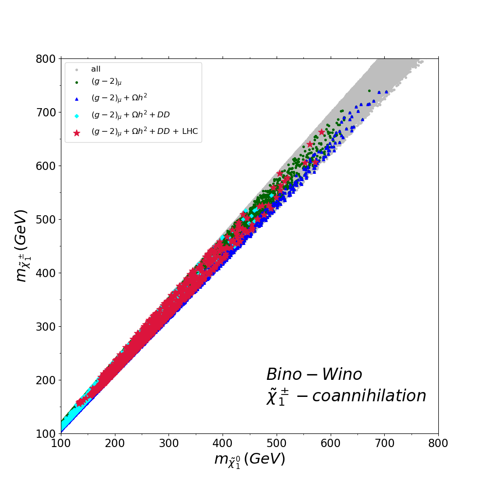
(a)

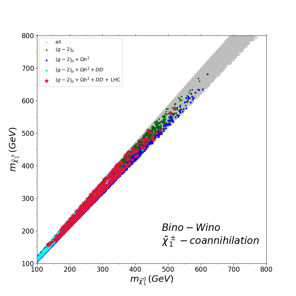
(b)

Figure 11: The results of our parameter scan in the $m_{\tilde{\chi}_{1}^{0}}-m_{\tilde{\chi}_{1}^{\pm}}$ plane for the bino-wino $\tilde{\chi}_{1}^{\pm}$-coannihilation scenario for current (left) and anticipated future limits (right) from $(g-2)_{\mu}$. For the color coding: see text.

The impact of the DD experiments is demonstrated in Fig. 12. We show the $m_{\tilde{\chi}_{1}^{0}}$–$\sigma_{p}^{\rm SI}$ plane for current (left) and anticipated future limits (right) from $(g-2)_{\mu}$. The color coding of the points (from yellow to dark green) denotes $\mu/M_{1}$, whereas in red we show the points fulfilling all constraints including the LHC ones. As in Fig. 3 the solid black line indicates the current DD limits from XENON1T [8]. Also here the results are in very good agreement with Ref. [15] (again modulo point density artefacts). The scanned parameter space extends from large $\sigma_{p}^{\rm SI}$ values, given for the smallest scanned $\mu/M_{1}$ values to the smallest ones, reached for the largest scanned $\mu/M_{1}$, i.e. the $\sigma_{p}^{\rm SI}$ constraints are particularly strong for small $\mu/M_{1}$. Given in red the points fulfilling $(g-2)_{\mu}$ , both CDM constraints and the LHC constraints, the smallest $\mu/M_{1}$ value we find is 1.67 for the current and 1.78 for the anticipated future $(g-2)_{\mu}$ bound. The dashed line indicates the projected XENONnT limit [109], and the dot-dashed line indicates the neutrino floor [118]. One can see that XENONnT will not be able to fully test the chargino co-annihilation scenario, with some points that pass all constraints (red) being even below the neutrino floor.

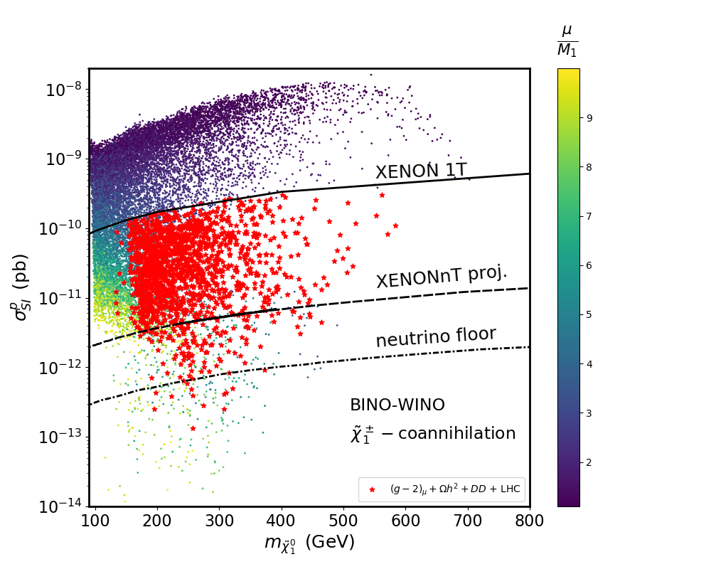
(a)

(b)

Figure 12: Scan results in the $m_{\tilde{\chi}_{1}^{0}}$–$\sigma_{p}^{\rm SI}$ plane for bino-wino $\tilde{\chi}_{1}^{\pm}$-coannihilation scenario for current (left) and anticipated future limits (right) from $(g-2)_{\mu}$. The color coding of the points denotes $\mu/M_{1}$ and the black lines indicates the DD limits (see text). In red we show the points fulfilling $(g-2)_{\mu}$ , the relic density, DD and the LHC constraints.

The distribution of the lighter slepton mass (where it should be kept in mind that we have chosen the same masses for all three generations, see Sect. 2) is presented in the $m_{\tilde{\chi}_{1}^{0}}$–$m_{\tilde{l}_{1}}$ plane in Fig. 13, with the same color coding as in Fig. 11. The $(g-2)_{\mu}$ constraint places important constraints in this mass plane, since both types of masses enter into the contributing SUSY diagrams, see Sect. 3. The constraint is satisfied in a triangular region with its tip around $(m_{\tilde{\chi}_{1}^{0}},m_{\tilde{l}_{1}})\sim(700\,\,\mathrm{GeV},800\,\,\mathrm{GeV})$ in the case of current $(g-2)_{\mu}$ constraints, and around $\sim(600\,\,\mathrm{GeV},700\,\,\mathrm{GeV})$ in the case of the anticipated future limits, i.e. the impact of the anticipated improved limits is clearly visible as an upper limit. These results remain unchanged w.r.t. the “DM full” case [15]. The points fulfilling the DM relic density constraint (blue/cyan/red) are distributed all over the $(g-2)_{\mu}$ allowed range. They extend to somewhat higher slepton masses as compared to Ref. [15], due to the less restrictive DM upper bound. The DD limits cut away the largest values, in particular for $m_{\tilde{l}_{1}}$, which can be understood as follows. Large $m_{\tilde{l}_{1}}$ values, with correspondingly large sneutrino masses, require smaller $\mu$ to satisfy the $(g-2)_{\mu}$ constraint. This in turn puts them in tension with the DD bounds, see Fig. 12.

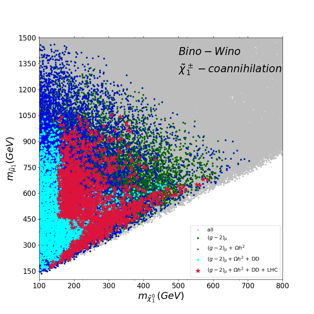
(a)

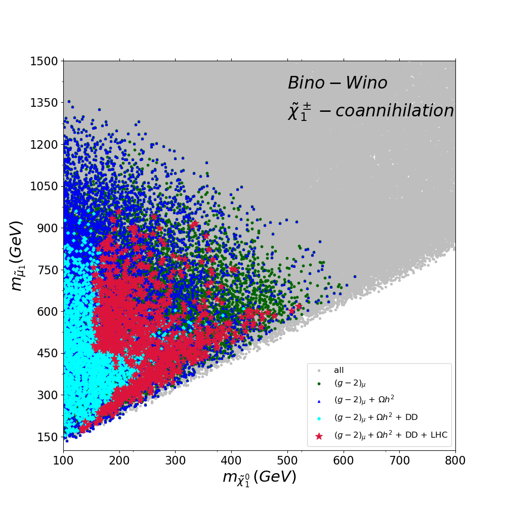
(b)

Figure 13: The results of our parameter scan in the $m_{\tilde{\chi}_{1}^{0}}$–$m_{\tilde{l}_{1}}$ plane for the bino-wino $\tilde{\chi}_{1}^{\pm}$-coannihilation scenario for current (left) and anticipated future limits (right) from $(g-2)_{\mu}$. The color coding is as in Fig. 11.

The LHC constraints cut out lower slepton masses, following the same pattern as in Ref. [15]. They cut away masses up to $m_{\tilde{l}_{1}}\;\raisebox{-3.00003pt}{$\stackrel{{\scriptstyle\displaystyle<}}{{\sim}}$}\;450\,\,\mathrm{GeV}$, as well as part of the very low $m_{\tilde{\chi}_{1}^{0}}$ points nearly independent of $m_{\tilde{l}_{1}}$. Here the latter “cut” is due to the searches for compressed spectra with $\tilde{\chi}_{1}^{\pm},\tilde{\chi}_{2}^{0}$ decaying via off-shell gauge bosons [84]. The first “cut” is mostly a result of the searches for slepton pair production with a decay to two leptons plus missing energy [106]. As was demonstrated and discussed in detail in Ref. [15] for this limit it is crucial to employ a proper re-cast of the LHC searches, rather than a naive application of the published bounds, Overall we can place an upper limit on the light slepton mass of about $\sim 1050\,\,\mathrm{GeV}$ and $\sim 950\,\,\mathrm{GeV}$ for the current and the anticipated future accuracy of $(g-2)_{\mu}$, respectively.

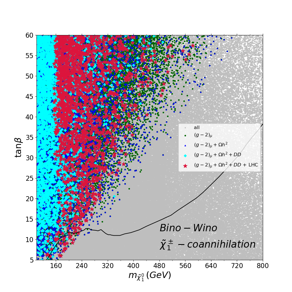
(a)

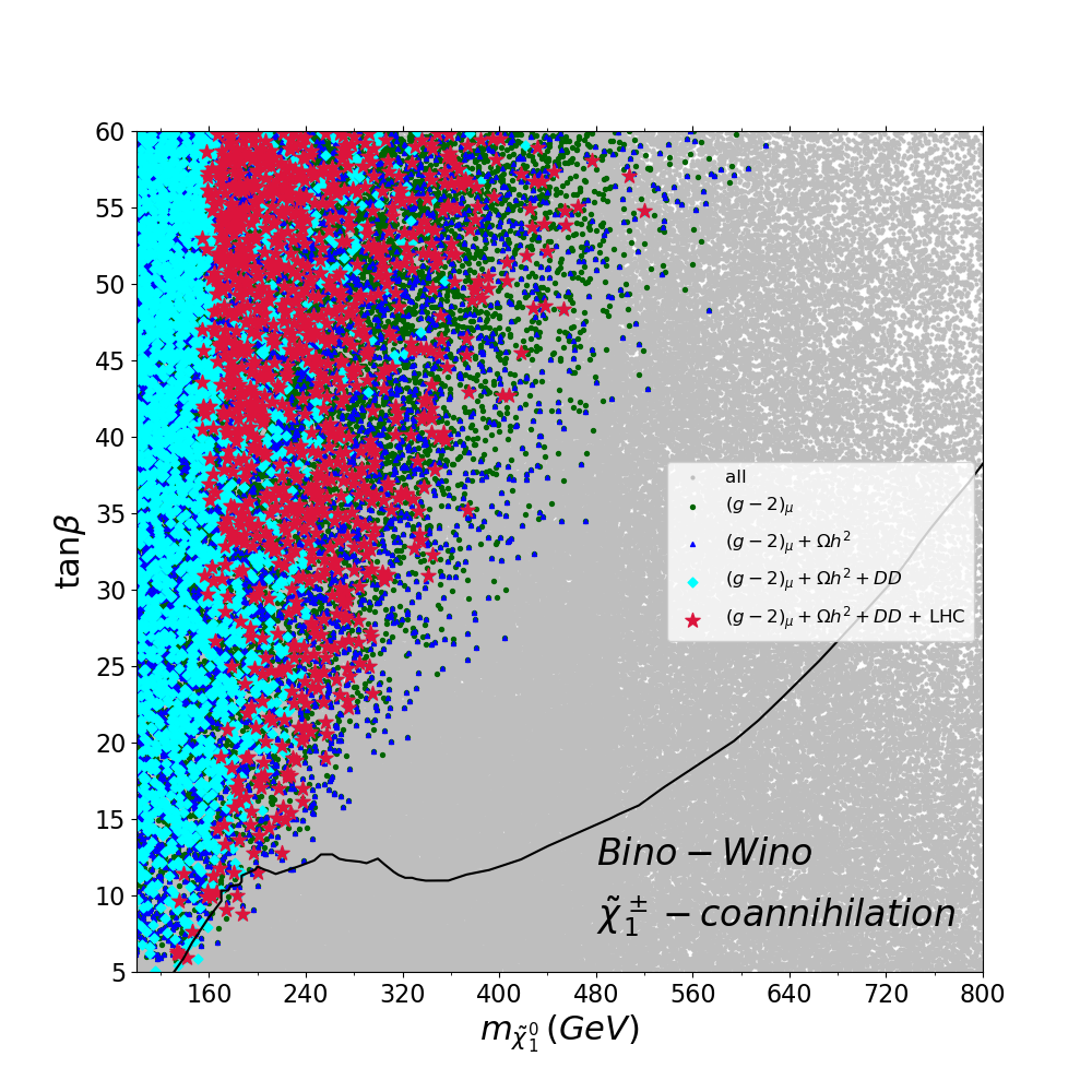
(b)

Figure 14: The results of our parameter scan in the $m_{\tilde{\chi}_{1}^{0}}$–$\tan\beta$ plane in the bino-wino $\tilde{\chi}_{1}^{\pm}$-coannihilation scenario for current (left) and anticipated future limits (right) from $(g-2)_{\mu}$. The color coding is as in Fig. 11. The black line indicates the current exclusion bounds for heavy MSSM Higgs bosons at the LHC (see text).

We finish our analysis of the $\tilde{\chi}_{1}^{\pm}$-coannihilation case with the $m_{\tilde{\chi}_{1}^{0}}$–$\tan\beta$ plane presented in Fig. 14 with the same color coding as in Fig. 11. For this plane we find that the results are in full agreement with the “DM full” case as analyzed in Ref. [15]. The $(g-2)_{\mu}$ constraint is fulfilled in a triangular region with largest neutralino masses allowed for the largest $\tan\beta$ values ($\tan\beta=60$). In agreement with the previous plots, the largest values for the lightest neutralino masses are $\sim 600\,\,\mathrm{GeV}$ $(\sim 500\,\,\mathrm{GeV})$ for the current (anticipated future) $(g-2)_{\mu}$ constraint. The points allowed by the DM constraints (blue/cyan) are distributed all over the allowed region. The LHC constraints cut out points at low $m_{\tilde{\chi}_{1}^{0}}$, but nearly independent on $\tan\beta$.

As in the previous scenarios, in Fig. 14 we also show as black lines the current bound from LHC searches for heavy neutral Higgs bosons [110] in the channel $pp\to H/A\to\tau\tau$ in the $M_{h}^{125}(\tilde{\chi})$ benchmark scenario. As before the black lines correspond to $m_{\tilde{\chi}_{1}^{0}}=M_{A}/2$, i.e. roughly to the requirement for $A$-pole annihilation, where points above the black lines are experimentally excluded. The improved limits of the experimental analysis based on $139\mbox{fb}^{-1}$ [111], but now with the relaxed DM relic density bound, still allow parameter points that cannot be regarded as excluded. They are found for $m_{\tilde{\chi}_{1}^{0}}\;\raisebox{-3.00003pt}{$\stackrel{{\scriptstyle\displaystyle<}}{{\sim}}$}\;240(200)\,\,\mathrm{GeV}$ and $\tan\beta\;\raisebox{-3.00003pt}{$\stackrel{{\scriptstyle\displaystyle<}}{{\sim}}$}\;12$ in the case of the current (anticipated future) $(g-2)_{\mu}$ constraints. To analyze these points a dedicated analysis of the $A$-pole annihilation would be required. This dedicated analysis we leave for future work.

5.3.2 Bino DM with $\tilde{l}^{\pm}$-coannihilation case-L

We now turn to the case of bino DM with $\tilde{l}^{\pm}$-coannihilation. As discussed in in Sect. 4.1 we distinguish two cases, depending which of the two slepton soft SUSY-breaking parameters is set to be close to $m_{\tilde{\chi}_{1}^{0}}$. We start with the Case-L, where we chose $m_{\tilde{l}_{L}}\sim M_{1}$, i.e. the left-handed charged sleptons as well as the sneutrinos are close in mass to the LSP. We find that all six sleptons are close in mass and differ by less than $\sim 50\,\,\mathrm{GeV}$.

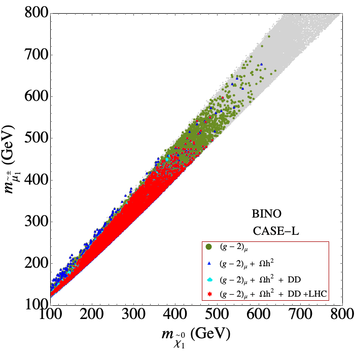
(a)

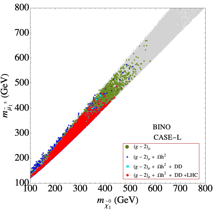
(b)

Figure 15: The results of our parameter scan in the $m_{\tilde{\chi}_{1}^{0}}$–$m_{\tilde{\mu}_{1}}$ plane for the $\tilde{l}$-coannihilation case-L scenario for current (left) and anticipated future limits (right) from $(g-2)_{\mu}$. The color coding is as in Fig. 6.

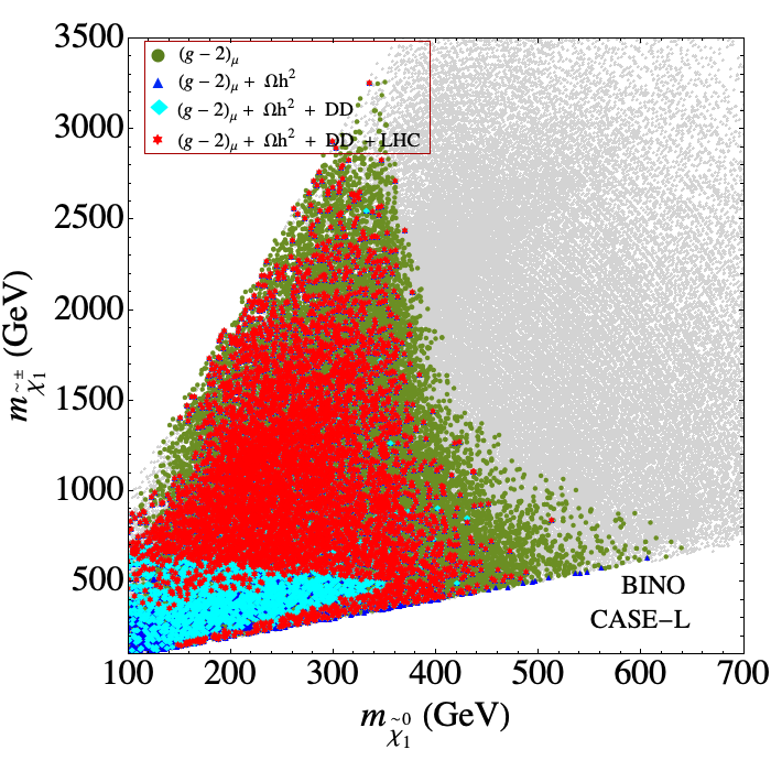
(a)

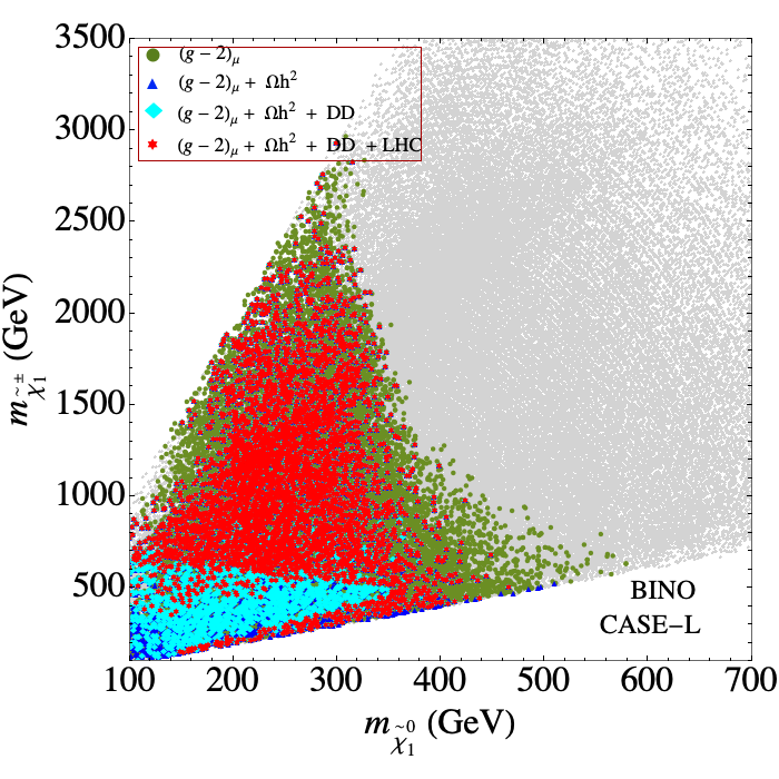
(b)

Figure 16: The results of our parameter scan in the $m_{\tilde{\chi}_{1}^{0}}-m_{\tilde{\chi}_{1}^{\pm}}$ plane for the $\tilde{l}$-coannihilation case-L scenario for current (left) and anticipated future limits (right) from $(g-2)_{\mu}$. The color coding is as in Fig. 15.

In Fig. 15 we show the results of our scan in the $m_{\tilde{\chi}_{1}^{0}}$–$m_{\tilde{\mu}_{1}}$ plane, as before for the current $(g-2)_{\mu}$ constraint (left) and the anticipated future constraint (right). The color coding of the points is the same as in Fig. 1, see the description in the beginning of Sect. 5.1. By definition of the scenario, the points are located along the diagonal of the plane. The result is qualitatively similar to the analysis in Ref. [15], where the relic density constraint was used as a direct measurement, and not only as an upper limit. However, one can observe that a slightly larger mass difference between the $\tilde{\mu}_{1}$ and the $\tilde{\chi}_{1}^{0}$ is allowed in comparison with Ref. [15]. Taking all bounds into account we find upper limits on the LSP mass of $\sim 500\,\,\mathrm{GeV}$ and $\sim 450\,\,\mathrm{GeV}$ for the current and anticipated future $(g-2)_{\mu}$ accuracy, respectively. The limits on $m_{\tilde{\mu}_{1}}$ are about $\sim 50-100\,\,\mathrm{GeV}$ larger.

In Fig. 16 we show the results in the $m_{\tilde{\chi}_{1}^{0}}$–$m_{\tilde{\chi}_{1}^{\pm}}$ plane with the same color coding as in Fig. 15. The results are again qualitatively in agreement with Ref. [15]. However, in particular for the future $(g-2)_{\mu}$ constraint, slightly larger values of $m_{\tilde{\chi}_{1}^{\pm}}$ are allowed. Overall we find for the light charginos mass an upper limit of $\sim 3200\,\,\mathrm{GeV}$ ($\sim 2900\,\,\mathrm{GeV}$) for the current (anticipated future $(g-2)_{\mu}$ ) constraint. Clearly visible are the LHC constraints for $\tilde{\chi}_{2}^{0}$–$\tilde{\chi}_{1}^{\pm}$ pair production leading to three leptons and ${E\!\!\!\!/_{T}}$ in the final state [119]. At very low values of both $m_{\tilde{\chi}_{1}^{0}}$ and $m_{\tilde{\chi}_{1}^{\pm}}$ the compressed specta searches [84] cut away points up to $m_{\tilde{\chi}_{1}^{0}}\;\raisebox{-3.00003pt}{$\stackrel{{\scriptstyle\displaystyle<}}{{\sim}}$}\;150\,\,\mathrm{GeV}$.

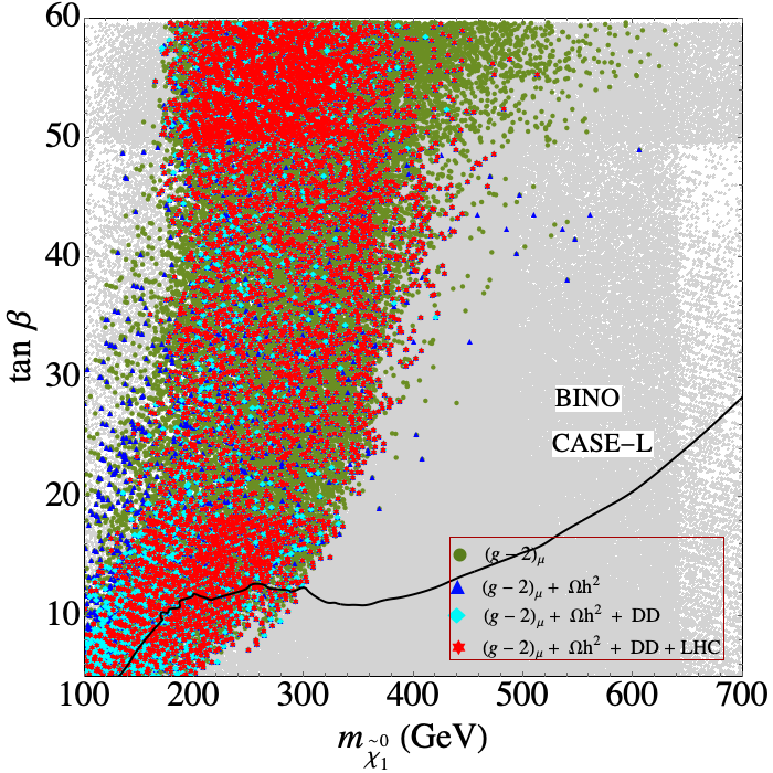
(a)

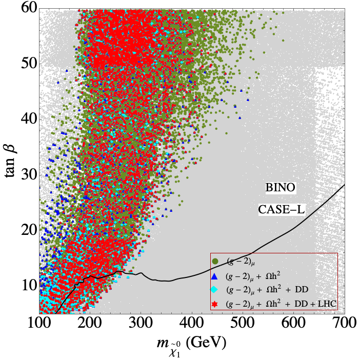
(b)

Figure 17: The results of our parameter scan in the $m_{\tilde{\chi}_{1}^{0}}$–$\tan\beta$ plane in the $\tilde{l}$-coannihilation case-L scenario for current (left) and anticipated future limits (right) from $(g-2)_{\mu}$. The color coding is as in Fig. 15. The black line indicates the current exclusion bounds for heavy MSSM Higgs bosons at the LHC (see text).

The results for the $\tilde{l}^{\pm}$-coannihilation Case-L in the $m_{\tilde{\chi}_{1}^{0}}$–$\tan\beta$ plane are presented in Fig. 17.  The overall picture is similar to the $\tilde{\chi}_{1}^{\pm}$-coannhiliation case shown above in Fig. 14. As above they are also qualitatively and quantitatively similar to the results of Case-L with the relic density taken as a direct measurement as presented in Ref. [15]. Larger LSP masses are allowed for larger $\tan\beta$ values. On the other hand the combination of small $m_{\tilde{\chi}_{1}^{0}}$ and large $\tan\beta$ leads to a too large contribution to $a_{\mu}^{\rm SUSY}$ and is thus excluded. As in the other scenarios we also show the limits from $H/A$ searches at the LHC as a solid line. In this case for the current and anticipated future $(g-2)_{\mu}$ limit substantially more points passing the $(g-2)_{\mu}$ constraint “survive” below the black line(s), i.e. they are potential candidates for $A$-pole annihilation. The masses reach up to $\sim 300\,\,\mathrm{GeV}$ and $\sim 250\,\,\mathrm{GeV}$, respectively. These limits are slightly higher compared to the case with the relic density measurement taken as a direct measurement [15].

5.3.3 Bino DM with $\tilde{l}^{\pm}$-coannihilation case-R

We now turn to our fifth scenario, bino DM with $\tilde{l}^{\pm}$-coannihilation Case-R, where in the scan we require the “right-handed” sleptons to be close in mass with the LSP. It should be kept in mind that in our notation we do not mass-order the sleptons: for negligible mixing as it is given for selectrons and smuons the “left-handed” (“right-handed”) slepton corresponds to $\tilde{l}_{1}$ ($\tilde{l}_{2}$). As it will be seen below, in this scenario all relevant mass scales are required to be relatively light by the $(g-2)_{\mu}$ constraint.

We start in Fig. 18 with the $m_{\tilde{\chi}_{1}^{0}}$–$m_{\tilde{\mu}_{2}}$ plane with the same color coding as in Fig. 11. By definition of the scenario the points are concentrated on the diagonal. The current (future) $(g-2)_{\mu}$ bound yields upper limits on the LSP of $\sim 700(600)\,\,\mathrm{GeV}$, as well as an upper limit on $m_{\tilde{\mu}_{2}}$ (which is close in mass to the $\tilde{e}_{2}$ and ${\tilde{\tau}_{2}}$) of $\sim 800(700)\,\,\mathrm{GeV}$. These limits remain unchanged by the inclusion of the DM relic density bound. The limits agrees well with the ones found in the case with the relic density measurement taken as a direct measurement [15]. Including the DD and LHC constraints, these limits reduce to $\sim 500\leavevmode\nobreak\ (380)\,\,\mathrm{GeV}$ for the LSP for the current (future) $(g-2)_{\mu}$ bounds, and correspondingly to $\sim 550\leavevmode\nobreak\ (440)\,\,\mathrm{GeV}$ for $m_{\tilde{\mu}_{2}}$. The LHC constraints cut out some, but not all lower-mass points, where the searches for compressed slepton/neutralino spectra [84] are most relevant. Due to the larger splitting the “right-handed” stau turns out to be the NLSP in this scenario, where the uppoer bounds are found at $\sim 500\leavevmode\nobreak\ (380)\,\,\mathrm{GeV}$ for the current (anticipated future) $(g-2)_{\mu}$ bounds.

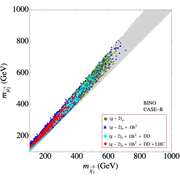
(a)

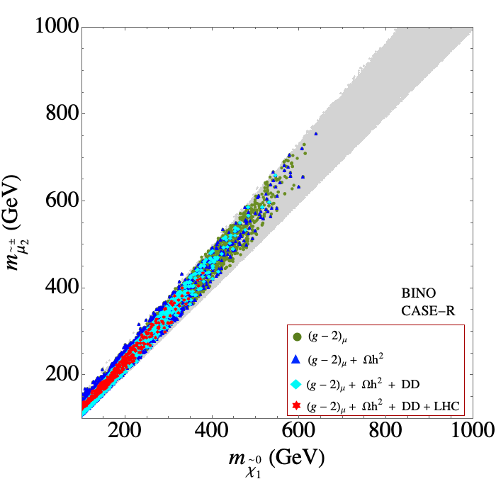
(b)

Figure 18: The results of our parameter scan in the $m_{\tilde{\chi}_{1}^{0}}$–$m_{\tilde{\mu}_{2}}$ plane for the $\tilde{l}$-coannihilation case-R scenario for current (left) and anticipated future limits (right) from $(g-2)_{\mu}$. The color coding is as in Fig. 15.

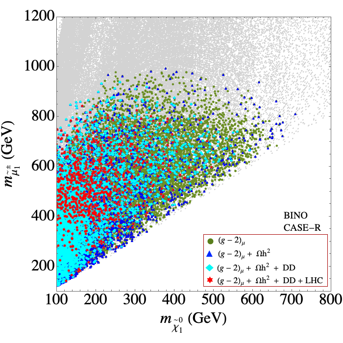
(a)

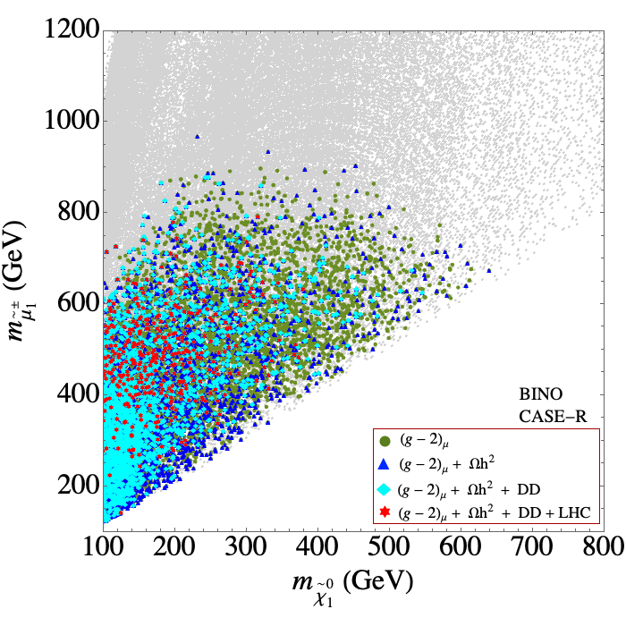
(b)

Figure 19: The results of our parameter scan in the $m_{\tilde{\chi}_{1}^{0}}$–$m_{\tilde{\mu}_{1}}$ plane for the $\tilde{l}$-coannihilation case-R scenario for current (left) and anticipated future limits (right) from $(g-2)_{\mu}$. The color coding is as in Fig. 18.

The distribution of the heavier slepton is displayed in the $m_{\tilde{\chi}_{1}^{0}}$–$m_{\tilde{\mu}_{1}}$ plane in Fig. 19. As before, the results agree well with the ones found in Ref. [15]. Although the “left-handed” sleptons are allowed to be much heavier, the $(g-2)_{\mu}$ constraint imposes an upper limit of $\sim 950\leavevmode\nobreak\ (800)\,\,\mathrm{GeV}$ in the case for the current (future) $(g-2)_{\mu}$ precision. Taking into account the CDM and LHC constraints we find upper limits for $m_{\tilde{\mu}_{1}}$ of $\sim 850\,\,\mathrm{GeV}$ and $\sim 800\,\,\mathrm{GeV}$ for the current and anticipated future $(g-2)_{\mu}$ constraint, respectively.

In Fig. 20 we show the results in the $m_{\tilde{\chi}_{1}^{0}}$–$m_{\tilde{\chi}_{1}^{\pm}}$ plane with the same color coding as in Fig. 18. The results are again in qualitative agreement with the case of the DM relic density taken as a direct measurement [15]. As in the Case-L the $(g-2)_{\mu}$ limits on $m_{\tilde{\chi}_{1}^{0}}$ become slightly stronger for larger chargino masses. The upper limits on the chargino mass, however, are substantially stronger as in the Case-L. Taking all constraints into account, they are reached at $\sim 1540\,\,\mathrm{GeV}$ for the current and $\sim 1350\,\,\mathrm{GeV}$ for the anticipated future precision in $a_{\mu}$.

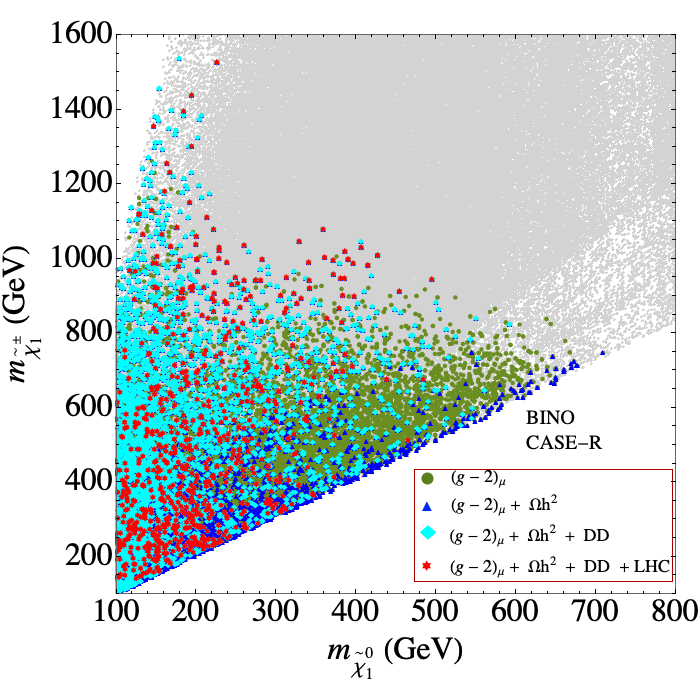
(a)

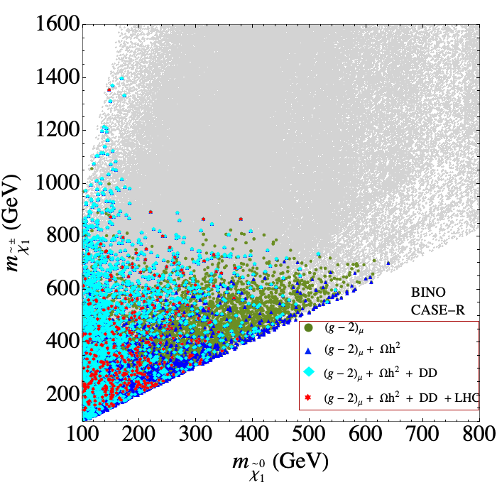
(b)

Figure 20: The results of our parameter scan in the $m_{\tilde{\chi}_{1}^{0}}-m_{\tilde{\chi}_{1}^{\pm}}$ plane for the $\tilde{l}$-coannihilation case-R scenario for current (left) and anticipated future limits (right) from $(g-2)_{\mu}$. The color coding is as in Fig. 18.

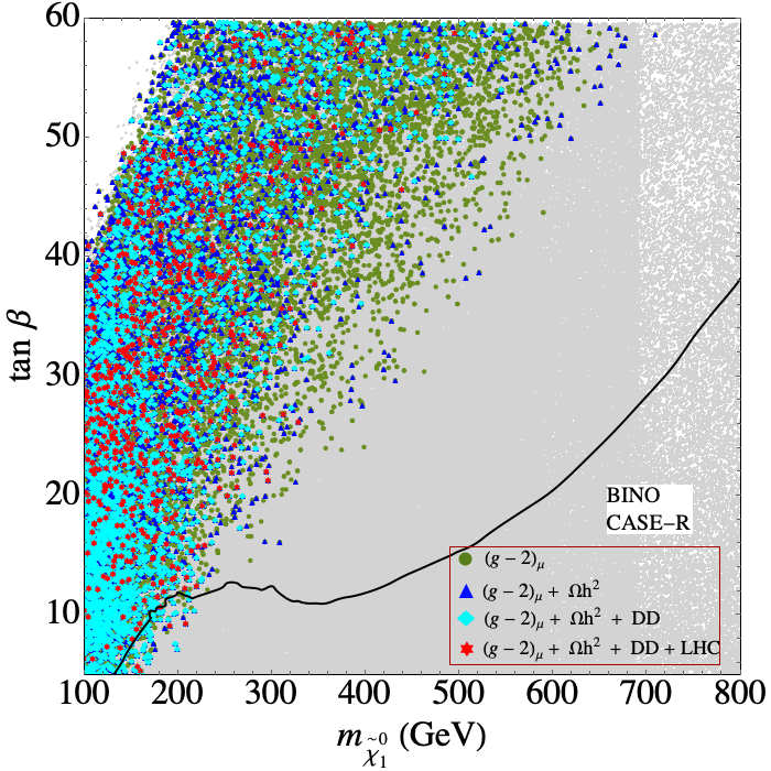
(a)

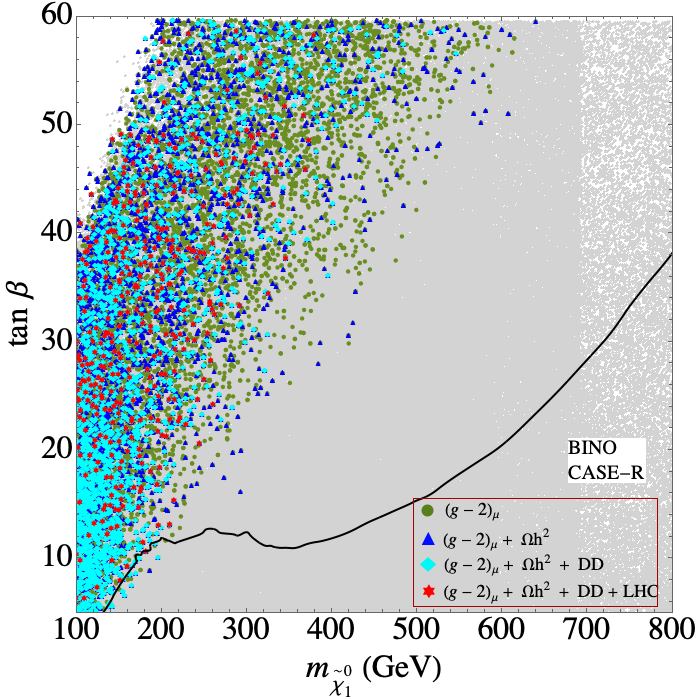
(b)

Figure 21: The results of our parameter scan in the $m_{\tilde{\chi}_{1}^{0}}$–$\tan\beta$ plane in the $\tilde{l}$-coannihilation case-R scenario for current (left) and anticipated future limits (right) from $(g-2)_{\mu}$. The color coding is as in Fig. 18. The black line indicates the current exclusion bounds for heavy MSSM Higgs bosons at the LHC (see text).

We finish our analysis of the $\tilde{l}^{\pm}$-coannihilation Case-R with the results in the $m_{\tilde{\chi}_{1}^{0}}$–$\tan\beta$ plane, presented in Fig. 21. The overall picture is similar to the previous cases shown above in Figs. 14, 17, and also qualitatively in agreement with the results found in Ref. [15]. Larger LSP masses are allowed for larger $\tan\beta$ values. On the other hand the combination of small $m_{\tilde{\chi}_{1}^{0}}$ and very large $\tan\beta$ values, $\tan\beta\;\raisebox{-3.00003pt}{$\stackrel{{\scriptstyle\displaystyle>}}{{\sim}}$}\;40$ leads to stau masses below the LSP mass, which we exclude for the CDM constraints. The LHC searches mainly affect parameter points with $\tan\beta\;\raisebox{-3.00003pt}{$\stackrel{{\scriptstyle\displaystyle<}}{{\sim}}$}\;20$. Larger $\tan\beta$ values induce a larger mixing in the third slepton generation, enhancing the probability for charginos to decay via staus and thus evading the LHC constraints. As before we also show the limits from $H/A$ searches at the LHC, where we set (as above) $m_{\tilde{\chi}_{1}^{0}}=M_{A}/2$, i.e. roughly to the requirement for $A$-pole annihilation, where points above the black lines are experimentally excluded. Comparing Case-R and Case-L, here for the current $(g-2)_{\mu}$ limit substantially less points are passing the current $(g-2)_{\mu}$ constraint below the black line, i.e. are potential candidates for $A$-pole annihilation. The masses reach only up to $\sim 200\,\,\mathrm{GeV}$. With the anticipated future $(g-2)_{\mu}$ limit hardly any point survives, leaving $A$-pole annihilation as a quite remote possibility with a strict upper bound on $m_{\tilde{\chi}_{1}^{0}}$.

5.4 Lowest and highest mass points

In this section we present some sample spectra for the five cases discussed in the previous subsections. For each case, higgsino DM, wino DM, bino/wino DM with $\tilde{\chi}_{1}^{\pm}$-coannihilation, $\tilde{l}^{\pm}$-coannihilation Case-L and Case-R, we present three parameter points that are in agreement with all constraints (red points): the lowest LSP mass, the highest LSP with current $(g-2)_{\mu}$ constraints, as well as the highest LSP mass with the anticipated future $(g-2)_{\mu}$ constraint. They will be labeled as “H1, H2, H3”, “W1, W2, W3”, "C1, C2, C3", "L1, L2, L3", "R1, R2, R3" for higgsino DM, wino DM, bino/wino DM with $\tilde{\chi}_{1}^{\pm}$-coannihilation, $\tilde{l}^{\pm}$-coannihilation Case-L and Case-R, respectively. While the points are obtained from "random sampling", nevertheless they give an idea of the mass spectra realized in the various scenarios. In particular, the highest mass points give a clear indication on the upper limits of the NLSP mass. It should be noted that the $\sigma_{p}^{\rm SI}$ values given below are scaled with a factor of ($\Omega_{\tilde{\chi}}h^{2}$/0.118) to account for the lower relic density.

In Tab. 1 we show the $3$ parameter points ("H1, H2, H3") from higgsino DM scenario, which are defined by the six scan parameters: $M_{1}$, $M_{2}$, $\mu$, $\tan\beta$ and the two slepton mass parameters, $m_{\tilde{l}_{L}}$ and $m_{\tilde{l}_{R}}$ (corresponding roughly to $m_{\tilde{e}_{1},\tilde{\mu}_{1}}$ and $m_{\tilde{e}_{2},\tilde{\mu}_{2}}$, respectively). Together with the masses and relevant BRs we also show the values of the DM observables and $a_{\mu}^{\rm SUSY}$. By definition of the scenario we have $\mu<M_{1},M_{2}$ and $m_{\tilde{\chi}_{1}^{0}}\sim m_{\tilde{\chi}_{2}^{0}}\sim m_{\tilde{\chi}_{1}^{\pm}}$ with the $\tilde{\chi}_{1}^{\pm}$ as NLSP. We find in all three points $M_{2}\ll M_{1}$, which can be understood from the $(g-2)_{\mu}$ constraint. For (relatively) small $\mu$ the chargino-sneutrino contribution, Eq. (5), is $\propto 1/M_{2}$ and thus becomes large for smaller $M_{2}$. Conversely, the neutralino-slepton contribution, Eq. (6), is $\propto M_{1}$ and thus becomes larger for larger $M_{1}$. As anticipated, the relic density is found to be quite low. For all of the three points, the decays of $\tilde{\chi}_{1}^{\pm}$ and $\tilde{\chi}_{2}^{0}$ to sleptons are not kinematically accessible. Therefore they mainly decay via off-shell sleptons and/or gauge-bosons to a pair of SM particles and the LSP. The sleptons represented by $\tilde{l}_{1}$ and $\tilde{l}_{2}$ decay to chargino/neutralino and the corresponding SM particle. The $\tilde{l}_{2}$ is mostly “right-handed” and thus decays preferably to a bino and an electron. However, this mode is kinematically open only for H3, leading to the observed $\tilde{l}_{2}$ decay pattern for H1 and H2.

Sample points	H1	H2	H3	Sample points	H1	H2	H3
$M_{1}$	1005	3414	3397	$\text{BR}(\tilde{\chi}_{2}^{0}\rightarrow\tilde{\chi}_{1}^{0}\gamma$	0.5	5	2.4
$M_{2}$	478	1165	1007	$\phantom{\text{BR}(\tilde{\chi}_{2}^{0}}\rightarrow\tilde{\chi}_{1}^{0}q\bar{q}$	51	42.5	41.4
$\mu$	124	472	454	$\phantom{\text{BR}(\tilde{\chi}_{2}^{0}}\rightarrow\tilde{\chi}_{1}^{0}l\bar{l}$	6	5.8	5.6
$\tan\beta$	56	51.6	52.8	$\phantom{\text{BR}(\tilde{\chi}_{2}^{0}}\rightarrow\tilde{\chi}_{1}^{0}\tau\bar{\tau}$	3	2.8	2.4
$m_{\tilde{l}_{L}}$	599	496	520	$\phantom{\text{BR}(\tilde{\chi}_{2}^{0}}\rightarrow\tilde{\chi}_{1}^{0}\nu\bar{\nu}$	18	17.7	17
$m_{\tilde{l}_{R}}$	744	3039	4402	$\phantom{\text{BR}(\tilde{\chi}_{2}^{0}}\rightarrow\tilde{\chi}_{1}^{\pm}q\bar{q}$	14	17.4	21
$m_{\tilde{\chi}_{1}^{0}}$	118.6	475	455	$\phantom{\text{BR}(\tilde{\chi}_{2}^{0}}\rightarrow\tilde{\chi}_{1}^{\pm}\nu_{l}l$	4.8	7	8
$m_{\tilde{\chi}_{2}^{0}}$	133	482	463	$\phantom{\text{BR}(\tilde{\chi}_{2}^{0}}\rightarrow\tilde{\chi}_{1}^{\pm}\nu_{\tau}\tau$)	2	1.7	2.4
$m_{\tilde{\chi}_{3}^{0}}\sim m_{\tilde{\chi}_{2}^{\pm}}$	515	1200	1043	$\text{BR}(\tilde{\chi}_{1}^{\pm}\rightarrow\tilde{\chi}_{1}^{0}\tau\nu_{\tau}$	7.8	0.1	0.4
$m_{\tilde{\chi}_{4}^{0}}$	993	3390	3372	$\phantom{\text{BR}(\tilde{\chi}_{1}^{\pm}}\rightarrow\tilde{\chi}_{1}^{0}l\nu_{l}$	25.6	38	37
				$\phantom{\text{BR}(\tilde{\chi}_{1}^{\pm}}\rightarrow\tilde{\chi}_{1}^{0}q\bar{q}^{\prime}$)	66.5	61.5	62.4
$m_{\tilde{\chi}_{1}^{\pm}}$	124	477	457.6	$\text{BR}(\tilde{l}_{1}\rightarrow\tilde{\chi}_{1}^{0}l$	5.7	57	51
$m_{\tilde{e}_{1},\tilde{\mu}_{1}}$	601	498	522	$\phantom{\text{BR}(\tilde{l}_{1}}\rightarrow\tilde{\chi}_{2}^{0}l$	1.9	4	5
$m_{\tilde{e}_{2},\tilde{\mu}_{2}}$	745	3040	4401	$\phantom{\text{BR}(\tilde{l}_{1}}\rightarrow\tilde{\chi}_{3}^{0}l$	29	-	-
$m_{\tilde{\tau}_{1}}$	600	498	522	$\phantom{\text{BR}(\tilde{l}_{1}}\rightarrow\tilde{\chi}_{1}^{\pm}\nu_{l}$	2.8	39	44
$m_{\tilde{\tau}_{2}}$	746	3040	4402	$\phantom{\text{BR}(\tilde{l}_{1}}\rightarrow\tilde{\chi}_{2}^{\pm}\nu_{l}$)	60	-	-
$m_{\tilde{\nu}}$	596	492	516	$\text{BR}(\tilde{l}_{2}\rightarrow\tilde{\chi}_{1}^{0}l$	59	64	-
$\Omega_{\tilde{\chi}}h^{2}$	0.003	0.036	0.024	$\phantom{\text{BR}(\tilde{l}_{2}}\rightarrow\tilde{\chi}_{2}^{0}l$	37	34	-
$a_{\mu}^{\rm SUSY}\times 10^{10}$	37.5	14.1	16.5	$\phantom{\text{BR}(\tilde{l}_{2}}\rightarrow\tilde{\chi}_{3}^{0}l$	3	1	-
$\sigma_{p}^{\rm SI}\times 10^{10}$	1	3.5	3.5	$\phantom{\text{BR}(\tilde{l}_{2}}\rightarrow\tilde{\chi}_{4}^{0}l$)	-	-	99.9

Table 1: The masses (in $\,\,\mathrm{GeV}$) and relevant BRs (%) of three points from the higgsino DM scenario, corresponding to the lowest LSP mass, the highest LSP mass with current $(g-2)_{\mu}$ constraints, as well as the highest LSP mass with the anticipated future $(g-2)_{\mu}$ constraint. Here $\tilde{l}\,(l)$ refers to $\tilde{e}\,(e)$ and $\tilde{\mu}\,(\mu)$ together. $\nu$ denotes $\nu_{e}$, $\nu_{\mu}$ and $\nu_{\tau}$ together. Only BRs above $0.1$ % are shown. The values of $(g-2)_{\mu}$ and DM observables are also shown. $\sigma_{p}^{\rm SI}$ is scaled with a factor of ($\Omega_{\tilde{\chi}}h^{2}$/0.118) and given in the units of pb.

In Tab. 2 we show the $3$ parameter points ("W1, W2, W3") from wino DM scenario, defined in terms of the same set of input parameters as the higgsino DM scenario. Together with the masses and relevant BRs we also show the values of the DM observables and $a_{\mu}^{\rm SUSY}$. By definition of the scenario we have $M_{2}<M_{1},\mu$ and $m_{\tilde{\chi}_{1}^{0}}\sim m_{\tilde{\chi}_{1}^{\pm}}$, i.e. the $\tilde{\chi}_{1}^{\pm}$ being the NLSP decaying dominantly as $\tilde{\chi}_{1}^{\pm}\to\tilde{\chi}_{1}^{0}\pi^{\pm}$, but also the decay to the LSP and $e\nu_{e}$ or $\mu\nu_{\mu}$ occurs (either with a soft pion or a soft charged lepton). As anticipated, the relic density is found to be quite low. The second lightest neutralino is found substantially heavier than the LSP, with a variety of decay channels to be open, diluting possible signals. The sleptons represented by $\tilde{l}_{1}$ and $\tilde{l}_{2}$ decay to chargino/neutralino and the corresponding SM particle with relevant BRs to charged leptons, which will be crucial for their detection. The $\tilde{l}_{2}$ is mostly “right-handed” and thus decays preferably to a bino and an electron (i.e. the neutralino in the decay is determined by the mass ordering of $\mu$ and $M_{1}$).

Sample points	W1	W2	W3	Sample points	W1	W2	W3
$M_{1}$	948	747	1061	$\text{BR}(\tilde{\chi}_{2}^{0}\rightarrow\tilde{l}_{1}l$	-	32.8	3.56
$M_{2}$	110	608	523	$\phantom{\text{BR}(\tilde{\chi}_{2}^{0}}\rightarrow{\tilde{\tau}_{1}}\tau$	-	19.4	18.6
$\mu$	313	1122	949	$\phantom{\text{BR}(\tilde{\chi}_{2}^{0}}\rightarrow\tilde{\nu}\nu$	-	44.4	0.12
$\tan\beta$	20.3	56.5	57.4	$\phantom{\text{BR}(\tilde{\chi}_{2}^{0}}\rightarrow\tilde{\chi}_{1}^{\pm}W$	70	3.2	52
$m_{\tilde{l}_{L}}$	557	679	656	$\phantom{\text{BR}(\tilde{\chi}_{2}^{0}}\rightarrow\tilde{\chi}_{1}^{0}Z$	27	-	1.8
$m_{\tilde{l}_{R}}$	356	1744	1559	$\phantom{\text{BR}(\tilde{\chi}_{2}^{0}}\rightarrow\tilde{\chi}_{1}^{0}h)$	3	-	24
$m_{\tilde{\chi}_{1}^{0}}$	100	602.8	517.7
$m_{\tilde{\chi}_{2}^{0}}$	320	745	948
$m_{\tilde{\chi}_{3}^{0}}\sim m_{\tilde{\chi}_{2}^{\pm}}$	328	1124	951	$\text{BR}(\tilde{\chi}_{1}^{\pm}\rightarrow\tilde{\chi}_{1}^{0}q\bar{q}^{\prime}$	67.4	73	74
$m_{\tilde{\chi}_{4}^{0}}$	950	1132	1070	$\phantom{\text{BR}(\tilde{\chi}_{1}^{\pm}}\rightarrow\tilde{\chi}_{1}^{0}e\nu_{e}$	22.9	27	26
				$\phantom{\text{BR}(\tilde{\chi}_{1}^{\pm}}\rightarrow\tilde{\chi}_{1}^{0}\mu\nu_{\mu})$	9.7	-	-
$m_{\tilde{\chi}_{1}^{\pm}}$	100.4	603	517.8	$\text{BR}(\tilde{l}_{1}\rightarrow\tilde{\chi}_{1}^{0}l$	32.5	33	33.4
$m_{\tilde{e}_{1},\tilde{\mu}_{1}}$	559	680	658	$\phantom{\text{BR}(\tilde{l}_{1}}\rightarrow\tilde{\chi}_{3}^{0}l$	1.4	-	-
$m_{\tilde{e}_{2},\tilde{\mu}_{2}}$	359	1745	1560	$\phantom{\text{BR}(\tilde{l}_{1}}\rightarrow\tilde{\chi}_{1}^{\pm}\nu_{l}$	61.6	67	66.6
$m_{\tilde{\tau}_{1}}$	358	676	653	$\phantom{\text{BR}(\tilde{l}_{1}}\rightarrow\tilde{\chi}_{2}^{\pm}\nu_{l})$	4.2	-	-
$m_{\tilde{\tau}_{2}}$	560	1746	1561
$m_{\tilde{\nu}}$	554	676	653	$\text{BR}(\tilde{l}_{2}\rightarrow\tilde{\chi}_{1}^{0}l$	30.4	-	-
$\Omega_{\tilde{\chi}}h^{2}$	3.6 $\times 10^{-4}$	0.014	0.009	$\phantom{\text{BR}(\tilde{l}_{2}}\rightarrow\tilde{\chi}_{2}^{0}l$	16.4	99.6	13
$a_{\mu}^{\rm SUSY}\times 10^{10}$	16.2	13.7	16.5	$\phantom{\text{BR}(\tilde{l}_{2}}\rightarrow\tilde{\chi}_{3}^{0}l$	53	-	-
$\sigma_{p}^{\rm SI}\times 10^{10}$	0.12	1.6	1.48	$\phantom{\text{BR}(\tilde{l}_{2}}\rightarrow\tilde{\chi}_{4}^{0}l)$	-	0.3	87

Table 2: The masses (in $\,\,\mathrm{GeV}$) and relevant BRs (%) of three points from the wino DM scenario, corresponding to the lowest LSP mass, the highest LSP mass with current $(g-2)_{\mu}$ constraints, as well as the highest LSP mass with the anticipated future $(g-2)_{\mu}$ constraint. The notation and units used are as in Tab. 1. $\tilde{\nu}\nu$ refers to all three generations (which in our sampling are mass degenerate). Only BRs above $0.1$ % are shown.

In Tab. 3 we show the $3$ parameter points ("C1, C2, C3") from $\tilde{\chi}_{1}^{\pm}$-coannihilation scenario, with the same definitions and notations as for the previous tables. We find that the $\tilde{\tau}$ is the NLSP in these three cases, and the combined contribution from $\tilde{\tau}$-coannihilation together with $\tilde{\chi}_{1}^{\pm}$-coannihilation brings the relic density to the ballpark value. For all of the three points, the decays of $\tilde{\chi}_{1}^{\pm}$ and $\tilde{\chi}_{2}^{0}$ to first two generations of sleptons are not kinematically accessible or strongly phase space suppressed. Therefore they decay with a very large BR to third generation charged sleptons and sneutrinos. This makes them effectively invisible to the LHC searches looking for electrons and muons in the signal. LHC analyses designed to specifically look for $\tau$-rich final states can prove beneficial to constrain these points, which are much less powerful, as discussed above. We refrain from showing results for ${\tilde{\tau}}$ decays, since the corresponding dedicated searches turn out to be weaker (and thus not effective) than other applicable searches.

Sample points	C1	C2	C3	Sample points	C1	C2	C3
$M_{1}$	138	592	528	$\text{BR}(\tilde{\chi}_{2}^{0}\rightarrow\tilde{\tau}_{1}\tau$	95.6	100	100
$M_{2}$	151	640	556	$\phantom{\text{BR}(\tilde{\chi}_{2}^{0}}\rightarrow\tilde{\nu}\nu$)	4.3	-	-
$\mu$	1113	1094	1032
$\tan\beta$	6.3	57	55	$\text{BR}(\tilde{\chi}_{1}^{\pm}\rightarrow\tilde{\tau}_{1}\nu_{\tau}$	96.3	100	100
$m_{\tilde{l}_{L}}=m_{\tilde{l}_{R}}$	167	678	616	$\phantom{\text{BR}(\tilde{\chi}_{1}^{\pm}}\rightarrow l\tilde{\nu}_{l}$	3	-	-
$m_{\tilde{\chi}_{1}^{0}}$	134	583	520	$\phantom{\text{BR}(\tilde{\chi}_{1}^{\pm}}\rightarrow\tau\tilde{\nu}_{\tau}$)	0.6	-	-
$m_{\tilde{\chi}_{2}^{0}}$	158	663	576
$m_{\tilde{\chi}_{3}^{0}}$	1123	1100	1039
$m_{\tilde{\chi}_{4}^{0}}\sim m_{\tilde{\chi}_{2}^{\pm}}$	1126	1107	1045	$\text{BR}(\tilde{l}_{1}\rightarrow\tilde{\chi}_{1}^{0}l$	32	74	33
$m_{\tilde{\chi}_{1}^{\pm}}$	158	662	578	$\phantom{\text{BR}(\tilde{l}_{1}}\rightarrow\tilde{\chi}_{2}^{0}l$	23	9	23
$m_{\tilde{e}_{1},\tilde{\mu}_{1}}$	173	680	618	$\phantom{\text{BR}(\tilde{l}_{1}}\rightarrow\tilde{\chi}_{1}^{\pm}\nu_{l}$)	45	17	44
$m_{\tilde{e}_{2},\tilde{\mu}_{2}}$	173	680	618
$m_{\tilde{\tau}_{1}}$	134	584	523
$m_{\tilde{\tau}_{2}}$	204	764	700
$m_{\tilde{\nu}}$	155	675	613	$\text{BR}(\tilde{l}_{2}\rightarrow\tilde{\chi}_{1}^{0}l)$	99.9	99.9	99.9
$\Omega_{\tilde{\chi}}h^{2}$	0.02	0.07	0.078
$a_{\mu}^{\rm SUSY}\times 10^{10}$	24	14.3	16.5
$\sigma_{p}^{\rm SI}\times 10^{10}$	0.083	1.09	1.18

Table 3: The masses (in $\,\,\mathrm{GeV}$) and relevant BRs (%) of three points from $\tilde{\chi}_{1}^{\pm}$-coannihilation scenario corresponding to the lowest LSP mass, the highest LSP mass with current $(g-2)_{\mu}$ constraints, as well as the highest LSP mass with the anticipated future $(g-2)_{\mu}$ constraint. The notation, definitions and units are as in Tab. 2. Only BRs above $0.1$ % are shown.

In Tab. 4 we show three parameter points ("L1, L2, L3") taken from $\tilde{l}^{\pm}$-coannihilation scenario Case-L, defined in the same way as in the $\tilde{\chi}_{1}^{\pm}$-coannihilation case. The character of the $\tilde{\chi}_{2}^{0}$ and $\tilde{\chi}_{1}^{\pm}$ depend on the mass ordering of $\mu$ and $M_{2}$ and are thus somewhat random. This leads to a large variation in the various BRs of these two particles, possibly diluting any signal involving a certain SM particle, such as a charged lepton. The selectrons or smuons, on the other hand, decay to the LSP and the corresponding SM lepton, which tend to be soft in this case, making way for compressed spectra searches at the LHC.

Sample points	L1	L2	L3	Sample points	L1	L2	L3
$M_{1}$	102	522	474	$\text{BR}(\tilde{\chi}_{2}^{0}\rightarrow\tilde{l}_{1}l$	22	19	26
$M_{2}$	1008	903	504	$\phantom{\text{BR}(\tilde{\chi}_{2}^{0}}\rightarrow\tilde{l}_{2}l$	1	-	-
$\mu$	675	896	1262	$\phantom{\text{BR}(\tilde{\chi}_{2}^{0}}\rightarrow\tilde{\tau}_{1}\tau$	14.4	45	25.6
$\tan\beta$	6.8	55.6	48.6	$\phantom{\text{BR}(\tilde{\chi}_{2}^{0}}\rightarrow\tilde{\tau}_{2}\tau$	1.6	4.4
$m_{\tilde{l}_{L}}$	118	601	483	$\phantom{\text{BR}(\tilde{\chi}_{2}^{0}}\rightarrow\tilde{\chi}_{1}^{0}h$	35	7.6	-
$m_{\tilde{l}_{R}}$	407	606	1024	$\phantom{\text{BR}(\tilde{\chi}_{2}^{0}}\rightarrow\tilde{\chi}_{1}^{0}Z$	11	0.5	-
$m_{\tilde{\chi}_{1}^{0}}$	97	513	466	$\phantom{\text{BR}(\tilde{\chi}_{2}^{0}}\rightarrow\tilde{\nu}\nu)$	15	23	48.6
$m_{\tilde{\chi}_{2}^{0}}$	675	860	525
$m_{\tilde{\chi}_{3}^{0}}$	686	904	1269
$m_{\tilde{\chi}_{4}^{0}}\sim m_{\tilde{\chi}_{2}^{\pm}}$	1045	975	1272	$\text{BR}(\tilde{\chi}_{1}^{\pm}\rightarrow\tilde{\nu}_{l}l$	21.6	19	33.4
$m_{\tilde{\chi}_{1}^{\pm}}$	674	860	525	$\phantom{\text{BR}(\tilde{\chi}_{1}^{\pm}}\rightarrow\tilde{\nu}_{\tau}\tau$	14	24	17
$m_{\tilde{e}_{1},\tilde{\mu}_{1}}$	126	602	485	$\phantom{\text{BR}(\tilde{\chi}_{1}^{\pm}}\rightarrow\tilde{l}_{1}\nu_{l}$	11	16	25
$m_{\tilde{e}_{2},\tilde{\mu}_{2}}$	407	608	1025	$\phantom{\text{BR}(\tilde{\chi}_{1}^{\pm}}\rightarrow\tilde{\tau}_{1}\nu_{\tau}$	6	33	24.5
$m_{\tilde{\tau}_{1}}$	124	519	468	$\phantom{\text{BR}(\tilde{\chi}_{1}^{\pm}}\rightarrow\tilde{\tau}_{2}\nu_{\tau}$	1	0.3	-
$m_{\tilde{\tau}_{2}}$	410	681	1033	$\phantom{\text{BR}(\tilde{\chi}_{1}^{\pm}}\rightarrow W\tilde{\chi}_{1}^{0})$	46	7.5	-
$m_{\tilde{\nu}}$	100	597	479
$\Omega_{\tilde{\chi}}h^{2}$	0.036	0.121	0.109	$\text{BR}(\tilde{l}_{1}\rightarrow\tilde{\chi}_{1}^{0}l)$	100	100	100
$a_{\mu}^{\rm SUSY}\times 10^{10}$	32.87	14	17.3	$\text{BR}(\tilde{l}_{2}\rightarrow\tilde{\chi}_{1}^{0}l)$	100	100	99.99
$\sigma_{p}^{\rm SI}\times 10^{10}$	0.25	2.8	0.45

Table 4: The masses (in $\,\,\mathrm{GeV}$) and relevant BRs (%) of three points from $\tilde{l}^{\pm}$-coannihilation scenario Case-L corresponding to the lowest LSP mass, the highest LSP mass with current $(g-2)_{\mu}$ constraints, as well as the highest LSP mass with the anticipated future $(g-2)_{\mu}$ constraint. The notation, definitions and units are as in Tab. 1. Only BRs above $0.1$ % are shown.

The masses, BRs and values of the $(g-2)_{\mu}$ and DM observables of the parameter point for the Case-R ("R1, R2, R3”) are shown in Tab. 5, defined in the same way as in the $\tilde{\chi}_{1}^{\pm}$-coannihilation case. As in the case-L the character of the $\tilde{\chi}_{2}^{0}$ and $\tilde{\chi}_{1}^{\pm}$ depend on the mass ordering of $\mu$ and $M_{2}$ and are thus somewhat random. In particular for the two high-mass points R2 and R3 the two mass parameters are relatively close, leading to larger mixings for these two states. This in turn leads to a larger variation in the various BRs of these two particles, possibly diluting any signal involving a certain SM particle, such as a charged lepton. The selectrons or smuons, on the other hand, decay preferably to the LSP and the corresponding SM lepton. As in case-L these tend to be soft, making way for compressed spectra searches at the LHC.

Sample points	R1	R2	R3	Sample points	R1	R2	R3
$M_{1}$	103	504	385	$\text{BR}(\tilde{\chi}_{2}^{0}\rightarrow\tilde{l}_{2}l$	1.8	0.4	-
$M_{2}$	212	1169	877	$\phantom{\text{BR}(\tilde{\chi}_{2}^{0}}\rightarrow\tilde{l}_{1}l$	-	4	24
$\mu$	971	958	976	$\phantom{\text{BR}(\tilde{\chi}_{2}^{0}}\rightarrow\tilde{\tau}_{2}\tau$	97	61	32
$\tan\beta$	6.6	59	59	$\phantom{\text{BR}(\tilde{\chi}_{2}^{0}}\rightarrow\tilde{\tau}_{1}\tau$	-	18.4	7
$m_{\tilde{l}_{L}}$	272	603	638	$\phantom{\text{BR}(\tilde{\chi}_{2}^{0}}\rightarrow\tilde{\chi}_{1}^{0}h$	0.9	11.5	2
$m_{\tilde{l}_{R}}$	112	598	438	$\phantom{\text{BR}(\tilde{\chi}_{2}^{0}}\rightarrow\tilde{\chi}_{1}^{0}Z$	0.2	1	0.3
$m_{\tilde{\chi}_{1}^{0}}$	100	496	380	$\phantom{\text{BR}(\tilde{\chi}_{2}^{0}}\rightarrow\tilde{\nu}\nu)$	-	3	34.5
$m_{\tilde{\chi}_{2}^{0}}$	222	953	877	$\text{BR}(\tilde{\chi}_{1}^{\pm}\rightarrow\tilde{l}_{1}\nu_{l}$	-	2	22.4
$m_{\tilde{\chi}_{3}^{0}}$	982	966	982	$\phantom{\text{BR}(\tilde{\chi}_{1}^{\pm}}\rightarrow\tilde{\tau}_{2}\nu_{\tau}$	96	37	30
$m_{\tilde{\chi}_{4}^{0}}\sim m_{\tilde{\chi}_{2}^{\pm}}$	986	1209	1011	$\phantom{\text{BR}(\tilde{\chi}_{1}^{\pm}}\rightarrow\tilde{\tau}_{1}\nu_{\tau}$	-	7	4
$m_{\tilde{\chi}_{1}^{\pm}}$	222	952	877	$\phantom{\text{BR}(\tilde{\chi}_{1}^{\pm}}\rightarrow\tilde{\nu}_{l}l$	-	4	24
$m_{\tilde{e}_{1},\tilde{\mu}_{1}}$	276	605	639	$\phantom{\text{BR}(\tilde{\chi}_{1}^{\pm}}\rightarrow\tilde{\nu}_{\tau}\tau$	-	38	17
$m_{\tilde{e}_{2},\tilde{\mu}_{2}}$	120	599	440	$\phantom{\text{BR}(\tilde{\chi}_{1}^{\pm}}\rightarrow W\tilde{\chi}_{1}^{0}$)	4	12	2.4
$m_{\tilde{\tau}_{2}}$	112	501	382	$\text{BR}(\tilde{l}_{1}\rightarrow\tilde{\chi}_{1}^{0}l)$	39	100	100
$m_{\tilde{\tau}_{1}}$	279	689	676	$\phantom{\text{BR}(\tilde{l}_{1}}\rightarrow\tilde{\chi}_{2}^{0}l$	21	-	-
$m_{\tilde{\nu}}$	265	600	634	$\phantom{\text{BR}(\tilde{l}_{1}}\rightarrow\tilde{\chi}_{1}^{\pm}\nu_{l})$	40	-	-
$\Omega_{\tilde{\chi}}h^{2}$	0.115	0.08	0.036
$a_{\mu}^{\rm SUSY}\times 10^{10}$	16.8	13	15.9	$\text{BR}(\tilde{l}_{2}\rightarrow\tilde{\chi}_{1}^{0}l)$	100	100	100
$\sigma_{p}^{\rm SI}\times 10^{10}$	0.35	1.24	0.27

Table 5: The masses (in $\,\,\mathrm{GeV}$) and relevant BRs (%) of three points from $\tilde{l}^{\pm}$-coannihilation scenario Case-R corresponding to the lowest LSP mass, the highest LSP mass with current $(g-2)_{\mu}$ constraints, as well as the highest LSP mass with the anticipated future $(g-2)_{\mu}$ constraint. The notation, definitions and units are as in Tab. 1. Only BRs above $0.1$ % are shown.

6 Prospects for future colliders

In this section we briefly discuss the prospects of the direct detection of the (relatively light) EW particles at the approved HL-LHC, the hypothetical upgrade to the HE-LHC, the potential future FCC-hh, and at a possible future $e^{+}e^{-}$ collider such as ILC [36, 37] or CLIC [38, 37]. We concentrate on the compressed spectra searches, relevant for higgsino DM, wino DM and bino/wino DM with $\tilde{\chi}_{1}^{\pm}$-coannihilation. Results for the future prospects for slepton coannihilation (although with the relic DM density taken as a direct measurement) can be found in Ref. [15].

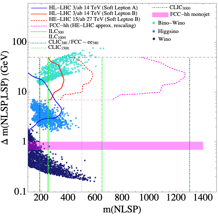
Figure 22: $m_{\tilde{\chi}_{1}^{\pm}}$–$\Delta m$ plane with anticipated limits from compressed spectra searches at the HL-LHC, the HE-LHC, FCC-hh and ILC500, ILC1000, CLIC380, CLIC1500, CLIC3000 (see text), original taken from Ref. [120]. Not included are disappearing track searches. Shown in blue, dark blue, turquoise are the points surviving all current constraints in the case of higgsino DM, wino DM and bino/wino DM with $\tilde{\chi}_{1}^{\pm}$-coannihilation, respectively.

In Fig. 22 we present our results in the $m_{\tilde{\chi}_{1}^{\pm}}$–$\Delta m$ plane (with $\Delta m:=m_{\tilde{\chi}_{1}^{\pm}}-m_{\tilde{\chi}_{1}^{0}}$), which was presented (in its original form, i.e. down to $\Delta m=0.7\,\,\mathrm{GeV}$) in Ref. [120] for the higgsino DM case, but also directly valid for the wino DM case [121] (see the discussion below). Shown are the following anticipated limits for compressed spectra searches:

• HL-LHC with $3\,\mbox{ab}^{-1}$ at $\sqrt{s}=14\,\,\mathrm{TeV}$:
  solid blue and solid red: di-lepton searches (with soft leptons) [124].

• HE-LHC with $15\,\mbox{ab}^{-1}$ at $\sqrt{s}=27\,\,\mathrm{TeV}$:
  red dashed: same analysis as in Ref. [124], but rescaled by 1.5 to take into account the higher energy [125].

• FCC-hh with $30\,\mbox{ab}^{-1}$ at $\sqrt{s}=100\,\,\mathrm{TeV}$:
  magenta dashed: same analysis as in Ref. [124], but rescaled to take into account the higher energy [120].
  solid magenta: mono-jet searches for very soft $\tilde{\chi}_{1}^{\pm}$ decays [125, 126] (see also the discussion in Ref. [121]), covering $\Delta m=0.7\,\,\mathrm{GeV}\ldots 1\,\,\mathrm{GeV}$. The upper limit can extend to higher values.

• ILC with $0.5\,\mbox{ab}^{-1}$ at $\sqrt{s}=500\,\,\mathrm{GeV}$ (ILC500):
  solid light green: $\tilde{\chi}_{1}^{\pm}\tilde{\chi}_{1}^{\pm}$ or $\tilde{\chi}_{2}^{0}\tilde{\chi}_{1}^{0}$ production, which is sensitive up to the kinematic limit [121] (and references therein).

• ILC with $1\,\mbox{ab}^{-1}$ at $\sqrt{s}=1000\,\,\mathrm{GeV}$ (ILC1000):
  gray dashed: $\tilde{\chi}_{1}^{\pm}\tilde{\chi}_{1}^{\pm}$ or $\tilde{\chi}_{2}^{0}\tilde{\chi}_{1}^{0}$ production, which is sensitive up to the kinematic limit [121] (and refrences therein).

• CLIC with $1\,\mbox{ab}^{-1}$ at $\sqrt{s}=380\,\,\mathrm{GeV}$ (CLIC380):
  very dark green dot-dashed: $\tilde{\chi}_{1}^{\pm}\tilde{\chi}_{1}^{\pm}$ or $\tilde{\chi}_{2}^{0}\tilde{\chi}_{1}^{0}$ production, which is sensitive up to the kinematic limit [120] (see also Ref. [121]).

• CLIC with $2.5\,\mbox{ab}^{-1}$ at $\sqrt{s}=1500\,\,\mathrm{GeV}$ (CLIC1500):
  green dot-dashed: $\tilde{\chi}_{1}^{\pm}\tilde{\chi}_{1}^{\pm}$ or $\tilde{\chi}_{2}^{0}\tilde{\chi}_{1}^{0}$ production, which is sensitive nearly up to the kinematic limit [120] (see also Ref. [121]).

• CLIC with $5\,\mbox{ab}^{-1}$ at $\sqrt{s}=3000\,\,\mathrm{GeV}$ (CLIC3000):
  dark green dot-dashed: $\tilde{\chi}_{1}^{\pm}\tilde{\chi}_{1}^{\pm}$ or $\tilde{\chi}_{2}^{0}\tilde{\chi}_{1}^{0}$ production, which is sensitive nearly up to the kinematic limit [120] (see also Ref. [121]).

Not shown in Fig. 22 are searches for disappearing tracks, which are relevant for very small mass differences, see Figs. 6 and 7. They cut out the lower edge of the dark blue points, wino DM. The life-time limits are expected to improve at the HL-LHC by a factor of $\sim 2$ [125], only slightly cutting into the still allowed region.

In the higgsino DM case (blue) it can be seen that the HL-LHC can cover part of the allowed parameter space, but that a full coverage can only be reached at a high-energy $e^{+}e^{-}$ collider with $\sqrt{s}\;\raisebox{-3.00003pt}{$\stackrel{{\scriptstyle\displaystyle<}}{{\sim}}$}\;1000\,\,\mathrm{GeV}$ (i.e. ILC1000 or CLIC1500). The wino DM case (dark blue), has larger production cross sections at $pp$ colliders. However, the $\Delta m$ is so small in this scenario that it largely escapes the HL-LHC searches (and the different production cross section turns out to be irrelevant). It can be expected that $\Delta m\;\raisebox{-3.00003pt}{$\stackrel{{\scriptstyle\displaystyle>}}{{\sim}}$}\;0.7\,\,\mathrm{GeV}$ can be covered with the monojet searches at the FCC-hh. Very low, but still allowed mass differences can be covered by the disappearing track searches. However, as for the higgsino DM case, also here a high-energy $e^{+}e^{-}$ collider will be necessary to cover the whole allowed parameter space. While the currently allowed points would require CLIC1500, a parameter space reduced by the HL-LHC disappearing track searches, resulting e.g. in $m_{\tilde{\chi}_{1}^{0}}\;\raisebox{-3.00003pt}{$\stackrel{{\scriptstyle\displaystyle<}}{{\sim}}$}\;500\,\,\mathrm{GeV}$ could be covered by the ILC1000.

The more complicated case for the future collider analysis is given by the bino/wino parameter points (turquoise), since the limits shown not only assume a small mass difference between $\tilde{\chi}_{1}^{0}$ and $\tilde{\chi}_{1}^{\pm}$, but also $pp$ production cross sections as for the higgsino case. For bino/wino DM these production cross sections turn out to be larger (as for the pure wino case), i.e. displaying the wino/bino points in Fig. 22 should be regarded as conservative with respect to the $pp$ based limits. Consequently, it is expected that the HE-LHC or “latest” the FCC-hh would cover this scenario entirely. On the other hand, the $e^{+}e^{-}$ limits should be directly applicable, and large parts of the parameter space will be covered by the ILC1000, and the entire parameter space by CLIC1500.

As discussed in Sect. 4.1 we have not considered explicitly the possibility of $Z$ or $h$ pole annihilation to find agreement of the relic DM density with the other experimental measurements. However, it should be noted that in this context an LSP with $M\sim m_{\tilde{\chi}_{1}^{0}}\sim M_{Z}/2$ or $\sim M_{h}/2$ (with $M=M_{1}$ or $M_{2}$ or $\mu$) would yield a detectable cross-section $e^{+}e^{-}\to\tilde{\chi}_{1}^{0}\tilde{\chi}_{1}^{0}\gamma$ in any future high-energy $e^{+}e^{-}$ collider. Furthermore, in the case of higgsino or wino DM, this scenario automatically yields other clearly detectable EW-SUSY production cross-sections at future $e^{+}e^{-}$ colliders. For bino/wino DM this would depend on the values of $M_{2}$ and/or $\mu$. We leave this possibility for future studies.

On the other hand, the possibility of $A$-pole annihilation was discussed for all five scenarios. While it appears a rather remote possibility (particularly for higgsino and wino DM), it cannot be fully excluded by our analysis. However, even in the “worst” case of $\tilde{l}^{\pm}$-coannihilation Case-L an upper limit on $m_{\tilde{\chi}_{1}^{0}}$ of $\sim 300\,\,\mathrm{GeV}$ can be set (about $\sim 40\,\,\mathrm{GeV}$ as as in the case with the relic DM density taken as a direct measurement [15]. While not as low as in the case of $Z$ or $h$-pole annihilation, this would still offer good prospects for future $e^{+}e^{-}$ colliders. We leave also this possibility for future studies.

7 Conclusions

The electroweak (EW) sector of the MSSM, consisting of charginos, neutralinos and scalar leptons can account for a variety of experimental data. Concerning the CDM relic abundance, where the MSSM offers a natural candidate, the lightest neutralino, $\tilde{\chi}_{1}^{0}$, while satisfying the (negative) bounds from DD experiments. Concerning the LHC searches, because of comparatively small EW production cross-sections, a relatively light EW sector of the MSSM is also in agreement with the latest experimental exclusion limits. Most importantly, the EW sector of the MSSM can account for the long-standing $3-4\,\sigma$ discrepancy of $(g-2)_{\mu}$. Improved experimental results are expected soon [3] by the publication of the Run 1 data of the “MUON G-2” experiment.

In this paper we assume that the $\tilde{\chi}_{1}^{0}$ provides MSSM DM candidate, where we take the DM relic abundance measurements [5] as an upper limit. We analyzed several SUSY scenarios, scanning the EW sector (chargino, neutralino and slepton masses as well as $\tan\beta$), taking into account all relevant experimental data: the current limit for $(g-2)_{\mu}$ , the relic density bound (as an upper limit), the DD experimental bounds, as well as the LHC searches for EW SUSY particles. Concerning the latter we included all relevant existing data, mostly relying on re-casting via CheckMATE, where several channels were newly implemented into CheckMATE [15].

Concretely, we analyzed five scenarios, depending on the hierarchy between $M_{1}$, $M_{2}$ and $\mu$ as well as the mechanism that brings the relic density in agreement with the experimental data. For $\mu<M_{1},M_{2}$ we have higgsino DM, for $M_{2}<M_{1},\mu$ wino DM, whereas for $M_{1}<M_{2},\mu$ one can have mixed bino/wino DM if $\tilde{\chi}_{1}^{\pm}$-coannihilation is responsible for the correct relic density (i.e. $M_{1}\;\raisebox{-3.00003pt}{$\stackrel{{\scriptstyle\displaystyle<}}{{\sim}}$}\;M_{2}$), or one can have bino DM if $\tilde{l}^{\pm}$-coannihilation yields the correct relic density, with the mass of the “left-handed” (“right-handed”) slepton close to $m_{\tilde{\chi}_{1}^{0}}$, Case-L (Case-R). Our scans naturally also consist “mixed” cases. Higgsino and wino DM, together with the $(g-2)_{\mu}$ constraint can only be fulfilled if the relic density is substantially smaller than the measured density. The other three scenarios can easily accommodate the relic DM density as direct measurement, which was analyzed in Ref. [15]. In the present analysis these three scenarios were extended to the case where the relic density is used only as an upper bound.

We find in all five cases a clear upper limit on $m_{\tilde{\chi}_{1}^{0}}$. These are $\sim 500\,\,\mathrm{GeV}$ for higgsino DM, $\sim 600\,\,\mathrm{GeV}$ for wino DM, while for $\tilde{\chi}_{1}^{\pm}$-coannihilation we find $\sim 600\,\,\mathrm{GeV}$, for $\tilde{l}^{\pm}$-coannihilation Case-L $\sim 500\,\,\mathrm{GeV}$ and for Case-R values up to $\sim 500\,\,\mathrm{GeV}$ are allowed. Similarly, upper limits to masses of the coannihilating SUSY particles are found as, $m_{\tilde{\chi}_{2}^{0}}\sim m_{\tilde{\chi}_{1}^{\pm}}\;\raisebox{-3.00003pt}{$\stackrel{{\scriptstyle\displaystyle<}}{{\sim}}$}\;510\,\,\mathrm{GeV}$ for higgsino DM, $m_{\tilde{\chi}_{1}^{\pm}}\;\raisebox{-3.00003pt}{$\stackrel{{\scriptstyle\displaystyle<}}{{\sim}}$}\;600\,\,\mathrm{GeV}$ for wino DM, $m_{\tilde{\chi}_{1}^{\pm}}\;\raisebox{-3.00003pt}{$\stackrel{{\scriptstyle\displaystyle<}}{{\sim}}$}\;650\,\,\mathrm{GeV}$ for bino/wino DM with $\tilde{\chi}_{1}^{\pm}$-coannihilation and $m_{\tilde{l}_{L}}\;\raisebox{-3.00003pt}{$\stackrel{{\scriptstyle\displaystyle<}}{{\sim}}$}\;600\,\,\mathrm{GeV}$ for bino DM case-L and $m_{\tilde{l}_{R}}\;\raisebox{-3.00003pt}{$\stackrel{{\scriptstyle\displaystyle<}}{{\sim}}$}\;600\,\,\mathrm{GeV}$ for bino DM case-R. For the latter, in the $\tilde{l}^{\pm}$-coannihilation case-R, the upper limit on the lighter $\tilde{\tau}$ is even lower, $m_{\tilde{\tau}_{2}}\;\raisebox{-3.00003pt}{$\stackrel{{\scriptstyle\displaystyle<}}{{\sim}}$}\;500\,\,\mathrm{GeV}$. The current $(g-2)_{\mu}$ constraint also yields limits on the rest of the EW spectrum, although much loser bounds are found. These upper bounds set clear collider targets for the HL-LHC and future $e^{+}e^{-}$ colliders.

In a second step we assumed that the new result of the Run 1 of the “MUON G-2” collaboration at Fermilab yields a precision comparable to the existing experimental result with the same central value. We analyzed the potential impact of the combination of the Run 1 data with the existing result on the allowed MSSM parameter space. We find that the upper limits on the LSP masses are decreased to about $\sim 480\,\,\mathrm{GeV}$ for higgsino DM, $\sim 500\,\,\mathrm{GeV}$ for wino DM, as well as $\sim 500\,\,\mathrm{GeV}$ for $\tilde{\chi}_{1}^{\pm}$-coannihilation, $\sim 450\,\,\mathrm{GeV}$ for $\tilde{l}^{\pm}$-coannihilation Case-L and $\sim 380\,\,\mathrm{GeV}$ in Case-R, sharpening the collider targets substantially. Similarly, the upper limits on the NLSP masses go down to about $m_{\tilde{\chi}_{2}^{0}}\sim m_{\tilde{\chi}_{1}^{\pm}}\;\raisebox{-3.00003pt}{$\stackrel{{\scriptstyle\displaystyle<}}{{\sim}}$}\;490\,\,\mathrm{GeV}$ for higgsino DM, $m_{\tilde{\chi}_{1}^{\pm}}\;\raisebox{-3.00003pt}{$\stackrel{{\scriptstyle\displaystyle<}}{{\sim}}$}\;600\,\,\mathrm{GeV}$ for wino DM, $m_{\tilde{\chi}_{1}^{\pm}}\sim 550\,\,\mathrm{GeV}$ for bino/wino DM with $\tilde{\chi}_{1}^{\pm}$-coannihilation, as well as $m_{\tilde{l}_{L}}\;\raisebox{-3.00003pt}{$\stackrel{{\scriptstyle\displaystyle<}}{{\sim}}$}\;550\,\,\mathrm{GeV}$ for bino DM case-L and $m_{\tilde{l}_{R}}\;\raisebox{-3.00003pt}{$\stackrel{{\scriptstyle\displaystyle<}}{{\sim}}$}\;440\,\,\mathrm{GeV}$, $m_{\tilde{\tau}_{2}}\;\raisebox{-3.00003pt}{$\stackrel{{\scriptstyle\displaystyle<}}{{\sim}}$}\;380\,\,\mathrm{GeV}$ for bino DM case-R.

For the three cases with a small mass difference between the lightest chargino and the LSP (higgsino DM, wino DM and bino/wino DM with $\tilde{\chi}_{1}^{\pm}$-coannihilation) we have also briefly analyzed the prospects for future collider searches, specially targeting these small mass differences. The results for the points surviving all (current) constraints have been displayed in the plane of the Next-to-LSP (in these cases $m_{\tilde{\chi}_{1}^{\pm}}$) vs. $\Delta m=m_{\tilde{\chi}_{1}^{\pm}}-m_{\tilde{\chi}_{1}^{0}}$, overlaid with the anticipated limits from future collider searches from HL-LHC, HE-LHC, FCC-hh, ILC and CLIC [120, 121]. (These limits are directly applicable to higgsino and wino DM, and likely to be overly conservative for bino/wino DM with $\tilde{\chi}_{1}^{\pm}$-coannihilation.) While parts of the parameter spaces can be covered by future $pp$ machines, a full exploration of the parameter space requires a future $e^{+}e^{-}$ colliders. Taking into account limits from future $e^{+}e^{-}$ machines, a center-of-mass energy of $\sqrt{s}=1\,\,\mathrm{TeV}$ will be sufficient to conclusively explore higgsino DM, wino DM and bino/wino DM with $\tilde{\chi}_{1}^{\pm}$-coannihilation.

While we have attempted to cover nearly the full set of possibilities that the EW spectrum of the MSSM presents, while being in agreement with all the various experimental constraints, our studies can be extended/completed in the following ways. One can analyze the cases of: (i) complex parameters in the chargino/neutralino sector (then also taking EDM constraints into account); (ii) different soft SUSY-breaking parameters in the three generations of sleptons, and/or between the left- and right-handed entries in the case of $\tilde{\chi}_{1}^{\pm}$-coannihilation; (iii) $A$-pole annihilation, in particular in the case of $\tilde{l}^{\pm}$-coannihilation for very low $m_{\tilde{\chi}_{1}^{0}}$ and $\tan\beta$ values; (iv) $h$- and $Z$-pole annihilation, which could be realized for sufficiently heavy sleptons. On the other hand, one can also restrict oneself further by assuming some GUT relations between, in particular, $M_{1}$ and $M_{2}$. We leave these analyses for future work.

In this paper we have analyzed in particular the impact of $(g-2)_{\mu}$ measurements on the EW SUSY spectrum. The current measurement sets clear upper limits on many EW SUSY particle masses. On the other hand we have also clearly demonstrated the potential of the upcoming measurements of the “MUON G-2” collaboration, which have a strong potential of sharpening the future collider experiment prospects. We are eagerly awaiting the new “MUON G-2” result to illuminate further the possibility of relatively light EW BSM particles.

Acknowledgments

We thank M. Berggren, J. List and D. Stöckinger for helpful discussions. We thank C. Schappacher for the calculation chargino/neutralino mass shifts. We thank T. Stefaniak for the evaluation of the latest direct search limits for heavy MSSM Higgs bosons in the $M_{h}^{125}(\tilde{\chi})$ scenario [110], using HiggsBounds [112, 113, 114, 115, 116]. I.S. gratefully thanks S. Matsumoto for the cluster facility. The work of I.S. is supported by World Premier International Research Center Initiative (WPI), MEXT, Japan. The work of S.H. is supported in part by the MEINCOP Spain under contract PID2019-110058GB-C21 and in part by the AEI through the grant IFT Centro de Excelencia Severo Ochoa SEV-2016-0597. The work of M.C. is supported by the project AstroCeNT: Particle Astrophysics Science and Technology Centre, carried out within the International Research Agendas programme of the Foundation for Polish Science financed by the European Union under the European Regional Development Fund.

References

- [1] A. Keshavarzi, D. Nomura and T. Teubner, Phys. Rev. D 101, no.1, 014029 (2020) [arXiv:1911.00367 [hep-ph]].
- [2] M. Davier, A. Hoecker, B. Malaescu and Z. Zhang, arXiv:1908.00921 [hep-ph].
-
[3]
See: https://theory.fnal.gov/events/event/
first-results-from-the-muon-g-2-experiment-at-fermilab . - [4] J. Grange et al. [Muon g-2 Collaboration], arXiv:1501.06858 [physics.ins-det].
- [5] N. Aghanim et al. [Planck Collaboration], arXiv:1807.06209 [astro-ph.CO].
- [6] D. S. Akerib et al. [LUX Collaboration], Phys. Rev. Lett. 118 (2017) no.2, 021303 [arXiv:1608.07648 [astro-ph.CO]].
- [7] X. Cui et al. [PandaX-II Collaboration], Phys. Rev. Lett. 119 (2017) no.18, 181302 [arXiv:1708.06917 [astro-ph.CO]].
- [8] E. Aprile et al. [XENON Collaboration], Phys. Rev. Lett. 121 (2018) no.11, 111302 [arXiv:1805.12562 [astro-ph.CO]].
- [9] H. Nilles, Phys. Rept. 110 (1984) 1.
- [10] R. Barbieri, Riv. Nuovo Cim. 11 (1988) 1.
- [11] H. Haber, G. Kane, Phys. Rept. 117 (1985) 75.
- [12] J. Gunion, H. Haber, Nucl. Phys. B 272 (1986) 1.
- [13] H. Goldberg, Phys. Rev. Lett. 50 (1983) 1419.
- [14] J. Ellis, J. Hagelin, D. Nanopoulos, K. Olive, M. Srednicki, Nucl. Phys. B 238 (1984) 453.
- [15] M. Chakraborti, S. Heinemeyer and I. Saha, Eur. Phys. J. C 80 (2020) 10, 984 [arXiv:2006.15157 [hep-ph]].
- [16] A. Bharucha, S. Heinemeyer and F. von der Pahlen, Eur. Phys. J. C 73 (2013) no.11, 2629 [arXiv:1307.4237 [hep-ph]].
- [17] A. Fowlie, K. Kowalska, L. Roszkowski, E. M. Sessolo and Y. L. S. Tsai, Phys. Rev. D 88 (2013), 055012 doi:10.1103/PhysRevD.88.055012 [arXiv:1306.1567 [hep-ph]].
- [18] T. Han, S. Padhi and S. Su, Phys. Rev. D 88 (2013) no.11, 115010 [arXiv:1309.5966 [hep-ph]].
- [19] K. Kowalska, L. Roszkowski, E. M. Sessolo and A. J. Williams, JHEP 06 (2015), 020 doi:10.1007/JHEP06(2015)020 [arXiv:1503.08219 [hep-ph]].
- [20] A. Choudhury and S. Mondal, Phys. Rev. D 94 (2016) no.5, 055024 [arXiv:1603.05502 [hep-ph]].
- [21] A. Datta, N. Ganguly and S. Poddar, Phys. Lett. B 763 (2016), 213-217 [arXiv:1606.04391 [hep-ph]].
- [22] M. Chakraborti, A. Datta, N. Ganguly and S. Poddar, JHEP 1711 (2017), 117 [arXiv:1707.04410 [hep-ph]].
- [23] K. Hagiwara, K. Ma and S. Mukhopadhyay, Phys. Rev. D 97 (2018) no.5, 055035 [arXiv:1706.09313 [hep-ph]].
- [24] T. T. Yanagida, W. Yin and N. Yokozaki, JHEP 06 (2020) 154 [arXiv:2001.02672 [hep-ph]].
- [25] W. Yin and N. Yokozaki, Phys. Lett. B 762 (2016) 72-79 [arXiv:1607.05705 [hep-ph]].
- [26] T. T. Yanagida, W. Yin and N. Yokozaki, JHEP 09, 086 (2016) [arXiv:1608.06618 [hep-ph]].
- [27] M. Chakraborti, U. Chattopadhyay and S. Poddar, JHEP 1709 (2017), 064 [arXiv:1702.03954 [hep-ph]].
- [28] E. A. Bagnaschi et al., Eur. Phys. J. C 75 (2015) 500 [arXiv:1508.01173 [hep-ph]].
- [29] A. Datta and N. Ganguly, JHEP 1801 (2019), 103 [arXiv:1809.05129 [hep-ph]].
- [30] P. Cox, C. Han and T. T. Yanagida, Phys. Rev. D 98, no.5, 055015 (2018) [arXiv:1805.02802 [hep-ph]].
- [31] P. Cox, C. Han, T. T. Yanagida and N. Yokozaki, JHEP 08 (2019), 097 [arXiv:1811.12699 [hep-ph]].
- [32] M. Abdughani, K. Hikasa, L. Wu, J. M. Yang and J. Zhao, JHEP 1911 (2019), 095 [arXiv:1909.07792 [hep-ph]].
- [33] M. Endo, K. Hamaguchi, S. Iwamoto and T. Kitahara, JHEP 2004 (2020), 165 [arXiv:2001.11025 [hep-ph]].
- [34] G. Pozzo and Y. Zhang, Phys. Lett. B789 (2019), 582-591 [arXiv:1807.01476 [hep-ph]].
- [35] P. Athron et al. [GAMBIT], Eur. Phys. J. C 79 (2019) no.5, 395 [arXiv:1809.02097 [hep-ph]].
- [36] H. Baer et al., The International Linear Collider Technical Design Report - Volume 2: Physics, arXiv:1306.6352 [hep-ph].
- [37] G. Moortgat-Pick et al., Eur. Phys. J. C 75 (2015) 8, 371 [arXiv:1504.01726 [hep-ph]].
-
[38]
L. Linssen, A. Miyamoto, M. Stanitzki and H. Weerts,
arXiv:1202.5940 [physics.ins-det];
H. Abramowicz et al. [CLIC Detector and Physics Study Collaboration], arXiv:1307.5288 [hep-ex];
P. Burrows et al. [CLICdp and CLIC Collaborations], CERN Yellow Rep. Monogr. 1802 (2018) 1 [arXiv:1812.06018 [physics.acc-ph]]. -
[39]
See: https://twiki.cern.ch/twiki/bin/view/AtlasPublic/
SupersymmetryPublicResults . - [40] See: https://twiki.cern.ch/twiki/bin/view/CMSPublic/PhysicsResultsSUS .
- [41] E. Bagnaschi et al., Eur. Phys. J. C 78 (2018) no.3, 256 [arXiv:1710.11091 [hep-ph]].
- [42] P. Slavich, S. Heinemeyer (eds.), E. Bagnaschi et al., arXiv:2012.15629 [hep-ph].
- [43] G. W. Bennett et al. [Muon g-2 Collaboration], Phys. Rev. D 73 (2006) 072003 [hep-ex/0602035].
- [44] M. Tanabashi et al. [Particle Data Group], Phys. Rev. D 98 (2018) no. 3, 030001.
- [45] T. Aoyama et al., [arXiv:2006.04822 [hep-ph]].
- [46] T. Aoyama, M. Hayakawa, T. Kinoshita and M. Nio, Phys. Rev. Lett. 109 (2012), 111808 [arXiv:1205.5370 [hep-ph]].
- [47] T. Aoyama, T. Kinoshita and M. Nio, Atoms 7 (2019) no.1, 28.
- [48] A. Czarnecki, W. J. Marciano and A. Vainshtein, Phys. Rev. D 67 (2003), 073006 [arXiv:hep-ph/0212229 [hep-ph]].
- [49] C. Gnendiger, D. Stöckinger and H. Stöckinger-Kim, Phys. Rev. D 88 (2013), 053005 [arXiv:1306.5546 [hep-ph]].
- [50] M. Davier, A. Hoecker, B. Malaescu and Z. Zhang, Eur. Phys. J. C 77 (2017) no.12, 827 [arXiv:1706.09436 [hep-ph]].
- [51] A. Keshavarzi, D. Nomura and T. Teubner, Phys. Rev. D 97 (2018) no.11, 114025 [arXiv:1802.02995 [hep-ph]].
- [52] G. Colangelo, M. Hoferichter and P. Stoffer, JHEP 02 (2019), 006 [arXiv:1810.00007 [hep-ph]].
- [53] M. Hoferichter, B. L. Hoid and B. Kubis, JHEP 08 (2019), 137 [arXiv:1907.01556 [hep-ph]].
- [54] A. Kurz, T. Liu, P. Marquard and M. Steinhauser, Phys. Lett. B 734 (2014), 144-147 [arXiv:1403.6400 [hep-ph]].
- [55] K. Melnikov and A. Vainshtein, Phys. Rev. D 70 (2004), 113006 [arXiv:hep-ph/0312226 [hep-ph]].
- [56] P. Masjuan and P. Sanchez-Puertas, Phys. Rev. D 95 (2017) no.5, 054026 [arXiv:1701.05829 [hep-ph]].
- [57] G. Colangelo, M. Hoferichter, M. Procura and P. Stoffer, JHEP 04 (2017), 161 [arXiv:1702.07347 [hep-ph]].
- [58] M. Hoferichter, B. L. Hoid, B. Kubis, S. Leupold and S. P. Schneider, JHEP 10 (2018), 141 [arXiv:1808.04823 [hep-ph]].
- [59] A. Gérardin, H. B. Meyer and A. Nyffeler, Phys. Rev. D 100 (2019) no.3, 034520 [arXiv:1903.09471 [hep-lat]].
- [60] J. Bijnens, N. Hermansson-Truedsson and A. Rodríguez-Sánchez, Phys. Lett. B 798 (2019), 134994 [arXiv:1908.03331 [hep-ph]].
- [61] G. Colangelo, F. Hagelstein, M. Hoferichter, L. Laub and P. Stoffer, JHEP 03 (2020), 101 [arXiv:1910.13432 [hep-ph]].
- [62] T. Blum, N. Christ, M. Hayakawa, T. Izubuchi, L. Jin, C. Jung and C. Lehner, Phys. Rev. Lett. 124 (2020) no.13, 132002 [arXiv:1911.08123 [hep-lat]].
- [63] G. Colangelo, M. Hoferichter, A. Nyffeler, M. Passera and P. Stoffer, Phys. Lett. B 735 (2014), 90-91 [arXiv:1403.7512 [hep-ph]].
- [64] T. Mibe [J-PARC g-2 Collaboration], Chin. Phys. C 34 (2010) 745.
- [65] S. Borsanyi et al., arXiv:2002.12347 [hep-lat].
- [66] C. Lehner and A. S. Meyer, Phys. Rev. D 101 (2020), 074515 [arXiv:2003.04177 [hep-lat]].
- [67] A. Crivellin, M. Hoferichter, C. A. Manzari and M. Montull, Phys. Rev. Lett. 125 (2020) no.9, 091801 [arXiv:2003.04886 [hep-ph]].
- [68] A. Keshavarzi, W. J. Marciano, M. Passera and A. Sirlin, Phys. Rev. D 102 (2020) no.3, 033002 [arXiv:2006.12666 [hep-ph]].
- [69] E. de Rafael, Phys. Rev. D 102 (2020) no.5, 056025 [arXiv:2006.13880 [hep-ph]].
- [70] T. Moroi, Phys. Rev. D 53 (1996) 6565 Erratum: [Phys. Rev. D 56 (1997) 4424] [hep-ph/9512396].
- [71] S. P. Martin and J. D. Wells, Phys. Rev. D 64 (2001) 035003 [hep-ph/0103067].
- [72] M. Badziak and K. Sakurai, JHEP 1910 (2019) 024 [arXiv:1908.03607 [hep-ph]].
- [73] P. Athron et al., Eur. Phys. J. C 76 (2016) no.2, 62 [arXiv:1510.08071 [hep-ph]].
- [74] P. von Weitershausen, M. Schafer, H. Stockinger-Kim and D. Stockinger, Phys. Rev. D 81 (2010), 093004 [arXiv:1003.5820 [hep-ph]].
- [75] H. Fargnoli, C. Gnendiger, S. Paßehr, D. Stöckinger and H. Stöckinger-Kim, JHEP 1402 (2014), 070 [arXiv:1311.1775 [hep-ph]].
- [76] M. Bach, J. h. Park, D. Stöckinger and H. Stöckinger-Kim, JHEP 1510 (2015), 026 [arXiv:1504.05500 [hep-ph]].
- [77] S. Heinemeyer, D. Stockinger and G. Weiglein, Nucl. Phys. B 690 (2004), 62-80 [arXiv:hep-ph/0312264 [hep-ph]].
- [78] S. Heinemeyer, D. Stockinger and G. Weiglein, Nucl. Phys. B 699 (2004), 103-123 [arXiv:hep-ph/0405255 [hep-ph]].
- [79] W. G. Hollik, G. Weiglein and J. Wittbrodt, JHEP 03 (2019), 109 [arXiv:1812.04644 [hep-ph]].
- [80] T. Robens, T. Stefaniak and J. Wittbrodt, Eur. Phys. J. C 80 (2020) no.2, 151 [arXiv:1908.08554 [hep-ph]].
- [81] M. Drees, H. Dreiner, D. Schmeier, J. Tattersall and J. S. Kim, Comput. Phys. Commun. 187 (2015), 227-265 [arXiv:1312.2591 [hep-ph]].
- [82] J. S. Kim, D. Schmeier, J. Tattersall and K. Rolbiecki, Comput. Phys. Commun. 196 (2015), 535-562 [arXiv:1503.01123 [hep-ph]].
- [83] D. Dercks, N. Desai, J. S. Kim, K. Rolbiecki, J. Tattersall and T. Weber, Comput. Phys. Commun. 221 (2017), 383-418 [arXiv:1611.09856 [hep-ph]].
- [84] G. Aad et al. [ATLAS Collaboration], Phys. Rev. D 101 (2020) no.5, 052005 [arXiv:1911.12606 [hep-ex]].
- [85] M. Aaboud et al. [ATLAS Collaboration], JHEP 06 (2018), 022 [arXiv:1712.02118 [hep-ex]].
- [86] A. M. Sirunyan et al. [CMS Collaboration], Phys. Lett. B 806 (2020), 135502 [arXiv:2004.05153 [hep-ex]].
- [87] G. Belanger, F. Boudjema, A. Pukhov and A. Semenov, Comput. Phys. Commun. 149 (2002), 103-120 [arXiv:hep-ph/0112278 [hep-ph]].
- [88] G. Belanger, F. Boudjema, A. Pukhov and A. Semenov, Comput. Phys. Commun. 176 (2007), 367-382 [arXiv:hep-ph/0607059 [hep-ph]].
- [89] G. Belanger, F. Boudjema, A. Pukhov and A. Semenov, Comput. Phys. Commun. 177 (2007), 894-895.
- [90] G. Belanger, F. Boudjema, A. Pukhov and A. Semenov, arXiv:1305.0237 [hep-ph].
- [91] K. J. Bae, H. Baer and E. J. Chun, Phys. Rev. D 89 (2014) no.3, 031701 [arXiv:1309.0519 [hep-ph]].
- [92] A. Sommerfeld, Ann. Phys. 403 (1931) 257.
- [93] H. Baer, V. Barger, P. Huang, A. Mustafayev and X. Tata, Phys. Rev. Lett. 109 (2012), 161802 [arXiv:1207.3343 [hep-ph]].
- [94] H. Baer, V. Barger and D. Mickelson, Phys. Rev. D 88 (2013) no.9, 095013 [arXiv:1309.2984 [hep-ph]].
- [95] H. Baer, V. Barger, M. Savoy and H. Serce, Phys. Lett. B 758 (2016), 113-117 [arXiv:1602.07697 [hep-ph]].
- [96] H. Baer, V. Barger, D. Sengupta and X. Tata, Eur. Phys. J. C 78 (2018) no.10, 838 [arXiv:1803.11210 [hep-ph]].
- [97] K. J. Bae, H. Baer, V. Barger and D. Sengupta, Phys. Rev. D 99 (2019) no.11, 115027 [arXiv:1902.10748 [hep-ph]].
- [98] H. Baer, V. Barger, S. Salam and D. Sengupta, Phys. Rev. D 102 (2020) no.7, 075012 [arXiv:2005.13577 [hep-ph]].
- [99] A. Delgado and M. Quirós, Phys. Rev. D 103 (2021) no.1, 015024 [arXiv:2008.00954 [hep-ph]].
- [100] E. Bagnaschi et al., Eur. Phys. J. C 77 (2017) no.4, 268 [arXiv:1612.05210 [hep-ph]].
- [101] T. Fritzsche, T. Hahn, S. Heinemeyer, F. von der Pahlen, H. Rzehak and C. Schappacher, Comput. Phys. Commun. 185 (2014), 1529-1545 [arXiv:1309.1692 [hep-ph]].
- [102] S. Heinemeyer and C. Schappacher, Eur. Phys. J. C 77 (2017) no.9, 649 [arXiv:1704.07627 [hep-ph]].
- [103] A. Djouadi, J. L. Kneur and G. Moultaka, Comput. Phys. Commun. 176 (2007) 426 [hep-ph/0211331].
- [104] Joint LEP2 SUSY Working Group, the ALEPH, DELPHI, L3 and OPAL Collaborations, see: http://lepsusy.web.cern.ch/lepsusy/ .
- [105] M. Muhlleitner, A. Djouadi and Y. Mambrini, Comput. Phys. Commun. 168 (2005) 46 [hep-ph/0311167].
- [106] G. Aad et al. [ATLAS Collaboration], Eur. Phys. J. C 80 (2020) no.2, 123 [arXiv:1908.08215 [hep-ex]].
- [107] H. Fukuda, N. Nagata, H. Otono and S. Shirai, Phys. Lett. B 781 (2018), 306-311 [arXiv:1703.09675 [hep-ph]].
- [108] J. Hisano, S. Matsumoto, M. M. Nojiri and O. Saito, Phys. Rev. D 71 (2005), 015007 [arXiv:hep-ph/0407168 [hep-ph]].
- [109] E. Aprile et al. [XENON], JCAP 11 (2020), 031 [arXiv:2007.08796 [physics.ins-det]].
- [110] E. Bagnaschi et al. Eur. Phys. J. C 79 (2019) no.7, 617 [arXiv:1808.07542 [hep-ph]].
- [111] G. Aad et al. [ATLAS Collaboration], Phys. Rev. Lett. 125 (2020) no.5, 051801 [arXiv:2002.12223 [hep-ex]].
- [112] P. Bechtle, O. Brein, S. Heinemeyer, G. Weiglein and K. E. Williams, Comput. Phys. Commun. 181 (2010), 138-167 [arXiv:0811.4169 [hep-ph]].
- [113] P. Bechtle, O. Brein, S. Heinemeyer, G. Weiglein and K. E. Williams, Comput. Phys. Commun. 182 (2011), 2605-2631 [arXiv:1102.1898 [hep-ph]].
- [114] P. Bechtle, O. Brein, S. Heinemeyer, O. Stål, T. Stefaniak, G. Weiglein and K. E. Williams, Eur. Phys. J. C 74 (2014) no.3, 2693 [arXiv:1311.0055 [hep-ph]].
- [115] P. Bechtle, S. Heinemeyer, O. Stål, T. Stefaniak and G. Weiglein, Eur. Phys. J. C 75 (2015) no.9, 421 [arXiv:1507.06706 [hep-ph]].
- [116] P. Bechtle, D. Dercks, S. Heinemeyer, T. Klingl, T. Stefaniak, G. Weiglein and J. Wittbrodt, Eur. Phys. J. C 80 (2020) no.12, 1211 [arXiv:2006.06007 [hep-ph]].
- [117] M. Ibe, S. Matsumoto and R. Sato, Phys. Lett. B 721 (2013), 252-260 [arXiv:1212.5989 [hep-ph]].
- [118] F. Ruppin, J. Billard, E. Figueroa-Feliciano and L. Strigari, Phys. Rev. D 90 (2014) no.8, 083510 [arXiv:1408.3581 [hep-ph]].
- [119] M. Aaboud et al. [ATLAS Collaboration], Eur. Phys. J. C 78 (2018) no.12, 995 [arXiv:1803.02762 [hep-ex]].
- [120] R. K. Ellis et al. [arXiv:1910.11775 [hep-ex]].
- [121] M. Berggren, arXiv:2003.12391 [hep-ph].
- [122] C. Natalia, F. Andrés, G. Alfredo, J. Will, S. Paul and T. cheng, arXiv:2102.10194 [hep-ph].
- [123] R. Capdevilla, F. Meloni, R. Simoniello and J. Zurita, arXiv:2102.11292 [hep-ph].
- [124] [ATLAS Collaboration], ATL-PHYS-PUB-2018-031.
- [125] X. Cid Vidal et al., CERN Yellow Rep. Monogr. 7 (2019), 585-865 [arXiv:1812.07831 [hep-ph]].
- [126] T. Golling et al. CERN Yellow Rep. (2017) no.3, 441-634 [arXiv:1606.00947 [hep-ph]].