Two-triplon excitations of the Kitaev-Heisenberg-Bilayer

Abstract

We study the spectrum of a bilayer of Kitaev magnets on the honeycomb lattice, coupled by Heisenberg exchange in the quantum-dimer phase at strong interlayer coupling. Using the perturbative Continuous Unitary Transformation (pCUT) we perform series expansion starting from the fully dimerized limit, to evaluate the elementary excitations, reaching up to and focusing on the two-triplon sector. In stark contrast to conventional bilayer quantum magnets, and because of the broken $SU(2)$-invariance, encoded in the intralayer directional compass-exchange, the bilayer Kitaev magnet is shown to exhibit a rich structure of two-triplon scattering-state continua, as well as several collective two-triplon (anti)bound states. Direct physical pictures for the occurrence of the latter are provided and the (anti)bound states are studied versus the stacking type, the spin components, and the exchange parameters. In addition to the two-triplon spectra, we investigate a corresponding experimental probe by evaluating the magnetic Raman-scattering intensity. We find a very strong sensitivity of this intensity on the two-triplon interactions and the scattering geometry, however a signal from the (anti)bound states appears only in very close proximity to the continuum.

I Introduction

Quantum phase transitions (QPTs) in local moment systems are of great interest [1]. In this context models are under intense scrutiny, comprising lattices of antiferromagnetic dimers, coupled by interdimer exchange networks. Tuning the interdimer exchange, these models allow for QPTs between states of weakly interacting singlets and various quantum phases determined by the type of interdimer network. Paradigmatic examples along this line include the square-lattice Heisenberg bilayer [2], three dimensional dimer networks [3], frustrated triangular and $J_{1}$-$J_{2}$ Heisenberg bilayers [4, 5], as well as the famous orthogonal dimer model [6]. Each of these models has been suggested to have corresponding realizations on the materials side, including BaCuSi₂O₆ [7], TlCuCl₃ [8], Ba₃Mn₂O₈ [9], Li₂VO(Si,Ge)O₄ [10], and SrCu₂(BO₃)₂ [11], respectively.

In unfrustrated antiferromagnetic Heisenberg bilayers, QPTs have been analyzed in great detail [2]. Three-dimensional O(3) universality and the critical coupling ratios have been firmly established. For frustrated interdimer exchange, less research has been performed. In this context, very recently, bilayers of the Kitaev quantum magnet on the honeycomb lattice, coupled by interlayer Heisenberg exchange, have attracted significant attention [12, 13, 14, 15]. A prime reason for this is, that in the limit of weak interlayer coupling, and instead of a local magnetic order parameter of Ginzburg-Landau type, the single layers of this magnet display a quantum spin liquid (QSL) state.

Indeed, the Kitaev single-layer magnet (KSLM) on the honeycomb lattice is one of the few spin models, in which a $\mathbb{Z}_{2}$ QSL can exactly be shown to exist [16]. The spin degrees of freedom of this model fractionalize in terms of mobile Majorana fermions coupled to a static $\mathbb{Z}_{2}$ gauge field [16, 17, 18, 19, 20]. In finite external magnetic fields, chiral Majorana edge-modes arise. Transition metal compounds with local Kramers doublets, induced by strong spin-orbit coupling may serve to realize the KSLM [21, 22], with $\alpha$-RuCl₃ [23] being among the most promising candidates. However, due to ubiquitous additional non-Kitaev interlayer exchange, only proximate Kitaev-QSLs have been reported so far [24, 25, 26, 27, 28]. Remarkable advances to engineer the KSLM in ultra cold gases, trapped in optical lattices have also been made [29].

Direct realizations of a Kitaev-Heisenberg bilayer magnet (KHBM) are yet lacking. However, excitonic magnetism in van Vleck $d^{4}$ Mott insulators, like Li₂RuO₃ [30] and Ag₃LiRu₂O₆ [31], has been suggested to effectively model very closely related physics [32, 34, 33].

The genuine KHBM [12, 13, 14, 15] displays a remarkably rich set of quantum phases, which depend decisively on the three different ways to stack the bilayer, the intralayer anisotropy of the Kitaev exchange, as well as the ratio of the dimer- to Kitaev-exchange [13]. In particular, and apart from the limiting cases of the weakly interacting quantum dimer phase (QDM) and the Kitaev QSL, an emergent Ising macro-spin phase as well as phase with spontaneous interlayer coherence and flux generation has been uncovered within the phase diagram [13].

Apart for the quantum phases, the elementary excitations in dimer magnets are of equal interest. This includes the dispersion [35, 36] and transport properties [37] of triplet excitations (triplons) in the QDM, as well as the fate of Goldstone and Higgs modes on approaching QPTs out of magnetically ordered phases [8, 38]. Apart from single triplon states, dimer magnets also allow to study multi triplon excitations including the formation of triplon (anti)bound states (ABS) [39, 40, 41], which may be observed in spectroscopies, like ESR [42], Raman [43], and inelastic neutron scattering [44].

For the KHBM some insight has been gained into the one-triplon dynamics in its QDM phase in Ref. [13]. An analysis of the two-triplon excitations and their interactions however is lacking. Therefore, in this work we step forward and study the two-triplon spectrum and the emergence of ABS in the KHBM. Moreover we consider the impact of these excitations on an experimental observable, i.e., on magnetic Raman spectroscopy. The outline of the paper is as follows. In Sec. II we detail the model. In Sec. III we describe our method of calculation, i.e., the perturbative Continuous Unitary Transformation (pCUT) and explain its application to the evaluation of one- and two-triplon excitations. Results for the one- and two-triplon spectra are presented in Sec. IV, separately for the isotropic (Sec. IV.2) and anisotropic case (Sec. IV.3). The calculation of dynamical correlation functions of observables and our findings for the Raman response are described in Sec. V. We conclude in Sec. VI. Several technical aspects are deferred to appendices A, B and C.

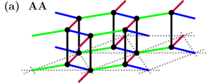
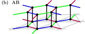
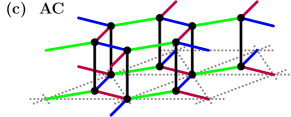
Figure 1: The KHBM lattice. Solid dots: spin-$1/2$ operators. Solid green, blue, red, and black bonds: $xx$, $yy$, $zz$ Ising, and Heisenberg exchange, $J_{\alpha}$, and $J_{\perp}$, respectively. (a), (b), and (c): AA, AB, and AC stacking.

II Model

The Hamiltonian of the KHBM reads

$$H=H_{0}+H_{I}$$ (1)

$$H_{0}=J_{\perp}\sum_{\bm{\rho}_{j=1,2}}\vec{S}_{\bm{\rho}_{j},1}\cdot\vec{S}_{\bm{\rho}_{j},2}$$

$$H_{I}=\sum_{\mathbf{r},\alpha,L}J_{\alpha}S^{\alpha}_{\mathbf{r},L}S^{\alpha}_{\mathbf{r}+\bm{\delta}_{\alpha}^{L},L}$$

where $\vec{S}=\{S^{\alpha}\}$ with $\alpha=x,y,z$ are spin-1/2 operators, $J_{\perp}$ and $J_{\alpha}$ are the Heisenberg interlayer and Kitaev intralayer exchange, respectively. In this work we focus on antiferromagnetic (ferromagnetic) interlayer (intralayer) exchange $J_{\perp}>0$ ($J_{\alpha}<0$). $L=1,2$ labels the two layers, with ${\bf r}=n_{1}{\bf R}_{1}+n_{2}{\bf R}_{2}$ running over the sites of the triangular lattice where ${\bf R}_{1[2]}=(1,0),\,[(\frac{1}{2},\frac{\sqrt{3}}{2})]$, with $n_{1,2}\in\mathbb{Z}$, and $\bm{\delta}^{1}_{\alpha}=(\frac{1}{2},\frac{1}{2\sqrt{3}}),$ $(-\frac{1}{2},\frac{1}{2\sqrt{3}})$, $(0,-\frac{1}{\sqrt{3}})$ refer to the honeycomb basis sites of layer $1$, tricoordinated to each bravais lattice site. $\bm{\rho}_{j=1,2}=(\mathbf{r},\mathbf{r}+\bm{\delta}^{1}_{x})$ encodes the basis of the honeycomb lattice, with ${\bf 0}_{j}=({\bf 0},\bm{\delta}^{1}_{x})$.

The model allows various stackings, by setting $\bm{\delta}^{2}_{\alpha}$ to certain permutations of $\bm{\delta}^{1}_{\alpha}$ with respect to $\alpha$. More specifically, and as shown in Fig. 1, the so-called AA-stacking results from $\bm{\delta}^{2}_{\alpha}=\bm{\delta}^{1}_{\alpha}$, AB-stacking is obtained from $\bm{\delta}^{2}_{x,y,z}=\bm{\delta}^{1}_{z,x,y}$, i.e., a 120° rotation, and finally AC-stacking refers to $\bm{\delta}^{2}_{x,y,z}=\bm{\delta}^{1}_{x,z,y}$, i.e., a mirror refection along one of the Ising bonds. For anisotropic Ising exchange, i.e., $J_{\alpha}\neq J_{\alpha^{\prime}}$, it may be preferable to further sub-categorize these stackings [13].

III Method

The KHBM comprises at least two limiting quantum phases which are adiabatically disjoint, i.e., are a separated by a QPT. For $|J_{\alpha}/J_{\perp}|\ll 1$ a QDM of weakly interacting antiferromagnetic dimers prevails. The dynamics of its elementary triplon excitations strongly depends on the stacking. In particular in the AA stacking the one-triplon excitations remain dispersionless for all values of $J_{\alpha}/J_{\perp}$ due to an extensive number conserved quantities build from the $\mathbb{Z}_{2}$ plaquettes of the two KSLMs, effectively locking the triplons on NN dimer pairs [12, 13]. For $|J_{\alpha}/J_{\perp}|\gg 1$, two decoupled Kitaev $\mathbb{Z}_{2}$ QSLs occur with Majorana fermion and vison excitations. Between these, and at intermediate coupling $|J_{\alpha}/J_{\perp}|\sim 1$ additional quantum phases have been discovered [13]. Our prime goal for the remainder of this work is to stay within the QDM and focus on its two-triplon excitations, their interactions, the potential formation of bound states and possible consequences for observable spectroscopic probes.

The limit $|J_{\alpha}/J_{\perp}|\ll 1$ is amenable to analytic series expansions (SE) by the perturbative Continuous Unitary Transformation (pCUT), which is our method of choice. The prime ingredient of this method is, that $H_{0}$ has a non-degenerate ground state and an equidistant ladder spectrum with interlevel spacing $J_{\perp}$, the energy levels of which carry a monotonously increasing integer quantum, or so-called particle number $Q$. For the present $H_{0}$, $Q$ refers to the number of excited triplons, which for each dimer we set to be

$$\ket{t_{x}}=- (\ket{\uparrow\uparrow}-\ket{\downarrow\downarrow})/\sqrt{2}\,,$$ (2)

$$\ket{t_{y}}=i (\ket{\uparrow\uparrow}+\ket{\downarrow\downarrow})/\sqrt{2}\,,$$

$$\ket{t_{z}}= (\ket{\uparrow\downarrow}+\ket{\downarrow\uparrow})/\sqrt{2}\,,$$

and refer to them as $x$-, $y$- and $z$-triplons hereafter. $Q=0$ refers to the product ground-state $|\rangle=\prod_{\bm{\rho}_{l}}|s_{\bm{\rho}_{l}}\rangle$ of singlets. One- and two-triplon states, i.e., $Q=1$ and $2$, are $|\bm{\rho}_{l}\alpha\rangle=|t_{\bm{\rho}_{l}\alpha}\rangle\otimes\prod_{\bm{\rho}_{j}\neq\bm{\rho}_{l}}|s_{\bm{\rho}_{j}}\rangle$ and $|\bm{\rho}_{j},\bm{\rho}_{l},\alpha\beta\rangle=|t_{\bm{\rho}_{j}\alpha}t_{\bm{\rho}_{l}\beta}\rangle\otimes\prod_{\bm{\rho}_{n}\neq\bm{\rho}_{j},\bm{\rho}_{l}}|s_{\bm{\rho}_{n}}\rangle$. In general the perturbation $H_{I}$ mixes different Q-sectors, i.e., the block-diagonal form of $H_{0}$ with respect to the triplon number is not conserved for $H$. Based on the ladder spectrum of $H_{0}$ however, a unitarily equivalent effective Hamiltonian $H_{\mathrm{eff}}=U^{\dagger}HU$ can be constructed which remains $Q$-diagonal, using the flow equation method of Wegner [45]. This methods provides the link to SE, as it is implemented perturbatively order by order in $H_{I}$, leading to

$$H_{\mathrm{eff}}=H_{0}+\sum_{l,m,n}^{\infty}C_{l,m,n}J_{x}^{l}J_{y}^{m}J_{z}^{n},$$ (3)

where $C_{l,m,n}$ are weighted products of terms in $H_{I}$, comprising $l+m+n$ non-local creations(destructions) of triplons which conserve the $Q$-number. The weights are determined by recursive differential equations. Details can be found in Refs. [46, 47, 48].

$Q$-number conservation allows to obtain the spectrum of $H$ from the irreducible matrix elements of $H_{\rm eff}$ with respect to the eigenstates of $H_{0}$. The ground state, i.e., $Q=0$, energy is $E_{0}=\langle|H_{\rm eff}|\rangle$. The one-triplon, i.e., $Q=1$, dispersion results from ${\bf E}_{\mathbf{k},jl,\alpha\beta}=\sum_{\bf r}e^{i\bm{\rho}_{j}\cdot{\bf k}}\langle\bm{\rho}_{j}\alpha|H_{\rm eff}|{\bf 0}_{l}\beta\rangle-\delta_{\bm{\rho}_{j}{\bf 0}_{l}}\delta_{\alpha\beta}E_{0}^{\text{cl}}$. In view of the two-site basis $j=1,2$ and the spin index $\alpha$, this is a $6\times 6$-matrix. However, as discussed in appendix A, the one-triplon hopping matrix elements are diagonal regarding the triplon components, leaving three $2\times 2$ dispersions, with roots $E_{\mathbf{k},i=1,2,\alpha}$, which can be determined analytically [13].

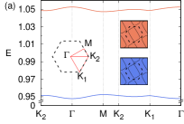
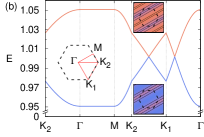
Figure 2: Solid blue(orange) line: one-triplon dispersion $E_{\mathbf{k},i=1(2),\alpha}$ for (a) $\alpha=x$-triplons and (b) $\alpha=y[z]$-triplons in AC-stacking at $J=-0.1J_{\perp}$ along high-symmetry lines of BZ. Insets: constant energy surfaces.

The $Q=2$, i.e., the two-triplon problem is more challenging [47, 48]. First, the irreducible two-triplon interaction is evaluated. Primarily this requires calculation of the matrix elements $\langle\bm{\rho}^{\prime}_{j^{\prime}},\bm{\rho}^{\prime}_{j^{\prime}}+\bm{\tau}^{\prime}_{l^{\prime}},\alpha^{\prime}\beta^{\prime}|H_{\rm eff}|\bm{\rho}_{j},\bm{\rho}_{j}+\bm{\tau}_{l},\alpha\beta\rangle$ for initial (final) two-triplon positions $\bm{\rho}^{(\prime)}_{j^{(\prime)}},\bm{\rho}^{(\prime)}_{j^{(\prime)}}+\bm{\tau}^{(\prime)}_{l^{(\prime)}}$ and triplon components $\alpha^{(\prime)}\beta^{(\prime)}$. Again, the subscripts $j,l=1,2$ label the honeycomb basis. Second, using translational invariance, a two-triplon Hamiltonian matrix $h_{\bf K}(\bm{\tau}^{\prime}_{l^{\prime}},\bm{\tau}_{l},\alpha^{\prime}\beta^{\prime},\alpha\beta)$ is set up from this, between two-triplon states $|{\bf K},\bm{\tau}_{l},\alpha\beta\rangle$, classified according to total momentum ${\bf K}$, two-triplon separation $\bm{\tau}_{l}$, and spin components $\alpha\beta$. Third, $h_{\bf K}(\bm{\tau}^{\prime}_{l^{\prime}},\bm{\tau}_{l},\alpha^{\prime}\beta^{\prime},\alpha\beta)$, comprising analytical matrix elements from the SE, is diagonalized numerically on sufficiently large systems.

In this context it is essential to understand the physics of $h_{\bf K}(\bm{\tau}^{\prime}_{l^{\prime}},\bm{\tau}_{l},\alpha^{\prime}\beta^{\prime},\alpha\beta)$. Namely, since it describes a two-body scattering problem for each ${\bf K}$, it is a banded matrix regarding $\bm{\tau}^{\prime}_{l^{\prime}},\bm{\tau}_{l}$. I.e., only in its upper left corner, for two-triplon separations $|\bm{\tau}^{(\prime)}_{l^{(\prime)}}|<d_{I}$, less than a characteristic distance, actual interactions occur. On the remainder of the band diagonal, free scattering states reside. This knowledge directly allows to eliminate any finite size effects of the numerical solution of this two-body scattering problem. We emphasize, that the systems involved in this final numerical step of the pCUT procedure easily comprise more than several hundred sites.

Similar to the one-triplon case, simplifications apply to the two-triplon Hamiltonian regarding its $9\times 9$ spin structure. In fact, non-zero irreducible matrix elements arise only for $\alpha^{\prime}\beta^{\prime}=\alpha\beta$ with $\alpha\beta$ one out of $(x,y)$, $(y,z)$ and $(z,x)$, or within the $3\times 3$ block of $\alpha^{(\prime)}\beta^{(\prime)}=[(x,x)$, $(y,y)$, $(z,z)]$. For additional details on the $Q=2$ case, see appendix A.

All evaluations of matrix elements of $H_{\rm eff}$, referred to in the preceding, are carried out on suitably chosen linked cluster graphs of the lattice. A description of this is deferred to appendix B.

IV One- and Two-triplon excitations

In this section we present our findings for the excitation spectra. As compared to conventional bilayer quantum magnets and as a consequence of the anisotropic Ising-type Kitaev exchange as well as the stacking options, we find these spectra to have a remarkably rich structure. Our main focus is on the two-triplon dynamic. However, and to determine the irreducible two-triplon interactions, also the ground state energy and the one-triplon spectra of the KHBM need to be known. These have been analyzed in Ref. [13]. For clarity, we revisit selected aspects of the latter results first.

IV.1 One-triplon dispersion

Here we remain with the AC-stacking. Figs. 2(a) and (b) display the dispersions $E_{\mathbf{k},i,\alpha}$ and the constant energy surfaces of the x- and y-/z-triplons, at $O(9)$ respectively. Each figure contains two dispersions, referring to the two-site basis. The plots evidences, that for a given type of stacking, rather distinct one-triplon dispersions can arise, depending on the type of triplon. This is a direct consequence of the directionally dependent Kitaev exchange and does not only pertain to the kinetic energy, but also induces an effective dimensionality. E.g., in the AC case, x-triplons acquire a non-zero hopping matrix element only at $O(2)$ of the SE and remain almost localized on the dimers linked by $S^{x}S^{x}$-exchange in Fig. 1(c). In contrast, the y-/z-triplons disperse at $O(1)$, however, their hopping matrix elements are locked to the zig-zag ladder in Fig.1(c), providing them with an identical and effectively 1D dispersion. For additional properties of the one-triplon excitations we refer to Ref. [13].

One information, important for the two-triplon spectrum, which can be read off directly from the one-triplon dispersion, is the support of the non-interacting two-triplon continuum. Namely, at fixed total momentum ${\bf K}$ it refers to the range of all energies $[E_{\mathbf{K}-\mathbf{q},i,\alpha}+E_{\mathbf{q},j,\beta}]$ with $\mathbf{q}\in\text{BZ}$.

IV.2 Isotropic Kitaev exchange

Now we turn to the two-triplon spectra, focusing on the isotropic case $J_{x,y,z}=J$ first. We begin with the AC-stacking and discuss a central result of our work in Fig. 3. This displays the eigenenergies obtained from the numerical diagonalization of the two-triplon subsector of the effective pCUT Hamiltonian in the $(y,z)$ channel, described in Sec. III, and obtained at $O(9)$ and $O(8)$ of the SE for one and two-triplon matrix elements, respectively. The spectrum is shown along various high-symmetry directions for the total two-triplon momentum in the BZ. Several comments are in order. First, a broad continuum is visible, which refers to the energy range of the two-triplon scattering states, comprising renormalized one-triplon dispersions as in Fig. 2. Second, there are clearly visible eigenenergies outside of the continuum, both below and above. These are the sought-for bonding and antibonding collective two-triplon states. We find these ABS for all coupling strengths within the convergence radius of the series and for all total momenta $\mathbf{K}$ investigated.

Third, and to prove the (anti)bonding nature of these states, we analyze not only the energies of the two-triplon states, but also their wave functions versus the relative inter triplon separation $\bm{\tau}_{l}$. One representative case is shown in Fig. 3 for each of the bonding, the antibonding, and the scattering-states spectral regions. The main difference between the former two and the latter is, that the ABS show a strong localization versus $\bm{\tau}_{l}$, while the scattering states are rather evenly distributed, with at most short wave-length oscillations.

Finally we emphasize, that in stark contrast to conventional bilayer spin models [39, 40], the KHBM’s spectrum of ABS does not separate into channels with well-defined total spin quantum-numbers, because of its broken $SU(2)$ invariance.

(a)                                                                  .

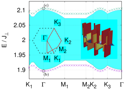
(b)                                  (c)                                 .

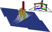
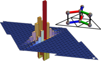
Figure 3: Panel (a): Two-triplon spectrum versus total momentum in $(y,z)$ channel along high-symmetry path of BZ for AC-stacking at $J=-0.1J_{\perp}$. Solid cyan region: Scattering state continuum. (Green)Magenta crosses: (Anti)Bound states (ABS). Panels (b) and (c): $yz$-component of wave function of ABS at total momentum ${\bf K}=\Gamma$, i.e., energies (b) and (c) in panel (a), versus real space coordinate $\bm{\tau}_{l}$ ($zy$-component provides identical information). Center of 2D plotting planes refer to $\bm{\tau}_{l}={\bf 0}_{1}$ and real-space bond-geometry is for reference. Analogous display within solid cyan region: Wave function of representative scattering state. System size: $18\times 18$ cells.

The existence of the AC $(y,z)$ ABS in the KHBM allows for a qualitative understanding. As noted in Sec. IV.1, the y- and z-triplons in the AC-stacking spread essentially in 1D along the $S^{y(z)}S^{y(z)}$ zigzag chains. One may now envisage an (anti)symmetric linear combination $\ket{\Psi_{\pm}}$ of the corresponding Wannier states $\ket{x}_{a}$, $\ket{y}_{b}$ on two dimers, linked by $S^{x}_{a,L}S^{x}_{b,L}$ intralayer exchange bonds

$$\ket{\Psi_{\pm}}=\ket{y,z}_{ab}\pm\ket{z,y}_{ab}\,.$$ (4)

These are eigenstates of the local intralayer $x$-exchange, combined between both layers

$$J_{x}(\sum_{L=1,2}S^{x}_{a,L}S^{x}_{b,L})\ket{\Psi_{\pm}}=\mp\frac{1}{2}J_{x}\ket{\Psi_{\pm}}$$ (5)

This lowest order on-bond (repulsion)attraction by $(+)-J$/2 is the reason for the formation of the ABS. As our results show this general relation holds true even for higher order SE. The preceding is corroborated by the two figures regarding the (anti)bound wavefunctions in Fig. 3(b) and 3(c). In fact, their probability amplitudes are confined to both triplons being on neighboring y/z-zigzag chains coupled by intralayer $S^{x}S^{x}$ bonds. As to be expected the wavefunction amplitudes get monotonously smaller for larger triplon distances because higher order coupling terms are needed to introduce two-triplon interactions at larger distances.

(a)                                                                  .

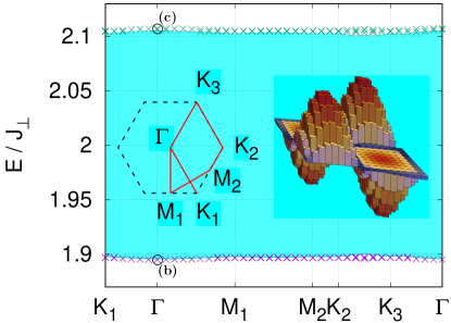
(b)                                  (c)                                 .

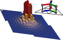
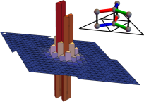
Figure 4: Panel (a): Two-triplon spectrum versus total momentum in the $(x,x),(y,y),(z,z)$-sector along high-symmetry path of BZ for AC-stacking at $J=-0.1J_{\perp}$. Solid cyan region: Scattering state continuum. Three sets of (green)magenta crosses: (Anti)Bound states (ABS). Panels (b) and (c): $xx$-component of wave function of ABS at total momentum ${\bf K}=\Gamma$, i.e., energies (b) and (c) in panel (a), versus real space coordinate $\bm{\tau}_{l}$. $yy$- and $zz$-components are negligibly small. Center of 2D plotting planes refer to $\bm{\tau}_{l}={\bf 0}_{1}$ and real-space bond-geometry is for reference. Analogous display within solid cyan region: Wave function of representative scattering state. System size: $18\times 18$ cells.

Now we turn to the $(x,x),(y,y),(z,z)$-sector. There, ABS similar to Eqs. (4,5) can be constructed, namely

$$\ket{\widetilde{\Psi}_{\pm}}=\ket{y,y}_{ab}\pm\ket{z,z}_{ab}\,.$$ (6)

These are eigenstates of the local intralayer $x$-exchange, analogous to Eq. (5), with on-bond (repulsion)attraction, and therefore lead to ABS of identical origin. Their splitting off the continuum however, is much less than in the $(y,z)$ sector because the contribution from the $(x,x)$ triplons, see Fig. 2, broadens the continuum of the $(x,x),(y,y),(z,z)$-sector, which reduces the two-triplon binding energies. The corresponding complete spectrum is shown in Fig. 4. Indeed, we find that these ABS are observable only for small $J$ and only in some regions in the BZ. They also remain much closer to the continuum than the $(yz)$ states. On the contrary we find a different type of ABS which is build around $\ket{x,x}$ states. Representations of these ABS are shown in Fig. 4(b) and 4(c). The states have a non-one-dimensional structure other than the $(yz)$ states but are similarly localized. For $J\gtrsim 0.3$ all ABS merge with the continuum for most of the BZ, except for the antibound states in the vicinity of the line from $K_{2}$ to $K_{3}$ which stay above the continuum.

All remaining spin-$\alpha\beta$ two-triplon states display no irreducible interaction and therefore only free two-triplon continua with no collective states.

To summarize, the two-triplon problem has four distinct channels. In the $(y,z)$-channel we find a single type of ABS, while in the $(x,x)(y,y)(z,z)$-channel we find two distinct types of ABS. The two remaining channels show no ABS because the $x$-triplon does not form an ABS with $y$- or $z$-triplons.

Now we turn to the AA-stacking. As noted in Sec. III, here all triplons remain dispersionless and confined to NN-dimer-pairs [12, 13]. Therefore this case is very exceptional in as such that dispersive two-triplon scattering states and the corresponding spectral continua are absent. However, two-triplon interactions, as described in Eqs. (4) and (6) are still active, leading to completely localized ABS whenever two triplons are placed close enough. Therefore, the complete spectrum on an $O(N\times N)$ system comprises several discrete levels, some of which are $O(N^{4})$ degenerate (’scattering states’) and some of which are $O(N^{2})$ degenerate (’ABS’).

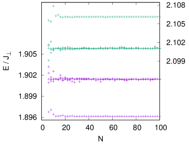
Figure 5: Left(right) y-axis: Two lowest(highest) eigenvalues, i.e., ABS and continuum boundary for each, of two-triplon spectrum versus linear size of $N\times N$ unit-cell system in $(y,z)$-sector of AC-stacking with $J_{\alpha}=-0.1J_{\perp}$ at zero total momentum, $\mathbf{K}=\mathbf{0}$. Finite size effects are negligible beyond $N\gtrsim 15$.

As for the last remaining type of stacking, i.e., AB, we find no clear signatures of ABS at the maximum order of the SE we have generated and for those intralayer couplings acceptable regarding the convergence of the SE. In fact, we have observed weak indications of ABS for this stacking only in limited regions of the BZ and only for $J\gtrsim 1.1$. This we consider unsafe regarding the SE. Interestingly, the absence of ABS for the AB-stacking is consistent with the fact, that local two-triplon eigenstates analogous to Eqs. (4) and (6) cannot be constructed in this case, because two dimers are never coupled by identical Ising exchange from both Kitaev layers.

Finally, we comment on the control of finite size effects in the diagonalization of the $Q=2$ sector of the effective Hamiltonian. The flow of several low- and high-energy eigenstates with system size is shown in Fig. 5. As can be seen, errors due to finite lattice size can be discarded beyond $N\simeq 15$. This is consistent with the strong localization of the ABS. In practice we have employed $N=18$.

IV.3 Anisotropic Kitaev exchange

For anisotropic Kitaev exchange, i.e., $J_{\alpha}/J_{\beta}\neq 1$ for $\alpha\neq\beta$ in general, we focus on the AC-stacking at $J_{x}\neq J_{y}=J_{z}$. This case is of interest, as it provides additional insight into the qualitative picture for the occurrence of the ABS provided in the context of Eqs. (4) and (5).

As described in Secs. IV.1 and IV.2, for AC-stacking, the one-triplon hopping is quasi one-dimensional along the $yz$ zigzag ladder and the width of the one-triplon dispersion, as well as that of the two-triplon scattering-state continuum is therefore primarily determined by the size of $J_{y,z}/J_{\perp}$. Moreover, to lowest order, i.e., for $J_{y,z}=0$, the ABS (anti)binding energy is set by $J_{x}$ from Eqs. (4) and (5).

Performing pCUT at $J_{x}\neq J_{y}=J_{z}$ therefore allows to asses the interplay between the binding and the dispersion. This is shown in Fig. 6. First, at fixed $J_{x}$, varying $J_{y,z}$ one can clearly see that, while for $J_{y,z}=0$ the ABS binding is strongest and exactly of the magnitude given in Eq. (5), finite triplon dispersion reduces the splitting of the ABS off from the scattering-state continuum. However, even for $J_{y,z}\gtrsim J_{x}$ some, albeit small (anti)binding energy remains. Similarly, we can fix $J_{y,z}\neq 0$, as in the inset of Fig. 6 and increase $J_{x}$ beyond $J_{y,z}$. This enhances the binding as compared to the dispersion and hence increases the split-off of the ABS from the continuum. In summary, we observe an adiabatic evolution of the ABS versus $J_{x}/J_{y,z}$, which strongly supports the simple physical picture set forth in Eq. (4).

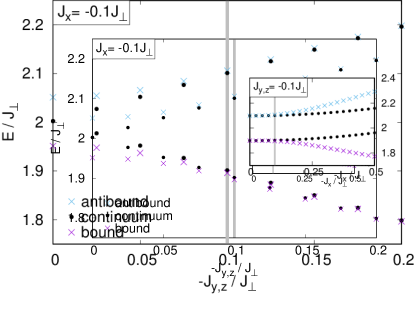
Figure 6: Cyan/magenta crosses: ABS energies and solid dots: upper/lower scattering-state continuum bounds versus $J_{y,z}$ at $J_{y}=J_{z}$ for fixed $J_{x}=-0.1J_{\perp}$ in the $(y,z)$ channel. Gray vertical line: $J_{x}=J_{y}=J_{z}$. Inset: Identical quantities, however versus $J_{x}$ for fixed $J_{y,z}=-0.1J_{\perp}$.

V Raman spectrum

Having discussed the energies of the $Q=1$ and 2 excitations, we now turn to observables. While one-triplon states can be probed by neutrons, Raman scattering is a prime tool to analyze two-triplon excitations in quantum magnets in general [49], including, e.g., paradigmatic frustrated systems [50], Kitaev magnets [51], and dimer magnets [52, 53]. For the latter, Raman scattering will also probe the ABS. Therefore, our focus is on Raman scattering.

The Raman response is obtained from the spectrum of the dynamical correlation function of the Raman operator, encoding the inelastic scattering of light from the system. For local moment systems the latter is mediated by a photon-assisted superexchange process, described by the Loudon-Fleury vertex [54]

$$\mathcal{R}=\sum_{\mathbf{r},\alpha,L}S^{\alpha}_{\mathbf{r},L}S^{\alpha}_{\mathbf{r}+\bm{\delta}_{\alpha}^{L},L}\left[\mathbf{A}^{i}\cdot\bm{\delta}_{\alpha}^{L}\right]\left[\mathbf{A}^{o}\cdot\bm{\delta}_{\alpha}^{L}\right]$$ (7)

where $\mathbf{A}^{i,o}$ is the vector potential of the incoming and outgoing light, using radiation gauge, $i\omega\mathbf{A}={\bf E}$. To simplify, we confine ourselves to a scattering geometry in which the incoming and outgoing polarization of the electric field is in the Kitaev plane. I.e., Eq. (7) has no contributions from the dimer exchange.

From $\mathcal{R}$ and the ground state $\ket{\psi}$, the zero-temperature Raman intensity is given by

$$-\pi I(\omega) ={\rm Im}\bra{\psi}\mathcal{R}^{\dagger}\frac{1}{\omega+i\,0^{+}-H+E_{0}}\mathcal{R}\ket{\psi}$$

$$={\rm Im}\bra{}\mathcal{R}_{\rm eff}^{\dagger}\frac{1}{\omega+i\,0^{+}-H_{\rm eff}+E_{0}}\mathcal{R}_{\rm eff}\ket{}\,,$$ (8)

where the second line refers to the application of the pCUT and, as for $H_{\rm eff}$, the operator $\mathcal{R}_{\rm eff}$ is the pCUT transform of the Raman operator, i.e., $U^{\dagger}\mathcal{R}U$ where $\ket{\psi}=U\ket{}$ by virtue of the pCUT [48, 55]. For the evaluation of $\mathcal{R}_{\rm eff}$, it is important to note, that pCUT provides the generator of the unitary transformation $U$ explicitely.

Since typically, $\mathbf{A}^{i,o}$ refers to light within the visible range, its wave length is exceedingly large compared to the lattice constant. Therefore, the Raman operator Eq. (7) generates excitations of zero total momentum and Raman scattering probes only their spectral density. As a practical consequence, only ${\bf K}=0$ sectors of $H_{\rm eff}$ are relevant for $I(\omega)$.

While $H_{\rm eff}$ is $Q$-diagonal, $\mathcal{R}_{\rm eff}$ in general is not. Therefore $I(\omega)$ constitutes a sum over spectra from subspaces of various triplon numbers. We confine ourselves to the contribution comprising the smallest number of triplons which occurs, namely $Q=2$. While this corresponds to the number of triplons created also by $\mathcal{R}$ itself, the $Q=2$ creation by $\mathcal{R}_{\rm eff}$ involves an operator of very different real-space extent than $\mathcal{R}$.

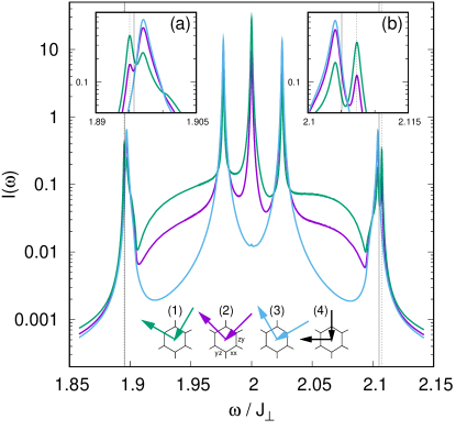
Figure 7: Raman intensity $I(\omega)$ in $(x,x),(y,y),(z,z)$-sector of AC-stacking at $J=-0.1J_{\perp}$ (see Fig. 4) versus energy transfer $\omega$ for three distinct in-plane, perpendicularly polarized, scattering geometries, shown by hexagons (1), (2) and (3). Due to the symmetry of the model $I(\omega)$ is identical for geometries (1) and (4). Letters $\alpha\beta$ on hexagon bonds label upper/lower layer $J_{\alpha/\beta}$ exchange. Dashed(solid) vertical lines: ABS(continuum boundary) energies. Insets (a) and (b): Blow up of intensity in vicinity of ABS.

Based on these preliminaries, we evaluate $I(\omega)$ by continued fraction expansion, using a Lanczos procedure for $H_{\rm eff}$ with the two-triplon states generated by $\mathcal{R}_{\rm eff}\ket{}$ as the start vector. Details can be found in appendix C and in Ref. [47].

Fig. 7 shows the Raman intensity in the AC-stacking for isotropic Kitaev exchange $J_{x,y,z}=J$ calculated with one-triplon matrix elements to $O(9)$, two-triplon interactions to $O(8)$ and $\mathcal{R}_{\rm eff}\ket{}$ to $O(4)$. The imaginary shift off the real $\omega$-axis has been chosen small enough to resolve all intrinsic fine structure of the spectrum. For the truncation order of the continued fraction chosen, this implies some insignificant ripple, visible on the spectrum. For the scattering geometry we have chosen perpendicular polarization of the incoming and outgoing light, varying the angle relative to the tricoordinated nearest-neighbor bonds. Several points can be made. First, the spectrum displays up to five peaks, two of which, namely those on the edges of the continuum are down by approximately one order of magnitude in intensity. Second, the global shape of the intensity is strongly dependent on the scattering angle. In particular, the central peak at $\omega=2$ and the contribution from the ABS - to be discussed shortly - can be suppressed completely for incoming polarization parallel to the stacked $S^{x}S^{x}$-bonds. In this configuration the Raman operator can only directly create $y$- and $z$-triplons, thus suppressing the formation of ABS as depicted in Fig. 4. Third, symmetry properties of the underlying bilayer lattice are respected by $I(\omega)$ as the response is identical for the two symmetry related scattering geometries (1) and (4).

Triplet interactions have a strong impact on the Raman intensity. This can be seen by contrasting $I(\omega)$ from Fig. 7 against $I^{0}(\omega)$ from Fig. 8. In the latter the irreducible two-triplon entries of $H_{\rm eff}$ have been turned off. As is obvious, two of the five peaks in $I(\omega)$ are absent from $I^{0}(\omega)$, and two are strongly suppressed, implying that all of the former are direct consequences of two-triplon interactions. Moreover, the variation with polarization angle is markedly different. In particular no suppression of the central peak occurs, as for $I(\omega)$.

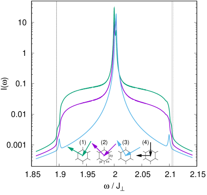
Figure 8: Raman intensity $I^{0}(\omega)$ without two-triplon interactions in $(x,x),(y,y),(z,z)$-sector of AC-stacking at $J=-0.1J_{\perp}$ versus energy transfer $\omega$ for three distinct in-plane, perpendicularly polarized, scattering geometries, shown by hexagons (1), (2) and (3). Due to the symmetry of the model $I^{0}(\omega)$ is identical for geometries (1) and (4). Letters $\alpha\beta$ on hexagon bonds label upper/lower layer $J_{\alpha/\beta}$ exchange. Dashed(solid) vertical lines: ABS(continuum boundary) energies.

Regarding the ABS, Raman scattering on the KHBM turns out to behave very different from conventional $SU(2)$ bilayer spin-systems. In fact, the most prominent ABS, i.e., those from the $(y,z)$ sector remain hidden from light scattering. This is because the Raman operator Eq. (7) will not create two-triplon states of this spin character. Instead, $\mathcal{R}$ can address only states from the $(x,x),(y,y),(z,z)$-sector, which, as discussed in Sec. IV.2, are split-off from the continuum only very weakly. This can be seen both, in the bound and antibound energy range of Fig. 7. Here the Raman intensity displays a fine structure of two peaks. One of them corresponds to the upper edge of the continuum, the other one refers to the ABS. This would certainly pose a challenge to experimental observation of such states. Remarkably, occurrence of the ABS in the Raman spectrum depends on the scattering geometry. This can be seen in Fig. 7, with configuration (3) not displaying ABS.

VI Conclusion

To summarize, using series expansion in terms of the perturbative Continuous Unitary Transformation, we have investigated the elementary excitations of the Kitaev-Heisenberg bilayer magnet in its quantum-dimer phase, with a particular focus on the two-triplon spectrum. In contrast to conventional, $SU(2)$-invariant bilayer quantum-magnets, we have shown the Kitaev-Heisenberg bilayer to display a diverse structure of elementary excitations, depending on two aspects, i.e., the stackings of the bilayer and the triplon components.

Displaying evidence from two sources, i.e., the spectrum and the wave functions, we have disclosed several collective (anti)bound two-triplon states. In principle, we find them to exist for all stackings, however not for all combinations of triplon components. Moreover, for the two-triplon (anti)binding energies, we observe a strong variation versus the type of stacking, with the most prominent (anti)bound states to occur in the AC-stacking. For some of the (anti)bound states we have provided a simple, low-order local picture, involving NN-intralayer Kitaev exchange-links, to explain the (anti)binding of two triplons. This picture is corroborated by our pCUT calculations, using anisotropic exchange couplings.

For an observable probe of our results, we have calculated the magnetic Raman response, resulting from a Loudon-Fleury scattering off the Kitaev planes. We found the Raman intensity to be strongly modified by the two-triplon interactions. In addition to that, we have identified Raman-signatures of (anti)bound states close to the continuum. However, unfortunately, the Raman operator exhibits a selection rule which forbids scattering from the most prominent of the (anti)bound states. Finally we have shown the global shape of the Raman intensity to be very sensitive to the scattering geometry.

Appendix A pCUT-spectra for the KHBM

In this appendix we clarify some details specific to the application of the pCUT to the KHBM. A general description of the method is provided in Ref. [46]. The main idea is to block-diagonalize the Hamiltonian into an effective Hamiltonian $H_{\mathrm{eff}}$. Each block encodes mixing of states corresponding to only a particular number $Q$ of excitation quanta, i.e., $[H_{\text{eff}},H_{0}]=0$. Each block can be treated separately.

The interacting groundstate energy can be extracted from the $Q=0$ block. For the KHBM the unperturbed groundstate is a unique singlet product state, i.e., the $Q=0$ block has size $1\times 1$ and the groundstate energy can be read off directly from the single matrix element obtained by pCUT.

The one-triplon dispersion results from diagonalizing the $Q=1$ block. Due to translational invariance of the Hamiltonian, the first step of this follows from Fourier transformation, which yields a momentum dependent $6\times 6$ matrix ${\bf E}_{\mathbf{k},jl,\alpha\beta}=\sum_{\bf r}e^{i\bm{\rho}_{j}\cdot{\bf k}}\langle\bm{\rho}_{j}\alpha|H_{\rm eff}|{\bf 0}_{l}\beta\rangle-\delta_{\bm{\rho}_{j}{\bf 0}_{l}}\delta_{\alpha\beta}E_{0}^{\text{cl}}$ with $\bm{\rho}_{j=1,2}=(\mathbf{r},\mathbf{r}+\bm{\delta}^{1}_{x}),\alpha,\beta=x,y,z$ and $E_{0}^{\text{cl}}$ evaluated on the same cluster geometry as the corresponding $\langle{\bf 0}_{l}\alpha|H_{\rm eff}|{\bf 0}_{l}\alpha\rangle$ to obtain the irreducible one-triplon matrix element. The generation of clusters is clarified in App. B.

The preceding $6\times 6$ matrix splits into three $2\times 2$ matrices, because the effective Hamiltonian $H_{\text{eff}}$ conserves the parity $P_{\alpha}$ of the number of each triplon component $\alpha=x,y,z$, i.e.,

$$P_{\alpha}=e^{i\pi\sum_{\bm{\rho}_{j}}\hat{n}_{\bm{\rho}_{j}}^{\alpha}}\,.$$ (9)

Here $\hat{n}_{\bm{\rho}_{j}}^{\alpha}$ is the triplon number of triplon $\alpha$ on site $\bm{\rho}_{j}$. All $3\cdot 2$ triplon-dispersions $E_{1,2}^{\alpha}(\mathbf{k})$ can therefore be obtained analytically, and are described in the main text and in Ref. [13].

To proof the parity conservation, one has to analyze the effective spin exchange within pCUT. This can be achieved conveniently by using the singlet-triplon basis as in Eq. (2) and expressing the spin-components via singlet and triplon bond operators [56]

$$S_{\bm{\rho}_{j},L}^{\alpha}=\pm t_{\bm{\rho}_{j}}^{\alpha\,\dagger}s_{\bm{\rho}_{j}}^{\phantom{\dagger}}\pm s_{\bm{\rho}_{j}}^{\dagger}t_{\bm{\rho}_{j}}^{\alpha}-i\epsilon_{\alpha\beta\gamma}t_{\bm{\rho}_{j}}^{\beta\,\dagger}t_{\bm{\rho}_{j}}^{\gamma}$$ (10)

where $\alpha=x,y,z$ is the spin-component, $+(-)$ refers to layer $L=1(2)$, and $t_{\bm{\rho}_{j}}^{\alpha\,(\dagger)}$ ($s_{\bm{\rho}_{j}}^{(\dagger)}$) creates (annihilates) $\alpha$-triplons (singlets) on the interlayer-dimer at site $\bm{\rho}_{j}$. These operators fulfill bosonic commutator relations and need to satisfy the constraint

$$s_{\bm{\rho}_{j}}^{\dagger}s_{\bm{\rho}_{j}}^{\phantom{\dagger}}+t_{\bm{\rho}_{j}}^{\alpha\,\dagger}t_{\bm{\rho}_{j}}^{\alpha\,}=1$$ (11)

to suppress nonphysical states. The Kitaev reads

$$S_{\bm{\rho}_{j},L}^{\alpha}S_{\bm{\rho}^{\prime}_{j^{\prime}},L}^{\alpha}=\sum_{n=-2}^{+2}T^{n}_{\bm{\rho}_{j},\bm{\rho}^{\prime}_{j^{\prime}},L,\alpha}$$ (12)

where $\bm{\rho}^{(\prime)}_{j^{(\prime)}}$ are NN sites on layer $L$, and the ladder operators $T^{n}_{\bm{\rho}_{j},\bm{\rho}^{\prime}_{j^{\prime}},L,\alpha}$ non-locally (in)decrement the number of triplons by $n$ at sites $\bm{\rho}^{(\prime)}_{j^{(\prime)}}$, i.e.,

$$T^{0}_{\bm{\rho}_{j},\bm{\rho}^{\prime}_{j^{\prime}},L,\alpha} =s_{\bm{\rho}_{j}}^{\dagger}t_{\bm{\rho}^{\prime}_{j^{\prime}}}^{\alpha\,\dagger}t_{\bm{\rho}_{j}}^{\alpha}s_{\bm{\rho}^{\prime}_{j^{\prime}}}^{\phantom{\dagger}}+t_{\bm{\rho}_{j}}^{\alpha\,\dagger}s_{\bm{\rho}^{\prime}_{j^{\prime}}}^{\dagger}s_{\bm{\rho}_{j}}^{\phantom{\dagger}}t_{\bm{\rho}^{\prime}_{j^{\prime}}}^{\alpha}$$ (13)

$$\phantom{=}+(\epsilon_{\alpha\beta\gamma})^{2}\left(t_{\bm{\rho}_{j}}^{\beta\,\dagger}t_{\bm{\rho}^{\prime}_{j^{\prime}}}^{\gamma\,\dagger}t_{\bm{\rho}_{j}}^{\gamma}t_{\bm{\rho}^{\prime}_{j^{\prime}}}^{\beta}-t_{\bm{\rho}_{j}}^{\beta\,\dagger}t_{\bm{\rho}^{\prime}_{j^{\prime}}}^{\beta\,\dagger}t_{\bm{\rho}_{j}}^{\gamma}t_{\bm{\rho}^{\prime}_{j^{\prime}}}^{\gamma}\right)\,,$$

$$T^{+1}_{\bm{\rho}_{j},\bm{\rho}^{\prime}_{j^{\prime}},L,\alpha} =\mp i\epsilon_{\alpha\beta\gamma}\left(t_{\bm{\rho}_{j}}^{\alpha\,\dagger}t_{\bm{\rho}^{\prime}_{j^{\prime}}}^{\beta\,\dagger}s_{\bm{\rho}_{j}}^{\phantom{\dagger}}t_{\bm{\rho}^{\prime}_{j^{\prime}}}^{\gamma}+t_{\bm{\rho}_{j}}^{\beta\,\dagger}t_{\bm{\rho}^{\prime}_{j^{\prime}}}^{\alpha\,\dagger}t_{\bm{\rho}_{j}}^{\gamma}s_{\bm{\rho}^{\prime}_{j^{\prime}}}^{\phantom{\dagger}}\right)$$

$$=(T^{-1}_{\bm{\rho}_{j},\bm{\rho}^{\prime}_{j^{\prime}},L,\alpha})^{\dagger}\,,$$ (14)

$$T^{+2}_{\bm{\rho}_{j},\bm{\rho}^{\prime}_{j^{\prime}},L,\alpha} =t_{\bm{\rho}_{j}}^{\alpha\,\dagger}t_{\bm{\rho}^{\prime}_{j^{\prime}}}^{\alpha\,\dagger}s_{\bm{\rho}_{j}}^{\phantom{\dagger}}s_{\bm{\rho}^{\prime}_{j^{\prime}}}^{\phantom{\dagger}}=(T^{-2}_{\bm{\rho}_{j},\bm{\rho}^{\prime}_{j^{\prime}},L,\alpha})^{\dagger}\ .$$ (15)

The ladder operators satisfy $[T^{n}_{\bm{\rho}_{j},\bm{\rho}^{\prime}_{j^{\prime}},L,\alpha},H_{0}]=n\,T^{n}_{\bm{\rho}_{j},\bm{\rho}^{\prime}_{j^{\prime}},L,\alpha}$ and $[T^{n}_{\bm{\rho}_{j},\bm{\rho}^{\prime}_{j^{\prime}},L,\alpha},P_{\beta}]=0$ for $n=0,\pm 2$, as well as $\{T^{n}_{\bm{\rho}_{j},\bm{\rho}^{\prime}_{j^{\prime}},L,\alpha},P_{\beta}\}=0$ for $n=\pm 1$.

Now, turning to Eq. (3), each $C_{l,m,n}$, at $O(k=l{+}m{+}n)$ of the pCUT series for the effective Hamiltonian comprises a real numbered weight from the flow equations [46] and an operator

$$T(\{n_{i}\})=\prod_{i=1}^{k}T^{n_{i}}_{\bm{\rho}_{j_{i}},\bm{\rho}^{\prime}_{j^{\prime}_{i}},L_{i},\alpha_{i}}$$ (16)

with $n_{i}\in\{-2,-1,0,+1,+2\}$. $Q$-conservation implies $\sum_{i=1}^{k}n_{i}=0$ and therefore each $T(\{n_{i}\})$ may contain only an even number of $n_{i}=\pm 1$ ladder operators. In turn $[T(\{n_{i}\}),P_{\alpha}]=0$ for all $T(\{n_{i}\})$. This proves the parity conservation of the pCUT.

$\left(\includegraphics[valign={c},width=65.04034pt]{fig9.pdf}\right)$

Figure 9: Visualization of the structure of the $Q=2$ block of the Hamiltonian (1) for some fixed total momentum $\mathbf{K}$. When ordered by the relative two-triplon distance $|\mathbf{d}|$, the two-triplon interactions $H_{2}$, limited to finite distances by the order of the pCUT expansion, form a block in the upper left and the single triplon propagation $H_{1}$ forms a semi-infinite tail of the matrix.

The two-triplon spectrum is obtained from the $Q=2$ block. States in this block are denoted by $\ket{\bm{\rho}_{j},\bm{\rho}_{j}+\bm{\tau}_{l},\alpha\beta}$ where $\bm{\rho}_{j}$ and $\bm{\rho}_{j}+\bm{\tau}_{l}\neq\bm{\rho}_{j}$ are two distinct sites of the lattice and $\alpha,\beta$ mark the two-triplon components which are present on the dimers. To avoid double counting, we introduce an “ordering”. For that, we choose to have the first triplon located to the lower left of the second triplon and write “$\bm{\rho}_{j}<\bm{\rho}_{j}+\bm{\tau}_{l}$”. The matrix elements of the two-triplon irreducible Hamiltonian $H_{2}$, i.e., that by virtue of which both triplons in the $Q=2$ sector move, are obtained by subtracting off the two-triplon reducible contributions from the matrix elements of $H_{\text{eff}}$, which decomposes into $H_{2}+H_{1}+H_{0}$, where $H_{1(0)}$ move at most $1(0)$ triplons [47], i.e.,

$$\bra{\tilde{\bm{\rho}}^{\phantom{\prime}}_{\tilde{j}},\tilde{\bm{\rho}}^{\prime}_{\tilde{j}},\alpha\beta}H_{2}\ket{\bm{\rho}^{\phantom{\prime}}_{j},\bm{\rho}^{\prime}_{j^{\prime}},\alpha^{\prime}\beta^{\prime}}=$$ (17)

$$\bra{\tilde{\bm{\rho}}^{\phantom{\prime}}_{\tilde{j}},\tilde{\bm{\rho}}^{\prime}_{\tilde{j}},\alpha\beta}H_{\text{eff}}-H_{1}-H_{0}\ket{\bm{\rho}^{\phantom{\prime}}_{j},\bm{\rho}^{\prime}_{j^{\prime}},\alpha^{\prime}\beta^{\prime}}=$$

$$\phantom{-}a^{cl}_{\tilde{\bm{\rho}}^{\phantom{\prime}}_{\tilde{j}},\tilde{\bm{\rho}}^{\prime}_{\tilde{j}},\alpha\beta,\bm{\rho}^{\phantom{\prime}}_{j},\bm{\rho}^{\prime}_{j^{\prime}}\alpha^{\prime}\beta^{\prime}}-E_{0}^{\text{cl}}\delta_{\bm{\rho}^{\phantom{\prime}}_{j},\tilde{\bm{\rho}}^{\phantom{\prime}}_{\tilde{j}}}\delta_{\bm{\rho}^{\prime}_{j^{\prime}},\tilde{\bm{\rho}}^{\prime}_{\tilde{j}}}\delta_{\alpha\alpha^{\prime}}\delta_{\beta\beta^{\prime}}$$

$$-t^{\text{cl}}_{\bm{\rho}^{\phantom{\prime}}_{j},\tilde{\bm{\rho}}^{\phantom{\prime}}_{\tilde{j}},\alpha}\delta_{\bm{\rho}^{\prime}_{j^{\prime}},\tilde{\bm{\rho}}^{\prime}_{\tilde{j}}}\delta_{\alpha\alpha^{\prime}}\delta_{\beta\beta^{\prime}}-t^{\text{cl}}_{\bm{\rho}^{\prime}_{j^{\prime}},\tilde{\bm{\rho}}^{\prime}_{\tilde{j}},\beta}\delta_{\bm{\rho}^{\phantom{\prime}}_{j},\tilde{\bm{\rho}}^{\phantom{\prime}}_{\tilde{j}}}\delta_{\alpha\alpha^{\prime}}\delta_{\beta\beta^{\prime}}$$

$$-t^{\text{cl}}_{\bm{\rho}^{\phantom{\prime}}_{j},\tilde{\bm{\rho}}^{\prime}_{\tilde{j}},\alpha}\delta_{\bm{\rho}^{\prime}_{j^{\prime}},\tilde{\bm{\rho}}^{\phantom{\prime}}_{\tilde{j}}}\delta_{\alpha\beta^{\prime}}\delta_{\beta\alpha^{\prime}}-t^{\text{cl}}_{\bm{\rho}^{\prime}_{j^{\prime}},\tilde{\bm{\rho}}^{\phantom{\prime}}_{\tilde{j}},\beta}\delta_{\bm{\rho}^{\phantom{\prime}}_{j},\tilde{\bm{\rho}}^{\prime}_{\tilde{j}}}\delta_{\alpha\beta^{\prime}}\delta_{\beta\alpha^{\prime}}\,,\hphantom{aa}$$

where $a^{cl}_{\tilde{\bm{\rho}}^{\phantom{\prime}}_{\tilde{j}},\tilde{\bm{\rho}}^{\prime}_{\tilde{j}},\alpha\beta,\bm{\rho}^{\phantom{\prime}}_{j},\bm{\rho}^{\prime}_{j^{\prime}}\alpha^{\prime}\beta^{\prime}}$ is the reducible matrix element of $H_{\text{eff}}$ from pCUT, $t^{\text{cl}}_{\bm{\rho}^{\phantom{\prime}}_{j},\tilde{\bm{\rho}}^{\phantom{\prime}}_{\tilde{j}},\alpha}$ are the irreducible one-triplon contributions, $E_{0}^{\text{cl}}$ is the groundstate energy, and the superscript $cl$ implies that all of the latter have to be evaluated on the same cluster.

We obtain the two-triplon energies by evaluating the spectrum of $H_{\text{eff}}-H_{0}=H_{1}+H_{2}$. This can be achieved in two steps. First, we switch to center of mass and relative coordinates, $\mathbf{R}=\bm{\rho}_{j}+\frac{\bm{\tau}_{l}}{2}$ and $\mathbf{d}=\bm{\tau}_{l}$, respectively, and introduce the Fourier transform with respect to $\mathbf{R}$, i.e.,

$$\ket{\mathbf{K},\mathbf{d},\alpha\beta}=\sum_{\mathbf{R},\mathbf{d}}e^{-i\mathbf{K}\cdot\mathbf{R}}\ket{\mathbf{R}{-}\mathbf{d}/2,\mathbf{R}{+}\mathbf{d}/2,\alpha\beta}\,.$$ (18)

The states $\ket{\mathbf{K},\mathbf{d},\alpha\beta}$ pre-diagonalizes the $Q=2$ block in terms of the total two-triplon momentum $\mathbf{K}$.

For the remaining diagonalization of $H_{1}+H_{2}$ with respect to the relative coordinate $\mathbf{d}$, it is instructive to visualize the structure of the $Q=2$ block at fixed $\mathbf{K}$, shown in Fig. 9. It consists of two types of entries obtained from pCUT. First, a block of irreducible two-triplon interactions $H_{2}$. The rank of this, i.e., the range of the interaction, is not only related to the order of the pCUT, but the absolute size of its matrix elements versus ${\bf d}$ also encodes the physical range and spacial structure of the effective two-triplon interactions. Second, the block displays a semi-infinite banded tail, encoding the scattering states with no mutual interactions, created by $H_{1}$. If $H_{2}$ is set to zero, the remaining $H_{1}$ can be diagonalized analytically by a second Fourier transform with respect to ${\bf d}$, yielding a bare two-triplon spectrum $E_{i}^{\alpha}(\mathbf{k})+E_{j}^{\beta}(\mathbf{k}^{\prime})$ such that $\mathbf{K}=\mathbf{k}+\mathbf{k}^{\prime}$ and $i,j=1,2$.

If $H_{2}$ is finite, it is not possible to analytically diagonalize the matrix - even though all of its entries are analytic expressions, derived from the pCUT. Instead the two-triplon scattering problem at hand is diagonalized numerically, choosing a lattice of linear dimension $\hat{d}$, large enough to contain all of $H_{2}$ at a given order of the pCUT and scattering states up to a distance large enough, to reduce finite size effects sufficiently. As shown in Fig. 5, we find that at $O(8)$, a $\hat{d}\simeq 8$ is sufficient, both, for a faithful representation of the two-triplon continuum and the ABS.

As a final simplification, parity conservation for triplon numbers, Eq. (9), also applies in the $Q=2$ block. It splits the $H_{1}+H_{2}$ matrix into four subblocks which can be diagonalized independently. These are three separate subblocks with triplon components $\{(x,y)\}$, $\{(y,z)\}$ and $\{(z,x)\}$ only, and a fourth block mixing two triplons with components ($\{(x,x)$, $(y,y)$, $(z,z)\}$). In the latter all triplon numbers are of even parity while in the former two triplon numbers have an odd parity.

Appendix B Cluster generation

In this Appendix we describe the generation of clusters on which pCUT matrix elements are evaluated. By virtue of the linked cluster theorem, pCUT hopping matrix elements, in order to be size-consistent, have to be calculated at least on the largest cluster, that is linked through the effective Hamiltonian at a given order $N$ of the series expansion [57, 58]. Since calculation times grow exponentially with cluster size, it is important to generate the clusters such as to include only those lattice sites and bonds which are linked at most.

The cluster generation takes slightly different routes for one-triplon, two-triplon, and Raman operator matrix elements. Each of them is described briefly in the following.

B.1 Cluster for one-triplon matrix elements

A one-triplon matrix element $\langle\bm{\rho}_{j}\alpha|H_{\rm eff}|{\bf 0}_{l}\beta\rangle$ represents the transition amplitude between an initial state $\ket{{\bf 0}_{l}\beta}$ with exactly one triplon at some initial site ${\bf 0}_{l}$ in a singlet-background on all other sites and a final state $\ket{\bm{\rho}_{j}\alpha}$ with the triplon at some final site $\bm{\rho}_{j}$. In the intermediate states of the effective Hamiltonian all triplon flavors mix. Therefore, a classification of the cluster with respect to the latter is not performed.

To generate the cluster for the matrix element $\langle\bm{\rho}_{j}|H_{\rm eff}|{\bf 0}_{l}\rangle$ one has to include all possible paths $P^{k^{\prime},i}_{{\bf 0}_{l},\bm{\rho}_{j}}$ the triplon can take to transit from site ${\bf 0}_{l}$ to site $\bm{\rho}_{j}$, where $0\leq k^{\prime}\leq k$, $k$ is the expansion order and $i$ is an index to enumerate the paths. $P^{k,i}_{{\bf 0}_{l},\bm{\rho}_{j}}$ is a set of site pairs $(\bm{\rho}_{i},\bm{\rho}^{\prime}_{i^{\prime}})$ where each pair encodes a single-order move of the triplon across the lattice. Since the KHBM comprises only NN-exchange, the triplon can, at most, move to an adjacent NN site per order of the pCUT, resulting in $k$ NN-hoppings for a $k$-th order expansion, limiting the cardinality of each $P^{k,i}_{{\bf 0}_{l},\bm{\rho}_{j}}$ strictly to $k$.

All paths $P^{k,i}_{{\bf 0}_{l},\bm{\rho}_{j}}$ up to $k$-th order are obtained iteratively in combination with simultaneous order-by-order calculation of all matrix elements. I.e., by hopping a triplon to NN sites, starting at the final site of a $k$-th order path, $k{+}1$-th order paths are generated

$$P^{k+1,i^{\prime}}_{{\bf 0}_{l},\bm{\rho}^{\prime}_{j^{\prime}}=\bm{\rho}_{j}\pm\delta_{\alpha}^{1}}=P^{k,i}_{{\bf 0}_{l},\bm{\rho}_{j}}\cup\{(\bm{\rho}_{j},\bm{\rho}_{j}\pm\delta_{\alpha}^{1})\}\,.$$ (19)

The index $i^{\prime}$ enumerates the new paths generated. The sign $\pm$ is chosen such that $\bm{\rho}_{j}\pm\delta_{\alpha}^{1}$ is a valid lattice site. See Fig. 10 for an example.

Figure 10: One step in the construction of 1-triplon paths. The second order path $P^{2}_{a,c}=\{(a,b),(b,c)\}$ can be extended to three distinct third order paths $P^{3,1}_{a,d^{\prime}}=\{(a,b),(b,c),(c,d^{\prime})\}$, $P^{3,2}_{a,d^{\prime\prime}}=\{(a,b),(b,c),(c,d^{\prime\prime})\}$ and $P^{3,3}_{a,b}=\{(a,b),(b,c),(c,b)\}$.

From the preceding, the minimal linked cluster $C^{k}_{{\bf 0}_{l},\bm{\rho}_{j}}$, required to calculate a matrix element $\langle\bm{\rho}_{j}|H_{\rm eff}|{\bf 0}_{l}\rangle$ to order $k$ is obtained by combining the sites and bonds of all paths $P^{k^{\prime},i}_{{\bf 0}_{l},\bm{\rho}_{j}}$ connecting the two sites, i.e.,

$$C^{k}_{{\bf 0}_{l},\bm{\rho}_{j}}=\bigcup_{k^{\prime}\leq k,i}P^{k^{\prime},i}_{{\bf 0}_{l},\bm{\rho}_{j}}\ .$$ (20)

For the KHBM we use rotation-symmetries of the lattice to reduce the number of clusters to be generated.

If a cluster $C^{k}_{{\bf 0}_{l},\bm{\rho}^{\prime}_{j}}$ is a subset of another cluster (with identical initial sites), i.e.,

$$C^{k}_{{\bf 0}_{l},\bm{\rho}^{\prime}_{j}}\subset C^{k}_{{\bf 0}_{l},\bm{\rho}_{j}}\ ,$$ (21)

we use a single application of pCUT on the larger cluster $C^{k}_{{\bf 0}_{l},\bm{\rho}_{j}}$ to calculate both matrix elements simultaneously, saving significant computation time.

B.2 Cluster for two-triplon matrix elements

Extending the preceeding, the two-triplon matrix elements $\bra{\tilde{\bm{\rho}}^{\phantom{\prime}}_{\tilde{j}},\tilde{\bm{\rho}}^{\prime}_{\tilde{j}},\alpha\beta}$ $H_{\text{eff}}$ $\ket{\bm{\rho}^{\phantom{\prime}}_{j},\bm{\rho}^{\prime}_{j^{\prime}},\alpha^{\prime}\beta^{\prime}}$ represent transition amplitudes between an initial state $\ket{\bm{\rho}^{\phantom{\prime}}_{j},\bm{\rho}^{\prime}_{j^{\prime}},\alpha^{\prime}\beta^{\prime}}$ with exactly two triplons at initial sites $\bm{\rho}^{\phantom{\prime}}_{j}$ and $\bm{\rho}^{\prime}_{j^{\prime}}$ in a singlet-background on all other sites and a final state $\ket{\tilde{\bm{\rho}}^{\phantom{\prime}}_{\tilde{j}},\tilde{\bm{\rho}}^{\prime}_{\tilde{j}},\alpha\beta}$ with the triplons at final sites $\tilde{\bm{\rho}}^{\phantom{\prime}}_{\tilde{j}}$ and $\tilde{\bm{\rho}}^{\prime}_{\tilde{j}}$. Again, the triplon flavor is not considered.

The generation of clusters for two-triplon matrix elements $\bra{\tilde{\bm{\rho}}^{\phantom{\prime}}_{\tilde{j}},\tilde{\bm{\rho}}^{\prime}_{\tilde{j}}}H_{\text{eff}}\ket{\bm{\rho}^{\phantom{\prime}}_{j},\bm{\rho}^{\prime}_{j^{\prime}}}$ makes use of the one-triplon-paths $P^{k,i}_{{\bf 0}_{l},\bm{\rho}_{j}}$ generated in the previous section. Any linked cluster $P^{k^{\prime\prime},i^{\prime\prime}}_{\bm{\rho}^{\phantom{\prime}}_{j}\bm{\rho}^{\prime}_{j^{\prime}},\tilde{\bm{\rho}}^{\phantom{\prime}}_{\tilde{j}}\tilde{\bm{\rho}}^{\prime}_{\tilde{j}}}$, allowing for two-triplon irreducible interactions comprises two one-triplon paths $P^{k,i}_{\bm{\rho}^{\phantom{\prime}}_{j},\tilde{\bm{\rho}}^{\phantom{\prime}}_{\tilde{j}}}$ and $P^{k^{\prime},i^{\prime}}_{\bm{\rho}^{\prime}_{j^{\prime}},\tilde{\bm{\rho}}^{\prime}_{\tilde{j}}}$, or those with the final sites exchanged, such that the paths have (at least) a common site. See Fig. 11 for an example. I.e.,

$$P^{k^{\prime\prime},i^{\prime\prime}}_{\bm{\rho}^{\phantom{\prime}}_{j}\bm{\rho}^{\prime}_{j^{\prime}},\tilde{\bm{\rho}}^{\phantom{\prime}}_{\tilde{j}}\tilde{\bm{\rho}}^{\prime}_{\tilde{j}}}=P^{k,i}_{\bm{\rho}^{\phantom{\prime}}_{j},\tilde{\bm{\rho}}^{\phantom{\prime}}_{\tilde{j}}}\cup P^{k^{\prime},i^{\prime}}_{\bm{\rho}^{\prime}_{j^{\prime}},\tilde{\bm{\rho}}^{\prime}_{\tilde{j}}}$$ (22)

where $k^{\prime\prime}$ is the order (read number of bonds) of the two-triplon path and $i^{\prime\prime}$ is an appropriate index. By construction the order of the new path has to fulfill $\max(k,k^{\prime})\leq k^{\prime\prime}\leq k+k^{\prime}$.

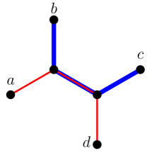
Figure 11: Construction of a two-triplon path: the combination of two third order one-triplon paths $P^{3,i}_{\mathbf{a},\mathbf{d}}$ (red) and $P^{3,i^{\prime}}_{\mathbf{b},\mathbf{c}}$ (blue) result in a fifth order two-triplon-path $P^{5,i^{\prime\prime}}_{\mathbf{a}\mathbf{b},\mathbf{c}\mathbf{d}}$ with one shared bond and two shared sites. This path will be kept for the cluster generation.

Analogous to the one-triplon case the minimal $k$-th order two-triplon linked cluster $C^{k}_{\bm{\rho}^{\phantom{\prime}}_{j}\bm{\rho}^{\prime}_{j^{\prime}},\bm{\rho}^{\phantom{\prime}}_{\tilde{j}}\tilde{\bm{\rho}}^{\prime}_{\tilde{j}}}$ is obtained by combining all two-triplon paths with irreducible two-triplon interactions, i.e.,

$$C^{k}_{\bm{\rho}^{\phantom{\prime}}_{j}\bm{\rho}^{\prime}_{j^{\prime}},\tilde{\bm{\rho}}^{\phantom{\prime}}_{\tilde{j}}\tilde{\bm{\rho}}^{\prime}_{\tilde{j}}}=\bigcup_{k^{\prime\prime}\leq k,i^{\prime\prime}}P^{k^{\prime\prime},i^{\prime\prime}}_{\bm{\rho}^{\phantom{\prime}}_{j}\bm{\rho}^{\prime}_{j^{\prime}},\tilde{\bm{\rho}}^{\phantom{\prime}}_{\tilde{j}}\tilde{\bm{\rho}}^{\prime}_{\tilde{j}}}\ .$$ (23)

B.3 Cluster for two-triplon states generated by $\mathcal{R}_{\rm eff}$

To determine the Raman response, a third type of cluster is needed to evaluate $\mathcal{R}_{\rm eff}\ket{}$ from Eq. (8). As we confine ourselves to the $Q=2$ contribution from $\mathcal{R}_{\rm eff}$ it effectively creates a pair of triplons from the singlet-product state and distributes it across the lattice, generating an effective excitation cloud.

Because the Loudon-Fleury vertex from Eq. (7) is translational invariant and only contains local spin interactions, it is sufficient to treat the Raman operator as acting on a single bond positioned at $({\bf 0},\bm{\delta}_{\alpha})$ only. The clusters are constructed from pseudo two-triplon-paths by combining two one-triplon paths $P^{k,i}_{\bm{\rho}^{\phantom{\prime}}_{j},\tilde{\bm{\rho}}^{\phantom{\prime}}_{\tilde{j}}}$ and $P^{k^{\prime},i^{\prime}}_{\bm{\rho}^{\prime}_{j^{\prime}},\tilde{\bm{\rho}}^{\prime}_{\tilde{j}}}$, requiring that one path must include the first site of the Raman bond and the second one the second site, i.e.,

$${\bf 0}\in P^{k,i}_{\bm{\rho}^{\phantom{\prime}}_{j},\tilde{\bm{\rho}}^{\phantom{\prime}}_{\tilde{j}}}\quad\text{and}\quad\bm{\delta}_{\alpha}\in P^{k^{\prime},i^{\prime}}_{\bm{\rho}^{\prime}_{j^{\prime}},\tilde{\bm{\rho}}^{\prime}_{\tilde{j}}}\ .$$ (24)

Furthermore, in contrast to the two-triplon case, both paths do not need to share a site, as this occurs via the Raman bond. Finally, the two starting sites $\bm{\rho}^{\phantom{\prime}}_{j}$ and $\bm{\rho}^{\prime}_{j^{\prime}}$ need to form a bond included in at least one of both paths or being the Raman bond $({\bf 0},\bm{\delta}_{\alpha})$. The former ensures that the Raman operator can interact with both triplons, the latter mimics the creation of both triplons from the ground state.

The Raman clusters are ultimately formed by combining all valid two-path configurations that lead to the same final positions $\tilde{\bm{\rho}}^{\phantom{\prime}}_{\tilde{j}}$ and $\tilde{\bm{\rho}}^{\prime}_{\tilde{j}}$ regardless of the initial ones.

If, as in the present case, the observable is a sum of operators on different types of bonds, each of them requires generating a separate set of clusters. Their contributions to $\mathcal{R}_{\rm eff}\ket{}$ are additive.

Appendix C Evaluation of the Raman intensity

This appendix explains details for the evaluation of the Raman intensity, i.e., Eq. (8). The Loudon-Fleury vertex, see Eq. (7), can be rewritten as

$$\mathcal{R}=\sum_{\mathbf{r}}\mathcal{R}(\mathbf{r})$$ (25)

with $\mathcal{R}(\mathbf{r})$ acting only on the spins at site $\mathbf{r}$ and its NN-sites. Applying the pCUT yields the effective Raman operator

$$\mathcal{R}_{\text{eff}}=\sum_{\mathbf{r}}\mathcal{R}_{\text{eff}}(\mathbf{r})$$ (26)

with $\mathcal{R}_{\text{eff}}(\mathbf{r})$ now acting on a finite portion of the lattice around the site $\mathbf{r}$, depending on the order of the series expansion. From this we obtain the effective Fourier transformed Raman operator

$$\mathcal{R}_{\text{eff}}(\mathbf{K})=\frac{1}{\sqrt{N}}\sum_{\mathbf{r}}\mathrm{e}^{i\mathbf{K}\mathbf{r}}\mathcal{R}_{\text{eff}}(\mathbf{r})$$ (27)

where $\mathbf{K}$ is the momentum transferred and $N$ is the number of lattice sites.

As mentioned in Sec. V, $\mathcal{R}_{\rm eff}$ is not diagonal in $Q$ and we focus on the lowest number of triplons excited only, i.e., $Q=2$. Thus we confine $\mathcal{R}_{\text{eff}}(\mathbf{r})$ to those parts $\mathcal{R}_{\text{eff},2}(\mathbf{r})$ that excite exactly two triplons from the ground state $\ket{}$. Because $\mathcal{R}_{\text{eff}}(\mathbf{r})$ only acts on a finite region of the lattice the resulting state $\mathcal{R}_{\text{eff},2}(\mathbf{r})\ket{}$ comprises a finite sum of two-triplon states $\ket{\bm{\rho}_{j},\bm{\rho}_{j}+\bm{\tau}_{l},\alpha\beta}$ only. Thus $\mathcal{R}_{\text{eff},2}(\mathbf{K})\ket{}$ will also contain only a finite number of two-triplon states $\ket{\mathbf{K},\bm{\tau}_{l},\alpha\beta}$ of fixed momentum.

This allows to treat the action of $\left[\omega+i\,0^{+}-H_{\text{eff}}+E_{0}\right]^{-1}$ in Eq. (8) by tridiagonalization [47, 59, 60], resulting in a continued fraction expression for the Raman intensity, i.e.,

$$-\pi I(\omega)={\rm Im}\frac{\bra{}\mathcal{R}_{\text{eff},2}^{\dagger}(\mathbf{K})\mathcal{R}_{\text{eff},2}(\mathbf{K})\ket{}}{\omega-a_{0}-\frac{b_{1}^{2}}{\omega-a_{1}-\frac{b_{2}^{2}}{\omega-\dots}}}\ .$$ (28)

The coefficients $a_{n}$, $b_{n}^{2}$ are obtained by iteration

$$\ket{f_{n+1}} =(H_{\text{eff}}-E_{0})\ket{f_{n}}-a_{n}\ket{f_{n}}-b^{2}_{n}\ket{f_{n-1}}$$

$$a_{n} =\frac{\bra{f_{n}}(H_{\text{eff}}-E_{0})\ket{f_{n}}}{\langle f_{n}|f_{n}\rangle}$$

$$b^{2}_{n+1} =\frac{\langle f_{n+1}|f_{n+1}\rangle}{\langle f_{n}|f_{n}\rangle}\,,$$ (29)

starting with $\ket{f_{0}}=\mathcal{R}_{\text{eff},2}(\mathbf{K})\ket{}$.

The action of the effective Hamiltonian can be replaced by $H_{\text{eff}}-E_{0}=H_{1}+H_{2}$, allowing to reuse matrix elements for propagating the states $\ket{f_{n}}$, which have been calculated previously for the one- and two-triplon spectra (see appendix A). Because the iteration only requires to save the last three states, the calculation is very memory efficient and limited only by the computation time allotted. We evaluate coefficients up to $n=500$ and truncate the continued fraction at that point by setting $b_{500}=0$.

References

- [1] S. Sachdev, Quantum Magnetism and Criticality, Nature Physics 4, 173 (2008).
- [2] L. Wang, K. S. D. Beach, and A. W. Sandvik, Phys. Rev. B 73, (2006).
- [3] M. Matsumoto, B. Normand, T. M. Rice, and M. Sigrist, Phys. Rev. B 69, (2004).
- [4] R. R. P. Singh and N. Elstner, Phys. Rev. Lett. 81, 4732 (1998).
- [5] R. F. Bishop, P. H. Y. Li, O. Götze, and J. Richter, Phys. Rev. B 100, 024401 (2019).
- [6] S. Miyahara and K. Ueda, Phys. Rev. Lett. 82, 3701 (1999).
- [7] S. E. Sebastian, N. Harrison, C. D. Batista, L. Balicas, M. Jaime, P. A. Sharma, N. Kawashima, and I. R. Fisher, Nature 441, 617 (2006).
- [8] P. Merchant, B. Normand, K. W. Krämer, M. Boehm, D. F. McMorrow, and Ch. Rüegg, Nature Physics 10, 373 (2014).
- [9] M. B. Stone, M. D. Lumsden, S. Chang, E. C. Samulon, C. D. Batista, and I. R. Fisher, Phys. Rev. Lett. 100, 237201 (2008), ibid 105, 169901 (2010).
- [10] R. Melzi, P. Carretta, A. Lascialfari, M. Mambrini, M. Troyer, P. Millet, and F. Mila, Phys. Rev. Lett. 85, 1318 (2000).
- [11] H. Kageyama, K. Yoshimura, R. Stern, N. V. Mushnikov, K. Onizuka, M. Kato, K. Kosuge, C. P. Slichter, T. Goto, and Y. Ueda, Phys. Rev. Lett. 82, 3168 (1999).
- [12] H. Tomishige, J. Nasu, and A. Koga, Phys. Rev. B 97, 094403 (2018).
- [13] U. F. P. Seifert, J. Gritsch, E. Wagner, D. G. Joshi, W. Brenig, M. Vojta, and K. P. Schmidt, Phys. Rev. B 98, 155101 (2018).
- [14] H. Tomishige, J. Nasu, and A. Koga, Phys. Rev. B 99, 174424 (2019).
- [15] A. Koga, H. Tomishige, and J. Nasu, J. Supercond. Nov. Magn. 32, 1827 (2019).
- [16] A. Kitaev, Ann. Phys. (N.Y.) 321, 2 (2006).
- [17] X.-Y. Feng, G.-M. Zhang, and T. Xiang, Phys. Rev. Lett. 98, 087204 (2007).
- [18] H.-D. Chen and Z. Nussinov, J. Phys. A: Math. Theor. 41, 075001 (2008).
- [19] Z. Nussinov and G. Ortiz, Phys. Rev. B 79, 214440 (2009).
- [20] S. Mandal, R. Shankar and G. Baskaran, J. Phys. A: Math. Theor. 45, 335304 (2012).
- [21] G. Jackeli and G. Khaliullin, Phys. Rev. Lett. 102, 017205 (2009).
- [22] J. Chaloupka, G. Jackeli, and G. Khaliullin Phys. Rev. Lett. 105 027204 (2010).
- [23] K. W. Plumb, J. P. Clancy, L. J. Sandilands, V. V. Shankar, Y. F. Hu, K. S. Burch, H.-Y. Kee, and Y.-J. Kim, Phys. Rev. B 90, 041112 (2014).
- [24] A. Banerjee, C. A. Bridges, J.-Q. Yan, A. A. Aczel, L. Li, M. B. Stone, G. E. Granroth, M. D. Lumsden, Y. Yiu, J. Knolle, S. Bhattacharjee, D. L. Kovrizhin, R. Moessner, D. A. Tennant, D. G. Mandrus, and S. E. Nagler, Nature Materials 15, 733 (2016).
- [25] A. Banerjee, J. Yan, J. Knolle, C. A. Bridges, M. B. Stone, M. D. Lumsden, D. G. Mandrus, D. A. Tennant, R. Moessner, and S. E. Nagler, Science 356, 1055 (2017).
- [26] A. Banerjee, P. Lampen-Kelley, J. Knolle, C. Balz, A. A. Aczel, B. Winn, Y. Liu, D. Pajerowski, J. Yan, C. A. Bridges, A. T. Savici, B. C. Chakoumakos, M. D. Lumsden, D. A. Tennant, R. Moessner, D. G. Mandrus, and S. E. Nagler, Npj Quantum Materials 3, 8 (2018).
- [27] S. Trebst, Kitaev Materials, Lecture Notes of the 48th IFF Spring School 2017, S. Blügel, Y. Mokrousov, T. Schäpers, Y. Ando (Eds.), ISBN 978-3-95806-202-3
- [28] S. M. Winter, A. A. Tsirlin, M. Daghofer, J. van den Brink, Y. Singh, P. Gegenwart, and R. Valentí, J. Phys.: Condens. Matter 29, 493002 (2017).
- [29] L.-M. Duan, E. Demler, and M. D. Lukin, Phys. Rev. Lett. 91, 090402 (2003).
- [30] Y. Miura, Y. Yasui, M. Sato, N. Igawa, and K. Kakurai, J. Phys. Soc. Jpn. 76, 033705 (2007).
- [31] S. A. J. Kimber, C. D. Ling, D. J. P. Morris, A. Chemseddine, P. F. Henry, and D. N. Argyriou, J. Mater. Chem. 20, 8021 (2010).
- [32] G. Khaliullin, Phys. Rev. Lett. 111, 197201 (2013).
- [33] J. Chaloupka and G. Khaliullin, Phys. Rev. B 100, 224413 (2019).
- [34] P. S. Anisimov, F. Aust, G. Khaliullin, and M. Daghofer, Phys. Rev. Lett. 122, 177201 (2019).
- [35] Ch. Rüegg, B. Normand, M. Matsumoto, Ch. Niedermayer, A. Furrer, K. W. Krämer, H.-U. Güdel, Ph. Bourges, Y. Sidis, and H. Mutka, Phys. Rev. Lett. 95, 267201 (2005).
- [36] K. W. Plumb, K. Hwang, Y. Qiu, L. W. Harriger, G. E. Granroth, A. I. Kolesnikov, G. J. Shu, F. C. Chou, C. Rüegg, Y. B. Kim, and Y.-J. Kim, Nature Physics 12, 3 (2016).
- [37] J. Romhányi, K. Penc, and R. Ganesh, Nature Communications 6, 1 (2015).
- [38] Ch. Rüegg, B. Normand, M. Matsumoto, A. Furrer, D. F. McMorrow, K. W. Krämer, H.-U. Güdel, S. N. Gvasaliya, H. Mutka, and M. Boehm, Phys. Rev. Lett. 100, 205701 (2008).
- [39] C. Knetter, A. Bühler, E. Müller-Hartmann, and G. S. Uhrig, Phys. Rev. Lett. 85, 3958 (2000).
- [40] A. Collins and C. J. Hamer, Phys. Rev. B 78, 054419 (2008).
- [41] P. A. McClarty, F. Krüger, T. Guidi, S. F. Parker, K. Refson, A. W. Parker, D. Prabhakaran, and R. Coldea, Nature Physics 13, 8 (2017).
- [42] H. Nojiri, H. Kageyama, K. Onizuka, Y. Ueda, and M. Motokawa, J. Phys. Soc. Jpn. 68, 2906 (1999).
- [43] P. Lemmens, M. Grove, M. Fischer, G. Güntherodt, V. N. Kotov, H. Kageyama, K. Onizuka, and Y. Ueda, Phys. Rev. Lett. 85, 2605 (2000).
- [44] N. Aso, H. Kageyama, K. Nukui, M. Nishi, H. Kadowaki, Y. Ueda, and K. Kakurai, J. Phys. Soc. Jpn. 74, 2189 (2005).
- [45] F. Wegner, Ann. Physik 3 (1994) 77-91
- [46] C. Knetter, G.S. Uhrig, Eur. Phys. J. B 13, 209-225 (2000).
- [47] C. Knetter, K.P. Schmidt, G.S. Uhrig, Eur. Phys. J. B 36, 525-544 (2003).
- [48] C. Knetter, Perturbative continuous unitary transformations: spectral properties of low dimensional spin systems, Doctoral dissertation, University of Cologne, 2003.
- [49] P. Lemmens, M. Fischer, M. Grove, P.H.M. v. Loosdrecht, G. Els, E. Sherman, C. Pinettes, and G. Güntherodt, Advances in Solid State Physics Vol. 39 (Vieweg, Braunschweig, 1999).
- [50] N. Perkins and W. Brenig, Phys. Rev. B 77, 174412 (2008).
- [51] D. Wulferding, Y. Choi, S.-H. Do, C. H. Lee, P. Lemmens, C. Faugeras, Y. Gallais, and K.-Y. Choi, Nat. Commun. 11, 1 (2020).
- [52] W. Brenig and K.W. Becker, Phys. Rev. B 64, 214413 (2001).
- [53] C. Jurecka, V. Grützun, A. Friedrich, and W. Brenig, Eur. Phys. J. B 21, 469 (2001).
- [54] P. A. Fleury and R. Loudon, Phys. Rev. 166, 514 (1968).
- [55] C. Knetter, G.S. Uhrig, Phys. Rev. Lett. 92, 027204 (2004).
- [56] S. Sachdev, R. N. Bhatt, Phys. Rev. B 41, 9323 (1990).
- [57] L. P. Kadanoff and M. Kohmoto, J. Phys. A 14, 1291 (1981).
- [58] L. G. Marland, J. Phys. A 14, 2047 (1981).
- [59] C. Lanczos, J. Res. Nat. Bur. Stand. 45, 255 (1950).
- [60] V. S. Viswanath, G. Müller, The Recursion Method Application to Many-Body Dynamics (Springer-Verlag Berlin Heidelberg, 1994).