An alternative reconstruction for WENO schemes with adaptive order

Abstract

We propose an alternative reconstruction for weighted essentially non-oscillatory schemes with adaptive order (WENO-AO) for solving hyperbolic conservation laws. The alternative reconstruction has a more concise form than the original WENO-AO reconstruction. Moreover, it is a strictly convex combination of polynomials with unequal degrees. Numerical examples show that the alternative reconstruction maintains the accuracy and robustness of the WENO-AO schemes.

1 Introduction

The solution to a hyperbolic conservation law commonly contains both discontinuities and smooth regions with sophisticated structures, so numerical schemes with high-order convergence and excellent shock-capturing properties are desired for solving general hyperbolic conservation laws. The essentially non-oscillatory (ENO) schemes and weighted ENO (WENO) schemes are state-of-the-art such schemes and become mainstream in many applications.

The history of ENO schemes can date back to 1980s. Harten and his coworkers [1] constructed uniformly high-order accurate ENO schemes by slightly relaxing the TVD constraint [2]. ENO schemes achieve uniformly high-order accuracy and the non-oscillatory feature by the strategy of choosing the smoothest stencil from several local candidates. Shu and Osher [3, 4] significantly improved the efficiency of ENO schemes by using TVD Runge-Kutta time discretizations and numerical fluxes reconstructions instead of cell average reconstructions. Based on ENO schemes, Liu et al. [5] proposed WENO schemes by assigning proper weights to the local candidate stencils. Jiang and Shu [6] provided a general framework for designing smooth indicators and weights for WENO schemes to achieve the optimal order in smooth regions while maintaining the non-oscillatory feature at discontinuities. Borges et al. [7] further improved the accuracy of WENO schemes by redesigning the nonlinear weights. Besides, many extended ENO/WENO schemes are proposed and a lot of shock capturing high-order schemes were constructed in the light of ENO/WENO ideas, such as the monotonicity preserving WENO schemes [8], the weighted compact nonlinear schemes [9], the compact central WENO schemes [10, 11, 12], the Hermite WENO schemes [13, 14], the WENO-ADER schemes [15, 16, 17], the $P_{N}P_{M}$ schemes [18, 19, 20], and so forth.

Recently, the WENO schemes with adaptive order (WENO-AO) attracted a lot of interest. WENO-AO schemes started from the fifth-order WENO-ZQ scheme [21], and was further developed by Balsara et al. [22]. The building block of WENO-AO schemes is the combination of polynomials with different degrees that was originally proposed by Levy et al. [12]. The main advantage of WENO-AO schemes is that they can adjust their order adaptively depending on the smoothness of the solutions thanks to the building block. Therefore, it is easy to construct numerical schemes with multi-resolution [22, 23, 24, 25, 26]. In the original reconstruction [12, 21, 22], the high-order polynomial needs to subtract the low-order polynomials in order to recover the optimal high-order polynomial in smooth regions. In doing so, the reconstructed polynomial is not a strictly convex combination of the low-order and high-order polynomials. Balsara et al. [22] already realized this issue when constructing the WENO-AO(7,5,3) scheme. Although this slight imperfection seems not to affect the practical behavior, a purist might still seek for a cure. In this note, we propose an alternative reconstruction which ensures the convexity property and maintains the accuracy and efficiency of WENO-AO schemes.

2 A brief review of finite difference WENO-AO schemes

We consider the one-dimensional scalar conservation law,

$$\frac{\partial u}{\partial t}+\frac{\partial f(u)}{\partial x}=0,x\in[x_{L},x_{R}],t\in[0,\infty).$$ (1)

The spatial domain $[x_{L},x_{R}]$ is discretized into uniform intervals by $x_{i}=x_{L}+(i-1)\Delta x$ ($i=1\text{ to }N+1$), where $\Delta x=(x_{R}-x_{L})/N$. The finite difference WENO schemes can be expressed in the following conservative form

$$\frac{du_{i}(t)}{dt}=\mathcal{L}(u_{i}(t))=-\frac{\hat{f}_{i+1/2}-\hat{f}_{i-1/2}}{\Delta x},$$ (2)

where the numerical flux $\hat{f}_{i\pm 1/2}$ approximates the function $h(x)$, that is implicitly defined by $f(u(x))=\frac{1}{\Delta x}\int_{x-\Delta x/2}^{x+\Delta x/2}h(\xi)d\xi$ [3], at $x_{i\pm 1/2}$.

In order to enhance the robustness of the scheme, we usually introduce the upwind mechanism by choosing an upwind-biased stencil according to the direction of the wave propagation, i.e., the sign of $\frac{df(u)}{du}$. For a general flux, the sign of $\frac{df(u)}{du}$ is not constant, but it can be split into two parts as

$$f(u)=f^{+}(u)+f^{-}(u),$$ (3)

where $\frac{df^{+}(u)}{du}\geq 0$ and $\frac{df^{-}(u)}{du}\leq 0$. For example, the global Lax–Friedrichs flux splitting method splits the flux as

$$f^{\pm}(u)=\frac{1}{2}(f(u)\pm\alpha u),$$ (4)

where $\alpha=\mbox{max}\left|\frac{df(u)}{du}\right|$ and the maximum is taken over the whole computational domain.

After the flux splitting, we respectively construct polynomials to approximate $\hat{f}^{\pm}(u)$ on several sub-stencils of an upwind-biased large stencil, and then use a nonlinear function of the stencils’ smoothness indicators to combine the constructed polynomials. Balsara et al. [22] provided an efficient way to construct a polynomial and to calculate the corresponding smoothness indicator on a given stencil by using Legendre basis. In classical WENO reconstructions [6, 7], the sub-stencils have an equal size, and so do the associated polynomials. By carefully design the weights for the sub-stencils, the reconstructed polynomial recovers the optimal high-order polynomial on the large stencil in smooth regions and tends to the low-order polynomial on the smoothest sub-stencil. However, the reconstructed polynomial cannot always recover the optimal high-order polynomial, especially for multidimensional reconstructions. The WENO-AO reconstruction fixes this issue via a non-linear hybridization between the optimal high-order polynomials and low-order polynomials. For example, the WENO-AO(5,3) reconstruction is expressed as [22]

$$\begin{split}P^{\mbox{AO(5,3)}}(x)&=\frac{\bar{w}_{3}^{r5}}{\gamma_{3}^{r5}}\left(P_{3}^{r5}(x)-\gamma_{1}^{r3}P_{1}^{r3}(x)-\gamma_{2}^{r3}P_{2}^{r3}(x)-\gamma_{3}^{r3}P_{3}^{r3}(x)\right)\\ &+\bar{w}_{1}^{r3}P_{1}^{r3}(x)+\bar{w}_{2}^{r3}P_{2}^{r3}(x)+\bar{w}_{3}^{r3}P_{3}^{r3}(x),\end{split}$$ (5)

where $P_{3}^{r5}(x)$ is the optimal fourth-order polynomial, $P_{k}^{r3}(x)$ $(k=1,2,3)$ are second-order polynomials, and $\gamma$ and $\bar{w}$ are corresponding linear and nonlinear weights. The specific forms of the polynomials and the weights can be found in [22]. It is easy to verify that the reconstructed polynomial $P^{\mbox{AO(5,3)}}(x)$ recovers the optimal polynomial $P_{3}^{r5}(x)$ when $\bar{w}_{n}=\gamma_{n}$. Using the above idea, we can construct numerical schemes with multi-resolution [22, 23, 24, 25, 26].

It is straightforward to extend the finite difference WENO schemes to multi-dimensional cases, because the same reconstruction procedure for approximating the numerical fluxes can be implemented in a dimension-by-dimension manner. In order to eliminate spurious oscillations as much as possible, the reconstruction procedure is applied in the characteristic space when solving hyperbolic systems.

As for the time integration, we adopt the method of lines which first approximates the numerical fluxes by WENO reconstructions and uses the third-order TVD Runge-Kutta method [3] to solve the system of ordinary differential equations, i.e., $\frac{du_{i}(t)}{dt}=\mathcal{L}(u_{i}(t))$.

3 An alternative WENO-AO reconstruction

As we can see, the first part on the right hand side of Eq. (5) contains negative coefficients for $P_{k}^{r3}(x)$ $(k=1,2,3)$. Therefore, $P^{\mbox{AO(5,3)}}(x)$ is not a strictly convex combination of $P_{3}^{r5}(x)$ and $P_{k}^{r3}(x)$ $(k=1,2,3)$. In order to fix this defect, we propose an alternative WENO-AO (WENO-AOA) reconstruction. Without loss of generality, the WENO-AOA(5,3) reconstruction can be expressed as

$$P^{\mbox{AOA(5,3)}}(x)=\bar{w}_{3}^{r5}P_{3}^{r5}(x)+\bar{w}_{1}^{r3}P_{1}^{r3}(x)+\bar{w}_{2}^{r3}P_{2}^{r3}(x)+\bar{w}_{3}^{r3}P_{3}^{r3}(x),$$ (6)

where $P_{3}^{r5}(x)$ and $P_{k}^{r3}(x)$ $(k=1,2,3)$ are the same as the original WENO-AO reconstruction. The un-normalized weights are slightly modified from Borges et al. [7]

$$\begin{split}w_{3}^{r5}=\gamma_{3}^{r5}\left[1+\left(\frac{\tau}{\beta_{3}^{r5}+\epsilon}\right)^{2}\right],\quad w_{1}^{r3}=\gamma_{1}^{r3}\left(\frac{\tau}{\beta_{1}^{r3}+\epsilon}\right)^{2},\\ w_{2}^{r3}=\gamma_{2}^{r3}\left(\frac{\tau}{\beta_{2}^{r3}+\epsilon}\right)^{2},\quad w_{3}^{r3}=\gamma_{3}^{r3}\left(\frac{\tau}{\beta_{3}^{r3}+\epsilon}\right)^{2},\end{split}$$ (7)

where $\epsilon=10^{-40}$ is used to avoid singularity, $\gamma$ represents constant linear weights, the smoothness indicator measuring the regularity of a $n$th order polynomial $p_{n}(x)$ on $[x_{i-1/2},x_{i+1/2}]$ is given by [6]

$$\beta_{n}=\sum_{l=1}^{n}\Delta x^{2l-1}\int_{x_{i-1/2}}^{x_{i+1/2}}\left(\frac{d^{l}p_{n}(x)}{dx^{l}}\right)^{2}dx,$$ (8)

and the parameter $\tau$ is defined as

$$\tau=\frac{1}{3}\left(|\beta_{3}^{r5}-\beta_{1}^{r3}|+|\beta_{3}^{r5}-\beta_{2}^{r3}|+|\beta_{3}^{r5}-\beta_{3}^{r3}|\right).$$ (9)

Finally, the normalized weights are given by

$$\begin{split}&\bar{w}_{3}^{r5}=\frac{w_{3}^{r5}}{w_{3}^{r5}+w_{1}^{r3}+w_{2}^{r3}+w_{3}^{r3}},\\ &\bar{w}_{k}^{r3}=\frac{w_{k}^{r3}}{w_{3}^{r5}+w_{1}^{r3}+w_{2}^{r3}+w_{3}^{r3}},\quad(k=1,2,3).\end{split}$$ (10)

The corresponding explicit expressions of the smoothness indicators can be found in [7, 21, 22] and their Taylor series expansions at $x_{i}$ are given as

$$\begin{split}&\beta_{3}^{r5}=f_{i}^{{}^{\prime}2}\Delta x^{2}+\frac{13}{12}f_{i}^{{}^{\prime\prime}2}\Delta x^{4}+O(\Delta x^{6}),\\ &\beta_{1}^{r3}=f_{i}^{{}^{\prime}2}\Delta x^{2}+\left(\frac{13}{12}f_{i}^{{}^{\prime\prime}2}-\frac{2}{3}f^{\prime}_{i}f^{\prime\prime\prime}_{i}\right)\Delta x^{4}-\left(\frac{13}{6}f^{\prime\prime}_{i}f^{\prime\prime\prime}_{i}-\frac{1}{2}f^{\prime}_{i}f^{\prime\prime\prime\prime}_{i}\right)\Delta x^{5}+O(\Delta x^{6}),\\ &\beta_{2}^{r3}=f_{i}^{{}^{\prime}2}\Delta x^{2}+\left(\frac{13}{12}f_{i}^{{}^{\prime\prime}2}+\frac{1}{3}f^{\prime}_{i}f^{\prime\prime\prime}_{i}\right)\Delta x^{4}+O(\Delta x^{6}),\\ &\beta_{3}^{r3}=f_{i}^{{}^{\prime}2}\Delta x^{2}+\left(\frac{13}{12}f_{i}^{{}^{\prime\prime}2}-\frac{2}{3}f^{\prime}_{i}f^{\prime\prime\prime}_{i}\right)\Delta x^{4}+\left(\frac{13}{6}f^{\prime\prime}_{i}f^{\prime\prime\prime}_{i}-\frac{1}{2}f^{\prime}_{i}f^{\prime\prime\prime\prime}_{i}\right)\Delta x^{5}+O(\Delta x^{6}).\end{split}$$ (11)

For smooth solutions, it is easy to verify that

$$\bar{w}_{k}^{r3}\propto\begin{cases}O\left(\Delta x^{4}\right),&\mbox{if }f^{\prime}_{i}\neq 0,f^{\prime\prime\prime}_{i}\neq 0\\ O\left(\Delta x^{2}\right),&\mbox{if }f^{\prime}_{i}=0,f^{\prime\prime}_{i}\neq 0,f^{\prime\prime\prime}_{i}\neq 0.\end{cases}\quad(k=1,2,3).$$ (12)

Since $\bar{w}_{3}^{r5}+\sum_{k=1}^{3}\bar{w}_{k}^{r3}=1$, the difference between the limited polynomial and the optimal high-order polynomial can be written as

$$\varepsilon=P^{\mbox{AOA(5,3)}}(x)-P_{3}^{r5}(x)=\sum_{k=1}^{3}\bar{w}_{k}^{r3}\left(P_{k}^{r3}(x)-P_{3}^{r5}(x)\right).$$ (13)

Because $P_{3}^{r5}(x)$ is a fifth-order approximation and $P_{k}^{r3}(x)$ $k=1,2,3$ are third-order approximations, we have $P_{k}^{r3}(x)-P_{3}^{r5}(x)\propto\Delta x^{3}$. Combining Eqs. (12) and (13), we obtain

$$\varepsilon\propto\begin{cases}O\left(\Delta x^{7}\right),&\mbox{if }f^{\prime}_{i}\neq 0,f^{\prime\prime\prime}_{i}\neq 0\\ O\left(\Delta x^{5}\right),&\mbox{if }f^{\prime}_{i}=0,f^{\prime\prime}_{i}\neq 0,f^{\prime\prime\prime}_{i}\neq 0.\end{cases}\quad(k=1,2,3).$$ (14)

That is to say, $P^{\mbox{AOA(5,3)}}(x)$ does not violate the order of the optimal high-order polynomial $P_{3}^{r5}(x)$ in smooth regions including at local first-order extrema.

When the large stencil contains discontinuities, we have $\tau\propto O\left(1\right)$, and $\beta_{3}^{r5}\propto O\left(1\right)$. However, one of the low-order polynomial $P_{k}^{r3}(x)$ ($k$=1,2,3) is still smooth, and we have $\beta_{k}^{r3}\propto O\left(\Delta x^{2}\right)$ ($k$=1 or 2 or 3). Therefore, $\bar{w}_{3}^{r5}$ becomes very small, and $P^{\mbox{AOA(5,3)}}(x)$ approaches to the smooth low-order polynomial. This property makes the reconstruction non-oscillatory at discontinuities.

Remark 1.

Comparing Eq. (6) with Eq. (5), the proposed WENO-AOA reconstruction has a more concise form than the original WENO-AO reconstruction. More importantly, WENO-AOA reconstruction provided a strictly convex combination of polynomials with unequal degrees.

4 Numerical examples

As suggested by Balsara et al. [22], we set the linear weights $\gamma_{3}^{r5}=\gamma_{Hi}$, $\gamma_{1}^{r3}=\gamma_{3}^{r3}=0.5(1-\gamma_{Hi})(1-\gamma_{Lo})$, $\gamma_{2}^{r3}=(1-\gamma_{Hi})\gamma_{Lo}$, where $\gamma_{Hi}=\gamma_{Lo}=0.85$. Without further illustration, we set CFL=0.5 for all cases.

4.1 Linear advection

	WENO-AO(5,3)				WENO-AOA(5,3)
Mesh size	$L_{1}$	Order	$L_{\infty}$	Order	$L_{1}$	Order	$L_{\infty}$	Order
1/25	2.11E-6	-	3.38E-6	-	2.57E-6	-	4.11E-6	-
1/50	6.67E-8	4.98	1.06E-7	4.99	8.11E-8	4.99	1.29E-7	4.99
1/100	2.09E-9	5.00	3.31E-9	5.00	2.54E-9	5.00	4.02E-9	5.00
1/200	6.66E-11	4.97	1.05E-10	4.98	8.02E-11	4.99	1.26E-10	5.00

Table 1: Numerical errors of the advection of the sinusoidal wave at $t=2$ computed by WENO-AO(5,3) and WENO-AOA(5,3) with different mesh sizes.

We solve the scalar linear advection equation $\frac{\partial u}{\partial t}+\frac{\partial u}{\partial x}=0$ on the computational domain [-1, 1] with periodic boundaries. The first case is the advection of the sinusoidal wave $u(x,0)=sin(\pi x)$. Since the order of the time discretization does not match with the order of the space discretization, we set $\Delta t=\Delta x^{5/3}$ to test the convergence rate of the numerical solutions. Table 1 shows the average error $L_{1}$ and the maximum error $L_{\infty}$ at $t=2$ on different meshes induced by WENO-AO(5,3) and WENO-AOA(5,3). We observe that the numerical errors of WENO-AO(5,3) and WENO-AOA(5,3) are quite close, and both schemes achieve the optimal fifth-order convergence rate.

(a) WENO-AO(5,3)

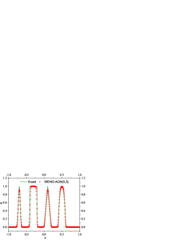
(b) WENO-AOA(5,3)

Figure 1: The advection of a combination of Gaussians, a square wave, a sharp triangle wave, and a half ellipse arranged from left to right at $t=20$ calculated by WENO-AO(5,3) and WENO-AOA(5,3) with 401 mesh points.

The second case is the advection of a combination of Gaussians, a square wave, a sharp triangle wave, and a half ellipse arranged from left to right. This case was first proposed by Jiang and Shu [6], and the specific settings can be found therein. The simulations are performed by using 401 mesh points and terminate at $t=20$. Fig. 1 shows the profiles of $u$ calculated by WENO-AO(5,3) and WENO-AOA(5,3). We observe that the two schemes perform similarly for all kinds of solutions.

5 Double Mach reflection problem

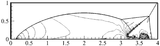
(a) WENO-AO(5,3)

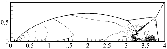
(b) WENO-AOA(5,3)

Figure 2: The entire view of the density contours of double Mach reflection problem at $t=0.28$ calculated by WENO-AO(5,3) and WENO-AOA(5,3) with $1601\times 401$ mesh points.

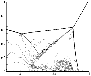
(a) WENO-AO(5,3)

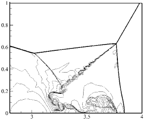
(b) WENO-AOA(5,3)

Figure 3: The enlarged view of the density contours of double Mach reflection problem at $t=0.28$ calculated by WENO-AO(5,3) and WENO-AOA(5,3) with $1601\times 401$ mesh points.

This problem is governed by the two-dimensional compressible Euler equations equipped with certain initial conditions and boundary conditions. It was originally proposed by Woodward and Colella [27] and was widely used to test the performance of numerical schemes for sophisticated structures and strong shocks. The specific settings can be found in Woodward and Colella [27] and many other papers, so we omit them for saving space in this note. We run this problem to $t=0.28$. Fig. 2 shows the entire view of the density contours calculated by WENO-AO(5,3) and WENO-AOA(5,3) with $1601\times 401$ mesh points. The overall profiles are the same, but the details of the reflecting zone are distinct as shown by Fig. 3. The difference is attributed to the intrinsical chaos characteristic of KelvinHelmholtz (KH) instabilities.

6 Conclusions

We proposed an alternative WENO-AO reconstruction which has a more concise form than the original WENO-AO reconstruction. In the benchmark tests, WENO-AOA performs similarly with WENO-AO. The main advantage of the WENO-AOA is the strict convexity that may make the reconstruction relatively reliable in general cases.

References

- [1] A. Harten, B. Engquist, S. Osher, S. R. Chakravarthy, Uniformly high order accurate essentially non-oscillatory schemes, III, Journal of Computational Physics 71 (2) (1987) 231–303. doi:10.1016/0021-9991(87)90031-3.
- [2] A. Harten, High resolution schemes for hyperbolic conservation laws, SIAM Review 49 (3) (1983) 357–393.
- [3] C.-W. Shu, S. Osher, Efficient implementation of essentially non-oscillatory shock-capturing schemes, Journal of Computational Physics 77 (1988) 439–471.
- [4] C.-W. Shu, S. Osher, Efficient implementation of essentially non-oscillatory shock-capturing schemes, ii, Journal of Computational Physics 83 (1989) 32–78.
- [5] X.-D. Liu, S. Osher, T. Chan, et al., Weighted essentially non-oscillatory schemes, Journal of computational physics 115 (1) (1994) 200–212.
- [6] G.-S. Jiang, C.-W. Shu, Efficient implementation of weighted ENO schemes, Journal of Computational Physics 126 (1) (1996) 202–228. doi:10.1006/jcph.1996.0130.
- [7] R. Borges, M. Carmona, B. Costa, W. S. Don, An improved weighted essentially non-oscillatory scheme for hyperbolic conservation laws, Journal of Computational Physics 227 (6) (2008) 3191–3211.
- [8] D. S. Balsara, C.-W. Shu, Monotonicity preserving weighted essentially non-oscillatory schemes with increasingly high order of accuracy, Journal of Computational Physics 160 (2) (2000) 405–452.
- [9] X. Deng, H. Zhang, Developing high-order weighted compact nonlinear schemes, Journal of Computational Physics 165 (1) (2000) 22–44.
- [10] F. Bianco, G. Puppo, G. Russo, High-order central schemes for hyperbolic systems of conservation laws, SIAM Journal on Scientific Computing 21 (1) (1999) 294–322.
- [11] D. Levy, G. Puppo, G. Russo, Central WENO schemes for hyperbolic systems of conservation laws, ESAIM: Mathematical Modelling and Numerical Analysis 33 (3) (1999) 547–571.
- [12] D. Levy, G. Puppo, G. Russo, Compact central WENO schemes for multidimensional conservation laws, SIAM Journal on Scientific Computing 22 (2) (2000) 656–672.
- [13] J. Qiu, C.-W. Shu, Hermite WENO schemes and their application as limiters for Runge–Kutta discontinuous Galerkin method: One-dimensional case, Journal of Computational Physics 193 (1) (2004) 115–135.
- [14] J. Qiu, C.-W. Shu, Hermite WENO schemes and their application as limiters for Runge–Kutta discontinuous Galerkin method II: Two-dimensional case, Computers & Fluids 34 (6) (2005) 642–663.
- [15] V. A. Titarev, E. F. Toro, ADER: Arbitrary high order Godunov approach, Journal of Scientific Computing 17 (1-4) (2002) 609–618.
- [16] V. A. Titarev, E. F. Toro, Finite-volume weno schemes for three-dimensional conservation laws, Journal of Computational Physics 201 (1) (2004) 238–260.
- [17] D. S. Balsara, C. Meyer, M. Dumbser, H. Du, Z. Xu, Efficient implementation of ADER schemes for Euler and magnetohydrodynamical flows on structured meshes–speed comparisons with Runge–Kutta methods, Journal of Computational Physics 235 (2013) 934–969. doi:10.1016/j.jcp.2012.04.051.
- [18] M. Dumbser, D. S. Balsara, E. F. Toro, C.-D. Munz, A unified framework for the construction of one-step finite volume and discontinuous Galerkin schemes on unstructured meshes, Journal of Computational Physics 227 (18) (2008) 8209–8253. doi:10.1016/j.jcp.2008.05.025.
- [19] M. Dumbser, O. Zanotti, Very high order schemes on unstructured meshes for the resistive relativistic MHD equations, Journal of Computational Physics 228 (18) (2009) 6991–7006.
- [20] M. Dumbser, Arbitrary high order schemes on unstructured meshes for the compressible Navier–Stokes equations, Computers & Fluids 39 (1) (2010) 60–76.
- [21] J. Zhu, J. Qiu, A new fifth order finite difference WENO scheme for solving hyperbolic conservation laws, Journal of Computational Physics 318 (2016) 110–121.
- [22] D. S. Balsara, S. Garain, C.-W. Shu, An efficient class of WENO schemes with adaptive order, Journal of Computational Physics 326 (2016) 780–804.
- [23] D. S. Balsara, S. Garain, V. Florinski, W. Boscheri, An efficient class of weno schemes with adaptive order for unstructured meshes, Journal of Computational Physics 404 (2020) 109062.
- [24] J. Zhu, C.-W. Shu, A new type of multi-resolution WENO schemes with increasingly higher order of accuracy, Journal of Computational Physics 375 (2018) 659–683.
- [25] J. Zhu, C.-W. Shu, A new type of multi-resolution WENO schemes with increasingly higher order of accuracy on triangular meshes, Journal of Computational Physics 392 (2019) 19–33.
- [26] J. Zhu, C.-W. Shu, A new type of third-order finite volume multi-resolution WENO schemes on tetrahedral meshes, Journal of Computational Physics 406 (2020) 109212.
- [27] P. Woodward, P. Colella, The numerical simulation of two-dimensional fluid flow with strong shocks, Journal of computational physics 54 (1) (1984) 115–173.