Construction of explicit symplectic integrators in general relativity. III. Reissner-Nordström-(anti)-de Sitter black holes

Abstract

We give a possible splitting method to a Hamiltonian for the description of charged particles moving around the Reissner-Nordström-(anti)-de Sitter black hole with an external magnetic field. This Hamiltonian can be separated into six analytical solvable pieces, whose solutions are explicit functions of proper time. In this case, second- and fourth-order explicit symplectic integrators are easily available. They exhibit excellent long-term behavior in maintaining the boundness of Hamiltonian errors regardless of ordered or chaotic orbits if appropriate step-sizes are chosen. Under some circumstances, an increase of positive cosmological constant gives rise to strengthening the extent of chaos from the global phase space; namely, chaos of charged particles occurs easily for the accelerated expansion of the universe. However, an increase of the magnitude of negative cosmological constant does not. The different contributions on chaos are because the cosmological constant acts as a repulsive force in the Reissner-Nordström-de Sitter black hole, but an attractive force in the Reissner-Nordström-anti-de Sitter black hole.

Unified Astronomy Thesaurus concepts: Black hole physics (159); Computational methods (1965); Computational astronomy (293); Celestial mechanics (211)

1 Introduction

Many exact solutions on black holes can be derived from Einstein’s general relativistic field equations. The first statical spherically symmetric solution is the Schwarzschild metric (Schwarzschild 1916). When the mass source in the origin has an electric charge, the Schwarzschild metric is the famous Reissner-Nordström (RN) solution (Reissner 1916; Nordström 1918). When a positive constant $\Lambda$ for describing the static cosmological model introduced by Einstein is included in the Schwarzschild metric, the Schwarzschild-de Sitter metric is provided. With the inclusion of cosmological constant $\Lambda$, the Reissner-Nordström-(anti)-de Sitter [RN-(A)dS] solution (Reissner 1916; Kottler 1918; Nordström 1918) is also obtained.

A small positive cosmological constant acts as a gravitationally repulsive energy component, and models dark energy for dominating the energy budget of the universe leads to an accelerated expansion of the universe (Ashtekar 2017). This result is strongly supported by observational evidences (Riess et al. 1998; Perlmutter et al. 1999; Ade et al. 2016). In fact, the cosmological constant describes a weak field gravity for the dynamics of galaxies, galaxy groups and clusters, and is supported by the parameters of galactic halos and of a sample of galaxy groups (Gurzadyan 2019; Gurzadyan $\&$ Stepanian 2019). Surprisingly, the theory of gravitational waves from isolated systems links up with the presence of a positive cosmological constant (Ashtekar et al. 2016; Ashtekar 2017). Although the known observational results do not support the existence of a negative cosmological constant, the negative cosmological constant becomes useful in the study of the black hole thermodynamics under the existence of quantum fields in gravitational fields. Appropriate boundary conditions should be imposed in black holes so that the black holes remain thermally stable. The AdS boundary, as a reflecting wall, can cause asymptotically AdS black holes to remain thermally stable. The phase transition between Schwarzschild AdS black holes and thermal AdS space was discovered by Hawking $\&$ Page (1983). Finite temperature configurations in the decoupled field theory are associated to black hole configurations in AdS spacetimes. The black holes yield the Hawking radiation in the AdS spacetime (Maldacena 1998). On the other hand, the cosmological constant affects some properties of accretion discs orbiting black holes in quasars and active galactic nuclei (Stuchlík 2005). These accretion discs are developed through the accretion process of dust and gases around compact objects. The mass of the accreting body increases during the accretion process, but it could also decrease (Jamil et al. 2008; Jamil 2009). Karkowski $\&$ Malec (2013) found that the damping effect on the mass accretion rate is weaker for positive values of the cosmological constant than for negative values of the cosmological constant, and it is related to the ratio of the dark energy density to the fluid density. The authors mainly focused on the question of how the cosmological constant exerts influences on the possible accretion rate. Ficek (2015) considered relativistic Bondi-type accretion in the RN-(A)dS spacetime.

The Schwarzschild, RN and RN-(A)dS spacetimes are highly nonlinear, but they are integrable and non-chaotic. Magnetic fields can destroy the integrability of these spacetimes. In fact, a strong magnetic field with hundred Gauss is indeed present in the vicinity of the supermassive black hole at the Galactic center (Eatough et al. 2013). The presence of an external magnetic field was shown through high-frequency quasiperiodic oscillations and relativistic jets observed in microquasars (Stuchlík et al. 2013; Kološ et al. 2017). It can influence oscillations in the accretion disk and the creation of jets. The accretion of charged particles from the accretion disk goes towards the black hole due to a radiation-reaction force. The external magnetic field that is usually considered is so weak that it does not perturb a spacetime metric; namely, the external magnetic field does not appear in the spacetime metric and is not a solution of the field equations of general relativity. However, such weak magnetic field will essentially affect motions of electrons or protons when the ratios of charges of electrons or protons to masses of electrons or protons are large (Tursunov et al. 2018). Of course, some magnetic fields can perturb spacetime metrics, such as the magnetized Ernst-Schwarzschild spacetime geometry (Ernst 1976). The chaotic motions of charged particles around the Schwarzschild and Kerr black holes were confirmed in a series of papers (Nakamura $\&$ Ishizuka 1993; Takahashi $\&$ Koyama 2009; Kopáček et al. 2010; Kopáček $\&$ Karas 2014; Stuchlík $\&$ Kološ 2016; Kopáček $\&$ Karas 2018; Pánis et al. 2019; Stuchlík et al. 2020; Yi $\&$ Wu 2020). In particular, the chaotic dynamics of neutral particles in the magnetized Ernst-Schwarzschild spacetim is possible due to the magnetic field acting as a gravitational effect although no electromagnetic forces exist (Karas $\&$ Vokroulflický 1992; Li $\&$ Wu 2019). Besides external magnetic fields, spin of particles is an important source for inducing chaos. Chaos can occur when a spinning test particle moves in the spacetime background of a Kerr black hole (Lukes-Gerakopoulos et al. 2016). Resonances and chaos for spinning test particles in the Schwarzschild and Kerr backgrounds were shown by Brink et al. (2015a, b) and Zelenka et al. (2020). Some spacetime backgrounds, e.g., the Manko, Sanabria-Gómez, Manko (MSM) metric can be chaotic (Dubeibe et al. 2007; Han 2008; Seyrich $\&$ Lukes-Gerakopoulos 2012). The word “chaos” is a nonlinear behavior of a dynamical system and describes the system with exponentially sensitive dependence on initial conditions. The chaotic or regular feature of orbital motions can be reflected on the gravitational waves (Zelenka et al. 2019).

Detecting the chaotical behavior requires that a numerical integration scheme have good stability and precision, i.e., provide reliable results to the trajectories. The Schwarzschild, RN and RN-(A)dS spacetimes are integrable, but their solutions are unknown. Thus, numerical schemes are still necessary to solve these systems. It is well known that symplectic integrators are the most appropriate solvers for long-term evolution of Hamiltonian systems. Clearly, Hamiltonians of the Schwarzschild, RN and RN-(A)dS spacetimes are not separations of variables. Perhaps each of the Hamiltonians may be split into two integrable parts, but no explicit functions of proper time can be given to analytical solutions of the two parts in the general case. Explicit symplectic integrators (Swope et al. 1982; Wisdom 1982; Ruth 1983; Forest $\&$ Ruth 1990; Wisdom $\&$ Holman 1991) that have been developed in the solar system and share good long-term numerical performance in the preservation of geometric structures and constants of motion become useless in this case. However, completely implicit or explicit and implicit combined symplectic integrators should be available without doubt (Brown 2006; Preto $\&$ Saha 2009; Kopáček et al. 2010; Lubich et al. 2010; Zhong et al. 2010; Mei et al. 2013a, 2013b; Tsang et al. 2015). In most cases, explicit algorithms have advantage over same order implicit schemes at the expense of computational time. Considering this point, we proposed second- and fourth-order explicit symplectic integration algorithms for the Schwarzschild spacetime by separating the Hamiltonian of this spacetime into four parts with analytical solutions as explicit functions of proper time in Paper I (Wang et al. 2021a). When five parts similar to the four separable pieces in the Hamiltonian of the Schwarzschild metric are given to a splitting form of the Hamiltonian of the RN black hole with an external magnetic field, explicit symplectic integrators were also set up in Paper II (Wang et al. 2021b). In other words, a fact concluded from Papers I and II is that the construction of explicit symplectic integrations is possible for a curved spacetime when a Hamiltonian of the spacetime is separated into more parts with analytical solutions as explicit functions of proper time. How to split the Hamiltonian depends on what this spacetime is.

Following Papers I and II, we want to know in this paper how explicit symplectic integrators are designed for the RN-(A)dS spacetime with an external magnetic field. We are particularly interested in investigating how the cosmological constant effects the regular and chaotic dynamical behavior of charged particles moving around the black hole. For the sake of these purposes, we introduce the relativistic gravitational field in Sect. 2. In Sect. 3, we give new explicit symplectic integrators and check their numerical performance. Then, a new explicit symplectic method with an appropriate step size is applied to survey the effect of the cosmological constant on the dynamics of orbits of charged particles. Finally, the main results are concluded in Sect. 4.

2 RN black hole with cosmological constant and external magnetic field

In dimensionless spherical-like coordinates $(t,r,\theta,\phi)$, the RN black hole with electric charge $Q$ and cosmological constant $\Lambda$ describing the expansion of the universe is given in the following spacetime (Ahmed et al. 2016)

$$-\tau^{2} = ds^{2}=g_{\alpha\beta}dx^{\alpha}dx^{\beta}$$ (1)

$$= -(1-\frac{2}{r}+\frac{Q^{2}}{r^{2}}-\frac{\Lambda}{3}r^{2})dt^{2}$$

$$+(1-\frac{2}{r}+\frac{Q^{2}}{r^{2}}-\frac{\Lambda}{3}r^{2})^{-1}dr^{2}$$

$$+r^{2}d\theta^{2}+r^{2}\sin^{2}\theta d\phi^{2}.$$

Here, geometrized units $c=G=M=1$ are given to the speed of light $c$, the constant of gravity $G$, and the mass of black hole $M$. Dimensionless operations act on proper time $\tau$, coordinate time $t$, separation $r$, charge $Q$, and cosmological constant $\Lambda$. Namely, $\tau\rightarrow M\tau$, $t\rightarrow Mt$, $r\rightarrow Mr$, $Q\rightarrow MQ$ and $\Lambda\rightarrow\Lambda/M^{2}$. The four-velocity $\mathbf{U}=U^{\mu}=\dot{x}^{\mu}$ is also dimensionless and satisfies the constraint

$$\mathbf{U}\bullet\mathbf{U}=U^{\alpha}U_{\alpha}=g_{\mu\nu}\dot{x}^{\mu}\dot{x}^{\nu}=-1.$$ (2)

Unlike the Euclid inner product, the Riemann inner product $\bullet$ in Eq. (2) can be negative.

$\Lambda=0$ indicates that Equation (1) is an asymptotically flat metric. A non-vanishing cosmological constant $\Lambda$ represents a weak field gravity proper for the dynamics of galaxies, galaxy groups and clusters. $\Lambda>0$ and $\Lambda<0$ correspond to asymptotically de Sitter (dS) and anti-de Sitter (AdS) spacetimes, respectively. Without loss of generality, we consider a relation between realistic and dimensionless values of positive cosmological constant. The realistic value of cosmological constant obtained by Planck data is $\Lambda_{PL}=1.11\times 10^{-52}m^{-2}=1.11\times 10^{-46}km^{-2}$ (Ade et al. 2016). Various realistic values of cosmological constant for dark matter considering the data on galaxy systems from galaxy pairs to galaxy clusters were given in the range $\Lambda=10^{-52}m^{-2}\sim 10^{-50}m^{-2}$ (Gurzadyan $\&$ Stepanian 2019). Suppose that the value $\Lambda_{0}=10^{-46}km^{-2}$ considered in a paper of Xu $\&$ Wang (2017) is regarded as a realistic value of cosmological constant, a dimensionless value of cosmological constant can be estimated in terms of $\Lambda=\Lambda_{0}M^{2}G^{2}/c^{4}$. Obviously, it depends on the mass of a black hole. For the supermassive black hole candidate in the center of the giant elliptical galaxy M87 having mass $M=(6.5\pm 0.7)\times 10^{9}M_{\odot}$ with $M_{\odot}$ being the Sun’s mass (EHT Collaboration et al. 2019a, b, c), we obtain dimensionless cosmological constant $\Lambda=\Lambda_{0}M^{2}G^{2}/c^{4}=10^{-46}km^{-2}\times[(6.5\pm 0.7)\times 10^{9}M_{\odot}G/c^{2}]^{2}=10^{-46}km^{-2}\times(6.5\pm 0.7)^{2}\times 10^{18}\times 1.475^{2}km^{2}=7.3\times 10^{-27}\sim 1.1\times 10^{-26}$. Such a small dimensionless value does not change the spacetime geometry of black hole if the separation $r$ is not large enough. The effect of cosmological constant on the spacetime should also be negligible for the $150M_{\odot}$ binary black hole merger GW190521 (Abbott et al. 2020a, 2020b). The dimensionless value of cosmological constant increases with an increase of the black hole’s mass. If the black hole’s mass is $M=(1/1.475)\times 10^{20}M_{\odot}$, we have dimensionless cosmological constant $\Lambda=10^{-6}$. For $M=(1/1.475)\times 10^{21}M_{\odot}$, $\Lambda=10^{-4}$. Given $M=2.14391705774127\times 10^{22}M_{\odot}$, $\Lambda=0.1$. When $M=(1/1.475)\times 10^{23}M_{\odot}$, $\Lambda=1$. These larger dimensionless values should exert explicit influences on the spacetime geometries. The larger dimensionless values of cosmological constant (e.g. $\Lambda=-0.075,-0.1,0.1$) in the references (Ahmed et al. 2016; Shahzad $\&$ Jawad 2019; Shafiq et al. 2020) may be taken for the existence of extremely supermassive black holes. In what follows, various values of cosmological constant are dimensionless. Equation (1) is called the RN-(A)dS spacetime. It has at most three event horizons (Ahmed et al. 2016; Shahzad $\&$ Jawad 2019).

Seen from the expression $g_{00}=-1-2\varphi$ ($\varphi$ is the gravitational potential) in Eq. (1), the potential $-1/r$ plays a role in an attractive force proportional to $-1/r^{2}$. Similarly, the cosmological constant makes the potential $-\Lambda r^{2}/6$ yield an attractive force proportional to $\Lambda r/3$ for $\Lambda<0$, but a repulsive force for $\Lambda>0$. The force is independent of the black hole’s mass. However, the black hole’s charge leads to the potential $Q^{2}/(2r^{2})$ giving a repulsive force proportional to $Q^{2}/r^{3}$. As the distance increases, the attraction from the heavy body and the repulsive force from the charge decrease; the latter is smaller than the former. However, the attraction or repulsiveness from the cosmological constant grows. It eventually dominates the other two forces when the distance is large enough.

The metric corresponds to a Lagrangian system

$$\mathcal{L}=\frac{1}{2}(\frac{ds}{d\tau})^{2}=\frac{1}{2}g_{\mu\nu}\dot{x}^{\mu}\dot{x}^{\nu}.$$ (3)

It defines a covariant generalized momentum

$$p_{\mu}=\frac{\partial\mathcal{L}}{\partial\dot{x}^{\mu}}=g_{\mu\nu}\dot{x}^{\nu}.$$ (4)

Since the Lagrangian does not explicitly depend on $t$ and $\phi$, the Euler-Lagrangian equations show that two constant momentum components with respect to proper time $\tau$ are

$$p_{t} = -(1-\frac{2}{r}+\frac{Q^{2}}{r^{2}}-\frac{\Lambda}{3}r^{2})\dot{t}=-\mathbb{E},$$ (5)

$$p_{\phi} = r^{2}\sin^{2}\theta\dot{\phi}=\mathbb{L}.$$ (6)

$\mathbb{E}$ is the energy of a test particle moving in the gravitational field, and $\mathbb{L}$ denotes the angular momentum of the particle.

Transform the Lagrangian into a Hamiltonian

$$H = \mathbf{U}\bullet\mathbf{p}-\mathcal{L}=\frac{1}{2}g^{\mu\nu}p_{\mu}p_{\nu}$$ (7)

$$= -\frac{1}{2}(1-\frac{2}{r}+\frac{Q^{2}}{r^{2}}-\frac{\Lambda}{3}r^{2})^{-1}\mathbb{E}^{2}$$

$$+\frac{1}{2}(1-\frac{2}{r}+\frac{Q^{2}}{r^{2}}-\frac{\Lambda}{3}r^{2})p^{2}_{r}+\frac{1}{2}\frac{p^{2}_{\theta}}{r^{2}}$$

$$+\frac{1}{2}\frac{\mathbb{L}^{2}}{r^{2}\sin^{2}\theta}.$$

Due to Eq. (2), this Hamiltonian is always identical to a given constant

$$H=-\frac{1}{2}.$$ (8)

In fact, a second integral (Carter 1968) excluding $E$ and $\mathbb{L}$ can be found by the variables separated in the Hamilton-Jacobi equation. Thus, this system is integrable.

Let the black hole suffer from the interaction of an external magnetic field. The electromagnetic field is described by a four-vector potential with two nonzero covariant components (Felice $\&$ Sorge 2003; Wang $\&$ Zhang 2020)

$$A_{t} = -\frac{Q}{r},$$ (9)

$$A_{\phi} = \frac{B}{2}g_{\phi\phi}=\frac{B}{2}r^{2}\sin^{2}\theta.$$ (10)

$A_{t}$ is the Coulomb part of the electromagnetic potential. It does not appear in the metric $g_{\alpha\beta}$, but it should be given because a charged particle and the black hole’s charge $Q$ yields a Coulomb force. This Coulomb force is compensated by $A_{t}$. $B$ denotes the strength of the magnetic field parallel to the $z$ axis. As claimed in the Introduction, $B$ is so weak that it does not affect the metric but affects the motion of charged particles. The motion of particles with charge $q$ around the magnetized black hole is determined by the Hamiltonian

$$K = \frac{1}{2}g^{\mu\nu}(p_{\mu}-qA_{\mu})(p_{\nu}-qA_{\nu})$$ (11)

$$= -\frac{1}{2}(1-\frac{2}{r}+\frac{Q^{2}}{r^{2}}-\frac{\Lambda}{3}r^{2})^{-1}(E-\frac{\tilde{Q}}{r})^{2}$$

$$+\frac{1}{2}(1-\frac{2}{r}+\frac{Q^{2}}{r^{2}}-\frac{\Lambda}{3}r^{2})p^{2}_{r}+\frac{1}{2}\frac{p^{2}_{\theta}}{r^{2}}$$

$$+\frac{L^{2}}{2r^{2}\sin^{2}\theta}+\frac{1}{8}\beta^{2}r^{2}\sin^{2}\theta-\frac{\beta L}{2},$$

where $Q^{*}=qQ$ and $\beta=qB$. Dimensionless operations (see also Yi $\&$ Wu 2020) are given as follows: $K\rightarrow Km^{2}_{p}$, $E\rightarrow Em_{p}$, $p_{r}\rightarrow p_{r}m_{p}$, $p_{\theta}\rightarrow p_{\theta}Mm_{p}$, $L\rightarrow LMm_{p}$, $B\rightarrow B/M$ and $q\rightarrow qm_{p}$, where $m_{p}$ is the particle’s mass. Unlike $\mathbb{E}$ and $\mathbb{L}$ in Eqs. (5) and (6), the energy $E$ and angular momentum $L$ are written as

$$E = (1-\frac{2}{r}+\frac{Q^{2}}{r^{2}}-\frac{\Lambda}{3}r^{2})\dot{t}+\frac{Q^{*}}{r},$$ (12)

$$L = r^{2}\sin^{2}\theta\dot{\phi}+\frac{1}{2}\beta r^{2}\sin^{2}\theta.$$ (13)

The magnetic field causes the radial potential $\beta^{2}r^{2}/8$ to yield an attractive force proportional to $-\beta^{2}r/4$. The attraction grows with the distance. However, the radial potential $L^{2}/(2r^{2})$ from the angular momentum gives a repulsive force proportional to $L^{2}/r^{3}$. In fact, this repulsive force is a centrifugal force of inertia. As Wang et al. (2021b) claimed, the Coulomb term gives the particle a repulsive force effect for $Q^{*}>0$, but a gravitational force effect for $Q^{*}<0$. It is more important than the repulsive force effect from the black hole’s charge. Although the potential from the black hole’s charge and the potential from the angular momentum yield the repulsive forces, the latter repulsive forces vary their directions when the charged particles’ motions are not restricted to the radial motions. Similarly, the attractive forces from the magnetic field unlike those from the negative cosmological constant (or those from the heavy body) have also different directions in the general case.

The Hamiltonian $K$ is still equal to the given constant

$$K=-\frac{1}{2}.$$ (14)

However, no second integral excluding the two integrals $E$ and $L$ exists in the case. Thus, this Hamiltonian is non-integrable. Its dynamics is complicated and mainly employs numerical techniques to be investigated.

3 Numerical investigations

First, new explicit symplectic integrators are specifically designed for the Hamiltonian system (11). Then, the performance of the new algorithms is evaluated. Finally, the dynamics of order and chaos of orbits in the Hamiltonian is surveyed, and the relation between the chaotic behavior and the cosmological constant is mainly discussed.

3.1 Construction of explicit symplectic integrators

In Papers I and II (Wang et al. 2021a, b), the explicit symplectic integrators were proposed for the Hamiltonian of Schwarzschild’s metric with four analytical integrable splitting parts, and the Hamiltonian of RN’s metric with five analytical integrable separable parts. These successful examples in general relativity tell us that the key of the construction of an explicit symplectic integrator lies in splitting the considered Hamiltonian in an appropriate way. Not only the splitting parts in this Hamiltonian should be analytically solvable, but also all analytical solutions in the separable parts should be explicit functions of proper time $\tau$. Noticing this idea, we begin our work.

Split the Hamiltonian (11) into six parts

$$K=K_{1}+K_{2}+K_{3}+K_{4}+K_{5}+K_{6}.$$ (15)

The sub-Hamiltonians are expressed as

$$K_{1} = -\frac{1}{2}(1-\frac{2}{r}+\frac{Q^{2}}{r^{2}}-\frac{\Lambda}{3}r^{2})^{-1}(E-\frac{Q^{*}}{r})^{2}$$ (16)

$$+\frac{L^{2}}{2r^{2}\sin^{2}\theta}+\frac{1}{8}\beta^{2}r^{2}\sin^{2}\theta-\frac{\beta L}{2},$$

$$K_{2} = \frac{1}{2}p^{2}_{r},$$ (17)

$$K_{3} = -\frac{1}{r}p^{2}_{r},$$ (18)

$$K_{4} = \frac{p^{2}_{\theta}}{2r^{2}},$$ (19)

$$K_{5} = \frac{1}{2}\frac{Q^{2}}{r^{2}}p^{2}_{r},$$ (20)

$$K_{6} = -\frac{\Lambda}{6}r^{2}p^{2}_{r}.$$ (21)

$K_{2}$, $K_{3}$, $K_{4}$ and $K_{5}$ are consistent with those in the decomposing method of the RN black hole in Paper II (Wang et al. 2021b).

$K_{1}$, $\cdots$, $K_{6}$ correspond to differential operators $\mathcal{A}$, $\mathcal{B}$, $\mathcal{C}$, $\mathcal{D}$, $\mathcal{E}$ and $\mathcal{F}$, respectively. These operators are written in the forms

$$\mathcal{A} = -\frac{\partial K_{1}}{\partial r}\frac{\partial}{\partial p_{r}}-\frac{\partial K_{1}}{\partial\theta}\frac{\partial}{\partial p_{\theta}}$$ (22)

$$= [-(E-\frac{Q^{*}}{r})^{2}(\frac{1}{r^{2}}-\frac{Q^{2}}{r^{3}}-\frac{\Lambda}{3}r)$$

$$\cdot(1-\frac{2}{r}+\frac{Q^{2}}{r^{2}}-\frac{\Lambda}{3}r^{2})^{-2}$$

$$+\frac{Q^{*}}{r^{2}}(E-\frac{Q^{*}}{r})(1-\frac{2}{r}+\frac{Q^{2}}{r^{2}}-\frac{\Lambda}{3}r^{2})^{-1}$$

$$+\frac{L^{2}}{r^{3}\sin^{2}\theta}-\frac{\beta^{2}}{4}r\sin^{2}\theta]\frac{\partial}{\partial p_{r}}$$

$$+(\frac{L^{2}\cos\theta}{r^{2}\sin^{3}\theta}-\frac{1}{8}\beta^{2}r^{2}\sin(2\theta))\frac{\partial}{\partial p_{\theta}}$$

$$= f_{1}(r,\theta)\frac{\partial}{\partial p_{r}}+f_{2}(r,\theta)\frac{\partial}{\partial p_{\theta}},$$

$$\mathcal{B} = p_{r}\frac{\partial}{\partial r},$$ (23)

$$\mathcal{C} = -\frac{2}{r}p_{r}\frac{\partial}{\partial r}-\frac{p^{2}_{r}}{r^{2}}\frac{\partial}{\partial p_{r}},$$ (24)

$$\mathcal{D} = \frac{p_{\theta}}{r^{2}}\frac{\partial}{\partial\theta}+\frac{p^{2}_{\theta}}{r^{3}}\frac{\partial}{\partial p_{r}},$$ (25)

$$\mathcal{E} = \frac{Q^{2}}{r^{2}}p_{r}\frac{\partial}{\partial r}+Q^{2}\frac{p^{2}_{r}}{r^{3}}\frac{\partial}{\partial p_{r}},$$ (26)

$$\mathcal{F} = -\frac{\Lambda}{3}r^{2}p_{r}\frac{\partial}{\partial r}+\frac{\Lambda}{3}rp^{2}_{r}\frac{\partial}{\partial p_{r}}.$$ (27)

Using them to act on the solutions $\textbf{z}(0)=(r_{0},\theta_{0},p_{r0},p_{\theta 0})$ at the beginning of proper time step $h$, we can obtain their corresponding analytical solutions $\textbf{z}=(r,\theta,p_{r},p_{\theta})$ over a step size $h$. All the analytical solutions are indeed explicit functions of the proper time step $h$. For example, the analytical solutions z for the sub-Hamiltonian $K_{1}$ are expressed in an exponential operator $e^{h\mathcal{A}}$ as $\textbf{z}=(p_{r},p_{\theta})=e^{h\mathcal{A}}\textbf{z}(0)$. That is, $p_{r}=p_{r0}+hf_{1}(r_{0},\theta_{0})$ and $p_{\theta}=p_{\theta 0}+hf_{2}(r_{0},\theta_{0})$. These exponential operators symmetrically compose a second-order explicit symplectic integrator

$$S^{K}_{2}(h) = e^{\frac{h}{2}\mathcal{F}}\circ e^{\frac{h}{2}\mathcal{E}}\circ e^{\frac{h}{2}\mathcal{D}}\circ e^{\frac{h}{2}\mathcal{C}}\circ e^{\frac{h}{2}\mathcal{B}}\circ e^{h\mathcal{A}}$$ (28)

$$\circ e^{\frac{h}{2}\mathcal{B}}\circ e^{\frac{h}{2}\mathcal{C}}\circ e^{\frac{h}{2}\mathcal{D}}\circ e^{\frac{h}{2}\mathcal{E}}\circ e^{\frac{h}{2}\mathcal{F}}.$$

This explicit symplectic method is specifically designed for the Hamiltonian (11). It is easily used to yield a fourth-order symplectic scheme of Yoshida (1990)

$$S^{K}_{4}(h)=S^{K}_{2}(\gamma h)\circ S^{K}_{2}(\delta h)\circ S^{K}_{2}(\gamma h),$$ (29)

where $\delta=1-2\gamma$ and $\gamma=1/(2-\sqrt[3]{2})$.

Here are three points illustrated. (i) the Hamiltonian (11) becomes the RN Hamiltonian (7) for the case of $\beta=0$. It is natural that the newly established algorithms are appropriate for the RN problem. (ii) The splitting technique to the Hamiltonian (11) may not be unique. Perhaps there may be other splitting methods that satisfy the requirement for the construction of such similar explicit symplectic integration algorithms. (iii) The present operator splitting method can be applied to an extended version of the Hamiltonian (11) as follows:

$$\Gamma = f_{1}(r,\theta)+g^{rr}p^{2}_{r}+g^{\theta\theta}p^{2}_{\theta\theta},$$ (30)

$$g^{rr} = (a_{0}+a_{1}r+\cdots+a_{n}r^{n}+\frac{b_{1}}{r}+\frac{b_{2}}{r^{2}}$$

$$+\cdots+\frac{b_{m}}{r^{m}})f_{2}(\theta),$$

$$g^{\theta\theta} = f_{3}(r),$$

where $f_{1}$, $f_{2}$ and $f_{3}$ are arbitrary continuous differentiable functions when $r$ is restricted to $r>2$, and $a_{0}$, $\cdots$, $a_{n}$, $b_{1}$, $\cdots$, $b_{m}$ are constant parameters. For the Kerr metric, the operator splitting method is not available because the denominators of $g^{rr}$ and $g^{\theta\theta}$ are $r^{2}+a^{2}\cos^{2}\theta$. Similarly, the method becomes useless for the magnetized Ernst-Schwarzschild spacetime (Ernst 1976).

3.2 Numerical evaluations

Now, let us apply the second-order explicit symplectic method S2 or the fourth-order method S4 to work out the magnetized RN-dS spacetime (11). We take the parameters $E=0.975$, $L=4.2$, $\beta=8\times 10^{-3}$, $Q=0.3$, $Q^{*}=1\times 10^{-6}$, and $\Lambda=2\times 10^{-6}$. A test orbit has initial conditions $r=25$, $p_{r}=0$ and $\theta=\pi/2$. The starting value of $p_{\theta}>0$ is determined by Eq. (14). Proper time step $h=1$ is adopted. It can be seen clearly from Fig. 1 (a) that algorithm S2 performs bounded Hamiltonian errors $\Delta K=-1/2-K$ with an order of $\mathcal{O}(10^{-6})$ in a long numerical integration of $10^{9}$ steps. The errors of S4 are smaller in 3 orders than those of S2, but have a slightly secular drift due to roundoff errors. Fortunately, this secular error growth is absent when a larger proper time step $h=4$ is used in the fourth-order method S4*. The fourth-order algorithm with the larger time step $h=4$ is the same as the second-order method with the smaller time step $h=1$ in the order of Hamiltonian errors. The former efficiency is 4/3 times faster than the latter one.

In fact, the test orbit is a regular orbit colored red in Fig. 1 (b). This regular orbit seems to consist of 7 loops on Poincaré section at the plane $\theta=\pi/2$ and $p_{\theta}>0$ (note that the 7 loops are unclearly visible). The order of Hamiltonian errors for each algorithm is not altered when the red regular orbit is replaced with the green regular orbit, blue regular orbit, or black weak chaotic orbit in Fig. 1 (b). In other words, the algorithms’ accuracies are independent of dynamical behavior of orbits. In what follows, we use the second-order method S2 with the smaller time step $h=1$ to trace the dynamics of order and chaos of orbits.

3.3 Dynamical transition with a variation of the cosmological constant

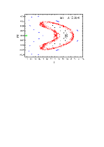
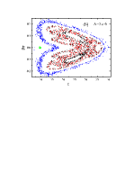
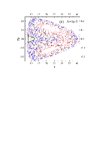
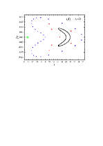
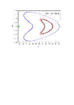
Figure 2: Same as Fig. 1 (b) but for different values of cosmological constant $\Lambda$.

To show cosmological constant $\Lambda$ how to affect the orbital dynamics of the system (11), we consider $\Lambda$ to increase. The red orbit is regular for $\Lambda=2\times 10^{-6}$ in Fig. 1 (b), but chaotic for $\Lambda=2.1\times 10^{-6}$ in Fig. 2 (a). The extent of chaos in Figs. 2 (b) and (c) is further strengthened with an increase of positive cosmological constant $\Lambda$. In fact, strong chaos occurs for $\Lambda=1\times 10^{-5}$. However, no chaos exists for $\Lambda=0$ in Fig. 2 (d). In particular, the red orbit is clearly composed of 7 small islands and is approximately a periodic orbit in this case. These results seem to show that chaos gets stronger as a positive cosmological constant increases. For negative cosmological constants, such as $\Lambda=-5\times 10^{-6}$ and $\Lambda=-1\times 10^{-5}$ in Figs. 2 (e) and (f), chaos is absent, either.

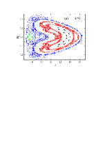
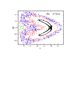
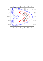
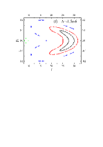
Figure 3: Same as Fig. 2 but magnetic parameter $\beta=9\times 10^{-3}$ is fixed.

The magnetic parameter $\beta=8\times 10^{-3}$ is taken in Figs. 1 and 2. What about the dynamics of the system (11) when $\beta$ gets slightly larger? For $\beta=9\times 10^{-3}$ with $\Lambda=0$ in Fig. 3 (a), two strong chaotic orbits exist, but do not for $\beta=8\times 10^{-3}$ with $\Lambda=0$ in Fig. 2 (d). As the positive cosmological constant further increases, chaos is easier to occur. For $\Lambda=2\times 10^{-6}$ in Fig. 3 (b), three chaotic orbits are present. For $\Lambda=1\times 10^{-5}$ in Fig. 3 (c), the four orbits are chaotic. However, an increase of the magnitude of negative cosmological constant weakens the extent of chaos. For example, two weak chaotic orbits exist for $\Lambda=-1.2\times 10^{-6}$ in Fig. 3 (e). When $\Lambda=-1.5\times 10^{-6}$ in Fig. 3 (f), no orbits can be chaotic.

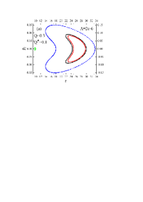
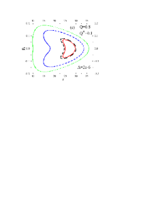
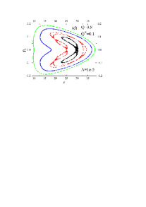
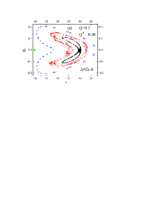
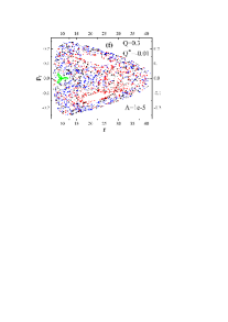
Figure 4: Same as Fig. 2 but different combinations of parameters $Q$, $Q^{*}$ and $\Lambda$ are given.

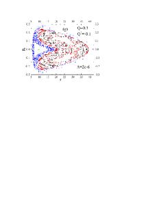
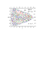
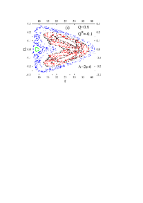
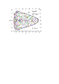
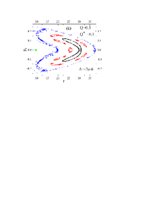
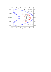
Figure 5: Fig. 4 continued.

The aforementioned demonstrations are based on the choice of a small value of the Coulomb parameter $Q^{*}$. Now, let us focus on the orbital dynamical transition when larger values of $Q^{*}$ are considered. Comparisons between Figs. 4 (a) and (b), Figs. 4 (c) and (d), Figs. 4 (e) and (f), Figs. 5 (g) and (h), and Figs. 5 (i) and (j) still consistently support the result that chaos becomes easier with an increase of positive cosmological constant $\Lambda$. In particular, this result is irrespective of whether $Q$ and $Q^{*}$ are larger or smaller, and $Q^{*}$ is positive or negative. However, an increase of the magnitude of negative cosmological constant leads to suppressing the occurrence of chaos or weakening the extent of chaos, as shown by the comparison between Figs. 5 (k) and (l). The chaos weakened is qualitatively observed from the Poincaré section. The blue orbit is chaotic for $\Lambda=-2\times 10^{-6}$ in panel (k), but it is not for $\Lambda=-1\times 10^{-5}$ in panel (l). In addition, other results are visible in Figs. 4 and 5. Figs. 1 (b), 2 (c), and 4 (a) and (b) describe that chaos is gradually weakened as a positive Coulomb parameter $Q^{*}$ increases. And chaos is much easily induced when the magnitude of negative Coulomb parameter increases. See Figs. 4 (e) and (f), and 5 (g) and (h) for more details. These results are consistent with those of Paper II (Wang et al. 2021b). As another one of the main results in Paper II, an increase of $Q$ does not exert a typical influence on the occurrence of chaos but twists the shape of orbits (such as the green orbit). This result is also confirmed by the comparisons among Figs. 4 (a)-(d), and 5 (g)-(j).

It can be concluded from Figs. 1 (b), 2, 3, 4 and 5 that an increase of positive cosmological constant (or an increase of the magnitude of negative Coulomb parameter $Q^{*}$) leads to strengthening the extent of chaos from the global phase space. However, an increase of the magnitude of negative cosmological constant (or an increase of positive Coulomb parameter $Q^{*}$) does not. These results can be explained similarly with the aid of slightly modified Equation (36) in Paper II:

$$K_{1} \approx -\frac{1}{2}(\beta L+E^{2})-\frac{\Lambda}{6}Q^{*2}-\frac{1}{6}\Lambda E^{2}r^{2}$$ (31)

$$+\frac{1}{3}\Lambda EQ^{*}r-\frac{E^{2}}{r}+\frac{\beta^{2}}{8}r^{2}\sin^{2}\theta$$

$$+\frac{EQ^{*}}{r}+\frac{Q^{2}E^{2}}{2r^{2}}+\frac{L^{2}}{2r^{2}\sin^{2}\theta}$$

$$+\frac{Q^{*}}{2r^{2}}(4E-Q^{*})+\cdots.$$

The third and fourth terms in the potential (31) correspond to the forces associated with the cosmological constant. The third term denominates the fourth term. It acts as a repulsive force for the RN-dS black hole. The repulsive force reduces the attractive force given by the potential $-E^{2}/r$ of the black hole. However, the third term yields an attractive force for the RN-AdS black hole. The attractive force enhances the attractive force from the black hole. On the other hand, the potential $EQ^{*}/r$ corresponds to the Coulomb force from the Coulomb part of the magnetic field potential. For $Q^{*}>0$, the Coulomb force is a repulsive force, which weakens the Lorentz force as an attractive force determined by the potential $\beta^{2}r^{2}\sin^{2}\theta/8$ of the magnetic field. However, the Coulomb force is an attractive force for $Q^{*}<0$. This leads to enhancing the attractive force from the magnetic field. Clearly, the Coulomb force from the Coulomb part of the magnetic field potential is larger than the repulsive force governed by the potential $Q^{2}E^{2}/(2r^{2})$ from the black hole’s charge. Only when the gravitational attractions of charged particles from the black hole and the magnetic field are approximately balanced, may chaos occur. Therefore, chaos is easily caused in some circumstances when any one of the positive cosmological constant, the magnitude of negative Coulomb parameter, and the magnetic field parameter increases.

4 Conclusion

The Hamiltonian for the description of charged particles moving around the RN-(A)dS black hole with an external magnetic field can be split into six parts, which have analytical solutions as explicit functions of proper time. In this case, second- and fourth-order explicit symplectic integration methods are easily designed for this Hamiltonian system.

It is shown via numerical simulations that the newly proposed algorithms with appropriate choices of step-sizes perform good long-term performance in maintaining the boundness of Hamiltonian errors. The result should always be the same, regardless of whether a test orbit is regular or chaotic.

The cosmological constant in the RN-dS black hole acts as a repulsive force, which weakens the gravitational force of charged particle from the black hole. As a result, the extent of chaos is strengthened from the global phase space when a positive cosmological constant increases. In other words, the accelerated expansion of the universe can easily induce chaos of charged particles in some cases. However, chaos is weakened when the magnitude of negative cosmological constant increases. This is because the cosmological constant in the RN-AdS black hole acts as an attractive force, which causes the gravitational effect from the black hole to dominate the attractive force from the magnetic field. For the presence of chaos in the present metric background, the effect of the cosmological constant on the accretion rate or the gravitational waves will be worth considering.

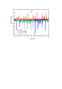
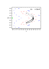
Figure 1: (a) Hamiltonian errors $\Delta K=-1/2-K$ for the new explicit symplectic algorithms solving the magnetized RN-dS spacetime (11). The parameters $E=0.975$, $L=4.2$, $\Lambda=2\times 10^{-6}$, $\beta=8\times 10^{-3}$, $Q=0.3$ and $Q^{*}=1\times 10^{-6}$ are used, and the initial conditions of a test orbit are $r=25$, $p_{r}=0$ and $\theta=\pi/2$ with the starting value of $p_{\theta}>0$ determined by Eq. (14) are chosen. The second-order method S2 and the fourth-order method S4 take proper time step $h=1$. The realistic errors for S4 are 1000 times smaller than the plotted errors. The errors for S2 are stabilized in an order of $\mathcal{O}(10^{-6})$, whereas do not remain bounded for S4 due to roundoff errors. Fortunately, such a secular drift in Hamiltonian errors lose when a larger time step $h=4$ is used in method S4*. (b) Poincaré sections on the plane $\theta=\pi/2$ and $p_{\theta}>0$, given by algorithm S2 with proper time step $h=1$. The test orbit in panel (a) is a regular orbit colored red in panel (b). The other three orbits are regular tori colored green with initial separation $r=10$ and blue with initial separation $r=18$, and a weak chaotic orbit colored black with initial separation $r=30$.

References

- Abbott et al. (2020a) Abbott, R., Abbott, T. D., Abraham, S., et al. 2020a, ApJL, 900, L13
- Abbott et al. (2020b) Abbott, R., Abbott, T. D., Abraham, S., et al. 2020b, Phys. Rev. Lett., 125, 101102
- Ade et al. (2016) Ade, P. A. R., Aghanim, N., Arnaud, M., et al. 2016, AA, 594, A13
- Ahmed et al. (2016) Ahmed, A. K., Camci, U., Jamil, M. 2016, Class. Quant. Grav., 33, 215012
- Ashtekar (2017) Ashtekar, A. 2017, Rep. Prog. Phys., 80, 102901
- Ashtekar et al. (2016) Ashtekar, A., Bonga, B., Kesavan, A. 2016, Phys. Rev. Lett., 116, 051101
- Bacchini et al. (2018a) Bacchini, F., Ripperda, B., Chen, A. Y., Sironi, L. 2018a, ApJS, 237, 6
- Bacchini et al. (2018b) Bacchini, F., Ripperda, B., Chen, A. Y., Sironi, L. 2018b, ApJS, 240, 40
- Brink et al. (2015a) Brink, J., Geyer, M., Hinderer, T. 2015a, Phys. Rev. D 91, 083001
- Brink et al. (2015b) Brink, J., Geyer, M., Hinderer, T. 2015b, Phys. Rev. Lett. 114, 081102
- Brown (2006) Brown, J. D. 2006, Phys. Rev. D, 73, 024001
- Carter (1968) Carter, B. 1968, Phy. Rev., 174, 1559
- Deng et al. (2020) Deng, C., Wu, X., Liang, E. 2020, MNRAS, 496, 2946
- Dubeibe et al. (2007) Dubeibe, F. L., Pachón, L. A., Sanabria-Gómez, J. D. 2007, Phys. Rev. D, 75, 023008
- Eatough et al. (2013) Eatough, R. P., Falcke, H., Karuppusamy, R., et al. 2013, Nature , 501, 391
- EHT et al. (2019a) EHT Collaboration, et al. 2019a, ApJL, 875, L1 (Paper I)
- EHT et al. (2019b) EHT Collaboration et al. 2019b, ApJL, 875, L4 (Paper IV)
- EHT et al. (2019c) EHT Collaboration et al. 2019c, ApJL, 875, L6 (Paper VI)
- Ernst (1976) Ernst, F. J. 1976, J. Math. Phys. 17, 54
- Ficek (2015) Ficek, F. 2015, Class. Quantum Grav., 32, 235008
- Felice & Sorge (2003) Felice, D. d, Sorge, F. 2003, Class. Quantum Grav., 20, 469
- Forest & Ruth (1990) Forest, E., Ruth, R. D. 1990, Physica D, 43, 105
- Fukushima (2003a) Fukushima, T. 2003a, AJ, 126, 1097
- Fukushima (2003b) Fukushima, T. 2003b, AJ, 126, 2567
- Fukushima (2003c) Fukushima, T. 2003c, AJ, 126, 3138
- Fukushima (2004) Fukushima, T. 2004, AJ, 127, 3638
- Gurzadyan (2019) Gurzadyan, V. G. 2019, Eur. Phys. J. Plus, 134, 14
- Gurzadyan & Stepanian (2019) Gurzadyan, V. G., Stepanian, A. 2019, Eur. Phys. J. C, 79, 169
- Han (2008) Han, W. B. 2008, Phys. Rev. D, 77, 123007
- Hawking & Page (1983) Hawking, S. W., Page, D. N. 1983, Commun. Math. Phys., 87, 577
- Hu et al. (2019) Hu S., Wu X., Huang G., Liang E. 2019, ApJ, 887, 191
- Hu et al. (2021) Hu S., Wu X., Liang E. 2021, ApJS, accepted
- Jamil (2009) Jamil, M. 2009, Eur. Phys. J. C, 62, 609
- Jamil et al. (2008) Jamil, M, Rashid, M. A., Qadir, A. 2008, Eur. Phys. J. C, 58, 325
- Karkowski1 & Malec (2014) Karkowski1, J., Malec, E. 2013, Phys. Rev. D, 87, 044007
- Karas & Vokroulflický (1992) Karas, V., Vokroulflický, D. 1992, Gen. Relativ. Gravit. 24, 729
- Kološ et al. (2017) Kološ, M., Tursunov, A., Stuchlík, Z. 2017, EPJC, 77, 860
- Kopáček et al. (2010) Kopáček, O., Karas, V., Kovář, J., Stuchlík, Z. 2010, ApJ, 722, 1240
- Kopáček & Karas (2014) Kopáček, O., Karas, V. 2014, ApJ, 787, 117
- Kopáček & Karas (2018) Kopáček, O., Karas, V. 2018, ApJ, 853, 53
- Kottler (1918) Kottler, F. 1918, Ann. Phys., 56, 401
- Li & Wu (2019) Li, D., Wu, X. 2019, Eur. Phys. J. Plus, 134, 96
- Lubich et al. (2010) Lubich, C., Walther, B., Brügmann, B. 2010, Phys. Rev. D, 81, 104025
- Lukes-Gerakopoulos et al. (2016) Lukes-Gerakopoulos, G., Katsanikas, M., Patsis, P. A., Seyrich, J. 2016, Phys. Rev. D, 94, 024024
- Ma et al. (2008) Ma, D. Z., Wu, X., Zhu, J. F. 2008, New Astrom., 13, 216
- Maldacena (1998) Maldacena, J. 1998, Adv. Theor. Math. Phys., 2, 231
- Mei et al. (2013a) Mei, L., Ju, M., Wu, X., Liu, S. 2013a, Mon. Not. R. Astron. Soc., 435, 2246
- Mei et al. (2013b) Mei, L., Wu, X., Liu, F. 2013b, Eur. Phys. J. C, 73, 2413
- Nakamura & Ishizuka (1993) Nakamura, Y., Ishizuka, T. 1993, Astrophys. Space Sci. 210, 105
- Nordström (1918) Nordström, G. 1918, Proc. Kon. Ned. Akad. Wet., 20, 1238
- Pánis et al. (2019) Pánis, R., Kološ, M., Stuchlík, Z. 2019, Eur. Phys. J. C, 79, 479
- Perlmutter (1999) Perlmutter, S., et al. 1999, ApJ, 517, 565
- Preto & Saha (2009) Preto, M., Saha, P. 2009, ApJ, 703, 1743
- Riess et al. (1998) Riess, A. G., et al. 1998, AJ, 116, 1009
- Reissner (1916) Reissner, H. 1916, Ann. Phys., 50, 106
- Ruth (1983) Ruth, R. D, 1983, IEEE Trans. Nucl. Sci. NS 30, 2669
- Jonathan & Lukes-Gerakopoulos (2012) Jonathan Seyrich, J., Lukes-Gerakopoulos, G. 2012, Phys. Rev. D, 86, 124013
- Schwarzschild (1916) Schwarzschild, K. 1916, Stizber. Deut. Akad. Wiss., Berlin, K1. Math.-Phys. Tech. s., 189
- Shafiq (2020) Shafiq, S., Hussain, S., Ozair, M., Aslam, A., Hussain, T. 2020, Eur. Phys. J. C, 80, 744
- Shahzad & Jawad (2019) Shahzad, M. U., Jawad, A. 2019, Can. J. Phys., 97, 742
- Stuchlík (2005) Stuchlík, Z. 2005, Modern Physics Letters A, 20, 561
- Stuchlík & Kološ (2016) Stuchlík, Z., Kološ, M. 2016, Eur. Phys. J. C, 76, 32
- Stuchlík et al. (2020) Stuchlík, Z., Kološ, M., Kovář, J., Tursunov, A. 2020, Universe, 6, 26
- Stuchlík et al. (2013) Stuchlík, Z., Kotrlová, A., Török, G. 2013, AA, 552, A10
- Swope et al. (1982) Swope, W. C., Andersen, H. C., Berens, P. H., Wilson, K. R. 1982, J. Chem. Phys. 76, 637
- Takahashi & Koyama (2009) Takahashi, M., Koyama, H. 2009, ApJ, 693, 472
- Tsang et al. (2015) Tsang, D., Galley, C. R., Stein, L. C., Turner, A. 2015, ApJL, 809, L9
- Tursunov1 et al. (2018) Tursunov1, A., Kološ, M., Stuchlík, Z., Gal’tsov, D. V. 2018, ApJ, 861, 2
- Wang et al. (2018) Wang, S. C., Huang, G. Q., Wu, X. 2018, AJ, 155, 67
- Wang & Jiang (2020) Wang, X., Jiang, J. 2020, JCAP, 07, 052
- Wang et al. (2021a) Wang Y., Sun W., Liu F., Wu X. 2021a, ApJ, 907, 66 (Paper I)
- Wang et al. (2021b) Wang Y., Sun W., Liu F., Wu X., 2021b, ApJ, 909, 22 (Paper II)
- Wang et al. (2016) Wang, S. C., Wu, X., Liu, F. Y. 2016, MNRAS, 463, 1352
- Wisdom (1982) Wisdom, J. 1982, AJ, 87, 577
- Wisdom & Holman (1982) Wisdom, J., Holman, M. 1991, AJ, 102, 1528
- Xu & Wang (2017) Xu. Z., Wang, J. 2017, Phys. Rev. D, 95, 064015
- Yi & Wu (2020) Yi, M., Wu, X. 2020, Phys. Scr., Phys. Scr., 95, 085008
- Yoshida (1990) Yoshida, H. 1990, Phys. Lett. A, 150, 262
- Zelenka et al. (2019) Zelenka, O., Lukes-Gerakopoulos, G., Witzany, V. 2019, arXiv: 1903. 00360 [gr-qc]
- Zelenka et al. (2020) Zelenka, O., Lukes-Gerakopoulos, G., Witzany, V., Kopáček, O. 2020, Phys. Rev. D, 101, 024037
- Zhong et al. (2010) Zhong, S. Y., Wu, X., Liu, S. Q., Deng, X. F. 2010, Phys. Rev. D, 82, 124040