TransitFit: combined multi-instrument exoplanet transit fitting for JWST, HST and ground-based transmission spectroscopy studies

Abstract

We present TransitFit, a package designed to fit exoplanetary transit light-curves. TransitFit offers multi-epoch, multi-wavelength fitting of multi-telescope transit data. TransitFit allows per-telescope detrending to be performed simultaneously with transit parameter fitting, including custom detrending. Host limb darkening can be fitted using prior conditioning from stellar atmosphere models. We demonstrate TransitFit in a number of contexts. We model multi-telescope broadband optical data from the ground-based SPEARNET survey of the low-density hot-Neptune WASP-127 b and compare results to a previously published higher spectral resolution GTC/OSIRIS transmission spectrum. Using TransitFit, we fit 26 transit epochs by TESS to recover improved ephemeris of the hot-Jupiter WASP-91 b and a transit depth determined to a precision of 111 ppm. We use TransitFit to conduct an investigation into the contested presence of TTV signatures in WASP-126 b using 180 transits observed by TESS, concluding that there is no statistically significant evidence for such signatures from observations spanning 27 TESS sectors. We fit HST observations of WASP-43 b, demonstrating how TransitFit can use custom detrending algorithms to remove complex baseline systematics. Lastly, we present a transmission spectrum of the atmosphere of WASP-96 b constructed from simultaneous fitting of JWST NIRISS Early Release Observations and archive HST WFC3 transit data. The transmission spectrum shows generally good correspondence between spectral features present in both datasets, despite very different detrending requirements.

1 Introduction

Over the last decade, the study of exoplanetary atmospheres though transmission spectroscopy studies has been a growing and maturing field, seeing a significant increase in the number of surveys targeting transiting exoplanets. Dedicated space-based transit surveys, such as the Kepler Space Telescope (Borucki et al., 2010), and the more recent Transiting Exoplanet Survey Satellite (TESS, Ricker et al., 2014) together with ground-based surveys such as the Next Generation Transit Survey (NGTS, Wheatley et al., 2013), have provided an ever-growing list of targets for study. These surveys have contributed significantly to the growing number of confirmed exoplanets: at the time of writing, there are over $5500$ confirmed exoplanets, with over $3900$ of these exhibiting observable transits. Early surveys, such as the Wide Angle Search for Planets (WASP, Pollacco et al., 2006), were ground-based and therefore most of the exoplanets discovered in the early days of the field were bright enough to allow for ground-based follow-up studies.

Many of the planets discovered by recent surveys such as TESS can be observed with both ground- and space-based telescopes, and as such, the field of transmission spectroscopy is leaving the “target-starved” era and entering an “asset-starved” era. The limiting factor to exoplanetary studies is now no longer the availability of viable targets, but instead the availability of ground-based facilities to conduct follow up. To adapt to this change, new tools and techniques need to be developed to best utilise available resources.

Currently a variety of atomic and molecular species have been identified through analysis of transmission spectra, including potassium (i.e. Sing et al., 2011; Wilson et al., 2015), sodium (Charbonneau et al., 2002; Redfield et al., 2008), water (Tinetti et al., 2007; Grillmair et al., 2008; Swain et al., 2008; Konopacky et al., 2013; Birkby et al., 2013), titanium oxide (Sedaghati et al., 2017; Nugroho et al., 2017), carbon monoxide (Snellen et al., 2010; Brogi et al., 2012), HCN (Tsiaras et al., 2016b; Hawker et al., 2018), methane (Swain et al., 2008; Guilluy et al., 2019), helium (Allart et al., 2018), vanadium oxide (Evans et al., 2016), iron (Hoeijmakers et al., 2018), and carbon dioxide (JWST Transiting Exoplanet Community Early Release Science Team et al., 2023).

The identification of these species relies on two stages of retrieval. First, a spectrum must be acquired from measurements of the radius of a planet at different observation wavelengths, and then an atmospheric model can be used to obtain atmospheric parameters for the planet. Obtaining accurate planet-host radius ratios from light curves is a significant challenge as many factors affect the shape of a transit light curve, including atmosphere and orbital parameters of the exoplanet, the behaviour of the host, and instrumental and terrestrial factors.

There are currently a few publicly available codes designed for fitting light curves of transiting exoplanets. PyLightcurve (Tsiaras et al., 2016a) is a complete forward model and retrieval package, which uses an MCMC routine to fit transit light curves. PyLightcurve can also simultaneously remove trends from data using a $2$nd-order polynomial and offers a variety of limb-darkening laws. exoplanet (Foreman-Mackey et al., 2020) is a toolkit for modelling transit and radial velocity observations of exoplanets, and is built with multi-planet systems in mind. Similarly to PyLightcurve, it uses MCMC methods to fit transit curves, and has a variety of limb-darkening laws, though it does not offer detrending functionality. ExoFastv2 (Eastman et al., 2019) is an IDL package that can perform simultaneous fitting of transit, radial velocity and astrometric observations. It is highly optimized and offers a host of user options, including simultaneous detrending, using an MCMC optimizer.

Approaches to fitting limb-darkening coefficients (LDCs) vary, with some researchers fixing values before retrieval and some instead fitting them as free parameters as part of retrieval. Espinoza & Jordán (2015) discuss this and conclude that it is best to freely-fit LDCs as fixing them can lead to biases of up to $3$ per cent in measurements of $R_{p}/R_{\star}$, which can have significant effects on retrieved spectra. Chen et al. (2018) demonstrated that by using information about the host star, namely temperature, mass (or surface gravity), and metallicity, it is possible to improve the fitting of LDCs and consequently the fitting of transit light curves in general. Whilst fitting LDCs as free parameters is common practise, it is clear that LDCs depend on observation wavelength and on the properties of the host star and therefore it is worth trying to develop tools that can exploit this additional information.

In this paper, we present TransitFit, an open-source Python 3 package for robust multi-wavelength, multi-epoch fitting of transiting exoplanet light curves obtained from one or more telescopes. TransitFit has been developed in response to the fast-growing numbers of available transmission spectroscopy targets, as part of the Spectroscopy and Photometry of Exoplanetary Atmospheres Research Network (SPEARNET), a survey that is employing automated transmission spectroscopy target selection for follow-up by a globally dispersed and heterogeneous telescope network (Morgan et al., 2019). In Section 2, we discuss the implementation of TransitFit, including the approach to limb-darkening, simultaneous detrending, and its handling of large multi-epoch, multi-wavelength datasets. In Section 3 we demonstrate the application of TransitFit to five different situations. We illustrate the use of TransitFit on multi-telescope, multi wavelength, multi-epoch observations of WASP-127 b obtained by SPEARNET. We then look at two examples of the use of multi-epoch TESS data, producing improved ephemeris for WASP-91 b and conducting a sensitive investigation into the presence of contested TTV signatures from WASP-126 b. Finally, we demonstrate how TransitFit can be used to fit complex systematics through analysis of HST observations of WASP-43 b, and the capability of TransitFit to fit JWST NIRISS and HST WFC3 observations of WASP-96 b. We offer our conclusions in Section 4.

2 Implementation of TransitFit

TransitFit is an open-source, pure Python 3.x package designed specifically with transmission spectroscopy studies in mind and uses transit observations at different wavelengths and epochs from different telescopes simultaneously to fit transit parameters using nested sampling retrieval. This approach allows lightcurves to be fitted by exploiting coupled information across wavelength and epoch. TransitFit offers a wavelength-coupled approach to LDC fitting, which we discuss in depth in Section 2.1. We also discuss how TransitFit can detrend and normalise light curves simultaneously with fitting other parameters in Section 2.2. Different light curves being fitted simultaneously may benefit from using different detrending functions, especially if obtained from different telescopes. TransitFit can also deal with multi-epoch observations from systems which exhibit transit timing variations (TTVs), although, as highlighted in Section 2.3, there are some current limitations to fitting these systems.

The forward model used to calculate transit light curves in TransitFit is the batman Python package (Kreidberg, 2015). We have chosen batman as it is well-established within the community, and the open-source nature of it means that we can easily incorporate it into an open-source retrieval code. Since the choice of forward model is what limits the parameters which can be fitted, using batman means that the physical parameters retrievable by TransitFit are: orbital period, $P$; the time of inferior conjunction, $t_{0}$; the planet-star radius ratio, $R_{p}/R_{\star}$; the ratio of semi-major axis of the planet orbit to the radius of the star, $a/R_{\star}$; the orbital inclination, $i$; the orbital eccentricity, $e$; the longitude of periastron for the planet’s orbit, $\omega$; and a set of limb-darkening coefficients, written as a matrix $\mathbf{U}$, where $U_{i,j}$ is the $j$th LDC for filter $i$. Along with these, TransitFit can calculate detrending parameters and normalisation constants for individual light curves.

Retrieval is conducted using nested sampling routines (Skilling, 2004, 2006) implemented with the dynesty Python package (Speagle, 2020). During each iteration of fitting, we use batman Python package to calculate model light curve from the sampled parameters, while simultaneously detrending and normalising the raw lightcurves using the parameters sampled in the same iteration. The likelihood function for the fitting includes an additional error-rescaling term ($f_{e}$) as described in the online documentation for EMCEE (Foreman-Mackey et al., 2013). This allows for cases where the flux errors might be underestimated. The retrieval returns the highest-likelihood parameter values as the best fit parameters. We define upper limit on the best fit value as the 68.27 quantile of the weighted samples beyond the best fit value, and the lower limit as 31.73 quantile of weighted samples below the best fit.

General use of TransitFit involves 3 configuration files, one directing TransitFit to the data to be fitted, one defining the priors, and one defining the observation filter profiles, and a single wrapper function, run_retrieval, which handles under-the-hood code interfacing. In order to be able to denote individual observations and their relationships, each light curve passed to TransitFit is identified by three indices: telescope, filter, and epoch. Observations which come from the same telescope will share a telescope index, and so on. By taking this three-index approach, TransitFit is able to easily fit shared parameters, such as $R_{p}$ values for observations made in the same filter. In addition to the telescope, filter, and epoch indices, each observation is given an index referring to a specific detrending model (see Section 2.2). The models that each detrending index refers to is set by the user, and allows the use of more than one detrending model across a set of observations.

2.1 Limb-darkening

TransitFit uses the Limb Darkening Toolkit (LDTk) (Parviainen & Aigrain, 2015) to calculate the likelihood of sets of limb-darkening coefficients given planet host characteristics and the wavelength of observations. This allows limb darkening priors to be constructed that tension (though not fix) the wavelength-dependent behaviour of limb darkening in accordance with the Phoenix stellar atmosphere models (Husser et al., 2013). As well as this “coupled” approach, TransitFit can compute limb-darkening coefficients independently for each filter, corresponding to the more traditional “uncoupled” approach that allows for easy comparison with other models. As a third option, TransitFit can use a “fixed” mode where LDC are fit in only one waveband and LDTk is used to compute LDC values for other observed wavebands. This latter mode is offered for use in situations where coupling is desired, but a large number of filters leads to an unreasonable number of parameters to be fitted. However, such a fixed LDC approach can lead to biased results (Espinoza & Jordán, 2015). We therefore advocate using TransitFit in coupled mode whenever feasible.

2.1.1 Limb-darkening models

Stellar intensity varies between the centre and the edge of the disk, which often results in the base of a transit curve being rounder than if the stellar disk were a uniform brightness. Typically, these variations in intensity are described by analytical functions $I_{\lambda}\left(\mu\right)$, where $\mu$ is the cosine of the angle between the line of sight and the emergent intensity. $\mu$ can also be expressed as $\mu=\sqrt{1-r^{2}}$ where $r$ is the unit-normalised radial coordinate on the stellar disk, and as such, all limb-darkening models must be valid for $0\leq\mu<1$.

There are a wide variety of limb-darkening models (Claret, 2000), and several have been implemented in TransitFit. These are the linear law (Schwarzschild & Villiger, 1906)

$$\frac{I\left(\mu\right)}{I\left(1\right)}=1-u_{0,l}\left(1-\mu\right),$$ (1)

the quadratic law (Kopal, 1950),

$$\frac{I\left(\mu\right)}{I\left(1\right)}=1-u_{0,q}\left(1-\mu\right)-u_{1,q}\left(1-\mu\right)^{2},$$ (2)

the square-root law (Diaz-Cordoves & Gimenez, 1992),

$$\frac{I\left(\mu\right)}{I\left(1\right)}=1-u_{0,\textrm{sqrt}}\left(1-\mu\right)-u_{1,\textrm{sqrt}}\left(1-\sqrt{\mu}\right),$$ (3)

the power-2 law (Morello et al., 2017)

$$\frac{I\left(\mu\right)}{I\left(1\right)}=1-u_{0,\textrm{p2}}\left(1-\mu^{u_{1,\textrm{p2}}}\right),$$ (4)

and the non-linear law (Claret, 2000)

$$\begin{split}\frac{I\left(\mu\right)}{I\left(1\right)}=1&-u_{0,\textrm{nl}}\left(1-\mu^{1/2}\right)-u_{1,\textrm{nl}}\left(1-\mu\right)\\ &-u_{2,\textrm{nl}}\left(1-\mu^{3/2}\right)-u_{3,\textrm{nl}}\left(1-\mu^{2}\right).\end{split}$$ (5)

Each of $u_{0}$, $u_{1}$, $u_{2}$, and $u_{3}$ are the LDCs, which must be fitted simultaneously with other transit parameters during retrieval. The LDCs are, however, dependent upon wavelength, and consequently must be fitted for each filter used in an observation or set of observations.

2.1.2 Constraining limb-darkening coefficients

The most basic approach for fitting limb-darkening coefficients is to sample them independently and find the best fit values, but this can allow unphysical values to be trialled with no penalty. This is an issue which was addressed by Kipping (2013), who imposed two conditions on limb-darkening profiles to ensure that they are physically allowed:

1. The intensity profile must be always positive, or

   $$\frac{I\left(\mu\right)}{I\left(1\right)}>0~{}~{}\forall~{}~{}0\leq\mu<1$$ (6)

2. The intensity profile must be monotonically decreasing from the centre to the edge of the stellar disk, meaning that

   $$\frac{\partial I\left(\mu\right)}{\partial\mu}>0~{}~{}\forall~{}~{}0\leq\mu<1.$$ (7)

Kipping (2013) showed that by applying these conditions, it is possible to place constraints on allowed values of the LDCs for the two-parameter quadratic and square root laws. To improve the efficiency of sampling within this restricted space, rather than sampling the LDCs $\left\{u_{0},u_{1}\right\}$, Kipping (2013) instead reparameterises the laws in terms of the coefficients $\left\{p\left(u_{0},u_{1}\right),q\left(u_{0},u_{1}\right)\right\}\in\left[0,1\right]$. This reparameterisation ensures a sampling efficiency of $100$ per cent (i.e. all samples are within the physically allowed region), without the need for checking that sampled values of $u_{0}$ and $u_{1}$ follow the imposed constraints. An alternate way of parameterisation for the power-2 law coefficients has been discussed in Short et al. (2019).

We have implemented the parameterisation following Kipping (2013) in TransitFit, and have extended the method to the power-2 law in Equation 4. In the limit $\mu\to 0$, Condition 1 yields the constraint

$$u_{0,\textrm{p2}}<1.$$ (8)

Condition 2 implies that

$$\frac{\partial I\left(\mu\right)}{\partial\mu}=u_{0,\textrm{p2}}u_{1,\textrm{p2}}\mu^{u_{1,\textrm{p2}}-1}>0~{}~{}\forall~{}~{}0\leq\mu<1.$$ (9)

This does not give us anything overtly useful in the limit $\mu\to 0$ due to the cross terms, however, as $\mu\to 1$, we see that

$$u_{0,\textrm{p2}}u_{1,\textrm{p2}}>0.$$ (10)

This places the constraint that the power-2 LDCs must have the same sign, and can be viewed as a ‘quadrant limiting’ constraint. Mathematically, there is no lower bound on $u_{0,\textrm{p2}}$, and there are no bounds at all on $u_{1,\textrm{p2}}$ but, from a computational perspective, we must place limits on them in order to be able to sample values. Therefore, we can say that $u_{0,\textrm{p2}}\in\left[u_{0,\textrm{p2}}^{min},1\right]$ and $u_{1,\textrm{p2}}\in\left[u_{1,\textrm{p2}}^{min},u_{1,\textrm{p2}}^{max}\right]$. We implement this by fitting $\left\{p_{p2},q_{p2}\right\}\in\left[0,1\right]$ and using the conversions

$$u_{0,\textrm{p2}}=p_{p2}\left(1-u_{0,\textrm{p2}}^{min}\right)+u_{0,\textrm{p2}}^{min}$$ (11)

and

$$u_{1,\textrm{p2}}=\begin{cases}u_{1,\textrm{p2}}^{min}\left(1-q_{p2}\right),&\text{for }u_{0,\textrm{p2}}<0\\ u_{1,\textrm{p2}}^{max}q_{p2},&\text{for }u_{0,\textrm{p2}}\geq 0\end{cases}.$$ (12)

Provided that $u_{1,\textrm{p2}}^{min}=-u_{1,\textrm{p2}}^{max}$, it can be shown that this method uniformly samples in all the allowed regions in the $\left\{u_{0,\textrm{p2}},u_{1,\textrm{p2}}\right\}$ plane, with 100 per cent efficiency.

It is trivial to also apply this method to the linear law, which places the constraint

$$0<u_{0,\textrm{l}}<1,$$ (13)

and this has been implemented in TransitFit. However, this method has yet to be successfully applied to the non-linear law. The current best attempt is by Kipping (2016), where the methodology is extended to the three-term law of Sing et al. (2009), which drops the $\mu^{1/2}$ term from the non-linear law in Equation 5. Consequently, TransitFit does not use the Kipping parameterisation to limit sampling of non-linear LDCs to a physically-allowed region of parameter space.

2.1.3 Coupling limb-darkening coefficients across wavelengths

Multiple codes use the Kipping parameterisation to constrain the LDC values to those which are physically allowed, but it is possible to improve the quality of LDC fitting further. All of the currently-available transit-fitting codes fit LDCs for each filter independently. This means that for each filter a transit is observed at, the best-fit LDCs for each filter may not be physically consistent with each other. Parviainen & Aigrain (2015) developed the Limb Darkening Toolkit (LDTk) to allow researchers to address this problem, but we have been unable to find a publicly available transit fitting code that makes use of LDTk.

LDTk uses the library of PHOENIX stellar atmospheres and synthetic spectra (Husser et al., 2013) to estimate the likelihood of a set of stellar LDCs for a given set of observation filters. Using this, we have given TransitFit the functionality to couple LDCs across multiple filters, which can then be fitted simultaneously. This allows for the refinement of the limb-darkening physics included in transmission spectroscopy studies by ensuring that the retrieved LDC values are statistically tensioned across filters in a manner consistent with stellar atmosphere models. The filter profiles used by TransitFit can be either uniform, box filter profiles, which may be suitable to represent individual spectroscopic channels, or user-supplied filter profiles for broadband photometric studies. In the case where a specific filter profile cannot be obtained, we recommend using the equivalent width of a filter. TransitFit is distributed with filter profiles for the Johnson-Cousins UVBRI set, and the SLOAN-SDSS u’g’r’i’z’ set, as well as profiles for Kepler and TESS. All of these were obtained from the SVO Filter Profile Service (Rodrigo et al., 2012; Rodrigo & Solano, 2020).

Since there may be edge cases where this coupling is not desired, for instance where host information is unavailable, or computational limitations in the case of fitting a very large numbers of observation filters, such as spectroscopic observations, TransitFit offers three modes of LDC fitting:

Independent:

This is the traditional approach of fitting LDCs for each filter separately. TransitFit still uses the Kipping parameterisations laid out in Section 2.1.2, but LDTk is not used to couple LDCs across filters.

Coupled:

Using the Kipping parameterisations, each LDC is fitted as a free parameter, with LDTk being used to estimate the likelihood of sets of LDCs, using information on the host star and the observation filters. TransitFit also provides the functionality to use the uncertainty multiplier from LDTk.

Single filter:

When fitting with multiple wavebands, the number of parameters required to be fitted can increase dramatically when using the coupled mode. Consequently, we have provided a method of only freely fitting the LDCs of one filter, and using LDTk to extrapolate LDC values for the remaining filters. For the $i$-th coefficient of a filter $f$, $c_{i,f}$, this extrapolation is calculated by

$$c_{i,f}=u_{i}\times\frac{\langle c_{i,f}\rangle}{\langle u_{i}\rangle}$$ (14)

where $u_{i}$ is the sampled value of the $i$-th LDC in the actively fitted filter, and $\langle c_{i,f}\rangle$ and $\langle u_{i}\rangle$ are the maximum likelihood values initially suggested by LDTk.

2.2 Detrending and normalisation of light curves

Transit light curves are sensitive to a variety of factors which stop the out-of-transit baseline being flat. These can range from host variations through to internal reflections within the telescope. These trends must be removed in order to obtain accurate parameters from observations. Additionally, many transit models, including batman, normalise the out-of-transit baseline to a flux of 1. In some cases, detrending and normalisation is conducted before any further analysis, but ideally, detrending and normalisation coefficients should be fitted simultaneously with other model parameters to ensure that light curve features of interest are not inadvertently removed.

In order to ensure that detrending does not bias our measurement of the transit depth we impose a constraint on the detrending function such that it conserves the relative flux at the epoch of mid-transit, $t_{0}$, (i.e we conserve the transit depth). We refer to detrending functions which meet this criterion as “depth-conserving.” The enforcement of depth conservation provides an important constraint for normalising the detrending function. Similar relative photometry conservation is also at the heart of other differential photometry methods, such as difference imaging (Alard & Lupton, 1998). Note that since $t_{0}$ is itself a parameter that is being fitted for, the detrending correction and the $t_{0}$ determination are correlated and so are determined by TransitFit simultaneously.

TransitFit offers functionality to simultaneously detrend and normalise light curves during retrieval. Built into the package are depth-conserving, $n$-th order detrending functions, and the user can supply their own custom functions if more complicated detrending is required.

The $n$-th order functions are calculated by writing the detrended flux values of a time series $\mathbf{t}$, $\mathbf{D}\left(\mathbf{t}\right)$ as

$$\mathbf{D}\left(\mathbf{t}\right)=\mathbf{F}\left(\mathbf{t}\right)-\mathbf{d}\left(\mathbf{t}\right)$$ (15)

where $\mathbf{F}\left(\mathbf{t}\right)$ are the raw flux values and $\mathbf{d}\left(\mathbf{t}\right)$ is some detrending function. We place the constraint of depth conservation upon the detrended light curves such that

$$D\left(t_{0}\right)=F\left(t_{0}\right),$$ (16)

which gives us the constraint that

$$d\left(t_{0}\right)=0.$$ (17)

By applying this conservation of transit depth at $\mathbf{t_{0}}$, we place constraints on the $0$-th component (intercept) of the detrending function. In the case of a linear detrending function, where

$$\mathbf{d}\left(\mathbf{t}\right)=a\mathbf{t}+b,$$ (18)

applying Equation 17 yields

$$at_{0}+b=0,$$ (19)

from which we can cast the $0$-th order term $b$ in terms of the other parameters to give

$$b=-at_{0},$$ (20)

which can be substituted into Equation 18, resulting in

$$\mathbf{d}\left(\mathbf{t}\right)=a\left(\mathbf{t}-t_{0}\right).$$ (21)

This can be generalised to $n$-th order (for $n>0$) detrending functions given by

$$d\left(t_{i}\right)=\sum^{n}_{j=0}a_{j}t_{i}^{j}$$ (22)

as

$$d\left(t_{i}\right)=\sum^{n}_{j=1}\left[a_{j}\left(t_{i}-t_{0}\right)^{j}\right],$$ (23)

where $a_{j}$ are the detrending coefficients and the exponent of the time series is bit-wise.

This method allows us to also fit a normalisation constant without falling foul of degeneracy between the scaling due to the normalisation constant and the shift that a freely-fitted $0$-th order detrending term introduces. $0$-th order detrending cannot be applied due to this degeneracy, and we assume that these light curves are detrended, but not necessarily normalised. In the case of a user-defined detrending function, we strongly recommend following the above depth-conservation procedure in order to avoid the risk of degenerate solutions.

2.3 Dealing with systems exhibiting TTVs

The basic implementation of TransitFit assumes that there are no transit timing variations (TTVs) within multi-epoch observations and fits one value of $t_{0}$, assumed to be consistent across all epochs. In the event that a system does exhibit TTVs, this method will fail to produce an accurate result. Consequently, in these cases, TransitFit takes a slightly different approach.

1. First, we consider each filter separately. We run retrieval on all the curves in this filter, using all the data to fit $R_{p}$ and limb-darkening coefficients. However, we fit a separate $t_{0}$ for each observation epoch within the filter, and cannot directly fit a period, $P$, in this mode, which must instead be provided.

2. Using the results from these single-filter retrievals, we detrend and normalise each light curve and then use the retrieved $t_{0}$ values to produce a phase-folded light curve for each filter. The observation times t for each light curve are folded to give $\textbf{t}^{\prime}$, where $t_{0}-\frac{P}{2}<t^{\prime}\leq t_{0}+\frac{P}{2}$, using

   $$\textbf{t}^{\prime}=\textbf{t}-P\times\left\lfloor\frac{\textbf{t}-\left(t_{0}+P/2\right)}{P}\right\rfloor-C$$ (24)

   where

   $$C=t_{0}-P\times\left\lfloor\frac{t_{0}-\left(t_{0}+P/2\right)}{P}\right\rfloor-t_{0,\text{base}}$$ (25)

   accounts for the offset caused by the different $t_{0}$ values for each epoch. By choosing a value for $t_{0,\text{base}}$ this term ensures that all the light curves are centred on $t_{0,\text{base}}$.

3. Fit the folded light curves using the standard TransitFit approach, coupling LDCs where required.

As stated above, when allowing for the presence of TTVs, TransitFit cannot fit for $P$, which must be provided. For consistency, we recommend first running TransitFit on data assuming that no TTVs are present, in order to obtain an appropriate value for $P$. TransitFit cannot automatically detect TTVs in data, and must be instructed explicitly to allow for them. In the case where TTVs are present but TransitFit is not allowing for them, the retrieved results will be incorrect. Additionally, TransitFit does not solve the system dynamics associated with any present TTVs, as the purpose of TransitFit is to produce robust transit fitting for the purposes of transmission spectroscopy studies.

2.4 Batched retrieval: fitting a large number of parameters

As with any retrieval algorithm, increasing the dimensionality of the parameter space leads to instability in the nested sampling routines and can lead to inaccurate results. Since TransitFit is anticipated to be used in transmission spectroscopy studies, where many tens, or even hundreds of light curves may need to be fitted, we have provided a solution to this in the form of “batched” retrieval.

In this mode, the user can specify the maximum number of parameters for TransitFit to fit at one time. The light curves are then grouped by observation filter and split into multi-filter batches, where the number of parameters being fitted in each batch is less than the user-set limit. The batches are calculated to try and ensure that filters are present in multiple batches, which results in coupling between them. The exception to this is in the case that one filter has a high enough number of observations in it that the number of parameters required exceeds the user-set limit. In this case, this filter is fitted independently and does not benefit from any coupling. In these cases, we recommend using the “folded” mode. After retrieval has been run on all the batches, a set of summary results are produced by calculating a weighted mean of all parameters.

2.5 Folded retrieval: Producing folded light curves

With the launch of large surveys such as TESS, many exoplanets have multiple-epoch observations in a single filter. TransitFit can make use of these through a two-step retrieval process. In the first step, TransitFit runs a retrieval on each filter independently, and uses the results to produce a phase-folded light curve for each filter. In the second step, TransitFit runs a standard multi-wavelength retrieval using the batched algorithm above. This mode of retrieval allows for the production of high-quality folded light curves from non-detrended data, as well as providing a method where observations from long-term, single-waveband surveys such as TESS can be easily combined with single-epoch observations at multiple wavelengths, such as from ground-based spectrographic follow-up.

3 Applications of TransitFit

TransitFit was initially designed for use in spectroscopy studies, but also be applied to temporal studies, either in updating ephemeris of planets, or in studying systems for TTVs, which can be indicative of other planets in a system.

In this section, we demonstrate the application of TransitFit in four different scenarios, illustrating the impact of using LDTk to inform LDC fitting. First, we will discuss the fitting of multi-wavelength, ground based photometric observations of the low-density hot Neptune WASP-127 b (Lam et al., 2017), using previously unpublished data acquired from the SPEARNET network of telescopes. We then move to applying TransitFit to TESS observations of the warm Jupiter WASP-91 b (Anderson et al., 2017) and provide updated ephemeris and orbital parameters for the system. Third, we analyse TESS observations of the hot Jupiter WASP-126 b (Maxted et al., 2016), a system which contentiously exhibits TTVs (Pearson, 2019; Maciejewski, 2020), and use TransitFit to show that there is no statistically significant evidence of TTVs within 180 transits observed by TESS. Fourth, we analyse a single spectroscopic channel of the HST observation of WASP-43 b made by Kreidberg et al. (2014) to demonstrate the capability of TransitFit to handle complex systematics through custom detrending functions. Finally, we fit the JWST and HST observations of WASP-96 b simultaneously to generate a transmission spectrum and show the capability of TransitFit to work with JWST observations. For all five systems, we assume circular orbits and use TransitFit to fit the global parameters of $P$, $t_{0}$, $a/R_{\star}$, and $i$, as well as the filter-specific $R_{p}/R_{\star}$ and LDC values. We use an uncertainty multiplier of 10 for the LDC values, which is based on comparison of results from different grids in ExoCTK (Bourque et al., 2021) and ExoTiC-LD (Grant & Wakeford, 2022).

3.1 Broadband photometric observations of WASP-127 b

SPEARNET is a prototype transmission spectroscopy survey which is utilising a globally-distributed network of heterogeneous optical telescopes, the locations of which are shown in Figure 1. It was conceived to anticipate and address the challenges that the transition into the so-called “asset-starved” era poses, primarily by designing tools which allow for increased utility of resources, both before (Morgan et al., 2019) and after (Hayes et al., 2020) transit observations. TransitFit was conceived as part of the SPEARNET suite of tools to handle transit data from non-homogeneous observations, to facilitate transmission spectroscopy studies in the asset-staved era, as time on larger telescopes is becoming ever-more competitive and studies will have to frequently rely on data taken from a combination of telescopes.

As part of the network operation, Morgan et al. (2019) developed a metric for ranking candidates for observation, effectively pairing targets with telescopes in a way which maximises the signal-to-noise of the observations. The motivation behind this metric is to remove the multiple unquantifiable biases in manual transmission spectroscopy target selection. Since the selection function is known, it is possible to make population-corrected statistical statements based on observations that are guided by the metric. In Table 3 of Morgan et al. (2019), we show that WASP-127 b is consistently ranked in the top three targets for a variety of telescopes when known planet masses are included in the metric calculations, and as such it has become a target of interest for SPEARNET.

With a density of $0.07\pm 0.01~{}\rho_{\text{Jup}}$ (Lam et al., 2017), WASP-127 b is one of the lowest-density planets so far discovered, and occupies the ‘short-period Neptune desert’ (Mazeh et al., 2016), which is notable since most planets with its characteristics are not expected to survive due to photo-evaporation (Haswell et al., 2012). Its low density also makes WASP-127 b an idea target for transmission spectroscopy due to its large atmospheric scale height, and several studies have been completed, with potential detections of water (Chen et al., 2018; Skaf et al., 2020), and statistically significant detections of sodium, potassium, and lithium ($5\sigma$, $3\sigma$, and $4\sigma$ respectively, Chen et al., 2018). No significant evidence for helium in the upper atmosphere has been found (dos Santos et al., 2020) and it has been proposed that this is due to unfavourable photo-ionisation conditions.

The approaches to LDC fitting in these previous studies differ. Skaf et al. (2020) fix the LDCs for all spectral channels at the white-light values predicted for WASP-127 using the quadratic law of Claret (2000). Chen et al. (2018) also use a quadratic limb-darkening law, but instead find the highest likelihood values for each channel and fit using a Gaussian prior of width $0.1$, sourcing the initial predictions from the Kurucz ATLAS9 stellar atmosphere models (Kurucz, 2017).

Using the SPEARNET telescope network, we have obtained six photometric light curves in four different wavebands from five transits of WASP-127 b, including the first published transits observed in the $u^{\prime}$-band. The three telescopes used in these observations were:

The 2.4m Thai National Telescope (TNT):
Located at the Thai National Observatory (TNO), the TNT observations of WASP-127b were conducted using ULTRASPEC (Dhillon et al., 2014), which uses a $1024\times 1024$ pixel high-speed frame-transfer EMCCD camera with a field-of-view of $7.68\times 7.68$ arcmin². The dead time between exposures on this setup is $14$ ms.

A 0.7 m telescope at Gao Mei Gu observatory (TRT-GAO)
The TRT-GAO is also part of the Thai Robotic Telescope Network, and is located at Gao Mei Gu observatory in Lijiang, China. Observations were taken using an Andor iKon-L 936 $2048\times 2048$ CCD with a field of view of $20.9\times 20.9$ arcmin².

The 0.6 m PROMPT-8 telescope
Located at the Cerro Tololo Inter-American Observatory (CTIO) in Chile, PROMPT-8 is a $0.6$ m telescope operated by the Skynet Robotic Telescope Network. Imaging is conducted on this telescope using a $2048\times 2048$ pixel CCD camera with a scale of $0.624$ arcseconds/pixel.

Figure 1 shows the location of the primary telescopes in the SPEARNET network, with the telescopes used in this study of WASP-127 b highlighted. The precise details of the observations taken are given in Table 1.

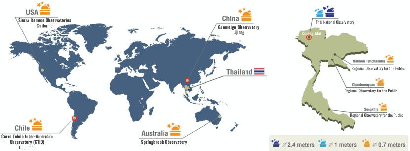
Figure 1: The location and size of the telescopes currently within the SPEARNET network. Telescopes with a red circle are those used to take the observations of WASP-127 b discussed in Section 3.1. (Image credit: NARIT)

Table 1: Details of the SPEARNET observations of WASP-127 b, obtained using the Thai National Telescope (TNT), telescope from the Thai Robotic Telescope network at Gao Mei Gu (TRT-GAO), and the PROMPT-8 telescope at the Cerro Tololo Inter-American Observatory. Since the observations were taken, TRT-TNO has been upgraded to a $1$ m aperture telescope.

Date	Telescope	Filter	Aperture (m)	Number of photometric points	Exposure time (s)	Transit coverage
15-02-2017	TNT	$i^{\prime}$	$2.4$	24 720	0.78	Full
15-02-2017	TRT-GAO	$R$	$0.7$	1 223	15, 20	Full
21-03-2017	PROMPT-8	$R$	$0.6$	413	5	Egress only
26-02-2018	TNT	$r^{\prime}$	$2.4$	68 480	0.38	Full
09-03-2019	TNT	$u^{\prime}$	$2.4$	741	12.8	Ingress only
30-03-2019	TNT	$u^{\prime}$	$2.4$	1 531	12.8	Full

The images obtained by SPEARNET were calibrated using IRAF routines along with astrometric calibration using Astrometry.net (Lang et al., 2010). In order to obtain the light curve, aperture photometry was carried out using sextractor (Bertin & Arnouts, 1996) using an adaptive scaled aperture based on the seeing in an individual image. Reference stars were chosen to have magnitudes similar to WASP-127 ($\left|\Delta M\right|<3$) and no intrinsic variation. The observed time in BJD${}_{\textrm{TDB}}$ with flux ratio between WASP-127 b and reference stars with their error are shown in Table 2.

Table 2: The photometric data of WASP-127 b.

BJD${}_{\textrm{TDB}}$	Flux	Flux error	Filters	Telescopes
2 457 800.1182452	2.387	0.007	$i^{\prime}$	TNT
2 457 800.1182542	2.424	0.008	$i^{\prime}$	TNT
2 457 800.1182633	2.367	0.007	$i^{\prime}$	TNT
2 457 800.1182724	2.394	0.008	$i^{\prime}$	TNT
2 457 800.1182815	2.379	0.007	$i^{\prime}$	TNT
2 457 800.1182905	2.358	0.007	$i^{\prime}$	TNT
2 457 800.1182996	2.414	0.008	$i^{\prime}$	TNT
2 457 800.1183087	2.430	0.008	$i^{\prime}$	TNT
2 457 800.1183178	2.408	0.007	$i^{\prime}$	TNT
⋮	⋮	⋮	⋮	⋮

Note. The raw lightcurves are available at the CDS.

The obtained light curves, shown in 2(a), were then run through TransitFit, using the ‘batched’ mode, a 2nd-order detrending function, using quadratic limb-darkening model, and both ‘coupled’ and ‘independent’ LDC fitting approaches so as to able to identify the improvement from using filter and host parameters to inform the likelihood of LDC values. For the coupled LDC approach, we adopted the stellar parameters of Lam et al. (2017), namely $T=5620\pm 85$ K, $R_{\star}=1.39\pm 0.03~{}R_{\odot}$, $M_{\star}=1.08\pm 0.03~{}M_{\odot}$, $\log g=4.18\pm 0.01$ cgs, and [Fe/H] $=-0.18\pm 0.06$ dex. For the priors, we take the values from Chen et al. (2018). The value of $t_{0}$ was scaled using $P$ to match the time span of the raw lightcurves, to reduce extrapolation during fitting.

The resulting detrended light curves from the coupled LDC fitting are shown with the best-fit model in Figure 2(b). The corresponding corner plot showing posteriors are shown in Figure 10 in Appendix A. We also show the resulting transit depths from both the coupled and independent LDC mode retrievals alongside the Hubble Space Telescope (HST) spectrum from Skaf et al. (2020), and the Gran Teliscopio Canarais (GTC) and Nordic Optical Telescope (NOT) spectral data and best fit model from Chen et al. (2018) in Figure 3.

Since our data, and those of Chen et al. (2018) and Skaf et al. (2020) have all been analysed separately, there is an intrinsic offset between all the data. We have compared the data with our retrieved spectrum in Figure 3. The wavelength positions of the SPEARNET observations in Figure 3 are derived by weighting the relevant filter profile by the spectral energy distribution (SED) of WASP-127, predicted using the PHOENIX models.

Looking at Figure 3, from coupled LDC fitting approach, the value of $R_{p}/R_{\star}$ is somewhat different than the independent LDC fitting method, with a discrepancy of around $8$ per cent in the $u^{\prime}$ and $r$ bands. This difference is larger than the $3$ per cent bias that Espinoza & Jordán (2015) find can be introduced from not fitting LDCs at all, and clearly illustrates the impact that using host characteristics and filter profiles can have when fitting spectroscopic and photometric measurements.

This could also be due to the incompleteness of the observation, as in the case of $R$-band and $u^{\prime}$-band, which do not have a complete transit observed. When using the coupled LDC approach, the fact that this observation does not have a complete transit may have an effect on the parameters retrieved for all the filters. Table 3 shows the physical results obtained by each of the two retrievals described above.

Looking at Figure 3, it may be noticed that the transit depth precision obtained from the TNT observations are roughly comparable to those obtained by Skaf et al. (2020) from their HST observations. At first glance, this may appear surprising, as one would instinctively expect that space-based observations would produce higher-quality results than those made from ground-based observatories. However, this fails to account for the impact of the high on-sky efficiency of observations made using ULTRASPEC as well as the difference between broadband imaging and spectroscopy. Assuming that calculations are photon-noise limited, we expect the signal-to-noise ratio (S/N) on the retrieved flux value to go as $\sqrt{N_{\gamma}}$, where $N_{\gamma}$ is the number of photons collected. Using this, S/N for the transit depth can be estimated by $\sqrt{N_{\gamma,\textrm{t}_{14}}+N_{\gamma,\textrm{base}}}$ where $N_{\gamma,\textrm{t}_{14}}$ and $N_{\gamma,\textrm{base}}$ are the number of photons in-transit and in baseline respectively. In the source-dominated limit $N_{\gamma}$ can be estimated by

$$N_{\gamma}=t_{\textrm{int}}10^{-0.4\left(m-m_{0}\right)},$$ (26)

where $t_{\textrm{int}}$ is the on-sky integration time, $m$ is the host apparent magnitude and $m_{0}$ the instrument zero-point magnitude.

For TNT in $r^{\prime}$ the zero-point magnitude is $m_{0,{\rm TNT}}=25.25$ and with 42,680 in-transit observations with a mean exposure of 0.38 s this gives $N_{\gamma,\text{t}_{14},\text{TNT}}\simeq 1.7\times 10^{10}$ integrated over all in-transit exposures of WASP-127 ($r^{\prime}=10.0$). With 26,088 baseline observations, we also get $N_{\gamma,\text{base},\text{TNT}}\simeq 1.0\times 10^{10}$.

Skaf et al. (2020) observed 38 in-transit observations using the HST Wide Field Camera 3 (WFC3) G141 grism with a mean exposure of 95.782 s. Using the WFC3IR spectroscopic exposure time calculator, and adopting a G5V host spectrum for WASP-127 normalised to $V=10.15$ mag, we find a photon count integrated over all in-transit exposures of $N_{\gamma,\text{t}_{14},\text{HST}}\simeq 3.4\times 10^{9}$ at 1.4 $\mu$m for a spectral resolution of 70. The corresponding baseline count gives us $N_{\gamma,\text{base},\text{HST}}\simeq 3.2\times 10^{9}$. This gives a rough ratio of S/N for TNT to S/N for HST, of

$$\sqrt{\frac{N_{\gamma,\text{t}_{14},\text{TNT}}+N_{\gamma,\text{base},\text{TNT}}}{N_{\gamma,\text{t}_{14},\text{HST}}+N_{\gamma,\text{base},\text{HST}}}}\simeq 4.2.$$

Clearly, the approximate equality here masks the fact that we are comparing the throughput of a broadband filter on TNT to the sensitivity of a single spectral bin from the G141 grism.

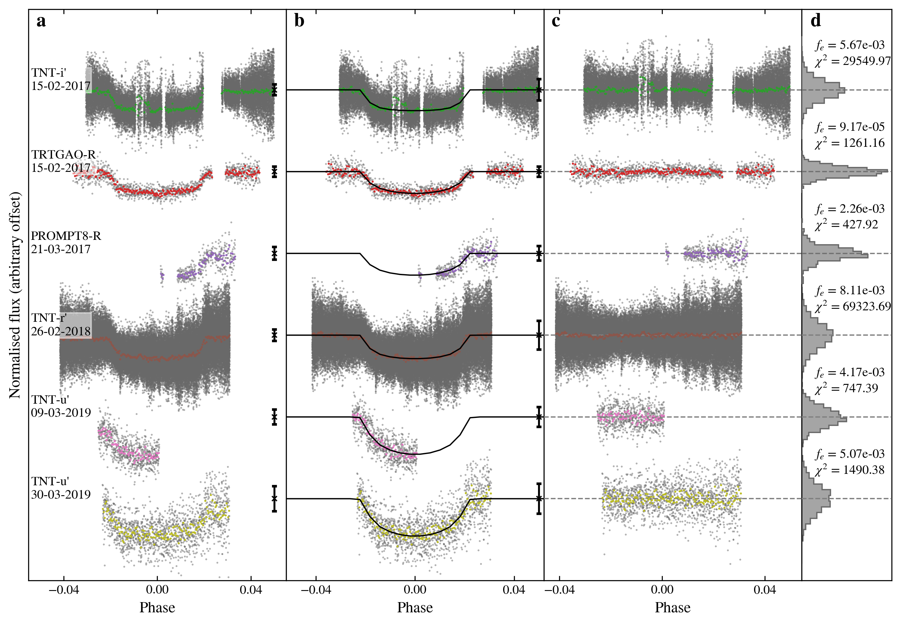
Figure 2: (a): The raw data from the SPEARNET observations of WASP-127 b outlined in Table 1, normalised using the median values for each observation and phase folded using the model obtained in (b). We have binned the observations to a 2-minute cadence, with the raw observations shown in grey. For clarity, error bars on data points have been excluded and an average error bar of the raw data points has been provided as a black coloured bar to the right of each curve. (b): The detrended light curves and associated best-fit models obtained using TransitFit in “batched” mode with a coupled quadratic LDC fitting and simultaneous normalisation and 2nd-order detrending. Each curve has an arbitrary offset from a normalised baseline of $1$ and has been phase-folded to centre $t_{0}$ at a phase of 0.0. The best fit transit model from the retrieval is over-plotted. We show the average of the errors scaled using retrieved value of $f_{e}$, as a black coloured point on the right of each curve. (c): The residuals after model is subtracted from the fitted lightcurves. (d): The histogram of the residuals along with the respective $\chi^{2}$ values.

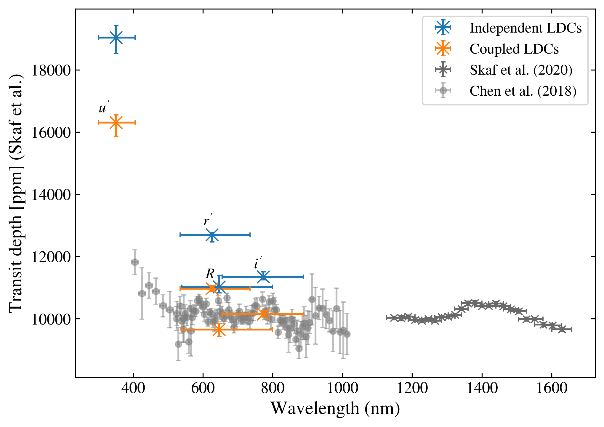
Figure 3: The transmission spectrum of WASP-127 b, obtained by fitting ground-based observations from the SPEARNET telescope network using TransitFit in coupled (orange) and independent (blue) LDC fitting modes with a second-order detrending function. From left to right the filters are $u^{\prime}$, $r^{\prime}$, $R$, and $i^{\prime}$, and we have labelled the independent LDC depths for quick reference. Also shown are the GTC/NOT observations (after applying corrective offset) reported in Chen et al. (2018, light grey) and the HST reported in Skaf et al. (2020, dark grey). For the SPEARNET data points, the horizontal positions and error bars are derived from the SED-weighted filter profiles, with the data point positioned at the weighted mean of each profile and the error bars reflecting the standard deviations. For the other data sources, horizontal error bars represent the complete bandwidth of each spectroscopic filter.

Table 3: Output parameters from using TransitFit to run retrieval on photometric observations of WASP-127b, in both coupled and independent LDC fitting mode. For comparison, we provide the orbital parameters obtained by Chen et al. (2018) and Skaf et al. (2020). We have converted the Chen et al. (2018) value of $a/R_{\star}$ into AU using the Lam et al. (2017) value of $R_{\star}=1.39\pm 0.03~{}R_{\odot}$.

	SPEARNET observations
	Coupled LDC fitting	Independent LDC fitting
$P$ [days]	$4.1780626^{+0.0000019}_{-0.0000026}$	$4.1780667^{+0.0000015}_{-0.0000019}$
[BJD${}_{\textrm{TDB}}$]	$2457800.24581^{+0.00016}_{-0.00018}$	$2457800.24543^{+0.00021}_{-0.00009}$
$i$ [deg]	$89.64^{+0.24}_{-0.20}$	$86.36^{+0.28}_{-0.12}$
$a/R_{\star}$	$7.837^{+0.026}_{-0.016}$	$7.333^{+0.117}_{-0.051}$
$a$ [AU]	$0.0507^{+0.0011}_{-0.0011}$	$0.0474^{+0.0013}_{-0.0011}$
$R_{p}/R_{\star}$ [$u^{\prime}$- band]	$0.1277^{+0.0010}_{-0.0017}$	$0.1380^{+0.0014}_{-0.0018}$
$R_{p}/R_{\star}$ [$r^{\prime}$- band]	$0.1047^{+0.0005}_{-0.0003}$	$0.1127^{+0.0003}_{-0.0010}$
$R_{p}/R_{\star}$ [$R$- band]	$0.0983^{+0.0010}_{-0.0011}$	$0.1050^{+0.0017}_{-0.0009}$
$R_{p}/R_{\star}$ [$i^{\prime}$- band]	$0.1007^{+0.0005}_{-0.0004}$	$0.1065^{+0.0008}_{-0.0004}$
$u_{0}$ [$u^{\prime}$-band]	$0.868^{+0.078}_{-0.036}$	$0.934^{+0.103}_{-0.147}$
$u_{1}$ [$u^{\prime}$-band]	$0.010^{+0.077}_{-0.029}$	$-0.446^{+0.191}_{-0.165}$
$u_{0}$ [$r^{\prime}$-band]	$0.534^{+0.023}_{-0.036}$	$0.709^{+0.034}_{-0.055}$
$u_{1}$ [$r^{\prime}$-band]	$0.363^{+0.033}_{-0.041}$	$-0.350^{+0.066}_{-0.063}$
$u_{0}$ [$R$-band]	$0.763^{+0.061}_{-0.042}$	$0.514^{+0.275}_{-0.154}$
$u_{1}$ [$R$-band]	$0.143^{+0.060}_{-0.039}$	$0.001^{+0.272}_{-0.131}$
$u_{0}$ [$i^{\prime}$-band]	$0.287^{+0.034}_{-0.026}$	$0.102^{+0.124}_{-0.053}$
$u_{1}$ [$i^{\prime}$-band]	$0.646^{+0.057}_{-0.041}$	$0.271^{+0.157}_{-0.139}$
	Chen et al. (2018)	Skaf et al. (2020)
$P$ [days]	$4.17807015\pm 5.7\times 10^{-7}$	$4.1780619\pm 1.3\times 10^{-6}$
$t_{0}$ [BJD${}_{\textrm{TDB}}$]	$2457248.741276\pm 0.000068$	$2458238.943367\pm 0.000055$
$i$ [deg]	$87.88\pm 0.32$	$88.2\pm 1.1$
$a/R_{\star}$	$7.846\pm 0.089$	$7.846~{}^{\textrm{a}}$
$a$ [AU]	$0.0507\pm 0.0012$	$0.0507~{}^{\textrm{a}}$
${}^{\textrm{a}}$ Skaf et al. (2020) adopt the value of $a/R_{\star}$ directly from Chen et al. (2018)

3.2 Multi-epoch study of WASP-91 b with TESS

WASP-91 b is a $1.34~{}M_{\text{Jup}}$ warm Jupiter with a 2.8 day orbit around a K3 host star (Anderson et al., 2017). With a radius of $1.03~{}R_{\text{Jup}}$, WASP-91 b is a smaller example of a hot Jupiter, and has not been the subject of further studies since its discovery.

TESS observed WASP-91 b in Sectors 1, 27, and 28, capturing a total of 50 158 photometric data points covering 26 transits, the data which we acquired from the Barbara A. Mikulski Archive for Space Telescopes (MAST) portal. We use 120 s cadence data, and PDC$\_$SAPFLUX values are taken as flux. Since these data contain vast numbers of observations outside of transit, and there are multiple offsets and other trends within the data which cannot be modelled with a simple polynomial, we estimate the transit duration $t_{14}$, assuming a circular orbit with a $90$ degree inclination, using

$$t_{14}=\frac{R_{p}+R_{\star}}{a\pi}P$$ (27)

and discard any data which are more than $2.5t_{14}$ away from the mid-transit times predicted by the ephemeris given in Anderson et al. (2017). This results in 26 transits, capturing a combined total of 9 789 photometric points, which can then be individually normalised and detrended with low-order polynomials. This splitting of data is provided in TransitFit through the split_lightcurve_file function.

After splitting the full data into individual transit observations, we use the “folded” mode of TransitFit to fit these data, using both the “coupled” and “independent” LDC fitting modes, assuming a circular orbit and using the quadratic limb-darkening model from Equation 2 and a second-order detrending polynomial. The values from Anderson et al. (2017) were used as priors for our fitting. For the “coupled” mode, we inform LDC fitting using the stellar parameters found by Anderson et al. (2017), given in Table 4, and the TESS filter profile given on by the SVO Filter Profile Service (Rodrigo et al., 2012; Rodrigo & Solano, 2020).

Figure 4 shows the fitting process for the “coupled” run of TransitFit at various stages. Figure 4 a(i) and a(ii) show the raw TESS observations which clearly exhibit various offsets and long-term trends. In order to reduce the impact of these, we split the data into individual transits using the approach described above, and Figure 4(b) shows the resulting raw data for the first transit. In the “folded” fitting mode, each transit is normalised and detrended, and Figure 4(c) shows the first transit after this first stage of processing. We have overplotted the final best fit model to help illustrate this step, but it should be noted that this model is calculated from all the transits, not just this single epoch. Once normalisation and detrending has been fitted for each transit, all the light curves are folded together and this curves is analysed to retrieve the final best-fit model. Figure 4(d) shows this folded light curve, along with the final best-fit transit model and residuals, which have an rms of 0.0017. We also show the same folded data binned to a cadence of two minutes, to demonstrate the improvement in observation precision when compared to the single-transit TESS observations like the one shown in Figure 4(c). An average of nearly $25$ photometric points are contained within each of the bins, which through naïve root-$N$ statistics suggests a maximum improvement in precision of factor $5$. The rms of the residuals of this binned light curve is 0.0004, which is an improvement of factor 4.8. The similarity of these two factors suggest that the improvement due to folding is near maximal, and thus the binned data are not systematics-limited.

We present the results from both runs of TransitFit alongside the results from Anderson et al. (2017) in Table 4, which are all consistent with each other. Precise ephemerides are required for accurate study of TTVs, and updating ephemeris by applying TransitFit to planets within TESS data will prove invaluable to future surveys.

The uncertainties on the two TransitFit retrievals are generally comparable, with the notable exception of the LDCs. Through using LDTk to calculate LDC likelihoods, we see upto an order-of-magnitude increase in the precision of LDC values, which demonstrates the impact of introducing host parameters and filter information into transit-fitting routines.

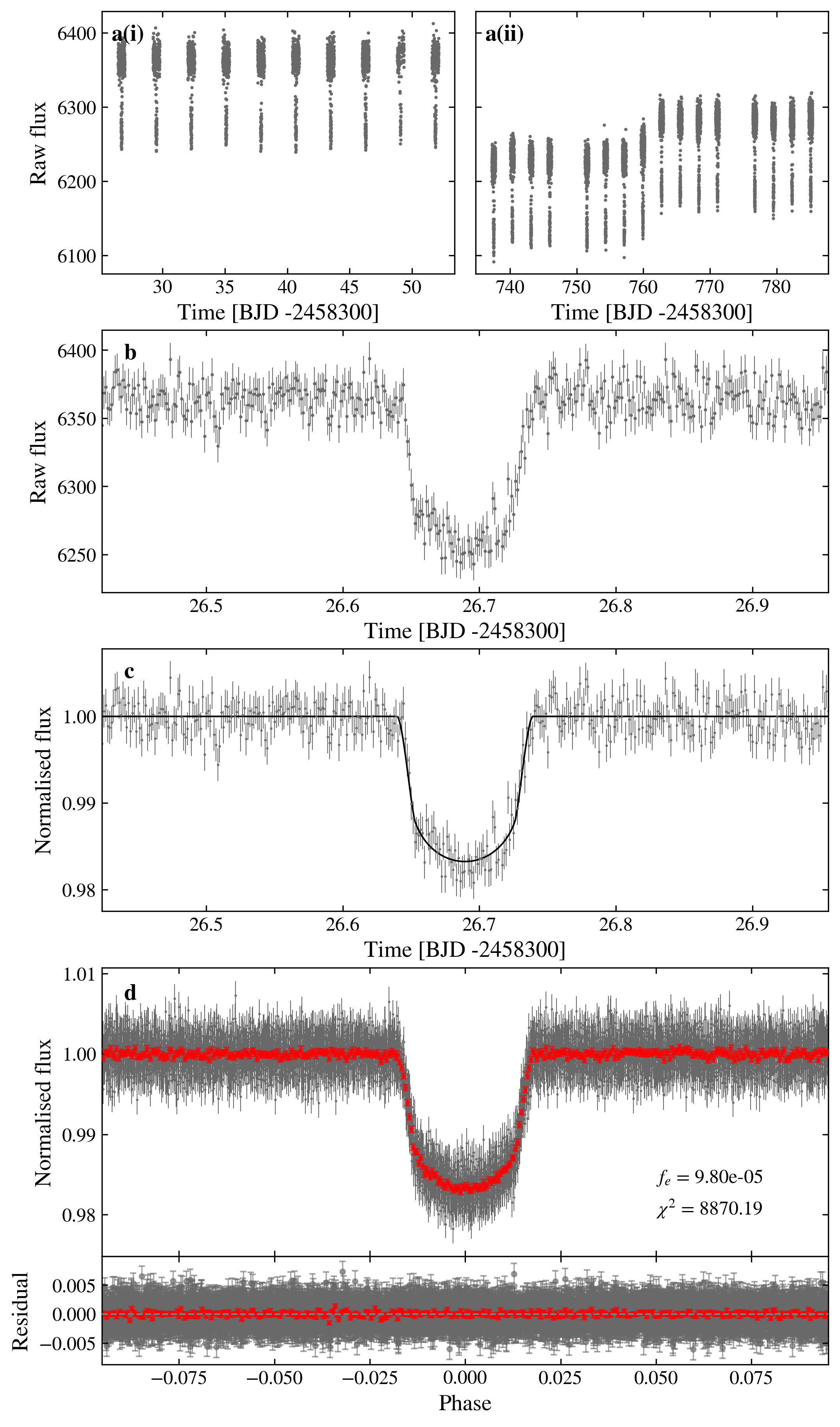
Figure 4: The full data processing of the TESS observations of WASP-91 b using the “folded” retrieval mode of TransitFit, with LDCs informed by LDTk. a(i): the raw observations from TESS Sector 1; a(ii): the raw observations from Sectors 27 and 28. We have excluded the error bars from these two plots for clarity; b: The raw data from the first observed transit, chosen purely as an illustration; c: The first observed transit after the first stage of “folded” mode retrieval. These data have been detrended and normalised, the error bars have been scaled using the retrieved $f_{e}$, and have the final best-fit model overplotted; d: the final phase-folded light curve, best-fit transit model and residuals, containing 9 789 photometric data points, and, in red, the same data binned to a 2 minute observation cadence. The error bars have been scaled using $f_{e}$, and the corresponding $\chi^{2}$ value has also been displayed.

Table 4: Output parameters for retrieval using TransitFit in “folded” retrieval mode on TESS observations of 26 transits of WASP-91 b, using both “coupled” and “uncoupled” LDC fitting approaches, alongside those obtained by Anderson et al. (2017). The data were fitted using a 2nd-order detrending model and the quadratic limb-darkening law given in Equation 2, and assuming zero orbital ellipticity, using the profile of the TESS filter available on the SVO Filter Profile Service to calculate LDC likelihoods when using LDTk. The TransitFit retrieval uses host parameters fixed at those obtained by Anderson et al. (2017), which are used in tandem with the filter profile to inform the LDC likelihood fitting.

	TransitFit: coupled LDCs	TransitFit: independent LDCs	Anderson et al. (2017)
$P$ [days]	$2.7985783^{+0.0000024}_{-0.0000027}$	$2.7985794^{+0.0000021}_{-0.0000020}$	$2.798581\pm 3\times 10^{-6}$
$t_{0}$ [BJD${}_{\textrm{TDB}}$]	$2458326.6895^{+0.0006}_{-0.0004}$	$2458326.6894^{+0.0005}_{-0.0005}$	$2456297.7190\pm 0.0002$ ${}^{\textrm{a}}$
$i$ [deg]	$87.36^{+0.20}_{-0.17}$	$87.21^{+0.31}_{-0.17}$	$86.8\pm 0.4$
$a/R_{\star}$	$9.34^{+0.12}_{-0.11}$	$9.28^{+0.16}_{-0.10}$	$9.251\pm 0.408$
$a$ [AU]	$0.0374^{+0.0014}_{-0.0014}$	$0.0371^{+0.0014}_{-0.0014}$	$0.037\pm 0.001$
$R_{p}/R_{\star}$	$0.1198^{+0.0005}_{-0.0005}$	$0.1206^{+0.0008}_{-0.0013}$	$0.1225\pm 0.0012$
$R_{p}$ [$R_{\text{Jup}}$]	$1.002^{+0.039}_{-0.031}$	$1.009^{+0.042}_{-0.024}$	$1.03\pm 0.04$
$u_{0}$	$0.505^{+0.021}_{-0.031}$	$0.551^{+0.137}_{-0.210}$	- ${}^{\textrm{b}}$
$u_{1}$	$0.121^{+0.021}_{-0.031}$	$0.016^{+0.090}_{-0.203}$	- ${}^{\textrm{b}}$
$T_{\text{eff},\star}$ [K]	-	-	$4920\pm 80$
$M_{\star}$ [$M_{\odot}$]	-	-	$0.84\pm 0.07$
$R_{\star}$ [$R_{\odot}$]	-	-	$0.86\pm 0.03$
[Fe/H]	-	-	$0.19\pm 0.13$
${}^{\textrm{a}}$ The time standard is not specified   .
${}^{\textrm{b}}$ Anderson et al. (2017) use the non-linear limb-darkening law but do not provide coefficients to compare with.

3.3 TTV analysis of WASP-126 b

Orbiting a type G2 star with a period of $3.2888\pm 0.0008$ days, WASP-126 b (Maxted et al., 2016) is a $0.28\pm 0.04~{}M_{\text{Jup}}$ hot Jupiter which has been identified as potentially exhibiting TTVs. Through Bayesian $N$-body simulation coupled with machine learning analysis of Sectors 1–3 of the TESS observations of WASP-126 b, Pearson (2019) showed that there was evidence of a TTV signal with amplitude of $\sim 1$ minute and a period of $\sim 25$ days, which could be attributed to a non-transiting planet with $M_{p}=0.202\pm 0.077~{}M_{\text{Jup}}$ on a $7.63\pm 0.17$ day orbit, dubbed WASP-126 c. Maciejewski (2020) studied the TESS observations from sectors 1–13 and found that when the extra sectors were included, the TTV signal was not present at a statistically significant level.

Here we use the ability of TransitFit to account for TTVs to analyse the TESS observations of WASP-126 b from sectors 1–13, 27–34, 36–39, 61, and 63 to further investigate the presence of TTVs within these data, and to produce the most up-to-date values for the planetary and orbital parameters of WASP-126 b. As with the analysis of WASP-91 b, we use PDC$\_$SAPFLUX values for flux, and we discard all data that is more than $2.5t_{14}$ from the mid-transit times predicted by Maxted et al. (2016), which gives 180 individual transits. We then run analysis using TransitFit in both “coupled” and “independent” LDC fitting modes, using the quadratic limb-darkening law, a 2nd order detrending polynomial, assuming a circular orbit, and using results from Maxted et al. (2016) as priors. When using LDTk to calculate LDC likelihoods, we use the host parameters given in Maxted et al. (2016), which are presented in Table 5, and the TESS filter profile from the SVO Filter Profile Service. As discussed in Section 2.3, we first run analysis of the data assuming that there are no TTVs, and we use these results to provide priors to parameterise the ephemeris for the analysis where we allow for the presence of TTVs. Since TransitFit requires a fixed period to be provided when considering TTVs, this step should always be used to ensure complete consistency of results. The priors used in this initial step are based on the ephemeris of Maxted et al. (2016). The resulting ephemerides from this initial analysis are given in Table 5, and we use these results when allowing for the presence of TTVs, fixing the period at the values given and using the retrieved $t_{0}$ values as the mean of a Gaussian prior with a width of $0.007$ days.

The orbital parameters of WASP-126 b retrieved by TransitFit when allowing for TTVs are given in Table 5, for both “coupled” and “independent” LDC fitting modes. We present these alongside the results of Pearson (2019), Maciejewski (2020), and Maxted et al. (2016) for comparison. We find that the results from both runs are generally consistent but, as in the WASP-91 b analysis, the uncertainties on the LDCs for the “coupled” run are smaller.

We present the O-C plots for both modes of the TransitFit analysis in the left plots of Figure 5, with the associated Lomb-Scargle periodograms on the right. The top row are the results for the “coupled” LDC run, and the bottom row are the results for “independent” LDCs. The solid horizontal lines on the Lomb-Scargle periodograms represent the false alarm probabilities of 10, 5, and 1 per cent from bottom to top, calculated using astropy routines (Astropy Collaboration et al., 2013, 2018). For the “independent” LDCs, the O-C plot has a reduced chi-squared value of $\chi_{R}=$0.87, whilst the “coupled” LDC O-C gives $\chi_{R}=$0.85. We find that there are no periodicities of statistical significance within the O-C data for either the “coupled” or “independent” LDC runs, and consequently conclude that there is no evidence of TTVs that would be indicative of a second planet in the WASP-126 system, in agreement with the findings of Maciejewski (2020).

The approach to fitting taken by TransitFit differs to both Pearson (2019) and Maciejewski (2020), and consequently this result can be taken to be an independent verification of the findings of Maciejewski (2020). Pearson (2019) uses a simultaneous 2nd order detrending polynomial but this is is not explicitly constructed to be depth-conserving. They do, however, use LDTk in their handling of LDCs, but not to directly inform the likelihood of trial parameters. Instead, Pearson (2019) uses LDTk to find the highest likelihood LDC values for the host parameters and TESS filter and fixes the values here. We note however that the host parameters used by Pearson (2019) for this do not exactly match those of (Maxted et al., 2016), as indicated in Table 5, and it is unclear where the alternative value of host metallicity originates from.

Maciejewski (2020) fit physical parameters to the light curves after independently detrending the raw data. We note that they freely fit the LDCs without using the Kipping (2013) parameterisation built into TransitFit, and do not use any host information to inform the likelihoods. This is reflected in the larger LDC uncertainties. Maciejewski (2020) compares their final LDC values to those predicted by bi-linearly interpolating the LDC tables provided by Claret & Bloemen (2011) for the Cousins R and I bands and the Sloan Digital Sky Survey z band and then averaging the results to approximate the TESS filter, which suggests values of $u_{0}=0.30$ and $u_{1}=0.28$. These predicted values are closer to the results of the TransitFit “independent” LDC run, which most closely resembles the approach of Maciejewski (2020), but are in significant tension with the results from the “coupled” LDC run.

We therefore conclude that, by taking a different approach to the investigations of both Pearson (2019) and Maciejewski (2020), we have been able to independently verify the result of Maciejewski (2020) and find no statistically significant TTV signatures and, consequently, no evidence of a second planet in the WASP-126 b system.

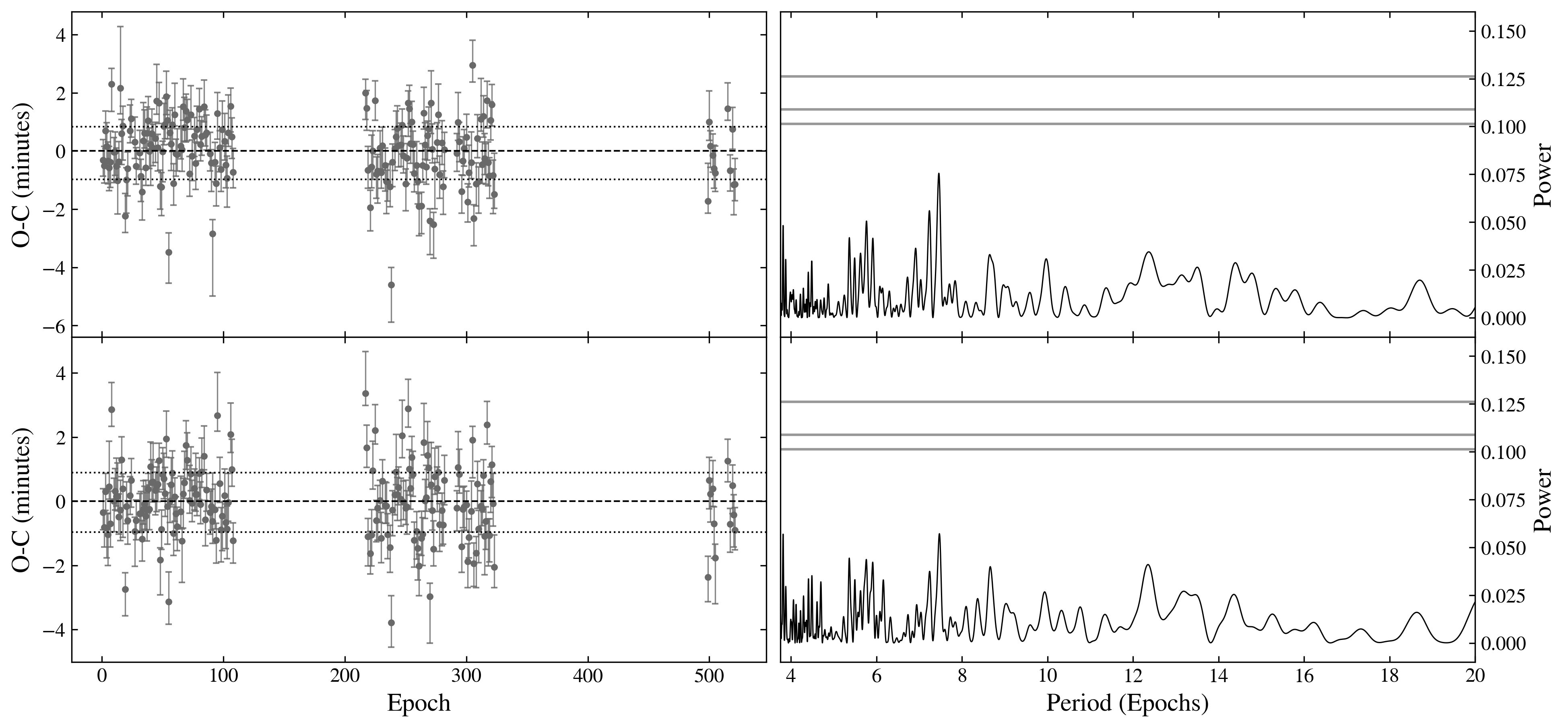
Figure 5: Left: The O-C plots of 126 transits of WASP-126 b observed by TESS, obtained from results of using TransitFit in “coupled” (top) and “independent” (bottom) LDC modes whist allowing for the presence of TTVs. The values of $t_{0}$ in this case had a median error of 4.97$\times 10^{-4}$ in the coupled mode and 4.90$\times 10^{-4}$ in the independent mode. The dotted lines represent the uncertainty on the predicted ephemerides derived from using TransitFit without allowing for TTVs. Right: The associated weighted Lomb-Scargle periodograms for each of the O-C plots. The horizontal grey lines represent the false alarm probabilities of $10$, $5$, and $1$ per cent from bottom to top.

Table 5: The planetary and orbital parameters of WASP-126 b derived using TransitFit in both “coupled” and “independent” LDC fitting modes on observations from sectors 1–13, 27–-34, 36–-39, 61, and 63 of the TESS mission. We present these alongside the values found by Pearson (2019), Maciejewski (2020), and Maxted et al. (2016). All fits assume zero orbital ellipticity, use a quadratic limb-darkening model, and unless otherwise stated assume the same host parameters as given by Maxted et al. (2016). A total of 94,021 datapoints were fitted, and it gave a value of $f_{e}=1.17\times 10^{-04}$ and $\chi^{2}=89,956.47$ for the “coupled" mode; and $f_{e}=1.21\times 10^{-04}$ and $\chi^{2}=89,898.40$ for the “independent" mode.

	TransitFit: coupled LDCs	TransitFit: independent LDCs	Pearson (2019)	Maciejewski (2020)	Maxted et al. (2016)
$P$ [days]	$3.2887859^{+0.0000036}_{-0.0000035}~{}^{\textrm{a}}$	$3.2887865^{+0.0000035}_{-0.0000039}~{}^{\textrm{a}}$	$3.2888\pm 1.94\times 10^{-5}$	- ${}^{\textrm{c}}$	$3.28880\pm 0.00001$
$t_{0}$ [BJD${}_{\textrm{TDB}}$]	$2458327.52083^{+0.00058}_{-0.00068}~{}^{\textrm{a}}$	$2458327.52070^{+0.00062}_{-0.00067}~{}^{\textrm{a}}$	-	$2456890.32004\pm 0.00061$	$2456890.3191\pm 0.0006$ ${}^{\textrm{d}}$
$R_{p}/R_{\star}$	$0.0776^{+0.0002}_{-0.0002}$	$0.0778^{+0.0002}_{-0.0003}$	$0.0783\pm 0.0002$	$0.07712^{+0.00063}_{-0.00047}$	$0.0781^{+0.0013}_{-0.0013}$
$R_{p}$ [$R_{\text{Jup}}$]	$0.959^{+0.078}_{-0.073}$	$0.962^{+0.079}_{-0.072}$	$0.964\pm 0.076$	$0.953\pm 0.075$	$0.965\pm 0.077$
$a/R_{\star}$	$7.771^{+0.099}_{-0.087}$	$7.719^{+0.107}_{-0.082}$	$7.887\pm 0.040$	$7.80^{+0.11}_{-0.20}$	$7.63^{+0.64}_{-0.23}$
$a$ [AU]	$0.0459^{+0.0037}_{-0.0037}$	$0.0456^{+0.0036}_{-0.0036}$	$0.0466\pm 0.0037$	$0.0461\pm 0.0038$	$0.0451\pm 0.0052$
$i$ [deg]	$88.53^{+0.60}_{-0.39}$	$88.27^{+0.57}_{-0.34}$	$89.51\pm 0.44$	$88.7^{+0.9}_{-0.9}$	$87.9^{+1.5}_{-1.5}$
$u_{0}$	$0.366^{+0.017}_{-0.023}$	$0.332^{+0.052}_{-0.028}$	$0.43~{}^{\textrm{b}}$	$0.32^{+0.07}_{-0.07}$	-
$u_{1}$	$0.193^{+0.026}_{-0.026}$	$0.229^{+0.069}_{-0.050}$	$0.14~{}^{\textrm{b}}$	$0.25^{+0.12}_{-0.13}$	-
$T_{\text{eff},\star}$ [K]	-	-	-	-	$5800\pm 100$
$M_{\star}$ [$M_{\odot}$]	-	-	-	-	$1.12\pm 0.06$
$R_{\star}$ [$R_{\odot}$]	-	-	-	-	$1.27\pm 0.08$
[Fe/H]	-	-	$-0.06$	-	$0.17\pm 0.08$
${}^{\textrm{a}}$ These values were derived assuming that no TTVs were present.
${}^{\textrm{b}}$ These values are those predicted by LDTk, using host parameters from Maxted et al. (2016) with $\textrm{[Fe/H]}=-0.06$.
${}^{\textrm{c}}$ The value of $P=2.8493819\pm 0.0000013$ days provided in Maciejewski (2020) appears to be a typo as it exactly matches the period given for WASP-100 b.
${}^{\textrm{d}}$ The time standard is not specified.

3.4 HST observations of WASP-43 b

WASP-43 b, discovered by Hellier et al. (2011), is a $2.034\pm 0.052~{}M_{\text{Jup}}$ hot Jupiter with a radius of $1.036\pm 0.019~{}R_{\text{Jup}}$, orbiting a type K7V star with a period of $0.813$ days (Gillon et al., 2012). The proximity of the planet to the host star makes it an ideal candidate for emission spectroscopy, and it is one of the few exoplanets to have observed emission phase curve data (Stevenson et al., 2014). Other studies have shown that WASP-43 b possesses a strong day-night temperature contrast (Stevenson et al., 2014; Gandhi & Madhusudhan, 2018) and consequently strong equatorial jets in the atmosphere (Kataria et al., 2016).

Since the first detection of an atmosphere by Murgas et al. (2014), multiple transmission spectroscopy studies have been completed, with detections including water (Kreidberg et al., 2014), carbon monoxide, carbon dioxide (Feng et al., 2016), aluminium oxide (Chubb et al., 2020), and multiple hydrocarbon hazes (Helling et al., 2020). Emission spectroscopy studies have also been utilised (Stevenson et al., 2014; Kreidberg et al., 2014; Blecic et al., 2014; Stevenson et al., 2017), and from these it has become apparent that a difference in the abundance of water exists between the day and night sides of the planet.

Several of these studies, including those of Tsiaras et al. (2018) and Chubb et al. (2020), make use of the Kreidberg et al. (2014) observations from HST, taken as part of observing program $13467$ (Bean, 2013). These observations were taken using the WFC3 G141 grism over the wavelength range of $1.135$–$1.642~{}\mu$m, and include three full-orbit phase curves, three primary transits, and two secondary eclipses. In this section, we demonstrate the application of TransitFit to the observations in the $1.135$–$1.158~{}\mu$m waveband. We limit ourselves to this single waveband in this paper, as we are using TransitFit to conduct an in depth study of observations of WASP-43 b from a wide range of sources (SPEARNET, in prep).

The observations which include a transit are shown in the top plot in Figure 6, normalised to a median value of 1. For the purposes of this discussion, we distinguish between visits and orbits. A visit is a single one of these observations, and can be directly translated to an epoch within TransitFit. Since HST is an orbital satellite, there are times during a visit where the source cannot be seen, which leads to a temporal striping effect. Each one of these stripes is referred to as an orbit. We also define $t_{\rm visit}$, the time elapsed since the first exposure in a visit and $t_{\rm orb}$, the time elapsed since the first exposure in an orbit.

It can clearly be seen that, in addition to the observation-long trends, there are two complex systematics which affect the observations. These are the alternating offset introduced by the upstream/downstream effect (McCullough & MacKenty, 2012), and ramp-up effects in observations made in each orbit (Berta et al., 2012; Agol et al., 2010). Following Kreidberg et al. (2018), we assume that the observed flux, $F_{\rm obs}$ is given by

$$F_{\rm obs}=F_{\rm sig}\times F_{\rm sys},$$ (28)

where $F_{\rm sig}$ is the astrophysical signal and $F_{\rm sys}$ is the signal from the systematics that need to be removed. We model these using

$$F_{\rm sys}=\left(S+v_{1}t_{\rm visit}+v_{2}t_{\rm visit}^{2}\right)\left(1-e^{-at_{\rm orb}-b}\right),$$ (29)

where

$$S=\begin{cases}1&\textrm{ for forward scans}\\ s&\textrm{ for reverse scans}\end{cases}$$ (30)

and $s$, $v_{1}$, $v_{2}$, $a$, and $b$ are all detrending coefficients. We note that Kreidberg et al. (2018) multiply $S$ by a normalisation coefficient, but we exclude this as it would be degenerate with the normalisation constant fitted by TransitFit.

Implementing the detrending model in Equation 29 as a custom detrending model within TransitFit, we analyse the observations using the folded mode , “coupled” LDCs, and priors centred around (Kreidberg et al., 2014) results. The phase-folded lightcurve, residuals, and binned residuals are shown in the bottom plot in Figure 6, where it is clear that the systematics have been removed. In Table 6 we give the retrieved orbital parameters alongside those of Kreidberg et al. (2014). The temporal results are broadly consistent, but there is a discrepancy between the retrieved values of $a$ and $R_{p}$. We suggest that this could be caused by the slightly different approach used by Kreidberg et al. (2014). The Kreidberg et al. (2014) detrending model is similar to our Equation (29), but excludes the quadratic $v_{2}t_{\rm visit}^{2}$ term from the visit-long trend, and it is not fitted simultaneously with their transit model. Additionally, there are only two free parameters used in the Kreidberg et al. (2014) transit model; $R_{p}/R_{\star}$ and a linear LDC. Their period is fixed to that of Blecic et al. (2014), whilst their values for $i$, $a$, and $t_{0}$ are determined by fitting white-light observations. In our analysis all of the transit and de-trending parameters are fitted simultaneously by TransitFit. Further investigation into these effects are being made as part of the aforementioned SPEARNET study, but we have included this section to demonstrate that TransitFit is capable of fitting light curves that exhibit systematics as complex as those seen in observations made by HST.

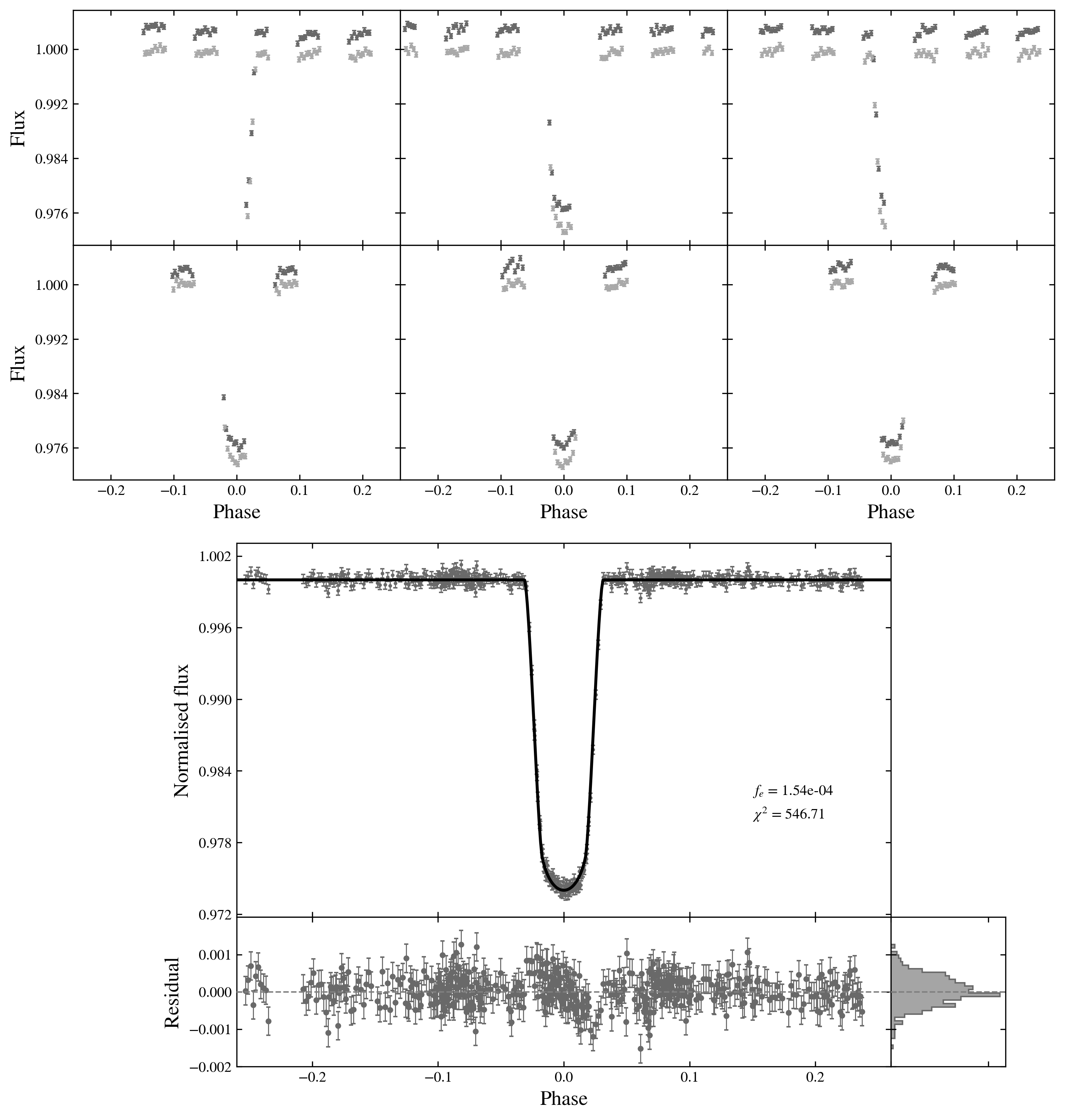
Figure 6: Top: Observations of six transits of WASP-43 b taken using the Wide Field Camera 3 (WFC3) on HST by Kreidberg et al. (2014). These data were all obtained using the $1.135$–$1.158~{}\mu$m waveband of the WFC3 G141 grism. The data from the first orbit of each visit and the first exposure of each orbit have been discarded and are not displayed or used in the subsequent analysis. The data are displayed here in raw form, normalised to a median value of $1$ and phase folded using the TransitFit-retrieved ephemeris given in Table 6. The scan direction used when obtaining the data introduces a systematic offset between the forward scan data (in dark grey) and the reverse scan data (in light grey). Bottom: The phase-folded light fitted curve obtained from the above data using TransitFit with a wavelength-coupled, quadratic limb darkening law and the custom detrending function given in Equation 29. The error bars have been scaled using the retrieved value of $f_{e}$. The best-fit light curve is over-plotted in black and the residuals are also displayed. We also report the $\chi^{2}$ corresponding to the fitting for a total of 469 datapoints.

Table 6: The orbital and planetary parameters of WASP-43 b obtained by TransitFit using the folded mode and wavelength-coupled quadratic LDC fitting on $1.135$–$1.158~{}\mu$m HST observations, alongside the values used and obtained by Kreidberg et al. (2014). The only free parameters in the Kreidberg et al. (2014) model are $R_{p}/R_{\star}$ and a linear LDC, the final value of which is not quoted.

	TransitFit	Kreidberg et al. (2014)
$P$ [days]	$0.81348^{+0.00006}_{-0.00015}$	$0.81347436$
$t_{0}$ [BJD${}_{\textrm{TDB}}$]	$2456601.0272^{+0.0020}_{-0.0005}$	$2456601.02748$
$R_{p}/R_{\star}$	$0.15764^{+0.00050}_{-0.00037}$	$0.1597\pm 0.0002$
$a/R_{\star}$	$4.951^{+0.026}_{-0.034}$	$4.872$
$a$ [AU]	$0.014^{+0.001}_{-0.001}$	-
$i$ [deg]	$82.44^{+0.01}_{-0.76}$	$82.1$
$u_{0}$	$0.242^{+0.025}_{-0.063}$	-
$u_{1}$	$0.221^{+0.061}_{-0.086}$	-

3.5 Combined fitting of JWST and HST observations of WASP-96 b

WASP-96 b is a hot Jupiter with a radius of $1.20\pm 0.06~{}R_{\text{Jup}}$ and mass of $0.48\pm 0.03~{}M_{\text{Jup}}$ orbiting a G8 type star with a period of $3.4$ days (Hellier et al., 2014). It has been a target for several atmospheric studies. An analysis of VLT FORS2 observations by Nikolov et al. (2018) showed an abundance of sodium in its atmosphere while predicting a cloud-free atmosphere at the limb. This analysis was reiterated in Nikolov et al. (2022) while confirming oxygen signatures in its atmosphere using HST WFC3 and Spitzer IRAC data. Further, McGruder et al. (2022) also confirmed that the WASP-96 b atmosphere showed minimal aerosol content at its terminator. However, Samra et al. (2022) has predicted a presence of a cloudy atmosphere following an analysis of VLT, Spitzer, and HST data. The atmosphere of WASP-96 b was shown to have features of water in its spectrum by Yip et al. (2020) using HST observations, while also inferring a lack of high NH₃ in its atmosphere. As part of Early Release Observations of the JWST, WASP-96 b was observed in NIRISS Single Object Slitless Spectroscopy (SOSS) mode consisting of 280 integration points, to demonstrate the capabilities of the instrument (Pontoppidan et al., 2022). In this section, we show the transmission spectrum of WASP-96 b generated from a TransitFit analysis applied simultaneously to this JWST data and to archive WFC3 HST data.

For the extraction of the lightcurves, the Stage 1 images from the NIRISS observations were processed following Feinstein et al. (2023) and JWST data analysis tools. The images were corrected for bad pixels identified by DQ flags, by replacing them with the median value of the 9x9 pixel grid centred on them. After applying a flat-field correction, we traced the order 1, order 2, and order 3 spectra. The trace was then smoothed out by fitting it with a Chebyshev polynomial. The spectra of all three orders were masked out within 20 pixels from their traces and a noise and background correction was applied by removing the column median of the residual image. The traces of the spectra and the background-corrected versions are shown in Figure 7. With an aperture radius of 15 pixels, we extracted lightcurves from order 1 in 850-2800 nm range and from order 2 spectra in 600-850 nm range only, leaving out the noisier order 3 spectrum. The wavelength integrated lightcurve of this spectrum had a median noise of 720.1 ppm as compared to 77.0 ppm for order 1 and 164.0 ppm for order 2. The lightcurves were binned in wavelength bins of 25 nm, using inverse variance weighting.

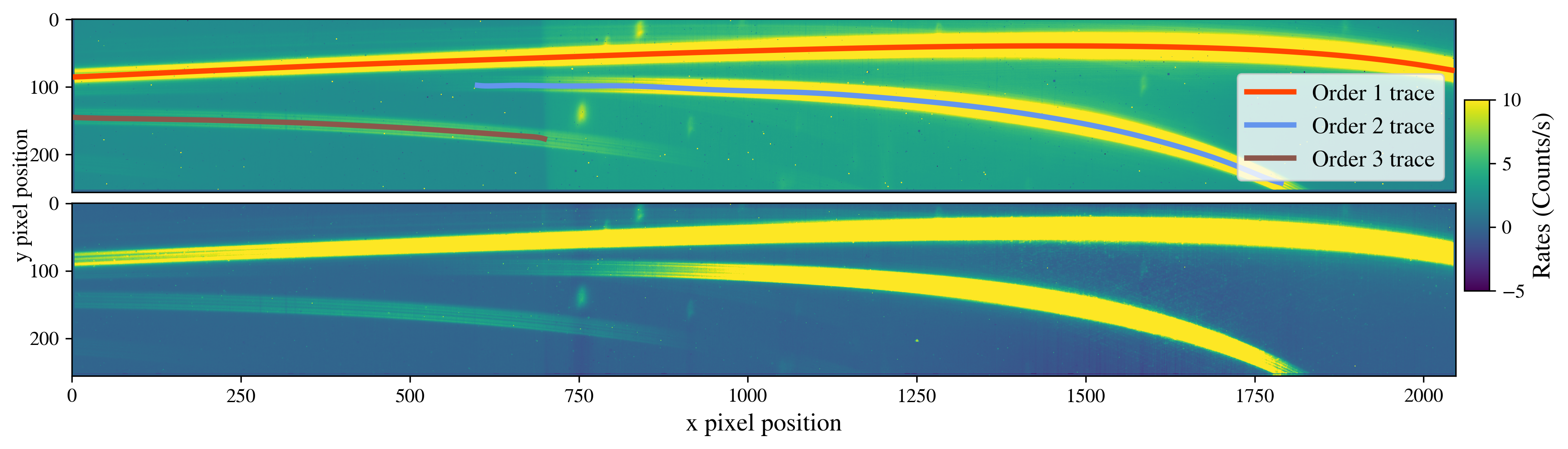
Figure 7: Top: The traced spectra for Order 1 (red), 2 (blue), and 3 (brown) of the GR700XD grism are shown overplotted on the median image from WASP-96 b observations. Bottom: The median of the image after noise correction.

HST data from G141 and G102 grisms were extracted using Iraclis (Tsiaras et al., 2016b; Tsiaras et al., 2016c) in bins similar to that of Yip et al. (2020). A total of 88 lightcurves obtained from JWST observations and 38 lightcurves from HST observations were fitted using TransitFit to generate a transmission spectrum. We use a 2nd-order detrending function for JWST lightcurves and a custom detrending function for HST lightcurves as with the analysis of WASP-43 b described in Section 3.4. The limb darkening coefficients were fitted in the coupled mode and using quadratic limb-darkening model. Planetary parameters and host parameters from Hellier et al. (2014) were used as priors and inputs, respectively, and are presented in Table 7. The “batched” mode was used for fitting these lightcurves, and the average of results weighted by inverse variance, were generated. Given the large number of lightcurves involved, there is a possibility of inter-batch variability in the wavelength-independent parameters. Consequently, the wavelength-dependent parameters might not result in the best-fit when used with the final results for wavelength-independent parameters. In order to reduce this discrepancy, we run the “batched” mode again. To generate priors for this run, we take the results from the first run, and calculate inverse variance weighted results from all batches leaving one batch at a time. The union of these results is taken as the prior for the wavelength-independent parameters in the second run, which gives us the final results.

Figure 8 shows the HST and JWST lightcurves after fitting , along with the best-fit model, with the best-fit values listed in Table 7, while the generated transmission spectrum is shown in Figure 9. The TransitFit spectrum appears to be in good agreement with the analysis of Yip et al. (2020).

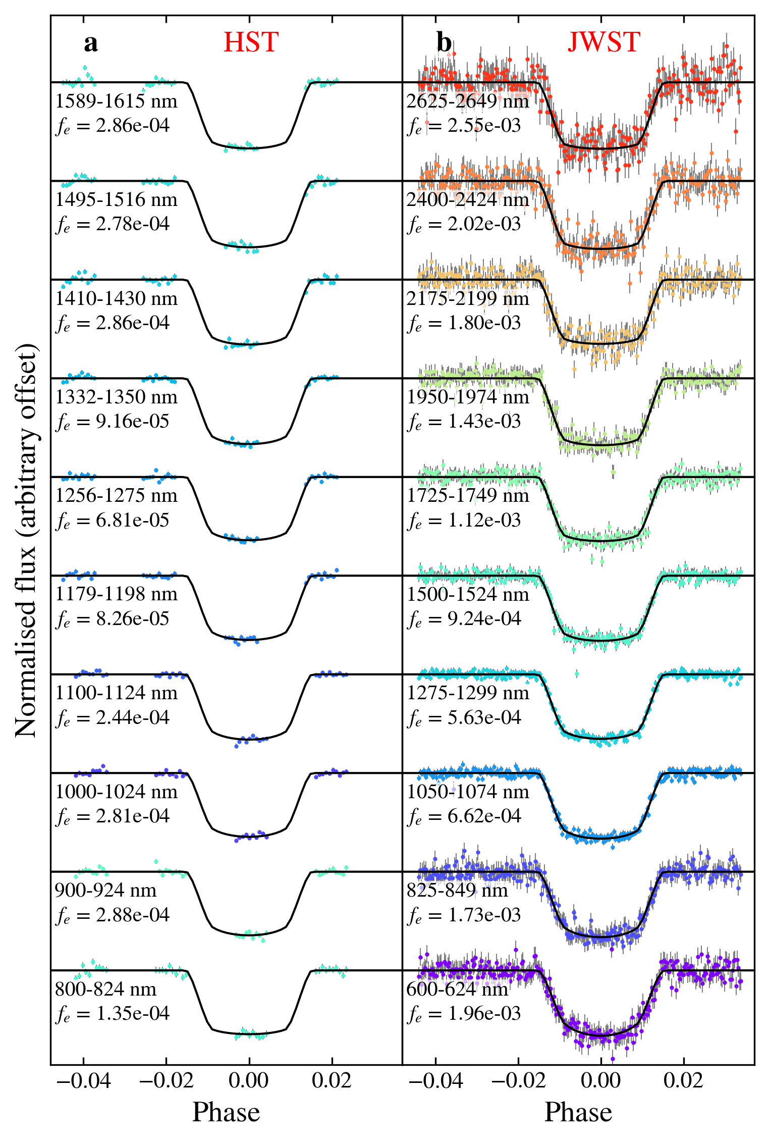
Figure 8: Left column (a): a sample of fitted lightcurves from HST observations of WASP-96 b, with the best-fit model overplotted in black. The error bars on all data points are plotted in grey and are scaled using the retrieved value of $f_{e}$. The corresponding wavelength bin for the lightcurves is indicated. The right column (b) shows the same for JWST data. TransitFit computed the best-fit model from both HST and JWST datasets simultaneously. The $\chi^{2}$ values for JWST lightcurves were in the range of 269.38- 294.91 with an average of 280.08. For HST lightcurves, the $\chi^{2}$ values were in the range of 38.07- 96.33 with an average of 53.89 for the data from G141 which had 44 data points. The data from G102 had 40 integration points and resulted $\chi^{2}$ values in the range of 38.46- 81.09 with an average of 59.22.

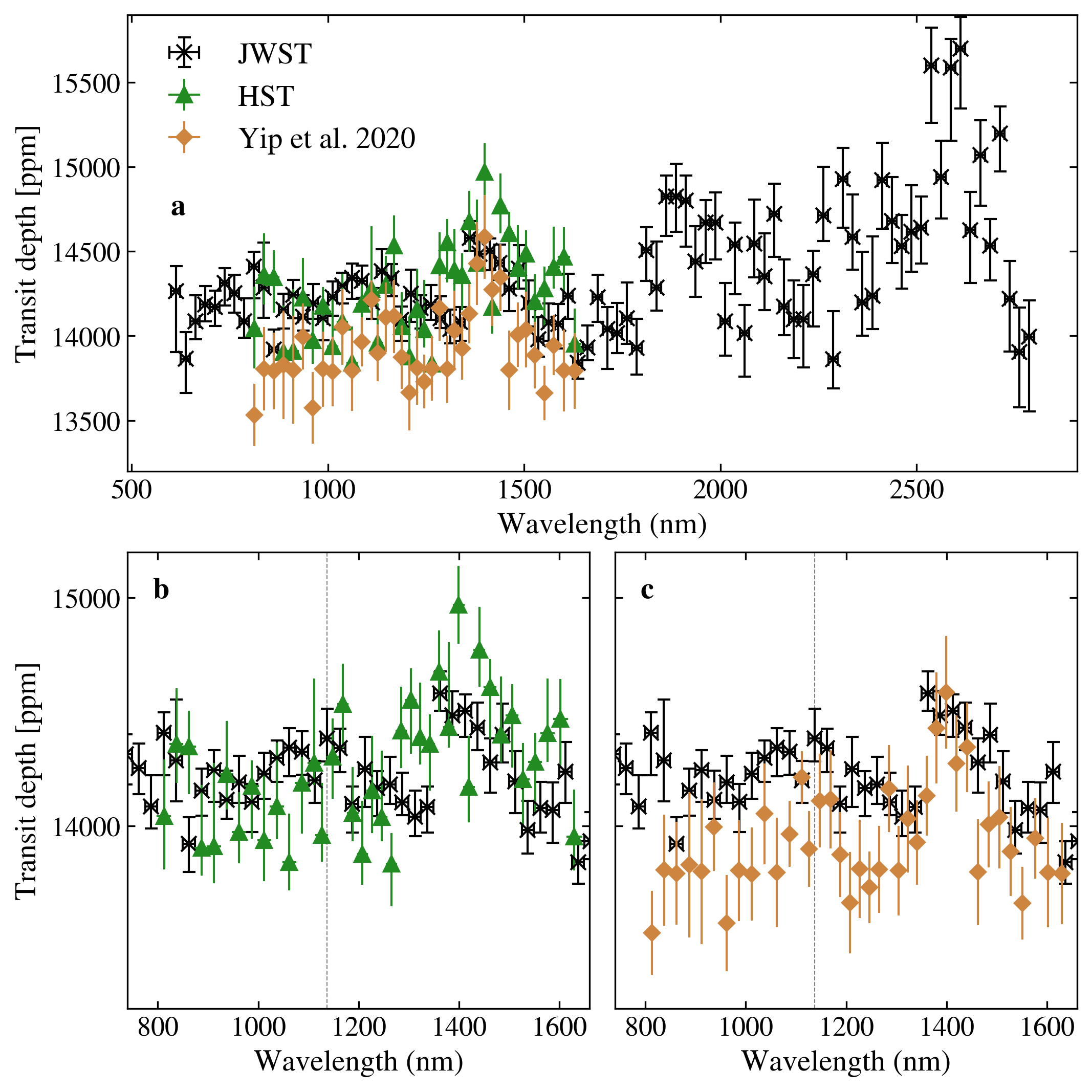
Figure 9: Top: TransitFit transmission spectrum of WASP-96 b derived simultaneously from JWST (black) and HST (green) observations. In orange, we also show for comparison the HST transmission spectrum obtained by Yip et al. (2020). Bottom: zoomed panels spanning the HST data range, showing the separate TransitFit (left) and Yip et al. (2020) (right) solutions. The vertical dotted lines in these lower panels separate the two epochs of HST observations.

Table 7: The planetary and orbital parameters of WASP-96 b derived using TransitFit analysis of the JWST mission. The values are compared with the values retrieved from Hellier et al. (2014), which were also used as priors for TransitFit.

	TransitFit	Hellier et al. (2014)
$P$ [days]	$3.4252519^{+0.0000011}_{-0.0000016}$	$3.4252602\pm 2.7\times 10^{-6}$
$t_{0}$ [BJD${}_{\textrm{TDB}}$]	$2458470.78034^{+0.00041}_{-0.00044}$	$2456258.0621\pm 0.0002$ ${}^{\textrm{a}}$
$a$ [AU]	$0.0441^{+0.0021}_{-0.0021}$	$0.0453\pm 0.0013$
$i$ [deg]	$85.422^{+0.019}_{-0.018}$	$85.6\pm 0.2$
$R_{p}$ [$\mathrm{R}_{\mathrm{J}}$]	-	$1.20\pm 0.06$
$T_{\text{eff},\star}$ [K]	-	$5500\pm 150$
$M_{\star}$ [$M_{\odot}$]	-	$1.06\pm 0.09$
$R_{\star}$ [$R_{\odot}$]	-	$1.05\pm 0.05$
[Fe/H]	-	$0.14\pm 0.19$
${}^{\textrm{a}}$ This value is in UTC. The corresponding prior for $t_{0}$ was
checked to be in-transit for the raw lightcurve.

4 Conclusions

We have presented TransitFit, a new open-source code for fitting exoplanetary transit light curves using nested sampling routines. TransitFit has been designed for transmission spectroscopy surveys employing multiple telescopes, and allows coupling of limb-darkening coefficients across observation wavelengths by utilising information on the host star and the LDTk Python package (Parviainen & Aigrain, 2015).

TransitFit has been developed in anticipation of a new “asset-starved” era of transmission spectroscopy studies, where limited observational time and resources mean that studies will frequently have to combine data of various quality, wavelength coverage, and sources. One such example of this is SPEARNET, a survey which is using a heterogeneous distributed network of small- to mid-sized ground-based telescopes to conduct atmospheric studies of transiting exoplanets.

Using TransitFit and observations from the SPEARNET telescope network, we have presented analysis of new data of the hot-Neptune WASP-127 b, which includes the first $u^{\prime}$-band observations of the planet. We have shown that introducing a wavelength-coupled approach to LDC fitting can result in changes as large as 8 per cent in the retrieved value of $R_{p}/R_{\star}$, or 17 per cent in measured transit depth.

We have demonstrated the application of TransitFit in more temporal-focused studies, analysing TESS observations of 26 transits of WASP-91 b to produce updated planetary ephemerides. This will prove invaluable in analysis of planets in the TESS catalogue, allowing for easy searches for TTV signatures. We have used TransitFit to analyse 180 transits of WASP-126 b observed by TESS and have found no statistically significant evidence for the presence of TTVs proposed by Pearson (2019).

We have also shown how TransitFit can be used in situations where observations display trends that cannot be adequately modelled with a low-order polynomial. We fitted observations of WASP-43 b from a single wavelength channel of HST and found that the complex systematics can be adequately removed. Further analysis of the full set of HST observations for WASP-43 b, in conjunction with observations from other telescopes, is being conducted as part of a separate study (SPEARNET, in prep). Moreover, we have already used TransitFit to analyse the combined ground-based, HST and TESS observations of HAT-P-26 b (A-thano et al., 2023). The analysis found the presence of TTVs and H₂O dominated atmosphere on the planets, which agrees with previous studies.

We used TransitFit to construct a combined transmission spectrum of WASP-96 b from simultaneous fitting of JWST NIRISS and HST WFC3 data. In general we found good correspondence between the HST and JWST datasets.

Data availability

The codes underlying TransitFit are available on GitHub at https://github.com/SPEARNET/TransitFit. The observational data of WASP-127 b obtained by SPEARNET and the TransitFit transmission spectrum of WASP-96 b can be downloaded at https://cdsarc.u-strasbg.fr/ftp/vizier.submit/transitfit_data/. TESS, JWST, and HST observations are publicly available from https://mast.stsci.edu.

Appendix A Posterior plots

TransitFit returns the best-fit parameters which are the samples from dynesty with highest likelihood. The fitting algorithm also generates posterior plots to show the density of parameters in the range of priors. A posterior plot is generated for each batch of fitting, and for the phase-pholded lightcurve if applicable. In Figure 10 we have shown a posterior plot for selected parameters corresponding to WASP-127 b fitting in ‘coupled’ mode.

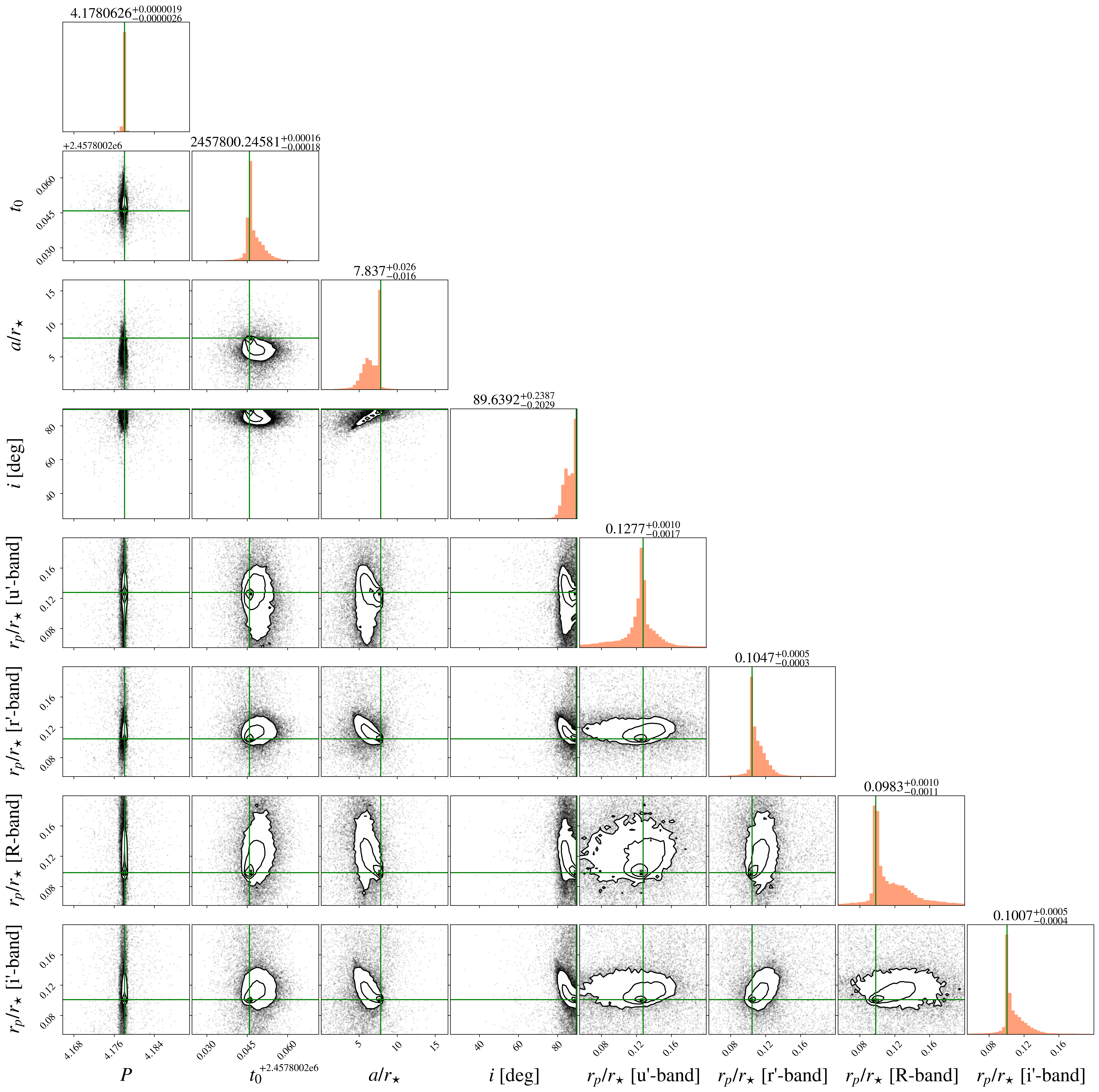
Figure 10: A posterior plot showing distribution of parameters samples across the range of priors. We use gaussian priors for $P$, $t_{0}$, and $a/r_{\star}$; and uniform priors for $R_{p}/R_{\star}$. The priors for inclination angle ($i$) are from a gaussian distribution clipped at a maximum of 90 degrees. These samples were taken for WASP-127 b fitting in ‘coupled’ mode, and are plotted without weights. The LDCs, normalisation factor, and detrending coefficients are not shown for simplicity. The best fit values and corresponding error limits are shown as the titles of histograms.

References

- A-thano et al. (2023) A-thano N., et al., 2023, arXiv e-prints, p. arXiv:2303.03610
- Agol et al. (2010) Agol E., Cowan N. B., Knutson H. A., Deming D., Steffen J. H., Henry G. W., Charbonneau D., 2010, ApJ, 721, 1861
- Alard & Lupton (1998) Alard C., Lupton R. H., 1998, ApJ, 503, 325
- Allart et al. (2018) Allart R., et al., 2018, Science, 362, 1384
- Anderson et al. (2017) Anderson D. R., et al., 2017, A&A, 604, A110
- Astropy Collaboration et al. (2013) Astropy Collaboration et al., 2013, A&A, 558, A33
- Astropy Collaboration et al. (2018) Astropy Collaboration et al., 2018, aj, 156, 123
- Bean (2013) Bean J., 2013, Follow The Water: The Ultimate WFC3 Exoplanet Atmosphere Survey, HST Proposal
- Berta et al. (2012) Berta Z. K., et al., 2012, The Astrophysical Journal, 747, 35
- Bertin & Arnouts (1996) Bertin E., Arnouts S., 1996, A&AS, 117, 393
- Birkby et al. (2013) Birkby J. L., de Kok R. J., Brogi M., de Mooij E. J. W., Schwarz H., Albrecht S., Snellen I. A. G., 2013, MNRAS, 436, L35
- Blecic et al. (2014) Blecic J., et al., 2014, ApJ, 781, 116
- Borucki et al. (2010) Borucki W. J., et al., 2010, Science, 327, 977
- Bourque et al. (2021) Bourque M., et al., 2021, The Exoplanet Characterization Toolkit (ExoCTK), doi:10.5281/zenodo.4556063, https://doi.org/10.5281/zenodo.4556063
- Brogi et al. (2012) Brogi M., Snellen I. A. G., de Kok R. J., Albrecht S., Birkby J., de Mooij E. J. W., 2012, Nature, 486, 502
- Charbonneau et al. (2002) Charbonneau D., Brown T. M., Noyes R. W., Gilliland R. L., 2002, The Astrophysical Journal, 568, 377
- Chen et al. (2018) Chen G., et al., 2018, A&A, 616, A145
- Chubb et al. (2020) Chubb K. L., Min M., Kawashima Y., Helling C., Waldmann I., 2020, A&A, 639, A3
- Claret (2000) Claret A., 2000, A&A, 363, 1081
- Claret & Bloemen (2011) Claret A., Bloemen S., 2011, A&A, 529, A75
- Dhillon et al. (2014) Dhillon V. S., et al., 2014, MNRAS, 444, 4009
- Diaz-Cordoves & Gimenez (1992) Diaz-Cordoves J., Gimenez A., 1992, A&A, 259, 227
- Eastman et al. (2019) Eastman J. D., et al., 2019, arXiv e-prints, p. arXiv:1907.09480
- Espinoza & Jordán (2015) Espinoza N., Jordán A., 2015, MNRAS, 450, 1879
- Evans et al. (2016) Evans T. M., et al., 2016, The Astrophysical Journal Letters, 822, L4
- Feinstein et al. (2023) Feinstein A. D., et al., 2023, Nature 2022, pp 1–3
- Feng et al. (2016) Feng Y. K., Line M. R., Fortney J. J., Stevenson K. B., Bean J., Kreidberg L., Parmentier V., 2016, ApJ, 829, 52
- Foreman-Mackey et al. (2013) Foreman-Mackey D., Hogg D. W., Lang D., Goodman J., 2013, PASP, 125, 306
- Foreman-Mackey et al. (2020) Foreman-Mackey D., Luger R., Czekala I., Agol E., Price-Whelan A., Barclay T., 2020, exoplanet-dev/exoplanet v0.3.2, doi:10.5281/zenodo.1998447, https://doi.org/10.5281/zenodo.1998447
- Gandhi & Madhusudhan (2018) Gandhi S., Madhusudhan N., 2018, MNRAS, 474, 271
- Gillon et al. (2012) Gillon M., et al., 2012, A&A, 542, A4
- Grant & Wakeford (2022) Grant D., Wakeford H. R., 2022, Exo-TiC/ExoTiC-LD: ExoTiC-LD v3.0.0, doi:10.5281/zenodo.7437681, https://doi.org/10.5281/zenodo.7437681
- Grillmair et al. (2008) Grillmair C. J., et al., 2008, Nature, 456, 767
- Guilluy et al. (2019) Guilluy G., Sozzetti A., Brogi M., Bonomo A. S., Giacobbe P., Claudi R., Benatti S., 2019, A&A, 625, A107
- Haswell et al. (2012) Haswell C. A., et al., 2012, ApJ, 760, 79
- Hawker et al. (2018) Hawker G. A., Madhusudhan N., Cabot S. H. C., Gandhi S., 2018, ApJ, 863, L11
- Hayes et al. (2020) Hayes J. J. C., et al., 2020, MNRAS, 494, 4492
- Hellier et al. (2011) Hellier C., et al., 2011, A&A, 535, L7
- Hellier et al. (2014) Hellier C., et al., 2014, MNRAS, 440, 1982
- Helling et al. (2020) Helling C., Kawashima Y., Graham V., Samra D., Chubb K. L., Min M., Waters L. B. F. M., Parmentier V., 2020, arXiv e-prints, p. arXiv:2005.14595
- Hoeijmakers et al. (2018) Hoeijmakers H. J., et al., 2018, Nature, 560, 453
- Husser et al. (2013) Husser T.-O., Wende-von Berg S., Dreizler S., Homeier D., Reiners A., Barman T., Hauschildt P. H., 2013, A&A, 553, A6
- JWST Transiting Exoplanet Community Early Release Science Team et al. (2023) JWST Transiting Exoplanet Community Early Release Science Team et al., 2023, Nature, 614, 649
- Kataria et al. (2016) Kataria T., Sing D. K., Lewis N. K., Visscher C., Showman A. P., Fortney J. J., Marley M. S., 2016, ApJ, 821, 9
- Kipping (2013) Kipping D. M., 2013, MNRAS, 435, 2152
- Kipping (2016) Kipping D. M., 2016, MNRAS, 455, 1680
- Konopacky et al. (2013) Konopacky Q. M., Barman T. S., Macintosh B. A., Marois C., 2013, Science, 339, 1398
- Kopal (1950) Kopal Z., 1950, Harvard College Observatory Circular, 454, 1
- Kreidberg (2015) Kreidberg L., 2015, PASP, 127, 1161
- Kreidberg et al. (2014) Kreidberg L., et al., 2014, ApJ, 793, L27
- Kreidberg et al. (2018) Kreidberg L., et al., 2018, The Astronomical Journal, 156, 17
- Kurucz (2017) Kurucz R. L., 2017, ATLAS9: Model atmosphere program with opacity distribution functions (ascl:1710.017)
- Lam et al. (2017) Lam K. W. F., et al., 2017, A&A, 599, A3
- Lang et al. (2010) Lang D., Hogg D. W., Mierle K., Blanton M., Roweis S., 2010, AJ, 139, 1782
- Maciejewski (2020) Maciejewski G., 2020, arXiv e-prints, p. arXiv:2010.11977
- Maxted et al. (2016) Maxted P. F. L., et al., 2016, A&A, 591, A55
- Mazeh et al. (2016) Mazeh T., Holczer T., Faigler S., 2016, A&A, 589, A75
- McCullough & MacKenty (2012) McCullough P., MacKenty J., 2012, Considerations for using Spatial Scans with WFC3, Space Telescope WFC Instrument Science Report
- McGruder et al. (2022) McGruder C. D., et al., 2022, The Astronomical Journal, 164, 134
- Morello et al. (2017) Morello G., Tsiaras A., Howarth I. D., Homeier D., 2017, AJ, 154, 111
- Morgan et al. (2019) Morgan J. S., Kerins E., Awiphan S., McDonald I., Hayes J. J., Komonjinda S., Mkritchian D., Sanguansak N., 2019, MNRAS, 486, 796
- Murgas et al. (2014) Murgas F., Pallé E., Zapatero Osorio M. R., Nortmann L., Hoyer S., Cabrera-Lavers A., 2014, A&A, 563, A41
- Nikolov et al. (2018) Nikolov N., et al., 2018, Nature 2018 557:7706, 557, 526
- Nikolov et al. (2022) Nikolov N. K., et al., 2022, MNRAS, 515, 3037
- Nugroho et al. (2017) Nugroho S. K., Kawahara H., Masuda K., Hirano T., Kotani T., Tajitsu A., 2017, AJ, 154, 221
- Parviainen & Aigrain (2015) Parviainen H., Aigrain S., 2015, MNRAS, 453, 3821
- Pearson (2019) Pearson K. A., 2019, AJ, 158, 243
- Pollacco et al. (2006) Pollacco D. L., et al., 2006, PASP, 118, 1407
- Pontoppidan et al. (2022) Pontoppidan K. M., et al., 2022, The Astrophysical Journal Letters, 936, L14
- Redfield et al. (2008) Redfield S., Endl M., Cochran W. D., Koesterke L., 2008, The Astrophysical Journal Letters, 673, L87
- Ricker et al. (2014) Ricker G. R., et al., 2014, Journal of Astronomical Telescopes, Instruments, and Systems, 1, 014003
- Rodrigo & Solano (2020) Rodrigo C., Solano E., 2020, in Contributions to the XIV.0 Scientific Meeting (virtual) of the Spanish Astronomical Society. p. 182
- Rodrigo et al. (2012) Rodrigo C., Solano E., Bayo A., 2012, SVO Filter Profile Service Version 1.0, IVOA Working Draft 15 October 2012, doi:10.5479/ADS/bib/2012ivoa.rept.1015R
- Samra et al. (2022) Samra D., et al., 2022, arXiv, p. arXiv:2211.00633
- Schwarzschild & Villiger (1906) Schwarzschild K., Villiger W., 1906, ApJ, 23, 284
- Sedaghati et al. (2017) Sedaghati E., et al., 2017, Nature, 549, 238
- Short et al. (2019) Short D. R., Welsh W. F., Orosz J. A., Windmiller G., Maxted P. F. L., 2019, Research Notes of the AAS, 3, 117
- Sing et al. (2009) Sing D. K., Désert J. M., Lecavelier Des Etangs A., Ballester G. E., Vidal-Madjar A., Parmentier V., Hebrard G., Henry G. W., 2009, A&A, 505, 891
- Sing et al. (2011) Sing D. K., et al., 2011, A&A, 527, A73
- Skaf et al. (2020) Skaf N., et al., 2020, AJ, 160, 109
- Skilling (2004) Skilling J., 2004, in Fischer R., Preuss R., Toussaint U. V., eds, American Institute of Physics Conference Series Vol. 735, American Institute of Physics Conference Series. pp 395–405, doi:10.1063/1.1835238
- Skilling (2006) Skilling J., 2006, Bayesian Analysis, 1, 833
- Snellen et al. (2010) Snellen I. A. G., de Kok R. J., de Mooij E. J. W., Albrecht S., 2010, Nature, 465, 1049
- Speagle (2020) Speagle J. S., 2020, MNRAS, 493, 3132
- Stevenson et al. (2014) Stevenson K. B., et al., 2014, Science, 346, 838
- Stevenson et al. (2017) Stevenson K. B., et al., 2017, The Astronomical Journal, 153, 68
- Swain et al. (2008) Swain M. R., Vasisht G., Tinetti G., 2008, arXiv preprint arXiv:0802.1030
- Tinetti et al. (2007) Tinetti G., et al., 2007, Nature, 448, 169
- Tsiaras et al. (2016a) Tsiaras A., Waldmann I. P., Rocchetto M., Varley R., Morello G., Damiano M., Tinetti G., 2016a, pylightcurve: Exoplanet lightcurve model (ascl:1612.018)
- Tsiaras et al. (2016b) Tsiaras A., et al., 2016b, The Astrophysical Journal, 820, 99
- Tsiaras et al. (2016c) Tsiaras A., Waldmann I. P., Rocchetto M., Varley R., Morello G., Damiano M., Tinetti G., 2016c, ApJ, 832, 202
- Tsiaras et al. (2018) Tsiaras A., et al., 2018, AJ, 155, 156
- Wheatley et al. (2013) Wheatley P. J., et al., 2013, in EPJ Web of Conferences. p. 13002
- Wilson et al. (2015) Wilson P. A., et al., 2015, MNRAS, 450, 192
- Yip et al. (2020) Yip K. H., Changeat Q., Edwards B., Morvan M., Chubb K. L., Tsiaras A., Waldmann I. P., Tinetti G., 2020, The Astronomical Journal, 161, 4
- Zhang et al. (2019) Zhang M., Chachan Y., Kempton E. M. R., Knutson H. A., 2019, PASP, 131, 034501
- dos Santos et al. (2020) dos Santos L. A., et al., 2020, A&A, 640, A29