The Shared Cost of Pursuing
Shareholder Value

Abstract

We propose a portable framework to infer shareholders’ preferences and influences on firms’ prosocial decisions and the costs these decisions impose on firms and shareholders. Using quasi-experimental variations from the media coverage of firms’ annual general meetings, we find that shareholders support costly prosocial decisions, such as covid-related donations and private sanctions on Russia, if they can earn image gains from them. In contrast, shareholders that the public cannot readily associate with specific firms, like financial corporations with large portfolios, oppose them. These prosocial expenditures crowd out investments at exposed firms, reducing productivity and earnings by between 1 and 3%: pursuing the values of some shareholders comes at the cost of others, which the shareholders’ monitoring motivated by heterogeneous preferences could prevent.

JEL classifications: G32, G41, M14

Keywords: shareholder value, wealth, conflict, warm glow, reputation, exit and voice, social responsibility, charitable donations, covid, Ukraine, Russia

1 Introduction

Shareholder disagreements are common but often unobserved. As shareholders try to influence managers, policies have been implemented to inform shareholders (e.g., Desai et al., 2007) and resolve conflicts by allowing them to make proposals and vote at the Annual General Meetings (AGMs) of shareholders (e.g., DeMarzo, 1993; Bouton et al., 2022). However, some shareholders can also influence managers through private channels, reducing the ability of non-connected shareholders to access managers and limiting managerial knowledge regarding shareholder preferences over firms’ decisions.

Social responsibility adds another dimension to shareholder conflicts because shareholders may disagree not only on the profitability of firms’ actions, but also on their social implications (Landier et al., 2009; Fioretti, 2022). Consider Ford Motor’s decision to convert some of its car production facilities to produce and donate medical ventilators to hospitals during the pandemic when ventilators, essential to treating patients with COVID-19, were in shortage. Due to its costs, shareholders might hold different views about the firm’s decision. Those who derive “value” from covid relief may have supported it despite smaller financial returns as their cash donations could not help hospitals procure ventilators (Hart and Zingales, 2017). Shareholders easily associated with Ford Motor could benefit further from the media coverage of the firm’s generosity, as is the case of Bill Ford, a member of the Ford family who, when interviewed by CBS, endorsed the donation of ventilators. On the other hand, for shareholders such as US households who do not benefit from similar private returns, donations resemble taxes (Friedman, 1970). These differences in preferences raise questions about the consequences of pursuing the values of some shareholders at the cost of others.

Our main contribution is to empirically investigate the shared costs of shareholders’ influence by drawing a causal link between their preferences and the prosocial decisions of large global corporations. To overcome the main issue that we face, namely that shareholder influence is not observable, we focus on settings where a sudden emergency puts firms in an advantageous position to procure society with needed goods and services compared to what shareholders can achieve through cash donations. Exploiting the exogenous occurrence of AGMs as a shock to corporate news coverage, we find that the shareholders most likely to gain image returns from their firm’s prosocial decisions demand positive changes. In contrast, shareholders with limited opportunities to extract private gains see these demands as externalities and oppose them because the associated costs can reduce a firm’s profits and growth prospects. As a result, market capitalization and operating income drop by about one to three percentage points more at the firms most exposed to these externalities, resulting in adverse outcomes for “silent” and “unheard” shareholders. These losses come from inefficient expenses cutting current funds that would otherwise have been invested, describing a feedback loop curtailing future productivity.

Motivated by a stylized theoretical model of a contest where shareholders with different preferences about a corporate prosocial action compete to influence managers (e.g., Konrad et al., 2009), we expect that, net of prosocial inclinations, shareholders with significant shares in the firm and no private returns from its prosocial decision oppose the action if it reduces the firm’s profits. On the contrary, shareholders who can gain private returns from the prosocial action will support it if these returns exceed their losses. Also inspired by the common ownership literature (e.g., Azar et al., 2018; Backus et al., 2021), we identify the former shareholders in institutional investors – financial intermediaries such as mutual funds and banks – whom the public hardly connects with a specific firm as they own shares across many firms, and the latter shareholders in individual and family shareholders, who are synonymous with a firm. Importantly, some of these shareholders can be past or current managers without affecting our results, as discussed below.

Our empirical framework relies on a sudden emergency where the public demands firms to take costly prosocial actions and on the exogenous variation of AGM timing across firms, which we show to heighten a firm’s media coverage, thereby increasing the media attention of its most recognizable shareholders. The International Shareholder Services (ISS), a global leader in proxy voting services, requires firms to allow 90 days between the date when shareholders receive materials about the AGM proposals and the AGM. Consider the recent pandemic as a similar emergency. The first reported US covid case occurred on January 15, 2020 (Holshue et al., 2020): since the firms with AGMs planned for the following 90 days could not move their dates by law (SEA, 1934), the increased media attention due to the AGM period is independent of the preferences of shareholders and managers toward the donations, the composition of the shareholding body and their access to managers, and the financial and operational status of a firm. These features make our approach portable across crises (or even countries) and times.

Therefore, we estimate the impact of shareholder preferences on corporate decisions as the difference in the donation rates observed by April 15, 2020, across four groups of firms: (i) the difference across treated firms (i.e., with an AGM before 90 days from the beginning of the crisis) with and without large individual (or institutional) shareholders and (ii) the same difference across control firms (i.e., with no plans for an AGM in this period). Since firms donated covid-relief cash and goods like facemasks, sanitizing gels, and software, we focus on explaining why firms donated rather than the value of the donations. At S&P 500 firms, cash donations averaged 1% of EBIT alone, a substantial cost for a firm’s shareholders but great publicity for the most visible ones.

We find that by April 15, treated S&P 500 firms are 9% more likely to donate to covid-relief if their shareholding body includes large individual shareholders before the pandemic compared to the average S&P 500 firm. In contrast, treated firms with large institutional shareholders are 15% less likely to donate compared to the average S&P 500 firm. Consumer demand for covid-related donations, managerial will, peer pressure from donating competitors, and financial returns do not explain our findings.

We validate the image-gain mechanism showing an instantaneous and sustained gap in the Google searches of the names of a firm’s individual shareholders compared to those of its institutional shareholders around the donation news date; this gap widens by about 40% in each of the ten days following a donation. Nonetheless, institutional shareholders are not necessarily against covid-related donations: several S&P 500 financial firms donated directly, but their donations negatively correlate with those of the S&P 500 firms in their portfolios. Thus, shareholders support donations only if their influence yields direct private benefits, creating an externality on other shareholders. These returns can be micro-founded as warm glow utilities (e.g., Andreoni, 1989) or reputational gains from virtue signaling (e.g., Bar-Isaac et al., 2008).

We demonstrate the portability of our framework in two ways. First, we study another focal event of the last decade, namely the decision of US multinationals to forgo their Russian investments or interrupt relationships with their Russian suppliers at the onset of the Ukrainian invasion in 2022. In this respect, we do not claim that exiting Russia was the welfare-enhancing choice, but rather that early exits could, on the one hand, receive greater media attention and, on the other, be particularly expensive for shareholders if they were not adequately planned. Our results regarding the directions of influence are consistent, with large institutional shareholders opposing exit decisions and individual shareholders supporting cutting ties with Russia. Second, we extend the scope of our influence mechanism by investigating firms’ ESG news coverage and donations over the last decade. Consistent with our previous findings, large individual shareholding is associated with fewer prosocial incidents and more donations in the AGM month, validating our usage of AGMs for identification.

By providing goods unavailable in the markets, like sanitizing gels to hospitals or pressuring a villain state by terminating business dealings, firms had an advantage over shareholders in creating social value. As large individual shareholders benefited from these firms’ responses, pursuing their values implied high costs for the others. Using operating income and market capitalization as measures of these costs, we find that these variables dropped at the most exposed firms by between one and three percentage points. In both cases, these drops are due to increased operating costs, as revenues stayed constant across treated and control firms. Indeed, in the covid case, we find that investment dropped by about 6% in 2020 and 2021 at the most exposed firms, leading to reduced productivity that compiled over time, costing shareholders about 3% of the average earnings-per-share (EPS) in the pre-period. On the other hand, shareholders’ influence on the Russian-Ukraine crisis led treated firms to rush out of Russia, with the most exposed firms reneging 20% more investments than control firms. As a result, unheard shareholders suffered: restructuring costs in 2022 eroded 5% of the EPS at the most exposed firms. In conclusion, pursuing the values of a few shareholders costs the others both today and in the future (e.g., Bartlett and Bubb, 2023; Edmans, 2023).

Causally connecting shareholder values with the costs that its pursuit implies on other shareholders is the main novelty of this paper. These findings add to a notable literature examining firms’ objectives, which flourished in the 80s when most, if not all, firms claimed to maximize profits (e.g., Grossman and Hart, 1979; Hart, 1995) and that received renewed attention due to the recent transition toward a more sustainable economy and corporate purpose (Edmans, 2021; Rajan et al., 2022). We show that horizontal conflicts (e.g., Ashraf and Bandiera, 2018) across shareholders with misaligned preferences modulate firms’ objectives and can impact crucial strategic moves such as breaking ties with partners in a villain state. However, that shareholders (and managers) can extract private rents is not new (Shleifer and Vishny, 1997). The standard solutions are either legal protection of minority rights (La Porta et al., 2002) or the monitoring of large investors (Shleifer and Vishny, 1986; Burkart et al., 1997; Edmans, 2009). Our findings revise the latter point: minority rights are better defended at firms with several large shareholders with heterogeneous preferences than at firms with concentrated ownership around shareholders with similar preferences.

Previous works on firms’ objectives either model optimal firm’s behavior (Fioretti, 2022), exploit experimental evidence (List and Mason, 2011; Duffy et al., 2022; Hart et al., 2022), or are mainly theoretical (Bénabou and Tirole, 2006; Fleurbaey and Ponthière, 2023; Bonneton, 2023): a crucial innovation of this paper is its portable empirical framework, which allows the inference of shareholder preferences from the decisions of large corporations. Without it, we would be left to believe that shareholders did not care for covid interventions since none of the AGM proposals in 2020 at the firms in our sample discussed them. AGM proposals are indeed the standard data for studying questions related to shareholder democracy (e.g., Cuñat et al., 2012; Gantchev and Giannetti, 2021), as they come with detailed information on votes. Although a limit of our approach is that it cannot tell whether managers reacted to shareholders’ influence or their expectations, most of the influence is often exercised outside of AGM votes (Gantchev, 2013), making our framework a unique way to study unobserved influence systematically.

This paper also contributes to several recent investigations of shareholder influence through either “exit” and “voice” decisions (Hirschman, 1970; Broccardo et al., 2022; Oehmke and Opp, 2020). The empirical evidence favors voice on sustainability matters as impacting stock prices through stock sales is particularly hard and costly for investors at liquid firms like the large multinationals we survey in our paper (Berk and van Binsbergen, 2021; Saint-Jean, 2023). A large body of literature praises the importance of institutional investors in driving the recent surge in socially responsible investment (e.g., Hartzmark and Sussman, 2019; Chen et al., 2020; Naaraayanan et al., 2021; Yegen, 2020). Our results do not conflict with these works, as factors other than image motives might be at play in other empirical settings.

Our application relates to a broader literature investigating the determinants of corporate donations (e.g., Bénabou and Tirole, 2006; List, 2011; Bonnefon et al., 2022). Related to our results, recent work by Bertrand et al. (2023) finds that, after a merger, the target firm is more likely to lobby the same politicians receiving donations from the acquiring firms (see also Bertrand et al., 2020; Cagé et al., 2021; Colonnelli et al., 2023). In the context of corporate philanthropy, giving is commonly seen as either an efficient advertising tool for profit maximization through increased consumer demand and reduced consumer price sensitivity (e.g., Navarro, 1988; Brown et al., 2006; Elfenbein et al., 2012) or worker productivity (e.g., Tonin and Vlassopoulos, 2015; Gosnell et al., 2020; List and Momeni, 2021), as insurance against reputational risks (Godfrey et al., 2009), as a way to repair sudden reputational issues (Akey et al., 2021), or as an agency problem within the firms, where managers and insiders extract private benefits to the detriment of shareholders (Jensen and Meckling, 1976; Cheng et al., 2013). Our paper reverses this agency problem by identifying the incentives different shareholders respond to and the distributional consequences of their influence.

The remainder of our paper is organized as follows. Sections 2 and 3 introduce the conceptual and empirical frameworks, respectively. Section 4 presents the main results of shareholder influence using the recent pandemic as our main testbed but also discusses its external validity using the Russia-Ukraine war and the reporting of ESG incidents and donations over the last decade. Section 5 illustrates the distributional cost of pursuing shareholder value and discusses our main contributions. Section 6 summarises our findings and concludes.

2 Conceptual Framework

A firm considers a prosocial action. The action is costly, and adopting it will decrease the firm’s profits, thereby lowering the dividends paid to each of its shareholders by $D>0$. The action is also visible, and one of its two shareholders, shareholder $A$, will enjoy image gains of $v_{A}>0$ due to her connection with the firm. In contrast, shareholder $B$ receives no extra benefits as the public does not associate $B$ with the firm ($v_{B}=0$). Each shareholder can pressure the firm’s manager to take his or her favorite action, thereby exerting an externality on the other shareholder. The probability that shareholders’ influences result in the adoption of the prosocial action is:

$$\Pr(\text{prosocial action})=s(e_{A},e_{B}),$$ (1)

which is increasing in the influence effort of shareholder $A$, $e_{A}$, and decreasing in that of shareholder $B$, $e_{B}$. The cost of effort to shareholder $i$, $c(e_{i})$, is convex in $i$’s effort level, with $e_{i}\in\mathbb{R}_{+}$. The utility to shareholder $i$ is $U_{i}=(v_{i}-D)\cdot s(e_{A},e_{B})-c(e_{i})$, so that $i$’s optimal effort sets marginal benefit equal to marginal cost, according to:

$$(v_{A}-D)\cdot\frac{\partial s(e_{A},e_{B})}{\partial e_{A}}=c^{\prime}(e_{A}),\,\text{ for type }A,\hskip 19.91684pt\text{and}\hskip 19.91684pt-D\cdot\frac{\partial s(e_{A},e_{B})}{\partial e_{B}}=c^{\prime}(e_{B}),\,\text{ for type }B.$$

Therefore, $A$ will exert effort only if $v_{A}>D$: given the expected loss $D$, we expect shareholders to exert pressure only if they are easily associated with a firm (high $v_{A}$). In addition, an exogenous increase in $v_{A}$ will raise $A$’s equilibrium effort. As a result, in the case of strategic complementarities – namely, $\partial^{2}U_{i}/\partial e_{i}e_{j}>0$ – shareholder $B$ will update his effort level to reduce the probability of a donation. Therefore, the two agents compete on influences and will set the optimal level of effort to offset each other given the dividend loss and their private returns and costs of exerting effort.

This model extends easily to a setting with $N$ shareholders where shareholder $k\in\{1,..,N\}$ is either of type $A$ or $B$ and owns $x^{k}\in(0,1]$ shares, with $\sum_{k=1}^{N}x^{k}=1$. In this case, the utility of shareholder $k$ of type $i$ becomes $U_{i}^{k}=(v_{i}^{k}-D\cdot x^{k})\cdot s(E_{A},E_{B})-c(e_{i}^{k})$, where we denote the sum of the efforts of all individuals of type $i$ by $E_{i}$. The problem yields similar first-order conditions to the problem with only two shareholders, with a caveat: under strategic complementarities, $B$ shareholders with large shares ($x^{k}$) will have the most to lose when shareholders $A$ exert more effort as $v_{A}$ exogenously increases, leading large $B$ shareholders to intensify their effort more than minority ones. Furthermore, if the public is less likely to associate minority shareholders of type $A$ with the firm, we will expect large type-$A$ shareholders to update their effort levels more than minority shareholders of the same type.

In the real world, shareholders have different effort cost functions for influence and can form different dividend expectations. Imagine that an exogenous treatment increases $v_{A}$ at some firms but not others: we expect prosocial action to be more likely at treated firms with high shares of type $A$ shareholders owning large shares (blockholders). Similarly, prosocial actions should be less likely at treated firms with larger shares of type $B$ blockholders. In what follows, we infer the externality arising from shareholder influence on observed prosocial actions through the framework displayed in Equation (1). To do this, we exploit (i) the AGM timing as an exogenous shock to some shareholders’ image gains ($v_{A}$) due to increased public scrutiny of their firm and (ii) differences in the public awareness of individual and institutional investors (i.e., financial intermediaries) to categorize shareholders of type $A$ and $B$, respectively.

3 A Quasi-Experiment Through Crises and AGMs

Investigating the nexus between shareholder conflicts and corporate prosocial decisions requires measuring the efforts of different shareholders and observing the prosocial actions taken by the firm, as described in (1). Two issues arise. First, environmental, social, and governance (ESG) indices – standard measures of prosociality – are not an adequate dependent variable in (1) because they do not provide shareholders with image returns as they do not refer to specific and visible prosocial firms’ decisions for which a shareholder might have fought for. Second, we do not observe shareholders’ effort levels $e_{A}$ and $e_{B}$ in (1). Hence, two items are jointly required: (i) a dataset of visible prosocial actions and (ii) a device shocking only the utility of connected shareholders for some firms (i.e., $v_{A}$ in Section 2).

Crises and Annual General Meetings (AGMs) provide these two items. Widespread crises often lead the public to demand that firms take visible and costly actions. For instance, during the recent pandemic, firms contributed to the relief by donating cash and in-kind through their know-how (e.g., sanitizing gels from chemical firms or specialized software from IT firms). Similarly, the private sanctions on Russia after its recent invasion of Ukraine started even before governmental sanctions. Thus, crises fit our purposes because they provide data about visible actions firms have taken, producing item (i) above, and because they are orthogonal to firm characteristics. However, crises “shock” all shareholders at exposed firms. To get exogenous variation across shareholders, delivering item (ii) above, we take advantage of listed firms’ reporting cycles and exploit the occurrence of an AGM as a shock to the media coverage of a firm and its most connected shareholders during crises ($v_{A}$ from Section 2).

AGMs and media coverage. Appendix C provides evidence supporting the claim that AGMs bring greater media coverage by considering NGO attacks on a firm, which, as the firm itself cannot start them, are empirically easier to deal with than corporate donations that can be timed to raise a firm’s coverage. We summarize our main findings in this paragraph. First, using data for 2010-2019, Appendix Figure C2 shows that media coverage increases during an AGM period. Second, Figure C4 finds that NGOs are far more likely to start a campaign against a firm in the six weeks around the firm’s AGM date. Third, taking the timing of NGO attacks as exogenous, Appendix Figure C4 finds that an AGM period increases news reporting of firms affected by NGO attacks up to 12 weeks away, or 90 days, from an AGM, suggesting that AGM periods trigger greater media attention, which, in turn, can impact the visibility of a firm’s shareholders.

Condition for treatment. The AGM timing is exogenous to current events as its date is stable across years. A firm’s AGM is the annual gathering of its shareholders; at this meeting, managers present their annual report about the firm’s performance, and shareholders vote on previously submitted proposals. If shareholders satisfy certain criteria (see Rule 14a-8 SEA, 1934), they can submit proposals to managers at least 120 days before the release of the proxy statement based on the previous year’s AGM (Glac, 2014). Therefore, AGM dates are effectively fixed within firms over time, as shown in Panel (b) of Appendix Figure B1, which finds little variation in the AGM month for S&P 500 firms across adjacent years in 2012-2019.

Given that AGM dates hardly change over time, we consider those firms whose AGM period overlaps with the beginning of a crisis as treated. To define an AGM period, we follow the requirements of the Institutional Shareholder Service, the leading firm for proxy voting services to shareholders, which recommends no more than 90 days between the notification of the AGM proposals to shareholders and the AGM date. Therefore, since the first covid case in the US was detected on January 15, 2020 (Holshue et al., 2020), we consider as treated the firms that had an AGM in the first 90 days from January 15, and as control the remaining S&P 500 firms. Analogously, we consider as treated the firms with AGMs set within 90 days from the start of the Russian invasion of Ukraine on February 24, 2022.

Shareholder types. According to our conceptual framework (Section 2), the AGM treatment increases the private return of the shareholders that are easily associated with the firm (type $A$ shareholders), increasing their willingness to exert effort to influence managers to behave prosocially, but it also raises the opposition of the other shareholders (type $B$). The final outcome depends on the differential influence exerted by the various shareholders. Hence, our empirical approach needs an additional lever as the AGM treatment disregards the composition of the shareholding body.

In our empirical analysis, we label individual and family shareholders as shareholders $A$ and financial shareholders like mutual funds as shareholders $B$. We view this distinction as the most objective way to separate shareholders based on whether the public easily links them to a firm: famous individuals, founders, and previous CEOs are included in the $A$ category, while financial shareholders like BlackRock and Vanguard invest in most S&P 500 firms (Backus et al., 2021), which detaches them from specific firms in the eyes of the public.

Importantly, including individuals with easy access to a firm’s managers like founders (e.g., Bill Gates) in category $A$ but not in category $B$ is inconsequential for our results because we infer the voice channel as the difference between the gap in the adoption rate of prosocial decisions between firms undergoing an AGM period with and without shareholders of type $A$ (or $B$) and the analogous gap among control firms (with no AGM). The first difference highlights the impacts of the AGM on the effort exerted by shareholders of type $A$ (or $B$), while the second difference controls for the effort of shareholders of type $A$ (or $B$) after the crisis (i.e., their intrinsic motivation). All idiosyncratic differences across firms, such as the cost of influence or preferences of specific shareholders, vanish by focusing on the difference among these changes at AGM-treated and at control firms as long as the crisis event we focus on and the AGM timing are unrelated to shareholders and firm characteristics. This assumption is credible in our setting, as the AGM dates were fixed before the crisis.

Empirical approach. Abstracting from the time dimension for simplicity, we exploit the AGM timing and the ownership structure as outlined in the previous section by translating the contest game described in (1) into:

$$y_{f}=\beta_{1}\,\textnormal{Ownership}_{f}+\beta_{2}\,\textnormal{AGM}_{f}+\beta_{treat}\,\textnormal{Ownership}_{f}\times\textnormal{AGM}_{f}+\varepsilon_{f}.$$ (2)

The dependent variable, $y_{f}$, features the prosocial decision taken by firm $f$ in the 90 days since the beginning of the crisis (e.g., whether it donates for covid). On the right-hand side, Ownership_f is some specific characteristics of the shareholding body of firm $f$ before the crisis, and AGM_f is a dummy for whether the firm planned an AGM in the 90 days after the beginning of the crisis. To illustrate the approach, assume that Ownership_f is one for firms that have individual shareholders and zero otherwise. In this case, $\beta_{treat}$, the main coefficient of interest captures the difference in donation rates at AGM-treated firms with and without individual shareholders rebased by the same difference at firms without an AGM: a positive (negative) coefficient suggests that individual shareholders supported (opposed) donations. The next section extends this approach, accounting for fixed effects and the time dimension.

To study the distributional consequences of shareholder influence on other shareholders, Section 5 focuses on productivity measures and earnings per share within an intention-to-treat approach. In particular, we translate (2) into a difference-in-differences where the beginning of a crisis determines the post-period and the AGM_f and Ownership_f variables determine the inclusion in the treatment. We will carefully examine the pre-trends and evaluate our results using event studies.

4 Shareholders’ Voice

Our primary focus in this section is shareholder influence at the onset of the recent covid pandemic. The first four sections present the data (Section 4.1), the estimation results (Section 4.2), and the mechanism (Sections 4.3 and 4.4). We then discuss the external validity of the voice channel that we uncover using another emergency event (the recent Russia-Ukraine conflict) and an extended period without crises in Section 4.5. Section 4.6 summarises our main findings.

4.1 Data and Balance Checks

We build a dataset on US-based S&P 500 firms collecting information from various sources. Table 1 categorizes information in different panels based on their contents. The top panel reports firms’ financial and operative characteristics, which we draw from Refinitiv, Orbis, and Compustat. The second panel considers covid exposure at a firm’s headquarters-state from Johns Hopkins University (Dong et al., 2020). The third panel focuses on the composition of a firm’s shareholding body, zooming in on the shares of individual and institutional shareholders, such as banks, mutual funds, and insurance firms. We only observe shareholders owning at least 0.1% of a firm’s equity. This panel pays particular attention to large shareholders. The fourth panel focuses on prosocial characteristics such as Refinitiv’s ESG scores and the donation data we hand-coded by sourcing news media outlets, internet searches, and company reports and websites. The last panel states that the condition for treatment is to hold the 2020 AGM before April 15, 2020. AGM dates come from the SEC’s N-PX form. Excluding non-US-headquartered S&P 500 firms leaves us with 433 firms. The financial and operational variables are as of December 2019.

Table 1: Firm and shareholder characteristics at treated and control groups

	Quantiles			Average
	25%	50%	75%	Overall	Treated	Control	Diff.	p-value
	(1)	(2)	(3)	(4)	(5)	(6)	(5)-(6)	(8)
i. Firm characteristics
Revenues (bn $)	5.16	10.32	22.44	27.00	26.84	28.42	-1.60	0.82
Share of revenues from the US (%)	15.00	19.63	25.42	20.03	19.99	20.42	-0.40	0.82
EBIT to revenue	0.09	0.16	0.23	0.16	0.16	0.13	0.00	0.14
Earnings per share, EPS ($)	2.07	3.91	6.19	4.78	4.83	4.41	0.40	0.44
Workforce (headcount, thousands)	8.55	18.80	55.30	54.00	53.39	59.81	-6.40	0.63
Number of branches	9.00	40.00	171.00	310.52	310.19	313.42	-3.20	0.98
Total debt (bn $)	3.40	7.18	16.51	16.02	16.53	11.78	4.80	0.13
Interest expenses (m $)	28.00	59.83	142.00	121.20	125.25	88.62	36.60	0.08
Market capitalization (bn $)	13.22	23.85	50.52	60.05	57.77	80.12	-22.40	0.42
Brokers’ recommendations [-2,2]	0.32	0.62	0.87	0.58	0.58	0.61	-0.00	0.72
ii. Covid exposure
Covid cases at HQ state (thousands)	15.85	28.89	52.92	69.52	71.79	49.58	22.20	0.04
Covid deaths at HQ state (thousands)	0.78	1.27	2.45	4.70	4.91	2.85	2.10	0.02
iii. Shareholding composition
Individual ownership (%)	0.00	0.00	0.09	1.38	1.37	1.47	-0.10	0.93
Institutional ownership (%)	40.52	46.89	52.78	46.47	47.08	41.13	5.90	$<$0.01
- Banks (%)	29.18	33.58	38.92	33.69	34.20	29.37	4.80	$<$0.01
- Mutual Funds (%)	4.61	6.64	9.92	7.98	8.00	7.80	0.20	0.74
- Insurance Companies (%)	2.59	3.65	5.46	4.66	4.76	3.81	0.90	0.02
Shares owned by individuals with $>$ 5% (%)	0.00	0.00	0.00	2.31	2.34	2.12	0.20	0.90
- excluding firms w/out indiv. with $>$ 5% (%)	32.86	62.77	81.88	59.95	60.36	56.26	4.10	0.83
Shares owned by institutions with $>$ 5% (%)	38.48	51.28	62.55	49.00	49.87	41.43	8.40	0.09
- excluding firms w/out inst. with $>$ 5% (%)	42.10	52.73	63.73	53.44	53.18	56.31	-3.10	0.50
iv. Prosocial characteristics
ESG scores [0,100]	49.69	63.05	72.83	61.10	60.95	62.46	-1.50	0.49
Share of firms donating by April 15 (%)	0.00	0.00	100.00	43.05	42.58	47.17	-4.60	0.53
Amount donated (m $)	1.00	6.50	26.00	42.44	44.19	28.89	15.30	0.40
Amount donated to revenue (%)	0.01	0.03	0.11	0.13	0.13	0.15	-0.00	0.84
Amount donated to dividends (%)	0.19	0.55	1.65	2.18	2.25	1.64	0.60	0.50
i. Definition of the treatment group
AGM date relative to April 15	-	-	-	-	Before	After	-	-
Number of firms	433	433	433	433	53	380	-	-

• Note: The first three columns present summary statistics of the principal characteristics of the firms in our sample and their shareholders. The last five columns report average values for the whole sample (Column 4), for firms with an AGM before April 15, 2020 (Column 5) and for firms with an AGM after April 15, 2020 (Column 6), their differences (Column 7) and p-values (Column 8). The accounting and financial data are measured on December 31, 2019. Avg. Brokers’ Recommendations is the average of equity analysts’ investment recommendations where strong sell is -2 and strong buy is 2.

Balance checks. Columns 5 to 8 in Table 1 presents the summary statistics of the main variables for treated (firms with an AGM before April 15, 2020) and control firms (all other S&P 500 firms). The last column reports the p-values from a t-test of the difference in means: we do not detect substantial discrepancies between the two groups. The firms are very similar across their financial characteristics (e.g., debt, market capitalization, and brokers’ recommendations) and operational characteristics (e.g., revenues, EBIT, workforce, number of branches, EPS, and ESG scores). Importantly, for our analyses, despite the institutional control being 14% larger at control than at treated firms on average, treatment and control firms do not differ substantially when we focus on the shares owned by large shareholders, namely, those with more than 5%. The breakdown by type of institutional ownership indicates a statistically significant but economically negligible difference between groups, which disappears when considering only large shareholders. Finally, the share of donating firms within the two groups is approximately the same. Although most firms donate cash and in-kind, the dollar amount does not differ substantially across groups. Overall, these balance checks support the hypothesis that the AGM treatment is indeed exogenous to firms’ characteristics.

Sample size. Our sample size is comparable to other studies employing field experiments or surveys – for instance, using samples of similar size to ours, Bassi et al. (2022) quantify the importance of the rental market for production machines in carpentry, Kiss et al. (2023) study the relations between jobseekers’ skills, their beliefs, and their job search behavior, and Bandiera et al. (2013) compare individual and team incentives. However, since most S&P 500 firms hold AGMs in the summer, 53 firms have their AGMs between January 15 and April 15, 2020, or 14% of the firms without an AGM in this period, which are 380 (last panel of Table 1). This size difference creates a downward bias in the estimation of the AGM treatment effect, $\beta_{treat}$, in (2); as a result, our estimates should be interpreted as lower bounds of the actual effect.

4.2 Main Results

Before presenting the results, we provide a graphical representation of our empirical approach through an event study regressing whether firm $f$ donated (0/1) between January 15 and April 15, 2020, on weekly dummies for whether firm $f$ held its 2020 AGM in week $w$, and industry $i$- and state $s$-fixed effects:

$$\textnormal{donated by April 15}_{f}=\sum_{w=\text{Week of Jan 15}}^{\text{Week of June 15}}\beta_{w}\,\text{AGM}_{w,f}+\sigma_{s(f)}+\iota_{i(f)}+\varepsilon_{f}.$$ (3)

The dependent variable does not vary across weeks: a positive (negative) $\beta_{w}$ indicates that holding an AGM in week $w$ increases (decreases) the donation rates with respect to the reference week of June 15, 2020. We measure donations by April 15 because the Security Exchange Commission allowed firms to change their AGM date in April, implying that the AGM treatment is no longer exogenous from shareholder preferences for firms planning an AGM for later dates. As in most analyses below, we focus on the extensive margin rather than on the amount donated because almost all firms donated both cash and in-kind. To highlight the trade-off between shareholders that are synonymous with a firm and large institutional shareholders, Figure 1 plots the $\hat{\beta}_{w}$ coefficients estimated through (3) on different sub-samples: firms with at least one individual shareholder (blue circles) and firms whose shareholding body is more concentrated towards large institutional shareholders (red triangles) in December 2019.

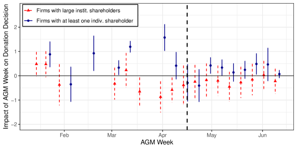
Figure 1: Shareholders’ influence on donations by AGM week

Note: The figure plots the estimated coefficients of an event study regressing whether a firm donated between January and April 2020 on dummies, indicating whether the firm held an AGM in the weeks between January 15 and June 15, 2020. The reference period is the week of June 15, 2020. Coefficients shown in circles are estimated using a sample of firms with at least one individual shareholder with at least 0.1% shares, and the triangles are from a sample of firms whose institutional blockholding (shareholders owning at least 5% a firm’s equity as of December 2019) is greater than the median at S&P 500 firms. Standard errors are clustered by industry; vertical bars denote 95% confidence intervals. The vertical dashed line is on April 15, 2020, 90 days after the first US covid case.

We note three results. First, donations are more likely at firms with individual shareholders if they hold an AGM before April 15, 2020 (dots). Second, consistent with our theory, institutional blockholders drive the decline in donation rates (triangles) as they expect dividend losses and no private returns from the donations: all else equal, the opposition to covid-donations will be more effective when institutional shareholders own more shares. Third, these two effects die out for firms that have AGMs after April 15, as shareholders at these firms have fewer incentives to influence managers: individual shareholders receive no additional image shock, which does not trigger the response of institutional shareholders.

Treatment effect. What is the effect of holding an AGM at firms with easily associable shareholders compared to the average firm? Table 2 estimates (2) by OLS, using a dependent variable that is one if firm $f$ donated by April 15 and zero otherwise as in (3) and Ownership_f defined either as the share of individual or institutional shareholders with an equity stake that, at December 2019, was either greater than 10% (Column 1 or 4), greater than 5% (Column 2 or 5), or smaller than 2% (Column 3 or 6). Ownership_f is standardized to compare coefficients across columns. Therefore, the treatment and control groups vary across columns. We standardize Ownership_f to compare coefficients across columns and estimate (2) with industry- and state-fixed effects.

Table 2: Shareholders’ influence on covid donations

	Whether Firm $f$ has Donated (0/1)
	(1)		(2)		(3)		(4)		(5)		(6)
Ownership	0.014		0.018		–0.036	∗	–0.014		–0.014		0.055	∗
	(0.017)		(0.011)		(0.020)		(0.025)		(0.026)		(0.029)
AGM	0.095		0.097		0.089		0.082		0.083		0.092
	(0.099)		(0.099)		(0.102)		(0.081)		(0.104)		(0.101)
Ownership $\times$ AGM	0.093	∗∗∗	0.096	∗∗	–0.013		–0.150	∗∗∗	–0.021		–0.033
	(0.021)		(0.034)		(0.042)		(0.043)		(0.066)		(0.065)
Ownership is defined as	Individuals						Institutional
Ownership is the share of investors owning:	$>10\%$		$>5\%$		$(0\%,2\%)$		$>10\%$		$>5\%$		$(0\%,2\%)$
Industry fixed effects	✓		✓		✓		✓		✓		✓
State fixed effects	✓		✓		✓		✓		✓		✓
$N$	433		433		433		433		433		433
Adjusted R-squared	0.1595		0.1599		0.1597		0.1668		0.1562		0.1657
* – $p<0.1$; ** – $p<0.05$; *** – $p<0.01$.

• Note: The table presents the coefficients from OLS regressions of an indicator variable that is one if firm $f$ has donated by April 15, 2020, on covariates. Italicized variables are defined in the middle panel. The variable Ownership is the share of either individual (Columns 1-3) or institutional investors (Columns 4-6) among all investors owning at least a share of total equity, as defined in the middle panel. Institutional investors include the largest financial investors in Table 1, namely, banks, mutual funds, and insurance firms. The variable Ownership is standardized. The AGM variable is an indicator variable taking value one if the firm has an AGM before April 15, 2020, and zero otherwise. All columns include industry- and state-fixed effects. Standard errors are clustered by industry.

Focusing on the interaction term, the estimated $\hat{\beta}_{treat}$ is positive and significantly different from zero for individual blockholders (Columns 1 and 2). The coefficient estimates are large as they indicate that the probability of donating increases by more than 9% compared to the average donation rate in the data when the proportion of individual blockholders increases by one standard deviation. Minority shareholders, instead, do not seem to influence company donations (Column 3). These results confirm the predictions of the conceptual framework in Section 2, which hypothesized that prominent individual investors that are more easily associated with a firm, such as those with large equity stakes, should receive a greater pass-through of image gains from the donating firm and will exert more pressure to this end.

What about institutional investors? We focus on the three largest institutional investor types in Table 1 (banks, mutual funds, and insurance firms) and find consistent results with the predictions of the conceptual framework in Section 2. The rightmost columns of Table 2 indicate that the probability of donating decreases by approximately 15% of a standard deviation of the share of large institutional blockholders (Column 4) and a negative but insignificant effect for smaller shareholding brackets (Columns 5 and 6). Thus, the largest institutional shareholders pressure managers against donations as their large equity stakes imply they will shoulder a considerable burden from the prosocial actions.

4.3 Mechanism

4.3.1 Do Equity-stakes Capture the Association between Shareholders and Firms?

Not all shareholders are created equal: some are easier to associate with a firm than others in ways not reflected in the equity stake. In this section, we proxy the degree of the association that the public holds between a firm and its most recognizable individual shareholders at the onset of the pandemic in 2020 through the maximum (Spearman) correlation between the Google Trends scores of a firm and that of its individual shareholders for the years 2018 and 2019. Hence, we define the variable $\textnormal{Ownership}_{f}$ in (2) as a dummy that is equal to one if this correlation is positive and significant at the 5% level and zero otherwise, and re-estimate (2) including state- and firm-fixed effects.

The results, displayed in Appendix Table A2, are consistent with the model laid out in Section 2, which finds that donation rates are greater for treated firms with highly-associated individual investors (Column 1). In Columns 2 and 3 we run the same analysis on subsets with increasing shares of institutional shareholders: the results suggest that the influence of recognizable individual shareholders decreases with the presence of large institutional shareholders (Columns 2 and 3). The last column indicates that large institutional shareholders are responsible for this drop in donation rates, as it finds a positive treatment effect estimate when considering only firms with many but small institutional shareholders. Therefore, only large institutional shareholders actively oppose donations.

Google search data vs. shareholding data. The Google Trend correlation measure relies on a fine-tuning parameter: starting the measurement too late in time means discounting recent events, while starting it too close to our sample period could exclude some crucial past events. In addition, we find a substantial correlation between individual blockholding and the Google Trend correlation-based measure. Finally, common ownership within an industry, a phenomenon especially present across S&P 500 corporations, might bias Internet-based measures of association between a firm and its institutional investors, as a news piece affecting the whole industry is likely to mention the largest firms within an industry, which could also be shareholders in each others’ equities. For these reasons, we focus on measures of individual and institutional shareholding in the remainder of the paper.

4.3.2 The Pass-Through of Image Gains

Our conceptual framework explains shareholder influence through a different pass-through channel of image gains across investor types. Does the data support this hypothesis? To provide direct evidence of a shock to shareholders’ private returns, we examine shareholders’ media exposure around donation events. We use shareholder names as keywords and run the following OLS regression:

$$y_{ift}=\sum_{k=-10}^{10}\psi_{k}\,\textnormal{News Day}_{it+k}+\gamma_{k}\,\textnormal{News Day}_{it+k}\times\textnormal{Individual}_{i}+\alpha_{i}+\alpha_{f}+\tau_{t}+\varepsilon_{ift},$$ (4)

where the dependent variable is the logarithm of the cumulative Google Trends score over a ten-day period starting on day $t$ for investor $i$ in firm $f$. On the right-hand side, the vector $\{\textnormal{News Day}_{it+k}\}_{k=-10}^{k=+10}$ is a set of time dummies around the date of the donation event. We further interact these indicators with another indicator variable that is equal to one if shareholder $i$ is an individual investor and zero otherwise. We also include firm, shareholder, and time-fixed effects. We interpret the coefficient vector $\psi$ as the impact of donations on Google searches for nonindividual investors and $\gamma$ as the gap in visibility between individual and nonindividual investors at each day $t+k$.

Figure 2 reports the estimated $\hat{\gamma}$, using cumulative Google Trend scores over ten days as the dependent variable and clustering the standard errors at the firm-by-shareholder level. Panel (a) uses only shareholders with at least 1% of shares in December 2019. Panel (b) restricts the sample to shareholders with more than 5% of shares. Across both panels, cumulative Google searches are flat at around zero before the donation news is broken. In Panel (a), after the news is broken, the coefficient estimates jump to about 50% from day 3 to day 10. As we might expect, the effect is stronger in Panel (b), where the coefficient estimates are already significant two days before the news is broken. Therefore, the Google search gains of individual investors are substantially higher than those of nonindividual investors, supporting our claim that image concerns create different incentives for individual and non-individual investors.

Figure 2: The gap in Google Trends of individual and institutional shareholders

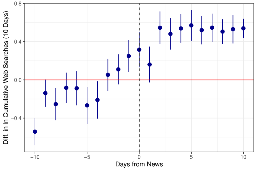
(a) Shareholders with $+1\%$ shares

(b) Shareholders with $+5\%$ shares

Note: Both panels report coefficient estimates from Equation 4, which reports the (log) cumulative Google Trends score (ten-day window) of shareholders’ names over dummy variables describing a ten window around a firms’ donation dates and the interaction of these dummies with an indicator function that is equal to one if the concerned shareholder is an individual or family shareholder and zero otherwise. The panels only report these interaction terms. Panel a (Panel b) includes only shareholders with more than 1% (5%) shares. The vertical bars indicate 95% confidence intervals using clustered standard errors by firms and shareholder types (bank, company, individual, financial company, government, hedge fund, insurance, mutual fund, self-ownership).

4.3.3 Donate Directly or Through the Financial Footprint?

Do financial investors openly oppose covid-related donations? To address this question and to understand the tradeoff faced by institutional investors, we compare the donation decisions of financial corporations in the S&P 500 (e.g., BlackRock and Bank of America) with those of the S&P 500 firms in their investment portfolios. More specifically, we analyze the correlation between two vectors: a vector of donation decisions and a vector of donation shares. The vector of donation decisions is a list of binary dummies, one for each of the 37 financial corporations in our data, indicating whether a corporation donated by April 15, 2020 (19 of them donated). The second vector reports the share of firms in the portfolio of a financial shareholder that also donated. A positive correlation between these two variables suggests an alignment in donation intents between investors and firms, while a negative correlation points to a misalignment. We exploit variation in the AGM treatment statuses of the firms in an investor’s portfolio to causally infer whether a donating investor pushes or refrains the firms in their portfolio from donating.

Table 3: Correlation of donations of financial shareholders’ and their portfolios

	Spearman Correlations
Minimum	Simple	Weighted	Weighted Avg.
Equity Share	Average	Average	$\times$ AGM
Considered	[p-values]	[p-values]	[p-values]
(1)	(2)	(3)	(4)
0%	0.442	-0.062	-0.211
(Avg. $N$ = 222)	[0.007]	[0.721]	[0.238]
1%	0.064	0.079	-0.093
(Avg. $N$ = 100)	[0.751]	[0.696]	[0.705]
2%	-0.230	0.077	-0.439
(Avg. $N$ = 57)	[0.280]	[0.721]	[0.089]
3%	-0.105	0.180	-0.617
(Avg. $N$ = 48)	[0.643]	[0.423]	[0.077]
4%	-0.112	0.060	-0.878
(Avg. $N$ = 42)	[0.630]	[0.795]	[0.021]
5%	0.124	0.275	-0.289
(Avg. $N$ = 35)	[0.637]	[0.285]	[0.638]

• Note: This table shows a negative correlation between large institutional investors such as financial firms in the S&P 500 Index and the firms in their portfolio that had their AGMs before April 15, 2020. The negative correlation indicates that financial investors opposed COVID-19-related donations in their footprints. The table computes the Spearman correlation between whether a financial firm donates and the share of donations at the firms in its portfolio. In each row, we vary the minimum share % that a firm must have in another firm to be considered an investment according to the percentages reported in the first column. Column 1 also reports the average number of S&P500 firms in the portfolio of a financial investor in parenthesis. Column 2 computes the total donations of the firms that financial firm $i$ has invested in using simple averages (i.e., $N^{-1}\times\sum_{j}\mathbb{I}_{[\text{firm }j\text{ donated}]}\times\mathbb{I}_{[i\text{'s share in }j\text{ is greater than }x\%]}$, where $N$ is the number of investments of firm $i$), Column 3 computes weighted average with weights equal to the equity shares (i.e., $\sum_{j}share_{ij}\times\mathbb{I}_{[\text{firm }j\text{ donated}]}\times\mathbb{I}_{[i\text{'s share in }j\text{ is greater than }x\%]}$), and column 4 considers only investments that got an AGM in the period under consideration (i.e., $\sum_{j}share_{ij}\times\mathbb{I}_{[\text{firm }j\text{ donated}]}\times\mathbb{I}_{[i\text{'s share in }j\text{ is greater than }x\%]}\times\mathbb{I}_{[j\text{ has an AGM}]}$). p-values testing whether the Spearman correlation is equal to zero are reported in square brackets.

Focusing first on Column 3 of Table 3, we find that the correlation coefficient between a firm’s corporate giving and the giving within its footprint is positive and even increases across rows, as we raise the minimum shareholding threshold from 0% to 5%. However, no coefficient is statistically significant. This trend may be driven by a few donating firms with larger shares receiving larger weights. Column 2 removes this effect by focusing on simple averages: the correlations are smaller and negative when the minimum shareholding threshold is 2%, 3%, or 4%. Moving to the last column, where we consider only firms with an AGM meeting, we effectively focus on firms whose shareholders might be under the spotlight due to the AGM periods and for which institutional investors might need to pressure managers to prevent individual investors from capturing private rents. As the minimum share threshold increases across rows, the estimated correlation coefficient becomes more negative and statistically significant, approaching $-1$ for larger thresholds.

These results suggest that, as we tilt the balance of influence from individual to institutional shareholders, the latter shareholders do not necessarily oppose all donations, as they donate themselves. They oppose donations at treated firms in their footprint as they do not yield any image gain but (potentially) cost them lower earnings, as we will see in Section 5.

4.4 Alternative Mechanisms

Intensity of the pandemic. Firms could respond to the need for the donation rather than shareholder pressures. Our empirical approach could miss it if, although unlikely, it is correlated with the AGM treatment. To account for this, we exploit covid cumulative cases and deaths at a firm’s headquarters state under the assumption that the severity of the pandemic will provide shareholders with greater incentives to donate even without the AGM treatment. To this end, we modify (2) as follows:

$$y_{ft} =\beta_{1}\,\textnormal{Covid Rate}_{ft}+\beta_{2}\,\textnormal{Covid Rate}_{ft}\times\textnormal{Ownership}_{f}+\beta_{3}\,\textnormal{Covid Rate}_{ft}\times\textnormal{AGM}_{f}$$ (5)

$$+\beta_{treat}\,\textnormal{Covid Rate}_{ft}\times\textnormal{Ownership}_{f}\times\textnormal{AGM}_{f}+\alpha_{f}+\tau_{t}+\varepsilon_{ft},$$

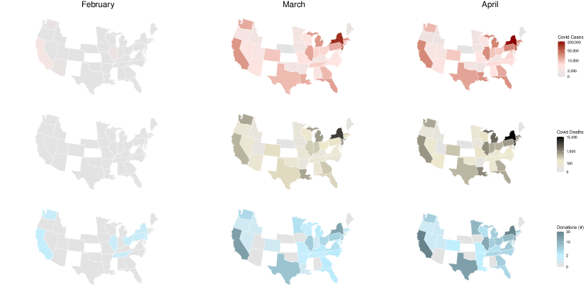
Figure B3: Covid cases, deaths, and corporate donations by US state and month

where the dependent variable, $y_{ft}$, is equal to one if firm $f$ has publicly committed to donating by day $t$ and zero otherwise. The main coefficient of interest is $\beta_{treat}$, which captures the interaction between the cumulative covid rate at firm $f$’s headquarters state, $\textnormal{Covid Rate}_{ft}$, the fraction of equity owned by the reference blockholder, $\textnormal{Ownership}_{f}$, which varies across specifications, and the AGM treatment, $\textnormal{AGM}_{f}$. We use headquarter-state covid rates because Appendix Figure B3 shows a clear spatial pattern across these two variables, with covid-related donations being more likely as the pandemic heightens. Finally, $\alpha_{f}$ and $\tau_{t}$ are firm- and day-fixed effects, and the standard errors are clustered at the firm level.

The first three columns of Appendix Table LABEL:tab:reg-results-large-shareholders present the results when individual shareholders are the reference category, with $\textnormal{Ownership}_{f}$ and $\textnormal{Covid Rate}_{ft}$ standardized to facilitate comparisons across columns with different $x$-blockholding percentages, covid cases (Panel a) and deaths (Panel b). Although the table indicates that one standard deviation in covid rates increases donation rates by about 1%-2%, such an increase is towered by the AGM treatment effect at firms with greater shares of large individual shareholders, $\beta_{treat}$, which is estimated between 10 and 20 times larger. In contrast, the treatment effect estimates when the focal blockholder in (2) varies across banks, mutual funds, and insurers are negative (Columns 4 to 12) , consistent with the previous results, and the unconditional effect of covid rates is again negligible.

Financial motives. Abnormal returns do not explain covid-related donations. To compute abnormal returns, we predict daily stock returns using the Fama-French three factors, namely, daily market returns ($R_{ft}^{MKT}$, proxied by the S&P 500 Index), daily returns on a portfolio of “small minus big stocks” ($R_{ft}^{SMB}$, from Kenneth French’s website), and daily returns on a portfolio of stocks with “high minus low” book-to-market value ratios ($R_{ft}^{HML}$, also from French’s website). We retrieve the betas ($\beta_{f}$) of those three portfolios for the stocks in our sample from CRSP. Then, stock $f$’s abnormal return ($AR_{ft}$) on day $t$ is given by the difference between the actual excess return of the stock over the risk-free rate ($R_{ft}$) and the prediction of the 3-factor model, as $AR_{ft}=R_{ft}-(\beta^{MKT}_{f}\cdot R^{MKT}_{ft}+\beta^{SMB}_{f}\cdot R^{SMB}_{ft}+\beta^{HML}_{f}\cdot R^{HML}_{ft}).$ We then plug the realized $AR_{ft}$ in the following event study:

$$y_{ft}=\sum_{-5\leq k\leq 5}\theta_{k}\,\,\text{News Day}_{ft+k}+\alpha_{f}+\tau_{t}+\varepsilon_{ft},$$

where the left-hand side refers to either firm $f$’s abnormal return ($AR_{ft}$) or its cumulative abnormal return (CAR) on day $t$. The regression includes firm- and date-fixed effects. Appendix Figure B5 displays the estimates of $\hat{\theta}_{k}$. Panel (a) shows no abnormal returns before the news is broken, while the abnormal returns are actually negative (although not significant) right after it. Panel (b) reports the CAR over five days, showing a negative drop after the news date. In summary, we find a negative but transient effect of the news on firms’ financial returns.

Consumer pressure. We exploit exogenous variation in a firm’s exposure to covid through its branches to assess whether consumers pressured firms to donate. Using the Orbis database, we compute the weighted cumulative averages of covid cases and deaths using the number of branches a firm has in each state as weights. We denote the standardized versions of these two new variables by $\textnormal{Exposure at Branches}_{ft}$ and estimate the following linear probability model:

$$y_{ft} =\beta_{1}\,\textnormal{Exposure at Branches}_{ft}+\beta_{treat}\,\textnormal{Exposure at Branches}_{ft}$$ (6)

$$\times\textnormal{Number of Branches}_{f}+\alpha_{f}+\tau_{t}+\varepsilon_{ft},$$

where $\textnormal{Number of Branches}_{f}$ is the reported number of branches as of December 2019. The results show a null effect of covid exposure (Appendix Table A3).

Managerial freedom and competition. We proxy managerial freedom with the share of a firm’s equity owned by the firm itself and study the probability of observing a donation by time $t$ using (5), where we set $\textnormal{Ownership}_{f}$ equal to one if firm $f$ owns more than the median amount of its own shares, and zero otherwise. Since the AGM period provides an opportunity for managers to present their achievements, we use the difference between the treated and control firms to estimate the causal impact of managerial’s private or image returns on donations. Although the salience of a donation in a period of crisis can help managers of underperforming firms (Akey et al., 2021; Bordalo et al., 2022b), the results indicate that managers aligned with financial investors in opposing donations potentially because if the donations are costly, as we will see in Section 5, managers might see their compensation decrease (Appendix Table A5).

We also study whether firms donated in response to past covid-related donations of a firm’s direct competitors by also controlling in (5) for a variable that is one if at least one S&P 500 firm in the industry of the focal firm has donated in the previous week and zero otherwise. Our results, presented in Appendix Table A6, show a limited role of competition while the treatment effect coefficients are very similar to those from Table LABEL:tab:reg-results-large-shareholders. Overall, these findings are in line with other studies suggesting that managers are under pressure to report positive corporate results during AGM periods (Dimitrov and Jain, 2011): large donations can jeopardize a firm’s financial position during a time of distress, potentially also affecting managerial compensation.

Missing observations in Orbis. This section has focused on a sample of firms without missing financial and ownership information in Orbis to ensure consistency across the empirical exercises. We replicate our main results – the evidence of influence by individual and institutional shareholders (Figure 1 and Table 2) and by financial shareholders within their portfolio (Table 3) – in Appendix Section D using Refinitiv’s consolidated ownership data, a slightly larger dataset, that provides historical shareholding information but, unlike Orbis, lacks self-ownership data. Across analyses, not only the signs but also the magnitude of the coefficients stays almost unchanged.

4.5 Shareholder Influence Beyond the Pandemic

Does shareholders’ influence through voice extend beyond pandemic periods? We test external validity over time and crises by focusing on another time of crisis, the recent Russian invasion of Ukraine in Section 4.5.1 and by using various measures of prosociality over the last decade in Section 4.5.2.

4.5.1 Shareholder Influence and the Russian Invasion of Ukraine in 2022

On February 24, 2022, the President of the Russian Federation, Vladimir Putin, launched the so-called “special military operation,” which started with the invasion of Ukraine and quickly escalated to a war that is still ongoing at the time of writing. Soon after that, media scrutiny of multinational corporations intensified as the public questioned the Western firms that continued to conduct business in the attacking country, Russia. As a result, many firms decided to limit their exposure to Russian consumers and businesses, with several exiting Russia altogether. In this section, we study whether a differential pass-through of image gains to individual and institutional shareholders was a factor in these decisions without discussing whether exiting was or was not the socially optimal decision. That is, we view rushed exits as consequential, costly decisions with a significant media impact that could boost the image of synonymous shareholders while costing the others substantially as firms need to pay relocation costs (e.g., suddenly seeking new suppliers and consumers than for planned exits).

Using the same approach outlined in Section 4.1, we test shareholders’ influence on exiting decisions. Once again, we take advantage of the SEC rules and exploit the occurrence of AGMs as exogenous shocks to firms’ scrutiny. To this end, we use a novel dataset that records the actions taken by international corporations vis-à-vis Russia (Sonnenfeld et al., 2022). Through this dataset, we observe the set of US-listed firms that publicly announced actions by March 23, 2022 – a month from the beginning of the conflict (164 firms). These decisions vary from exiting the country to limiting current and future investments or continuing business as usual. In particular, 51 of the 164 firms in the dataset decided to leave the Russian market. We study this radical decision because of its visibility and salience to the public. Moreover, exiting Russia goes beyond the intention of international sanctions in the first month of conflict, and thus, it was not forced by regulations.

Using (2), we identify shareholders’ voice on whether to leave Russia by setting the dependent variable, $y_{f}$, to one if firm $f$ announced its exit during the first month of conflict and zero otherwise. The regressors are instead, $\textnormal{AGM}_{f}$, which is equal to one if $f$ held an AGM in the three-month period starting on February 24, 2022, and zero otherwise, and $\textnormal{Ownership}_{f}$ which is equal to one if firm $f$ has either a shareholder of the reference type, either an individual or an institutional shareholder depending on the specification, owning more than the median share of the reference shareholder in the data. We set shareholding data at January 2022 to avoid contamination from shareholder sales. We also include several control variables such as industry fixed effects, broker recommendations, information about geographic sources of revenues, and financial standing at the end of 2021. We provide more information on the covariates and show balance tests in Appendix E.

Table 4 reports the results: Columns 1 to 3 refer to individual blockholders, while Columns 4 to 6 refer to institutional blockholders. As in the previous tables, we vary the blockholding thresholds as described in the middle panel: the magnitude of the treatment effect, $\hat{\beta}_{treat}$, increases for higher thresholds. Consistent with previous results, the presence of prominent individual shareholders positively correlates with exits, while the presence of similarly large institutional investors pushes firms’ decisions in the opposite direction.

Table 4: Shareholders’ influence on the decision to exit the Russian market

	Exited Russia in the Frist Month of Conflict (0/1)
	(1)		(2)		(3)		(4)		(5)		(6)
AGM	–0.067		–0.080		–0.094		0.144		0.035		0.043
	(0.090)		(0.087)		(0.090)		(0.115)		(0.116)		(0.111)
Above Median Blockholding	–0.547	∗∗∗	–0.542	∗∗∗	–0.428	∗∗∗	0.116		0.070		0.148
	(0.181)		(0.145)		(0.128)		(0.132)		(0.134)		(0.137)
AGM $\times$ Above Median Blockholding	0.705	∗∗∗	0.316		0.263		–0.341	∗∗	–0.152		–0.188
	(0.254)		(0.244)		(0.175)		(0.165)		(0.160)		(0.159)
Above Median Blockholding (0/1) defined for:	Individual						Institutional
Threshold to be considered a blockholder:	$>$10%		$>$5%		$>$2%		$>$10%		$>$5%		$>$2%
Controls	✓		✓		✓		✓		✓		✓
Sector fixed effects	✓		✓		✓		✓		✓		✓
$N$	138		138		138		138		138		138
Adjusted R-squared	0.2762		0.2923		0.2879		0.2642		0.2320		0.2372
* – $p<0.1$; ** – $p<0.05$; *** – $p<0.01$.

• Note: The table presents the coefficients from OLS regressions of an indicator that is one if firm $f$ has exited Russia by March 23, 2022, and zero otherwise on covariates. The regressions only exploit cross-section variation across firms at March 23, 2022. Italicized variables are defined in the middle panel. Above Median Blockholding is one if firm $f$ has more blockholders of the reference category than the median S&P 500 firm and zero otherwise. The reference category and the blockholding thresholds are defined in the middle panel. Control variables include the share of revenues that come from activities in the US and Canada, the exposure to Russia, brokers’ recommendations, CEO age, and net income. Market capitalization, revenues, and net income are highly correlated; controlling for any of these two variables instead of net income does not change the results qualitatively. For models where individual investors are the reference category (Columns 1 to 3), we also include a dummy equal to 1 for above-median institutional ownership. This variable is necessary to control whether institutional investors are heavily invested in a firm, as this channel could reduce the voice of individual and family shareholders. This variable would have been unnecessary if we could have exploited firm-fixed effects. All columns include sector-fixed effects. Robust standard errors in parenthesis.

Robustness checks. In Online Appendix E.2, we perform several tests of these empirical findings. First, we show that the negative $\beta_{treat}$ coefficient for institutional investors is mainly driven by mutual funds and banks and only partially depends on the influence of insurance company shareholders – a finding that is consistent with those in Table LABEL:tab:reg-results-large-shareholders. The results also remain unchanged by modifying equation 2 to show simultaneous treatment effects by individual and institutional blockholders through the AGM treatment or whether firms that decide for business as usual are included in the analysis. In addition, we obtain similar results when we include all US S&P 500 firms while assuming that the S&P 500 firms not surveyed by Sonnenfeld et al. (2022) took no action against Russia. Finally,exit decisions are not merely determined by the size of the firm, as measured by market capitalization or net income in 2021, indicating scope for shareholder influence.

Impacts on supply chains. Online Appendix E.3 examines supply chains. Drawing from Factset, which provides information on supply relationships between US and Russian firms, we let the dependent variable in (2), $y_{f}$, be one if firm $f$ reduced ties with Russia after February 24 and zero otherwise. Despite the size of the dataset, which covers only 102 firms with supply chains in Russia before February 24, 2022, we find that large individual shareholders indeed demanded to cut Russian suppliers.

4.5.2 Shareholder Influence Beyond Crises

Is shareholder influence on prosocial matters only limited to crisis events? We examine this question by studying firms’ ESG-related news coverage and donations during AGM periods across firms with different shares of individual shareholders. We expect the change in these variables to be only temporary because shareholders’ reputation gains should be limited to the AGM period if they drive influence.

Data. ESG-related news data come from RepRisk for 2011-2021. RepRisk screens over 80,000 media, regulatory, and commercial documents daily in fifteen different languages for adverse ESG issues called “incidents.” We focus on incidents because favorable news may come from greenwashing. Charitable donation data comes from Ravenpack, which similarly gathers news about millions of entities worldwide and identifies news about donations made by US corporations between 2011 and 2021. We merge this data with historical shareholding information from Refinitiv to get the firms’ shareholder compositions over the period. Finally, we source AGM dates from ISS. The resulting ESG-incident dataset covers 642 firms over eight years. The average firm had 772 ESG incidents in this period, of which 651 pertained to the social (“S”) category. The donation dataset spans 988 firms over 11 years, 760 of which made at least one donation for a total of 4,439 donations. The firms in the resulting datasets account for over 90% of the market capitalization of the original Ravenpack and RepRisk datasets (Appendix F describes the sample selection).

Methodology. Once again, we exploit the exogeneity of the dates of AGMs to test whether the presence of individual blockholders is associated with prosociality. Exploiting the fact that shareholders have until 120 days before the date of the release of the proxy statement of the previous AGM to submit proposals for the current AGM, we distinguish two periods: a pre-period, during which formal proposals can be cast, and a post-period, during which shareholders can engage only informally with managers and board members. We also consider two groups of firms based on their level of individual and institutional blockholders. To operationalize this analysis, we need to overcome two issues: (i) AGM dates vary across firms within a year, and (ii) firms have AGMs every year – i.e., repeated treatment. To address the first concern, we modify the calendar time of each firm so that the third month before its AGM date coincides with month 0. The pre-period starts in month -4 and ends in month 0, while the post-period lasts from period 0 to 7. Thus, a year still consists of 12 months and starts seven months before the AGM date for all firms. To address the second challenge, we stack all our yearly difference-in-differences analyses over the years as proposed in Cengiz et al. (2019). We focus on the following event study regression:

$$y_{fmt}=\sum_{k=-7,\,k\neq-4}^{4}\lambda_{k}\,\mathds{1}_{\{m+k,t\}}\times\text{Treat}_{ft}+\textbf{X}_{fmt}\,\textbf{$\beta$}+\alpha_{ft}+\tau_{mt}+\varepsilon_{fmt},$$ (7)

where to avoid double counting the same news, we define $y_{fmt}$ as an indicator that takes a value of one if firm $f$ placed at least a donation (or had an S-incident) in rebased month $m$ of year $t$ and zero otherwise. $\text{Treat}_{ft}$ is an indicator that depends on firm $f$’s ownership at the beginning of the year $t$ – we define it in the next paragraph. Thus, we control for endogenous variation in stock ownership by holding this variable constant within each year. As customary in an event study, we interact this variable with $\mathds{1}_{\{m+k,t\}}$, which is one in month $m+k$ of year $t$ and zero otherwise. We also include this variable in $\textbf{X}_{fmt}$ to adequately control for AGMs’ calendar dates as, for instance, AGMs in April and December could raise different media attention. In addition, we control for lagged quarterly cash holdings (in logs) and leverage to account for financial resources, which could vary across time and firms. Since (7) stacks multiple yearly difference-in-difference estimators, the fixed effects are at the firm-by-year, month-by-year-by-state, and month-by-year-by-industry levels. Standard errors are clustered by firm.

Results. Figure 3 presents the $\hat{\lambda}_{k}$ coefficients from estimating (7) by OLS: Panel (a) studies donations and Panel (b) social incidents. Each panel reports the estimates from two regressions based on the definition of $\text{Treat}_{ft}$ in (7). The blue dots define firms with prominent individual shareholders as treated. Red triangles consider firms with prominent institutional and no individual shareholders treated.

Figure 3: Shareholders’ influence on firms’ prosociality during AGMs

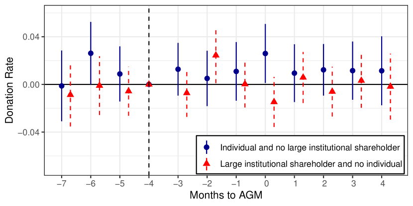
(a) Donations

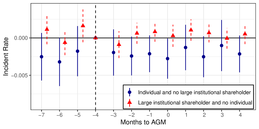
(b) Social (“S”) incidents

Note: Panel a (b) reports coefficient estimates from the event study of an indicator for whether a firm has at least a donation event (a social incident) in a given month on either a dummy that is equal to one if the firm has at least one institutional blockholder (10%) and no individual shareholder (red triangles), or a dummy equal to one if a firm has at least one individual shareholder and no institutional blockholder with at least at 10% share (blue circles). The regressions include firm-by-year, month-by-year-by-state, and month-by-year-by-industry fixed effects. Standard errors are clustered at the firm level.

We start with a null result. The red triangles never differ from zero around an AGM period. Consistent with the conceptual framework in Section 2, institutional shareholders do not exert influence against corporate prosocial behavior if they expect no shareholders to extract private gains (i.e., individual shareholders). In contrast, we observe that treated firms with individual shareholders (blue dots) are associated with prosocial actions around the AGM month ($m=0$). Panel (a) shows a statistically significant increase of 3 percentage points in donations during that month, meaning a 60% increase in the probability of observing a donation in a month. This effect is transitory and concentrated around the AGM month when media attention heightens (see Online Appendix C), and individual investors can get private returns.

The evidence is more nuanced in Panel (b). In line with our mechanism, firms with individual shareholders (blue dots) statistically have fewer social incidents only during the AGM month. However, although insignificant, the estimated coefficients are negative in all periods. To reconcile this finding, note that the social category includes not only “donations” and other readily actionable items like “violation of national legislation,” for which a prominent shareholder may exert influence in expectation of negative publicity when the firm is under the spotlight. Items like “social discrimination” and “corruption, bribery, extortion, and money laundering” are issues that might require structural changes. These items are not immediately visible to the public and might confound our results for the social category.

4.6 Summary of Results

This section empirically tested the theoretical framework outlined in Section 2 using the pandemic as the main testbed. Our main results suggest that the balance between a shareholder’s private returns and the potential earning loss due to the adoption of visible but costly prosocial decisions incentivizes shareholders to pressure managers in different directions. Exploiting AGM timings as a shock to a shareholder’s private returns, we find that individual shareholders, who are synonymous with a firm, push for greater adoption of prosocial measures (Figure 1). This result is robust to different ways of measuring the closeness of the link between a firm and its shareholders (Section 4.3.1). We support the idea of a different pass-through of image gains between individual and institutional shareholders by showing a substantial gap between Google searches of individual and institutional shareholders (Section 4.3.2). At a time of crisis, large institutional shareholders are instead those who could potentially suffer the most from costly prosocial corporate interventions if they negatively impact profits and future growth prospects of the firm they invested in. As a result, our methodology infers that these shareholders oppose donations at the footprint (Figure 1); yet, these shareholders are not necessarily against prosocial behaviors such as covid-related donations if they can reap the publicity benefits of being the donor (Section 4.3.3). In doing so, our analysis rules out several alternative channels, such as financial returns, consumer pressure, and managerial preferences (Section 4.4).

Our results are local average treatment effects because of the nature of the crisis shock. However, our findings are not limited to the pandemic: applying our framework to data from the onset of the conflict between Russia and Ukraine leads to similar conclusions (Section 4.5.1). Moreover, by exploiting firms’ ESG news coverage and donations over the last decade, we provide evidence that similar private returns incentivize individual shareholders to influence firms’ behaviors during non-crisis periods too (Section 4.5.2). Thus, our framework does not necessarily require a crisis to infer influence but only to interpret the underlying mechanism.

Finally, our framework only infers influence: we have no way to see whether actual influence took place – for instance, no shareholder proposal in 2020 considered covid-related donations – or whether managers responded to the expectation of influence from shareholders. Still, we know that managers responded to characteristics of their shareholding bodies due to the AGM treatment in a way that is consistent with shareholders’ voice over prosocial changes. How much is the cost of these positive changes for “silent” or “unheard” shareholders? We turn to this question next.

5 The Shared Costs of Influence

What are the implications for “unheard” shareholders of some shareholders’ influence on managers? Consider a simple setting where a firm has $R$ revenues and $C$ operating costs; its operating income is $\pi=R-C$. The firm can either reinvest $\pi$, which would contribute to future operating income, distribute it as a dividend to its shareholders, or surrender to shareholders’ voice and spend it in non-productive ways such as a donation (as in Section 4) or a disorganized exit from Russia (as in Section 4.5.1). If the firm opts for the non-productive choice, the discounted value of future operating incomes could drop, resulting in a net loss for all shareholders who cannot extract private benefits from it (e.g., image returns).

Measuring a firm’s productivity is generally tricky. Nevertheless, we have access to two variables that, together with the shocks provided by the exogenous timing of AGMs and external crisis, ease our identification problem: operating income and market capitalization. The first variable speaks directly about how much revenue a firm can raise for each dollar spent in costs and is often used as a row measure of productivity, given demand (e.g., Harberger, 1954; Baqaee and Farhi, 2020). The second one provides insight into the discounted loss to shareholders through changes in stock prices.

As productivity impacts both $R$ and $C$, we cannot identify productivity changes without accounting for changes in demand affecting $R$, and there are reasons to believe that consumer demand reacted both to covid and the invasion of Ukraine through lockdowns and consumer protests. However, it is safe to believe that potential demand changes are unrelated to the share of individual and institutional shareholders before the crisis (Section 4.4). Our approach employs a triple differences-in-difference estimator, which leverages this intuition. We consider a firm as treated if it held an AGM at the onset of the crisis and control otherwise. We then distinguish firms into two more groups based on whether they had large individual shareholders just before the crisis. Identification only requires that the relative change in outcomes between firms in the two groups trended similarly for treated and control firms, a milder requirement than for standard difference-in-differences model (Olden and Møen, 2022).

5.1 Data

We perform our analysis on two samples. The first sample exploits the pandemic and focuses on the 1,000 largest US-listed firms just before the pandemic hit the country (December 2019) to study their productivity between 2013 and 2022. For the Ukraine invasion case, instead, we restrict our analysis to quarterly data between 2020 to the third quarter of 2022 to capture the immediate effects of a disorganized exit from Russia. We further restrict our sample to firms that dealt with Russian counterparts before 2022, excluding those with no revenue from Russia, according to Refinitiv, because these firms are impacted only indirectly by this crisis. The final sample consists of the largest 1,153 US-listed firms with dealings with Russia. Therefore, the first sample includes much larger firms than the second one, with operating income and market capitalization four times greater on average. The Ukraine-Russia sample is also more heterogeneous, displaying operating incomes almost two times more skewed than in the covid sample. In both samples, historical ownership and financial data are from Refinitiv and Compustat, while AGM dates are from ISS.

5.2 Methodology and Results

5.2.1 Crisis 1: Covid Pandemic

Starting from the covid crisis, the left panels of Figure 4 display quarterly average operating income and market capitalization by group and treatment condition between 2016 and 2022. Treated (control) firms are displayed with solid (dotted) lines, and firms with (without) large individual shareholders are in bold blue (red). The average trends by groups look parallel, especially in the years immediately before 2020. In contrast, especially in 2020 and 2021, the gap between the bold blue and red solid lines widens while that between the two dotted lines shrinks: we infer that operating income and stock prices dropped at the firms where shareholders had the most to gain from prosocial actions, highlighting negative consequences for other shareholders.

Figure 4: Documenting rents: covid case

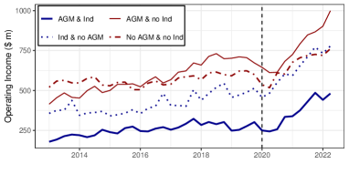
(a) Operating income (quarterly data)

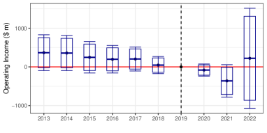
(b) Operating income - event study

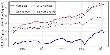
(c) Market cap (quarterly data)

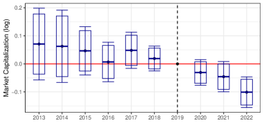
(d) Market cap (log) - event study

Note: Panels (a) and (c) plot the operating income and the market cap (in logs) for firms with and without an AGM between January 15 and April 15, 2020, and at least an individual shareholder with a 5% shares. Panels (b) and (d) plot the estimated coefficients from (8), where the coefficients of interest are the interaction between time dummies, a dummy equal to one if the firm holds an AGM between January 15 and April 15, 2020, and the share of individual shareholders with at least a 5% share. The regressions include controls and firm, year, and year-by-industry fixed effects. Standard errors are clustered at the industry and state levels. Error bars (boxes) report the 95% (90%) CI. Vertical dashed lines indicate the two events.

To assess magnitude changes, the right panels estimate the following event study:

$$y_{ft}=\sum_{k\neq 2019}\theta_{k}\;\mathds{1}_{\{t+k\}}\times\text{Treat}_{f}\times\text{Ownership}_{f}+\textbf{X}_{ft}\;\textbf{$\beta$}+\alpha_{f}+\tau_{t}+\iota_{i(f)t}+\varepsilon_{ft},$$ (8)

where the dependent variable is operating income or market capitalization (in logs). As in Panel (a), Treat_f are the firms that held an AGM in the 90 days after January 15, 2020, and Ownership_f is the share of individual shareholders with at least a 5% equity-share, which we standardize to interpret $\theta_{k}$ in terms of standard deviations in individual ownership. The direct effect of ownership and treatment status in each month $t+k$ is accounted for in $\textbf{X}_{ft}$, which also includes lagged assets to control for variation in firm size. The fixed effects are at the firm, $\alpha_{f}$, year, $\tau_{t}$, and industry-by-year, $\iota_{i(f)t}$, levels, with the latter capturing the average impact of the crisis across industries. The regression residuals are likely correlated within states (e.g., state policy) and across firms in the same industry (e.g., demand responses). Thus, we cluster the standard errors at these levels.

Panels (b) and (d) measure the effect of shareholders’ voice on productivity. Operating income dropped immediately in 2020 by $81m of a standard deviation and dropped further in 2021 by $359m (p-value: 0.09) before returning to its pre-covid values. On average, we estimate in Appendix Table A7 that a 1% increase in the share of individual investors with at least a 10% share costs the other shareholders less operating income for $130m (p-value $\leq 5\%$). A similar increase in the share of individual investors owning 5% leads to a more modest $76 m loss (p-value $\leq 5\%$). The average treatment effect can be summarised in a -1.7% in yearly operating income. In addition, we find that the loss is entirely driven by concentration among large individual shareholders (cf. Columns 1 and 3 of Appendix Table A7), further validating the mechanism exposed in Section 2.

Mechanism: fewer investments at treated firms. Operating income could drop because of greater costs, $C$, or less revenues, $R$. Appendix Figure B6 shows that sales as a fraction of total assets stayed constant at treated and control firms, while the fraction of total assets covered by operating income declined sharply after 2020, a finding that resonates well with our results in Section 4.4 indicating that consumer demand did not impact covid donations. As donations are costly, Appendix Figure B7 finds that shareholders’ voice decreased a firm’s cash holding in 2020 and 2021. Less cash led to fewer investments, especially in the manufacturing sector, where total investments dropped by between 4% and 10% (p-value $\leq 0.08$) of a standard deviation, compared to 2019 (Appendix Figure B8). As a result, shareholders at treated firms immediately felt the cost of the decline in productivity. Panel (d) of Figure 4 shows a steady decline in market capitalization by between 5% and 8% of a standard-deviation. This average loss to shareholders is substantial: Column 3 (4) of Appendix Table A7 measures it in a 4% (3%) change per 1% increase in individual shareholders with at least 10% (5%) share.

5.2.2 Crisis 2: Invasion of Ukraine

Figure 5 replicates the analysis using the Ukrainian invasion as a testbed. Panel (b) runs an event study similar to (8) on quarterly operating income. Because of skewness and negative values in quarterly operating incomes, we present results after applying an inverse hyperbolic transformation to the dependent variable. In the first quarter of 2022, the coefficient estimated for the transformed operating income dropped by about 10% of its average value before 2022 per each standard deviation of the share of individual blockholders, before recovering by Q3 2022. As for the covid crisis, we find that shareholders faced an immediate loss as the stock market of the most exposed firms to individual shareholders’ voices dropped by 6%-8% of a standard deviation in each quarter after the crisis broke. The cost to shareholders is similar to that from the covid crisis, measurable in 1% of quarterly market capitalization for a 1% increase in individual blockholding (Appendix Table A7).

Figure 5: Documenting rents: Russian invasion of Ukraine

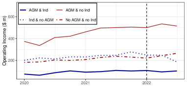
(a) Operating income

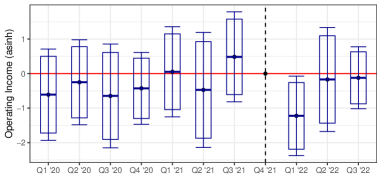
(b) Operating income - event study

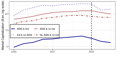
(c) Market cap

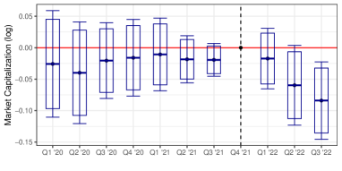
(d) Market cap (log) - event study

Note: Panels (a) and (c) plot the operating income and the market cap (in logs) for firms with and without an AGM between February 24 and May 24, 2022, and at least an individual shareholder with a 5% shares. Panels (b) and (d) plot the estimated coefficients from (8), where the coefficients of interest are the interaction between time dummies, a dummy equal to one if the firm holds an AGM between February 24 and May 24, 2022, and the share of individual shareholders with at least a 5% share. The regressions include controls, firm, time, and time-by-industry-fixed effects. Standard errors are clustered at the industry and state levels. Error bars (boxes) report the 95% (90%) CI. Vertical dashed lines indicate the two events.

Mechanism: restructuring costs. As before, we investigate changes in revenue or costs as the main source of the loss observed at treated firms. Appendix Figure B11 finds that operating income as a fraction of assets dropped substantially while sales remained constant, indicating that the costs of rushing out of Russia, such as finding new suppliers as suggested in Section 4.5.1, tower the lost Russian revenues. This interpretation is also consistent with the timing of the government sanctions that eventually imposed no dealing with Russian entities for most, if not all US firms, so we can conclude that rushed exits did not cost in terms of consumers as much as it increased costs. What are these costs? Fleeing past investments, potentially at a highly discounted price or loss, might be a credible hypothesis. Consistent with it, Panel (a) of Appendix Figure B12 finds that treated firms sold their past investments at a substantially higher rate than control firms: 20% more sales per standard deviation increase in the share of individual blockholders in each quarter after the crisis. The associated costs are visible in Panel (b), which plots the differential evolution of the cash-to-asset ratio, highlighting a drop as high as 3% per standard deviation of the share held by individual blockholders.

5.3 Discussion: “The Cost for Unheard Shareholders”

In the previous sections, we inferred that highly visible and potentially connected shareholders motivated by personal interests seek to extract rents by influencing firms to take visible but costly prosocial actions. By assessing their distributional cost across the shareholding body, this section estimates a “welfare cost” of shareholders’ voice without engaging in a formal welfare analysis that would be far-fetched without data to assess the social benefit of an extra in-kind donation. We find that shareholder influence has non-negligible distributional consequences for “silent” shareholders: our intent-to-treat framework estimates an average treatment effect of -1.7% in yearly operating income and -3.36% in market capitalization for the covid case. The drop is even starker among treated firms, which lost about 7% of yearly operating income. Despite a different mechanism, the Ukraine-Russia case finds slightly smaller but comparable drops in quarterly operating income and market capitalization.

The sudden timing of these drops in key productivity measures is consistent with the proposed mechanism. Based on quarterly data, the Ukraine-Russia case illustrates the timing effect well: the drop in operating income is in the quarter immediately after the invasion (Figure 5), and it reverberates in a steady decline in market capitalization across all quarters of 2022 at treated firms. We find that the increase in operating costs is related to relocating activities and selling past investments in a disorganized manner: Panel (b) of Figure B13 finds that restructuring charges reached $0.3 per share more at treated than at control firms after the invasion, or 5% of the average pre-crisis earnings per share (EPS), which measure the net income distributed to each outstanding share.

In contrast, the yearly data in the covid case allow us to investigate how influence dynamically impacts future shareholder outcomes. The mechanism still relies on changes in investments. However, this time, in-kind donations reduced cash flows by imposing variable operating costs (e.g., inputs and personnel) without increasing revenues. These expenses ate resources that would have been otherwise available for future investments: Panel (a) of Figure B13 shows that EPS dropped in 2020 and 2021, two years after the start of the pandemic, by about $0.4 - $0.8 more at treated firms, or over 8% of the average EPS in 2019. Thus, influence does not only cost shareholders a portion of their current potential payoffs but also future ones. We conclude that those shareholders who could not yield private benefits from the firms’ prosocial actions made overall a loss. Thus, shareholder influence, even on ESG matters as “trivial” as donating to fight COVID-19, has substantial distributional consequences.

This paper brings new data and empirical methods to normative questions regarding what firms should do in similar situations (Friedman, 1970; Baron, 2007). While some positive corporate decisions could create value for society at large – i.e., corporate donations to hospitals of items such as face masks that shareholders would have been unable to procure themselves – and thus, it might be optimal from a societal point of view that firms undertake them as discussed in a seminal paper by Hart and Zingales (2017), we find that not all shareholders value them equally. As suggested by Bartlett and Bubb (2023) and Edmans (2023), for corporations to have social responsibilities beyond the profit motive, shareholders must support corporations’ socially responsible actions; without it, managerial decisions do not represent shareholders’ values and create tensions among shareholders. Given that only major issues or disagreements make it to AGMs for voting, most shareholder disagreements are unobservable to outsiders. To determine whether shareholders support these actions, we develop a portable framework to infer shareholder preferences about corporations’ socially responsible actions. When considering large corporations with diffuse shareholders, the losers among the shareholders (e.g., households saving through financial intermediaries) can potentially be many more than the actual winners.

Extending the spectrum of our analysis, shareholder conflicts might also have welfare consequences for other stakeholders, such as workers, consumers, or the environment, effectively implementing a redistribution toward social causes (e.g., Baron, 2001). In these cases, managerial decisions could overweight or underweight the payoff to concerned stakeholders compared to the objective of an elected representative, as, for instance, managers might respond to stock prices or their stock options, matters that are of no concern for elected officials. Therefore, the mere existence of a positive or negative externality (e.g., the potential to enact private sanctions on a villain state) does not authorize managers to solve it (Edmans, 2023). More research is needed to assess the consequences of heterogeneity across shareholders’ values and influence for other shareholders and society at large, both empirically (e.g., Allcott et al., 2022; Fioretti, 2022) and normatively (e.g., Hansmann, 2000; Elhauge, 2005; Broccardo et al., 2022).

“Who watches the watchmen?” Despite uncovering unobserved tensions among shareholders, we do not believe that shareholders should vote on each possible action: this would not only be impractical, but it also defies the very reason for having a qualified management team. Nevertheless, there are several ways for managers to learn about their shareholder preferences. For instance, most companies meet with their largest shareholders regularly (Edmans, 2023). Even without meetings, some shareholders are particularly vocal about their values, as shown by Bill Ford in the introduction to this article, meaning that shareholders are aware of each other’s preferences. Our results indicate that large shareholders monitor each other and anticipate each other’s motives to influence managers. The monitoring is triggered by (i) the balance of shareholder preferences, (ii) the cost of their influence on managers, and (iii) the potential future earning losses (see Section 2). Therefore, shareholder preferences matter for a firm’s efficiency and the protection of minority rights. In past years, an extensive literature has developed investigating the pros and cons of the monitoring role over managers of a firm’s largest shareholders (e.g., Shleifer and Vishny, 1997). Our findings refocus this literature around the preferences of large shareholders: since only large shareholders might have enough to lose from mismanagements, they have incentives to monitor managers and shareholders; if all large shareholders have the same preferences, they might all seek the same rents at the cost of minority shareholders and other stakeholders (e.g., workers). Hence, heterogeneity among blockholders creates value for minority shareholders, a hypothesis that future research could test using stock market data.

Empirical contribution. We also contribute methodologically to the debate about shareholder preferences by providing a framework that links (specific) shareholder preferences to firms’ prosocial actions to infer the unobserved pressures exerted by shareholders on managers. Moreover, the proposed framework is portable across time and countries (see Sections 4.5.1 and 4.5.2). On the other hand, standard techniques studying AGM votes would not teach us much regarding shareholder preferences, as most shareholder conflicts might not emerge at AGMs – for instance, no shareholder was called to vote upon covid donations at AGMs in 2020.

This new framework opens several avenues for future research as our approach cannot tell whether managers react to the realized pressure or influence of some shareholders or whether they react to this expectation. Addressing the determinants of these managerial expectations is necessary for policies aiming at improving governance and communication between stakeholders. Behaviorally, shareholders’ preferences can be micro-founded through a warm glow utility as in Andreoni (1989) or reputation concerns as in Bar-Isaac et al. (2008). One possible way to empirically distinguish these two channels is to exploit repeated shocks to learn whether a shareholder’s influence declines over time – conditional on not selling her shares – as her reputation gains reach a plateau, which would be consistent with signaling. However, this exercise is infeasible with our data, as we take advantage of single large sudden shocks, and thus, we view these motives as externalities that shareholders inflict on other shareholders.

Thus, while our framework is suitable for establishing causality, it might not be able to assess shareholder welfare changes in different counterfactual scenarios. For example, policymakers might ask about firms’ behaviors and total welfare changes if policies reducing coordination costs between managers and shareholders (e.g., Aghion and Tirole, 1997; Landier et al., 2009; Harris and Raviv, 2010) or different managerial compensations (e.g., Baker et al., 1988; Bandiera et al., 2009; Saint-Jean, 2023) are in place. A complete model of shareholder preferences might help in this case: this requires modeling the purely altruistic preferences, which we do not discuss in this paper because they are net out by the control group, and understanding the root of shareholders’ private gains. We view these questions as fertile grounds for future research.

In conclusion, the transition toward a more sustainable economy expands the source of rents for shareholders by adding new concerns, such as private image gains, to already existing ones, like profit motives. As the quote by Grossman and Hart (1979) in the introduction states, our study suggests that today it is more important than ever that “the manager of a firm […] not only […] organize production, but also learns about the preferences of the firm’s shareholders.” We view this paper as a first step in this direction.

6 Conclusion

Stakeholders influence a firm’s strategy. This paper offers a portable framework that exploits quasi-experimental variations commonly available at all listed corporations to investigate how shareholders, a central stakeholder, impact firms’ strategies over visible but costly prosocial decisions. We apply our framework to corporate decisions to donate for covid relief during the pandemic and to exit the Russian market as a private sanction after Russia invaded Ukraine. In both settings, the prosocial decision is optimal for shareholders if they care for the issue at stake; for instance, a large chemical corporation might be in a better position to provide sanitizing gels and facemasks during the pandemic than what the donations of a shareholder to an NGO can buy. However, what is the optimal action if shareholders have different preferences?

We show that firms are more likely to adopt costly prosocial changes if their shareholding body includes easily recognizable individual and family investors. In contrast, significant financial shareholding had the opposite effect on corporate donations. We explain the different influences exerted by these shareholders in terms of a heterogeneous pass-through of image gains to a firm’s shareholders using internet search data. Thus, shareholders face different tradeoffs because they have different preferences: all shareholders bear the cost of a firm’s decision, but only some derive positive image gains. As a result, pursuing “shareholder value” might come at a cost for other shareholders. Consistent with this hypothesis, we find a significant and sustained drop in productivity after the pandemic and the Russian invasion. We exploit the different features of the two crises to investigate and interprete different channels for shareholder influence to negatively affect productivity and provide evidence that large shareholders monitor each other.

Online Appendix

Appendix A Omitted Tables

Table A1: The impact of institutional blockholders on covid donations

	Whether Firm $f$ has made a Donation (0/1)
	(1)		(2)		(3)		(4)		(5)		(6)		(7)		(8)		(9)
Ownership	–0.030		–0.018		0.100	∗∗∗	–0.026		–0.038		–0.105	∗∗∗	0.058	∗∗∗	0.069	∗∗∗	0.018
	(0.020)		(0.017)		(0.025)		(0.016)		(0.025)		(0.020)		(0.012)		(0.010)		(0.030)
AGM	0.094		0.077		0.089		0.082		0.093		0.090		0.099		0.086		0.082
	(0.090)		(0.098)		(0.098)		(0.097)		(0.102)		(0.103)		(0.098)		(0.095)		(0.111)
Ownership $\times$ AGM	–0.073	∗∗	–0.020		–0.049		–0.030		–0.002		0.083	∗∗	–0.142	∗∗∗	–0.040		–0.049
	(0.030)		(0.062)		(0.046)		(0.043)		(0.035)		(0.030)		(0.018)		(0.059)		(0.079)
Constant	0.033		0.038		0.049		0.042		0.033		–0.002		0.057		–0.004		0.069
	(0.071)		(0.064)		(0.067)		(0.075)		(0.078)		(0.035)		(0.065)		(0.017)		(0.072)
Ownership is defined as:	Banks						Mutual Funds						Insurance
Ownership is the shares of shareholders owning:	$>$10%		$>$5%		$(0\%,2\%)$		$>$10%		$>$5%		$(0\%,2\%)$		$>$10%		$>$5%		$(0\%,2\%)$
Industry fixed effects	$\checkmark$		$\checkmark$		$\checkmark$		$\checkmark$		$\checkmark$		$\checkmark$		$\checkmark$		$\checkmark$		$\checkmark$
State fixed effects	$\checkmark$		$\checkmark$		$\checkmark$		$\checkmark$		$\checkmark$		$\checkmark$		$\checkmark$		$\checkmark$		$\checkmark$
$N$	433		433		433		433		433		433		433		433		433
Adjusted R-squared	0.1638		0.1565		0.1909		0.1575		0.1606		0.1921		0.1716		0.1696		0.1559
* – $p<0.1$; ** – $p<0.05$; *** – $p<0.01$.

• Note: This table zooms in on which institutional blockholders impacted covid-related donations the most. The table presents the coefficients from OLS regressions of an indicator variable that is one if firm $f$ has donated by April 15, 2020, on covariates. Italicized variables are defined in the middle panel. The variable Ownership is the share of institutional investors (of the reference category defined in the middle panel) among all investors owning at least a share of total equity as defined in the middle panel. The variable Ownership is standardized. The AGM variable is an indicator variable taking value one if the firm has an AGM before April 15, 2020, and zero otherwise. All columns include industry- and state-fixed effects. Standard errors are clustered by industry.

Table A2: The influence of individual shareholders associated with a firm using Google Trend data

	Whether Firm $f$ has donated (0/1)
	(1)		(2)		(3)		(4)
Association	-0.061		-0.096		-0.076		-0.124
	(0.073)		(0.070)		(0.163)		(0.80)
AGM	0.014		0.036		-0.170		-0.160
	(0.081)		(0.088)		(0.236)		(0.089)
Association $\times$ AGM ($\beta_{treat}$)	0.298	∗∗	0.342	∗∗	-0.878	∗	0.704	∗∗
	(0.128)		(0.136)		(0.455)		(0.222)
Difference $\beta_{treat}$ with Column (1)	-		-0.044		1.176	∗∗	-0.406
(p-value)	(-)		(0.799)		(0.015)		(0.118)
Subset	At least one institutional						Above
	shareholder with						median
	$\geq$ 0%		$>$5%		$>$10%		inst. shar.
State fixed effects	✓		✓		✓		✓
Industry fixed effects	✓		✓		✓		✓
N	457		395		89		223
Adjusted R-squared	0.2458		0.2519		0.5405		0.3406
* – $p<0.1$; ** – $p<0.05$; *** – $p<0.01$.

• Note: This table studies whether the influence of individual shareholders highly associated with a firm increases during an AGM period and whether institutional blockholders act to sabotage individual shareholders’ influence. The table presents OLS regressions of whether firm $i$ has donated by April 15, 2020, on covariates. Association_f is an indicator variable equal to one if a firm has at least one individual shareholder with whom its Google Trends score is positively and significantly correlated with the firm’s Google Trends score. This association is measured by the Spearman correlation statistic using data for 2018 and 2019. AGM_f is an indicator variable equal to one if the firm has an AGM in the sample period and zero otherwise. We vary the estimation subset across columns to include all observations (Column 1), only firms with institutional blockholders with at least 5% (Column 2), or 10% (Column 3) equity shares. The last column studies whether the effects are due to institutional shareholding instead of institutional blockholding by including only firms with more than 47% shares owned by institutions (i.e., disregarding the specific ownership of each shareholder). Overall, the results indicate that institutional blockholders, rather than shareholders act to reduce individual shareholders’ influence, which is consistent with the conceptual framework in Section 2. The middle panel displays the difference between the interaction coefficient $\beta_{treat}$ in Columns 2 to 4 with that in Column 1. All columns include industry- and state-fixed effects. Standard errors are clustered by industry.

Table A3: The impact of covid exposure at branches on donations

	Whether Firm $f$ has Donated by Time $t$ (0/1)
	(1)		(2)		(3)		(4)		(5)		(6)		(7)		(8)
Exposure at branches	0.007		0.009		0.012		0.014		0.008		0.008		0.010		0.011
	(0.017)		(0.013)		(0.012)		(0.012)		(0.015)		(0.011)		(0.010)		(0.010)
Exposure at branches $\times$ Number of branches ($\ln$)	0.003								0.001
	(0.005)								(0.005)
Exposure at branches $\times$ More than $x$ branches			0.024		0.039		0.020				0.018		0.039		0.016
			(0.024)		(0.028)		(0.045)				(0.024)		(0.029)		(0.050)
Exposure at branches is defined as:	Cumulative cases								Cumulative deaths
More than $x$ branches (0/1) is 1 if the firm has
more branches than the $x$ quantile:			50%		75%		90%				50%		75%		90%
Time fixed effects	$\checkmark$		$\checkmark$		$\checkmark$		$\checkmark$		$\checkmark$		$\checkmark$		$\checkmark$		$\checkmark$
Firm fixed effects	$\checkmark$		$\checkmark$		$\checkmark$		$\checkmark$		$\checkmark$		$\checkmark$		$\checkmark$		$\checkmark$
$N$	33,490		37,570		37,570		37,570		33,490		37,570		37,570		37,570
Adjusted R-squared	0.4979		0.4967		0.4969		0.4958		0.4978		0.4961		0.4965		0.4956
* – $p<0.1$; ** – $p<0.05$; *** – $p<0.01$.

• Note: This table finds that consumers were not a driver of covid-related donations because covid exposure in the states where firms had their branches does not correlat with donations rates across firms. The table presents the coefficients from OLS regressions based on Equation 6 based on an indicator variable that is one if firm $f$ has donated by day $t$ and zero otherwise on covariates. Italicized variables are defined in the middle panel. Columns 1 to 4 use cumulative covid cases at the headquarters state, and Columns 5 to 8 use cumulative covid deaths. The variable Number of branches in Columns 1 and 5 is in log. The remaining columns use a dummy variable (More than $x$ branches) for whether the focal firm has more than the $x$-percentile than the distribution of brunches: this value is 40 branches in Columns 2 and 6, 170 branches in Columns 3 and 7, and 664 branches in Columns 4 and 8. Orbis data do not report branches for 15 firms, which are therefore omitted from the analysis. All columns include day- and firm-fixed effects. For this reason, the table does not report the direct effect of the Number of Branches, which does not vary over time and, thus, is captured by the firm-fixed effects. The dataset starts on January 15, 2020 and ends on April 15, 2020. Standard errors are clustered by firm and presented in parenthesis.

Table A4: Abnormal and cumulative abnormal returns, using stock return forecasts based on data from the 60 days before a donation announcement

	Abnormal		Comulative Abnormal Returns
	Returns		7 days		10 days		14 days
	(1)		(2)		(3)		(4)
10 Days Before	–0.136		0.543		0.216		–0.771
	(0.302)		(0.789)		(0.806)		(0.768)
9 Days Before	–0.172		1.197		0.106		–0.734
	(0.365)		(0.889)		(0.868)		(0.837)
8 Days Before	0.168		1.219		0.879		–0.255
	(0.333)		(0.997)		(0.946)		(0.892)
7 Days Before	0.524		0.267		0.228		–0.568
	(0.352)		(1.078)		(0.982)		(0.981)
6 Days Before	–0.204		–0.208		–1.166		–1.555
	(0.478)		(1.070)		(1.010)		(1.070)
5 Days Before	–0.418		0.747		–0.944		–1.242
	(0.432)		(0.977)		(0.970)		(1.017)
4 Days Before	0.961	∗∗	0.786		–0.436		–1.138
	(0.407)		(0.951)		(0.972)		(1.036)
3 Days Before	0.761		–1.396		–1.149		–2.140	∗
	(0.464)		(1.051)		(1.045)		(1.129)
2 Days Before	–0.426		–2.204	∗∗	–2.674	∗∗	–3.544	∗∗∗
	(0.539)		(1.116)		(1.100)		(1.239)
1 Day Before	–0.702		–1.571		–2.381	∗∗	–3.226	∗∗
	(0.559)		(1.202)		(1.140)		(1.343)
Day of the Donation	–0.334		–1.054		–1.944	∗	–2.777	∗
	(0.544)		(1.286)		(1.110)		(1.485)
1 Day After	0.929		–1.453		–1.866	∗	–2.536	∗
	(0.598)		(1.113)		(1.042)		(1.414)
2 Days After	–1.036	∗	–2.201	∗∗	–3.404	∗∗∗	–3.799	∗∗∗
	(0.540)		(1.077)		(1.102)		(1.403)
3 Days After	–1.337	∗∗	–1.043		–2.046	∗	–2.444
	(0.547)		(1.055)		(1.117)		(1.488)
4 Days After	0.827		0.144		–0.108		–0.346
	(0.523)		(1.293)		(1.280)		(1.630)
5 Days After	0.046		–1.144		–1.132		–1.588
	(0.769)		(1.507)		(1.420)		(1.867)
6 Days After	0.606		0.171		–1.353		–1.470
	(0.755)		(1.345)		(1.418)		(1.670)
7 Days After	–0.717		–0.288		–1.733		–1.240
	(0.555)		(1.046)		(1.250)		(1.338)
8 Days After	–0.366		0.940		0.106		0.312
	(0.641)		(1.110)		(1.411)		(1.274)
9 Days After	0.063		0.790		1.578		1.540
	(0.525)		(0.979)		(1.134)		(1.112)
10 Days After	1.214		0.969		1.689		1.985
	(0.764)		(1.403)		(1.331)		(1.456)
Time fixed effects	$\checkmark$		$\checkmark$		$\checkmark$		$\checkmark$
Firm fixed effects	$\checkmark$		$\checkmark$		$\checkmark$		$\checkmark$
$N$	22,246		22,246		22,246		22,246
Adjusted R-squared	0.0331		0.1039		0.1401		0.1880
* – $p<0.1$; ** – $p<0.05$; *** – $p<0.01$.

• Note: This table reports the coefficients from an event study using the abnormal returns (ARs) and cumulative abnormal returns (CARs) around the day of the donation (model 4.4). ARs are computed as the difference between realized excess returns and the prediction of a one-factor model (the market factor), for which the stock’s beta is computed over the last 60 days. The sample period goes from January 1 to April 15, 2020. All columns include firm and day-fixed effects. Standard errors are clustered by firm and are presented in parenthesis.

Table A5: The impact of self-ownership on covid donations

	Whether Firm $f$ has Donated by Time $t$ (0/1)
	(1)		(2)		(3)		(4)		(5)		(6)
Covid Rate	0.022	∗∗	0.019	∗∗	0.114	∗∗∗	0.100	∗∗∗	–0.003		–0.001
	(0.011)		(0.009)		(0.007)		(0.006)		(0.015)		(0.012)
Covid Rate $\times$ Ownership	–0.035		–0.034		–0.019		–0.016		0.010		–0.007
	(0.028)		(0.024)		(0.028)		(0.026)		(0.060)		(0.052)
Covid Rate $\times$ AGM	0.067	∗	0.057	∗∗∗	0.028		0.025		0.068		0.084
	(0.038)		(0.021)		(0.028)		(0.025)		(0.055)		(0.070)
Covid Rate $\times$ Ownership $\times$ AGM	–0.109	∗∗	–0.091	∗∗∗	–0.079		–0.075		–0.024		0.075
	(0.048)		(0.031)		(0.068)		(0.063)		(0.283)		(0.349)
Covid Rate is defined as:	Cases		Deaths		Cases		Deaths		Cases		Deaths
Ownership (0/1) is:	High self-ownership				High self-ownership				High self-ownership
	At Headquarter				National Rates				At Branches
Time fixed effects	$\checkmark$		$\checkmark$		$\checkmark$		$\checkmark$		$\checkmark$		$\checkmark$
Firm fixed effects	$\checkmark$		$\checkmark$		$\checkmark$		$\checkmark$		$\checkmark$		$\checkmark$
$N$	38,845		38,845		38,845		38,845		29,665		29,665
Adjusted R-squared	0.4958		0.4948		0.4927		0.4924		0.5007		0.5006
* – $p<0.1$; ** – $p<0.05$; *** – $p<0.01$.

• Note: This table finds that greater self-ownership shares negatively affect the probability that a firm donates. We use this variable as a proxy for managerial freedom. Thus, the table implies that managers did not favor donations. The table presents the coefficients from OLS regressions based on Equation 5 of an indicator variable that is one if firm $f$ has donated by day $t$ and zero otherwise on covariates. Italicized variables are defined in the middle panel. We vary the definition of Covid Rate across columns. Columns 1 and 2 measure covid at the headquarters state, Columns 3 and 4 measure covid at the national level, and Columns 5 and 6 measure covid at the state of the branches using the number of branches as weights. The last two columns restrict the data to firms with at least five branches. The variable Ownership is one if the share of equity owned by the firm itself is greater than its median value in the dataset and zero otherwise. The variable Covid Rate is standardized. The AGM variable is an indicator variable taking value one if the firm has an AGM before April 15, 2020, and zero otherwise. All columns include day- and firm-fixed effects. The interaction Ownership $\times$ AGM and the direct effect of the variables Ownership and AGM are accounted for by the firm-fixed effects. The dataset starts on January 15, 2020, and ends on April 15, 2020. Standard errors are clustered by firm and presented in parenthesis.

Table A6: The impact of individuals blockholders on covid donations

	Whether Firm $f$ has Donated by Time $t$ (0/1)
	(1)		(2)		(3)		(4)		(5)		(6)		(7)		(8)
Competitor Donating (0/1)	0.018	∗	0.017	∗	0.018	∗∗	0.017	∗	0.018	∗	0.018	∗	0.018	∗∗	0.018	∗
	(0.009)		(0.009)		(0.009)		(0.009)		(0.009)		(0.009)		(0.009)		(0.009)
Cum. Covid Rate	0.021		0.023	∗	0.050	∗∗	0.023	∗	0.018		0.020	∗	0.042	∗∗	0.020	∗
	(0.013)		(0.013)		(0.024)		(0.013)		(0.012)		(0.011)		(0.021)		(0.012)
AGM $\times$ Cum. Covid Rate	0.047		0.023		0.145	∗∗	0.008		0.062		0.023		0.159	∗∗∗	-0.019
	(0.053)		(0.052)		(0.068)		(0.052)		(0.054)		(0.048)		(0.049)		(0.036)
Ownership $\times$ Cum. Covid Rate	0.008	∗∗	-0.020	∗∗	-0.056		-0.003		0.007	∗	-0.017	∗∗	-0.046		-0.003
	(0.004)		(0.009)		(0.043)		(0.009)		(0.004)		(0.008)		(0.040)		(0.008)
AGM $\times$ Ownership $\times$ Cum. Covid Rate	0.133	∗∗∗	0.042		-0.310	∗	-0.047		0.264	∗∗∗	0.121		-0.379	∗∗∗	-0.082	∗
	(0.025)		(0.101)		(0.169)		(0.058)		(0.061)		(0.171)		(0.116)		(0.045)
Covid Rate is defined as:	Cumulative cases								Cumulative deaths
Shareholder type is defined as:	Individual				Institutional				Individual				Institutional
Ownership is the share of shareholders owning:	$>5\%$		$(0\%,2\%)$		$>5\%$		$(0\%,2\%)$		$>5\%$		$(0\%,2\%)$		$>5\%$		$(0\%,2\%)$
Time fixed effects	$\checkmark$		$\checkmark$		$\checkmark$		$\checkmark$		$\checkmark$		$\checkmark$		$\checkmark$		$\checkmark$
Firm fixed effects	$\checkmark$		$\checkmark$		$\checkmark$		$\checkmark$		$\checkmark$		$\checkmark$		$\checkmark$		$\checkmark$
N	43,300		43,300		43,300		43,300		43,300		43,300		43,300		43,300
Adjusted R-squared	0.5538		0.5537		0.5549		0.5526		0.5529		0.5530		0.5542		0.5525
* – $p<0.1$; ** – $p<0.05$; *** – $p<0.01$.

• Note: The evidence in this table suggests a negligible impact of peer pressure on covid-related donations. To do so, we add an indicator variable that is one if a competitor in the same industry has pledged a donation in the last seven days (Competitor donating (0/1)) and zero otherwise to (5) where the dependent variable is an indicator that is one if firm $f$ has donated by day $t$ and zero otherwise on covariates. Italicized variables are defined in the middle panel. Columns 1 to 3 use cumulative covid cases at the headquarters state of firm $f$ at time $t$ as a measure of covid rates, and Columns 4 to 6 use cumulative covid deaths. The variable Ownership is the share of individual investors among all investors owning at least a share of total equity, as defined in the middle panel. The variables Ownership and Covid Rate are standardized. The AGM variable is an indicator variable taking value one if the firm has an AGM before April 15, 2020, and zero otherwise. All columns include day- and firm-fixed effects. The interaction Ownership $\times$ AGM and the direct effect of the variables Ownership and AGM are accounted for by the firm-fixed effects. The dataset starts on January 15, 2020, and ends on April 15, 2020. Standard errors are clustered by firm and presented in parenthesis.

Table A7: The average cost shared by shareholders

	Crisis 1: Covid Pandemic						Crisis 2: Russian Invasion of Ukraine
	Operating Income ($m)			Market Cap ($\ln$)			Operating Income ($m)			Market Cap ($\ln$)
	(1)	(2)	(3)	(4)	(5)	(6)	(7)	(8)	(9)	(10)	(11)	(12)
	$\underline{\textit{Main Coefficients}}$
Ownership ($\geq 10\%$) $\times$ Treat (0/1) $\times$ Post (0/1)	-13,014**			-4.09***			-308$\ddagger$			-1.31*
	(6,046)			(1.38)			(214)			(0.77)
Ownership ($\geq 5\%$) $\times$ Treat (0/1) $\times$ Post (0/1)		-7,644*			-3.36***			-319$\dagger$			-1.086$\dagger$
		(4,431)			(1.09)			(199)			(0.661)
Ownership (0/1) $\times$ Treat (0/1)			200			-0.1864*			-2.63			-0.0296
			(340)			(0.0963)			(37.89)			(0.0588)
	$\underline{\textit{Direct Effects}}$
Ownership ($\geq 10\%$) $\times$ Post (0/1)	6,731			1.995**			-35.4			0.528
	(5,248)			(0.908)			(168.4)			(0.335)
Ownership ($\geq 5\%$) $\times$ Post (0/1)		3080			1.595**			-87.1			0.504*
		(3,214)			(0.668)			(128.4)			(0.292)
Ownership (0/1) $\times$ Post (0/1)			242			-0.00794			-6.77			0.0208
			(237)			(0.04712)			(21.51)			(0.0469)
Treat (0/1) $\times$ Post (0/1)	336	339	9.56	0.0917	0.1017	0.1938**	45.2	45.7	44.4	0.0998***	0.1036***	0.1030**
	(389)	(407)	(462.14)	(0.0741)	(0.0749)	(0.0925)	(31.3)	(32.0)	(38.5)	(0.0336)	(0.0339)	(0.0488)
Ownership is the Ownership of individuals:	$\geq 10\%$	$\geq 5\%$	1 if $\geq 5\%$	$\geq 10\%$	$\geq 5\%$	1 if $\geq 5\%$	$\geq 10\%$	$\geq 5\%$	1 if $\geq 5\%$	$\geq 10\%$	$\geq 5\%$	1 if $\geq 5\%$
Time fixed effects	$\checkmark$	$\checkmark$	$\checkmark$	$\checkmark$	$\checkmark$	$\checkmark$	$\checkmark$	$\checkmark$	$\checkmark$	$\checkmark$	$\checkmark$	$\checkmark$
Firm fixed effects	$\checkmark$	$\checkmark$	$\checkmark$	$\checkmark$	$\checkmark$	$\checkmark$	$\checkmark$	$\checkmark$	$\checkmark$	$\checkmark$	$\checkmark$	$\checkmark$
Industry-by-Time fixed effects	$\checkmark$	$\checkmark$	$\checkmark$	$\checkmark$	$\checkmark$	$\checkmark$	$\checkmark$	$\checkmark$	$\checkmark$	$\checkmark$	$\checkmark$	$\checkmark$
$N$	7,644	7,644	7,644	8,420	8,420	8,420	12,440	12,440	12,440	12,608	12,608	12,608
Adjusted R-squared	0.929	0.929	0.929	0.917	0.917	0.917	0.936	0.936	0.936	0.975	0.975	0.975
$\ddagger$ – $p<0.16$; $\dagger$ – $p<0.12$; * – $p<0.1$; ** – $p<0.05$; *** – $p<0.01$.

• Note: This table presents the coefficients from the triple difference-in-differences analysis described in Section 5 for either the covid crisis (Columns 1 to 6) or the Russian invasion of Ukraine (Columns 7 to 12). The model is as follows:

  $$y_{ft}=\beta_{0}\,Ownership_{f}\times\text{Treat}_{f}\times\text{Post}_{t}+\beta_{1}\,Ownership_{f}\times\text{Post}_{t}+\beta_{2}\,\text{Treat}_{f}\times\text{Post}_{t}+\textbf{X}_{ft}\gamma+\alpha_{f}+\tau_{t}+\iota_{i(f)t}+\varepsilon_{ft},$$

  where the dependent variable is defined in the header of each column. $Ownership_{f}$ varies across columns and can be either the share of individual investors with at least 10%, the share of individual investors with at least 5%, or a dummy variable that is one if the firm has at least one individual shareholder with a 5% share. In Columns 1 to 6 (7 to 12), $Treat_{f}=1$ if firm $f$ had an AGM between January 15, 2020, and April 15, 2020 (February 24, 2022, and May 24, 2022), and zero otherwise and $Post_{t}=1$ from 2020 onwards (from the first quarter of 2022 onwards). Columns 1 to 6 use yearly data, while Columns 7 to 12 use quarterly data. Each column control for the past lagged total assets and fixed effects by firm, time, and industry by time. Operating income is winsorised at 1% and 99%. The standard errors are clustered by state and industry.

Appendix B Omitted Figures

Figure B1: Stability of the AGM month over time

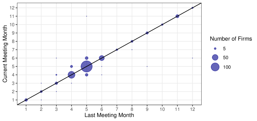
(a) AGM Months in 2019 and 2020

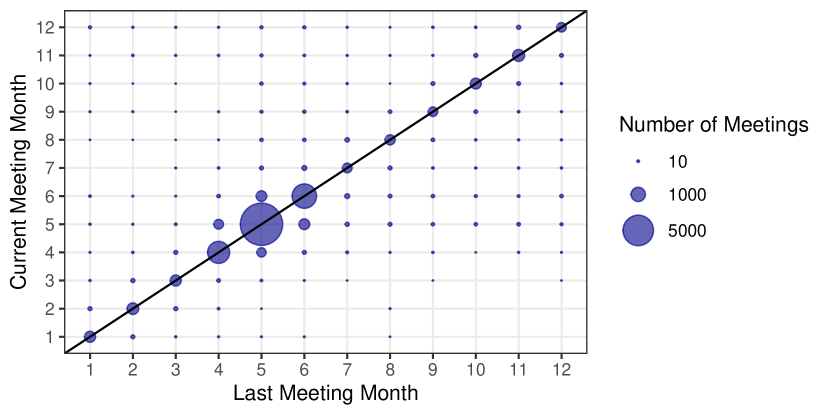
(b) AGM Months between 2012 and 2019

Note: Both panels count the occurrences of the AGM month over two adjacent years. A dot in position (2,3) means that at least one firm with an AGM in March of year $t$ had an AGM in February of year $t-1$. The size of the blue dot refers to the number of firms. Dots on the diagonal solid line indicate firms that did not change AGM month over time. Panel (a) focuses on the first six months of 2020, while Panel (b) focuses on all years between 2012 and 2019. In the last case, observations are at the firm-by-year level as firms have more than one AGM.

Figure B2: Examples of prominent shareholders featured on the media during AGMs

(a) Walton family members for Walmart

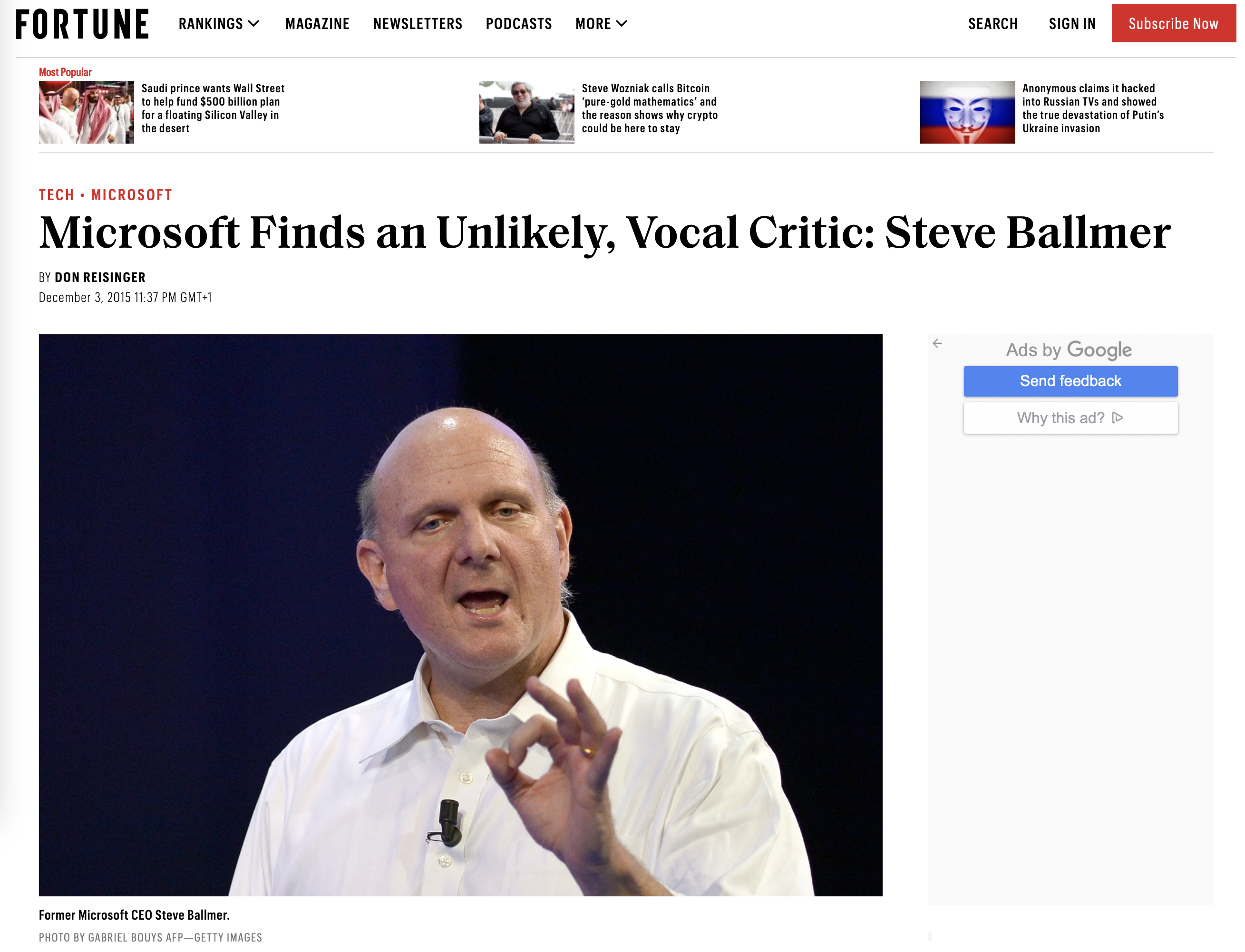
(b) Steve Ballmer for Microsoft

Note: The source for Panel a is https://www.nbcnews.com/business/business-news/wal-marts-annual-meeting-dogged-investor-anger-flna808050. The source for Panel b is https://fortune.com/2015/12/03/microsoft-critic-steve-ballmer/

Note: The figure highlights the spatial and temporal correlation between the cumulative number of covid cases (first row), deaths (second row), and donations of S&P 500 companies (third row). Each column reports the breakdown for each variable across US states on February 29 (Column 1), March 31 (Column 2), and April 15 (Column 3), when our sample ends. States in white do not house S&P 500 firms. Covid rates come from Johns Hopkins University. Donation data are hand-collected using various online sources.

Figure B4: Google Trends scores for individual and institutional blockholder

(a) Shareholders holding more than $1\%$ of a firm’s equity

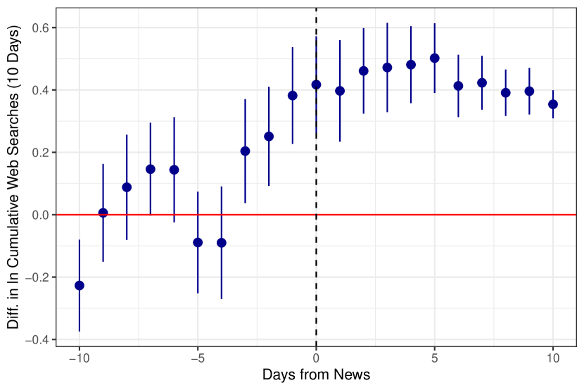
(b) Shareholders holding more than $5\%$ of a firms’s equity

Note: This figure presents results consistent with Figure 2 in the main text, but cumulating Google Trends scores over two weeks instead of 10 days. The panels show the difference in cumulative scores of individual and institutional shareholders around a donation event. The regression is detailed in Section 4.3.2. Appendix Table LABEL:tab:google reports the coefficient estimates. Standard errors are clustered by firm-by-shareholder type (bank, company, individual, financial company, government, hedge fund, insurance, mutual fund, self-control) and presented in parenthesis.

Figure B5: Abnormal and cumulative abnormal returns - event study

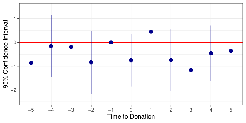
(a) Abnormal returns (AR)

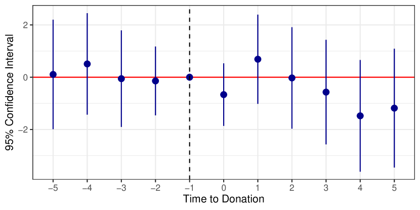
(b) Cumulative AR over five days (CAR)

Note: This figure suggests that firms do not choose to donate to improve their performance on the stock market. Panel a plots abnormal returns (ARs) while Panel b plots cumulative abnormal returns (CARs) computed using the methodology outlined in Section 4.4. Date 0 is the date when the donation was made public. All coefficients are relative to the AR or CAR computed for the day before the donation event. We report the event study for a five-day window around the donation announcement. Appendix Table A4 shows that the analysis is robust to various definitions of ARs and CARs and to various lengths of the event study interval.

Figure B6: Sales or costs: What drove productivity down during the Covid crisis?

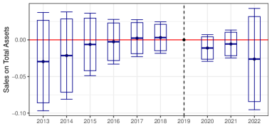
(a) Sales on total assets

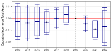
(b) Operating Income on total assets

Note: The figure reports the estimated coefficients from an event study as in (8), with sales on total assets as the dependent variable in Panel (a) and operating income on total assets in Panel (b). We report only the estimated coefficients of interest – the interaction between the time dummies and a dummy equal to one if the firm has an AGM in the 90 days after the onset of the emergency and the share of individual shareholders with more than 5% equity shares. Each regression also includes controls and firm-, time-, and time-by-industry-fixed effects as described in Section 5. The dataset considers the largest 1,000 US-listed firms. Standard errors are clustered at the state and industry levels. Error bars (boxes) report the 95% (90%) CI. Vertical dashed lines indicate the time of the event.

Figure B7: Cash imbalances due to shareholders’ rent-extraction during covid

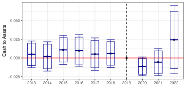
(a) Cash holdings on total assets

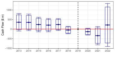
(b) Cash flows

Note: The figure reports the estimated coefficients from an event study as in (8), with cash holdings on total assets as the dependent variable in Panel (a) and cash flows on total assets in Panel (b). We report only the estimated coefficients of interest – the interaction between the time dummies and a dummy equal to one if the firm has an AGM in the 90 days after the onset of the emergency and the share of individual shareholders with more than 5% equity shares. Each regression also includes controls and firm-, time-, and time-by-industry-fixed effects as described in Section 5. The dataset considers the largest 1,000 US-listed firms. Standard errors are clustered at the state and industry levels. Error bars (boxes) report the 95% (90%) CI. Vertical dashed lines indicate the time of the event.

Figure B8: Investments dropped at treated manufacturing firms

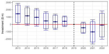
(a) All sectors

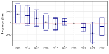
(b) Excluding service sectors

Note: The figure reports the estimated coefficients from an event study as in (8), with total invested capital as the dependent variable. Panel (a) shows the average effect in the whole sample (1,000 firms). Panel (b) excludes firms in service sectors (health care, financial, telecommunication services, utilities, real estate – 549 firms in total). We report only the estimated coefficients of interest – the interaction between the time dummies and a dummy equal to one if the firm has an AGM in the 90 days after the onset of the emergency and the share of individual shareholders with more than 5% equity shares. Each regression also includes controls and firm-, time- and time-by-industry-fixed effects as described in Section 5. The dataset considers the largest 1,000 US-listed firms. Standard errors are clustered at the state and industry levels. Error bars (boxes) report the 95% (90%) CI. Vertical dashed lines indicate the time of the event.

Figure B9: The Equity to Asset ratio dropped for the Covid case only

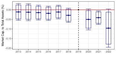
(a) Covid

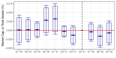
(b) Russia-Ukraine

Note: The figure reports the estimated coefficients from an event study as in (8) with market capitalization on total assets as the dependent variable. Panels (a) and (b) focus on the covid and the Russia-Ukraine cases, respectively. We report only the estimated coefficients of interest – the interaction between the time dummies and a dummy equal to one if the firm has an AGM in the 90 days after the onset of the emergency and the share of individual shareholders with more than 5% equity shares. Each regression also includes controls and firm-, time- and time-by-industry-fixed effects as described in Section 5. The dataset in Panel (a) considers the largest 1,000 US-listed firms and that in Panel (b) considers the largest US-listed firm with a positive revenue share from Russia (1,153 firms). Standard errors are clustered at the state and industry levels. Error bars (boxes) report the 95% (90%) CI. Vertical dashed lines indicate the time of the event.

Figure B10: Monotonic transformations of operating income – Russia-Ukraine

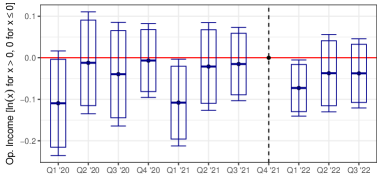
(a) $\ln(\textnormal{Op. In.})$ if OP. In. $>0$, 0 otherwise

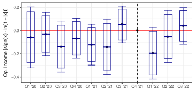
(b) $sign(\textnormal{Op. In.})\cdot\ln(1+|\textnormal{Op. In.}|)$

Note: The figure reports the estimated coefficients from an event study as in (8), with a monotonic transformation of operating income (OI) as the dependent variable. Panel (a) takes the log of OI for positive values of OI and 0 for values of OI less or equal to zero. Panel (b) takes $sign(OI)\cdot\ln(1+|OI|)$. We report only the estimated coefficients of interest – the interaction between the time dummies and a dummy equal to one if the firm has an AGM in the 90 days after the onset of the emergency and the share of individual shareholders with more than 5% equity shares. Each regression also includes controls and firm-, quarter-by-year- and quarter-by-year-by-industry-fixed effects as described in Section 5. As in Panel (b) of Figure 5 in the main text, the coefficient for Q1 2022 is statistically significant at 10% level in both panels. Its magnitude can be interpreted as a 7.4% (p-value $=$ 0.036) drop compared to the average value of the transformed OI in Panel (a) and 6.5% (p-value $=$ 0.086) for the transformation in Panel (b). The dataset considers the largest US-listed firms with a positive revenue share from Russia (1,153 firms). Standard errors are clustered at the state and industry levels. Error bars (boxes) report the 95% (90%) CI. Vertical dashed lines indicate the time of the event.

Figure B11: Sales or costs: What drove productivity down in the Russia-Ukraine case? Service sectors are excluded

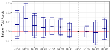
(a) Sales on total assets

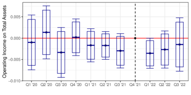
(b) Operating income on total assets

Note: The figure reports the estimated coefficients from an event study as in (8), with sales on total assets as the dependent variable in Panel (a) and operating income on total assets in Panel (b). We exclude firms in non-manufacturing sectors like health care, financial, telecommunication services, utilities, and real estate. As a result, the number of firms is 511 and 512 in Panels (a) and (b), respectively. We report only the estimated coefficients of interest – the interaction between the time dummies and a dummy equal to one if the firm has an AGM in the 90 days after the onset of the emergency and the share of individual shareholders with more than 5% equity shares. Each regression also includes controls and firm-, quarter-by-year- and quarter-by-year-by-industry-fixed effects as described in Section 5. The dataset considers the largest US-listed firm with a positive revenue share from Russia (1,153 firms). Standard errors are clustered at the state and industry levels. Error bars (boxes) report the 95% (90%) CI. Vertical dashed lines indicate the time of the event.

Figure B12: Rushing out of Russia: sales of investments and cash holdings

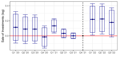
(a) Sales of investments

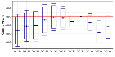
(b) Cash to Assets ratio

Note: The figure reports the estimated coefficients from an event study as in (8), with the sale of investments (log) and the ratio between cash holdings and total assets as dependent variables in Panels (a) and (b), respectively. We report only the estimated coefficients of interest – the interaction between the time dummies and a dummy equal to one if the firm has an AGM in the 90 days after the onset of the emergency and the share of individual shareholders with more than 5% equity shares. Each regression also includes controls and firm-, time- and time-by-industry-fixed effects as described in Section 5. The dataset considers the largest US-listed firm with a positive revenue share from Russia (1,153 firms). Standard errors are clustered at the state and industry levels. Error bars (boxes) report the 95% (90%) CI. Vertical dashed lines indicate the time of the event.

Figure B13: The impact of shareholders’ voice on earnings per share

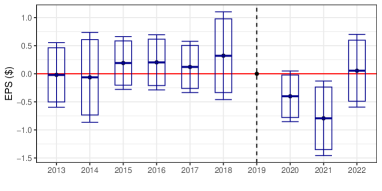
(a) Earnings per share (EPS) -
Covid case

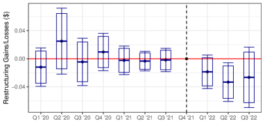
(b) Restructuring costs basic EPS effect -
Ukraine-Russia case

Note: The figure reports the estimated coefficients from an event study as in (8). The dependent variable is the EPS inclusive of the extraordinary items ($) in Panel (a) and the sum of all basic EPS effect items reported that correspond to restructuring costs in Panel (b), respectively. These costs include Chapter 11 reorganization costs and expenses, closing costs, exit costs, reductions in workforce, and relocation charges. Special item income/gains are positive an special item expenses/losses are negative. We report only the estimated coefficients of interest – interaction between the time dummies and a dummy equal to one if the firm has an AGM in the 90 days after the onset of the emergency and the share of individual shareholders with more than 5% equity shares. Each regression also includes controls and firm-, time- and time-by-industry-fixed effects as described in Section 5. The dataset in Panel (a) considers the largest 1,000 US-listed firms and that in Panel (b) considers the largest US-listed firm with a positive revenue share from Russia (1,153 firms). Standard errors are clustered at the state and industry levels. Error bars (boxes) report the 95% (90%) CI. Vertical dashed lines indicate the time of the event.

Appendix C Public Scrutiny Increases During AGM Periods

This section investigates the claim that a firm’s AGM increases its media exposure and coverage of ESG-related events by showing that news coverage of NGO campaigns against a firm increases during AGM periods.

NGO reports data. We employ data from Sigwatch, a European consulting firm tracking and analyzing NGO campaigns globally (Hatte and Koenig, 2020). A campaign is defined as an event launched by an NGO against one or several companies on a given topic. The dataset indicates the date when a campaign has been made public on an NGO’s website, the targeted company, its cause (e.g., “GMOs in food”), a measure of the sentiment ranging from –2 to +2, and the prominence of the firm in the campaign. We keep only campaigns targeting US-headquartered listed firms with a negative tone (sentiment $<0$), where only one firm is mentioned, and the mention appears in the headline (prominence = 4). We are left with 1,036 NGO reports from January 2010 to December 2019. Figure C1 shows the number of NGO campaigns annually.

News data. Firm-level news data come from Ravenpack. We keep only news with a relevance score of at least 75%. Due to our interest in AGMs, we consider only US-listed firms from 2010 to 2020 (4,676 firms) and aggregate the number of news by firm and week. The average number of weekly news for the firms in our sample is 12.7.

Figure C1: NGO campaigns per year

	Log Number of News
	(1)		(2)
NGO	0.078	∗	0.066
	(0.046)		(0.048)
Proximity to AGM	0.260	∗∗∗	0.251	∗∗∗
	(0.009)		(0.009)
NGO $\times$ Proximity to AGM	0.383	∗∗	0.406	∗∗
	(0.168)		(0.170)
Lag Log Number of News			0.009	∗∗∗
			(0.0008)
Firm fixed effects	✓		✓
Week fixed effects	✓		✓
$N$	1,426,313		1,373,729
Adjusted R-squared	0.3938		0.3940
* – $p<0.1$; ** – $p<0.05$; *** – $p<0.01$.

Table C1: Media attention around AGMs

Note: The figure displays the yearly count of NGO campaigns targeting a company listed in the US from January 2010 to December 2019 (1,036 campaigns). The table presents the OLS regression coefficients from (C1). NGO is a dummy equal to one if firm $f$ has been targeted by a negative NGO report during the current week. For firm $f$ in week $w$ Proximity to AGM is close to zero if firm $f$’s yearly AGM is far away from week $w$ and is 1 if, instead, its AGM is in week $w$. The regression includes firm- and week-fixed effects. The sample period goes from January 2010 to December 2019. Standard errors are clustered at the level of the firm and are reported in parentheses.

Analysis. Figure C2 shows that news coverage grows during AGM periods for each year. To assess how the AGM period affects media exposure, we estimate:

$$\text{News}_{fw} =\beta_{0}\text{NGO}_{fw}+\beta_{1}\text{Proximity to AGM}_{fw}$$ (C1)

$$+\beta_{treat}\text{NGO}_{fw}\times\text{Proximity to AGM}_{fw}+\alpha_{f}+\tau_{w}+\epsilon_{fw},$$

where News_fw is the log number of news about firm $f$ in week $w$ plus one, NGO_fw is equal to one if a negative NGO report has been published about firm $f$ during week $w$, and Proximity to AGM_fw is the inverse of one plus the distance (in weeks) to the nearest AGM. Therefore, for firm $f$ in week $w$ Proximity to AGM_fw is close to zero if firm $f$’s yearly AGM is far away from week $w$ and is one if, instead, its AGM is in week $w$ and zero otherwise. The regression includes firm- and week-fixed effects. Table C1 finds that firms receive more media exposure around the time of their AGM, as shown by the positive and statistically significant coefficient on the Proximity to AGM_fw variable (second row). The coefficient on the interaction term confirms that ESG-related events receive more coverage as the distance between AGM and NGO campaigns shrinks. The result survives even after controlling for firm- and time-varying effects captured by the lagged dependent variable (Column 2). Therefore, the analysis indicates that the AGM period intensifies media coverage. These results are consistent with Figure C4 that shows that NGOs scrutiny increases during a firm’s AGM period.

Figure C2: Greater media coverage around AGM periods (red) than in other periods (blue)

(a) AGM Period defined as Within 10 Days

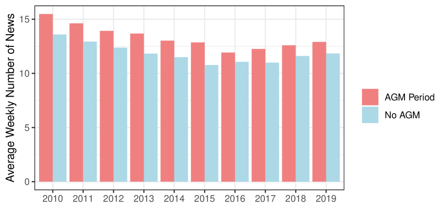
(b) AGM Period defined as Within 3 Months

Note: News coverage is much higher during AGM periods (red bars) than during other periods (blue bars). Extending the AGM period from a window of $\pm$ ten days (Panel a) to $\pm$ three months (Panel b), the distance between the two columns decreases, as the gap between news coverage during AGM periods and other periods is washed out by a greater interval. News data come from Ravenpack. AGM dates come from ISS.

Attention decay. How long does the AGM effect last? We modify (C1) by redefining the variable Proximity to AGM_fw and let it be 1 if week $w$ is within $\pm k$ weeks from an AGM and 0 otherwise. We vary $k$ between 1 and 24 weeks: Figure C4 plots the estimated $\beta_{treat}$ coefficients of the 24 regressions obtained by varying this variable in (C1) and the corresponding 95% confidence intervals. We find that news coverage increases with proximity to an AGM. The additional media coverage due to an AGM period is instead statistically indistinguishable from 0 when we consider AGM periods greater than 11 weeks, or over three months.

Conclusion. In summary, this analysis indicates that ESG-related events receive significantly more media coverage when they happen closer to an AGM. If the AGM is far in time, i.e., further than three months, these events do not benefit from the greater media attention that firms face during their AGM periods. Drawing a parallel with our analysis in the main text, the largest possible distance between the date of inclusion into the treatment (January 15, 2020) and the date of the latest possible AGM of a treated firm (April 15, 2020) is exactly three months. Thus, the distance between AGMs and donations must be smaller than three months for treated firms. To the extent that the empirical evidence on NGO campaigns translates to corporate donations, this analysis indicates that the AGM treatment successfully intensifies the media coverage of a firm’s donations.

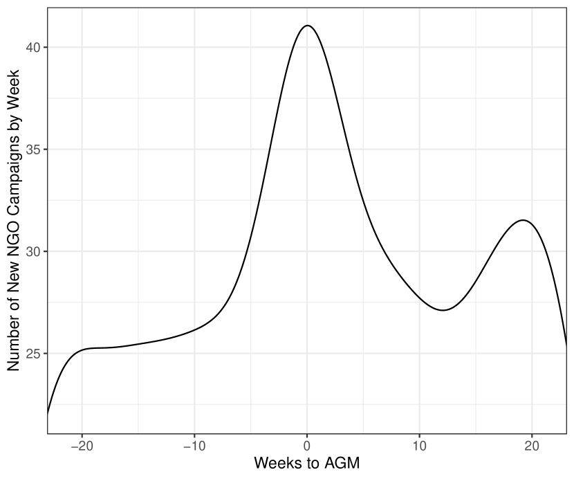
Figure C3: Public scrutiny during AGMs

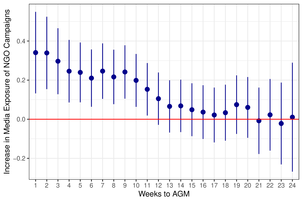
Figure C4: Decay of media exposure

Note: Figure C4 plots the density of NGO campaigns relative to the closest AGM dates of the targeted firms using pre-pandemic data from January 2010 to December 2019. The sample covers 4,676 US-listed firms and 1,036 high-severity NGO campaigns. The x-axis re-calendarizes time so that, for each year and firm, week 0 is the AGM week for all firms. Figure C4 presents the beta coefficients from multiple regressions. Each coefficient comes from regressing the log of one plus the number of news about firm $f$ in week $w$ on a dummy indicating the publication of a negative NGO report about firm $f$ in week $w$, a dummy equal to one when week $w$ is less than $k$ weeks away from the nearest AGM, where we take $k$ to vary between 1 and 24 weeks, the interaction between these two dummy variables, and firm and week fixed effects. The figure reports the estimated interaction term as we vary $k$ on the x-axis. The figure also reports the 95% confidence interval when the standard errors are clustered at the level of the firm. The sample period goes from January 2010 to December 2019 and covers 4,676 firms.

Appendix D Main Results with Alternative Datasets

The analyses in Section 4 use both financial and ownership data from Orbis, where, however, data for a few firms are missing. This section shows that the main results from that section are robust by drawing ownership data from another source, Refinitiv. The following exhibits present the analyses from Figure 1 and Tables 2 and 3 using the Refinitiv Consolited Ownership dataset. All the variables are defined as in Section 4.

Despite the different and slightly larger dataset, we find very similar results to those presented in the main text. Figure D1 reports the coefficients from the event study in (3), which regresses whether a firm donated for covid before April 2020 on dummies indicating whether the firm held an AGM in the weeks between January 15 and June 15, 2020. As in Figure 1, only firms with individual shareholders (blue circles) are associated to a greater probability of donating. The difference between red triangles and blue dots is evident across the columns of Table D1, which estimates coefficients that are almost identical to those in the main text. Finally, D2 finds that the correlation between the donations of a financial shareholder and the firms in its portfolio is negative (and statistically significant) for blockholding shares ($\geq 2\%$).

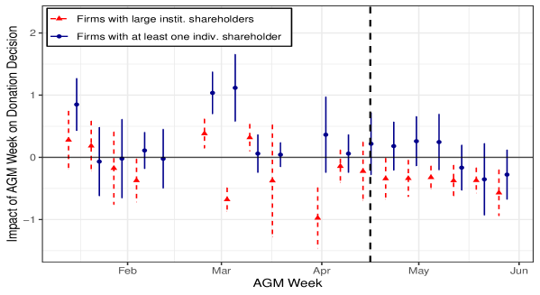
Figure D1: Influence on donations by AGM week and shareholder composition - different shareholding data

Note: The figure plots the estimated coefficients of an event study regressing whether a firm donated between January and April 2020 on dummies indicating whether the firm held an AGM in the weeks between January 15 and June 15, 2020. Compared to Figure 1, this table uses ownership data from Refinitiv instead of Orbis. The reference period is the week of June 15, 2020. Coefficients shown in circles are estimated using a sample of firms with at least one individual shareholder with at least 0.1% shares, and the triangles are from a sample of firms whose institutional blockholding (shareholders owning at least 5% a firm’s equity as of December 2019) is greater than the median at S&P 500 firms. The vertical dashed line is on April 15, 2020, 90 days after the first US covid case.

Table D1: Shareholders’ influence on covid donations - different shareholding data

	Whether Firm $f$ has Donated (0/1)
	(1)		(2)		(3)		(4)		(5)		(6)
Ownership	-0.0092		0.0003		-0.0140		-0.0181		-0.0880	∗∗∗	0.0432	∗
	(0.0138)		(0.0128)		(0.0397)		(0.0276)		(0.0207)		(0.0209)
AGM	0.1104		0.1118		0.0809		0.1084		0.1143		0.1335
	(0.1244)		(0.1254)		(0.1345)		(0.1167)		(0.1287)		(0.1200)
Ownership $\times$ AGM	0.0808	∗∗	0.0828	∗∗	0.0574		-0.1664	∗∗	0.0013		-0.0846
	(0.0255)		(0.0265)		(0.0644)		(0.0667)		(0.0643)		(0.1361)
Ownership is defined as	Individuals						Institutional
Ownership is the shares of investors owning:	$>10\%$		$>5\%$		$(0\%,2\%)$		$>10\%$		$>5\%$		$(0\%,2\%)$
Industry fixed effects	✓		✓		✓		✓		✓		✓
State fixed effects	✓		✓		✓		✓		✓		✓
Observations	482		482		482		482		482		482
Adjusted R-squared	0.2165		0.2166		0.2150		0.2208		0.2389		0.2184
* – $p<0.1$; ** – $p<0.05$; *** – $p<0.01$.

• Note: The table presents the coefficients from OLS regressions of an indicator variable that is one if firm $f$ has donated by April 15, 2020, on covariates. Compared to Table 2, this table uses ownership data from Refinitiv instead of Orbis. Italicized variables are defined in the middle panel. The variable Ownership is the share of either individual (Columns 1-3) or institutional investors (Columns 4-6) among all investors owning at least a share of total equity, as defined in the middle panel. Institutional investors include the largest financial investors in Table 1, namely, banks, mutual funds, and insurance firms. The variable Ownership is standardized. The AGM variable is an indicator variable taking value one if the firm has an AGM before April 15, 2020, and zero otherwise. All columns include industry- and state-fixed effects. Robust standard errors in parenthesis.

Table D2: Correlation of donations of financial shareholders’ and their portfolios

	Spearman Correlation
Minimum	Weighted Average
Equity Share	$\times$ AGM
Considered	[p-values]
(1)	(2)
0%	-0.082
(Avg. $N$ = 374)	[0.668]
1%	0.073
(Avg. $N$ = 75)	[0.840]
2%	-0.933
(Avg. $N$ = 60)	[0.007]
3%	-0.889
(Avg. $N$ = 66)	[0.044]
4%	-0.889
(Avg. $N$ = 81)	[0.044]
5%	-0.943
(Avg. $N$ = 52)	[0.057]

• Note: This table shows a negative correlation between large institutional investors such as financial firms in the S&P 500 Index and the firms in their portfolio that had their AGMs before April 15, 2020. Compared to Table 3, this table uses ownership data from Refinitiv instead of Orbis. The negative correlation indicates that financial investors opposed COVID-19-related donations in their footprints. The table computes the Spearman correlation between whether a financial firm donates and the share of donations at the firms in its portfolio. In each row, we vary the minimum share % that a firm must have in another firm to be considered an investment according to the percentages reported in the first column. Column 1 also reports the average number of S&P500 firms in the portfolio of a financial investor in parenthesis. Column 2 considers only investments that got an AGM in the period under consideration (i.e., $\sum_{j}share_{ij}\times\mathbb{I}_{[\text{firm }j\text{ donated}]}\times\mathbb{I}_{[i\text{'s share in }j\text{ is greater than }x\%]}\times\mathbb{I}_{[j\text{ has an AGM}]}$). p-values testing whether the Spearman correlation is equal to zero are reported in square brackets.

Appendix E Private Sanctions on Russia

This section focuses on shareholder influence after Russia invaded Ukraine in February 2022 as an external validity exercise for the mechanism exposed in the main text.

E.1 Background and Data

On February 24, 2022, Russia started the so-called “special military operation.” We take this date as the beginning of our sample. Sonnenfeld et al. (2022) list firms exposed to the Russian economy (e.g., exporters to Russia) that took a pro or against position vis-á-vis Russia.

Data construction. We accessed this list on March 23, a month after the beginning of the invasion. The list contains 476 international firms operating in Russia at the time. Figure 1(a) shows a breakdown of this sample based on different firm categories. Most of the observations belong to non-US firms (especially from the UK, Germany, and France) and international sports federations (e.g., UEFA), which quickly denied access to Russian sports teams in the days after the beginning of the invasion. We exclude these firms since our exogenous variation is based on the SEC rules and ISS requirements. Excluding another 12% of the observations that account for US non-listed firms for which we lack shareholding data, we are left with 164 US-listed firms for which the 2022 AGM date is available on the Refinitiv database. This dataset is not the whole universe of US-listed firms operating in Russia but a collection of the firms that took actions, either pro or against Russia, in the first month of the war. By taking early actions, this dataset spans the firms that are most exposed to Russia, and thus, these firms are the most relevant for our analysis. 85% of the firms in this list have a market capitalization above $8bn, which is the limit for inclusion in the S&P 500 index.

Classification of firms’ decisions. Sonnenfeld et al. (2022) categorizes firms as: (1) Grade A - Surgical Removal, Resection (51 firms) for firms that left Russia; (2) Grade B – Keeping Options Open for Return (69 firms) for firms that paused their ongoing projects; (3) Grade C – Reducing Current Operations (9 firms), for firms that paused certain operations; (4) Grade D – Holding Off New Investments/Development (27 firms), for firms that halted future investments; (5) Grade F – Defying Demands for Exit or Reduction of Activities (9 firms), for firms that kept working in Russia.

Data summary. Among the 164 firms in our database, 94 had an AGM in the three months following the outbreak of the war, whereas the 70 remaining firms had AGMs in another period. Table E2 shows summary statistics comparable to those in Table 1 of the main text for the two groups. Column 3 performs balance checks over observable variables such as market capitalization, revenues, net income, fraction of revenues coming from the US and Canada, age of the CEO, ESG scores, average brokers’ recommendations, and shareholding. Overall, control (treatment) firms are more represented in Grade A (D). The remaining two columns illustrate the variation in Grade across firms with at least 2% of individual shareholders or with at least 5% of institutional shareholders. Finally, Figure 1(b) shows that, within sectors, firms are almost evenly distributed between treatment (blue) and control firms (red) – this further corroborates the exogeneity of selection into treatment.

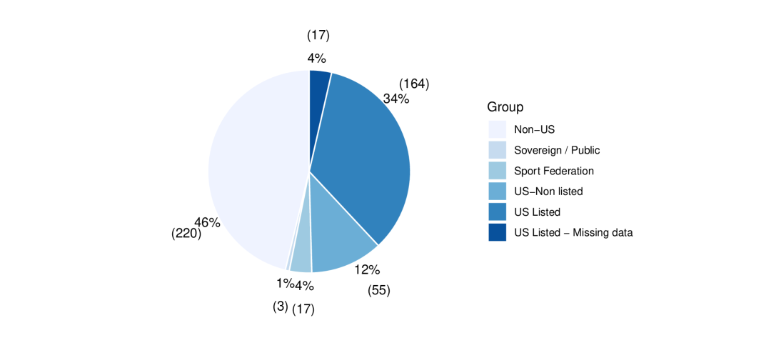
(a) Surveyed firms

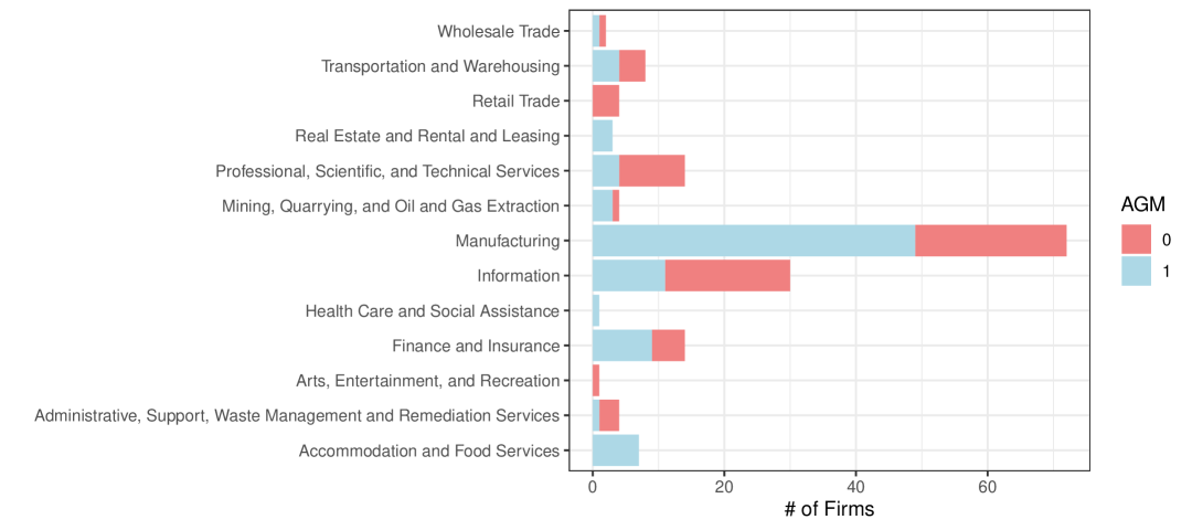
(b) Industry breakdown

Note: Panel (a) 34% of the firm surveyed in Sonnenfeld et al. (2022) are U.S.-listed firms. Panel (b) Number of firms by sector. Red (light blue) bars indicate control (treatment) group firms. Firms with a 2022 AGM scheduled between February 24 and May 24, 2022, are in the treated group as they have an AGM in the three months after February 24.

E.2 Robustness Checks

Below, we present several robustness checks for the analysis in Section 4.5.1, which employed (2) to study whether firms with greater shares of large individual (institutional) blockholders support (oppose) exiting Russia. Arguably, outright exit is the highest possible sanction that firms can take against Russia, and it was not forced by international sanctions at the time. Of course, the optimal action might vary across sectors, as, for instance, internet firms might prefer to stay in Russia to disseminate Western information. For this reason, we exclude Grade F firms from the main analysis and include industry-fixed effects and several covariates. Almost all firms have institutional blockholders with holdings greater than 2%; therefore, to properly capture individual shareholder’s voice, we control for a dummy that is one if firm $f$ has above the median blockholding of institutional investors and zero otherwise when $\textnormal{Ownership}_{f}$ refers to individual investors. This additional variable accounts for the fact that large institutional blockholders might reduce the effectiveness of individual shareholder voices, as shown in Section 2. Allowing for different intercepts based on shareholder composition ensures the identification of the coefficient of interest, $\beta_{treat}$.

Note. Because of space constraints, we report the full regression tables only for selected analyses. For the others, we only discuss the results, which are available upon request.

Measuring large blockholding. Tables 4 from the main text measures the association between a firm and its largest shareholders with a variable that is 1 if a firm has above the median value of blockholding of a specific shareholder reference group with at least a $x\%$ share and zero otherwise. We then vary $x$ across columns to be greater than 10%, 5%, or 2%. If we used the underlying continuous variable instead, namely, the share of a certain group of shareholders (e.g., individuals) with at least a $x\%$ share, our results would not vary qualitatively.

Which institutional blockholders opposed exits? To better highlight the role of prominent shareholders in opposing exit decisions, we run the same analysis in (2) using $\textnormal{Above Median Blockholding}_{f}$ as a measure of the association of a firm to its main shareholders. As in Section 4.5.1, this variable is 1 if the firm has above the median value of blockholding of a specific shareholder reference group with $x\%$ share and 0 otherwise. Table E3 finds that mutual funds blockholders play the most important role, followed in order by banks and insurance companies, which is consistent with what we reported for the pandemic in Appendix Table LABEL:tab:reg-results-large-shareholders. This is probably because mutual funds are the largest shareholders in these firms (Table E2), and they might be following their investments more actively than other investors due to their statutes.

Including Grade F firms. Excluding firms that announced that they would not exit Russia does not materially change our results. For instance, unreported analyses find that $\beta_{treat}$ is 0.656 (S.E. 0.255) when the treatment group includes firms more exposed to individual shareholders with at least a 5% share and –0.320 (S.E. 0.157) for the similar analysis using institutional shareholders. These coefficients were 0.316 and –0.152 Table 4, which run the same analyses excluding the nine Grade F firms.

Excluding airline companies. Airline companies’ decisions could be driven by Russia’s ban on Western carriers from flying over the country. Excluding airline companies (3 observations: American Airlines, Delta Airlines, and United Airlines) does not change our results qualitatively.

Only S&P 500 firms in the list. Firms could be quite heterogeneous, and the decisions of small firms might not receive the same coverage as that of large firms. Excluding firms that are not on the S&P 500 list does not change our results qualitatively despite reducing the sample size to 103 observations only.

All S&P 500 firms. Selection might bias our analysis, as we do not observe the whole set of firms that deal with Russia but only a subset. To tackle this issue, we run (5) as described above on all U.S.-listed S&P 500 firms. Since the firms that do not have business dealings with Russia will not make any decisions, we subset the dataset to consider only the firms whose exposure to Russia is greater than the median value observed among S&P 500 firms. Consistently, we find that the firms most exposed to large individual shareholders are most likely to exit Russia.

A different specification. The proposed regressions focus either on institutional or individual shareholders, while firm decisions might result from pressure from different shareholders. To account for this circumstance, we update (5) as follows:

$$\textnormal{Exit}_{f} =\tilde{\beta}_{0}+\tilde{\beta}_{1}\textnormal{AGM}_{f}$$

$$+\gamma_{1}\textnormal{Above Median Indiv. Block.}_{f}+\gamma_{2}\,\textnormal{Above Median Indiv. Block.}_{f}\times\textnormal{AGM}_{f}$$

$$+\theta_{1}\textnormal{Above Median Instit. Block.}_{f}+\theta_{2}\,\textnormal{Above Median Instit. Block.}_{f}\times\textnormal{AGM}_{f}$$

$$+\tilde{\beta}_{2}\textnormal{X}_{f}+\tilde{\varepsilon_{f}},$$ (E1)

where the coefficient vectors $\{\gamma_{i}\}_{i=1}^{2}$ and $\{\theta_{i}\}_{i=1}^{2}$ refer to either individual or institutional blockholders above the median level. Therefore, this specification simultaneously accounts for the effect of the treatment on both types of shareholders. The remaining variables stay unchanged. Table E4 reports the results varying the thresholds of the blockholder definition and whether the reference institutional shareholders are all institutional shareholders (Columns 1 to 4) or only mutual funds (Columns 5 to 8). Overall, the results are in line with those presented in the previous analyses, not only in terms of the sign of the coefficients but also in terms of their magnitude: a shareholder’s voice grows as the blockholding threshold increases.

Financials in 2022. Exit from Russia could be rather expensive, pushing firms with bad financial outcomes in 2022 to stay in Russia.For instance, Shell communicated that its exit from Russia would cost between $4bn and $5bn. However, first, whether a firm had negative financial results is orthogonal to the timing of the AGM. Second, unreported results indicate that having a negative net income is not associated with Grade F and Grade A firms are not those with the largest profits. Similarly, Grade A firms are not the biggest and are rather comparable with Grade F firms in terms of market capitalization.

E.3 Dropping Russian Suppliers

This section extends Appendix E by considering the decision to cut supply chain relationships with Russian corporations soon after the beginning of the invasion. To that end, we identify all relationships between US and Russian firms using Factset’s Supply Chain Relationships data. We identify 102 US firms with an outstanding relationship with at least one Russian firm as of February 24, 2022, and with available shareholding and AGM data. Ninety-six also have all the control variables used in the preceding analysis available.

Table E1: Blockholders’ influence on the decision to cur supply chain relationships with Russian corporations

	Drop Relationship (0/1)
	(1)		(2)
Above Median Blockholding	-0.107		-0.380	∗∗∗
	(0.129)		(0.060)
AGM	-0.159	∗	-0.103
	(0.088)		(0.072)
AGM $\times$ Above Median Blockholding	0.152		0.456	∗∗∗
	(0.186)		(0.112)
Threshold to be considered a blockholder:	$>$0%		$>$5%
Sector FE	✓		✓
Controls	✓		✓
$N$	96		96
Adjusted R-squared	0.1928		0.2079
* – $p<0.1$; ** – $p<0.05$; *** – $p<0.01$.

• Note: This table reports considers the influence of individual blockholders on US corporations’ decision to cut relationships with Russian corporations in their supply chain after the beginning of the Ukraine invasion. It is the regression of a dummy equal to one if US firm $f$ has stopped doing business with at least one Russian firm between February 24, 2022 and May 24,2022, on a dummy equal to one if the firm has a level of individual shareholding above median (Column 1) or a level of individual blockholding ($\>5\%$) greater than the median (Column 2), a dummy indicating an early AGM (between February 24 and May 24, 2022), and the interaction between the two. The regressions also include sector fixed effects, and, as controls, the share of firm $f$’s revenue coming from operations in the US and Canada, the share of revenue coming from operations in Russia, its CEO age, net income, and a dummy indicating an above-median level of institutional ownership.

Table E2: Summary of the sample of listed firms exposed to the Russian economy by group

	(1)	(2)	(3)	(4)	(5)
	Annual General Meeting (AGM)			Individual	Institutional
	between 02/22 and 05/22		p-values	Shareholders	Shareholders
	Yes (treat)	No (control)	(1) - (2)	With $\geq$ 2%	With $\geq$ 5%
i. Firm Characteristics
Market Cap (bn USD)	109.4	186.9	0.202	129.9	143.2
Brokers’ Recommendation [-2, 2]	1.0	1.1	0.291	1.0	1.0
Revenue (bn USD)	33.2	35.1	0.849	33.8	33.5
EBIT (bn USD)	5.0	4.6	0.859	2.7	4.8
- EBIT $>$ (dummy) 0	87.1	81.7	0.352	88.9	84.3
Net Income (bn USD)	4.9	5.6	0.724	2.5	5.3
- Net Income $>$ 0 (dummy)	87.1	80.3	0.25	77.8	84.3
% of Revenues from US and Canada	51.8	51.9	0.98	51.9	52.0
CEO Age	61.6	60.4	0.337	62.1	61.0
ESG Score	71.3	66.6	0.101	63.5	69.2
ii. Shareholding (% Ownership)
Share of Individual Investors With $>$ 2%	1.4	3.3	0.15	13.6	2.0
Share of Institutional Investors With $>$ 5%	28.6	25.0	0.08	23.7	27.9
- Mutual Funds	10.1	9.6	0.746	8.1	10.2
- Banks	0.5	0.0	0.07	0.2	0.3
- Insurance	1.1	0.0	0.029	0.0	0.6
iii. Corporate Actions as of March 23, 2022 (% of each group)
Grade A - Surgical Removal, Resection (51 firms)	22.6	40.8	0.014	25.9	31.4
Grade B – Keeping Options Open for Return (69 firms)	41.9	42.3	0.968	55.6	42.1
Grade C – Reducing Current Operations (9 firms)	8.6	1.4	0.028	3.7	5.7
Grade D – Holding Off New Investments/Development (27 firms)	22.6	8.5	0.011	11.1	15.1
Grade F – Defying Demands for Exit or Reduction of Activities (9 firms)	4.3	7.0	0.462	3.7	5.7

• Note: This table compares the firms in the treatment and control groups used in the empirical analysis of the corporate sanctions against the Russian economy executed in the first month of the 2022 war in Ukraine. This data was collected by Jeffrey Sonnenfeld and his team at Yale SOM, which we thank for sharing the data and explaining the data construction. Columns 1 focuses on firms with AGM within 3 months after the start of the war and Columns 2 the other firms. Column 4 focuses on firms with at least one individual shareholder owning more than 2% of total equity. Column 6 focuses on firms with at least one institutional investor owning more than 5% of total equity. Shareholding, profitability and control variables come from Refinitiv. The variable Brokers’ Recommendation refers to the recommendations of equity analysts and it ranges between -2 and 2, where strong sell $=-2$, sell $=-1$, hold/neutral $=0$, buy $=1$, strong buy $=2$. ESG score is the Social score of the firm as computed by Refinitiv.

Table E3: Blockholders’ influence on the decision to exit the Russian market after the invasion of Ukraine - breakdown by blockholder types

	Exited Russia (0/1)
	(1)		(2)		(3)		(4)		(5)		(6)		(7)		(8)		(9)		(10)
AGM	–0.067		–0.094		0.144		0.043		–0.012		–0.022		–0.028		0.003		–0.032		0.098
	(0.090)		(0.090)		(0.115)		(0.111)		(0.085)		(0.086)		(0.090)		(0.091)		(0.089)		(0.099)
Above Median Blockholding	–0.547	∗∗∗	–0.428	∗∗∗	0.116		0.148		0.703	∗∗∗	0.423	∗∗	0.163		0.262		–0.067		0.206
	(0.181)		(0.128)		(0.132)		(0.137)		(0.193)		(0.213)		(0.264)		(0.272)		(0.181)		(0.129)
AGM $\times$ Above Median Blockholding	0.705	∗∗∗	0.263		–0.341	∗∗	–0.188		–0.584	∗∗	–0.309		–0.150		–0.332		–0.176		–0.293	∗
	(0.254)		(0.175)		(0.165)		(0.159)		(0.230)		(0.245)		(0.283)		(0.292)		(0.198)		(0.154)
Above Median Blockholding (0/1) defined for:	Individual				Institutional				Banks				Insurance				Mutual Funds
Threshold to be considered a blockholder:	$>$10%		$>$2%		$>$10%		$>$2%		$>$2%		$>$1%		$>$2%		$>$1%		$>$10%		$>$5%
Controls	✓		✓		✓		✓		✓		✓		✓		✓		✓		✓
Sector fixed effect	✓		✓		✓		✓		✓		✓		✓		✓		✓		✓
$N$	138		138		138		138		138		138		138		138		138		138
Adjusted R-squared	0.2762		0.2879		0.2642		0.2372		0.2818		0.2628		0.2280		0.2378		0.2397		0.2523
* – $p<0.1$; ** – $p<0.05$; *** – $p<0.01$.

• Note: This table indicates that banks and mutual funds mostly opposed exiting from Russia. The table reports the coefficients from OLS regressions of whether firm $f$ has exited Russia as of March 23, 2022, on (i) the AGM treatment and (ii) a dummy Above Median Blockholding for whether the shareholders of firm $f$ include blockholders with shares above the median value for that specific category, and (iii) their interaction. Categories vary across columns based on the reference shareholder type, and the minimum blockholding threshold considered and are defined in the middle panel. Firms with Grade F (i.e., firms that announced business as usual) are not included in the analysis. Institutional investors include mutual funds, banks, insurance, hedge funds, private equity, and venture capital. All columns include sector-fixed effects. Control variables include the share of revenues that come from activities in the US and Canada, brokers’ recommendations, CEO age, and net income. Market capitalization, revenues, and net income are highly correlated; controlling for any of these two variables instead of net income does not change the results qualitatively. For models where individual investors are the reference category, we also include a dummy equal to 1 for above-median institutional ownership to account for the importance of institutional blockholders among the firms in this sample, and for the impossibility of exploiting firm fixed effects with only cross-sectional variations. Robust standard errors are reported in parenthesis.

Table E4: Blockholders’ influence on the decision to exit the Russian market after the invasion of Ukraine - simultaneous effect of different blockholder types

	Exited Russia (0/1)
	(1)		(2)		(3)		(4)		(5)		(6)		(7)		(8)
AGM	0.099		–0.014		–0.011		0.015		–0.067		0.055		–0.098		–0.093
	(0.114)		(0.112)		(0.112)		(0.105)		(0.089)		(0.096)		(0.110)		(0.111)
Above Median Indiv. Block.	–0.518	∗∗∗	–0.541	∗∗∗	–0.430	∗∗∗	–0.152		–0.531	∗∗∗	–0.548	∗∗∗	–0.419	∗∗∗	–0.191
	(0.189)		(0.144)		(0.125)		(0.141)		(0.184)		(0.131)		(0.130)		(0.146)
AGM $\times$ Above Median Indiv. Block.	0.786	∗∗∗	0.335		0.271		0.099		0.658	∗∗	0.344		0.245		0.114
	(0.238)		(0.254)		(0.173)		(0.183)		(0.269)		(0.230)		(0.183)		(0.191)
Above Median Institut. Block.	0.100		0.067		0.168		0.281	∗	–0.053		0.211	∗	0.028		0.037
	(0.125)		(0.123)		(0.129)		(0.144)		(0.171)		(0.119)		(0.117)		(0.136)
AGM $\times$ Above Median Institut. Block.	–0.326	∗∗	–0.136		–0.189		–0.282	∗	–0.175		–0.292	∗∗	0.023		0.023
	(0.163)		(0.150)		(0.150)		(0.165)		(0.189)		(0.145)		(0.146)		(0.164)
Above Median Institut. Block. (0/1) defined for:	All institutional investors								Only mutual funds
Threshold to be considered a blockholder:	$>$10%		$>$5%		$>$2%		$>$1%		$>$10%		$>$5%		$>$2%		$>$1%
Sector FE	✓		✓		✓		✓		✓		✓		✓		✓
Controls	✓		✓		✓		✓		✓		✓		✓		✓
$N$	138		138		138		138		138		138		138		138
Adjusted R-squared	0.3012		0.2915		0.2921		0.2666		0.2762		0.3140		0.2799		0.2341
* – $p<0.1$; ** – $p<0.05$; *** – $p<0.01$.

• Note: This table considers the influence of large institutional and large individual blockholders simultaneously. The regression equation is presented in Equation E.2; it regresses whether firm $f$ has exited Russia as of March 23, 2022, on the (i) the AGM treatment and (ii) a dummy Above Median Indiv. Blockholding for whether the shareholders of firm $f$ include blockholders with shares above the median value for individual shareholders, (iii) their interaction, (iv) another dummy Above Median Institut. Blockholding for whether the shareholders of firm $f$ include blockholders with shares above the median value for that specific category, and its interaction with the AGM treatment. Categories vary across columns based on the reference institutional shareholder (either all institutions in Columns 1 to 4, or only mutual funds in Columns 5 to 8) and the minimum blockholding threshold considered, and are defined in the middle panel. Also, firms with Grade F (i.e., firms that announced business as usual) are included in the analysis. Institutional investors include mutual funds, banks, insurance, hedge funds, private equity, and venture capital. Control variables include the share of revenues that come from activities in the US and Canada, the exposure to Russia, brokers’ recommendations, CEO age, and net income. Market capitalization, revenues, and net income are highly correlated; controlling for any of these two variables instead of net income does not change the results qualitatively. All columns include sector-fixed effects. Robust standard errors are reported in parenthesis.

Appendix F Data on Donations and ESG between 2011-2021

This section describes the data used in Section 4.5.2. We gather donation news from Ravenpack by selecting all news in the “donation” category with a positive event sentiment for all U.S. firms, subsetting firms with an “entity relevance” score above 75%. The sample covers 2011 to 2021. We started from the whole universe of firms in Compustat covered by RepRisk during the whole sample period (2,722 firms). We kept firms listed on the NYSE or the NASDAQ and headquartered in the US, with no missing data in Compustat and in ISS, and whose Refinitiv ESG scores, historical shareholding data (the Refinitiv Ownership Database) were available. This narrows down the sample to 988 firms, accounting for 90% of the market capitalization of the original sample.

Table F1 provides summary statistics on the market capitalization, number of ESG risk incidents, ownership data, and ESG scores for the companies in the sample. The average market capitalization is 53 billion dollars, ranging from 1 million to 1.7 trillion. Firms have, on average, 772 reported adverse ESG news (“ESG incidents”) during the period. Equivalently, a firm has a 30% chance of observing news in a given month. The summary statistics emphasize the holdings of individual and financial (“institutional”) investors, which include Banks and Insurance Companies. ESG scores are expressed as a percentage, are scaled by industry and typically vary once a year.

Table F1: Summary statistics of ESG data from 2011 to 2021

	Mean	Median	25%	75%	s.d.
	(1)	(2)	(3)	(4)	(5)
Market Capitalization (m USD)	21,269	4,831	1,553	16,192	60,631
RepRisk Incidents & Donations Data
Number of Incidents	772.4	96	0	594	1,889.2
Number of E-Incidents	188.7	12	0	96	611.3
Number of S-Incidents	651.4	84	0	498	1,616.6
Number of G-Incidents	129.9	6	0	60	448.9
Probability of Having a High-Severity S-Incident (%)	4.5	0	0	0	27.3
Number of Donations	4.5	2	1	5	7.4
Ownership Data
Individual Investor Ownership (%)	2.7	0	0	0.7	9.9
Institutional Ownership (%)	43.8	35.6	16.0	55.1	70.3
ESG Scores Data
Environmental Score (%)	52.6	55.8	34.0	74.0	25.9
Social Score (%)	42.7	45.4	9.4	71.0	31.2
Governance Score (%)	54.4	58.1	37.8	75.1	25.7

• Note: Summary statistics of the ESG Refinitiv news coverage data. Shares are computed over total equity. Institutional Owernship is the sum of the shares owned by Banks, Hedge Funds, Insurance Companues, Investment Advisors, Mutual Funds, Pension Funds, Private Equity, and Venture Capital firms. Risk Incidents data report the number of incidents observed by firms during the whole sample period.

References

- Admati and Pfleiderer (2009) Admati, A. R. and Pfleiderer, P. (2009). The “wall street walk” and shareholder activism: Exit as a form of voice. The Review of Financial Studies, 22 (7), 2645–2685.
- Aghion and Tirole (1997) Aghion, P. and Tirole, J. (1997). Formal and real authority in organizations. Journal of political economy, 105 (1), 1–29.
- Akey et al. (2021) Akey, P., Lewellen, S., Liskovich, I. and Schiller, C. (2021). Hacking corporate reputations. Rotman School of Management Working Paper, (3143740).
- Allcott et al. (2022) Allcott, H., Montanari, G., Ozaltun, B. and Tan, B. (2022). An economic view of corporate social impact. Available at SSRN 4047276.
- Ananthakrishnan et al. (2023) Ananthakrishnan, U., Proserpio, D. and Sharma, S. (2023). I hear you: Does quality improve with customer voice? Marketing Science.
- Andreoni (1989) Andreoni, J. (1989). Giving with impure altruism: Applications to charity and Ricardian equivalence. Journal of political Economy, 97 (6), 1447–1458.
- Ashraf and Bandiera (2018) Ashraf, N. and Bandiera, O. (2018). Social incentives in organizations. Annual Review of Economics, 10, 439–463.
- Azar et al. (2018) Azar, J., Schmalz, M. C. and Tecu, I. (2018). Anticompetitive effects of common ownership. The Journal of Finance, 73 (4), 1513–1565.
- Backus et al. (2021) Backus, M., Conlon, C. and Sinkinson, M. (2021). Common ownership in america: 1980–2017. American Economic Journal: Microeconomics, 13 (3), 273–308.
- Baker et al. (1988) Baker, G. P., Jensen, M. C. and Murphy, K. J. (1988). Compensation and incentives: Practice vs. theory. The journal of Finance, 43 (3), 593–616.
- Bandiera et al. (2009) Bandiera, O., Barankay, I. and Rasul, I. (2009). Social connections and incentives in the workplace: Evidence from personnel data. Econometrica, 77 (4), 1047–1094.
- Bandiera et al. (2013) —, — and — (2013). Team incentives: Evidence from a firm level experiment. Journal of the European Economic Association, 11 (5), 1079–1114.
- Baqaee and Farhi (2020) Baqaee, D. R. and Farhi, E. (2020). Productivity and misallocation in general equilibrium. The Quarterly Journal of Economics, 135 (1), 105–163.
- Bar-Isaac et al. (2008) Bar-Isaac, H., Tadelis, S. et al. (2008). Seller reputation. Foundations and Trends® in Microeconomics, 4 (4), 273–351.
- Baron (2001) Baron, D. P. (2001). Private politics, corporate social responsibility, and integrated strategy. Journal of economics & management strategy, 10 (1), 7–45.
- Baron (2007) — (2007). Corporate social responsibility and social entrepreneurship. Journal of Economics & Management Strategy, 16 (3), 683–717.
- Bartlett and Bubb (2023) Bartlett, R. P. and Bubb, R. (2023). Corporate social responsibility through shareholder governance. Available at SSRN 4354220.
- Bassi et al. (2022) Bassi, V., Muoio, R., Porzio, T., Sen, R. and Tugume, E. (2022). Achieving scale collectively. Econometrica, 90 (6), 2937–2978.
- Bellemare and Wichman (2020) Bellemare, M. F. and Wichman, C. J. (2020). Elasticities and the inverse hyperbolic sine transformation. Oxford Bulletin of Economics and Statistics, 82 (1), 50–61.
- Bénabou and Tirole (2006) Bénabou, R. and Tirole, J. (2006). Incentives and prosocial behavior. American economic review, 96 (5), 1652–1678.
- Berk and van Binsbergen (2021) Berk, J. and van Binsbergen, J. H. (2021). The impact of impact investing. Available at SSRN 3909166.
- Bertrand et al. (2020) Bertrand, M., Bombardini, M., Fisman, R. and Trebbi, F. (2020). Tax-exempt lobbying: Corporate philanthropy as a tool for political influence. American Economic Review, 110 (7), 2065–2102.
- Bertrand et al. (2023) —, —, —, — and Yegen, E. (2023). Investing in influence: Investors, portfolio firms, and political giving. Tech. rep., National Bureau of Economic Research.
- Boehm and Oberfield (2020) Boehm, J. and Oberfield, E. (2020). Misallocation in the market for inputs: Enforcement and the organization of production. The Quarterly Journal of Economics, 135 (4), 2007–2058.
- Bonnefon et al. (2022) Bonnefon, J.-F., Landier, A., Sastry, P. R. and Thesmar, D. (2022). The Moral Preferences of Investors: Experimental Evidence. Tech. rep., National Bureau of Economic Research.
- Bonneton (2023) Bonneton, N. (2023). The market for ethical goods. Tech. rep., University of Bonn and University of Mannheim, Germany.
- Bordalo et al. (2022a) Bordalo, P., Burro, G., Coffman, K. B., Gennaioli, N. and Shleifer, A. (2022a). Imagining the future: memory, simulation and beliefs about COVID. Tech. rep., National Bureau of Economic Research.
- Bordalo et al. (2022b) —, Gennaioli, N. and Shleifer, A. (2022b). Salience. Annual Review of Economics, 14, 521–544.
- Bouton et al. (2022) Bouton, L., Llorente-Saguer, A., Macé, A. and Xefteris, D. (2022). Voting in shareholders meetings. Tech. rep., National Bureau of Economic Research.
- Broccardo et al. (2022) Broccardo, E., Hart, O., Zingales, L. et al. (2022). Exit versus voice. Journal of Political Economy, 130 (12), 3101–3145.
- Brown et al. (2006) Brown, W. O., Helland, E. and Smith, J. K. (2006). Corporate philanthropic practices. Journal of corporate finance, 12 (5), 855–877.
- Burkart et al. (1997) Burkart, M., Gromb, D. and Panunzi, F. (1997). Large shareholders, monitoring, and the value of the firm. The quarterly journal of economics, 112 (3), 693–728.
- Cagé et al. (2021) Cagé, J., Le Pennec, C. and Mougin, E. (2021). Corporate donations and political rhetoric: Evidence from a national ban. Available at SSRN 3894330.
- Cengiz et al. (2019) Cengiz, D., Dube, A., Lindner, A. and Zipperer, B. (2019). The effect of minimum wages on low-wage jobs. The Quarterly Journal of Economics, 134 (3), 1405–1454.
- Chen et al. (2020) Chen, T., Dong, H. and Lin, C. (2020). Institutional shareholders and corporate social responsibility. Journal of Financial Economics, 135 (2), 483–504.
- Cheng et al. (2013) Cheng, H., Hong, H. and Shue, K. (2013). Do managers do good with other people’s money? Tech. rep., National Bureau of Economic Research.
- Colonnelli et al. (2023) Colonnelli, E., Gormsen, N. J. and McQuade, T. (2023). Selfish corporations. Review of Economic Studies, p. rdad057.
- Cuñat et al. (2012) Cuñat, V., Gine, M. and Guadalupe, M. (2012). The vote is cast: The effect of corporate governance on shareholder value. The journal of finance, 67 (5), 1943–1977.
- De Chaisemartin and d’Haultfoeuille (2020) De Chaisemartin, C. and d’Haultfoeuille, X. (2020). Two-way fixed effects estimators with heterogeneous treatment effects. American Economic Review, 110 (9), 2964–2996.
- De Loecker (2011) De Loecker, J. (2011). Product differentiation, multiproduct firms, and estimating the impact of trade liberalization on productivity. Econometrica, 79 (5), 1407–1451.
- Deeb and de Chaisemartin (2019) Deeb, A. and de Chaisemartin, C. (2019). Clustering and external validity in randomized controlled trials. arXiv preprint arXiv:1912.01052.
- DeMarzo (1993) DeMarzo, P. M. (1993). Majority voting and corporate control: the rule of the dominant shareholder. The Review of Economic Studies, 60 (3), 713–734.
- Desai et al. (2007) Desai, M. A., Dyck, A. and Zingales, L. (2007). Theft and taxes. Journal of financial economics, 84 (3), 591–623.
- Dimitrov and Jain (2011) Dimitrov, V. and Jain, P. C. (2011). It’s showtime: Do managers report better news before annual shareholder meetings? Journal of Accounting Research, 49 (5), 1193–1221.
- Dong et al. (2020) Dong, E., Du, H. and Gardner, L. (2020). An interactive web-based dashboard to track covid-19 in real time. The Lancet infectious diseases, 20 (5), 533–534.
- Duffy et al. (2022) Duffy, J., Friedman, D., Rabanal, J. P. and Rud, O. (2022). Trade, voting, and esg policies: Theory and evidence. Available at SSRN.
- Edmans (2009) Edmans, A. (2009). Blockholder trading, market efficiency, and managerial myopia. The Journal of Finance, 64 (6), 2481–2513.
- Edmans (2021) — (2021). Grow the pie: How great companies deliver both purpose and profit–updated and revised. Cambridge University Press.
- Edmans (2023) — (2023). What social responsibilities should companies have? A new approach. https://www.wsj.com/business/c-suite/social-responsibility-companies-96b0786c, accessed: 2023-10-04.
- Edmans et al. (2013) —, Fang, V. W. and Zur, E. (2013). The effect of liquidity on governance. The Review of Financial Studies, 26 (6), 1443–1482.
- Elfenbein et al. (2012) Elfenbein, D. W., Fisman, R. and McManus, B. (2012). Charity as a substitute for reputation: Evidence from an online marketplace. Review of Economic Studies, 79 (4), 1441–1468.
- Elhauge (2005) Elhauge, E. (2005). Sacrificing corporate profits in the public interest. NyUL Rev., 80, 733.
- Fioretti (2022) Fioretti, M. (2022). Caring or pretending to care? Social impact, firms’ objectives, and welfare. Journal of Political Economy, 130 (11), 2898–2942.
- Fioretti and Tamayo (2021) — and Tamayo, J. (2021). Saving for a dry day: Coal, dams, and the energy transition.
- Fleurbaey and Ponthière (2023) Fleurbaey, M. and Ponthière, G. (2023). The stakeholder corporation and social welfare. Journal of Political Economy.
- Friedman (1970) Friedman, M. (1970). The social responsibility of business is to increase its profits. New York Times Magazine, 13.
- Gans et al. (2021) Gans, J. S., Goldfarb, A. and Lederman, M. (2021). Exit, tweets, and loyalty. American Economic Journal: Microeconomics, 13 (2), 68–112.
- Gantchev (2013) Gantchev, N. (2013). The costs of shareholder activism: Evidence from a sequential decision model. Journal of Financial Economics, 107 (3), 610–631.
- Gantchev and Giannetti (2021) — and Giannetti, M. (2021). The costs and benefits of shareholder democracy: Gadflies and low-cost activism. The Review of Financial Studies, 34 (12), 5629–5675.
- Gillan and Starks (1998) Gillan, S. and Starks, L. T. (1998). A survey of shareholder activism: Motivation and empirical evidence. Contemporary Finance Digest, 2 (3), 10–34.
- Glac (2014) Glac, K. (2014). The influence of shareholders on corporate social responsibility. Economics, Management, and Financial Markets, 9 (3), 34–79.
- Godfrey et al. (2009) Godfrey, P. C., Merrill, C. B. and Hansen, J. M. (2009). The relationship between corporate social responsibility and shareholder value: An empirical test of the risk management hypothesis. Strategic management journal, 30 (4), 425–445.
- Gosnell et al. (2020) Gosnell, G. K., List, J. A. and Metcalfe, R. D. (2020). The impact of management practices on employee productivity: A field experiment with airline captains. Journal of Political Economy, 128 (4), 1195–1233.
- Grossman and Hart (1979) Grossman, S. J. and Hart, O. D. (1979). A theory of competitive equilibrium in stock market economies. Econometrica: Journal of the Econometric Society, pp. 293–329.
- Hansmann (2000) Hansmann, H. (2000). The ownership of enterprise. Harvard University Press.
- Harberger (1954) Harberger, A. C. (1954). Monopoly and resource allocation. The American Economic Review, 44 (2), 77–87.
- Harris and Raviv (2010) Harris, M. and Raviv, A. (2010). Control of corporate decisions: Shareholders vs. management. The Review of Financial Studies, 23 (11), 4115–4147.
- Hart (1995) Hart, O. (1995). Firms, contracts, and financial structure. Clarendon press.
- Hart and Zingales (2017) — and Zingales, L. (2017). Companies should maximize shareholder welfare not market value. Journal of Law, Finance, and Accounting, 2 (2), 247–275.
- Hart et al. (2022) Hart, O. D., Thesmar, D. and Zingales, L. (2022). Private sanctions. Tech. rep., National Bureau of Economic Research.
- Hartzmark and Sussman (2019) Hartzmark, S. M. and Sussman, A. B. (2019). Do investors value sustainability? a natural experiment examining ranking and fund flows. The Journal of Finance, 74 (6), 2789–2837.
- Hatte and Koenig (2020) Hatte, S. and Koenig, P. (2020). The geography of NGO activism against multinational corporations. The World Bank Economic Review, 34 (1), 143–163.
- Hirschman (1970) Hirschman, A. O. (1970). Exit, voice, and loyalty: Responses to decline in firms, organizations, and states, vol. 25. Harvard university press.
- Holshue et al. (2020) Holshue, M. L., DeBolt, C., Lindquist, S., Lofy, K. H., Wiesman, J., Bruce, H., Spitters, C., Ericson, K., Wilkerson, S., Tural, A. et al. (2020). First case of 2019 novel coronavirus in the united states. New England Journal of Medicine.
- Jensen and Meckling (1976) Jensen, M. C. and Meckling, W. H. (1976). Theory of the firm: Managerial behavior, agency costs and ownership structure. Journal of financial economics, 3 (4), 305–360.
- Kiss et al. (2023) Kiss, A., Garlick, R., Orkin, K. and Hensel, L. (2023). Jobseekers’ beliefs about comparative advantage and (mis)directed search. Mimeo.
- Konrad et al. (2009) Konrad, K. A. et al. (2009). Strategy and dynamics in contests. OUP Catalogue.
- La Porta et al. (2002) La Porta, R., Lopez-de Silanes, F., Shleifer, A. and Vishny, R. (2002). Investor protection and corporate valuation. The journal of finance, 57 (3), 1147–1170.
- La Porta et al. (2000) —, —, — and Vishny, R. W. (2000). Agency problems and dividend policies around the world. The journal of finance, 55 (1), 1–33.
- Landier et al. (2009) Landier, A., Sraer, D. and Thesmar, D. (2009). Optimal dissent in organizations. The Review of Economic Studies, 76 (2), 761–794.
- List (2011) List, J. A. (2011). The market for charitable giving. Journal of Economic Perspectives, 25 (2), 157–180.
- List and Mason (2011) — and Mason, C. F. (2011). Are ceos expected utility maximizers? Journal of Econometrics, 162 (1), 114–123.
- List and Momeni (2021) — and Momeni, F. (2021). When corporate social responsibility backfires: Evidence from a natural field experiment. Management Science, 67 (1), 8–21.
- Naaraayanan et al. (2021) Naaraayanan, S. L., Sachdeva, K. and Sharma, V. (2021). The real effects of environmental activist investing. European Corporate Governance Institute–Finance Working Paper, (743).
- Navarro (1988) Navarro, P. (1988). Why do corporations give to charity? Journal of business, pp. 65–93.
- O’Donnell (2020) O’Donnell, N. (2020). How Ford and GM joined the fight against the coronavirus. https://www.cbsnews.com/news/ford-general-motors-coronavirus-ventilators-medical-supplies/.
- Oehmke and Opp (2020) Oehmke, M. and Opp, M. M. (2020). A theory of socially responsible investment. Tech. rep., CEPR Discussion Paper No. DP14351.
- Olden and Møen (2022) Olden, A. and Møen, J. (2022). The triple difference estimator. The Econometrics Journal, 25 (3), 531–553.
- Olley and Pakes (1996) Olley, G. S. and Pakes, A. (1996). The dynamics of productivity in the telecommunications equipment industry. Econometrica, 64 (6), 1263–1297.
- Rajan et al. (2022) Rajan, R., Ramella, P. and Zingales, L. (2022). What Purpose Do Corporations Purport? Evidence from Letters to Shareholders. Tech. rep., Mimeo, University of Chicago.
- Saint-Jean (2023) Saint-Jean, V. (2023). Exit or voice? divestment, activism, and corporate social responsibility. Divestment, Activism, and Corporate Social Responsibility (June 12, 2023).
- SEA (1934) SEA (1934). Securities Exchange Act of 1934. Retrieved May, 23, 2012.
- SEC (2020) SEC (2020). Staff guidance for conducting shareholder meetings in light of covid-19 concerns. https://www.sec.gov/ocr/staff-guidance-conducting-annual-meetings-light-covid-19-concerns, accessed: 2022-03-08.
- Shleifer and Vishny (1986) Shleifer, A. and Vishny, R. W. (1986). Large shareholders and corporate control. Journal of political economy, 94 (3, Part 1), 461–488.
- Shleifer and Vishny (1997) — and — (1997). A survey of corporate governance. The journal of finance, 52 (2), 737–783.
- Sonnenfeld et al. (2022) Sonnenfeld, J., Tian, S., Sokolowski, F., Wyrebkowski, M. and Kasprowicz, M. (2022). Business retreats and sanctions are crippling the Russian economy. Available at SSRN 4167193.
- Sun and Abraham (2021) Sun, L. and Abraham, S. (2021). Estimating dynamic treatment effects in event studies with heterogeneous treatment effects. Journal of Econometrics, 225 (2), 175–199.
- Tonin and Vlassopoulos (2015) Tonin, M. and Vlassopoulos, M. (2015). Corporate philanthropy and productivity: Evidence from an online real effort experiment. Management Science, 61 (8), 1795–1811.
- Yegen (2020) Yegen, E. (2020). Do institutional investors mitigate social costs of privatization? evidence from prisons. Evidence from Prisons (April 15, 2020).