Extraction of the Muon Signals Recorded with the Surface Detector of the Pierre Auger Observatory Using Recurrent Neural Networks

Abstract

The Pierre Auger Observatory, at present the largest cosmic-ray observatory ever built, is instrumented with a ground array of 1600 water-Cherenkov detectors, known as the Surface Detector (SD). The SD samples the secondary particle content (mostly photons, electrons, positrons and muons) of extensive air showers initiated by cosmic rays with energies ranging from $10^{17}~{}$eV up to more than $10^{20}~{}$eV. Measuring the independent contribution of the muon component to the total registered signal is crucial to enhance the capability of the Observatory to estimate the mass of the cosmic rays on an event-by-event basis. However, with the current design of the SD, it is difficult to straightforwardly separate the contributions of muons to the SD time traces from those of photons, electrons and positrons. In this paper, we present a method aimed at extracting the muon component of the time traces registered with each individual detector of the SD using Recurrent Neural Networks. We derive the performances of the method by training the neural network on simulations, in which the muon and the electromagnetic components of the traces are known. We conclude this work showing the performance of this method on experimental data of the Pierre Auger Observatory. We find that our predictions agree with the parameterizations obtained by the AGASA collaboration to describe the lateral distributions of the electromagnetic and muonic components of extensive air showers.

1 Introduction

The existence of ultra-high energy cosmic rays (UHECRs) is one of the most intriguing phenomena in astroparticle physics. UHECRs are atomic nuclei with energies above $10^{18}$ eV and their flux falls off quickly with energy [1, 2]. The most energetic particles, above $10^{20}$ eV, are detected with a frequency smaller than one per square kilometer per five centuries. The Pierre Auger Observatory was designed and built to unveil the origin of these particles [3]. It is the largest cosmic-ray detector built so far and comprises an area of 3000 km². The detection of air showers is performed using two complementary techniques. On the one hand, the fluorescence light produced as the shower develops along the atmosphere is measured at four sites of the Fluorescence Detectors (FD). On the other hand, the particles that reach the ground are sampled with the SD, an array of 1600 water-Cherenkov detectors (WCDs), separated 1500 m from each other.

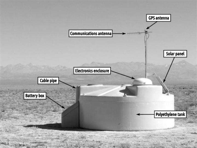
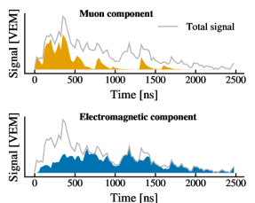
Figure 1: Left: A schematic view of a surface detector station in the field, showing its main components. Right: Signal in time measured by a single station of the SD for a simulated event. The total signal corresponds to the signal that can be measured by the SD. The signal from the electromagnetic and muon components are shown independently, as this information is available in simulations. The total signal is the sum of the muon component and the electromagnetic component. Our goal is to obtain the muon component using the total signal as an input.

This work focuses on the data collected with the SD, which operates with a duty cycle close to 100% and shows full detection efficiency for air showers above 3.16 EeV ($10^{18.5}$ eV). Charged particles traverse the 12 000 litres of ultra-pure water contained in each station of the SD and the emitted Cherenkov photons are collected by three nine-inch photomultiplier tubes (PMTs); see the left panel of Figure 1. The photomultiplier output is digitised at 40 MHz (25 ns bins) using 10 bit Flash Analog-Digital Converters (FADCs). Each signal trace has a length of 768 samples, corresponding to a time window of 19.2 $\upmu$s. The resulting signal is proportional to the sum of the Cherenkov radiation in water produced by electromagnetic particles (photons, electrons and positrons) and muons, see the right panel of Figure 1. Muons produce some characteristic features in the signal. As highly penetrating particles, they usually arrive at the stations at earlier times than the electromagnetic particles that undergo copious multiple scattering, see Fig. 4 in ref. [4]. The signal that muons produce is spiky, in contrast to the signal from electromagnetic particles, which is more continuous and spread in time. Since muons suffer less energy losses in the atmosphere than electromagnetic particles [5], they dominate the signals of the stations located far away from the core of the shower.

Based on the Heitler-Matthews extensive air-shower model and assuming the superposition principle [6], the number of muons $N_{\mu}^{A}$ in an extensive air shower produced by a nucleus with mass number $A$ can be related to the number of muons produced in a shower initiated by a proton with the same energy, $N_{\mu}^{\text{p}}$, through

$$N_{\mu}^{A}=N_{\mu}^{\text{p}}A^{1-\beta}.$$ (1.1)

where $1-\beta\simeq 0.1$. Therefore, the determination of the muon component in the air shower is crucial to infer, for each event, the mass of the primary particle, which is a key ingredient in the searches conducted to pinpoint the sources of UHECRs. Mass composition inferences are customarily carried out comparing observables measured in data and simulations.

With the current design of the SD, the separation of the muon and electromagnetic components can be done for events with large zenith angles [7] or for distances far off from the shower core [8]. Hence, for a majority of the recorded data, this separation cannot be performed in a straightforward and efficient way. In this work, starting from the total time trace, we estimate the muon signal for each individual WCD as a function of time using machine learning techniques. The applicability of the method is not restricted to a limited energy and/or zenith angle range but can be applied to the full data sample collected so far. However, for practical purposes, in this work we limit the discussion to the data set referred to as “vertical” events ($\theta<60^{\circ}$, where $\theta$ is the zenith angle) which are those for which it is harder to estimate the muon component with more straightforward techniques. As a novelty, we estimate the risetime [9] of the muon signal.

The branch of machine learning research studies algorithms and techniques that rely on inferring patterns from data. The scientist is only in charge of developing a suitable architecture, instead of designing every detail of a model. Numerous techniques were proposed many years ago but several recent breakthroughs in computational hardware have allowed for these techniques to be computationally affordable. Nowadays, machine learning is being used extensively in physics (for a recent review see e.g. ref. [10]). It is especially well suited for experiments in particle physics [11] and in astroparticle physics. The large amount of events collected by state-of-the-art experiments in both fields allows for the exploitation of machine learning techniques that require vast amounts of data to build and train a model.

An example of a previous work devoted to the extraction of the muon signal using machine learning can be found in ref. [12]. In this work, we focus our interest on the study of time series. Hence, from the large set of machine learning algorithms, we have chosen deep learning since it is the one that has lately experienced substantial progress when applied to temporal series and sequences. We go one step beyond to what is discussed in ref. [12], where only the integral of the muon trace was obtained. For the first time, we estimate the muon contribution to the signal recorded in each time bin.

This article is structured as follows. In Section 2, we give an overview of the methodology, the architecture of the neural network and the training method. In Section 3, we show the results of the neural network. We conclude by discussing the application of the neural network to data and assess its performance scrutinizing standard properties of extensive air showers.

2 The method

Our approach is based on Recurrent Neural Networks (RNNs). RNNs are specially well-suited for time series due to their memory mechanism. As the computing process develops, for each step of the temporal series, the RNN stores information from a preceding time slot that can be used at a later stage. Nowadays, RNNs are used successfully in different fields such as natural language processing or machine translation, see for example [13]. There are several kinds of RNNs and, among them, we have chosen one of the most common, known as Long Short Term Memory (LSTM) [14, 15].

2.1 The input

The traces recorded by the water-Cherenkov detectors of the SD are the input to the neural network. The electronics is used to sample the signals in bins of 25 ns. Once they are calibrated, the signals are expressed in Vertical Equivalent Muons (VEMs), which correspond to the most-likely signal deposited by a muon that traverses the center of the detector top-down. The traces used in this study are obtained after averaging the traces of every functioning PMT in a WCD.

We use only the first 200 bins (5 $\upmu$s) of each trace. Traces that are shorter than those 200 bins are padded with zeros at the end. This choice is made because the most relevant information is encapsulated in the first 200 bins of each trace, while choosing too many bins increases the computational time and memory needed to train the neural network. From simulations we know that for $E<10^{19}$ eV, around 90% of the stations have the complete muon signal in the first 200 bins and the remaining stations have more than 99% of the muon signal in those 200 bins. For $E>10^{19}$ eV, around 70% of the stations have the complete muon signal in the first 200 bins and the remaining stations have around 99% of the muon signal contained in those 200 bins. The fraction of the muon signal outside the first 200 bins is then negligible and can be ignored.

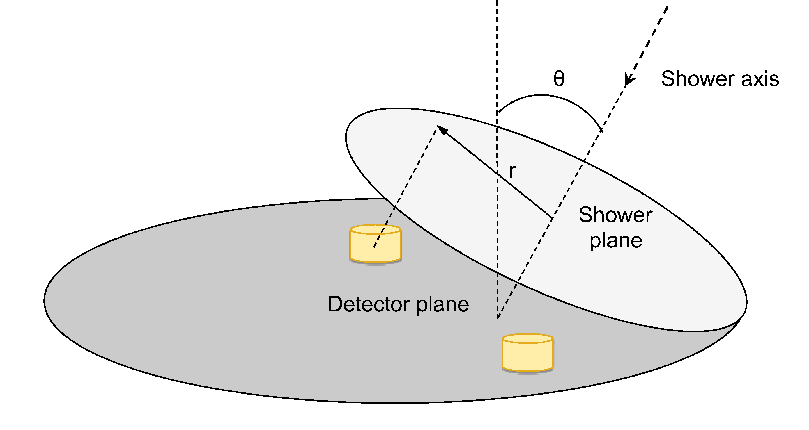
Figure 2: Schematic diagram of the geometry of an event, modified from ref. [16]. The angle $\theta$ is the angle between the shower axis and the zenith, the distance $r$ is the distance between the shower axis and the perpendicular projection of the station in the shower plane.

The trace information is not enough to accurately determine the muon component of extensive air showers. We found that the amount of atmosphere that the particles traverse plays an important role, since the electromagnetic and muon components are attenuated differently in the atmosphere. Particles from the electromagnetic component interact and scatter; the cascade continues down to energies below 1 MeV until electrons slow down through ionization without further radiating. In contrast, muons are very penetrating particles that traverse the atmosphere practically unaffected. This is why they also arrive earlier than electromagnetic particles. Muons are typically minimum ionizing particles. Consequently, as the attenuation of electrons, positrons and photons increases, the traces richer in muons become spikier and shorter in time.

This is the reason behind our choice of using as input two more variables: the secant of the reconstructed zenith angle, $\sec\theta$, and the distance to the core on the plane perpendicular to the shower (the shower plane), $r$, see Figure 2. $\theta$ is the reconstructed angle between the zenith and the trajectory of the primary cosmic ray. It results from a geometrical reconstruction carried out using the arrival time of particles at the stations and their respective locations [17]. From this reconstruction, the position of the core of the shower at the ground is estimated. Both variables take into account the amount of atmosphere crossed by particles. For $\theta\lesssim 80^{\circ}$, the amount of traversed atmosphere is proportional to $\sec\theta$ and as $r$ increases, the distance travelled by particles through the atmosphere gets larger.

Other variables, such as the energy of the primary cosmic ray, do not help to improve the performance of the neural network when they are included. By not including it, we also avoid the need to match the energy scale of data with that of simulations, which proves to be a difficult task. The application of this method to data is then straightforward since the zenith angle and distance to the core depend only on the geometrical reconstruction of the event.

2.2 Recurrent Neural Network (RNN) architecture

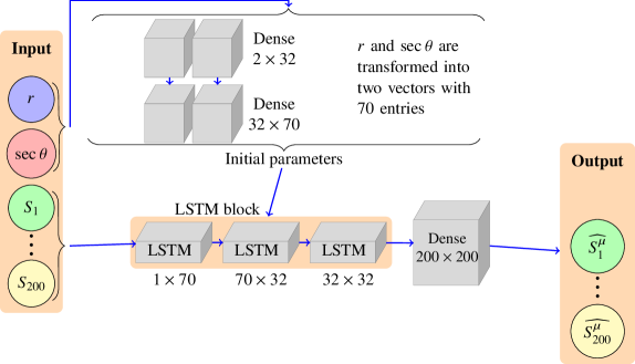
Figure 3: Schematic drawing of the input, architecture and output of the neural network. See the text for details.

The neural network architecture depicted in Figure 3 is set up as follows. The input is a vector of 202 components: distance to the core $r$, secant of the zenith angle $\sec\theta$ and the 200 values of each trace $S_{1},S_{2},\dots,S_{200}$, where $S_{i}$ is the value of the signal measured at the time bin $t_{i}$. At the start, this input is split into two sets. One of them is the set of the time-independent variables, i.e. $r$ and $\sec\theta$. These variables are fed into a set of fully-connected layers that will compute the initial hidden state and cell state for the first layer of LSTMs. The fully-connected layers transform the inital vector of two values ($r$, $\sec\theta$) into a vector of dimension 32 and then to a vector of dimension 70. The outputs of the fully-connected layers together with the 200 time values of each trace form the input to the LSTMs. Starting from a single sequence of 200 numbers (the signal $S_{i}$), the LSTMs produce 70, 32 and 32 sequences of 200 numbers, and the last one of these sequences is fed to a final fully-connected layer. The activation function used for the fully connected layer is $f(x)=\max(0,x)$ and $\tanh$ for the LSTM layers. The model has a total of 87 212 trainable or free parameters.

The set of fully-connected layers computes the vector of initial parameters that encodes information about the amount of atmosphere crossed by the particles, which in turn changes the shape of the traces. Without this block, there is insufficient information for the neural network to distinguish between traces with high or low fractions of muons and will be biased: for example, it will overestimate the muon component for nearly vertical showers and underestimate it for more inclined showers. The block of LSTMs is responsible for computing the traces and using the temporal information of the input.

2.3 Data selection and training

The neural network is trained with a library of simulated showers, with the same number of showers initiated by protons, helium, oxygen and iron nuclei. The energy range covered by simulations spans from $10^{18.5}$ eV to $10^{20.2}$ eV for zenith angles up to $60^{\circ}$. Each shower is simulated with the CORSIKA software [18] using the EPOS-LHC hadronic interaction model [19] and then reconstructed using the $\overline{\textrm{Off}}$ $\underline{\textrm{line}}$ software of the Pierre Auger Collaboration [20]. Among those simulated events, we select those that fulfill the quality condition that the station measuring the highest signal has to be surrounded by six operating neighbours, thus avoiding events that fall at the edges of the array. The method is applied to traces whose signals do not show any sign of saturation caused by an overflow of the read-out electronics or a loss of the linear behaviour of the PMT. Finally, only traces for which the integral is more than 5 VEM are included.

A total of around 450 000 events were available. The events were sampled randomly and assigned to the training, validation or test data sets using a uniform distribution in energy and $\sec\theta$ for the validation and test sets; the remaining events were assigned to the training set. The training data set does not require special care regarding the energy and zenith angle distributions since the dependence on the energy is mild and the zenith angle is given as input. The whole event sample was split as follows: around 390 000 in the training set, 22 000 in the validation set and 34 000 in the test set.

Before training, both $r$ and $\sec\theta$ values are scaled to be between 0 and 1 and all the traces are scaled individually to be between 0 and 1. The true (simulated) muon trace is scaled with the same factor used for the total trace. The output of the neural network is also between 0 and 1 so as to use the same factor to rescale back the predicted trace. The loss function that is minimized in the process of training is the mean squared error, defined for the trace of a single WCD as

$$L=\frac{1}{200}\sum_{i=1}^{200}\left(\widehat{S\rule{0.0pt}{7.0pt}^{\mu}}_{i}-{S\rule{0.0pt}{7.0pt}^{\mu}}_{i}\right)^{2}.$$ (2.1)

It corresponds to the average of the squares of the differences between the true muon trace ${S\rule{0.0pt}{7.0pt}^{\mu}}_{i}$ and the predicted muon trace $\widehat{S\rule{0.0pt}{7.0pt}^{\mu}}_{i}$, for each time bin $i$. The neural network is trained in batches and for each batch, the value of $L$ is computed for each trace and averaged over all the samples in the batch.

The training was done with the optimizer ADAM [21] with a fixed learning rate of $10^{-4}$ and the default values for the rest of the parameters; see ref. [21]. Using a batch size of 516 and 150 complete iterations over the whole training set or epochs on an Nvidia 2080 Ti GPU, the training takes around 8 hours. The loss as a function of the epoch is shown in Figure 4 for both the training and validation sets. We can see that the curve for the validation set decreases as the epoch increases. The curve for validation is below the one for training because, as explained before, a uniform distribution has been used for the validation data set and there are more events for which the performance is worse (lower zenith angles) in the training set. To further assess the goodness of our approach, the difference between the integral of the predicted and true muon traces is computed after each epoch. In the right panel of Figure 4, we show the mean and the standard deviation of the distribution of the difference. We use this measure because it has a straightforward physical interpretation. The mean controls the bias: i.e., if the mean is above zero, the neural network is consistently overestimating and vice versa. The standard deviation tells us how well we are predicting the muon signal, although this depends on many factors such as $\theta$, as we will see in Section 3. All the pipeline was implemented in Python 3.8 using Numpy [22] and Pandas [23] for the data treatment and Pytorch 1.5.0 [24] for the construction and training of the neural network.

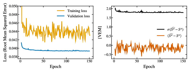
Figure 4: Left: Loss as a function of the epoch, see Eq. 2.1. Right: Mean value and standard deviation of the difference between the integral of the true muon signal and the predicted muon signal for the validation set.

Several tests were done to improve the performance of the method. Instead of predicting the average muon trace, we aimed at predicting the muon signal for each single PMT. These three independent results were averaged and compared to the main method (i.e., feeding the network with the average of the signals of the active PMTs). We found that even though the number of traces nearly tripled, the performance did not improve, with an increase of 0.2 VEM in the resolution or, in other words, around 1% with respect to the total signal (see the bottom right panel of Figure 7). We also tried other changes in the neural network such as increasing the number of layers or using a decaying learning rate, with no significant improvements in performance.

3 Results

We show examples of the predictions of the neural network in Figure 5. As a general comment, we observe that, qualitatively, the prediction follows the shape and peaks of the total signal. The network has learnt to reproduce the main features of the muon trace: its spiky shape and the fact that most muons arrive earlier. A thorough discussion of the results and their dependence on several variables are given in the next sections.

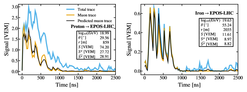
Figure 5: Examples of predicted muon traces for two simulated events with EPOS-LHC, for a electromagnetic-dominated signal (left) and muon-dominated signal (right). The prediction (black line) agrees well with the shape of the simulated muon trace (orange line) for a majority of the time bins. The blue thicker line corresponds to the total trace, the one measured by a WCD.

3.1 Integrals of the trace

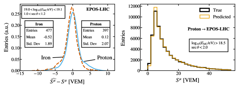
Figure 6: Left: Distribution of the difference between the integral of the predicted muon signal $\widehat{S^{\mu}}$ and the integral of the true muon signal $S^{\mu}$. Right: Distribution of $\widehat{S^{\mu}}$ and $S^{\mu}$ for all the stations in the test set.

One way to assess the performance of the method is to compute the integral of the predicted muon trace, $\widehat{S^{\mu}}=\sum_{i=1}^{200}\widehat{S\rule{0.0pt}{7.0pt}^{\mu}}_{i}$ and compare it to the integral of the true muon trace $S^{\mu}=\sum_{i=1}^{200}{S\rule{0.0pt}{7.0pt}^{\mu}}_{i}$. The integral of the muon trace is an interesting physical observable, since it relates to the total number of muons that reach the ground. In the left panel of Figure 6, we show a distribution with the difference between $\widehat{S^{\mu}}$ and $S^{\mu}$ for a particular bin of energy and zenith angle. The difference is compatible with zero and does not show a strong dependence with the value of the true muon signal. In the right panel of Figure 6, we show the distribution of $\widehat{S^{\mu}}$ and $S^{\mu}$ for all the WCDs in the test set for showers initiated by a proton primary. The two distributions have similar shapes.

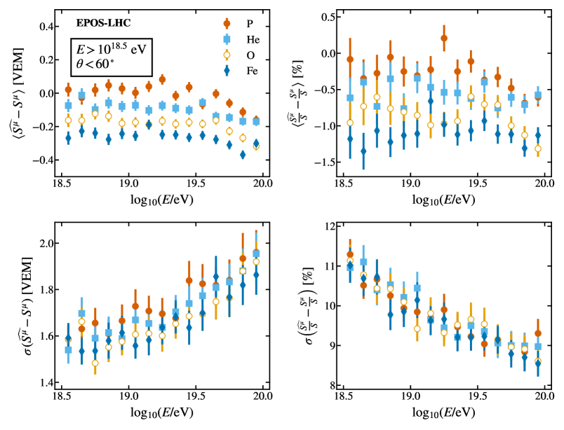
Figure 7: Left: Mean value (top) and standard deviation (bottom) of the difference between the predicted and values of the true muon signal as a function of energy. Right: Relative bias (top) and resolution (bottom) for the determination of the muon fraction as a function of the energy.

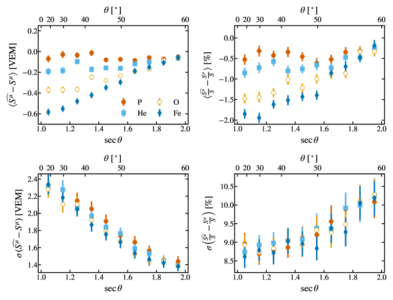
Figure 8: Left: Mean value (top) and standard deviation (bottom) of the difference between the predicted and values of the true muon signal as a function of $\sec\theta$. Right: Relative bias (top) and resolution (bottom) for the determination of the muon fraction as a function of the zenith angle.

In Figure 7 and Figure 8, the performances of the method are depicted as a function of the energy and $\sec\theta$, respectively. In the left panels, the mean value and standard deviation of the difference between the predicted and true values are shown for the different primaries. The mean values are close to zero and the standard deviation is less than 2 VEMs in most bins. These performances readily translate into the biases and resolutions for the muon fraction with respect to the total recorded signal shown in the right panels. The biases are within 2% for all the energies and angles explored here, regardless of the primaries. The resolutions are of the order of 11% at $10^{18.5}~{}$eV, improving with higher energies. The dependence on $\sec\theta$ reflects the attenuation of the overall signal at large zenith angles.

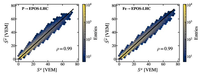
Figure 9: Integral of the predicted muon trace as a function of the integral of the true muon trace. The black line corresponds to a perfect prediction and $\rho$ is the Pearson correlation coefficient.

The performance of the method can be also evaluated as a function of the simulated muon signal ($S^{\mu}$). In Figure 9, we show the density plot of the predictions and the true values. The predictions are highly correlated with a Pearson correlation coefficient that is 0.99 for all the primaries. The mean and standard deviation of the distribution of $\widehat{S^{\mu}}-S^{\mu}$ are shown in Figure 10 as a function of $S^{\mu}$. The mean is close to zero and rarely exceeds 2 VEM. These results are observed to be zenith-angle dependent. The standard deviation increases as $S^{\mu}$ increases for more vertical events (left panel), while it remains constant at large angles (right panel) as a result of the preponderance of the muon signal.

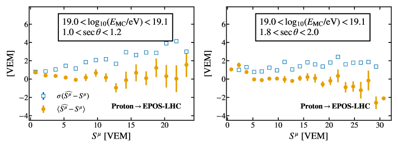
Figure 10: Mean and standard deviation of the difference between the integral of the predicted muon signal $\widehat{S^{\mu}}$ and the integral of the true muon signal $S^{\mu}$ for all the stations from events with the energies and zenith angles specified in the boxes.

For $S^{\mu}>5$ VEM, the resolution in the determination of the muon signal for each individual WCD goes from about 20% for the case of vertical events to 10% for events with $\sec\theta\simeq 2.0$

3.2 Risetime of the muon signal

The risetime of the recorded signals is another observable worth analysing, since it has been used successfully by the Pierre Auger Collaboration to extract valuable information about extensive air showers [16, 9]. The risetime $t_{1/2}$ is defined as the difference between two times, $t_{10}$ and $t_{50}$. $t_{10}$ is the time corresponding to the first time bin where the integral of the signal reaches 10 % of its total value, while $t_{50}$ is obtained when the integral reaches 50 % of the total. The risetime gives information about the shape of the trace: traces where the signal is concentrated in a few bins will have a shorter risetime, while traces where the signal is spread over time will have larger risetimes. In particular, the muon component has a smaller risetime than the electromagnetic component, since muons arrive earlier and in a shorter window of time [4].

In Figure 11, we compare the risetime of the predicted muon trace $\widehat{t\rule{0.0pt}{7.0pt}^{\mu}_{1/2}}$ with the risetime of the simulated muon trace $t\rule{0.0pt}{7.0pt}^{\mu}_{1/2}$. The standard deviation is less than 100 ns (4 time bins) for most values of the true risetime. This is a small time compared to the risetime of the total signal, which has a mean of 500 ns and 150 ns for the left and rights bins of Figure 11, respectively. Values with $t\rule{0.0pt}{7.0pt}^{\mu}_{1/2}<100$ ns correspond to around 1.5% of the samples in the left panel of Figure 11, since for vertical showers it is very rare to have the muon signal concentrated in very few bins, while for inclined showers it is rare that the muon signal is spread over a large time. The mean value approaches zero and the performance improves as the zenith angle increases. This means that the network successfully predicts not only the integral of the muon trace but also the shape of the muon trace.

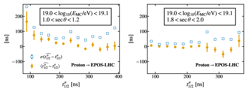
Figure 11: Mean and standard deviation of the difference between the risetime of the predicted muon signal $\widehat{t\rule{0.0pt}{7.0pt}^{\mu}_{1/2}}$ and the risetime of the true muon signal $t\rule{0.0pt}{7.0pt}^{\mu}_{1/2}$ for all the stations from events with the energies and zenith angles specified in the boxes.

3.3 Hadronic interaction model

We have chosen to train our neural network on simulations with the EPOS-LHC generator of hadronic interactions and presented some tests in the previous sections using the same event generator. We now test our method using simulations done with QGSJetII-04 [25] and Sibyll 2.3 [26] event generators. In other words, we test the predictions for simulations that are not only unknown to the neural network but that also have been generated using a different model of hadronic interactions.

QGSJetII-04.

In Figure 12, an example of a trace obtained with simulations produced using QGSJetII-04 is shown. The prediction follows the shape of the peaks, predicting quite accurately the muon signal. The difference between true and predicted muon signals does not show a strong deviance from zero.

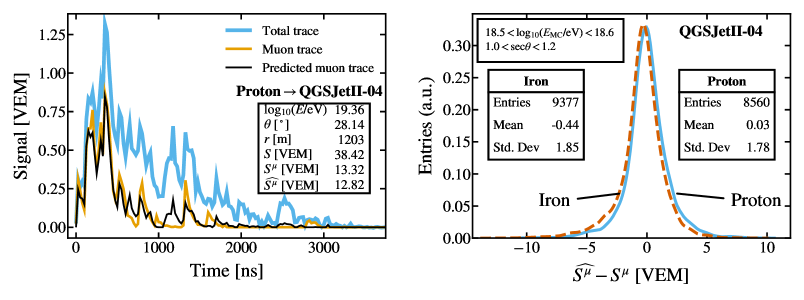
Figure 12: Left: Example of a predicted trace for a simulation of a proton generated air shower done with QGSJetII-04. Right: Distribution of $\widehat{S^{\mu}}-S^{\mu}$ for all the stations in the bin specified for simulations using proton and iron nuclei.

Sibyll 2.3.

In Figure 13, we show the result of predicting the muon traces for simulations performed with Sibyll 2.3. By comparing the values of the bias and of the resolution, we can see that the performance is similar to the case where the predictions were based on simulations done with QGSJetII-04.

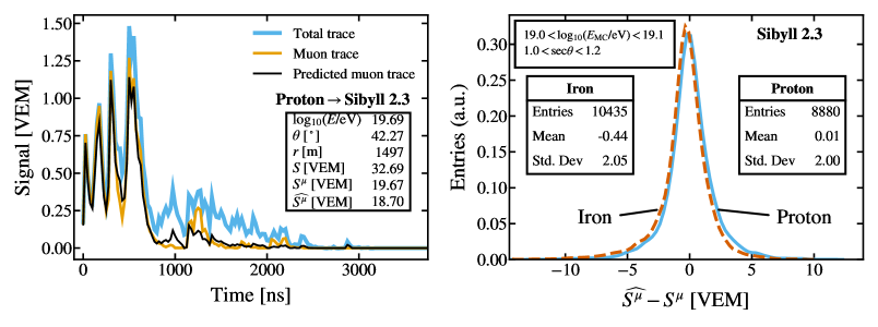
Figure 13: Left: Example of a predicted trace for a simulation done with Sibyll 2.3 with a proton as primary cosmic ray. Right: Distribution of $\widehat{S^{\mu}}-S^{\mu}$ for all the stations in the bin specified for simulations using proton and iron nuclei.

With these results we show that the neural network predictions rely essentially on the response of the detectors to muons and are thus independent of the hadronic interaction model used to simulate extensive air showers. For completeness, we have also carried out the opposite exercise: train the neural network with QGSJetII-04 and Sibyll 2.3 and predict for the other two models, respectively. The outcome is in a good agreement with the case where the neural network learns from events simulated with EPOS-LHC.

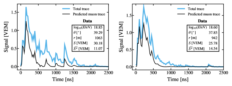
Figure 14: Examples of the predicted muon traces for two WCDs that belong to two different events recorded by the SD.

3.4 Comparison to data

In this section we assess how the neural network performs when applied to experimental data. The sample of events selected have the same cuts as the simulations used for training. In total, there are 177 000 events registered from 2004 to 2017. In Figure 14, we show examples of the muon trace predicted for two typical signals recorded with two independent WCDs. We observe that the output of the neural network produces features similar to those shown by the simulated traces of Figure 5, namely: the predicted muon signal is larger at earlier times since muons arrive earlier; in addition, the predicted muon trace exhibits a spiky structure.

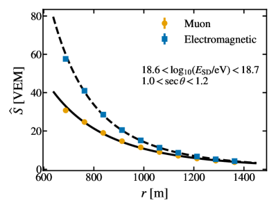
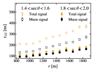
Figure 15: Left: Lateral distribution of the predicted muon and electromagnetic components for data. The solid and dashed lines are the outcome of two independent fits (see text for details). Right: Measured risetime of the total signal and risetime of the predicted muon signal as a function of the distance for two different zenith angle ranges.

A straightforward way to verify the robustness of the muon signal measurement is to study the behaviour of the total muon signal with the distance to the air-shower axis, i.e. the muon lateral distribution function (LDF). The muon LDF is illustrated in Figure 15, together with the electromagnetic one. For each WCD, we can obtain the electromagnetic component simply by subtracting the predicted muon signal from the total recorded signal. This endows us with the additional possibility to study the behaviour of the LDF of electromagnetic signals.

In addition, we compare our data to the parameterizations of the LDF of muon and electromagnetic particles that best fit the Akeno measurements. The authors of ref. [27] studied the properties of muons above 1 GeV at different distances to the shower core for events with $\sec\theta<1.2$. The behaviour of the Akeno data is well reproduced by the function proposed by Greisen in ref. [28], Eqs. (4) and (6) in ref. [27]. We fit our data with those expressions and the parameters that best reproduce Akeno data, just leaving the overall normalization free. The outcome of the fit is shown as a solid line in Figure 15 for the energy range $10^{18.6}$ eV to $10^{18.7}$ eV. The level of agreement between our measurements and the muon lateral distribution function extracted from Akeno data is remarkable.

In ref. [29], the Akeno data are used to extract a parameterization of the density of the electromagnetic signal as a function of the distance to the shower core (Eq. (2.1) in ref. [29]). We use that parameterization to fit our predicted electromagnetic signal, leaving the overall normalization free and the parameter referred to as $\eta$ in the original publication. $\eta$ is left as a free parameter since it is a function of the measured electromagnetic signal (see Eq. (2.2) in ref. [29]). As for the case of muons, the agreement with the Akeno parameterization of the electromagnetic signals is very good (dashed line in Figure 15).

The data sample was also used to carry out a cross-check involving the arrival times of the particles: we compared the behaviour with the distance to the core and with the zenith angle of the risetimes measured for the total signal and the predicted muon signal, see the right panel of Figure 15. As expected, the muon risetime is consistently smaller since muons arrive earlier. As the zenith angle increases, the fraction of the muon signal grows, thus the risetime of the total signal and the muon risetime become more similar. This behaviour is correctly reproduced by the predictions of the RNN.

4 Conclusions

We have shown that over a broad range of energies and zenith angles, a Recurrent Neural Network is a suitable tool to predict the muon signals that are part of the time traces measured with each individual WCD of the SD of the Pierre Auger Observatory. The neural network is trained on simulations, but the predictions are independent of the model used to simulate hadronic interactions. The muon signal for each WCD can be measured with a resolution that decreases from 20% to 10% as the zenith angle increases. Likewise, the muon fraction with respect to the total signal is estimated with biases that are within a 2% and a resolution that is lower than 11%.

When applied to data, the behaviour of the extracted muon and electromagnetic signals agrees well with relevant measurements found in the literature while other observables, such as the risetime, follow the behaviour dictated by basic physics principles.

The combination of this algorithm with the future data collected with the upgraded Observatory [30] will represent a major step forward since arguably, we will achieve an unprecedented resolution in our capability to make mass estimates on an event-by-event basis.

    $\bullet$    

The Pierre Auger Collaboration

A. Aab⁸⁰, P. Abreu⁷², M. Aglietta^52,50, J.M. Albury¹², I. Allekotte¹, A. Almela^8,11, J. Alvarez-Muñiz⁷⁹, R. Alves Batista⁸⁰, G.A. Anastasi^61,50, L. Anchordoqui⁸⁷, B. Andrada⁸, S. Andringa⁷², C. Aramo⁴⁸, P.R. Araújo Ferreira⁴⁰, J. C. Arteaga Velázquez⁶⁶, H. Asorey⁸, P. Assis⁷², G. Avila¹⁰, A.M. Badescu⁷⁵, A. Bakalova³⁰, A. Balaceanu⁷³, F. Barbato^43,44, R.J. Barreira Luz⁷², K.H. Becker³⁶, J.A. Bellido^12,68, C. Berat³⁴, M.E. Bertaina^61,50, X. Bertou¹, P.L. Biermann^b, T. Bister⁴⁰, J. Biteau³⁵, J. Blazek³⁰, C. Bleve³⁴, M. Boháčová³⁰, D. Boncioli^55,44, C. Bonifazi²⁴, L. Bonneau Arbeletche¹⁹, N. Borodai⁶⁹, A.M. Botti⁸, J. Brack^d, T. Bretz⁴⁰, P.G. Brichetto Orchera⁸, F.L. Briechle⁴⁰, P. Buchholz⁴², A. Bueno⁷⁸, S. Buitink¹⁴, M. Buscemi⁴⁵, K.S. Caballero-Mora⁶⁵, L. Caccianiga^57,47, F. Canfora^80,82, I. Caracas³⁶, J.M. Carceller⁷⁸, R. Caruso^56,45, A. Castellina^52,50, F. Catalani¹⁷, G. Cataldi⁴⁶, L. Cazon⁷², M. Cerda⁹, J.A. Chinellato²⁰, K. Choi¹³, J. Chudoba³⁰, L. Chytka³¹, R.W. Clay¹², A.C. Cobos Cerutti⁷, R. Colalillo^58,48, A. Coleman⁹³, M.R. Coluccia⁴⁶, R. Conceição⁷², A. Condorelli^43,44, G. Consolati^47,53, F. Contreras¹⁰, F. Convenga^54,46, D. Correia dos Santos²⁶, C.E. Covault⁸⁵, S. Dasso^5,3, K. Daumiller³⁹, B.R. Dawson¹², J.A. Day¹², R.M. de Almeida²⁶, J. de Jesús^8,39, S.J. de Jong^80,82, G. De Mauro^80,82, J.R.T. de Mello Neto^24,25, I. De Mitri^43,44, J. de Oliveira²⁶, D. de Oliveira Franco²⁰, F. de Palma^54,46, V. de Souza¹⁸, E. De Vito^54,46, M. del Río¹⁰, O. Deligny³², A. Di Matteo⁵⁰, C. Dobrigkeit²⁰, J.C. D’Olivo⁶⁷, R.C. dos Anjos²³, M.T. Dova⁴, J. Ebr³⁰, R. Engel^37,39, I. Epicoco^54,46, M. Erdmann⁴⁰, C.O. Escobar^a, A. Etchegoyen^8,11, H. Falcke^80,83,82, J. Farmer⁹², G. Farrar⁹⁰, A.C. Fauth²⁰, N. Fazzini^a, F. Feldbusch³⁸, F. Fenu^52,50, B. Fick⁸⁹, J.M. Figueira⁸, A. Filipčič^77,76, T. Fodran⁸⁰, M.M. Freire⁶, T. Fujii^92,e, A. Fuster^8,11, C. Galea⁸⁰, C. Galelli^57,47, B. García⁷, A.L. Garcia Vegas⁴⁰, H. Gemmeke³⁸, F. Gesualdi^8,39, A. Gherghel-Lascu⁷³, P.L. Ghia³², U. Giaccari⁸⁰, M. Giammarchi⁴⁷, M. Giller⁷⁰, J. Glombitza⁴⁰, F. Gobbi⁹, F. Gollan⁸, G. Golup¹, M. Gómez Berisso¹, P.F. Gómez Vitale¹⁰, J.P. Gongora¹⁰, J.M. González¹, N. González¹³, I. Goos^1,39, D. Góra⁶⁹, A. Gorgi^52,50, M. Gottowik³⁶, T.D. Grubb¹², F. Guarino^58,48, G.P. Guedes²¹, E. Guido^50,61, S. Hahn^39,8, P. Hamal³⁰, M.R. Hampel⁸, P. Hansen⁴, D. Harari¹, V.M. Harvey¹², A. Haungs³⁹, T. Hebbeker⁴⁰, D. Heck³⁹, G.C. Hill¹², C. Hojvat^a, J.R. Hörandel^80,82, P. Horvath³¹, M. Hrabovský³¹, T. Huege^39,14, J. Hulsman^8,39, A. Insolia^56,45, P.G. Isar⁷⁴, P. Janecek³⁰, J.A. Johnsen⁸⁶, J. Jurysek³⁰, A. Kääpä³⁶, K.H. Kampert³⁶, B. Keilhauer³⁹, J. Kemp⁴⁰, H.O. Klages³⁹, M. Kleifges³⁸, J. Kleinfeller⁹, M. Köpke³⁷, N. Kunka³⁸, B.L. Lago¹⁶, R.G. Lang¹⁸, N. Langner⁴⁰, M.A. Leigui de Oliveira²², V. Lenok³⁹, A. Letessier-Selvon³³, I. Lhenry-Yvon³², D. Lo Presti^56,45, L. Lopes⁷², R. López⁶², L. Lu⁹⁴, Q. Luce³⁷, A. Lucero⁸, J.P. Lundquist⁷⁶, A. Machado Payeras²⁰, G. Mancarella^54,46, D. Mandat³⁰, B.C. Manning¹², J. Manshanden⁴¹, P. Mantsch^a, S. Marafico³², A.G. Mariazzi⁴, I.C. Mariş¹³, G. Marsella^59,45, D. Martello^54,46, H. Martinez¹⁸, O. Martínez Bravo⁶², M. Mastrodicasa^55,44, H.J. Mathes³⁹, J. Matthews⁸⁸, G. Matthiae^60,49, E. Mayotte³⁶, P.O. Mazur^a, G. Medina-Tanco⁶⁷, D. Melo⁸, A. Menshikov³⁸, K.-D. Merenda⁸⁶, S. Michal³¹, M.I. Micheletti⁶, L. Miramonti^57,47, S. Mollerach¹, F. Montanet³⁴, C. Morello^52,50, M. Mostafá⁹¹, A.L. Müller⁸, M.A. Muller²⁰, K. Mulrey¹⁴, R. Mussa⁵⁰, M. Muzio⁹⁰, W.M. Namasaka³⁶, A. Nasr-Esfahani³⁶, L. Nellen⁶⁷, M. Niculescu-Oglinzanu⁷³, M. Niechciol⁴², D. Nitz⁸⁹, D. Nosek²⁹, V. Novotny²⁹, L. Nožka³¹, A Nucita^54,46, L.A. Núñez²⁸, M. Palatka³⁰, J. Pallotta², P. Papenbreer³⁶, G. Parente⁷⁹, A. Parra⁶², M. Pech³⁰, F. Pedreira⁷⁹, J. Pȩkala⁶⁹, R. Pelayo⁶⁴, J. Peña-Rodriguez²⁸, E.E. Pereira Martins^37,8, J. Perez Armand¹⁹, C. Pérez Bertolli^8,39, M. Perlin^8,39, L. Perrone^54,46, S. Petrera^43,44, T. Pierog³⁹, M. Pimenta⁷², V. Pirronello^56,45, M. Platino⁸, B. Pont⁸⁰, M. Pothast^82,80, P. Privitera⁹², M. Prouza³⁰, A. Puyleart⁸⁹, S. Querchfeld³⁶, J. Rautenberg³⁶, D. Ravignani⁸, M. Reininghaus^39,8, J. Ridky³⁰, F. Riehn⁷², M. Risse⁴², V. Rizi^55,44, W. Rodrigues de Carvalho¹⁹, J. Rodriguez Rojo¹⁰, M.J. Roncoroni⁸, M. Roth³⁹, E. Roulet¹, A.C. Rovero⁵, P. Ruehl⁴², S.J. Saffi¹², A. Saftoiu⁷³, F. Salamida^55,44, H. Salazar⁶², G. Salina⁴⁹, J.D. Sanabria Gomez²⁸, F. Sánchez⁸, E.M. Santos¹⁹, E. Santos³⁰, F. Sarazin⁸⁶, R. Sarmento⁷², C. Sarmiento-Cano⁸, R. Sato¹⁰, P. Savina^54,46,32, C.M. Schäfer³⁹, V. Scherini⁴⁶, H. Schieler³⁹, M. Schimassek^37,8, M. Schimp³⁶, F. Schlüter^39,8, D. Schmidt³⁷, O. Scholten^81,14, P. Schovánek³⁰, F.G. Schröder^93,39, S. Schröder³⁶, J. Schulte⁴⁰, S.J. Sciutto⁴, M. Scornavacche^8,39, A. Segreto^51,45, S. Sehgal³⁶, R.C. Shellard¹⁵, G. Sigl⁴¹, G. Silli^8,39, O. Sima^73,f, R. Šmída⁹², P. Sommers⁹¹, J.F. Soriano⁸⁷, J. Souchard³⁴, R. Squartini⁹, M. Stadelmaier^39,8, D. Stanca⁷³, S. Stanič⁷⁶, J. Stasielak⁶⁹, P. Stassi³⁴, A. Streich^37,8, M. Suárez-Durán²⁸, T. Sudholz¹², T. Suomijärvi³⁵, A.D. Supanitsky⁸, J. Šupík³¹, Z. Szadkowski⁷¹, A. Taboada³⁷, A. Tapia²⁷, C. Taricco^61,50, C. Timmermans^82,80, O. Tkachenko³⁹, P. Tobiska³⁰, C.J. Todero Peixoto¹⁷, B. Tomé⁷², A. Travaini⁹, P. Travnicek³⁰, C. Trimarelli^55,44, M. Trini⁷⁶, M. Tueros⁴, R. Ulrich³⁹, M. Unger³⁹, L. Vaclavek³¹, M. Vacula³¹, J.F. Valdés Galicia⁶⁷, L. Valore^58,48, E. Varela⁶², V. Varma K.C.^8,39, A. Vásquez-Ramírez²⁸, D. Veberič³⁹, C. Ventura²⁵, I.D. Vergara Quispe⁴, V. Verzi⁴⁹, J. Vicha³⁰, J. Vink⁸⁴, S. Vorobiov⁷⁶, H. Wahlberg⁴, C. Watanabe²⁴, A.A. Watson^c, M. Weber³⁸, A. Weindl³⁹, L. Wiencke⁸⁶, H. Wilczyński⁶⁹, T. Winchen¹⁴, M. Wirtz⁴⁰, D. Wittkowski³⁶, B. Wundheiler⁸, A. Yushkov³⁰, O. Zapparrata¹³, E. Zas⁷⁹, D. Zavrtanik^76,77, M. Zavrtanik^77,76, L. Zehrer⁷⁶, A. Zepeda⁶³

¹

Centro Atómico Bariloche and Instituto Balseiro (CNEA-UNCuyo-CONICET), San Carlos de Bariloche, Argentina

²

Centro de Investigaciones en Láseres y Aplicaciones, CITEDEF and CONICET, Villa Martelli, Argentina

³

Departamento de Física and Departamento de Ciencias de la Atmósfera y los Océanos, FCEyN, Universidad de Buenos Aires and CONICET, Buenos Aires, Argentina

⁴

IFLP, Universidad Nacional de La Plata and CONICET, La Plata, Argentina

⁵

Instituto de Astronomía y Física del Espacio (IAFE, CONICET-UBA), Buenos Aires, Argentina

⁶

Instituto de Física de Rosario (IFIR) – CONICET/U.N.R. and Facultad de Ciencias Bioquímicas y Farmacéuticas U.N.R., Rosario, Argentina

⁷

Instituto de Tecnologías en Detección y Astropartículas (CNEA, CONICET, UNSAM), and Universidad Tecnológica Nacional – Facultad Regional Mendoza (CONICET/CNEA), Mendoza, Argentina

⁸

Instituto de Tecnologías en Detección y Astropartículas (CNEA, CONICET, UNSAM), Buenos Aires, Argentina

⁹

Observatorio Pierre Auger, Malargüe, Argentina

¹⁰

Observatorio Pierre Auger and Comisión Nacional de Energía Atómica, Malargüe, Argentina

¹¹

Universidad Tecnológica Nacional – Facultad Regional Buenos Aires, Buenos Aires, Argentina

¹²

University of Adelaide, Adelaide, S.A., Australia

¹³

Université Libre de Bruxelles (ULB), Brussels, Belgium

¹⁴

Vrije Universiteit Brussels, Brussels, Belgium

¹⁵

Centro Brasileiro de Pesquisas Fisicas, Rio de Janeiro, RJ, Brazil

¹⁶

Centro Federal de Educação Tecnológica Celso Suckow da Fonseca, Nova Friburgo, Brazil

¹⁷

Universidade de São Paulo, Escola de Engenharia de Lorena, Lorena, SP, Brazil

¹⁸

Universidade de São Paulo, Instituto de Física de São Carlos, São Carlos, SP, Brazil

¹⁹

Universidade de São Paulo, Instituto de Física, São Paulo, SP, Brazil

²⁰

Universidade Estadual de Campinas, IFGW, Campinas, SP, Brazil

²¹

Universidade Estadual de Feira de Santana, Feira de Santana, Brazil

²²

Universidade Federal do ABC, Santo André, SP, Brazil

²³

Universidade Federal do Paraná, Setor Palotina, Palotina, Brazil

²⁴

Universidade Federal do Rio de Janeiro, Instituto de Física, Rio de Janeiro, RJ, Brazil

²⁵

Universidade Federal do Rio de Janeiro (UFRJ), Observatório do Valongo, Rio de Janeiro, RJ, Brazil

²⁶

Universidade Federal Fluminense, EEIMVR, Volta Redonda, RJ, Brazil

²⁷

Universidad de Medellín, Medellín, Colombia

²⁸

Universidad Industrial de Santander, Bucaramanga, Colombia

²⁹

Charles University, Faculty of Mathematics and Physics, Institute of Particle and Nuclear Physics, Prague, Czech Republic

³⁰

Institute of Physics of the Czech Academy of Sciences, Prague, Czech Republic

³¹

Palacky University, RCPTM, Olomouc, Czech Republic

³²

CNRS/IN2P3, IJCLab, Université Paris-Saclay, Orsay, France

³³

Laboratoire de Physique Nucléaire et de Hautes Energies (LPNHE), Sorbonne Université, Université de Paris, CNRS-IN2P3, Paris, France

³⁴

Univ. Grenoble Alpes, CNRS, Grenoble Institute of Engineering Univ. Grenoble Alpes, LPSC-IN2P3, 38000 Grenoble, France

³⁵

Université Paris-Saclay, CNRS/IN2P3, IJCLab, Orsay, France

³⁶

Bergische Universität Wuppertal, Department of Physics, Wuppertal, Germany

³⁷

Karlsruhe Institute of Technology (KIT), Institute for Experimental Particle Physics, Karlsruhe, Germany

³⁸

Karlsruhe Institute of Technology (KIT), Institut für Prozessdatenverarbeitung und Elektronik, Karlsruhe, Germany

³⁹

Karlsruhe Institute of Technology (KIT), Institute for Astroparticle Physics, Karlsruhe, Germany

⁴⁰

RWTH Aachen University, III. Physikalisches Institut A, Aachen, Germany

⁴¹

Universität Hamburg, II. Institut für Theoretische Physik, Hamburg, Germany

⁴²

Universität Siegen, Department Physik – Experimentelle Teilchenphysik, Siegen, Germany

⁴³

Gran Sasso Science Institute, L’Aquila, Italy

⁴⁴

INFN Laboratori Nazionali del Gran Sasso, Assergi (L’Aquila), Italy

⁴⁵

INFN, Sezione di Catania, Catania, Italy

⁴⁶

INFN, Sezione di Lecce, Lecce, Italy

⁴⁷

INFN, Sezione di Milano, Milano, Italy

⁴⁸

INFN, Sezione di Napoli, Napoli, Italy

⁴⁹

INFN, Sezione di Roma “Tor Vergata”, Roma, Italy

⁵⁰

INFN, Sezione di Torino, Torino, Italy

⁵¹

Istituto di Astrofisica Spaziale e Fisica Cosmica di Palermo (INAF), Palermo, Italy

⁵²

Osservatorio Astrofisico di Torino (INAF), Torino, Italy

⁵³

Politecnico di Milano, Dipartimento di Scienze e Tecnologie Aerospaziali , Milano, Italy

⁵⁴

Università del Salento, Dipartimento di Matematica e Fisica “E. De Giorgi”, Lecce, Italy

⁵⁵

Università dell’Aquila, Dipartimento di Scienze Fisiche e Chimiche, L’Aquila, Italy

⁵⁶

Università di Catania, Dipartimento di Fisica e Astronomia, Catania, Italy

⁵⁷

Università di Milano, Dipartimento di Fisica, Milano, Italy

⁵⁸

Università di Napoli “Federico II”, Dipartimento di Fisica “Ettore Pancini”, Napoli, Italy

⁵⁹

Università di Palermo, Dipartimento di Fisica e Chimica ”E. Segrè”, Palermo, Italy

⁶⁰

Università di Roma “Tor Vergata”, Dipartimento di Fisica, Roma, Italy

⁶¹

Università Torino, Dipartimento di Fisica, Torino, Italy

⁶²

Benemérita Universidad Autónoma de Puebla, Puebla, México

⁶³

Centro de Investigación y de Estudios Avanzados del IPN (CINVESTAV), México, D.F., México

⁶⁴

Unidad Profesional Interdisciplinaria en Ingeniería y Tecnologías Avanzadas del Instituto Politécnico Nacional (UPIITA-IPN), México, D.F., México

⁶⁵

Universidad Autónoma de Chiapas, Tuxtla Gutiérrez, Chiapas, México

⁶⁶

Universidad Michoacana de San Nicolás de Hidalgo, Morelia, Michoacán, México

⁶⁷

Universidad Nacional Autónoma de México, México, D.F., México

⁶⁸

Universidad Nacional de San Agustin de Arequipa, Facultad de Ciencias Naturales y Formales, Arequipa, Peru

⁶⁹

Institute of Nuclear Physics PAN, Krakow, Poland

⁷⁰

University of Łódź, Faculty of Astrophysics, Łódź, Poland

⁷¹

University of Łódź, Faculty of High-Energy Astrophysics,Łódź, Poland

⁷²

Laboratório de Instrumentação e Física Experimental de Partículas – LIP and Instituto Superior Técnico – IST, Universidade de Lisboa – UL, Lisboa, Portugal

⁷³

“Horia Hulubei” National Institute for Physics and Nuclear Engineering, Bucharest-Magurele, Romania

⁷⁴

Institute of Space Science, Bucharest-Magurele, Romania

⁷⁵

University Politehnica of Bucharest, Bucharest, Romania

⁷⁶

Center for Astrophysics and Cosmology (CAC), University of Nova Gorica, Nova Gorica, Slovenia

⁷⁷

Experimental Particle Physics Department, J. Stefan Institute, Ljubljana, Slovenia

⁷⁸

Universidad de Granada and C.A.F.P.E., Granada, Spain

⁷⁹

Instituto Galego de Física de Altas Enerxías (IGFAE), Universidade de Santiago de Compostela, Santiago de Compostela, Spain

⁸⁰

IMAPP, Radboud University Nijmegen, Nijmegen, The Netherlands

⁸¹

KVI – Center for Advanced Radiation Technology, University of Groningen, Groningen, The Netherlands

⁸²

Nationaal Instituut voor Kernfysica en Hoge Energie Fysica (NIKHEF), Science Park, Amsterdam, The Netherlands

⁸³

Stichting Astronomisch Onderzoek in Nederland (ASTRON), Dwingeloo, The Netherlands

⁸⁴

Universiteit van Amsterdam, Faculty of Science, Amsterdam, The Netherlands

⁸⁵

Case Western Reserve University, Cleveland, OH, USA

⁸⁶

Colorado School of Mines, Golden, CO, USA

⁸⁷

Department of Physics and Astronomy, Lehman College, City University of New York, Bronx, NY, USA

⁸⁸

Louisiana State University, Baton Rouge, LA, USA

⁸⁹

Michigan Technological University, Houghton, MI, USA

⁹⁰

New York University, New York, NY, USA

⁹¹

Pennsylvania State University, University Park, PA, USA

⁹²

University of Chicago, Enrico Fermi Institute, Chicago, IL, USA

⁹³

University of Delaware, Department of Physics and Astronomy, Bartol Research Institute, Newark, DE, USA

⁹⁴

University of Wisconsin-Madison, Department of Physics and WIPAC, Madison, WI, USA

—–

^a

Fermi National Accelerator Laboratory, Fermilab, Batavia, IL, USA

^b

Max-Planck-Institut für Radioastronomie, Bonn, Germany

^c

School of Physics and Astronomy, University of Leeds, Leeds, United Kingdom

^d

Colorado State University, Fort Collins, CO, USA

^e

now at Hakubi Center for Advanced Research and Graduate School of Science, Kyoto University, Kyoto, Japan

^f

also at University of Bucharest, Physics Department, Bucharest, Romania

References

- [1] Pierre Auger collaboration, Features of the energy spectrum of cosmic rays above eV using the Pierre Auger Observatory, Phys. Rev. Lett. 125 (2020) 121106 [2008.06488].
- [2] Pierre Auger collaboration, A measurement of the cosmic-ray energy spectrum above eV using the Pierre Auger Observatory, 2008.06486.
- [3] Pierre Auger collaboration, The Pierre Auger Cosmic Ray Observatory, Nucl. Instrum. Meth. A 798 (2015) 172 [1502.01323].
- [4] J. Linsley and L. Scarsi, Arrival Times of Air Shower Particles at Large Distances from the Axis, Physical Review 128 (1962) 2384.
- [5] T. K. Gaisser, R. Engel and E. Resconi, Cosmic Rays and Particle Physics: 2nd Edition. Cambridge University Press, 6, 2016.
- [6] J. Matthews, A Heitler model of extensive air showers, Astropart. Phys. 22 (2005) 387.
- [7] Pierre Auger collaboration, Muons in Air Showers at the Pierre Auger Observatory: Mean Number in Highly Inclined Events, Phys. Rev. D 91 (2015) 032003 [1408.1421].
- [8] Pierre Auger collaboration, Muons in Air Showers at the Pierre Auger Observatory: Measurement of Atmospheric Production Depth, Phys. Rev. D 90 (2014) 012012 [1407.5919].
- [9] Pierre Auger collaboration, Inferences on mass composition and tests of hadronic interactions from 0.3 to 100 EeV using the water-Cherenkov detectors of the Pierre Auger Observatory, Phys. Rev. D 96 (2017) 122003 [1710.07249].
- [10] G. Carleo, I. Cirac, K. Cranmer, L. Daudet, M. Schuld, N. Tishby et al., Machine learning and the physical sciences, Rev. Mod. Phys. 91 (2019) 045002 [1903.10563].
- [11] A Living Review of Machine Learning for Particle Physics, https://iml-wg.github.io/HEPML-LivingReview/.
- [12] A. Guillen, A. Bueno, J. Carceller, J. Martinez-Velazquez, G. Rubio, C. Todero Peixoto et al., Deep learning techniques applied to the physics of extensive air showers, Astropart. Phys. 111 (2019) 12 [1807.09024].
- [13] A. Karpathy, The Unreasonable Effectiveness of Recurrent Neural Networks, (2015), https://karpathy.github.io/2015/05/21/rnn-effectiveness/.
- [14] S. Hochreiter and J. Schmidhuber, Long Short-Term Memory, Neural Comput. 9 (1997) 1735.
- [15] C. Olah, Understanding LSTM Networks, (2015), https://colah.github.io/posts/2015-08-Understanding-LSTMs/.
- [16] Pierre Auger collaboration, Azimuthal Asymmetry in the Risetime of the Surface Detector Signals of the Pierre Auger Observatory, Phys. Rev. D 93 (2016) 072006 [1604.00978].
- [17] Pierre Auger collaboration, Reconstruction of Events Recorded with the Surface Detector of the Pierre Auger Observatory, Journal of Instrumentation 15 (2020) P10021 [2007.09035].
- [18] D. Heck, J. Knapp, J. Capdevielle, G. Schatz and T. Thouw, CORSIKA: A Monte Carlo code to simulate extensive air showers, .
- [19] T. Pierog, I. Karpenko, J. Katzy, E. Yatsenko and K. Werner, EPOS LHC: Test of collective hadronization with data measured at the CERN Large Hadron Collider, Phys. Rev. C 92 (2015) 034906 [1306.0121].
- [20] Pierre Auger collaboration, The offline software framework of the Pierre Auger Observatory, in 2005 IEEE Nuclear Science Symposium and Medical Imaging Conference, no. 2, pp. 1000–1003, 2005, DOI [astro-ph/0601016].
- [21] D. P. Kingma and J. Ba, Adam: A Method for Stochastic Optimization, 1412.6980.
- [22] C. R. Harris, K. J. Millman, S. J. van der Walt, R. Gommers, P. Virtanen, D. Cournapeau et al., Array programming with NumPy, Nature 585 (2020) 357–362.
- [23] Wes McKinney, Data Structures for Statistical Computing in Python, Proceedings of the 9th Python in Science Conference (2010) 56.
- [24] A. Paszke, S. Gross, F. Massa, A. Lerer, J. Bradbury, G. Chanan et al., Pytorch: An imperative style, high-performance deep learning library, in Advances in Neural Information Processing Systems 32, H. Wallach, H. Larochelle, A. Beygelzimer, F. d'Alché-Buc, E. Fox and R. Garnett, eds., pp. 8024–8035, Curran Associates, Inc., (2019), http://papers.neurips.cc/paper/9015-pytorch-an-imperative-style-high-performance-deep-learning-library.pdf.
- [25] S. Ostapchenko, Monte Carlo treatment of hadronic interactions in enhanced Pomeron scheme: I. QGSJET-II model, Phys. Rev. D 83 (2011) 014018 [1010.1869].
- [26] E.-J. Ahn, R. Engel, T. K. Gaisser, P. Lipari and T. Stanev, Cosmic ray interaction event generator SIBYLL 2.1, Phys. Rev. D 80 (2009) 094003 [0906.4113].
- [27] AGASA collaboration, Muons (>= 1-GeV) in large extensive air showers of energies between eV and eV observed at Akeno, J. Phys. G 21 (1995) 1101.
- [28] K. Greisen, Cosmic Ray showers, Annual Review of Nuclear Science 10 (1960) 63.
- [29] M. Nagano, M. Teshima, Y. Matsubara, H. Dai, T. Hara, N. Hayashida et al., Energy spectrum of primary cosmic rays above eV determined from the extensive air shower experiment at Akeno, J. Phys. G 18 (1992) 423.
- [30] Pierre Auger collaboration, The Pierre Auger Observatory Upgrade - Preliminary Design Report, 1604.03637.