Wireless Network Coding with Intelligent Reflecting Surfaces

Abstract

Conventional wireless techniques are becoming inadequate for beyond fifth-generation (5G) networks due to latency and bandwidth considerations. To improve the error performance and throughput of wireless communication systems, we propose physical layer network coding (PNC) in an intelligent reflecting surface (IRS)-assisted environment. We consider an IRS-aided butterfly network, where we propose an algorithm for obtaining the optimal IRS phases. Also, analytic expressions for the bit error rate (BER) are derived. The numerical results demonstrate that the proposed scheme significantly improves the BER performance. For instance, the BER at the relay in the presence of a $32$-element IRS is three orders of magnitudes less than that without an IRS.

I Introduction

Conventional wireless communication techniques are becoming inadequate for beyond 5G networks because they, in general, have excessive network latency and low spectral efficiency [1]. Network coding is a promising solution to increase the throughput of wireless networks [2, 3]. It relies on the ability of the relay (router) to perform more complex operations than just forwarding [4]. One kind of network coding is PNC, where the physical broadcast nature of wireless links, which generally causes deleterious interference, is exploited to increase the network throughput [5, 2, 3, 4, 6]. Yet, higher bandwidth is required to support PNC with higher data rates, which necessitates a move toward the millimeter wave (mm-Wave) band. However, mm-Wave communication suffers from high path loss and is susceptible to blockages. These limitations suggest future sustainable networks, where the propagation channel itself can be controlled.

In this regard, so-called IRSs have been demonstrated to overcome some of the issues associated with mm-Waves [7]. An IRS is a flat surface which comprises many small passive elements, each of which can independently introduce phase changes to the incident signals [8]. Thus, unlike traditional relays, it does not need a dedicated energy source or consume any transmit power. An IRS can be easily integrated into walls, ceilings, and building facades [9]. IRSs can enhance communication performance in terms of coverage, energy efficiency, electromagnetic radiation reduction, and wireless localization accuracy [10, 11, 12, 13, 14]. Also, IRSs can improve the BER performance of over-air-computation (OAC) techniques [15, 16, 17]. This is achieved by smartly tuning the IRS phase profile, thereby significantly boosting the received signal power. In a sense, PNC is a kind of OAC as it is based on the linear or nonlinear aggregation of signals by the wireless medium; yet it has remained unstudied in the presence of IRSs.

In this paper, we propose a PNC scheme in an IRS-assisted environment to enhance the error performance and throughput of wireless communication systems, especially in unfavorable channel conditions for mm-Wave communication. As a proof of concept, we focus on the butterfly network, usually adopted as the basic setting in the framework of network coding [5, 18]. In this setting, the relay computes network-coded packets directly from the received signal. To improve BER performance, we optimize the IRS profile. Although, the problem is non-convex, we propose an efficient optimization algorithm based in matrix lifting. Then, we derive the analytic BER of IRS-aided butterfly network to judge error performance. Numerical results verify the significant improvement of BER performance due to the proposed scheme.

For notation, the probability of an event and expectation of a random variable are denoted by $\mathbb{P}\{\cdot\}$ and $\mathbb{E}\left[\cdot\right]$, respectively. Capital bold letters, e.g., $\mathbf{X}$, and small bold letters, e.g., $\mathbf{x}$, denote matrices and vectors, respectively. The notation $\operatorname{diag}(\mathbf{x})$ represents a diagonal matrix with diagonal $\mathbf{x}$, while $\operatorname{tr}\left(\cdot\right)$ denotes the matrix trace. The transpose and Hermitian of vectors or matrices are denoted as $(\cdot)^{T}$ and $(\cdot)^{H}$. The $l^{th}$ row and column of a matrix $\mathbf{X}$ are denoted by $\mathbf{x}_{(l)}$ and $\mathbf{x}_{l}$, respectively. The real part of complex number $z$ is denoted by $\Re{\left(z\right)}$. The $\ell_{2}$-norm of a vector $\mathbf{x}$ is denoted by $\left|\left|\mathbf{x}\right|\right|$.

II System Model

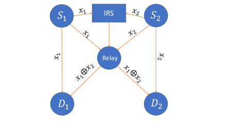
Figure 1: IRS-aided butterfly network.

This paper considers the IRS-aided butterfly network as shown in Fig. 1, where sources $\mathrm{S_{1}}$ and $\mathrm{S_{2}}$ want to deliver their messages to destinations $\mathrm{D_{1}}$ and $\mathrm{D_{2}}$. For simplicity, we assume each source and destination node have a single antenna to transmit and receive, respectively, whereas the relay node is equipped with ${N}_{\text{r}}=2$ antennas. To enhance communication performance from ${N}_{\textrm{s}}=2$ sources to relay, we propose deploying an IRS with $M$ reflecting elements, as in Fig. 1.

There are two stages in PNC. In the first stage, $\mathrm{S_{1}}$ and $\mathrm{S_{2}}$ broadcast their data to the relay and to destinations $\mathrm{D_{1}}$ and $\mathrm{D_{2}}$, respectively. Signals from $\mathrm{S_{1}}$ and $\mathrm{S_{2}}$ are assumed to arrive at the relay with symbol-level synchronization [3].

Let $P$ and $s_{i}$ be the transmit power and the transmitted symbol of source $i$, respectively. Hence, the signal transmitted by source $i$ is $x_{i}=\alpha_{i}s_{i}$, where $\alpha_{i}=\sqrt{P/\sigma_{s,i}^{2}}$. The power of $s_{i}$ is $\mathbb{E}\left[|s_{i}|^{2}\right]=\sigma_{s,i}^{2}$. We assume binary phase shift keying (BPSK) modulation at source nodes, but this also can be extended to quadrature phase shift keying (QPSK). The noise at the $j$th antenna of the relay is assumed to be complex Gaussian with $\mu$ mean and $\sigma^{2}$ variance, i.e., $n_{j}\sim\mathcal{CN}(\mu,\,\sigma^{2})$. We consider Rayleigh fading channels between IRS and relay, between sources and IRS, between sources and relay, between $\mathrm{S}_{1}$ and $\mathrm{D}_{1}$, and between relay and $\mathrm{D}_{1}$ as $\mathbf{H^{ir}}\in\mathbb{C}^{{N}_{\text{r}}\times M}$, $\mathbf{H^{ui}}\in\mathbb{C}^{M\times{N}_{\textrm{s}}}$, $\mathbf{H^{ur}}\in\mathbb{C}^{{N}_{\text{r}}\times{N}_{\textrm{s}}}$, $h_{\mathrm{D}_{1}}^{\mathrm{S}_{1}}\in\mathbb{C}^{1\times 1}$ and $\mathbf{h}_{\mathrm{D}_{1}}^{r}\in\mathbb{C}^{1\times{N}_{\text{r}}}$, respectively. The received signal at the relay node can be written in a matrix form as

$$\mathbf{r}=\left(\mathbf{H^{ir}}\mathbf{\Theta}\mathbf{H^{ui}}+\mathbf{H^{ur}}\right)\mathbf{x}+\mathbf{n}\triangleq\mathbf{H}\mathbf{x}+\mathbf{n},$$ (1)

where $\mathbf{\Theta}=\operatorname{diag}\left(\mathbf{v}\right)$ is the IRS diagonal phase shift matrix with $\mathbf{v}=\left[e^{j\theta_{1}},\ldots,e^{j\theta_{M}}\right]^{T}$ and $\theta_{m}\in\left[0,2\pi\right]$, $\mathbf{x}=\left[x_{1},x_{2}\right]^{T}$ and $\mathbf{n}=\left[n_{1},n_{2},\ldots,n_{{N}_{\text{r}}}\right]^{T}$ are the signal and noise vectors, respectively.

In the second stage, the relay computes an estimate of the XOR of the signals from $\mathrm{S_{1}}$ and $\mathrm{S_{2}}$. Here, the XORed version is referred to as the network-coded form. Then, the relay broadcasts the estimated network-coded signal to $\mathrm{D_{1}}$ and $\mathrm{D_{2}}$. The nodes $\mathrm{D_{1}}/\mathrm{D_{2}}$ can compute $x_{2}/x_{1}$ by XORing $x_{1}/x_{2}$ and a network-coded signal from the relay.

In naive network-layer network coding (NNC) rather than PNC, the relay computes the estimates of $x_{1}$ and $x_{2}$ before creating a network-coded form $x_{\tiny{\oplus}}\triangleq x_{1}\oplus x_{2}$. However, such schemes are suboptimal since they do not consider that only $x_{\tiny{\oplus}}$ is needed at the relay rather than individual signals $x_{1}$ and $x_{2}$ [3, 5].

Therefore, we propose PNC approach where the relay computes an estimate of $x_{\tiny{\oplus}}$ without decoding $x_{1}$ and $x_{2}$ individually. In fact, it is more useful to get the estimate of $x_{\tiny{\oplus}}$ from $x_{1}+x_{2}$ and $x_{1}-x_{2}$, which can be calculated directly from $\mathbf{r}$ via matrix multiplication. Hence, the relay can get $x_{\tiny{\oplus}}$ almost at full rate [19, 5].

Based on this observation, the received signal in (1) can be rewritten as

$$\mathbf{r}=\left(\mathbf{H}\mathbf{D}^{-1}\right)(\mathbf{D}\mathbf{x})+\mathbf{n}=\mathbf{\widetilde{H}}\widetilde{\mathbf{x}}+\mathbf{n}\mbox{,}$$ (2)

where

$$\mathbf{D}=2\mathbf{D}^{-1}=\left[\begin{array}[]{cc}1&1\\ 1&-1\end{array}\right]$$ (3)

is the sum-difference matrix, and $\widetilde{\mathbf{x}}$ is

$$\widetilde{\mathbf{x}}=\left[\begin{array}[]{c}\widetilde{x}_{1}\\ \widetilde{x}_{2}\end{array}\right]\triangleq\mathbf{D}\,\mathbf{x}=\left[\begin{array}[]{c}x_{1}+x_{2}\\ x_{1}-x_{2}\end{array}\right]\mbox{.}$$ (4)

The vector $\widetilde{\mathbf{x}}$ can be estimated from $\mathbf{r}$ using a linear operator as

$$\mathbf{y}=\mathbf{G}\mathbf{r}\mbox{,}$$ (5)

where $\mathbf{G}\in\mathbb{C}^{{N}_{\textrm{s}}\times{N}_{\text{r}}}$ is the beamforming matrix at the relay, designed in Section IV. We consider that the relay can estimate the channel state information (CSI).

III Problem Formulation

In this section, we aim to design the optimal linear operator, i.e., the beamforming matrix $\mathbf{G}$ and the IRS phase profile $\mathbf{\Theta}$ to minimize the mean-squared error (MSE) for the recovery of $\widetilde{\mathbf{x}}$. In this regard, the problem can be formulated as

$$\underset{\boldsymbol{\Theta},{\mathbf{G}}}{\operatorname{minimize}}\quad \mathsf{MSE}\triangleq\mathbb{E}\left[\|\mathbf{y}(\boldsymbol{\Theta},{\mathbf{G}})-\widetilde{\mathbf{x}}\|^{2}\right]$$ (6a)

subject to $$0\leq\theta_{m}\leq 2\pi,\ m\in{\{1,2,\ldots,M\}}.$$ (6b)

The MSE between the estimate $\mathbf{y}$ and target parameter $\widetilde{\mathbf{x}}$ can be computed as

$$\mathsf{MSE} =\operatorname{tr}\left(\mathbb{E}\{\left(\mathbf{G}\mathbf{r}-\widetilde{\mathbf{x}}\right)\left(\mathbf{r}^{H}\mathbf{G}^{H}-\widetilde{\mathbf{x}}^{H}\right)\}\right)$$

$$=\operatorname{tr}\left(\mathbf{G}\mathbb{E}\{\mathbf{r}\mathbf{r}^{H}\}\mathbf{G}^{H}-2\Re\{\mathbf{G}\mathbb{E}\{\mathbf{r}\widetilde{\mathbf{x}}^{H}\}\}+\mathbb{E}\{\widetilde{\mathbf{x}}\widetilde{\mathbf{x}}^{H}\}\right)$$

$$=\operatorname{tr}\left(\mathbf{G}(P\mathbf{H}\mathbf{H}^{H}+\sigma^{2}\mathbf{I})\mathbf{G}^{H}-2\Re\{\mathbf{G}P\mathbf{H}\mathbf{D}^{H}\}+2P\mathbf{I}\right)\mbox{.}$$ (7)

The joint optimization over the beamforming matrix and IRS profile in (6) is challenging. In Section IV, we provide an efficient algorithm for the optimization problem.

IV Optimization Algorithm

We propose an algorithm that optimizes the IRS phases while fixing the beamforming matrix in (6). In particular, for a fixed $\mathbf{\Theta}$ in (6), the optimization problem is a quadratic unconstrained problem in $\mathbf{G}$ that can be solved in a closed-form as

$$\mathbf{G}=(P\mathbf{H}^{H}\mathbf{H}+\sigma^{2}\mathbf{I})^{-1}P\mathbf{H}^{H}\mbox{,}$$ (8)

which is the minimum mean square error (MMSE) estimator for $\mathbf{G}$. To optimize the phases of IRS for fixed $\mathbf{G}$, we propose the matrix lifting technique [20]. First, the objective function should be written in terms of $\mathbf{v}$, i.e., $\mathsf{MSE}$ can be written as

$$\mathsf{MSE}\triangleq P\sum_{i^{\prime}=1}^{{N}_{\textrm{s}}}\sum_{j{\prime}=1}^{{N}_{\text{r}}}\left(\sum_{j=1}^{{N}_{\text{r}}}\mathbf{g}_{j}^{H}\mathbf{g}_{j^{\prime}}\left(b^{ji^{\prime}}\right)^{H}\right)b^{j^{\prime}i^{\prime}}+2P{N}_{\textrm{s}}\\ -2\,P\,\Re\left(\sum_{i=1}^{{N}_{\textrm{s}}}\sum_{j=1}^{{N}_{\text{r}}}b^{ji}\left(g_{1j}+(-1)^{i+1}g_{2j}\right)\right)+\sum_{i=1}^{{N}_{\textrm{s}}}{{\sigma}_{i}}^{2}\mbox{,}$$ (9)

where $b^{ji}=\boldsymbol{\phi}^{ji}\mathbf{v}+h_{ji}^{ur}$ and $\boldsymbol{\phi}^{ji}=\mathbf{h}^{\mathbf{ir}}_{(j)}\operatorname{diag}(\mathbf{h}^{\mathbf{ui}}_{i})$.

By substituting (8) in (9), we can write the optimization problem (6) for a fixed $\mathbf{G}$ as

$$\underset{\mathbf{v}}{\operatorname{minimize}}\quad \mathsf{MSE}$$ (10a)

subject to $$|\mathbf{v}(m)|^{2}=1,\ m\in\{1,2,\ldots,M\}\mbox{.}$$ (10b)

The unit modulus constraint induces non-convexity. In this regard, we apply a matrix lifting technique [20]. Now, the problem is tackled with the help of matrix $\mathbf{V}$, where

$$\mathbf{V}=\left[\begin{array}[]{c}\mathbf{v}\\ 1\end{array}\right]\left[\begin{array}[]{cc}\mathbf{v}^{H}&1\end{array}\right]=\left[\begin{array}[]{cc}\mathbf{v}\mathbf{v}^{H}&\mathbf{v}\\ \mathbf{v}^{H}&1\end{array}\right]\mbox{.}$$ (16)

For $\mathbf{V}$, we have the following constraints: $\operatorname{rank}\left(\mathbf{V}\right)\leq 1$, ${\mathbf{V}\geq 0}$, and $\mathbf{V}(k,k)=1$, $\forall k\in\{1,\ldots,M+1\}$. Let us rewrite (9) in terms of $\mathbf{V}$ and remove all the terms that do not depend on $\mathbf{v}$ as

$$\mathsf{MSE} \propto\!\!\sum_{i^{\prime}=1}^{{N}_{\textrm{s}}}\sum_{j{\prime}=1}^{{N}_{\text{r}}}\sum_{j=1}^{{N}_{\text{r}}}\!\!\operatorname{tr}\left(\mathbf{g}^{H}_{j}\mathbf{g}_{j^{\prime}}\!\!\left[\begin{array}[]{cc}{\boldsymbol{\phi}^{ji^{\prime}}}^{H}\boldsymbol{\phi}^{j^{\prime}i^{\prime}}&{\boldsymbol{\phi}^{ji^{\prime}}}^{H}h_{j^{\prime}i^{\prime}}^{ur}\\ h_{ji^{\prime}}^{*ur}\boldsymbol{\phi}^{j^{\prime}i^{\prime}}&0\end{array}\right]\mathbf{V}\right)$$ (19)

$$\phantom{\propto}-\sum_{i=1}^{{N}_{\textrm{s}}}\sum_{j=1}^{{N}_{\text{r}}}\operatorname{tr}\left(\left[\begin{array}[]{cc}0&\left(g_{1j}^{*}+(-1)^{i+1}g_{2j}^{*}\right){\boldsymbol{\phi}^{ji}}^{H}\\ 0&0\end{array}\right]\mathbf{V}\right)$$ (22)

$$\phantom{\propto}-\sum_{i=1}^{{N}_{\textrm{s}}}\sum_{j=1}^{{N}_{\text{r}}}\operatorname{tr}\left(\left[\begin{array}[]{cc}0&0\\ \left(g_{1j}+(-1)^{i+1}g_{2j}\right)\boldsymbol{\phi}^{ji}&0\end{array}\right]\mathbf{V}\right)$$ (25)

$$=\operatorname{tr}\left(\mathbf{A}\mathbf{V}\right)\mbox{,}$$ (26)

where $\mathbf{A}$ is a matrix representing the summation of all the matrices inside the trace function in (19). So, we have the following optimization problem

Algorithm 1 Algorithm of Optimizing $\mathbf{V}$ for Fixed $\mathbf{G}$

1:  Initialize $\mathbf{V}_{\mathrm{iter}}$ as in (16) with an arbitrary vector $\mathbf{v}$ that satisfies (10b) and set $\mathrm{iter}=1$

2:  repeat

3:     Step 1: Set $\mathbf{V}^{\prime}:=\mathbf{V}_{\mathrm{iter}}$

4:     Step 2: Solve convex problem (31), whose output is $\mathbf{V}$.

5:     Step 3: Update $\mathbf{V}_{\mathrm{iter}}:=\mathbf{V}$

6:     Step 4: Set $\mathrm{iter}=\mathrm{iter}+1$

7:  until $\left||\mathbf{V}_{\mathrm{iter}}-\mathbf{V}^{\prime}\right||^{2}_{F}\leq\delta$ or $\mathrm{iter}>\mathrm{Iter}_{\max}$

8:  $\mathbf{V}:=\mathbf{V}_{\mathrm{iter}}$

9:  Output $\mathbf{V}$

$$\underset{\mathbf{V}\geq 0}{\operatorname{minimize}}\quad \operatorname{tr}\left(\mathbf{A}\mathbf{V}\right)$$ (27a)

subject to $$\mathbf{V}(k,k)=1,\ k\in\{1,2,\ldots,M+1\}$$ (27b)

$$\operatorname{rank}\left(\mathbf{V}\right)\leq 1\mbox{.}$$ (27c)

The constraint $\operatorname{rank}\left(\mathbf{V}\right)\leq 1$ is non-convex and equivalent to

$$\operatorname{tr}\left(\mathbf{V}\right)-\beta_{1}\left(\mathbf{V}\right)=0,$$ (28)

where $\beta_{1}\left(\mathbf{V}\right)$ is the largest singular value of the matrix $\mathbf{V}$. Also, for $\mathbf{V}\geq 0$, i.e., semidefinite, the left side of (28) is $0$ when $\operatorname{rank}\left(\mathbf{V}\right)\leq 1$ is satisfied; otherwise, it is greater than zero. The optimization problem can be written as

$$\underset{\mathbf{V}\geq 0}{\operatorname{minimize}}\quad \left(\operatorname{tr}\left(\mathbf{A}\mathbf{V}\right)+\gamma\left(\operatorname{tr}\left(\mathbf{V}\right)-\beta_{1}\left(\mathbf{V}\right)\right)\right)$$ (29a)

subject to $$\mathbf{V}(k,k)=1,\ k\in\{1,2,\ldots,M+1\}\mbox{,}$$ (29b)

where $\gamma\geq 0$ is a fixed weight. Since $\beta_{1}\left(\mathbf{V}\right)$ and $\operatorname{tr}\left(\mathbf{A}\mathbf{V}\right)+\gamma\,\operatorname{tr}\left(\mathbf{V}\right)$ are convex functions in $\mathbf{V}$, (29) can be represented as a difference-of-convex functions (DC) problem. CCP can efficiently obtain a local optimal solution for DC problems [21]. In this regard, we linearize $-\gamma\,\beta_{1}(\mathbf{V})$, which induces non-convexity in (29), around a point $\mathbf{V}=\mathbf{V}^{\prime}$ using the following upper bound [16]

$$-\gamma\,\beta_{1}\left(\mathbf{V}\right)\leq-\gamma\,\operatorname{tr}\left(\mathbf{V}\mathbf{u_{1}}\left(\mathbf{V}^{\prime}\right)\mathbf{u_{1}}\left(\mathbf{V}^{\prime}\right)^{H}\right)\mbox{,}$$ (30)

where $\mathbf{u_{1}}\left(\mathbf{V}^{\prime}\right)$ is the eigenvector of the matrix $\mathbf{V}^{\prime}$ corresponding to its largest eigenvalue. The equality condition in (30) is satisfied when $\mathbf{V}=\mathbf{V}^{\prime}$. We get the following convex optimization problem, which can be solved by cvx:

$$\underset{\mathbf{V}\geq 0}{\operatorname{min}}\quad \operatorname{tr}\left(\mathbf{A}\mathbf{V}\right)+\gamma\left(\operatorname{tr}\left(\mathbf{V}\right)-\operatorname{tr}\left(\mathbf{V}\mathbf{u_{1}}\left(\mathbf{V}^{\prime}\right)\mathbf{u_{1}}\left(\mathbf{V}^{\prime}\right)^{H}\right)\right)$$ (31a)

s.t. $$\mathbf{V}(k,k)=1,\ k\in\{1,2,\ldots,M+1\}\mbox{.}$$ (31b)

Appropriate choice of the penalty parameter $\gamma$ in (31) can be found via simple bisection and remains static throughout Alg. 1. An iterative algorithm that alternately optimizes the phases of IRS and beamforming matrix $\mathbf{G}$ is given in Alg. 2.

Algorithm 2 Iterative Algorithm for MMSE Optimization

1:  Initialize $\mathbf{v}^{1}$ as an arbitrary vector that satisfies (10b) and set $k=0$

2:  repeat

3:     Step 1: Set $k=k+1$

4:     Step 2: Update $\mathbf{G}^{k}$ using (8), where diagonal elements of phase matrix $\mathbf{\Theta}$ are the elements of vector $\mathbf{v}^{k}$

5:     Step 3: Run Alg. 1, where $\mathbf{G}=\mathbf{G}^{k}$, and update $\mathbf{v}^{k+1}$ with the first $M$ elements in $\mathbf{v}_{M+1}$

6:  until $\left||\mathbf{v}_{k+1}-\mathbf{v}^{k}\right||^{2}+\left||\mathbf{G}_{k+1}-\mathbf{G}^{k}\right||^{2}_{F}<\delta$

V Optimal Detector and Error Performance

V-A Optimal Detector

The likelihood estimator can be considered to estimate the network coding form, i.e., $x_{\tiny{\oplus}}$, from $\mathbf{y}$. In this regard, the log likelihood ratio (LLR) can be written, ignoring the noise dependencies in $y_{1}$ and $y_{2}$, as

$$\mathcal{L}\left(x_{\tiny{\oplus}}|y_{1}y_{2}\right)=\log\left(\frac{\mathbb{P}\{y_{1}y_{2}|x_{\tiny{\oplus}}=1\}}{\mathbb{P}\{y_{1}y_{2}|x_{\tiny{\oplus}}=-1\}}\right)$$

$$=\log\left(\frac{\mathbb{P}\{y_{1}|\widetilde{x}_{1}=0\}\left[\mathbb{P}\{y_{2}|\widetilde{x}_{2}=2\}+\mathbb{P}\{y_{2}|\widetilde{x}_{2}=-2\}\right]}{\left[\mathbb{P}\{y_{1}|\widetilde{x}_{1}=2\}+\mathbb{P}\{y_{1}|\widetilde{x}_{1}=-2\}\right]\mathbb{P}\{y_{2}|\widetilde{x}_{2}=0\}}\right)$$

$$=2\left({\frac{1}{\sigma_{1}^{2}}-\frac{1}{\sigma_{2}^{2}}}\right)+\log\left(\frac{\cosh\left(2y_{2}/\sigma_{2}^{2}\right)}{\cosh\left(2y_{1}/\sigma_{1}^{2}\right)}\right)\mbox{,}$$ (32)

where $\sigma^{2}_{i}\triangleq\{\mathbf{G}\mathbf{G}^{H}\}_{i,i}\sigma^{2}$ is the noise variance on the $i$th stream after the linear operator. Let us first define the estimation of $x_{\tiny{\oplus}}$ at the relay and $\mathrm{D_{1}}$ as $\widehat{x}_{\tiny{\oplus}\mbox{,}\mathrm{r}}$ and $\widehat{x}_{\tiny{\oplus}\mbox{,}\mathrm{D}_{1}}$, respectively. The corresponding decision rules are then

$$\widehat{x}_{\tiny{\oplus}\mbox{,}\mathrm{r}} =\begin{cases}1&\text{ when }\mathcal{L}\left(x_{\tiny{\oplus}}|y_{1}y_{2}\right)\geq 0\\ -1&\text{ when }\mathcal{L}\left(x_{\tiny{\oplus}}|y_{1}y_{2}\right)<0\end{cases}\mbox{,}$$ (33)

$$\widehat{x}_{\tiny{\oplus}\mbox{,}\mathrm{D}_{1}} =\begin{cases}1&\text{ when }\mathcal{L}_{\mathrm{D}_{1}}^{r}\left(\widehat{x}_{\tiny{\oplus}\mbox{,}\mathrm{r}}|y_{\mathrm{D}_{1}}^{r}\right)\geq 0\\ -1&\text{ when }\mathcal{L}_{\mathrm{D}_{1}}^{r}\left(\widehat{x}_{\tiny{\oplus}\mbox{,}\mathrm{r}}|y_{\mathrm{D}_{1}}^{r}\right)<0\end{cases}\mbox{,}$$ (34)

where $\mathcal{L}_{\mathrm{D}_{1}}^{r}=2y_{\mathrm{D}_{1}}^{r}/\sigma_{r,\mathrm{D}_{1}}^{2}$ is the likelihood detector, and $y_{\mathrm{D}_{1}}^{r}$ is the received signal at $\mathrm{D}_{1}$ from relay. After the channel inversion, the variance of the noise at $\mathrm{D}_{1}$ is $\sigma_{r,\mathrm{D}_{1}}^{2}=\sigma^{2}/\lVert\mathbf{h}_{\mathrm{D}_{1}}^{r}\rVert^{2}$. After that, the relay broadcasts $\widehat{x}_{\tiny{\oplus}\mbox{,}\mathrm{r}}$ to the destinations. $\mathrm{D_{1}}$ receives $\widehat{x}_{\tiny{\oplus}\mbox{,}\mathrm{D}_{1}}$ and $\widehat{x}_{1}$, which is estimated similarly to $\widehat{x}_{\tiny{\oplus}\mbox{,}\mathrm{D}_{1}}$ with likelihood detector $\mathcal{L}_{\mathrm{D}_{1}}^{\mathrm{S}_{1}}=2y_{\mathrm{D}_{1}}^{\mathrm{S}_{1}}/\sigma_{\mathrm{S}_{1},\mathrm{D}_{1}}^{2}$, received signal $y_{\mathrm{D}_{1}}^{\mathrm{S}_{1}}$, and noise variance after channel inversion $\sigma_{\mathrm{S}_{1},\mathrm{D}_{1}}^{2}=\sigma^{2}/\lvert h_{\mathrm{D}_{1}}^{\mathrm{S}_{1}}\rvert^{2}$. Then, $\widehat{x}_{2}$ is obtained at $\mathrm{D}_{1}$ by XORing $\widehat{x}_{\tiny{\oplus}\mbox{,}\mathrm{D}_{1}}$ and $\widehat{x}_{1}$. Similarly, $\mathrm{D_{2}}$ receives $\widehat{x}_{2}$ and $\widehat{x}_{\tiny{\oplus}\mbox{,}\mathrm{D}_{2}}$, and obtains $\widehat{x}_{1}$ by XORing the two values.

V-B BER Analysis

Before calculating instantaneous theoretical BER at $\mathrm{D}_{1}$, i.e., $\mathbb{P}_{\mathrm{D}_{1}}\triangleq\mathbb{P}\left(\widehat{x}_{2}\neq x_{2}\right)$, we can find the instantaneous BERs separately for the links from sources to relay, from $\mathrm{S}_{1}$ to $\mathrm{D}_{1}$, and from relay to $\mathrm{D_{1}}$. Let us define the set $\mathbb{X}\triangleq\{-2,2\}$, which contains all the values of $\widetilde{x}_{2}$ and $\widetilde{x}_{1}$ such that $x_{\tiny{\oplus}}=1$ and $x_{\tiny{\oplus}}=-1$, respectively. To obtain $\widetilde{\mathbf{x}}$ at the relay from $y_{1}$ and $y_{2}$, we use the LLR in (V-A). To derive $\mathbb{P}^{\mathrm{r}}_{\tiny{\oplus}}\triangleq\mathbb{P}\left(\widehat{x}_{\tiny{\oplus}\mbox{,}\mathrm{r}}\neq x_{\tiny{\oplus}}\right)$ at the relay, we need to further rewrite (V-A) as

$$\mathcal{L}\left(x_{\tiny{\oplus}}|y_{1}y_{2}\right) =\sum_{i=1}^{{N}_{\textrm{s}}}\left(-1\right)^{i}\left[\log\left(\sum_{\widetilde{x}_{i}\in\mathbb{X}}e^{-\frac{(y_{i}-\widetilde{x}_{i})^{2}}{2\sigma_{i}^{2}}}\right)+\frac{y_{i}^{2}}{2\sigma_{i}^{2}}\right]\mbox{.}$$ (35)

Now using the soft minimum approximation $\log\left(\sum_{j}\exp{\left(-Z_{j}\right)}\right)\approx-\min_{j}(Z_{j})$ from [22], we can approximate the LLR in (35) as

$$\bar{\mathcal{L}}\left(x_{\tiny{\oplus}}|y_{1}y_{2}\right) =\sum_{i=1}^{{N}_{\textrm{s}}}\left(-1\right)^{i}\left[-\min_{\widetilde{x}_{i}\in\mathbb{X}}\left(\frac{(y_{i}-\widetilde{x}_{i})^{2}}{2\sigma_{i}^{2}}\right)+\frac{y_{i}^{2}}{2\sigma_{i}^{2}}\right]$$

$$=\sum_{i=1}^{{N}_{\textrm{s}}}\left(-1\right)^{i+1}\min_{\widetilde{x}_{i}\in\mathbb{X}}\left(\frac{-2y_{i}\widetilde{x}_{i}+\widetilde{x}_{i}^{2}}{2\sigma_{i}^{2}}\right)\mbox{.}$$ (36)

Hence, instantaneous $\mathbb{P}^{\mathrm{r}}_{\tiny{\oplus}}$ can be approximated as

$$\mathbb{P}^{\mathrm{r}}_{\tiny{\oplus}} \approx\mathbb{P}\{x_{\tiny{\oplus}}=1\}\mathbb{P}\{\bar{\mathcal{L}}<0|x_{\tiny{\oplus}}=1\}$$

$$\phantom{\approx}+\mathbb{P}\{x_{\tiny{\oplus}}=-1\}\mathbb{P}\{\bar{\mathcal{L}}\geq 0|x_{\tiny{\oplus}}=-1\}$$

$$=\frac{1}{2}\left[Q\left(\frac{-2}{\sigma_{2}}\right)+Q\left(\frac{-2}{\sigma_{1}}\right)\right]Q\left(\frac{\sqrt{1+\frac{\sigma_{2}^{2}}{\sigma_{1}^{2}}}}{\sigma_{2}}\right)$$

$$\phantom{\approx}+Q\!\!\left(\!\frac{2}{\sigma_{2}}\!\right)\!Q\!\!\left(\!\!\frac{-3+\frac{\sigma_{2}^{2}}{\sigma_{1}^{2}}}{\sigma_{2}\sqrt{1+\frac{\sigma_{2}^{2}}{\sigma_{1}^{2}}}}\!\!\right)+Q\!\!\left(\!\frac{2}{\sigma_{1}}\!\right)\!Q\!\!\left(\!\frac{-3+\frac{\sigma_{1}^{2}}{\sigma_{2}^{2}}}{\sigma_{1}\sqrt{1+\frac{\sigma_{1}^{2}}{\sigma_{2}^{2}}}}\!\right)\!\!\mbox{,}$$ (37)

where $Q(\cdot)$ is the Q-function [23]. Using the channel inversion precoder and likelihood detectors [23], the BERs at $\mathrm{D}_{1}$ for a given channel realization are $\mathbb{P}^{\mathrm{S}_{1}}_{\mathrm{D}_{1}}\triangleq\mathbb{P}\left(\widehat{x}_{1}\neq x_{1}\right)=Q\left(1/\sigma_{\mathrm{S}_{1},\mathrm{D}_{1}}\right)$ and $\mathbb{P}^{\mathrm{r}}_{\mathrm{D}_{1}}\triangleq\mathbb{P}\left(\widehat{x}_{\tiny{\oplus}\mbox{,}\mathrm{D}_{1}}\neq\widehat{x}_{\tiny{\oplus}\mbox{,}\mathrm{r}}\right)=Q\left(1/\sigma_{r,\mathrm{D}_{1}}\right)$. Now, $\mathbb{P}_{\mathrm{D}_{1}}$ can be derived as

$$\mathbb{P}_{\mathrm{D}_{1}} =\mathbb{P}^{\mathrm{S}_{1}}_{\mathrm{D}_{1}}\left(1-\mathbb{P}^{\mathrm{r}}_{\mathrm{D}_{1}}\right)\left(1-\mathbb{P}^{\mathrm{r}}_{\tiny{\oplus}}\right)+\mathbb{P}^{\mathrm{S}_{1}}_{\mathrm{D}_{1}}\mathbb{P}^{\mathrm{r}}_{\mathrm{D}_{1}}\mathbb{P}^{\mathrm{r}}_{\tiny{\oplus}}+\left(1\!-\!\mathbb{P}^{\mathrm{S}_{1}}_{\mathrm{D}_{1}}\right)$$

$$\phantom{=}\times\mathbb{P}^{\mathrm{r}}_{\mathrm{D}_{1}}\left(1-\mathbb{P}^{\mathrm{r}}_{\tiny{\oplus}}\right)+\left(1-\mathbb{P}^{\mathrm{S}_{1}}_{\mathrm{D}_{1}}\right)\left(1-\mathbb{P}^{\mathrm{r}}_{\mathrm{D}_{1}}\right)\mathbb{P}^{\mathrm{r}}_{\tiny{\oplus}}\mbox{.}$$ (38)

Note that the event $\left(\widehat{x}_{2}\neq x_{2}\right)$ at $\mathrm{D}_{1}$ occurs when the number of links with error is odd. For example, $\mathbb{P}^{\mathrm{S}_{1}}_{\mathrm{D}_{1}}\left(1-\mathbb{P}^{\mathrm{r}}_{\mathrm{D}_{1}}\right)\left(1-\mathbb{P}^{\mathrm{r}}_{\tiny{\oplus}}\right)$ considers that the estimated value of $x_{1}$ at $\mathrm{D}_{1}$ is wrong while $\widehat{x}_{\tiny{\oplus}\mbox{,}\mathrm{r}}$ and $\widehat{x}_{\tiny{\oplus}\mbox{,}\mathrm{D}_{1}}$ are correct.

VI Simulation Results

In this section, we demonstrate the advantages of using IRS and PNC in terms of the BER. The channel coefficients are generated as standard complex Gaussian random variables, and the signal to noise ratio (SNR) is defined as $\mathrm{SNR}\triangleq P/\sigma^{2}$. In all figures, solid and dashed lines represent theoretical and Monte-Carlo simulation results, respectively.

Figure 2: Ergodic BER at the relay, $\mathbb{P}^{\mathrm{r}}_{\tiny{\oplus}}$, as a function of SNR, for $M=32$.

Figure 3: Ergodic BER at the relay, $\mathbb{P}^{\mathrm{r}}_{\tiny{\oplus}}$, versus the number of reflecting elements at IRS, for $\mathrm{SNR}=-15$ dB.

Figure 4: Ergodic BER at $\mathrm{D_{1}}$, $\mathbb{P}_{\mathrm{D}_{1}}$, as a function of $\mathrm{SNR}$, for $M=32$.

To evaluate the impact of the IRS phase design, the BER at the relay, $\mathbb{P}^{\mathrm{r}}_{\tiny{\oplus}}$, versus SNR is depicted in Fig. 2 for various phase designs, i.e., i) optimal: the phases are designed according to the proposed scheme in Section IV; ii) quantized: the optimal phases are quantized to two levels ($0$ or $\pi$); iii) random: the phases are selected uniformly at random from $0$ to $2\,\pi$. It is clear that the Monte-Carlo simulations coincide with the theoretical results. Also, optimizing the IRS phases can significantly decrease the BER. For a target BER of $10^{-2}$, the SNR gain compared to random phases is about $18$ dB.

The impact of the number of IRS elements on the BER at the relay in shown in Fig. 3. Two phase profiles are considered (optimal and random) along with the case without IRS. For random phases, $\mathbb{P}_{\mathrm{D}_{1}}$ decreases slowly, while the proposed phase design allows the BER to rapidly decrease with $M$.

In Fig. 4, we evaluate the impact of two network coding schemes (PNC and NNC) and two architectures (with and without IRS) on the BER at the destination node, $\mathrm{D_{1}}$. We can see that the proposed scheme, i.e., PNC combined with IRS, outperforms the schemes that consider PNC and NNC without IRS. The PNC with random and optimal phases have $\mathbb{P}_{\mathrm{D}_{1}}=10^{-2}$ at $\text{\acs{SNR}}=17.85$ dB and $\text{\acs{SNR}}=17.8$ dB, respectively. Surprisingly, in contrast to the error experienced at the relay in Fig. 2, the gap between the PNC approaches with different IRS designs is negligible. This is attributed to the fact that the BER for the direct link between $\mathrm{S}_{1}$ and $\mathrm{D}_{1}$, $\mathbb{P}^{\mathrm{S}_{1}}_{\mathrm{D}_{1}}$, dominates the effect of $\mathbb{P}^{\mathrm{r}}_{\tiny{\oplus}}$, while computing the BER at the relay in (V-B). Therefore, future works can consider adding two IRSs to enhance the direct links from the sources to destinations, i.e., $\mathrm{S}_{1}-\mathrm{D}_{1}$ and $\mathrm{S}_{2}-\mathrm{D}_{2}$.

VII Conclusion

We proposed an IRS-aided PNC to improve the wireless network throughput and BER performance. The main contribution is our novel design with IRS that estimates the XOR value of two symbols over-the-air with optimal IRS phases to minimize the estimation error. Also, we derived analytical expressions for the BER. The numerical results show that jointly optimizing the IRS phases and beamforming matrix at the relay offers better performance in terms of the BER. For instance, the BER at the relay in a $32$-element IRS-assisted environment is three orders of magnitudes less than that without IRSs. For a target BER of $10^{-2}$, we can achieve around $2$ dB performance gain in SNR at destinations compared to naive network coding without IRS. As future research directions, our proposed approach can be implemented and analyzed on more complicated network structures with multiple jointly-optimized IRSs.

References

• [1] J. Guo, S. Durrani, X. Zhou, and H. Yanikomeroglu, “Massive machine type communication with data aggregation and resource scheduling,” IEEE Trans. Commun., vol. 65, no. 9, pp. 4012–4026, 2017.
• [2] S. Katti, H. Rahul, W. Hu, D. Katabi, M. Médard, and J. Crowcroft, “XORs in the air: practical wireless network coding,” IEEE/ACM Trans. Netw., vol. 16, no. 3, pp. 497–510, 2008.
• [3] J. Sykora and A. Burr, Wireless Physical Layer Network Coding.   Cambridge University Press, 2018.
• [4] O. Kosut, L. Tong, and D. Tse, “Nonlinear network coding is necessary to combat general byzantine attacks,” in Proc. 2009 47th Annu. Allerton Conf. Commun. Control Comput., 2009, pp. 593–599.
• [5] S. Zhang and S. C. Liew, “Physical layer network coding with multiple antennas,” in 2010 IEEE Wireless Commun. Netw. Conf., 2010.
• [6] N. Lee, J.-B. Lim, and J. Chun, “Degrees of freedom of the MIMO Y channel: Signal space alignment for network coding,” IEEE Trans. Inf. Theory, vol. 56, no. 7, pp. 3332–3342, 2010.
• [7] M. Di Renzo, M. Debbah, D. Phan-Huy, A. Zappone, M.-S. Alouini et al., “Smart radio environments empowered by reconfigurable AI meta-surfaces: An idea whose time has come,” EURASIP J. Wireless Commun. Netw., vol. 2019, no. 1, pp. 1–20, 2019.
• [8] Q. Wu, S. Zhang, B. Zheng, C. You, and R. Zhang, “Intelligent reflecting surface aided wireless communications: A tutorial,” IEEE Trans. Commun., 2021, to appear.
• [9] Q. Wu and R. Zhang, “Towards smart and reconfigurable environment: Intelligent reflecting surface aided wireless network,” IEEE Commun. Mag., vol. 58, no. 1, pp. 106–112, Jan. 2020.
• [10] M. A. Kishk and M.-S. Alouini, “Exploiting randomly-located blockages for large-scale deployment of intelligent surfaces,” IEEE J. Sel. Areas Commun., 2021, to appear.
• [11] C. Huang, A. Zappone, G. C. Alexandropoulos, M. Debbah, and C. Yuen, “Reconfigurable intelligent surfaces for energy efficiency in wireless communication,” IEEE Trans. Wireless Commun., vol. 18, no. 8, pp. 4157–4170, Aug. 2019.
• [12] H. Ibraiwish, A. Elzanaty, Y. H. Al-Badarneh, and M.-S. Alouini, “EMF-aware cellular networks in RIS-assisted environments,” Jan. 2021. [Online]. Available: http://hdl.handle.net/10754/666963
• [13] L. Chiaraviglio, A. Elzanaty, and M.-S. Alouini, “Health risks associated with 5G exposure: A view from the communications engineering perspective,” arXiv preprint arXiv:2006.00944, 2020.
• [14] A. Elzanaty, A. Guerra, F. Guidi, and M.-S. Alouini, “Reconfigurable intelligent surfaces for localization: Position and orientation error bounds,” arXiv:2009.02818 [cs.IT]., Sep. 2020.
• [15] W. Fang, M. Fu, K. Wang, Y. Shi, and Y. Zhou, “Stochastic beamforming for reconfigurable intelligent surface aided over-the-air computation,” arXiv:2005.10625 [cs.IT]., May 2020.
• [16] T. Jiang and Y. Shi, “Over-the-air computation via intelligent reflecting surfaces,” in Proc. 2019 IEEE Global Commun. Conf. (GLOBECOM), Dec. 2019.
• [17] D. Yu, S.-H. Park, O. Simeone, and S. S. Shitz, “Optimizing over-the-air computation in IRS-aided C-RAN systems,” in Proc. 2020 IEEE 21st Int. Workshop Signal Process. Advances Wireless Commun. (SPAWC), May 2020.
• [18] R. Ahlswede, N. Cai, S.-Y. Li, and R. W. Yeung, “Network information flow,” IEEE Trans. Inf. Theory, vol. 46, no. 4, pp. 1204–1216, 2000.
• [19] M. P. Wilson, K. Narayanan, H. D. Pfister, and A. Sprintson, “Joint physical layer coding and network coding for bidirectional relaying,” IEEE Trans. Inf. Theory, vol. 56, no. 11, pp. 5641–5654, Nov. 2010.
• [20] Z.-Q. Luo, W.-K. Ma, A. M.-C. So, Y. Ye, and S. Zhang, “Semidefinite relaxation of quadratic optimization problems,” IEEE Signal Process. Mag., vol. 27, no. 3, pp. 20–34, May 2010.
• [21] M. Tao, E. Chen, H. Zhou, and W. Yu, “Content-centric sparse multicast beamforming for cache-enabled cloud RAN,” IEEE Trans. Wireless Commun., vol. 15, no. 9, pp. 6118–6131, Sep. 2016.
• [22] G. C. Calafiore, S. Gaubert, and C. Possieri, “A universal approximation result for difference of log-sum-exp neural networks,” IEEE Trans. Neural Netw. Learning Syst., vol. 31, no. 12, pp. 5603–5612, Dec. 2020.
• [23] J. Proakis and M. Salehi, Digital Communications.   McGraw-Hill, 2008.