Parameter Concentration in Quantum Approximate Optimization
Abstract
The quantum approximate optimization algorithm (QAOA) has become a cornerstone of contemporary quantum applications development. In QAOA, a quantum circuit is trained—by repeatedly adjusting circuit parameters—to solve a problem. Several recent findings have reported parameter concentration effects in QAOA and their presence has become one of folklore: while empirically observed, the concentrations have not been defined and analytical approaches remain scarce, focusing on limiting system and not considering parameter scaling as system size increases. We found that optimal QAOA circuit parameters concentrate as an inverse polynomial in the problem size, providing an optimistic result for improving circuit training. Our results are analytically demonstrated for variational state preparations at (corresponding to 2 and 4 tunable parameters respectively). The technique is also applicable for higher depths and the concentration effect is cross verified numerically. Parameter concentrations allow for training on a fraction of qubits to assert that these parameters are nearly optimal on qubits. Clearly this effect has significant practical importance.
I Introduction
Variational quantum algorithms are the centerpiece of study in the theory and application of modern quantum computing algorithms. Such algorithms are designed to alleviate certain systematic limitations of near term devices, such as variability in pulse timing and limited coherence times harrigan2021quantum ; pagano2019quantum ; guerreschi2019qaoa ; butko2020understanding , by the use of a quantum to classical feedback loop. In particular, the Quantum Approximate Optimization Algorithm (QAOA) Farhi2014 was developed to find approximate solutions to combinatiorial optimization problems niu2019optimizing ; Farhi2014 ; lloyd2018quantum ; morales2020universality ; Zhou2020 ; wang2020x ; Brady2021 ; Farhi2016 ; Akshay2020 ; Farhi2019a ; Wauters2020 ; Claes2021 ; Zhou . Recent milestones include experimental demonstration of -QAOA (depth-three, corresponding to six tunable parameters) using twenty three qubits harrigan2021quantum , universality results lloyd2018quantum ; morales2020universality , as well as several results that aid and improve on the original implementation of the algorithm Zhou2020 ; wang2020x ; Brady2021 . Although QAOA exhibits provable advantages such as recovering a near optimal query complexity in Grover’s search Jiang2017a and offers a pathway towards quantum advantage Farhi2016 , limitations are known for low depth QAOA Akshay2020 ; hastings2019classical ; Bravyi2019 . Higher depth versions may be needed to overcome such limitations. However, exact analysis is scarce and only describes QAOA on specific instances including e.g. fully connected graphs Farhi2019a ; Wauters2020 ; Claes2021 . A general analytical approach has remained unknown.
Similar to most variational algorithms, QAOA consists of an outer loop classical optimization which assigns parameters to a quantum circuit in order to minimize an objective function. However, this step becomes challenging beyond low depth due to the simultaneous optimization of several parameters. Although layer-wise training, a learning strategy designed to reduce optimization time, has been shown to work via a re-parameterization of search parameters Zhou , such strategies become sub-optimal in certain scenarios (abrupt training transitions campos2020abrupt ). A different approach towards reducing the complexity associated with the classical optimization step in QAOA is by leveraging concentrations.
Concentrations arise in the literature as folklore: though mentioned in numerical and even analytical studies brandao2018fixed ; Streif2020 ; sack2021quantum , their precise definition, scaling behavior, and analytic prediction is lacking. State of the art analytical approaches were based on the fully connected Sherrington-Kirkpatrick model. For general depth , it was shown that QAOA becomes instance independent in the infinite system size limit () Farhi2019a . Although this result applies to concentrations with respect to instances, the scaling behavior of optimal parameters were not addressed. In addition to instance concentrations, several numerical studies report distributions over optimal parameters even when QAOA on random instances are considered Streif2020 ; Zhou ; crooks2018performance . Furthermore, such distributions are empirically shown to behave non-trivially with respect to and therefore add to the folklore of concentrations.
In this work we explicitly define parameter concentrations (Section II), an effect where optimal QAOA parameters for a fixed depth ansatz circuit retain optimality independent of the problem size (increasing number of qubits ). We introduce an analytical approach to describe the behavior of optimal parameters for depth QAOA on variational state preparation (Section III). From this we recover optimal parameter scaling with respect to the number of qubits and establish parameter concentration. The same analysis is applicable for circuits of arbitrary depth and a numerical verification of parameter concentrations was carried out. For depth and up to , we recover scaling for optimal parameters which also demonstrate parameter concentration (Section IV).
Our definition of parameter concentrations severely restrict the behavior of optimal parameters. If parameters concentrate, one can train levels on a fraction of qubits and assert these parameters are nearly optimal on qubits and levels. This has evident practical significance and is elaborated more in the Discussion V.
II Parameter concentration definition
We represent as the variational state generated by a -depth QAOA circuit for real hyperparameters , and . Let , where describes a problem instance on qubits. Note that such a set of parameters and is not necessarily unique.
Definition 1 (Parameter Concentration).
Parameters concentrate whenever
In other words, parameter concentration implies that whichever set of optimal parameters one determines for qubits, there exists at least one set of parameters, polynomialy close (in ), which is optimal for qubits.
III Variational state preparation
State preparation has implications on optimal control theory Li2017 ; Brif2010 ; larrouy , quantum chemistry Leibfried2012 ; sugisaki , many body physics Verstraete2009 ; Chiu2018 , and other areas Saito2006 ; Gelbwaser-Klimovsky2014 ; Kardashin2020 . Although adiabatic approaches can prepare an arbitrary state richerme2013experimental ; bernien2017probing , the same can be addressed with a variational approach, e.g. variational quantum eigensolver (VQE) or QAOA, by tuning short quantum circuits Wauters2020 ; streif2019comparison ; ho2018efficient ; ho2019 ; Bravyi2019 ; Bartschi2020 ; Kuzmin2020 ; kandala2017hardware .
Variational state preparation can be stated as follows: let be a -qubit target state in the computational basis. The task is to variationaly prepare a candidate state with high overlap with . In QAOA the candidate state is parametrized as:
| (1) |
where is the standard one-body mixer Hamiltonian with being the Pauli matrix, applied to the -th qubit, and , .
The optimization task is to maximize the overlap between the candidate state and the target state given by . Note that the problem is equivalent to the minimization of the problem Hamiltonian ,
| (2) |
IV Results
In order to calculate optimal parameters, i.e. paramerets that achieve maximum overlap, we evaluate the conditions for zero gradients. For , the two equations for and can be further simplified into a single expression in terms of either or . Since no general solution has ever been obtained, approximate solutions are found at . The technique can be extended for . However, for higher depth, the sets of equation for zero gradients may not simplify as in . Still, solutions can be found in the limit along with their next order corrections. In both cases, parameters are found to concentrate.
IV.1 Parameter concentration for
For single depth, the ansatz state (1) becomes:
| (3) |
We calculate the amplitude as:
| (4) |
then the overlap becomes:
| (5) |
We are concerned with parameters that maximize (5) and therefore must satisfy . From these conditions the following is established:
| (6) | |||
| (7) |
Merging (6) and (7) we arrive at:
| (8) |
Substituting (8) into (7), we finally relate optimal parameters as .
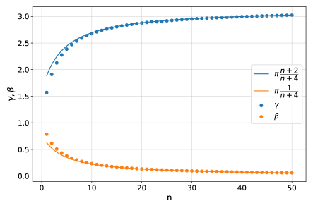
We now consider solutions for (8). For a given , it can be rewritten as a polynomial equation of power which does not have solutions in radicals. However, one can see that for , . We find correction to the asymptotic solution as , and calculate up to second order in . Thus for the optimal parameters:
| (9) | |||
| (10) |
Interestingly, solutions and , which turn into (9) and (10) for , approximate optimal parameters even for small (see Figure 1).
IV.2 Parameter concentration for
For the ansatz becomes:
| (12) |
The corresponding amplitude can be expressed in terms of the amplitude at from (4):
| (13) |
To find the parameters that maximize overlap , we set the gradients to zero and obtain a set of four equations. Even though in this case the variables do not separate, for solutions behave as:
| (14) |
Assuming and corrections to be of the next order in , we again search for parameters as and and obtain
| (15) | ||||
| (16) | ||||
| (17) | ||||
| (18) |
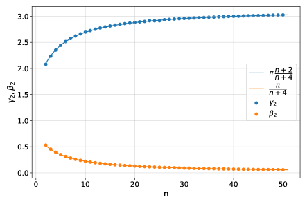
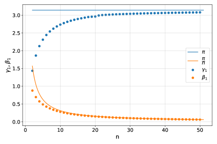
It is seen that parameters and behave in the same way as for the case in (9) and (10). Moreover, expressions and , which match our analytical solution for large , also fall within optimal approximation for (see Figure 2).
The corrections to the parameters and turn out to be of the next order in and so we do not calculate them explicitly. In comparison to optimal parameters recovered numerically, the analytical predictions (17) match optimal parameters beyond (see Figure 2).
Note that for large , corrections to parameters and are of third and second order respectively. But for any finite region in , parameters are well approximated by the functions
| (19) |
where the fitting constants and are region specific.
(a)
(b)
IV.3 Parameter concentration for
We have numerical evidence (up to and qubits) that for higher depths, optimal parameters also behave as (14) for large . Therefore, one might assume it to be a general feature. In order to calculate corrections for higher depth, the procedure described in the previous subsection can be used. However, a more straightforward approach is to Taylor-expand the overlap function around low-order solutions (14) up to second order in . This simplified expression is a quadratic form and thus can be maximized to obtain corrections.
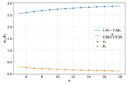
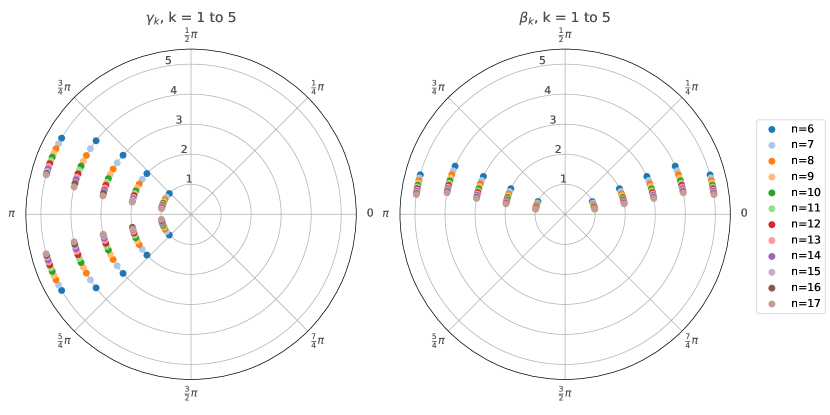
Below we present our numerical results for . Figure 3 demonstrates numerically calculated optimal parameters for the last layer. Optimal parameters at depth are fit according to (19) and the corresponding fit-constants appear in table I.
According to fitting curves which accurately describe the numerical data, parameter concentration is evident and is the same as in (20). We also plot our numerical data in Figure 4 to visually illustrate the phenomena of parameter concentration.
| , | ||||
| , | ||||
| , | ||||
| , | ||||
| , |
V Discussion
In present work we provide a rigorous definition of parameter concentrations and demonstrate it for the variational state preparation. The definition is motivated by how this effect can be leveraged for efficient training. However, different approaches claiming concentrations appear in the QAOA literature, yet our results have a clear distinction. Specifically Farhi2019a analytically addresses what we call instance concentration in the case of the Sherrington-Kirkpatrick model. Here, one finds that the variance in objective function value vanishes in the infinite size limit (), and therefore, QAOA becomes instance independent. However, the result alone neither predict nor address the behavior of optimal parameters.
Numerically in Streif2020 it is seen that the optimal parameters at each depth distribute over a small range when considering randomly generated MAX-CUT instances on 3-regular graphs. Moreover, this distribution became narrower as the system size increased. The authors in Streif2020 explain their numerical observation via reverse causal cone i.e. the subgraphs effectively contributing to the objective function when taken over a particular edge. Since in the limit , the likely subgraphs are trees, optimal parameters for QAOA on such subgraphs become optimal for the entire graph. However, the scaling behavior (if any) for the optimal parameters towards the infinite limit still remain lacking.
Although in our work only a unique set of optimal parameters is addressed at each , their scaling behavior is fully understood due to our analytical result. Furthermore, we expect our results to be applicable in more general settings which would imply that distribution of optimal parameters with respect to instances are only slightly sensitive if is large. Such an implication can be leveraged to reduce the training cost of finding optimal parameters.
In particular, our observed concentrations scale as , this implies optimal parameters also have a limit as . Therefore, one can train on a finite fraction qubits and perform a polynomially restricted training over optimal parameters at qubits to recover optimal parameters for qubits. However, to fully exploit this approach further investigation is needed.
Note that if parameters concentrate as with , optimal parameters may not approach any limit. In this case partial training at qubits may not guarantee optimality for qubits. However the existence of such cases remains to be observed.
Acknowledgements
The authors acknowledge support from the research project, Leading Research Center on Quantum Computing (agreement No. 014/20).
References
- (1) Matthew P Harrigan, Kevin J Sung, Matthew Neeley, Kevin J Satzinger, Frank Arute, Kunal Arya, Juan Atalaya, Joseph C Bardin, Rami Barends, Sergio Boixo, et al. Quantum approximate optimization of non-planar graph problems on a planar superconducting processor. Nature Physics, pages 1–5, 2021.
- (2) Guido Pagano, A Bapat, P Becker, KS Collins, A De, PW Hess, HB Kaplan, A Kyprianidis, WL Tan, C Baldwin, et al. Quantum approximate optimization of the long-range ising model with a trapped-ion quantum simulator. arXiv preprint arXiv:1906.02700, 2019.
- (3) Gian Giacomo Guerreschi and Anne Y Matsuura. Qaoa for max-cut requires hundreds of qubits for quantum speed-up. Scientific reports, 9(1):1–7, 2019.
- (4) Anastasiia Butko, George Michelogiannakis, Samuel Williams, Costin Iancu, David Donofrio, John Shalf, Jonathan Carter, and Irfan Siddiqi. Understanding quantum control processor capabilities and limitations through circuit characterization. In 2020 International Conference on Rebooting Computing (ICRC), pages 66–75. IEEE, 2020.
- (5) Edward Farhi, Jeffrey Goldstone, and Sam Gutmann. A Quantum Approximate Optimization Algorithm. nov 2014.
- (6) Murphy Yuezhen Niu, Sirui Lu, and Isaac L Chuang. Optimizing qaoa: Success probability and runtime dependence on circuit depth. arXiv preprint arXiv:1905.12134, 2019.
- (7) Seth Lloyd. Quantum approximate optimization is computationally universal. arXiv preprint arXiv:1812.11075, 2018.
- (8) Mauro ES Morales, JD Biamonte, and Zoltán Zimborás. On the universality of the quantum approximate optimization algorithm. Quantum Information Processing, 19(9):1–26, 2020.
- (9) Leo Zhou, Sheng Tao Wang, Soonwon Choi, Hannes Pichler, and Mikhail D. Lukin. Quantum Approximate Optimization Algorithm: Performance, Mechanism, and Implementation on Near-Term Devices. Physical Review X, 10(2):021067, jun 2020.
- (10) Zhihui Wang, Nicholas C Rubin, Jason M Dominy, and Eleanor G Rieffel. X y mixers: Analytical and numerical results for the quantum alternating operator ansatz. Physical Review A, 101(1):012320, 2020.
- (11) Lucas T. Brady, Christopher L. Baldwin, Aniruddha Bapat, Yaroslav Kharkov, and Alexey V. Gorshkov. Optimal Protocols in Quantum Annealing and Quantum Approximate Optimization Algorithm Problems. Physical Review Letters, 126(7):070505, feb 2021.
- (12) Edward Farhi and Aram W Harrow. Quantum Supremacy through the Quantum Approximate Optimization Algorithm. feb 2016.
- (13) V. Akshay, H. Philathong, M. E.S. Morales, and J. D. Biamonte. Reachability Deficits in Quantum Approximate Optimization. Physical Review Letters, 124(9):090504, mar 2020.
- (14) Edward Farhi, Jeffrey Goldstone, Sam Gutmann, and Leo Zhou. The Quantum Approximate Optimization Algorithm and the Sherrington-Kirkpatrick Model at Infinite Size. Technical report, 2019.
- (15) Matteo M. Wauters, Glen Bigan Mbeng, and Giuseppe E. Santoro. Polynomial scaling of QAOA for ground-state preparation of the fully-connected p-spin ferromagnet. mar 2020.
- (16) Jahan Claes and Wim van Dam. Instance Independence of Single Layer Quantum Approximate Optimization Algorithm on Mixed-Spin Models at Infinite Size. feb 2021.
- (17) Leo Zhou, Sheng-Tao Wang, Soonwon Choi, Hannes Pichler, and Mikhail D. Lukin. Quantum approximate optimization algorithm: Performance, mechanism, and implementation on near-term devices. Phys. Rev. X, 10:021067, Jun 2020.
- (18) Zhang Jiang, Eleanor G. Rieffel, and Zhihui Wang. Near-optimal quantum circuit for Grover’s unstructured search using a transverse field. Physical Review A, 95(6), feb 2017.
- (19) Matthew B Hastings. Classical and quantum bounded depth approximation algorithms. arXiv preprint arXiv:1905.07047, 2019.
- (20) Sergey Bravyi, Alexander Kliesch, Robert Koenig, and Eugene Tang. Obstacles to State Preparation and Variational Optimization from Symmetry Protection. Physical Review Letters, 125(26), oct 2019.
- (21) Ernesto Campos, Aly Nasrallah, and Jacob Biamonte. Abrupt transitions in variational quantum circuit training. Phys. Rev. A, 103:032607, Mar 2021.
- (22) Fernando GSL Brandao, Michael Broughton, Edward Farhi, Sam Gutmann, and Hartmut Neven. For fixed control parameters the quantum approximate optimization algorithm’s objective function value concentrates for typical instances. arXiv preprint arXiv:1812.04170, 2018.
- (23) Michael Streif and Martin Leib. Training the quantum approximate optimization algorithm without access to a quantum processing unit. Quantum Science and Technology, 5(3):34008, jul 2020.
- (24) Stefan H Sack and Maksym Serbyn. Quantum annealing initialization of the quantum approximate optimization algorithm. arXiv preprint arXiv:2101.05742, 2021.
- (25) Gavin E Crooks. Performance of the quantum approximate optimization algorithm on the maximum cut problem. arXiv preprint arXiv:1811.08419, 2018.
- (26) Jun Li, Xiaodong Yang, Xinhua Peng, and Chang Pu Sun. Hybrid Quantum-Classical Approach to Quantum Optimal Control. Physical Review Letters, 118(15):150503, apr 2017.
- (27) Constantin Brif, Raj Chakrabarti, and Herschel Rabitz. Control of quantum phenomena: Past, present and future. New Journal of Physics, 12(7):075008, jul 2010.
- (28) Arthur Larrouy, Sabrina Patsch, Rémi Richaud, Jean-Michel Raimond, Michel Brune, Christiane P. Koch, and Sébastien Gleyzes. Fast navigation in a large hilbert space using quantum optimal control. Phys. Rev. X, 10:021058, Jun 2020.
- (29) D. Leibfried. Quantum state preparation and control of single molecular ions. New Journal of Physics, 14(12pp):23029, feb 2012.
- (30) Kenji Sugisaki, Shigeaki Nakazawa, Kazuo Toyota, Kazunobu Sato, Daisuke Shiomi, and Takeji Takui. Quantum chemistry on quantum computers: A method for preparation of multiconfigurational wave functions on quantum computers without performing post-hartree–fock calculations. ACS Central Science, 5(1):167–175, 2019.
- (31) Frank Verstraete, Michael M. Wolf, and J. Ignacio Cirac. Quantum computation and quantum-state engineering driven by dissipation. Nature Physics, 5(9):633–636, jul 2009.
- (32) Christie S. Chiu, Geoffrey Ji, Anton Mazurenko, Daniel Greif, and Markus Greiner. Quantum State Engineering of a Hubbard System with Ultracold Fermions. Physical Review Letters, 120(24):243201, jun 2018.
- (33) K. Saito, M. Wubs, S. Kohler, P. Hänggi, and Y. Kayanuma. Quantum state preparation in circuit QED via Landau-Zener tunneling. Europhysics Letters, 76(1):22–28, oct 2006.
- (34) D. Gelbwaser-Klimovsky and G. Kurizki. Heat-machine control by quantum-state preparation: From quantum engines to refrigerators. Physical Review E - Statistical, Nonlinear, and Soft Matter Physics, 90(2):022102, aug 2014.
- (35) Andrey Kardashin, Alexey Uvarov, Dmitry Yudin, and Jacob Biamonte. Certified variational quantum algorithms for eigenstate preparation. Physical Review A, 102(5):052610, nov 2020.
- (36) Philip Richerme, Crystal Senko, Jacob Smith, Aaron Lee, Simcha Korenblit, and Christopher Monroe. Experimental performance of a quantum simulator: Optimizing adiabatic evolution and identifying many-body ground states. Physical Review A, 88(1):012334, 2013.
- (37) Hannes Bernien, Sylvain Schwartz, Alexander Keesling, Harry Levine, Ahmed Omran, Hannes Pichler, Soonwon Choi, Alexander S Zibrov, Manuel Endres, Markus Greiner, et al. Probing many-body dynamics on a 51-atom quantum simulator. Nature, 551(7682):579–584, 2017.
- (38) Michael Streif and Martin Leib. Comparison of qaoa with quantum and simulated annealing. arXiv preprint arXiv:1901.01903, 2019.
- (39) Wen Wei Ho and Timothy H Hsieh. Efficient unitary preparation of non-trivial quantum states. arXiv preprint arXiv:1803.00026, 2018.
- (40) Wen Wei Ho, Cheryne Jonay, and Timothy H. Hsieh. Ultrafast variational simulation of nontrivial quantum states with long-range interactions. Phys. Rev. A, 99:052332, May 2019.
- (41) Andreas Bartschi and Stephan Eidenbenz. Grover Mixers for QAOA: Shifting Complexity from Mixer Design to State Preparation. In Proceedings - IEEE International Conference on Quantum Computing and Engineering, QCE 2020, pages 72–82. Institute of Electrical and Electronics Engineers Inc., oct 2020.
- (42) Viacheslav V. Kuzmin and Pietro Silvi. Variational quantum state preparation via quantum data buses. Quantum, 4:1–15, jul 2020.
- (43) Abhinav Kandala, Antonio Mezzacapo, Kristan Temme, Maika Takita, Markus Brink, Jerry M Chow, and Jay M Gambetta. Hardware-efficient variational quantum eigensolver for small molecules and quantum magnets. Nature, 549(7671):242–246, 2017.