Finiteness of Stationary Configurations of the Planar Five-vortex Problem

Abstract

For the planar five-vortex problem, we show that there are finitely many relative equilibria (uniformly rotating configurations) and collapse configurations, except perhaps if the vorticities satisfy some explicitly given algebraic constraints. In particular, if the vorticities are of the same sign, we show the number of relative equilibria and collapse configurations are finite.

Keywords: Point vortices; Relative equilibrium; Finiteness.

2020AMS Subject Classification 76B47 70F10 70F15 37Nxx .

1 Introduction

The planar $N$-vortex problem, dated back to Helmholtz’s work on hydrodynamics in 1858 [6], consider the dynamical system given by

$$\Gamma_{n}\dot{\mathbf{r}}_{n}=J\nabla_{k}H=J\sum_{1\leq j\leq N,j\neq n}\frac{\Gamma_{n}\Gamma_{j}(\mathbf{r}_{j}-\mathbf{r}_{n})}{|\mathbf{r}_{j}-\mathbf{r}_{n}|^{2}},~{}~{}~{}~{}~{}~{}~{}~{}~{}~{}~{}~{}~{}~{}~{}n=1,2,\cdots,N.$$ (1.1)

where $\Gamma_{n}\in\mathbb{R}\backslash\{0\}$ is the vortex strength (or vorticity) and $\mathbf{r}_{n}\in{\mathbb{R}}^{2}$ is the position for $n=1,...,N$, $J=\left(\begin{array}[]{cc}0&1\\ -1&0\\ \end{array}\right)$, $H=-\sum_{1\leq j<k\leq N}\ln|\mathbf{r}_{j}-\mathbf{r}_{k}|$, and $|\cdot|$ denotes the Euclidean norm in ${\mathbb{R}}^{2}$.

It is of physical interest to study stationary configurations which lead to self-similar solutions of the $N$-vortex problem[10, 14]. O’Neil [10] has shown that the only stationary configurations are equilibria, rigidly translating configurations, relative equilibria (uniformly rotating configurations) and collapse configurations.

For two and three vorticities, stationary configurations are known to be finite, [4, 13, 8, 9, 2, 3]. For four vorticities, O’Neil [11], Hampton and Moeckel [5] independently proved that the numbers of equilibria, rigidly translating configurations and relative equilibria are generically finite. However, their methods do not work for collapse configurations.

Motivated by the novel method of Albouy and Kaloshin for celestial mechanics [1], the first author introduced a system of equations (2.7), whose solution set contains relative equilibria and collapse configurations. The system would admit a continuum of complex solutions if there are infinitely many relative equilibria and collapse configurations. Then the finiteness of all stationary configurations for the 4-vortex problem is established by analysis of the singularities of the system [14].

In this study, we shall apply the method introduced in [14] to study the finiteness problem of relative equilibria and collapse configurations for the five-vortex problem. Because of the well-known continuum of relative equilibria [12], (see Section 2), the finiteness of relative equilibria and collapse configurations would be expected only for generic vorticities. We have proven the following results:

Theorem 1.1

If the vorticities $\Gamma_{n}$ $(n\in\{1,2,3,4,5\})$ are nonzero, the five-vortex problem has finitely many relative equilibria and collapse configurations, with the possible exception of some vorticity parameter values on which an explicitly given set of polynomials vanish (see Sect. 5).

Theorem 1.2

For any choice of five vorticities, if $\sum_{j\in J}\Gamma_{j}\neq 0$ and $\sum_{j,k\in J,j\neq k}\Gamma_{j}\Gamma_{k}\neq 0$, where $J$ is a nonempty subset of $\{1,2,3,4,5\}$, there are finitely many normalized central configurations of the five-vortex problem.

Corollary 1.3

If the vorticity $\Gamma_{n}$ $(n\in\{1,2,3,4,5\})$ are all positive (or negative), then the five-vortex problem has finitely many relative equilibria and collapse configurations.

Recall that in the Newtonian five-body problem, even the masses are all positive, there exists a continuum of central configurations in the complex domain [1]. Theorem 1.2 points out one of the many differences between central configurations of the Newtonian five-body problem and that of the five-vortex problem when finiteness of central configurations is concerned.

The paper is structured as follows. In Section 2, we give some notations and definitions. In particular, following Albouy and Kaloshin [1], we introduce singular sequences of normalized central configurations. In Section 3, we discuss some tools to classify the singular sequences. In Section 4, we study all possible singular sequences and reduce the problem to twenty-nine diagrams. In Section 5, we obtain the constraints on the vorticities corresponding to each of the twenty-nine diagrams. In Section 6, we prove Theorem 1.1 and Theorem 1.2.

2 Preliminaries

In this section we recall some notations and definitions that will be needed later.

2.1 Stationary configurations

First it is more convenient to consider the vortex positions $\mathbf{r}_{n}\in\mathbb{R}^{2}$ as complex numbers $z_{n}\in\mathbb{C}$, in which case the dynamics are given by $\dot{z}_{n}=-\textbf{i}V_{n}$ where

$$V_{n}=\sum_{1\leq j\leq N,j\neq n}\frac{\Gamma_{j}z_{jn}}{r_{jn}^{2}}=\sum_{j\neq n}\frac{\Gamma_{j}}{{\overline{z}_{jn}}},$$ (2.2)

$z_{jn}=z_{n}-z_{j}$, $r_{jn}=|z_{jn}|=\sqrt{z_{jn}{\overline{z}_{jn}}}$, $\textbf{i}=\sqrt{-1}$ and the over bar denotes complex conjugation.

Let $\mathbb{C}^{N}=\{z=(z_{1},\cdots,z_{N}):z_{j}\in\mathbb{C},j=1,\cdots,N\}$ denote the space of configurations for $N$ point vortex. Let $\Delta=\{z\in\mathbb{C}^{N}:z_{j}=z_{k}~{}~{}\emph{for some}~{}~{}j\neq k\}$ be the collision set in $\mathbb{C}^{N}$. Then the set $\mathbb{C}^{N}\backslash\Delta$ is the space of collision-free configurations.

Definition 2.1

The following quantities are defined:

$\begin{array}[]{cc}\text{Total vorticity}&\Gamma=\sum_{j=1}^{N}\Gamma_{j}\\ \text{Total vortex angular momentum}&L=\sum_{1\leq j<k\leq N}\Gamma_{j}\Gamma_{k}\\ \text{ Moment of vorticity }&M=\sum_{j=1}^{N}\Gamma_{j}z_{j}\\ \text{ Angular impulse }&I=\sum_{j=1}^{N}\Gamma_{j}|z_{j}|^{2}=\sum_{j=1}^{N}\Gamma_{j}z_{j}{\overline{z}_{j}}\end{array}$

Then it is easy to see that

$$\Gamma I=\sum_{1\leq j<k\leq N}\Gamma_{j}\Gamma_{k}z_{jk}{\overline{z}_{jk}}=\sum_{1\leq j<k\leq N}\Gamma_{j}\Gamma_{k}r_{jk}^{2}\triangleq S,$$ (2.3)

and

$$\Gamma^{2}-2L>0.$$ (2.4)

Following O’Neil [10] we will call a configuration stationary if the relative shape remains constant, i.e., if the ratios of mutual distances $r_{jk}/r_{lm}$ remain constant (such solutions are often called homographic). More precisely,

Definition 2.2

A configuration $z\in\mathbb{C}^{N}\backslash\Delta$ is stationary if there exists a constant $\Lambda\in{\mathbb{C}}$ such that

$$V_{j}-V_{k}=\Lambda(z_{j}-z_{k}),~{}~{}~{}~{}~{}~{}~{}~{}~{}~{}1\leq j,k\leq N.$$ (2.5)

It is shown that the only stationary configurations of vortices are equilibria, rigidly translating configurations, relative equilibria (uniformly rotating configurations) and collapse configurations [10].

Definition 2.3

• $z\in\mathbb{C}^{N}\backslash\Delta$ is an equilibrium if $V_{1}=\cdots=V_{N}=0$.

• $z\in\mathbb{C}^{N}\backslash\Delta$ is rigidly translating if $V_{1}=\cdots=V_{N}=V$ for some $V\in\mathbb{C}\backslash\{0\}$. (The vortices are said to move with common velocity $V$.)

• $z\in\mathbb{C}^{N}\backslash\Delta$ is a relative equilibrium if there exist constants $\lambda\in\mathbb{R}\backslash\{0\},z_{0}\in\mathbb{C}$ such that $V_{n}=\lambda(z_{n}-z_{0}),~{}~{}~{}~{}~{}~{}~{}~{}~{}~{}1\leq n\leq N$.

• $z\in\mathbb{C}^{N}\backslash\Delta$ is a collapse configuration if there exist constants $\Lambda,z_{0}\in\mathbb{C}$ with $\emph{Im}(\Lambda)\neq 0$ such that $V_{n}=\Lambda(z_{n}-z_{0}),~{}~{}~{}~{}~{}~{}~{}~{}~{}~{}1\leq n\leq N$.

It is easy to see that $L=0$ is a necessary condition for the existence of equilibria, and $\Gamma=0$ is a necessary condition for the existence of configurations [10].

Proposition 2.1

Every equilibrium has vorticities satisfying $L=0$; every rigidly translating configuration has vorticities satisfying $\Gamma=0$

If $z^{\prime}$ differs from $z$ only by translation, rotation, and change of scale (dilation) in the plane, then it is easy to see that $z$ is stationary if and only if $z^{\prime}$ is stationary.

Definition 2.4

A configuration $z$ is equivalent to a configuration $z^{\prime}$ if for some $a,b\in\mathbb{C}$ with $b\neq 0$, $z^{\prime}_{n}=b(z_{n}+a),~{}~{}~{}1\leq n\leq N$.

$z\in\mathbb{C}^{N}\backslash\Delta$ is a translation-normalized configuration if $M=0$; $z\in\mathbb{C}^{N}\backslash\Delta$ is a rotation-normalized configuration if $z_{12}\in\mathbb{R}$. Fixing the scale of a configuration, we can give the definition of dilation-normalized configuration, however, we do not specify the scale here.

A configuration, which is translation-normalized, rotation-normalized and dilation-normalized, is called a normalized configuration.

Note that for a given configuration $z$, there always is certain rotation-normalized configuration and dilation-normalized configuration being equivalent to $z$; if $\Gamma\neq 0$, then there is always certain translation-normalized configuration being equivalent to $z$ too. Hence, if $\Gamma\neq 0$, there is exactly one normalized configuration being equivalent to $z$.

2.2 Central configurations

In this paper we consider only relative equilibria and collapse configurations, then it is easy to see that there always is certain translation-normalized configuration being equivalent to a given configuration.

The equations of relative equilibria and collapse configurations can be unified into the following formula

$$V_{n}=\Lambda(z_{n}-z_{0}),~{}~{}~{}~{}~{}~{}~{}~{}~{}~{}1\leq n\leq N,$$ (2.6)

$\Lambda\in\mathbb{R}\backslash\{0\}$ corresponds to relative equilibria and $\Lambda\in\mathbb{C}\backslash\mathbb{R}$ corresponds to collapse configurations.

Definition 2.5

Relative equilibria and collapse configurations are both called central configurations.

The equations (2.6) can be reducible to

$$\Lambda z_{n}=V_{n},~{}~{}~{}~{}~{}~{}~{}~{}~{}~{}1\leq n\leq N,$$ (2.7)

if we replace $z_{n}$ by $z_{n}+z_{0}$, i.e., the solutions of equations (2.7) have been removed the translation freedoms. In fact, it is easy to see that the solutions of equations (2.7) satisfy

$$M=0,$$ (2.8)

$$\Lambda I=L.$$ (2.9)

To remove the dilation freedoms, we set $|\Lambda|=1$. Following Albouy and Kaloshin [1] we introduce

Definition 2.6

A real normalized central configuration of the planar $N$-vortex problem is a solution of (2.7) satisfying $z_{12}\in\mathbb{R}$ and $|\Lambda|=1$.

We remark that we shall study system (2.7) in the complex domain and the word “real” refers to the reality hypothesis. It is omitted in a real context.

Proposition 2.2

[14] Collapse configurations satisfy $\Gamma\neq 0$ and

$$S=I=L=0.$$ (2.10)

For relative equilibria we have $S=0~{}~{}~{}\Longleftrightarrow~{}~{}~{}\left\{\begin{array}[]{lr}\Gamma\neq 0&\\ I=L=0&\end{array}\right.\text{or}~{}~{}~{}\left\{\begin{array}[]{lr}\Gamma=0&\\ I\neq 0,L\neq 0&\end{array}\right.$

2.3 Complex central configurations

To eliminate complex conjugation in (2.7) we introduce a new set of variables $w_{n}$ and a “conjugate” relation:

$$\begin{array}[]{c}\Lambda z_{n}=\sum_{j\neq n}\frac{\Gamma_{j}}{{w_{jn}}},~{}~{}~{}~{}~{}~{}~{}~{}~{}~{}1\leq n\leq N,\\ \overline{\Lambda}w_{n}=\sum_{j\neq n}\frac{\Gamma_{j}}{{z_{jn}}},~{}~{}~{}~{}~{}~{}~{}~{}~{}~{}1\leq n\leq N,\end{array}$$ (2.11)

where $z_{jn}=z_{n}-z_{j}$ and $w_{jn}=w_{n}-w_{j}$.

The rotation freedom is expressed in $z_{n},w_{n}$ variables as the invariance of (2.11) by the map $R_{a}:(z_{n},w_{n})\mapsto(az_{n},a^{-1}w_{n})$ for any $a\in\mathbb{C}\backslash\{0\}$ and any $n=1,2,\cdots,N$. The condition $z_{12}\in\mathbb{R}$ we proposed to remove this rotation freedom becomes $z_{12}=w_{12}$.

To the variables $z_{n},w_{n}\in\mathbb{C}$ we add the variables $Z_{jk},W_{jk}\in\mathbb{C}$ $(1\leq j<k\leq N)$ such that $Z_{jk}=1/w_{jk},W_{jk}=1/z_{jk}$. For $1\leq k<j\leq N$ we set $Z_{jk}=-Z_{kj},W_{jk}=-W_{kj}$. Then equations (2.7) together with the condition $z_{12}\in\mathbb{R}$ and $|\Lambda|=1$ becomes

$$\begin{array}[]{cc}\Lambda z_{n}=\sum_{j\neq n}\Gamma_{j}Z_{jn},&1\leq n\leq N,\\ \overline{\Lambda}w_{n}=\Lambda^{-1}w_{n}=\sum_{j\neq n}\Gamma_{j}W_{jn},&1\leq n\leq N,\\ Z_{jk}w_{jk}=1,&1\leq j<k\leq N,\\ W_{jk}z_{jk}=1,&1\leq j<k\leq N,\\ z_{jk}=z_{k}-z_{j},~{}~{}~{}w_{jk}=w_{k}-w_{j},&1\leq j,k\leq N,\\ Z_{jk}=-Z_{kj},~{}~{}~{}W_{jk}=-W_{kj},&1\leq k<j\leq N,\\ z_{12}=w_{12}.\end{array}$$ (2.12)

This is a polynomial system in the variables $\mathcal{Q}=(\mathcal{Z},\mathcal{W})\in(\mathbb{C}^{N}\times\mathbb{C}^{N(N-1)/2})^{2}$, here

$\mathcal{Z}=(z_{1},z_{2},\cdots,z_{N},Z_{12},Z_{13},\cdots,Z_{(N-1)N})$, $\mathcal{W}=(w_{1},w_{2},\cdots,w_{N},W_{12},W_{13},\cdots,W_{(N-1)N}).$

It is easy to see that a real normalized central configuration of (2.7) is a solution $\mathcal{Q}=(\mathcal{Z},\mathcal{W})$ of (2.12) such that $z_{n}={\overline{w}}_{n}$ and vice versa.

Definition 2.7 (Normalized central configuration)

A normalized central configuration is a solution $\mathcal{Q}=(\mathcal{Z},\mathcal{W})$ of (2.12). A real normalized central configuration is a normalized central configuration such that $z_{n}={\overline{w}}_{n}$ for any $n=1,2,\cdots,N$.

Definition 2.7 of a real normalized central configuration coincides with Definition 2.6.

Definition 2.8

We will use the name “distance” for the $r_{jk}=\sqrt{z_{jk}{w_{jk}}}$. We will use the name $z$-separation (respectively $w$-separation) for the $z_{jk}$’s (respectively the $w_{jk}$’s) in the complex plane.

Strictly speaking, the distances $r_{jk}=\sqrt{z_{jk}{w_{jk}}}$ are now bi-valued. However, only the squared distances appear in the system, so we shall understand $r^{2}_{jk}$ as $z_{jk}w_{jk}$ from now on.

2.4 Elimination theory

Let $m$ be a positive integer. Following [7], we define a closed algebraic subset of the affine space $\mathbb{C}^{m}$ as the set of common zeros of a system of polynomials on $\mathbb{C}^{m}$.

The polynomial system (2.12) defines a closed algebraic subset $\mathcal{A}\subset(\mathbb{C}^{N}\times\mathbb{C}^{N(N-1)/2})^{2}$. For the planar five-vortex problem, we will prove that this subset is finite, then real normalized central configurations is finite. To distinguish the two possibilities, finitely many or infinitely many points, we will only use the following result (see [1]) from elimination theory.

Lemma 2.1

Let $\mathcal{X}$ be a closed algebraic subset of $\mathbb{C}^{m}$ and $f:\mathbb{C}^{m}\rightarrow\mathbb{C}$ be a polynomial. Either the image $F(\mathcal{X})\subset\mathbb{C}$ is a finite set, or it is the complement of a finite set. In the second case one says that f is dominating.

2.5 Singular sequences of normalized central configurations

We consider a solution $\mathcal{Q}=(\mathcal{Z},\mathcal{W})$ of (2.12), this is a normalized central configuration. Let $\mathfrak{N}=N(N+1)/2$. Set

$\mathcal{Z}=(\mathcal{Z}_{1},\mathcal{Z}_{2},\cdots,\mathcal{Z}_{\mathfrak{N}})=(z_{1},z_{2},\cdots,z_{N},Z_{12},Z_{13},\cdots,Z_{(N-1)N})$,

$\mathcal{W}=(\mathcal{W}_{1},\mathcal{W}_{2},\cdots,\mathcal{W}_{\mathfrak{N}})=(w_{1},w_{2},\cdots,w_{N},W_{12},W_{13},\cdots,W_{(N-1)N})$.

Let $\|\mathcal{Z}\|=\max_{j=1,2,\cdots,\mathfrak{N}}|\mathcal{Z}_{j}|$ be the modulus of the maximal component of the vector $\mathcal{Z}\in\mathbb{C}^{\mathfrak{N}}$. Similarly, set $\|\mathcal{W}\|=\max_{k=1,2,\cdots,\mathfrak{N}}|\mathcal{W}_{k}|$.

Consider a sequence $\mathcal{Q}^{(n)}$, $n=1,2,\cdots$, of normalized central configurations. Extract a sub-sequence such that the maximal component of $\mathcal{Z}^{(n)}$ is always the same, i.e., $\|\mathcal{Z}^{(n)}\|=|\mathcal{Z}^{(n)}_{j}|$ for a $j\in\{1,2,\cdots,\mathfrak{N}\}$ that does not depend on $n$. Extract again in such a way that the vector sequence $\mathcal{Z}^{(n)}/\|\mathcal{Z}^{(n)}\|$ converges. Extract again in such a way that there is similarly an integer $k\in\{1,2,\cdots,\mathfrak{N}\}$ such that $\|\mathcal{W}^{(n)}\|=|\mathcal{W}^{(n)}_{k}|$ for all $n$. Extract a last time in such a way that the vector sequence $\mathcal{W}^{(n)}/\|\mathcal{W}^{(n)}\|$ converges.

If the initial sequence is such that $\mathcal{Z}^{(n)}$ or $\mathcal{W}^{(n)}$ is unbounded, so is the extracted sequence. Note that $\|\mathcal{Z}^{(n)}\|$ and $\|\mathcal{W}^{(n)}\|$ are bounded away from zero: if the first $N$ components of the vector $\mathcal{Z}^{(n)}$ or $\|\mathcal{W}^{(n)}\|$ all go to zero, then the denominator $z_{12}=w_{12}$ of the component $Z_{12}=W_{12}$ go to zero and $\mathcal{Z}^{(n)}$ and $\mathcal{W}^{(n)}$ are unbounded. There are two possibilities for the extracted sub-sequences above:

• $\mathcal{Z}^{(n)}$ and $\mathcal{W}^{(n)}$ are bounded,

• at least one of $\mathcal{Z}^{(n)}$ and $\mathcal{W}^{(n)}$ is unbounded.

Definition 2.9 (Singular sequence)

Consider a sequence of normalized central configurations. A sub-sequence extracted by the above process, in the unbounded case, is called a singular sequence.

Robert’s continuum. Roberts found the following continuum of relative equilibria for five vortices. The masses are $m_{1}=m_{2}=m_{3}=m_{4}=2,m_{5}=-1$. The fifth vortex is at the origin $z_{5}=w_{5}=0$, while the first four vortices form a rhombus

$$(z_{1},z_{2},z_{3},z_{4})=(a,b,-a,-b),\ (w_{1},w_{2},w_{3},w_{4})=(a,-b,-a,b),\$$

where $a\in\mathbb{R}$ and $\textbf{i}b\in\mathbb{R}$ for the real configurations. One can check that the configuration defined by the coordinates above and the restriction $r^{2}_{12}=r^{2}_{23}=r^{2}_{34}=r^{2}_{14}=a^{2}-b^{2}=1$ satisfies system (2.12).

For the real configurations, when $a\to 0$, vertices 1, 3, and 5 collide; when $b\to 0$, vertices 2, 4, and 5 collide. We get a real triple contact “singularity”. For the complex configurations, when $a\to\infty$, we have two choices: $b\sim a$ or $b\sim-a$. We get two other singularities at imaginary infinity.

3 Tools to classify the singular sequences

Definition 3.1 (Notation of asymptotic estimates)

$a\sim b$

means $a/b\rightarrow 1$

$a\prec b$

means $a/b\rightarrow 0$

$a\preceq b$

means $a/b$ is bounded

$a\approx b$

means $a\preceq b$ and $a\succeq b$

Definition 3.2 (Strokes and circles.)

We pick a singular sequence. We write the indices of the bodies in a figure and use two colors for edges and vertices.

The first color, the $z$-color, is used to mark the maximal order components of

$\mathcal{Z}=(z_{1},z_{2},\cdots,z_{N},Z_{12},Z_{13},\cdots,Z_{(N-1)N})$.

They correspond to the components of the converging vector sequence $\mathcal{Z}^{(n)}/\|\mathcal{Z}^{(n)}\|$ that do not tend to zero. We draw a circle around the name of vertex j if the term $z^{(n)}_{j}$ is of maximal order among all the components of $\mathcal{Z}^{(n)}$. We draw a stroke between the names k and l if the term $Z^{(n)}_{kl}$ is of maximal order among all the components of $\mathcal{Z}^{(n)}$.

3.1 Rules of colored diagram

The following rules mainly concern $z$-diagram, but they apply as well to the $w$-diagram.

If there is a maximal order term in an equation, there should be another one. This gives immediately the following Rule I.

Rule I

There is something at each end of any $z$-stroke: another $z$-stroke or/and a $z$-circle drawn around the name of the vertex. A $z$-circle cannot be isolated; there must be a $z$-stroke emanating from it. There is at least one $z$-stroke in the $z$-diagram.

Definition 3.3 ($z$-close)

Consider a singular sequence. We say that bodies k and l are close in $z$-coordinate, or $z$-close, or that $z_{k}$ and $z_{l}$ are close, if $z^{(n)}_{kl}\prec\|\mathcal{Z}^{(n)}\|$.

The following statement is obvious.

Rule II

If bodies k and l are $z$-close, they are both $z$-circled or both not $z$-circled.

Definition 3.4 (Isolated component)

An isolated component of the $z$-diagram is a subset of vertices such that no $z$-stroke is joining a vertex of this subset to a vertex of the complement.

Rule III

The moment of vorticity of a set of bodies forming an isolated component of the $z$-diagram is $z$-close to the origin.

Rule IV

Consider the $z$-diagram or an isolated component of it. If there is a $z$-circled vertex, there is another one. The $z$-circled vertices can all be $z$-close together only if the total vorticity of these vertices is zero.

Definition 3.5 (Maximal $z$-stroke)

Consider a $z$-stroke from vertex k to vertex l. We say it is a maximal $z$-stroke if k and l are not $z$-close.

Rule V

There is at least one $z$-circle at certain end of any maximal $z$-stroke. As a result, if an isolated component of the $z$-diagram has no $z$-circled vertex, then it has no maximal $z$-stroke.

On the same diagram we also draw $w$-strokes and $w$-circles. Graphically we use another color. The previous rules and definitions apply to $w$-strokes and $w$-circles. What we will call simply the diagram is the superposition of the $z$-diagram and the $w$-diagram. We will, for example, adapt Definition 3.4 of an isolated component: a subset of bodies forms an isolated component of the diagram if and only if it forms an isolated component of the $z$-diagram and an isolated component of the $w$-diagram.

Definition 3.6 (Edges and strokes)

There is an edge between vertex k and vertex l if there is either a $z$-stroke, or a $w$-stroke, or both. There are three types of edges, $z$-edges, $w$-edges and $zw$-edges, and only two types of strokes, represented with two different colors.

Figure 1: A $z$-stroke, a $z$-stroke plus a $z$-stroke, a $w$-stroke, forming respectively a $z$-edge, a $zw$-edge, a $w$-edge.

3.1.1 New normalization. Main estimates.

One does not change a central configuration by multiplying the $z$ coordinates by $a\in\mathbb{C}\backslash\{0\}$ and the $w$ coordinates by $a^{-1}$. Our diagram is invariant by such an operation, as it considers the $z$-coordinates and the $z$-coordinates separately.

We used the normalization $z_{12}=w_{12}$ in the previous considerations. In the following we will normalize instead with $\|\mathcal{Z}\|=\|\mathcal{W}\|$. We start with a central configuration normalized with the condition $z_{12}=w_{12}$, then multiply the $z$-coordinates by $a>0$, the $w$-coordinates by $a^{-1}$, in such a way that the maximal component of $\mathcal{Z}$ and the maximal component of $\mathcal{W}$ have the same modulus, i.e., $\|\mathcal{Z}\|=\|\mathcal{W}\|$.

A singular sequence was defined by the condition either $\|\mathcal{Z}^{(n)}\|\rightarrow\infty$ or $\|\mathcal{W}^{(n)}\|\rightarrow\infty$. We also remarked that both $\|\mathcal{Z}^{(n)}\|$ and $\|\mathcal{W}^{(n)}\|$ were bounded away from zero. With the new normalization, a singular sequence is simply characterized by $\|\mathcal{Z}^{(n)}\|=\|\mathcal{W}^{(n)}\|\rightarrow\infty$. From now on we only discuss singular sequences.

Set $\|\mathcal{Z}^{(n)}\|=\|\mathcal{W}^{(n)}\|=1/\epsilon^{2}$, then $\epsilon\rightarrow 0$.

Proposition 3.1 (Estimate)

For any $(k,l)$, $1\leq k<l\leq N$, we have $\epsilon^{2}\preceq z_{kl}\preceq\epsilon^{-2}$, $\epsilon^{2}\preceq w_{kl}\preceq\epsilon^{-2}$ and $\epsilon^{2}\preceq r_{kl}\preceq\epsilon^{-2}$.

There is a $z$-stroke between k and l if and only if $w_{kl}\approx\epsilon^{2}$, then $r_{kl}\preceq 1$.

There is a maximal $z$-stroke between k and l if and only if $z_{kl}\approx\epsilon^{-2},w_{kl}\approx\epsilon^{2}$, then $r_{kl}\preceq 1$.

There is a $z$-edge between k and l if and only if $z_{kl}\succ\epsilon^{2},w_{kl}\approx\epsilon^{2}$, then $\epsilon^{2}\prec r_{kl}\preceq 1$.

There is a maximal $z$-edge between k and l if and only if $z_{kl}\approx\epsilon^{-2},w_{kl}\approx\epsilon^{2}$, then $r_{kl}\approx 1$.

There is a $zw$-edge between k and l if and only if $z_{kl},w_{kl}\approx\epsilon^{2}$, this can be characterized as $r_{kl}\approx\epsilon^{2}$.

Remark 3.1

By the estimates above, the strokes in a $zw$-edge are not maximal. A maximal $z$-stroke is exactly a maximal $z$-edge.

Circling method. Estimate show that in all the cases where there is a $z$-stroke between vertices k and l, there bodies are close in $w$-coordinate. Then Rule II applies to the $w$-diagram. Vertices k and l are both $w$-circled or both not $w$-circled. One vertex isolated in $w$-diagram can not be $w$-circled. If there is one $w$-circle, there is another $w$-circle.

Rule VI

If there are two consecutive $z$-stroke, there is a third $z$-stroke closing the triangle.

The Roberts’ continuum example produces the following collection of diagrams from left to right: $a\to 0$ and 1, 3, 5 collide; $b\to 0$ and 2, 4, 5 collide; $a\to\infty$ and $b\sim a$; $a\to\infty$ and $b\sim-a$, (see Figure 2).

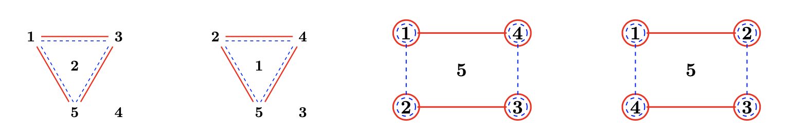
Figure 2: Roberts’ continuum at real triple contact and infinity

4 The possible diagrams

In this section, under the assumption that the total vorticity is nonvanishing and that each vorticity is nonzero, we derive a list of problematic diagrams. This list of twenty-nine diagrams is in Figure 16.

As in the case of the 5-body problem [1] in celestial mechanics, we divide possible diagrams into groups according to the maximal number of strokes from a bicolored vertex. During the analysis of all the possibilities we rule some of them out immediately, some with further arguments. The ones we cannot exclude without further hypotheses on the vorticities are incorporated into the list of twenty-nine in Figure 16.

We list some useful results.

Proposition 4.1

[14] Suppose a diagram has two $z$-circled vertices (say 1 and 2) which are also $z$-close, if none of all the other vertices is $z$-close with them, then $\Gamma_{1}+\Gamma_{2}\neq 0$ and $\overline{\Lambda}z_{12}w_{12}\sim\frac{1}{\Gamma_{1}+\Gamma_{2}}$. In particular, vertices 1 and 2 cannot form a $z$-stroke.

Proposition 4.2

[14] Consider an isolated component of the $z$-diagram. If the $z$-circled vertices are all $z$-close (for example, connected by $w$-strokes), then the total vorticity of these vertices is zero.

Proposition 4.3

[14] Suppose a diagram has an isolated $z$-color triangle, and none of vertices (say 1,2,3) of it are $z$-circled, then $L_{123}=\Gamma_{1}\Gamma_{2}+\Gamma_{2}\Gamma_{3}+\Gamma_{3}\Gamma_{1}=0$.

Proposition 4.4

[14] Suppose a fully $z$-stroked sub-diagram with four vertices exists in isolation in a diagram, and none of vertices (say 1,2,3,4) of it are $z$-circled, then

$$L_{1234}=\Gamma_{1}\Gamma_{2}+\Gamma_{2}\Gamma_{3}+\Gamma_{3}\Gamma_{1}+\Gamma_{4}(\Gamma_{1}+\Gamma_{2}+\Gamma_{3})=0.$$ (4.13)

Proposition 4.5

Suppose a diagram has one $z$-stroke that is isolated in the $z$-diagram and the two ends are $z$-circled. Call 1 and 2 the ends of this $z$-stoke. Suppose that there is no other $z$-circle in the diagram. Then $\Gamma_{1}+\Gamma_{2}\neq 0$. The diagram forces $\Lambda=\pm 1$ or $\pm\textbf{i}$. Furthermore,

• If $\Lambda=\pm 1$, we have $\sum_{j=3}^{N}\Gamma_{j}=0$;

• If $\Lambda=\pm\textbf{i}$, we have $L=0$ and $\Gamma_{1}\Gamma_{2}=L_{3...N}$.

Proof 1

First, if $\Gamma_{1}+\Gamma_{2}=0$, then two $z$-circled vertices 1 and 2 are $z$-close since $\Gamma_{1}z_{1}+\Gamma_{2}z_{2}=(\Gamma_{1}+\Gamma_{2})z_{1}+\Gamma_{2}(z_{2}-z_{1})<\epsilon^{-2}$. However, this contradicts Proposition 4.1. Thus $\Gamma_{1}+\Gamma_{2}\neq 0$.

Without loss of generality, assume $z_{1}\sim-\Gamma_{2}a\epsilon^{-2}$ and $z_{2}\sim\Gamma_{1}a\epsilon^{-2}$, then

$$z_{12}\sim(\Gamma_{1}+\Gamma_{2})a\epsilon^{-2},\ \frac{1}{z_{2}}-\frac{1}{z_{1}}\sim(\frac{1}{\Gamma_{1}}+\frac{1}{\Gamma_{2}})\frac{\epsilon^{2}}{a}.$$

The equations (2.12) gives

$$\begin{array}[]{c}\overline{\Lambda}w_{12}\sim(\Gamma_{1}+\Gamma_{2})W_{12}+\sum_{j=3}^{N}\Gamma_{j}(\frac{1}{z_{j2}}-\frac{1}{z_{j1}})\cr\Lambda z_{2}\sim\Gamma_{1}Z_{12}.\end{array}{}$$ (4.14)

The second equation of (4.14) gives $w_{12}\sim\frac{\epsilon^{2}}{a\Lambda}$. Note that $\frac{1}{z_{j2}}-\frac{1}{z_{j1}}\sim\frac{1}{z_{2}}-\frac{1}{z_{1}}$ for any $j>2$ and that $W_{12}=\frac{1}{z_{12}}$. The first equation of (4.14) leads to

$${\overline{\Lambda}}/{\Lambda}=1+\sum_{j=3}^{N}\Gamma_{j}(\frac{1}{\Gamma_{1}}+\frac{1}{\Gamma_{2}}).$$ (4.15)

It follows that $\Lambda=\pm 1$ or $\pm\textbf{i}$.

If $\Lambda=\pm 1$, we have

$$0=\sum_{j=3}^{N}\Gamma_{j}(\frac{1}{\Gamma_{1}}+\frac{1}{\Gamma_{2}}),\ \Rightarrow\ \sum_{j=3}^{N}\Gamma_{j}=0.$$

If $\Lambda=\pm\textbf{i}$, we have

$$-2=\sum_{j=3}^{N}\Gamma_{j}(\frac{1}{\Gamma_{1}}+\frac{1}{\Gamma_{2}}),\ L=0,\ \Rightarrow L=0,\ \Gamma_{1}\Gamma_{2}=L_{3...N}.$$

Similarly, we have the following result.

Proposition 4.6

Suppose a diagram has a triangle of $z$-strokes that is isolated in the $z$-diagram and the two of the vertices of the triangle are $z$-circled. Call 2, and 3 the two $z$-circled vertices and 1 the other vertex. Suppose that there is no other $z$-circle in the diagram. Then $\Gamma_{2}+\Gamma_{3}\neq 0$. The diagram forces $\Lambda=\pm 1$ or $\pm\textbf{i}$. Furthermore,

• If $\Lambda=\pm 1$, we have $\Gamma_{1}=\sum_{j=4}^{N}\Gamma_{j}$;

• If $\Lambda=\pm\textbf{i}$, we have $L=0$ and $L_{123}=L_{4...N}+\Gamma_{1}(\sum_{j=4}^{N}\Gamma_{j})$.

Proof 2

Similarly as in the above case, we have $\Gamma_{2}+\Gamma_{3}\neq 0$. Note that

$$\Gamma_{2}z_{2}+\Gamma_{3}z_{3}\prec\epsilon^{-2},\ \Lambda z_{1}\sim\Gamma_{2}Z_{21}+\Gamma_{3}Z_{31}\prec\epsilon^{-2}.$$

Without loss of generality, assume

$$z_{2}\sim-\Gamma_{3}a\epsilon^{-2},\ z_{3}\sim\Gamma_{2}a\epsilon^{-2},\ Z_{21}\sim-\Gamma_{3}b\epsilon^{-2},\ Z_{31}\sim\Gamma_{2}b\epsilon^{-2}.$$

then

$$z_{23}\sim(\Gamma_{2}+\Gamma_{3})a\epsilon^{-2},\ \frac{1}{z_{3}}-\frac{1}{z_{2}}\sim(\frac{1}{\Gamma_{2}}+\frac{1}{\Gamma_{3}})\frac{\epsilon^{2}}{a},$$

$$Z_{23}=\frac{1}{w_{23}}=\frac{1}{1/Z_{21}+1/Z_{13}}\sim-b\frac{\Gamma_{2}\Gamma_{3}}{(\Gamma_{2}+\Gamma_{3})}\epsilon^{-2}.$$

Then similar to the above case, we have

$$\overline{\Lambda}w_{23}\sim(\Gamma_{2}+\Gamma_{3})W_{23}+\sum_{j\neq 2,3}^{N}\Gamma_{j}(\frac{1}{z_{3}}-\frac{1}{z_{2}})$$

$$\Lambda z_{23}\sim(\Gamma_{2}+\Gamma_{3})Z_{23}+\Gamma_{1}(Z_{13}-Z_{12}).$$

Short computation reduces the two equations to

$$-\overline{\Lambda}\frac{a}{b}=\frac{\Gamma_{2}\Gamma_{3}}{\Gamma_{2}+\Gamma_{3}}(1+\sum_{j\neq 2,3}\Gamma_{j}\frac{\Gamma_{2}+\Gamma_{3}}{\Gamma_{2}\Gamma_{3}}),$$

$$-\Lambda\frac{a}{b}=\frac{L_{123}}{\Gamma_{2}+\Gamma_{3}}.$$

Then we obtain

$$\frac{\overline{\Lambda}}{\Lambda}L_{123}=\Gamma_{2}\Gamma_{3}+(\Gamma_{2}+\Gamma_{3})\sum_{j\neq 2,3}\Gamma_{j}.$$

It follows that $\Lambda=\pm 1$ or $\pm\textbf{i}$.

If $\Lambda=\pm 1$, we have $\Gamma_{1}=\sum_{j=4}^{N}\Gamma_{j}$. If $\Lambda=\pm\textbf{i}$, we have $L=0$ and

$$L=0,\ -L_{123}=\Gamma_{2}\Gamma_{3}+(\Gamma_{2}+\Gamma_{3})\sum_{j\neq 2,3}\Gamma_{j},$$

which is equivalent to $L_{123}=L_{4...N}+\Gamma_{1}(\sum_{j=4}^{N}\Gamma_{j}),\ L=0.$

We call a bicolored vertex of the diagram a vertex which connects at least a stroke of $z$-color with at least a stroke of $w$-color. The number of edges from a bicolored vertex is at least 1 and at most $N-1$. The number of strokes from a bicolored vertex is at least 2 and at most $2N-2$. Given a diagram, we define $C$ as the maximal number of strokes from a bicolored vertex. We use this number to classify all possible diagrams.

Recall that the $z$-diagram indicates the maximal terms among a finite set of terms. It is nonempty. If there is a circle, there is an edge of the same color emanating from it. So there is at least a $z$-stroke, and similarly, at least a $w$-stroke.

4.1 No bicolored vertex

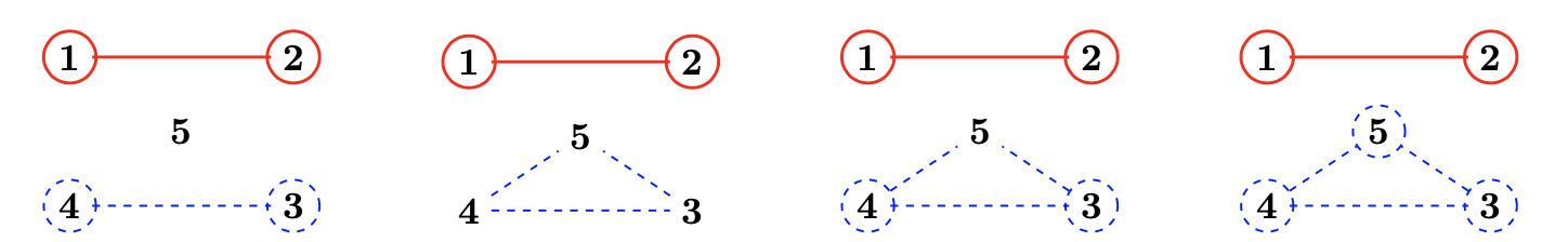
Figure 3: No bicolored vertex

There is at least one isolated edge, which is not a $zw$-edge. Let us say it is a $z$-edge. The complement has 3 bodies. There three can have one or three $w$-edges according to Rule VI.

For one $w$-edge, the attached bodies have to be $w$-circled by Rule I. This is the first diagram in Figure 3.

For three $w$-edges, the three edges form a triangle. There are three possibilities for the number of $w$-circled vertices: it is either zero, or two or three (one is not possible by Rule III.) They constitute the last three diagrams in Figure 3.

The case with zero $w$-circles is impossible. Applying Proposition 4.5 to vertex 1 and vertex 2, we see $\Lambda=\pm 1$ or $\pm\textbf{i}$. The mass constraints are

• $\Gamma_{3}+\Gamma_{4}+\Gamma_{5}=0,\Gamma_{1}+\Gamma_{2}\neq 0$, if $\Lambda=\pm 1$;

• $\Gamma_{1}\Gamma_{2}=L_{345},L=0,\Gamma_{1}+\Gamma_{2}\neq 0$, if $\Lambda=\pm\textbf{i}$.

Applying Proposition 4.3 to vertices 3, 4 and 5 we have $L_{345}=0$. This constraint is not compatible with neither one of the above two constraints. Hence, this diagram is impossible.

Hence, we could not exclude the first, the third and the last diagrams in Figure 3. There are three possible diagrams.

4.2 $C=2$

There are two cases: a $zw$-edge exists or not.

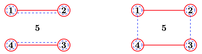
Figure 4: $C=2$

If it is present, it is isolated. Let us say, vertex 1 and vertex 2 are connected by one $zw$-edge. Among vertices 3, 4, and 5, there exist both $z$ and $w$-circle. If none of the three vertices is $z$-circled, we have $\Gamma_{1}+\Gamma_{2}=0$ by Proposition 4.2. On the other hand, since vertices 3, 4, and 5 are not $z$-circled, they are not $z$-close to vertex 1 and vertex 2 . Then Proposition 4.1 implies that $\Gamma_{1}+\Gamma_{2}\neq 0$. This is a contradiction.

Then Rule I implies that there is at least one $z$-stroke and one $w$-stroke among the cluster of vertices 3, 4, and 5. There are two possibilities: whether there is another $zw$-edge or not.

If another $zw$-edge is present, then it is again isolated. This is the first diagram in Figure 4.

If another $zw$-edge is not present, there is at least one edge in both color. By the circling method, the adjacent vertex is $z$- and $w$-circled. By the Estimate, the $z$-edge implies the two attached vertices are $w$-close. Then the two ends are both $w$-circled by Rule II. Thus, all three vertices are $z$- and $w$-circled. Then there is more strokes in the diagram. This is a contradiction.

If there is no $zw$-edge, there are adjacent $z$-edges and $w$-edges. From any such adjacency there is no other edge. Suppose that vertex 1 connects with vertex 4 by $w$-edges and connects with 2 by $z$-edges. The circling method implies that 1 is $z$- and $w$-circled, 2 is $w$-circled and 4 is $z$-circled. The color of 2 and 4 forces the color of edges from the circle. If the two edgers go to the same vertex, we get the diagram corresponding to Roberts’ continuum at infinity, shown as the second in Figure 4.

If the two edgers go to the different vertices, the circling method demands a cycle with alternating colors, which is impossible since we have only five edges.

Hence, there are two possible diagrams, see Figure 4.

4.3 $C=3$

Consider a bicolored vertex with three strokes. It is Y-shaped or connects a single stroke to a $zw$-edge.

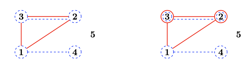
Figure 5: $C=3$

We start with the Y-shaped case. Let us say vertex 1 connects with vertex 2 and vertex 3 by $z$-edges, and connects with vertex 4 by a $w$-edge. There is a $z_{23}$-stroke by Rule VI. The circling method implies that the vertices 1, 2 and vertex 3 are all $w$-circled, see Figure 5. Then there is $w$-stroke emanating from 2 and vertex 3. The $w$-stroke may go to vertex 4, vertex 5, or it is a $w_{23}$-stroke.

If one $w$-stroke goes from vertex 2 to vertex 4, then there is extra $w_{12}$-stroke by Rule VI, which contradict with $C=3$. If all two $w$-strokes go to vertex 5, then Rule VI implies the existence of $w_{23}$-stroke. This is again a contradiction with $C=3$.

If the $w$-strokes emanating from 2 and vertex 3 is just $w_{23}$-stroke. Then we have an $zw$-edge between 2, and 3. Then it is not necessary to discuss the $zw$-edge case. Then we consider the vertex 5 . It is connected with the previous four vertices or isolated.

If the diagram is connected, vertex 5 can only connects with vertex 4 by a $z$-edge (other cases is not possible by Rule VI). Then the circling method implies that vertex 5 is $w$-circled. Then there is $w$-stroke emanating from 5. This is a contradiction.

If vertex 5 is isolated. Then the circling method implies that all vertices except vertex 5 are $w$-circled. Only 2 and vertex 3 can be $z$-circled, and they are both $z$-circled or both not $z$-circled by Rule IV, see Figure 5.

If both vertex 2 and vertex 3 are not $z$-circled, then we have $\Gamma_{2}+\Gamma_{3}=0$ and $L_{123}=0$ by Proposition 4.2 and Proposition 4.3. This is a contradiction since

$$L_{123}=\Gamma_{1}(\Gamma_{2}+\Gamma_{3})+\Gamma_{2}\Gamma_{3}.$$

If both vertex 2 and vertex 3 are $z$-circled, then Proposition 4.2 implies that $\Gamma_{2}+\Gamma_{3}=0$. On the other hand, Proposition 4.1 implies that $\Gamma_{2}+\Gamma_{3}\neq 0$. This is a contradiction.

Thus, the two diagrams in Figure 5 are both excluded. we have no possible diagram.

4.4 $C=4$

There are five cases: two $zw$-edges, only one $zw$-edge and one edge of each color, only one $zw$-edge and two edge of the same color, one $z$-edge and three $w$-edges, or two edges of each color emanating from the same vertex.

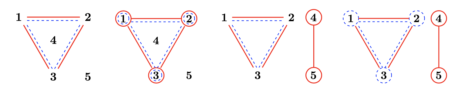
Figure 6: $C=4$, two $zw$-edges

4.4.1

Suppose that there are two $zw$-edges emanating from, e.g., vertex 1 as on the first diagram in Figure 6.

We get a fully $zw$-edged triangle by Rule VI. This triangle is isolated since $C=4$. Since vertices 1, 2, and 3 are $z$-close and $w$-close, if one of them is circled in some color, all of them will be circled in the same color. Thus, the first three vertices may be all $z$-circled, all $z$-and $w$-circled, or all not circled.

If vertices 1, 2, and 3 are $z$-circled but not $w$-circled, we have $\Gamma_{1}+\Gamma_{2}+\Gamma_{3}=0$ and $L_{123}=0$ by Proposition 4.2 and Proposition 4.3. This is a contradiction since $(\Gamma_{1}+\Gamma_{2}+\Gamma_{3})^{2}-2L_{123}\neq 0$. Then the first three vertices can only be all $z$-and $w$-circled, or all not circled.

The other two vertices can be disconnected, connected by one , e.g., $z$-edge, or by one $zw$-edge.

If vertex 4 and vertex 5 are connected by one $zw$-edge, then there are two possibilities: whether the first three vertices are all $z$-and $w$-circled, or all not circled. In the first case, we have $\Gamma_{1}+\Gamma_{2}+\Gamma_{3}=0$ and $\Gamma_{4}+\Gamma_{5}=0$ by Proposition 4.2. Then the total vorticity is zero, which contradicts with our assumption on the vorticity. In the second case, we have $\Gamma_{4}+\Gamma_{5}=0$ by Proposition 4.2. On the other hand, since vertices 1, 2, and 3 are not $z$-circled, they are not $z$-close to vertex 4 and vertex 5 . Then Proposition 4.1 implies that $\Gamma_{4}+\Gamma_{5}\neq 0$. This is a contradiction.

Then we have the four possibilities, see Figure 6. The third diagram is impossible. The argument is similar to that corresponding to the second diagram in Figure 3.

4.4.2

Suppose that there are one $zw$-edges and one edge of each color emanating from vertex 1, as in the first digram of Figure 7. We have a “butterfly diagram” by Rule VI. Note that no more strokes can emanating from vertex 1 and vertex 4 since $C=4$. If there are more strokes from vertex 2, it can not goes to vertex 3, since it implies one more stroke emanating from vertex 1. Similarly, there is no $z_{35}$-stroke or $w_{25}$-stroke. Then between vertex 5 and the first four vertices, there can have no edge, one $z_{25}$-stroke, or one $z_{25}$-stroke and one $w_{35}$-stroke.

For the disconnected diagram, vertex 1 and vertex 4 can not be circled. Otherwise, the circling method implies either vertex 2 is be $z$-circled or 3 is $w$-circled, there should be stroke emanating from vertex 2 or vertex 3 . This is a contradiction. Then vertex 2 can not be circled, otherwise, vertex 3 is of the same color by Rule IV. This is a contradiction. Hence, there is no circle in the diagram and this is the first diagram in Figure 7.

If there is only $z_{25}$-stroke, then the circling method implies that vertices 1, 2, 4, and 5 are $z$-circled. Note that vertex 3 and vertex 5 can not be $w$-circled, otherwise there are extra $w$-strokes. Then vertices 1, 2, and 4 are not $w$-circled by the circling method. Note that vertex 3 must be $z$-circled, otherwise, we have $L_{124}=0$ and $\Gamma_{1}+\Gamma_{4}=0$. This is a contradiction. Then we have the second diagram in Figure 7.

If there are $z_{25}$-stroke and $w_{35}$-stroke. Then vertex 5 is $z$-and $w$-circled. By the circling method, all vertices are $z$-and $w$-circled. This the third diagram in Figure 7.

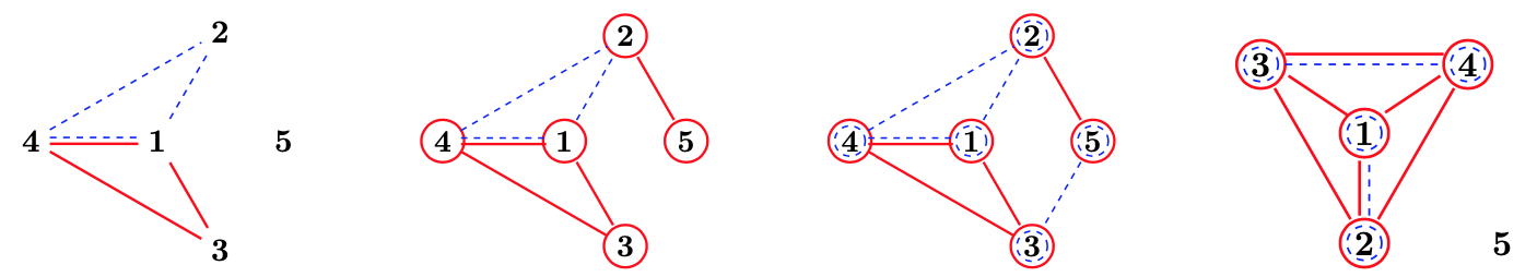
Figure 7: $C=4$, one $zw$-edges

4.4.3

Suppose that there are one $zw$-edges and two $z$-edges emanating from vertex 1, as in the fourth diagram in Figure 7. Then there are $z_{23}$-stroke, $z_{24}$-stroke and $z_{34}$-stroke by Rule VI. Note that vertex 1 is $z$-circled, then the circling method implies all vertices except possibly vertex 5 are $w$-circled. Then there is $w$-stroke emanating from 3 and vertex 4. The $w$-stroke may go to vertex 5, or it is a $w_{34}$-stroke.

If all two $w$-strokes go to vertex 5, then Rule VI implies the existence of $w_{34}$-stroke, which contradicts with $C=4$. Then the $w$-strokes from 3 and vertex 4 is $w_{34}$-stroke, and vertex 5 is disconnected.

Consider the circling the the diagram. We have three different cases: all vertices are not $z$-circled, only two of the first four vertices, say, vertex 1 and vertex 2 are $z$-circled, or all the first four vertices are $z$-circled.

If none of the first four vertices is $z$-circled, then we have $\Gamma_{1234}=0$ and $L_{1234}=0$ by Proposition 4.2 and Proposition 4.4. This is a contradiction.

If only vertex 1 and vertex 2 are $z$-circled, we have $\Gamma_{1}+\Gamma_{2}=0$ by Proposition 4.2. On the other hand, since vertices 3, 4, and 5 are not $z$-circled, they are not $z$-close to vertex 1 and vertex 2 . Then Proposition 4.1 implies that $\Gamma_{1}+\Gamma_{2}\neq 0$. This is a contradiction.

Hence, all the first four vertices are $z$-circled. This gives the fourth diagram in Figure 7.

4.4.4

Suppose that from vertex 1 there are three $w$-edges go to vertex 2, vertex 3 and vertex 4 respectively and one $z$-edges goes to vertex 5 . There is a $w$-stroke between any pair of $\{\textbf{1, 2, 3, 4}\}$ by Rule VI, and the four vertices are all $z$-circled.

Then there are $z$-strokes emanating from vertex 2, vertex 3 and vertex 4 . None of them can go to vertex 5 by Rule VI. Then there are $z_{23}$-, $z_{24}$- and $z_{34}$-strokes. This contradict with $C=4$. Hence, there is no possible diagram in this case.

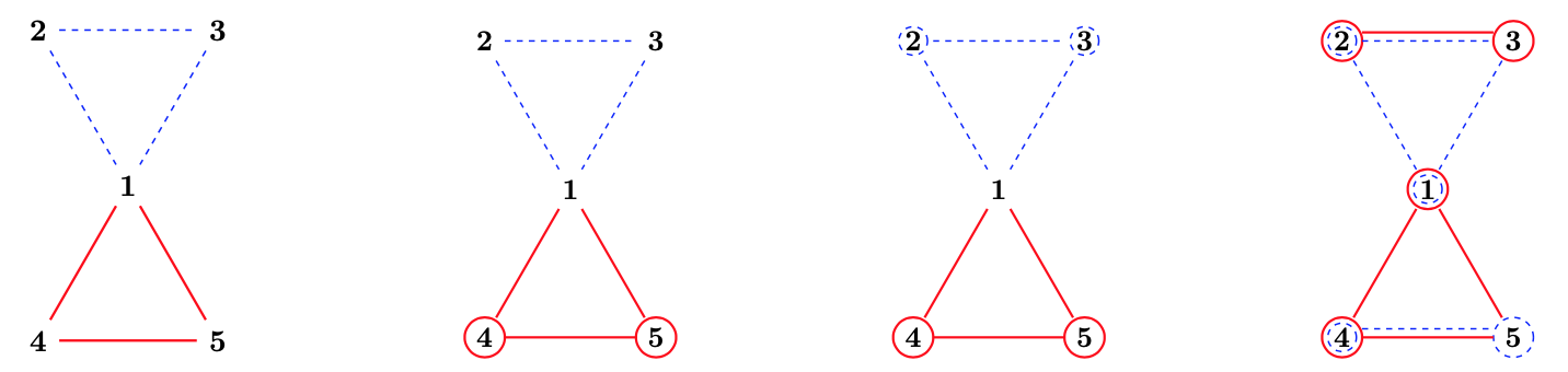
Figure 8: $C=4$, no $zw$-edges

4.4.5

Suppose that there are two $w$-edges and two $z$-edges emanating from vertex 1, with numeration as in the first digram of Figure 8. By Rule VI, there is $w_{23}$- and $z_{45}$-stroke. Thus, we have two attached triangles. By Rule VI, if there is more stroke, it must be $z_{23}$- and/or $w_{45}$-stroke.

Case I: If there is no more stroke, vertex 2 and vertex 3 can only be $w$-circled, and vertex 4 and vertex 5 can only be $z$-circled. Then vertex 1 can not be circled, otherwise, the circling method would lead to contradiction. Then we have the first three diagrams in Figure 8.

Case II: If there is only $z_{23}$-stroke, the circling method implies vertex 1, vertex 2 and vertex 3 are $z$-circled. Note that only vertex 2 and vertex 3 can be $w$-circled. There are two possibilities: whether vertex 2 and vertex 3 are both $w$-circled or both not $w$-circled.

If vertex 2 and vertex 3 are both $w$-circled, we have $\Gamma_{2}+\Gamma_{3}=0$ by Proposition 4.2. On the other hand, since vertices 1, 4, and 5 are not $w$-circled, they are not $w$-close to vertex 2 and vertex 3 . Then Proposition 4.1 implies that $\Gamma_{2}+\Gamma_{3}\neq 0$. This is a contradiction.

If vertex 2 and vertex 3 are both not $w$-circled, we have $\Gamma_{2}+\Gamma_{3}=0$ and $L_{123}=0$ by Proposition 4.2 and Proposition 4.3. This is a contradiction. Hence there is no possible diagram in this case.

Case III: If there are $z_{23}$- and $w_{45}$-strokes, the circling method implies vertex 2 and vertex 3 are $z$-circled, vertex 4 and vertex 5 are $w$-circled, and vertex 1 is $z$- and $w$-circled. Consider the circling of vertex 2 and vertex 3, there are three possibilities: there are zero, one, or two $w$-circles.

If both vertex 2 and vertex 3 are not $w$-circled, then the upper triangle, which is isolated in $w$-diagram, has only one $w$-circle, namely, vertex 1. This is a contradiction by Rule IV.

If both vertex 2 and vertex 3 are $w$-circled, then we have $\Gamma_{2}+\Gamma_{3}=0$ by Proposition 4.2. Consider the upper triangle in $w$-diagram. We have

$$\Gamma_{1}w_{1}+\Gamma_{2}w_{2}+\Gamma_{3}w_{3}=\Gamma_{1}w_{1}+(\Gamma_{2}+\Gamma_{3})w_{2}\approx\Gamma_{1}w_{1}<\epsilon^{-2}.$$

Then we have $\Gamma_{1}=0$, which is a contradiction.

Repeat the argument for vertex 4 and vertex 5. Hence, the only possible diagram in this case is that only one of vertex 2 and vertex 3 is $w$-circled and only one of vertex 4 and vertex 5 is $z$-circled. This is the last diagram in Figure 8.

However, this diagram is impossible. Vertex 2 and vertex 3 are $w$-close, so they should be both $w$-circled by Rule II.

In summary, among the twelve diagrams in Figure 6, 7 and 8, we have excluded the third one in Figure 6 and the fourth one in Figure 8. We have ten possible diagrams.

4.5 $C=5$

There are three cases: two $zw$-edges, one $zw$-edge with one $z$-edge and two $w$-edges, one $zw$-edge with three $z$-edges.

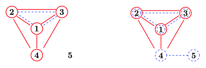
Figure 9: $C=5$, two $zw$-edges

4.5.1

Suppose that there are two $zw$-edges and one $z$-edges emanating from vertex 1, with numeration as in the first digram of Figure 9. Rule VI implies the existence of $zw_{23}$-, $z_{24}$- and $z_{34}$-edges. Then vertex 5 can be either disconnected or connects with vertex 4 by one $w$-edge, otherwise, it would contradicts with $C=5$.

For the disconnected diagram, note that any of the connected four vertices can not be $w$-circled. Otherwise the circling method implies vertex 4 is $w$-circled, which is a contradiction. There are three cases: none of the vertices are circled, all four vertices except vertex 4 are $z$-circled, or all four vertices are $z$-circled.

If none of the vertices are circled, by Proposition 4.3 we have $L_{123}$ since vertices 1, 2, and 3 form a triangle with no $w$-circled attached. Similarly, we have $L_{1234}=0$ by Proposition 4.4. This is a contradiction since

$$L_{1234}=L_{123}+\Gamma_{4}(\Gamma_{1}+\Gamma_{2}+\Gamma_{3}),\ (\Gamma_{1}+\Gamma_{2}+\Gamma_{3})^{2}-2L_{123}\neq 0.$$

If only vertices 1, 2, and 3 are $z$-circled, we also have $L_{123}$. By Proposition 4.2, we have $\Gamma_{1}+\Gamma_{2}+\Gamma_{3}=0$. This is a contradiction.

Hence, we have only one possible diagram for the disconnected diagram, and it is the first in Figure 9.

For the connected diagram with $w_{45}$-edge, the circling method implies that all vertices are $w$-circled. Note that vertex 4 and vertex 5 can not be $z$-circled. Then we have two cases: all of the five vertices are not $z$-circled, or vertices 1, 2, and 3 are $z$-circled.

If all of the five vertices are not $z$-circled, we have $\Gamma_{1}+\Gamma_{2}+\Gamma_{3}=0$ by Proposition 4.2 and $L_{1234}=0$ by Proposition 4.4. This is a contradiction.

Hence, we have only one possible diagram for the connected diagram, and it is the second in Figure 9.

4.5.2

Suppose that there are one $zw$-edge, one $z$-edge, and two $w$-edges emanating from vertex 1, with numeration as in the first digram of Figure 10. Rule VI implies that vertices 1, 2, 3, and 4 are fully $w$-stroked, and that vertices 1, 3, and 5 are fully $z$-stroked. There is no more stroke emanating from vertices 1, 3, and 5, since that would contradicts with $C=5$. There are two cases, $z_{24}$-stroke is present or not.

If it is not present, vertex 2 and vertex 4 can only be $w$-circled, and vertex 5 can only be $z$-circled. Then vertex 1 and vertex 3 can not be circled, otherwise, the circling method would lead to contradiction. Then we have the first two diagrams in Figure 10 by Rule IV.

If $z_{24}$-stroke is present, then vertices 1, 2, 3, and 4 are all $z$-circled. Vertex 1 and vertex 3 can not be $w$-circled, which would lead to vertex 5 also $w$-circled and a contradiction. Vertex 2 and vertex 4 are $w$-close, so they are both $w$-circled or both not $w$-circled. If they are both $w$-circled, then Proposition 4.2 implies that $\Gamma_{2}+\Gamma_{4}=0$. On the other hand, Proposition 4.1 implies that $\Gamma_{2}+\Gamma_{4}\neq 0$. This is a contradiction.

Then according to whether vertex 5 is $z$-circled or not, we have two cases, which are the last two diagrams in Figure 10.

The third diagram in Figure 10 is impossible. We would have $L_{1234}=0$ and $\sum_{j=1}^{4}\Gamma_{j}=0$ by Proposition 4.4 and Proposition 4.2. Hence, we have only one possible diagram if $z_{24}$-stroke is present, and it is the last diagram in Figure 10.

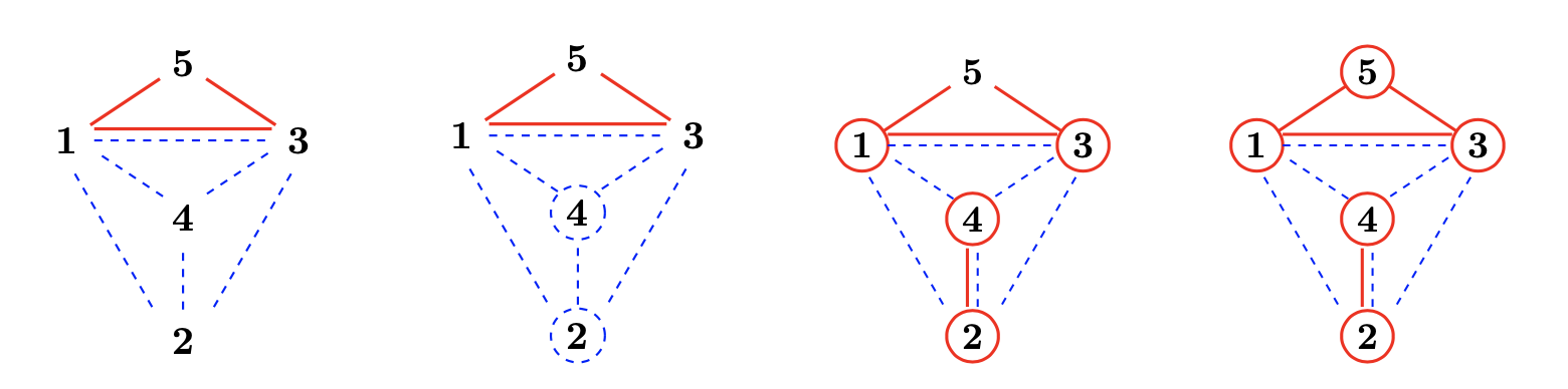
Figure 10: $C=5$, one $zw$-edges

4.5.3

Suppose that there are one $zw$-edge and three $w$-edges emanating from vertex 1 . Let us say, the $zw$-edge goes to vertex 2 and the other edges go to the other three vertices. Rule VI implies that vertices 1, 2, 3, 4, 5 are fully $w$-stroked. The circling method implies that all vertices are $z$-circled. Then there are $z$-strokes emanating from vertices 3, 4, and 5. Since $C=5$ at vertex 1 and vertex 2, the $z$-strokes from vertices 3, 4, and 5 must go to vertices 3, 4, and 5. By Rule VI, they form a triangle of $z$-strokes. This is a contradiction with $C=5$.

In summary, among the six diagrams in Figure 9 and 10, we have excluded the third one in Figure 10. We have five possible diagrams.

4.6 $C=6$

There are three cases: three $zw$-edges, two $zw$-edge with one edge in each color, two $zw$-edge with two $z$-edge.

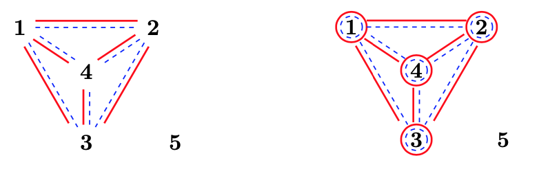
Figure 11: $C=6$, three $zw$-edges

4.6.1

Suppose that there are three $zw$-edges emanating from vertex 1, with numeration as in the first digram of Figure 11. Rule VI implies that the vertices 1, 2, 3, and 4 are fully $zw$-edged. Then vertex 5 must be disconnected since $C=6$. The first four vertices can be circled in the same way by the circling method.

If all of the first four vertices are $z$-circled but not $w$-circled, then we would have we would have $L_{1234}=0$ and $\sum_{j=1}^{4}\Gamma_{j}=0$ by Proposition 4.4 and Proposition 4.2. This is one contradiction.

Hence, we have two possible diagrams if there are three $zw$-edges, which are the two diagrams in Figure 11.

4.6.2

Suppose that there are two $zw$-edges and two $z$-edges emanating from vertex 1, with numeration as in the first digram of Figure 12. Rule VI implies the existence of $z_{25}$-, $z_{35}$-, $z_{24}$-, $z_{45}$- and $z_{34}$-strokes, and that the vertices 1, 2, and 3 are fully $zw$-edged. If there is more stroke, it must be $w_{45}$-stroke since $C=6$.

If there is no more stroke, then the vertices can only be $z$-circled. There are two cases, either vertices 1, 2, and 3 are $z$-circled or not.

If vertices 1, 2, and 3 are $z$-circled, then either vertex 4 or vertex 5 must also be $z$-circled. Otherwise, we have $\Gamma_{1}+\Gamma_{2}+\Gamma_{3}=0$ and $L_{123}=0$ by Proposition 4.4 and Proposition 4.2. This is one contradiction. Then we have the first two diagrams in Figure 12.

If vertices 1, 2, and 3 are not $z$-circled, then vertex 4 and vertex 5 are both $z$-circled or both not $z$-circled. Then we have the second two diagrams in Figure 12.

If $w_{45}$-stroke is present, then the circling method implies that all vertices are $w$-circled. Then we have $\Gamma_{4}+\Gamma_{5}=0$ and $\Gamma_{1}+\Gamma_{2}+\Gamma_{3}=0$ by Proposition 4.2, which contradicts with our assumption that the total vorticity is not zero.

4.6.3

Suppose that there are two $zw$-edges and one edge of each color emanating from vertex 1, with numeration as in the first digram of Figure 13. Rule VI implies the existence of $w_{25}$-, $w_{35}$-, $z_{24}$-, and $z_{34}$-strokes, and that the vertices 1, 2, and 3 are fully $zw$-edged. If there is more stroke, it must be $w_{45}$-stroke, but it would lead to extra stroke emanating from vertex 1, which contradicts with $C=6$.

Vertex 4 can only be $w$-circled, and vertex 4 can only be $z$-circled. Then vertices 1, 2 and 3 can not be circled, otherwise, the circling method would lead to contradiction. Then we have the diagram in Figure 13 by Rule IV.

In summary, we have seven possible diagrams, see Figure 11, 12, and 13.

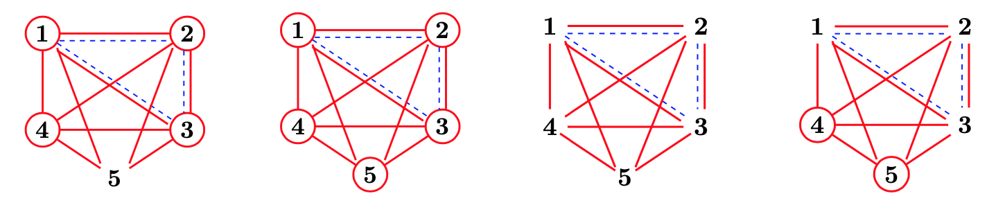
Figure 12: $C=6$, two $zw$-edges, case 1

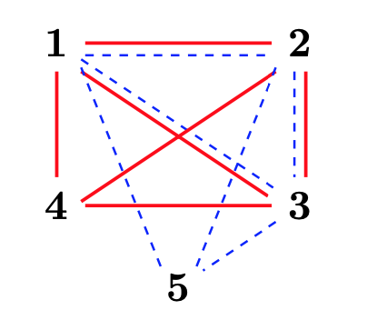
Figure 13: $C=6$, two $zw$-edges, case 2

4.7 $C=7$

Suppose that there are three $zw$-edges and one $z$-edge emanating from vertex 1, with numeration as in the digram of Figure 14. Rule VI implies that the vertices 1, 2, 3, and 4 are fully $zw$-edged and that vertex 5 connects with the first four vertices by one $z$-edge. There is no more stroke since $C=7$. If any vertex is $w$-circled, all are $w$-circled, which would lead to $w$-stroke emanating from vertex 5 . This is a contradiction. There are two cases, either vertex 1 is $z$-circled or not.

If vertex 1 is not $z$-circled, then none of the vertices is $z$-colored by the circling method. Then $L_{1234}=0$ by Proposition 4.4. By the estimate, we have

$$r_{ij}\approx\epsilon^{2},\ 1\leq i<j\leq 4,\ r_{5k}^{4}=w_{5k}z_{5k}<\epsilon^{2}\epsilon^{-2}<1.$$

Then $S=0$ on the continuum corresponding to this diagram. Then we have $\Gamma=0$ or $L=0$ by Proposition 2.2. The first case contradicts with our assumption of the total vorticity. The second case leads to $\Gamma_{5}=0$ since

$$L=L_{1234}+\Gamma_{5}(\sum_{j=1}^{4}\Gamma_{j}),\ (\sum_{j=1}^{4}\Gamma_{j})^{2}-2L_{1234}\neq 0.$$

If vertex 1 is $z$-circled, then vertices 1, 2, 3, and 4 are all $z$-circled. Then vertex 5 can be $z$-circled or not.

If vertex 5 is not $z$-circled, we have $L_{1234}=0$ and $\sum_{j=1}^{4}\Gamma_{j}=0$ by Proposition 4.4 and Proposition 4.2. This is a contradiction.

Hence, we only have one diagram in the case of $C=7$, as in Figure 14.

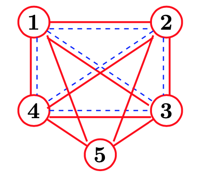
Figure 14: $C=7$

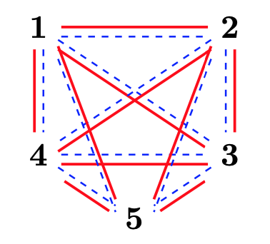
Figure 15: $C=8$

4.8 $C=8$

Suppose that there are four $zw$-edges emanating from vertex 1 . Rule VI implies that the vertices 1, 2, 3, 4, 5 are fully $zw$-edged. Since all vertices are both $z$-close and $w$-close, any circle would implies that the total vorticity is zero, which contradicts with our assumption on the total vorticity.

Hence, we only have one diagram in the case of $C=8$, as in Figure 15.

To summarize, we have excluded the second diagram in Figure 3, the two diagrams in Figure 5, the third diagram in Figure 6, the fourth diagram in Figure 8, the third diagram in Figure 10. The conclusion of the section is that any singular sequence should converge to one of the twenty-nine diagrams in Figure 16.

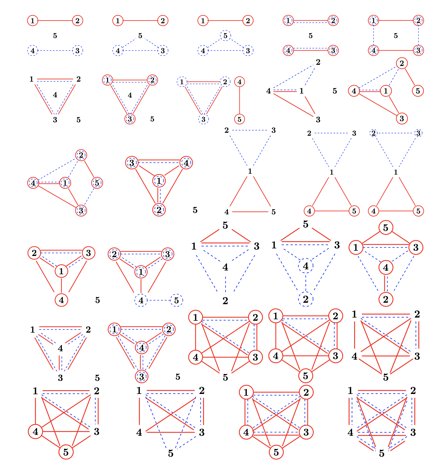
Figure 16: The twenty-nine 5-vortex diagrams

5 The twenty-nine remaining 5-vortex diagrams

In the previous process of eliminating 5-body diagrams, we could not eliminate the twenty-nine diagrams in Figure 16. Some singular sequence could still exist and approach any of these diagrams. These diagrams will be excluded except if the vorticities satisfy a polynomial relation. We discuss the constraints on the vorticities corresponding to each of the twenty-nine diagrams. We number 5.1 to 5.29 the discussions of the constraints on the vorticities corresponding to each of the twenty-nine diagrams from Figure 16, ordered horizontally from top left to bottom right.

$5.1$.   Applying Proposition 4.5 to vertex 1 and vertex 2, then to vertex 3 and vertex 4, we see $\Lambda=\pm 1$ or $\pm\textbf{i}$. The mass constraints are

• $\Gamma_{1}+\Gamma_{2}+\Gamma_{5}=0,\Gamma_{1}+\Gamma_{2}=\Gamma_{3}+\Gamma_{4}\neq 0$, if $\Lambda=\pm 1$;

• $\Gamma_{1}\Gamma_{2}=L_{345},\Gamma_{3}\Gamma_{4}=L_{125},L=0,\Gamma_{1}+\Gamma_{2}\neq 0,\Gamma_{3}+\Gamma_{4}\neq 0$, if $\Lambda=\pm\textbf{i}$.
  

$5.2$.  Applying Proposition 4.5 to vertex 1 and vertex 2, we see $\Lambda=\pm 1$ or $\pm\textbf{i}$. The mass constraints are

• $\Gamma_{3}+\Gamma_{4}+\Gamma_{5}=0,\Gamma_{1}+\Gamma_{2}\neq 0$, if $\Lambda=\pm 1$;

• $\Gamma_{1}\Gamma_{2}=L_{345},L=0,\Gamma_{1}+\Gamma_{2}\neq 0$, if $\Lambda=\pm\textbf{i}$.

Applying Proposition 4.6 to vertices 3, 4 and 5, we see $\Lambda=\pm 1$ or $\pm\textbf{i}$. The mass constraints are

• $\Gamma_{1}+\Gamma_{2}=\Gamma_{5},\Gamma_{3}+\Gamma_{4}\neq 0$, if $\Lambda=\pm 1$;

• $L_{345}=L_{125},L=0,\Gamma_{3}+\Gamma_{4}\neq 0$, if $\Lambda=\pm\textbf{i}$.

Hence, the mass constraints are

• $\Gamma_{3}+\Gamma_{4}+\Gamma_{5}=0,\Gamma_{1}+\Gamma_{2}=\Gamma_{5},\Gamma_{1}+\Gamma_{2}\neq 0,\Gamma_{3}+\Gamma_{4}\neq 0$, if $\Lambda=\pm 1$;

• $\Gamma_{1}\Gamma_{2}=L_{345},L=0,L_{345}=L_{125},\Gamma_{1}+\Gamma_{2}\neq 0,\Gamma_{3}+\Gamma_{4}\neq 0$, if $\Lambda=\pm\textbf{i}$.

Note the case $\Lambda=\pm\textbf{i}$ implies $\Gamma_{5}=0$, which contradicts our assumption on the masses. Thus, we have

$$\Gamma_{3}+\Gamma_{4}+\Gamma_{5}=0,\Gamma_{1}+\Gamma_{2}=\Gamma_{5},\Gamma_{1}+\Gamma_{2}\neq 0,\Gamma_{3}+\Gamma_{4}\neq 0,\ \Lambda=\pm 1$$

$5.3$.   Applying Proposition 4.5 to vertex 1 and vertex 2, we see $\Lambda=\pm 1$ or $\pm\textbf{i}$. The mass constraints are

• $\Gamma_{3}+\Gamma_{4}+\Gamma_{5}=0,\Gamma_{1}+\Gamma_{2}\neq 0$, if $\Lambda=\pm 1$;

• $\Gamma_{1}\Gamma_{2}=L_{345},L=0,\Gamma_{1}+\Gamma_{2}\neq 0$, if $\Lambda=\pm\textbf{i}$.
  

$5.4$.  Applying Proposition 4.2 to vertex 1 and vertex 2, then to vertex 3 and vertex 4, we obtain

$$\Gamma_{1}+\Gamma_{2}=0,\ \Gamma_{3}+\Gamma_{4}=0.$$

$5.5$.   Consider the isolated component $z_{12}$-edge. By Rule III, $\Gamma_{1}z_{1}+\Gamma_{2}z_{2}\prec\epsilon^{-2}$. Without loss of generality, assume $z_{1}\sim-\Gamma_{2}a\epsilon^{-2}$ and $z_{2}\sim\Gamma_{1}a\epsilon^{-2}$.Similarly, we assume $z_{3}\sim-\Gamma_{4}b\epsilon^{-2}$ and $z_{4}\sim\Gamma_{3}b\epsilon^{-2}$. Since $z_{14}\approx z_{23}\approx\epsilon^{2}$ by the estimate, we obtain

$$-\Gamma_{2}a=\Gamma_{3}b,\ \Gamma_{1}a=-\Gamma_{4}b.$$

Hence we obtain

$$\Gamma_{1}\Gamma_{3}=\Gamma_{2}\Gamma_{4}.$$

$5.6$.   Applying Proposition 4.3 to vertices 1, 2, and 3, we obtain

$$L_{123}=0.$$

$5.7,5.8$.   Applying Proposition 4.2 to vertices 1, 2, and 3, we obtain

$$\Gamma_{1}+\Gamma_{2}+\Gamma_{3}=0.$$

$5.9$.   Applying Proposition 4.3 to vertices 1, 2, and 4, then to vertices 1, 3, and 4, we obtain

$$L_{124}=L_{134}=0.$$

$5.10$.  Applying Proposition 4.3 to vertices 1, 2, and 4, we obtain

$$L_{124}=0.$$

$5.11$.  Note that

$$\Gamma_{1}z_{1}+\Gamma_{4}z_{4}\sim(\Gamma_{1}+\Gamma_{4})z_{1},\ \Gamma_{1}w_{1}+\Gamma_{4}w_{4}\sim(\Gamma_{1}+\Gamma_{4})w_{1},\ z_{2}\sim z_{1},\ w_{3}\sim w_{1}.$$

Then $\Gamma_{1}+\Gamma_{4}\neq 0$. By Rule III, we have

$$\begin{array}[]{c}(\Gamma_{1}+\Gamma_{4})w_{1}+\Gamma_{2}w_{2}\prec\epsilon^{-2},\ (\Gamma_{1}+\Gamma_{4})z_{1}+\Gamma_{3}z_{3}\prec\epsilon^{-2},\cr\Gamma_{3}w_{3}+\Gamma_{5}w_{5}\prec\epsilon^{-2},\ \Gamma_{2}z_{1}+\Gamma_{5}z_{5}\prec\epsilon^{-2}.\end{array}$$

These relations imply

$$w_{2}\sim-\frac{\Gamma_{1}+\Gamma_{4}}{\Gamma_{2}}w_{1},\ w_{5}\sim-\frac{\Gamma_{5}}{\Gamma_{3}}w_{1},\ z_{3}\sim-\frac{\Gamma_{1}+\Gamma_{4}}{\Gamma_{3}}z_{1},\ z_{5}\sim-\frac{\Gamma_{5}}{\Gamma_{2}}z_{1}.\$$

Then the relations $z_{3}\sim z_{5},w_{2}\sim w_{5}$ lead to $\Gamma_{2}(\Gamma_{1}+\Gamma_{4})=\Gamma_{3}\Gamma_{5}$ and $\Gamma_{3}(\Gamma_{1}+\Gamma_{4})=\Gamma_{2}\Gamma_{5}$. Thus, the constraints are

$$\Gamma_{2}=\Gamma_{3},\ \Gamma_{1}+\Gamma_{4}=\Gamma_{5}.$$

$5.12$.  Applying Proposition 4.2 to vertices 1 and 2, then to vertices 4 and 5, we obtain

$$\Gamma_{1}+\Gamma_{2}=0,\ \Gamma_{4}+\Gamma_{5}=0.$$

$5.13$.  Applying Proposition 4.3 to the two attached triangles respectively, we obtain

$$L_{123}=0,\ L_{145}=0.$$

$5.14$.  Applying Proposition 4.6 to vertex 4 and vertex 5, Proposition 4.3 to vertices 1, 2, and 3, we see $\Lambda=\pm 1$ or $\pm\textbf{i}$. The mass constraints are

• $\Gamma_{1}=\Gamma_{2}+\Gamma_{3},L_{123}=0,\Gamma_{4}+\Gamma_{5}\neq 0$, if $\Lambda=\pm 1$;

• $L_{145}=0,L=0,L_{123}=0,\Gamma_{4}+\Gamma_{5}\neq 0$, if $\Lambda=\pm\textbf{i}$.
  

$5.15$.  Applying Proposition 4.6 to the upper and lower triangle respectively, we see $\Lambda=\pm 1$ or $\pm\textbf{i}$. The mass constraints are

• $\Gamma_{1}=\Gamma_{4}+\Gamma_{5},\Gamma_{1}=\Gamma_{2}+\Gamma_{3},\Gamma_{2}+\Gamma_{3}\neq 0$, if $\Lambda=\pm 1$;

• $L=0,L_{145}=L_{123},\Gamma_{2}+\Gamma_{3}\neq 0,\Gamma_{4}+\Gamma_{5}\neq 0$, if $\Lambda=\pm\textbf{i}$.
  

$5.16$.  Applying Proposition 4.3 to vertices 1, 2, and 3, we see

$$L_{123}=0.$$

$5.17$.  Applying Proposition 4.2 to vertices 1, 2, and 3, we see

$$\Gamma_{1}+\Gamma_{2}+\Gamma_{3}=0.$$

$5.18$.  Applying Proposition 4.3 to vertices 1, 3 and 5, we see $L_{135}=0$. Applying Proposition 4.4 to vertices 1, 2, 3, 4, we see $L_{1234}=0$.

$5.19$.  Applying Proposition 4.3 to vertices 1, 3 and 5, we see $L_{135}=0$.

$5.20$.  Applying Proposition 4.4 to vertices 1, 2, 3, 4, we see $L_{1234}=0$. Applying Proposition 4.2 to vertex 2 and vertex 4, we see $\Gamma_{2}+\Gamma_{4}=0$.

$5.21$.  Applying Proposition 4.4 to vertices 1, 2, 3, 4, we see $L_{1234}=0$.

$5.22$.  Applying Proposition 4.2 to vertices 1, 2, 3, 4, we see $\Gamma_{1}+\Gamma_{2}+\Gamma_{3}+\Gamma_{4}=0$.

$5.23,5.24,5.25\ {\rm and}\ 5.26$.  Applying Proposition 4.3 to vertices 1, 2, and 3, we see $L_{123}=0$.

$5.27$.  Applying Proposition 4.4 to vertices 1, 2, 3, and 4, we see $L_{1234}=0$. Applying Proposition 4.4 to vertices 1, 2, 3, 5, we see $L_{1235}=0$.

$5.28$.  Applying Proposition 4.4 to vertices 1, 2, 3, and 4, we see $L_{1234}=0$.

$5.29$.  Note that $z_{kl}\approx\epsilon^{2}$ and $w_{kl}\approx\epsilon^{2}$ for $1\leq k<l\leq 5$. Then we have $S=0$ on the continuum corresponding to this diagram. Then we have $\Gamma=0$ or $L=0$ by Proposition 2.2.

Remark 5.1

A 5-tuple of vorticities with some equal masses easily falls in the exceptional set. This is consistent with Roberts’ example of continuum in Section 2. The masses are $(2,2,2,2,-1)$, which satisfy the constraints corresponding to 5.5 and 5.6.

6 Proofs

Proof 3 (Theorem 1.1)

Suppose that there are infinitely many solutions of system (2.12) in the complex domain. At least one the squared distance $r^{2}_{kl}$, say $r_{12}^{2}$, should take infinitely many values. Lemma 2.1 implies that $r_{12}^{2}=z_{12}w_{12}$ is dominating. There is a sequence of normalized central configurations such that $r_{12}^{2}\to 0$. Then $\mathcal{Z}$ or $\mathcal{W}$ is unbounded on this sequence. We extract a singular sequence, which must correspond to one of the twenty-nine diagrams found in Section 4, or the total vorticity is zero. In either case, some explicit polynomials on the five vorticities must be satisfied.

The existence of infinitely many central configurations remains possible for vorticities satisfying some explicit polynomial relations. However, we confirm the finiteness under the following restrictions of Theorem 1.2, namely,

$$\sum_{j\in J}\Gamma_{j}\neq 0,\ \sum_{j,k\in J,j\neq k}\Gamma_{j}\Gamma_{k}\neq 0,{\rm\ where}\ J\ {\rm is\ a\ nonempty\ subset\ of\ }\{1,2,3,4,5\}.$$

Under the above restriction, a singular sequence can only approach one of the three diagrams in Figure 17, numbered from left to right. Let us first estimate the distances and the $4$-product $p_{jn}=r_{jn}^{2}r_{km}^{2}r_{ml}^{2}r_{lk}^{2}$ for each diagram.

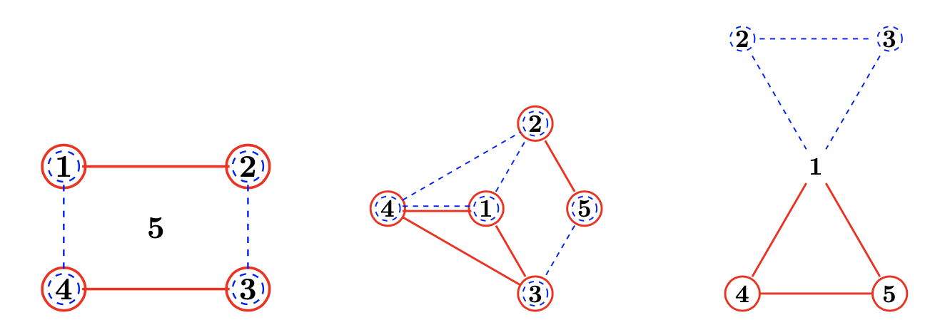
Figure 17: The three 5-vortex diagrams

The quadrilateral diagram

Consider $r_{12}^{2}=z_{12}w_{12}$. Since $Z_{12}$ is of maximal order, $w_{12}\approx\epsilon^{2}$. Since

$$\Gamma_{1}z_{1}+\Gamma_{2}z_{2}=(\Gamma_{1}+\Gamma_{2})z_{1}+\Gamma_{2}z_{12}\prec\epsilon^{-2},\ \Gamma_{1}+\Gamma_{2}\neq 0,$$

the edge $z_{12}$ is maximal. Then we have $r_{12}^{2}\approx 1$. Similarly, $w_{23},z_{34},w_{14}$ are maximal, and the side-lengths are of order $1$.

Consider the diagonals. We have $z_{24}=z_{23}+z_{34}\approx\epsilon^{-2}$ since $z_{34}$ is maximal and $z_{23}\approx\epsilon^{2}$. Similarly, $w_{24}\approx\epsilon^{-2}$. Then we have $r_{24}^{2}\approx\epsilon^{-4}$. The other diagonal have the same order. It is easy to see that squared distance from the isolated vertex 5 to other vertices are of order $\epsilon^{-4}$.

Among the ten mutual squared distances, four of them are of order $1$ and six of them are of order $\epsilon^{-4}$. We conclude that the $4$-product $p_{jn}\to\infty$ along corresponding singular sequences, for any $1\leq j<n\leq 5$.

The kite diagram

Vertex 1 and vertex 4 are close in both $z$ and $w$-coordinates. Similar to the first diagram, all strokes except $z_{14},w_{14}$ are maximal. Then the corresponding squared distances are of order $1$, and the pairs of vertices without edges correspond to squared distances of order $\epsilon^{-4}$, $r_{14}^{2}\approx\epsilon^{4}$. It is easy to see that $p_{25}$ and $p_{35}$ are of order $\epsilon^{4}$, $p_{14}$ is of order $1$, and the remaining seven $4$-product $p_{jn}$’s are of order $\epsilon^{-4}$ or $\epsilon^{-8}$, along corresponding singular sequences, for any $1\leq j<n\leq 5$. Then the product of any five $4$-products would not go to zero.

The two attached triangles

All strokes are maximal. Then the corresponding squared distances are of order $1$, and the pairs of vertices without edges correspond to squared distances of order $\epsilon^{-4}$. We conclude that the $4$-product $p_{jn}\to\infty$ along corresponding singular sequences, for any $1\leq j<n\leq 5$.

Proof 4 (Theorem 1.2)

Suppose that there are infinitely many solutions of system (2.12) in the complex domain. Repeat the argument in the proof of Theorem 1.1. We suppose that $r_{12}^{2}$ is dominating. Push it to zero. Obviously, we are in the second diagram. Then the product $p_{41}p_{42}p_{43}p_{45}p_{23}$ goes to infinity, thus is dominating by Lemma 2.1. Push the product to zero and extract a singular sequence. However, the singular sequence would correspond to none of the three diagrams. This is a contradiction.

References

- [1] Alain Albouy and Vadim Kaloshin. Finiteness of central configurations of five bodies in the plane. Annals of Mathematics, 176(1):535–588, 2012.
- [2] H. Aref. Motion of three vortices. The Physics of Fluids, 22(3):393–400, 1979.
- [3] H. Aref, P. K. Newton, M. A. Stremler, T. Tokieda, and D. L Vainchtein. Vortex crystals. Advances in applied Mechanics, 39:2–81, 2003.
- [4] W. Gröbli. Specielle Probleme über die Bewegung geradliniger paralleler Wirbelfäden, volume 8. Druck von Zürcher und Furrer, 1877.
- [5] M. Hampton and R. Moeckel. Finiteness of stationary configurations of the four-vortex problem. Transactions of the American Mathematical Society, 361(3):1317–1332, 2009.
- [6] H. Helmholtz. Über integrale der hydrodynamischen gleichungen, welche den wirbelbewegungen entsprechen. Journal für die reine und angewandte Mathematik, 1858(55):25–55, 1858.
- [7] D. Mumford. Algebraic geometry I: complex projective varieties. Springer Science & Business Media, 1995.
- [8] E. A. Novikov. Dynamics and statistics of a system of vortices. Zh. Eksp. Teor. Fiz, 68(1868-188):2, 1975.
- [9] E. A. Novikov and Yu. B. Sedov. Vortex collapse. Zhurnal Eksperimentalnoi i Teoreticheskoi Fiziki, 77:588–597, 1979.
- [10] K. A. O’Neil. Stationary configurations of point vortices. Transactions of the American Mathematical Society, 302(2):383–425, 1987.
- [11] K. A. O’Neil. Relative equilibrium and collapse configurations of four point vortices. Regular and Chaotic Dynamics, 12(2):117–126, 2007.
- [12] G. E. Roberts. A continuum of relative equilibria in the five-body problem. Physica D: Nonlinear Phenomena, 127(3-4):141–145, 1999.
- [13] J. L. Synge. On the motion of three vortices. Canadian Journal of Mathematics, 1(3):257–270, 1949.
- [14] Xiang Yu. Finiteness of stationary configurations of the planar four-vortex problem. arXiv preprint arXiv:2103.06037, 2021.