Current distributions by moving vortices in superconductors

Abstract

We take account of normal currents that emerge when vortices move. Moving Abrikosov vortices in the bulk and Pearl vortices in thin films are considered. Velocity dependent distributions of both normal and persistent currents are studied in the frame of time-dependent London equations. In thin films near the Pearl vortex core, these distributions are intriguing in particular.

I Introduction

It has been shown recently that moving vortex-like topological defects in, e.g., neutral superfluids or liquid crystals differ from their static versions [1]. This is also the case in superconductors within the Time Dependent London theory (TDL) which takes into account normal currents, a necessary consequence of moving vortex magnetic structure [2, 3, 4].

The London equations were employed for a long time to describe static or nearly static vortices out of their cores [5, 6]. The equations are linear, express the basic Meissner effect, and can be used at any temperature for problems where the cores are irrelevant. As far as their current distributions are concerned, moving vortices are commonly considered the same as static displaced as a whole.

As shown in [4], the magnetic flux carried by moving vortex is equal to the flux quantum, but is redistributed so that the part of it in front of the vortex is depleted whereas the part behind it is enhanced. This redistribution is caused by the normal currents resulting from the electric field induced by the moving non-uniform magnetic structure.

In this paper, analytic solutions are given for the field and current distributions of Abrikosov vortices moving in the bulk. It is shown that despite the anisotropic distribution of normal currents, the “topology” of supercurrents in the vicinity of the vortex core remains close to the static case with nearly cylindrical symmetry. This suggests that distortions of the vortex core shape in the bulk are weak.

The case of Pearl vortices moving in thin films is quite different. For one, the sheet currents $\bm{g}$ in the film are related to the tangential field components $h_{x,y}$, rather than to $h_{z}$ of the vortex in the bulk. In other words, they are determined by the stray field in the free space out of the film and, as a result, decay as a power law with the distance $r$ from the vortex core as compared to the exponential decay in the bulk. Besides, as $r\to 0$, the field $h_{z}\sim 1/r$, i.e. faster than $h_{z}\sim\ln(\lambda/r)$ in the bulk. Moreover, the sheet currents diverge as $1/r^{2}$ instead of bulk’s $1/r$. For any in-plane anisotropy, the supercurrents increase as $r\to 0$ leads to a situation in which the depairing value is reached at different distances for different directions that may lead to deviations of the vortex core shape from a circle of isotropic case. In particular, vortex motion is a source of such anisotropy, the subject of this work. We find the distribution of supercurrent values near the core of moving vortices is quite unconventional, see Figs. 10 and LABEL:f11.

The time-dependent London equations are employed in this paper. The equations are linear and contain the first derivative with respect to time, that makes them in a sense similar to the well-studied diffusion equation. As in diffusion case, we employ the Fourier transform in solving for fields and currents. To get results in real space, one has to calculate integrals over $k_{x},k_{y}$ of the Fourier space from $-\infty$ to $\infty$, a heavy numerical procedure. We offer a way to transform the double integrals over $\bm{k}$ to single integrals from $0$ to $\infty$ which are easily evaluated numerically.

In time dependent situations, the current consists, in general, of normal and superconducting parts:

$${\bm{J}}=\sigma{\bm{E}}-\frac{2e^{2}|\Psi|^{2}}{mc}\,\left({\bm{A}}+\frac{\phi_{0}}{2\pi}{\bm{\nabla}}\chi\right)\,,$$ (1)

where ${\bm{E}}$ is the electric field, $\Psi$ is the order parameter, and $\chi$ is the phase.

The conductivity $\sigma$ approaches the normal state value $\sigma_{n}$ when the temperature $T$ approaches $T_{c}$; in s-wave superconductors it vanishes fast with decreasing temperature along with the density of normal excitations. This is not the case for strong pair-breaking when superconductivity becomes gapless while the density of states approaches the normal state value at all temperatures. Unfortunately, there is not much experimental information about the $T$ dependence of $\sigma$. Theoretically, this question is still debated, e.g. Ref. [7] discusses possible enhancement of $\sigma$ due to inelastic scattering.

Within the London approach $|\Psi|$ is a constant $\Psi_{0}$ and Eq. (1) becomes:

$$\frac{4\pi}{c}{\bm{J}}=\frac{4\pi\sigma}{c}{\bm{E}}-\frac{1}{\lambda^{2}}\,\left({\bm{A}}+\frac{\phi_{0}}{2\pi}{\bm{\nabla}}\chi\right)\,,$$ (2)

where $\lambda^{2}=mc^{2}/8\pi e^{2}|\Psi_{0}|^{2}$ is the London penetration depth. Acting on this by curl one obtains:

$${\bm{h}}-\lambda^{2}\nabla^{2}{\bm{h}}+\tau\,\frac{\partial{\bm{h}}}{\partial t}=\phi_{0}{\bm{z}}\sum_{\nu}\delta({\bm{r}}-{\bm{r}_{\nu}})\,,$$ (3)

where $\phi_{0}$ is the flux quantum, ${\bm{r}_{\nu}}(t)$ is the position of the $\nu$-th vortex, $\bm{z}$ is the direction of vortices, and the relaxation time

$$\tau=4\pi\sigma\lambda^{2}/c^{2}\,.$$ (4)

Equation (3) can be considered as a general form of the time dependent London equation.

Within the general approach to slow relaxation processes one has

$$\gamma\frac{\partial{\bm{h}}}{\partial t}=-\frac{\delta F}{\delta{\bm{h}}}\,,$$ (5)

where $F={\cal F}/V=\int d^{2}{\bm{r}}\left(h^{2}+\lambda^{2}({\rm curl}{\bm{h}})^{2}\right)/8\pi V$ is the London free energy density (sum of magnetic and kinetic parts). Comparing this with Eq. (3) one has $\gamma=\sigma\lambda^{2}/c^{2}=4\pi\tau$. In fact, the time-dependent GL equations can be obtained in a similar manner [8].

Like in the static London approach, the time dependent version of London equations (3) is valid only outside vortex cores. As such it may give useful results for materials with large Ginzburg-Landau parameter $\kappa$ in fields away of the upper critical field $H_{c2}$. On the other hand, Eq. (3) is a useful, albeit approximate, tool for low temperatures where the Ginzburg-Landau theory does not work and the microscopic theory is forbiddingly complex.

II Moving Abrikosov vortex in the bulk

The field distribution of this case has been evaluated numerically in Ref. [2]. Here, we provide this distribution in a closed analytic form.

The magnetic field $\bm{h}$ has one component $h_{z}$, so we can omit the subscript $z$. Taking the Fourier transform of Eq. (3) and solving the differential equation for $h_{\bm{k}}(t)$ we obtain at $t=0$:

$$h({\bm{r}})=\frac{\phi_{0}}{4\pi^{2}\lambda^{2}}\int\frac{d^{2}{\bm{k}}\,e^{i{\bm{k}}{\bm{r}}}}{1+k^{2}-ik_{x}s}\,,\qquad s=\frac{v\tau}{\lambda}\,,$$ (6)

where $\lambda$ is chosen as a unit length in writing the dimensionless integral. To evaluate this double integral, we use the identity

$$(1+k^{2}-ik_{x}s)^{-1}=\int_{0}^{\infty}e^{-u(1+k^{2}-ik_{x}s)}du\,,$$ (7)

so that

$$\frac{4\pi^{2}\lambda^{2}}{\phi_{0}}h(\bm{r})=\int_{0}^{\infty}du\,e^{-u}\int d^{2}\bm{k}\,e^{i\bm{k}\cdot\bm{r}-u(k^{2}-ik_{x}s)}$$

$$=\int_{0}^{\infty}du\,e^{-u}\int d^{2}\bm{k}\,e^{i\bm{k}\cdot\bm{\rho}-uk^{2}},\,\,\,\bm{\rho}=(x+us,y).\qquad$$ (8)

Integrals over $k_{x},k_{y}$ are Fourier transforms of Gaussians:

$$\int_{-\infty}^{\infty}dk_{x}\,e^{ik_{x}\rho_{x}-uk_{x}^{2}}\int_{-\infty}^{\infty}dk_{y}\,e^{ik_{y}y-uk_{y}^{2}}=\frac{\pi}{u}e^{-\rho^{2}/4u}.\qquad$$ (9)

Hence, we have

$$h(\bm{r}) = \frac{\phi_{0}}{4\pi\lambda^{2}}\int_{0}^{\infty}\frac{du\,e^{-u}}{u}\,\exp\left[-\frac{(x+us)^{2}+y^{2}}{4u}\right]$$ (10)

$$= \frac{\phi_{0}}{2\pi\lambda^{2}}e^{-sx/2\lambda}K_{0}\left(\frac{r}{2\lambda}\sqrt{4+s^{2}}\right)\qquad$$

where $K_{0}$ is the Modified Bessel function and the last line is written in common units [9]. Note that for the vortex at rest $s=0$ and we get the standard result $h=(\phi_{0}/2\pi\lambda^{2})K_{0}(r/\lambda)$ [5].

The current distribution follows:

$$\frac{8\pi^{2}\lambda^{3}}{c\phi_{0}}j_{x} = -\frac{y\sqrt{4+s^{2}}}{2r}e^{-sx/2}K_{1}\left(\frac{r}{2}\sqrt{4+s^{2}}\right),$$ (11)

$$\frac{8\pi^{2}\lambda^{3}}{c\phi_{0}}j_{y} = e^{-sx/2}\Big{[}\frac{s}{2}K_{0}\left(\frac{r}{2}\sqrt{4+s^{2}}\right)$$ (12)

$$+ \frac{x\sqrt{4+s^{2}}}{2r}K_{1}\left(\frac{r}{2}\sqrt{4+s^{2}}\right)\Big{]},$$

where $\lambda$ is used as a unit length on the right-hand sides.

The current $\bm{j}$ here is obtained from the field $\bm{h}$, so that it is the total, superconducting and normal, $\bm{j}=\bm{j}_{s}+\bm{j}_{n}$. It is of interest to have also $\bm{j}_{s}$ and $\bm{j}_{n}$ separately. To this end, we note that $\bm{j}_{n}=\sigma\bm{E}$, so that the stream lines of $\bm{j}_{n}$ coincide with those for $\bm{E}$. Hence, one takes the Fourier transform of the field $\bm{h}$ from Eq. (6) and obtains the electric field with the help of Maxwell equations $i({\bm{k}}\times{\bm{E}}_{\bm{k}})_{z}=-\partial_{t}h_{z{\bm{k}}}/c$ and ${\bm{k}}\cdot{\bm{E}}_{\bm{k}}=0$:

$$\frac{c}{\phi_{0}v}E_{x{\bm{k}}} = -\frac{k_{x}k_{y}}{k^{2}(1+k^{2}-ik_{x}s)}\,,$$ (13)

$$\frac{c}{\phi_{0}v}E_{y{\bm{k}}} = \frac{k_{x}^{2}}{k^{2}(1+k^{2}-ik_{x}s)}\,.$$ (14)

($\lambda$ is used as the unit length).

The field $\bm{E}(\bm{r})$ in real space can be obtained in the same manner as was done for $h(\bm{r})$. The results are:

$$E_{x} = \frac{\phi_{0}v}{2\pi c\lambda^{2}}\int_{0}^{\infty}du\,e^{-u}\frac{2y(x+us)}{[(x+us)^{2}+y^{2}]^{2}}\,,$$ (15)

$$E_{y} = \frac{\phi_{0}v}{2\pi c\lambda^{2}}\int_{0}^{\infty}du\,e^{-u}\frac{y^{2}-(x+us)^{2}}{[(x+us)^{2}+y^{2}]^{2}}\,.$$ (16)

The stream lines of $\bm{E}$ satisfy $0=(d\bm{\ell}\times\bm{E})_{z}=dxE_{y}-dyE_{x}$ where $d\bm{\ell}=(dx,dy)$ is a line element. Introduce now a scalar “stream function” $G(x,y)$ such that

$$E_{y}=\frac{\partial G}{\partial x},\qquad E_{x}=-\frac{\partial G}{\partial y}\,,$$ (17)

i.e., the stream lines are given by $G(x,y)=\,\,$const. One can check by direct differentiation that

$$G(\bm{r})=\frac{\phi_{0}v}{2\pi c\lambda^{2}}\int_{0}^{\infty}\frac{du\,e^{-u}(x+us)}{(x+us)^{2}+y^{2}}$$ (18)

generates $\bm{E}$ of Eqs. (15) and (16).

Fig. 1 shows the stream lines of normal currents for $s=0.05$.

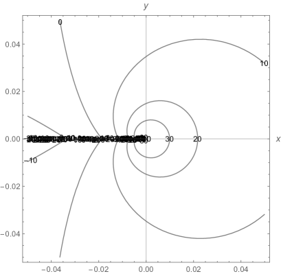
Figure 1: The stream lines of the normal current near the moving vortex for $s=0.05$. Positive contour numbers correspond to the clockwise direction of $\bm{j}_{n}$ whereas negative to the counterclockwise; $x,y$ are in units of $\lambda$. The cut at $x<0$ of the $x$ axis is traced to Eq. (16) for $E_{y}$ where at $y=0$ and negative $x$ the integral is not defined. $x,y$ are in units of $\lambda$.

Since the field $\bm{h}$ is directed out of the figure plane, the normal currents cause its reduction in front of the moving vortex and enhancement behind.

The total magnetic flux carried by a vortex is still $\phi_{0}$, so that appearance of normal currents should change the distribution of supercurrents as well:

$$\bm{j}_{s}=\bm{j}-\bm{j}_{n}=\frac{c\phi_{0}}{8\pi^{2}\lambda^{3}}\left(\hat{\bm{j}}-\frac{s}{2\pi}\hat{\bm{E}}\right)$$ (19)

where the under-hat quantities are dimensionless RHS’s in expressions (11), (12) for $\bm{J}$ and integrals in Eqs. (15), (16) for $\bm{E}$.

Of a particular interest is the distribution of the values $|\bm{j}_{s}|=\sqrt{j_{sx}^{2}+j_{sy}^{2}}$, because $|\bm{j}_{s}|$ cannot exceed the depairing value, thus defining qualitatively the “core boundary”.

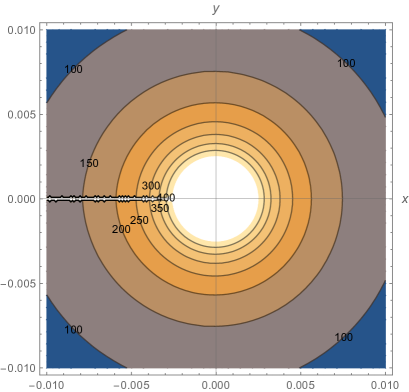
Figure 2: (Color online) Contours of constant values of the supercurrent $|j_{s}|$ near the moving vortex for $s=0.05$; $x,y$ are in units of $\lambda$.

Fig. 2 shows contours of constant $|j_{s}|$ for $s=0.05$ in the vicinity of the core. Hence, the moving vortex core in this case should be close to a circle; the anisotropy of $j_{s}$ is still seen, e.g., in the contour marked by 100, which is only slightly differs from a circle. In other words, despite the presence of normal currents lacking any resemblance of cylindrical symmetry, Fig. 1, the core shape of Abrikosov vortex is hardly affected by the vortex motion. We have checked that for a faster motion with $s=2$, to find $j_{s}(x,y)=\,\,$const near the singularity is close to a circle. This implies that for a moving Abrikosov vortex in the bulk the normal currents near the core are small and their effects on persistent currents are weak. As is shown below, the situation in thin films is drastically different.

III Thin films

We start this section with a few known general results and then apply them to moving Pearl vortices. Let the film of thickness $d$ be in the $xy$ plane. Integration of Eq. (3) over the film thickness gives for the $z$ component of the field at the film for a Pearl vortex moving with velocity $\bm{v}$:

$$\frac{2\pi\Lambda}{c}{\rm curl}_{z}{\bm{g}}+h_{z}+\tau\frac{\partial h_{z}}{\partial t}=\phi_{0}\delta(\bm{r}-\bm{v}t).$$ (20)

Here, $\bm{g}$ is the sheet current density related to the tangential field components at the upper film face by $2\pi\bm{g}/c=\hat{\bm{z}}\times\bm{h}$; $\Lambda=2\lambda^{2}/d$ is the Pearl length, and $\tau=4\pi\sigma\lambda^{2}/c^{2}$. With the help of div$\bm{h}=0$ this equation is transformed to:

$$h_{z}-\Lambda\frac{\partial h_{z}}{\partial z}+\tau\frac{\partial h_{z}}{\partial t}=\phi_{0}\delta(\bm{r}-\bm{v}t).$$ (21)

A large contribution to the energy of a vortex in a thin film comes from stray fields [10]. The problem of a vortex in a thin film is, in fact, reduced to that of the field distribution in free space subject to the boundary condition supplied by solutions of Eq. (20) at the film surface. Since outside the film curl$\bm{h}=\,\,\,$div$\bm{h}=0$ (see remark [11]), one can introduce a scalar potential for the outside field in the upper half-space:

$$\bm{h}=\bm{\nabla}\varphi,\qquad\nabla^{2}\varphi=0\,.$$ (22)

The general form of the potential satisfying Laplace equation that vanishes at $z\to\infty$ is

$$\varphi(\bm{r},z)=\int\frac{d^{2}\bm{k}}{4\pi^{2}}\varphi(\bm{k})e^{i\bm{k}\cdot\bm{r}-kz}\,.$$ (23)

Here, $\bm{k}=(k_{x},k_{y})$, $\bm{r}=(x,y)$, and $\varphi(\bm{k})$ is the two-dimensional Fourier transform of $\varphi(\bm{r},z=0)$. In the lower half-space one has to replace $z\to-z$ in Eq. (23).

As is done in [2], one applies the 2D Fourier transform to Eq. (21) to obtain a linear differential equation for $h_{z\bm{k}}(t)$. The solution is

$$h_{z\bm{k}}=-k\varphi_{\bm{k}}=\frac{\phi_{0}e^{-i\bm{k}\cdot\bm{v}t}}{1+\Lambda k-i\bm{k}\cdot\bm{v}\tau}\,$$ (24)

and

$$\varphi_{\bm{k}}=-\frac{\phi_{0}e^{-i\bm{k}\cdot\bm{v}t}}{k(1+\Lambda k-i\bm{k}\cdot\bm{v}\tau)}\,.$$ (25)

In fact, this gives distributions of all field components outside the film, its surface included.

We are interested in the vortex motion with constant velocity $\bm{v}=v\hat{\bm{x}}$, so that we can evaluate this field in real space for the vortex at the origin at $t=0$:

$$h_{z}(\bm{r})=\frac{\phi_{0}}{4\pi^{2}}\int\frac{d^{2}\bm{k}\,e^{i\bm{k}\cdot\bm{r}}}{1+\Lambda k-ik_{x}v\tau}\,.$$ (26)

It is convenient in the following to use Pearl $\Lambda$ as the unit length and measure the field in units $\phi_{0}/4\pi^{2}\Lambda^{2}$:

$$h_{z}(\bm{r})=\int\frac{d^{2}\bm{k}\,e^{i\bm{k}\cdot\bm{r}}}{1+k-ik_{x}s}\,,$$ (27)

we left the same notations for $\bm{h}_{z}$ and $\bm{k}$ in new units; when needed, we indicate formulas written in common units. The parameter

$$s=\frac{v\tau}{\Lambda}=2\pi\frac{v\sigma d}{c^{2}}\,,$$ (28)

so that $s\ll 1$ for most practical situations. However, in recent experiments the velocities $1.5\times 10^{6}\,$cm/s were recorded, for which $s$ might reach $0.1$ which may still increase in future experiments [12, 13]. Besides, vortices exist not only in low temperature laboratories, but e.g. in neutron stars about their motion we know little. Hence, in the derivations below we consider arbitrary values of $s$.

After applying the same formal procedure as for 3D Abrikosov vortex one obtains [4]:

$$h_{z}(\bm{r})=2\pi\int_{0}^{\infty}du\frac{u\,e^{-u}}{(\rho^{2}+u^{2})^{3/2}}$$ (29)

with $\rho^{2}=(x+us)^{2}+y^{2}$. Hence, we succeeded in reducing the double integral (27) to a single integral over $u$ which is readily evaluated.

The results are shown in Fig. 3. The field distribution is not symmetric relative to the singularity position: the field in front of the moving vortex is suppressed relative to the symmetric distribution of the vortex at rest, whereas behind the vortex it is enhanced [4].

Integrating by parts we obtain from Eq. (29):

$$h_{z}=2\pi\left[\frac{1}{r}-\int_{0}^{\infty}\frac{du\,e^{-u}}{\sqrt{\rho^{2}+u^{2}}}\left(1+\frac{s(x+su)}{\rho^{2}+u^{2}}\right)\right].\qquad$$ (30)

For the Pearl vortex at rest $s=0$, $\rho=r$, and the known result for a vortex at rest follows, see e.g. Ref. [14]. In particular, the last form of $h_{z}(x,y)$ shows that as $r\to 0$ the leading term of this field diverges as $1/r$, i.e., faster than $|\ln r|$ of the Abrikosov vortex in the bulk [14, 15].

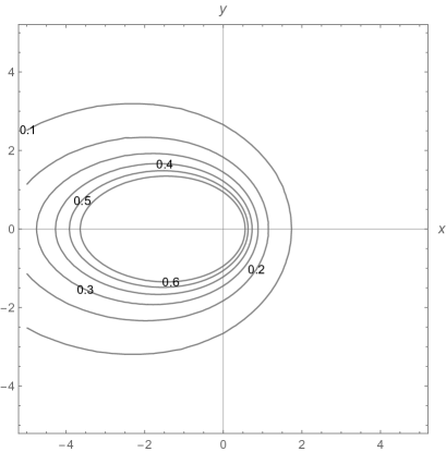
Figure 3: Contours of $h_{z}(x,y)=\,\,$const ($h_{z}$ is in units $\phi_{0}/4\pi^{2}\Lambda^{2}$ and $x,y$ in units of $\Lambda$) for $s=2$. $x,y$ are in units of $\Lambda$.

For the most realistic slow motion with $s\ll 1$, one can get analytic approximation for the field distribution. To this end, go back to Eq. (29) and expand the integrand in powers of small $s$ up to ${\cal O}(s)$:

$$h_{z}=2\pi\left(\int_{0}^{\infty}\frac{du\,u\,e^{-u}}{(r^{2}+u^{2})^{3/2}}+3sx\int_{0}^{\infty}\frac{du\,u^{2}e^{-u}}{(r^{2}+u^{2})^{5/2}}\right).\qquad$$ (31)

The first term gives the field of the vortex at rest. The second term is:

$$-s\,x\left[\frac{2}{r}+\frac{\pi}{2}(Y_{0}-\bm{H}_{0})_{r}+\frac{\pi}{2r}(Y_{1}-\bm{H}_{1})_{r}\right]\,,$$ (32)

where $Y_{0,1}$ and $\bm{H}_{0,1}$ are Bessel and Struve functions of argument $r$.

IV Current distribution

As mentioned above, the sheet current is related to the tangential field components by

$$\frac{2\pi}{c}g_{x}=-h_{y}\,,\qquad\frac{2\pi}{c}g_{y}=h_{x}\,.$$ (33)

In 2D Fourier space, tangential fields are $h_{x\bm{k}}=ik_{x}\varphi_{\bm{k}}$ and $h_{y\bm{k}}=ik_{y}\varphi_{\bm{k}}$. The potential at $t=0$ and $z=+0$ is given (in common units) by

$$\varphi_{\bm{k}}=-\frac{\phi_{0}}{k(1+\Lambda k-ik_{x}v\tau)}.$$ (34)

Then, we have:

$$g_{x}(\bm{r},s)=-i\frac{c\phi_{0}}{2\pi\Lambda^{2}}I_{x}\,,\quad I_{x}=\int\frac{d\bm{k}\,k_{y}e^{i\bm{k}\bm{r}}}{k(1+k-ik_{x}s)},\qquad$$ (35)

$$g_{y}(\bm{r},s)=i\frac{c\phi_{0}}{2\pi\Lambda^{2}}I_{y}\,,\quad I_{y}=\int\frac{d\bm{k}\,k_{x}e^{i\bm{k}\bm{r}}}{k(1+k-ik_{x}s)}.\qquad$$ (36)

To evaluate dimensionless integrals $I_{x,y}$ we make use of the identity (7) in which $k^{2}\to k$:

$$I_{x} = \int\frac{d\bm{k}\,k_{y}e^{i\bm{k}\bm{r}}}{k}\int_{0}^{\infty}du\,e^{-u(1+k-ik_{x}s)}$$ (37)

$$= \int_{0}^{\infty}du\,e^{-u}\int\frac{d\bm{k}\,k_{y}}{k}e^{i\bm{k}\bm{\rho}-uk}$$

To evaluate here the integral over $\bm{k}$, we make use of the Coulomb Green’s function which can be manipulated to the form [4]:

$$\frac{1}{\sqrt{x^{2}+y^{2}+z^{2}}}=\frac{1}{2\pi}\int\frac{d^{2}\bm{k}}{k}e^{i\bm{k}\bm{r}-kz}.\qquad$$ (38)

Replace now $\bm{r}\to\bm{\rho}=(x+us,y)$, $z\to u$:

$$\frac{1}{\sqrt{(x+us)^{2}+y^{2}+u^{2}}}=\frac{1}{2\pi}\int\frac{d\bm{k}}{k}e^{i\bm{k}\bm{\rho}-ku}\qquad$$ (39)

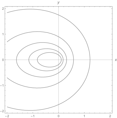
Figure 4: Contours of constant potential $\varphi(x,y)$ and, what is the same, the stream lines of the current $\bm{g}$ for a fast moving vortex, $s=2$. $x$ and $y$ are in units of $\Lambda$.

and apply $\partial_{y}$ to get the integral over $\bm{k}$ in Eq. (37):

$$-\frac{y}{(\rho^{2}+u^{2})^{3/2}}=\frac{i}{2\pi}\int\frac{d\bm{k}\,k_{y}}{k}e^{i\bm{k}\bm{\rho}-ku}.\qquad$$ (40)

Hence, we obtain

$$\frac{\Lambda^{2}}{c\phi_{0}}\,g_{x}=y\int_{0}^{\infty}\frac{du\,e^{-u}}{(\rho^{2}+u^{2})^{3/2}},\qquad$$ (41)

and

$$\frac{\Lambda^{2}}{c\phi_{0}}\,g_{y}=-\int_{0}^{\infty}\frac{du\,e^{-u}(x+us)}{(\rho^{2}+u^{2})^{3/2}}.\qquad$$ (42)

It is easy to see that stream lines of the total current coincide with contours of $\varphi(x,y)=\,\,$const. These are shown in Fig. 4, so that for a fast motion the current distribution differs substantially from the static case.

It is worth noting that the currents in Eqs. (41) and (42) are in fact total, i.e. the sum of persistent and normal currents, $\bm{g}=\bm{g}_{s}+\bm{g}_{n}$. It is of interest to separate these contributions, because the size and shape of vortex cores are related to the value of persistent currents only. As was done for the Abrikosov vortex, we calculate first the normal currents $\bm{g}_{n}=\sigma\bm{E}d$.

IV.1 Normal currents

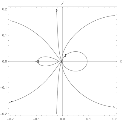
Figure 5: Stream lines of the normal current, i.e., the lines of $S(x,y)=\,\,$const, for a slow motion with $s=0.05$. $x$ and $y$ are units of $\Lambda$. The positive values of $S$ correspond to clockwise direction of $\bm{g}_{n}$ and negative for counterclockwise.

To this end, one takes the magnetic field of moving vortex, Eq. (24), and obtains the electric field from Maxwell equations $i({\bm{k}}\times{\bm{E}}_{\bm{k}})_{z}=-\partial_{t}h_{z{\bm{k}}}/c$ and ${\bm{k}}\cdot{\bm{E}}_{\bm{k}}=0$:

$$E_{x{\bm{k}}} = -\frac{\phi_{0}v}{c}\frac{k_{x}k_{y}}{k^{2}(1+k-ik_{x}s)}\,,$$ (43)

$$E_{y{\bm{k}}} = \frac{\phi_{0}v}{c}\frac{k_{x}^{2}}{k^{2}(1+k-ik_{x}s)}$$ (44)

($\Lambda$ is used as the unit length).

The stream lines of the normal current $\bm{g}_{n}$ coincide with those for $\bm{E}$ which satisfy $0=(d\bm{\ell}\times\bm{E})_{z}=dxE_{y}-dyE_{x}$. Introducing $S(x,y)$ such that

$$E_{y}=\frac{\partial S}{\partial x},\qquad E_{x}=-\frac{\partial S}{\partial y}\,,$$ (45)

we see that the stream lines of the vector field $\bm{E}$ are given by $S(x,y)=\,\,$const. Using Eqs. (43) or (44) we obtain in Fourier space

$$S_{\bm{k}}=\frac{k_{x}}{ik^{2}(1+k-ik_{x}s)}$$ (46)

and

$$S(\bm{r})=\int\frac{d\bm{k}\,k_{x}e^{i\bm{k}\bm{r}-kz}}{k^{2}(1+k-ik_{x}s)}$$ (47)

where constant pre-factors are omitted. Making use of identity (39) we arrive at

$$S(\bm{r}) = \int_{0}^{\infty}du\,e^{-u}\frac{x+us}{{\cal R}({\cal R}+u)}\,,$$ (48)

$${\cal R}^{2} = (x+us)^{2}+y^{2}+u^{2}=\rho^{2}+u^{2}\,.$$ (49)

The electric field is now obtained with the help of Eq. (45):

$$\frac{2\pi\Lambda^{2}c}{\phi_{0}v}E_{x}(\bm{r})=-\int_{0}^{\infty}du\,e^{-u}\frac{y(x+us)(u+2{\cal R})}{{\cal R}^{3}(u+{\cal R})^{2}}\,,\qquad$$ (50)

$$\frac{2\pi\Lambda^{2}c}{\phi_{0}v}E_{y}(\bm{r})$$

$$=\int_{0}^{\infty}du\,e^{-u}\frac{{\cal R}^{2}(u+{\cal R})-(x+us)^{2}(u+2{\cal R})}{{\cal R}^{3}(u+{\cal R})^{2}}.\qquad$$ (51)

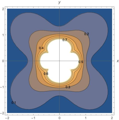
Figure 6: (Color online) Contours of constant normal current values $\sqrt{g_{nx}^{2}+g_{ny}^{2}}$ for a moving vortex with $s=0.05$. $x$ and $y$ are in units of $\Lambda$, so that one can say this figure represents the distribution at large distances.

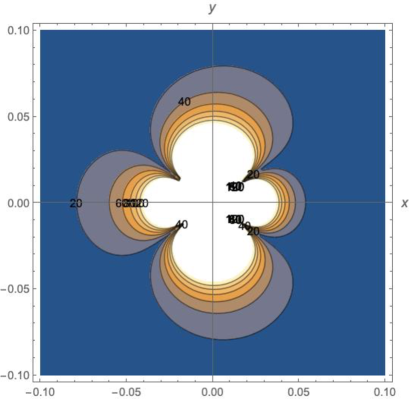
Figure 7: (Color online) Contours of constant normal current values $\sqrt{g_{nx}^{2}+g_{ny}^{2}}$ for a moving vortex with $s=0.05$ at short distances. $x$ and $y$ are in units of $\Lambda$.

Fig. 5 show the stream lines of normal currents (in fact these are contours of constant $S(x,y)$) for a fast and slow motion.

Figs. 6 and 7 show the distribution of normal current values at large and short distances for $s=0.05$. The exotic shape of these distributions close to the core signals to possible peculiarities of supercurrents as well.

To make sense of the “cloverleaf” shape of the normal current distributions, let us look at the $\bm{E}$ components of Eqs. (50), (51) for slow motion $s\ll 1$. Note that the pre-factor $\phi_{0}v/2\pi\lambda^{2}c\propto v\propto s$, so that for $s\to 0$ one can set $s=0$ in the integrals over $u$:

$$E_{x}\propto-s\int_{0}^{\infty}du\,e^{-u}\frac{yx(u+2{\cal R}_{1})}{{\cal R}_{1}^{3}(u+{\cal R}_{1})^{2}},$$ (52)

$$E_{y}=s\int_{0}^{\infty}du\,e^{-u}\frac{{\cal R}_{1}^{2}(u+{\cal R}_{1})-x^{2}(u+2{\cal R}_{1})}{{\cal R}_{1}^{3}(u+{\cal R}_{1})^{2}}.\qquad$$ (53)

where ${\cal R}_{1}^{2}=r^{2}+u^{2}$. We note that in polar coordinates $x=r\cos\varphi,\,\,\,y=r\sin\varphi$, ${\cal R}_{1}$ depends only on $r$. Hence, we can write these equations as

$$E_{x}=A(r)\sin 2\varphi,\quad E_{y}=B(r)-C(r)\cos^{2}\varphi\,\qquad$$ (54)

where $A(r),B(r),C(r)$ should be evaluated by integrations over $u$. But even without integrations it is clear that the value $|\bm{E}|=\sqrt{E_{x}^{2}+E_{y}^{2}}$ depends on the azimuth $\varphi$. The same is true for $|\bm{g}_{n}|$. A simple example of the azimuthal dependence is shown in Fig. 8 for some set of $A,B,C$.

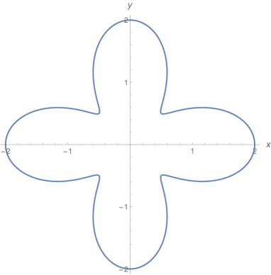
Figure 8: Contours of constant values $\sqrt{E_{x}^{2}+E_{y}^{2}}$ according to Eq. (54) with $A=0.7$, $B=2$, and $C=4$.

Thus, the unusual distributions of $|\bm{g}_{n}|$ at short distances from the vortex center can be traced to azimuth dependent divergences of $\bm{g}_{n}$ when one approaches the vortex core.

IV.2 Persistent currents

The normal sheet current density is $\bm{g}_{n}=\sigma\bm{E}\,d$, whereas the supercurrent is $\bm{g}_{s}=\bm{g}-\bm{g}_{n}$, so that

$$g_{sx}=g_{x}-g_{nx}=\frac{c\phi_{0}}{\Lambda^{2}}(\hat{g}_{x}-\frac{s}{4\pi^{2}}\hat{E}_{x})\,,$$ (55)

where $\hat{g}_{x}$ and $\hat{E}_{x}$ are the dimensionless integrals of Eqs. (41) and (50). In particular, this reflects the fact that normal currents disappear at $v=0$. Similarly, we have

$$g_{sy}=g_{y}-g_{ny}=\frac{c\phi_{0}}{\Lambda^{2}}(\hat{g}_{y}-\frac{s}{4\pi^{2}}\hat{E}_{y})\,.$$ (56)

As mentioned, the vortex core cannot be described by the London theory, but the distribution of $\bm{g}_{s}(\bm{r})$ outside the core may affect its shape [16]. A qualitative picture of the core shape can be obtained by examining contours of the current values $|\bm{g}_{s}(x,y)|=\,\,\,$const outside the core. This is shown in Fig. 9 and 10.

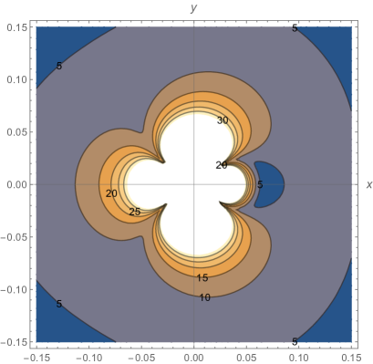
Figure 9: (Color online) Contours of constant supercurrent values $\sqrt{g_{sx}^{2}+g_{sy}^{2}}$ for a moving vortex with $s=0.05$. $x$ and $y$ are in units of $\Lambda$. One can see that the anisotropy of this distribution decreases with the distance from the vortex singularity.

One can see that the distortion of supercurrents near the vortex core disappears with increasing distance from the core.

The London current $g_{s}$ diverges if $r\to 0$. One can define qualitatively the core “boundary” as a curve where the London current reaches the depairing value, $j_{d}=c\phi_{0}/16\pi^{2}\lambda^{2}\xi$ for the bulk or $g_{d}=c\phi_{0}/8\pi^{2}\Lambda\xi$ for thin films, see e.g. Ref. [16]. For the Abrikosov vortex at rest in isotropic bulk case this simple procedure gives the coherence length $\xi$ as the core size. An example of the core shape so defined for a moving vortex is given in Fig. 10.

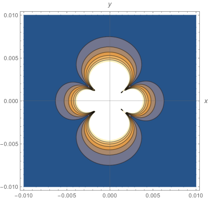
Figure 10: (Color online) Contours of constant supercurrent values $\sqrt{g_{sx}^{2}+g_{sy}^{2}}$ for a moving vortex with $s=0.05$ at short distances. $x$ and $y$ are in units of $\Lambda$.

The persistent currents of the Pearl vortex at rest diverge as $const/r$ when $r\to 0$, see e.g. [14]. But for a moving vortex, the constant here may depend on the direction along which the origin is approached. As we have seen, the total magnetic flux carried by vortex is $\phi_{0}$, therefore, appearance of normal currents in moving vortex will cause redistribution of supercurrents as well, in particular, near the singularity this redistribution is substantial because normal currents diverge there, too, see Figs. 6 and 7. This may result in exotic shapes of the lines of constant $|g_{s}(x,y)|$ at short distances from the singularity.

V Discussion

We have shown that the magnetic structure of the moving vortices is distorted relative to the vortex at rest. The flux quantum of a moving vortex is redistributed, the back side part of the flux is enhanced, whereas the in-front part is depleted. Physically, the distortion is caused by normal currents arising due to changing in time magnetic field at each point of space, the electric field is induced and causes normal currents.

Distributions of both normal and persistent currents have been considered for moving Abrikosov vortices in the bulk and for Pearl vortices in thin films. It turned out for films that these distributions at distances $r$ small on the scale of the Pearl $\Lambda$ have exotic shapes shown in Figs. 8, 9.

This finding is potentially relevant because the vortex core shape might be affected by persistent currents out of the core, if the core “boundary” is defined as the place where the outside supercurrents reach the depairing value, the concept introduced by L. D. Landau in his theory of superfluidity [18]. Our calculations show that if one approaches the vortex singularity along a straight line at an angle $\varphi$ with velocity (directed along $x$), the depairing value is reached at the azimuth dependent $r(\phi)$. Validity of such a definition of the core boundary should be confirmed, of course, by microscopic calculations of the order parameter $\Delta(r,\varphi)$ inside the core, the problem out of the scope of this work. Our intention is to address this question in near future.

If our picture is confirmed, the problem will arise about the structure of the inside-the-core quasi-particle states in moving vortices which can differ substantially from the states in the vortex at rest [17].

Uncommon core current distributions of moving vortices in isotropic materials is due to the vector of velocity that breaks the cylindrical symmetry of fields and currents. In other words, the problem becomes anisotropic. This leads to an idea that in anisotropic superconductors similar distributions might occur even in vortices at rest. We plan to present our results for this case in a separate publication.

There are experimental techniques which, in principle, could probe the field distribution in moving vortices [12]. This is a highly sensitive SQUID-on-tip with the loop small on the scale of possible Pearl lengths. Recent experiments have traced vortices moving in thin films with velocities well above the speed of sound [12, 13]. Vortices crossing thin-film bridges being pushed by transport currents have a tendency to form chains directed along the velocity. The spacing of vortices in a chain is usually exceeds by much the core size, so that commonly accepted reason for the chain formation, namely, the depletion of the order parameter behind moving vortices is questionable. But at distances $r\gg\xi$ the time dependent London theory is applicable. Another promising technique of studying moving vortices could be Tonomura’s Lorentz Microscopy [19].

VI Acknowledgements

The work of V.K. was supported by the U.S. Department of Energy (DOE), Office of Science, Basic Energy Sciences, Materials Science and Engineering Division. Ames Laboratory is operated for the U.S. DOE by Iowa State University under contract # DE-AC02-07CH11358.

References

- [1] L. Radzihovsky, Phys. Rev. Lett. 115, 247801 (2015). DOI: 10.1103/PhysRevLett.115.247801
- [2] V. G. Kogan, Phys. Rev. B97, 094510 (2018).
- [3] V. G. Kogan and R. Prozorov, Phys. Rev. B102, 024506 (2020). DOI: 10.1103/PhysRevB.102.024506
- [4] V. G. Kogan and N. Nakagawa, Condens. Matter, 4, 6 (2021). https://doi.org/10.3390/condmat6010004.
- [5] P. de Gennes, Superconductivity of Metals and Alloys (Benjamin, New York, 1966).
- [6] G. Blatter, M. V. Feigelman, V. B. Geshkenbein, A. I. Larkin, V. M. Vinokur, Rev. Mod. Phys., 66, 1125 (1994).
- [7] M. Smith, A. V. Andreev, and B. Z. Spivak, Phys. Rev. B101, 134508 (2020). DOI:https://doi.org/10.1103/PhysRevB.101.134508
- [8] L. P. Gor’kov and N. B. Kopnin, Usp. Fiz. Nauk, 116, 413 (1975); Sov. Phys.-Usp., 18, 496 (1976).
- [9] Throughout this paper we use numerical integrations for integrals over similar to that in the first line of Eq. (10) to obtain fields or current distributions singular at the origin. Since this equation also provides the exact result in the second line, we compared analytic outcomes with numerical ones obtained with the help of Mathematica and found relative differences on the order of .
- [10] J. Pearl, Appl. Phys. Lett 5, 65 (1964).
- [11] The electric field in vacuum can be neglected since out of the film and . In other words, the electro-magnetic radiation is disregarded.
- [12] L. Embon, Y. Anahory, Ž.L. Jelić, E.O.Lachman, Y. Myasoedov, M. E. Huber, G. P. Mikitik, A. V. Silhanek, M. V. Milosević, A. Gurevich, and E. Zeldov, Nat. Commun. 8, 85 (2017).
- [13] O. V. Dobrovolskiy, D. Yu. Vodolazov, F. Porrati, R. Sachser, V. M. Bevz, M. Yu. Mikhailov, A. V. Chumak, and M. Huth, Nature Communications 11, 3291 (2020); arXiv:2002.08403.
- [14] V. G. Kogan, V. V. Dobrovitski, J. R. Clem, Y. Mawatari, and R. G. Mints, Phys. Rev. BB, 63, 144501 (2001). DOI: 10.1103/PhysRevB.63.144501
- [15] F. Tafuri, J.R. Kirtley, P.G. Medaglia, P. Orgiani, and G. Balestrino, Phys. Rev. Lett. 92, 157006 (2004).
- [16] V. G. Kogan and M. Ichioka, J. Phys. Soc. Jpn, 89, 094711 (2020). https://doi.org/10.7566/JPSJ.89.094711
- [17] C. Caroli, P. G. deGennes, and J. Matricon, Phys. Let. 9, 307 (1964).
- [18] E. M. Lifshitz and L. P. Pitaevsky, Statistical Physics, part 2, Pergamon, Oxford - New York, 1959.
- [19] J. E. Bonevich, K. Harada, T. Matsuda, H. Kasai, T. Yoshida, G. Pozzi, and A. Tonomura, Phys. Rev. Lett. 70, 2952 (1993).