Non-invasive multigrid for semi-structured grids

Abstract

Multigrid solvers for hierarchical hybrid grids (HHG) have been proposed to promote the efficient utilization of high performance computer architectures. These HHG meshes are constructed by uniformly refining a relatively coarse fully unstructured mesh. While HHG meshes provide some flexibility for unstructured applications, most multigrid calculations can be accomplished using efficient structured grid ideas and kernels. This paper focuses on generalizing the HHG idea so that it is applicable to a broader community of computational scientists, and so that it is easier for existing applications to leverage structured multigrid components. Specifically, we adapt the structured multigrid methodology to significantly more complex semi-structured meshes. Further, we illustrate how mature applications might adopt a semi-structured solver in a relatively non-invasive fashion. To do this, we propose a formal mathematical framework for describing the semi-structured solver. This formalism allows us to precisely define the associated multigrid method and to show its relationship to a more traditional multigrid solver. Additionally, the mathematical framework clarifies the associated software design and implementation. Numerical experiments highlight the relationship of the new solver with classical multigrid. We also demonstrate the generality and potential performance gains associated with this type of semi-structured multigrid.

1 Introduction

Multigrid (MG) methods have been developed for both structured and unstructured grids [7, 15, 20, 23]. In general, unstructured meshes are heavily favored within sophisticated science and engineering simulations as they facilitate the representation of complex geometric features. While unstructured approaches are often convenient, there are significant potential advantages to structured meshes on exascale systems in terms of memory, setup time, and kernel optimization. In recent years, multigrid solvers for hierarchical hybrid grids (HHGs) have been proposed to provide some flexibility for unstructured applications while also leveraging some features of structured multigrid for performance on advanced computing systems [3]. Hierarchical hybrid grids are formed by regular refinement of an initial coarse grid. The result is a HHG grid hierarchy containing regions of structured mesh, even if the initial coarse mesh is completely unstructured [3]. Essentially, each structured region in an HHG mesh corresponds to one element of the original coarse mesh that has been uniformly refined. A corresponding multigrid solver can then be developed using primarily structured multigrid ideas. Figure 1 illustrates a two dimensional HHG mesh hierarchy with three structured regions. Here, the two rightmost grids might be used as multigrid coarse grids for a discretization on the finest mesh.

Fig. 1: A hierarchy of two dimensional HHG meshes created by regular refinement of a 3 element mesh

The key point is that structured multigrid kernels can be used for most of the computation. These structured computations require significantly less memory and generally less communication than their unstructured counterparts. Further, the structured multigrid kernels are significantly more amenable to performance optimization on advanced architectures. A series of papers [2, 4, 13, 11, 12, 14] have documented noticeably impressive HPC performance using an HHG approach on realistic simulations, some involving over one trillion unknowns. In these papers, the primarily structured nature of the mesh is heavily leveraged throughout the multigrid solver in an essentially matrix-free fashion.

While HHG solvers provide some balance between flexibility and structured performance, they do impose restrictions on the type of meshes that can be considered. Additionally, it is difficult to adapt existing finite element applications to HHG solvers. Of course there are alternative approaches to structure including composite grids, overset meshes, and octree meshes (for example [18, 9, 16, 21, 17, 22]). Additionally, Hypre has some semi-structured capabilities [10]. While these approaches can also attain good scalability on high performance architectures, most scientific teams have been resistant to investigate these structured grid possibilities due to concerns about their intrusive nature, often requiring fundamental changes to the mesh representations and discretization technology employed within the application. This is especially true for unstructured finite element simulations, which dominate the discretization approaches employed at Sandia.

Our aim in this paper is to at least partially address these obstacles by broadening the HHG approach to a wider class of meshes and by providing an easier or less-invasive code path to migrate existing applications toward semi-structured solvers. To do this, we introduce a mathematical framework centered around the idea of a region representation. The region perspective decomposes the original domain into a set of regions that only overlap at inter-region interfaces and where the computational mesh also conforms at these interfaces. The main difference from the typical situation (which we refer to as the composite mesh to emphasize the differences) is that each region has its own copy of solution unknowns along its interfaces. If all regions are structured, the overall grid is a block structured mesh (BSM). BSMs can be constructed by joining separately meshed components or a regular refinement of an unstructured mesh as in the HHG case. Thus, BSMs are a generalization of the HHG idea. As in the HHG case, a special region-oriented solver can take advantage of structure within structured regions.

The mathematical framework allows us to consider region-oriented versions of algorithms developed from a traditional composite mesh perspective. It also provides conditions on the region-oriented grid transfer operators to guarantee a mathematical equivalence relationship between region-oriented multigrid and a traditional solver. In some cases, it is easy to accomplish this exact equivalence while in other cases there are practical tradeoffs that must be weighed, comparing additional computational/communication requirements against a possible convergence benefit to exact equivalence. One key result of the mathematical framework is that in some cases (linear interpolation grid transfers without curved region interfaces) it is possible to construct a region multigrid hierarchy without communication. This includes no communication requirement for the Galerkin triple matrix product (used to project the discretization operator) when all associated matrices adopt a region representation. This is in contrast to a standard AMG setup algorithm where communication costs can be noticeable especially when the density of the discretization sparsity pattern increases as one constructs coarser and coarser matrices.

The mathematical framework is fairly general in that it is not restricted to structured regions. That is, it allows for the possibility that some regions might be structured while others are unstructured. This can be useful in applications where it might be awkward to resolve certain geometries or to capture local features with only structured regions. Figure 2 illustrates some partially structured meshes. The leftmost image corresponds to a mesh used to represent wires. The middle picture illustrates a main body mesh with an attached part. The rightmost example displays a background mesh with some split elements to represent an interface. In this last case, an unstructured region might be employed only to surround the interface.

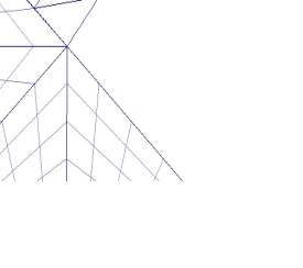
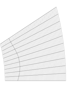
Fig. 2: Radial tri-section mesh (left), unstructured region attached to an HHG mesh (middle), interface with cut element mesh (right).

Our software considers these types of situation again using the mathematical framework as a guide for the treatment of grid transfer operators near region interfaces. Of course, a matrix-free approach would be problematic in this more general setting and performance in unstructured regions might be poorer, though there will be much fewer unstructured regions.

One nice aspect of the mathematical framework is that it formalizes the transformation between composite and region perspectives. As noted, this is helpful when designing grid transfers near region interfaces. It is also helpful, however, when understanding the minimal application requirements for employing such a region-oriented solver. In particular, the finite element software must provide a structured PDE matrix for each structured region as well as more detailed information on how to glue regions together. It is easy for the requirements of a semi-structured or an HHG framework to become intrusive on the application infrastructure. The philosophy taken in this paper is toward the development of algorithms and abstractions that are sufficiently flexible to model complex features without imposing over-burdensome requirements. To this end, we propose a software framework that transforms a standard fully assembled discretization matrix (that might be produced with any standard finite element software) into a series of structured matrices. Of course, the underlying mesh used with the finite element software must coincide with a series of structured regions (e.g., as in Figure 1). Additionally, the finite element software must provide some minimal information about the underlying structured region layout.

An overall semi-structured solver is being developed within the Trilinos framework in conjunction with the Trilinos/MueLu [5, 6] multigrid package. This solver is not oriented toward matrix-free representations in favor of greater generality, though some matrix-free performance/memory benefits are sacrificed. The ideas described in this paper are intended to facilitate the use of semi-structured solvers within the finite element community and to ultimately provide significant performance gains over existing fully unstructured algebraic multigrid solvers (such as those provided by MueLu). Section 2 motivates and describes some semi-structured mesh scenarios. Section 3 is the heart of the mathematical framework, describing the key kernels and their equivalence to a standard composite grid multigrid scheme. Here, the V-cycle application relies heavily on developing a matrix-vector product suitable for matrices stored in a region-oriented fashion. We also detail the hierarchy setup, focusing on the construction of region-oriented matrices to represent grid transfers and the coarse discretization matrix. Section 4 describes the framework and the non-invasive application requirements while Section 5 discusses unstructured regions focusing on the treatment of multigrid transfer operators at region interfaces. We conclude with some numerical experiments to highlight the potential of such a semi-structured multigrid solver.

2 Semi-structured grids and mesh abstractions

Unstructured meshes facilitate the modeling of complex features, but induce performance challenges. Our goal is to provide additional mechanisms to address unstructured calculations while furnishing enough structure to reap performance benefits. Our framework centers around block structured meshes (BSMs). In our context, it is motivated by an existing Sandia hypersonic flow capability where the solution quality obtained with block structured meshes is noticeably superior than solutions obtained with fully unstructured meshes.

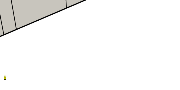
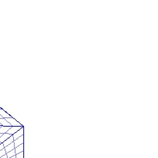
Fig. 3: Hypersonic BSM domain (outline of region boundaries depicted; structured grid lines not shown) and BSM/HHG mesh.

In this case, BSMs generated by meshing separate components are of significantly greater interest than meshes of the HHG variety. Figure 3 illustrates a general BSM and a BSM/HHG mesh.

While BSMs provide a certain degree of flexibility, unstructured meshes are often natural to capture complex features locally. Figure 2 illustrates some scenarios where unstructured regions might be desirable. Figure 4 shows another case which is similar to our motivating/target hypersonic example. In our hypersonic problem, refined structured meshes are needed in sub-domains upstream of the obstacle. In the wake area, however, much lower resolution meshes (and unstructured meshes) can be employed. In this case, unstructured mesh regions can be used to

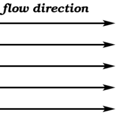
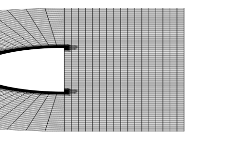
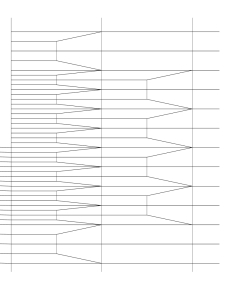
Fig. 4: Primarily structured mesh with small unstructured regions (left) with a close up view of one of the unstructured regions (right).

transition between structured meshes where modeling characteristics allow for a large difference in resolutions. Specifically, two conformal structured meshes could have been used to represent the domain in Figure 4 (one upstream and the other in the wake). However, the use of small unstructured mesh regions allows for a much coarser version of the wake mesh, even though most of the wake can still be represented with structured mesh regions.

Our ultimate target is a mesh that includes an arbitrary number of structured or unstructured regions that conform at region interfaces. In this ideal setting, a finite element practitioner would have complete freedom to decide the layout of the mesh regions that is most suitable for the application of interest. Of course, such a mesh must be suitably partitioned over processors so that the structured regions can take advantage of structured algorithms and that the overall calculation is load balanced. Here, load balance must take into account that calculations in unstructured regions will likely be less efficient than those in structured regions. While our framework has been designed with this ultimate target in mind, some aspects of the present implementation limit the current software to the restriction of one region per processor.

3 Region-oriented multigrid

We sketch the main ideas behind a region-oriented version of a multigrid solver. In some cases, this region-oriented multigrid is mathematically identical to a classical multigrid solver, though implementation of the underlying kernels will be different. In other cases, it is natural to introduce modest numerical changes to the region-oriented version (e.g., a region-local Gauss–Seidel smoother). To simplify notation, we describe only a two level multigrid algorithm, as the extension to the multilevel case is straight-forward. Figure 5 provides a high-level illustration of the setup and solve phases of a classical two level multigrid algorithm.

$\text{function}\;\textsf{mgSetup}{(}A,\Psi)$		$\text{function}\;\textsf{mgCycle}({A},\,{u},\,{b}):$
	$\textsf{sData}\leftarrow\textsf{smootherSetup}{(}A)$		$\,{u}\leftarrow\mathcal{S}({A},\,{u},\,{b},\textsf{sData})$
	$P~{}~{}~{}~{}~{}\leftarrow\textsf{construct}P({A})$		$\,{r}\leftarrow\,{b}-{A}\,{u}$
	$R~{}~{}~{}~{}~{}\leftarrow P^{T}$		$\,{\mathrm{bar}{u}}\leftarrow 0$
	${\mathrm{bar}{A}}~{}~{}~{}~{}~{}\leftarrow RAP$		$\,{\mathrm{bar}{u}}\leftarrow\textsf{solve}({\mathrm{bar}{A}},\,{\mathrm{bar}{u}},{R}\,{r})$
			$\,{u}\leftarrow\,{u}+{P}\,{\mathrm{bar}{u}}$

Fig. 5: Two level multigrid for the solution of ${A}\,{u}=\,{b}$.

Therein, $A$ refers to the discretization operator on the fine level of the multigrid hierarchy. ${\cal S}$ denotes the fine level multigrid smoother. $P$ interpolates solutions from the coarse level to the fine level while $R$ restricts residuals from the fine level to the coarse level. sData refers to any pre-computed quantities that might be used in the smoother (e.g., ILU factors). Coarse level matrices and vectors are delineated by over bars (e.g., $\mathrm{bar}{A}$ is the coarse level discretization matrix and $\mathrm{bar}{u}$ is the coarse level correction). In this paper, $R$ is always taken as the transpose of $P$, though the ideas easily generalize to other choices for $R$. Finally, the coarse discretization is defined by the projection

$$\mathrm{bar}{A}=RAP.$$

For a two-level method, $\textsf{solve}()$ might correspond to a direct factorization solution method or possibly coarse level smoother sweeps. In these cases, $\textsf{mgSetup}()$ must include the setup of the $LU$ factors or coarse level smoothing data. A multilevel algorithm is realized by instead defining $\textsf{solve}()$ to be a recursive invocation of $\textsf{mgCycle}()$.

The region-oriented multigrid cycle is identical to this standard cycle. The only differences are that

• $A,\mathrm{bar}{A},R,$ and $P$ are stored in a region-oriented format,

• all vectors (e.g., approximate solutions, residuals) are stored in a region-oriented format,

• all operations (e.g., smoothing kernels) are implemented in a region-oriented fashion with the exception of the coarsest direct solve.

To describe region-oriented multigrid, we begin with a definition of the region layout for vectors and matrices. The creation of region-oriented matrices and vectors is delineated in two parts. The first part focuses on the hierarchy construction of region-oriented operators when region-oriented operators are provided on the finest level. The second part then proposes a mechanism for generating the finest level region-oriented operators using information that a standard finite element application can often supply.

3.1 Region matrices and vectors

Consider the discretization of a partial differential equation (PDE) and boundary conditions on a domain $\Omega$ resulting in the discrete matrix problem

$${A}u=b.$$

Often we will refer to the $n\times n$ matrix ${A}$ as the composite matrix. Consider now a decomposition of the domain $\Omega$ into a set of $m$ sub-regions ${\Omega}^{(i)}$ such that

$$\Omega=\cup_{i=1}^{m}~{}{\Omega}^{(i)}.$$

These regions only overlap at interfaces where they meet (e.g., see Figure 6). That is,

$$\mathrm{\Gamma}_{ij}=\mathrm{\Gamma}_{ji}={\Omega}^{(i)}\cap{\Omega}^{(j)}.$$

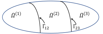
Fig. 6: Sample domain decomposed into three sub-regions.

In general, several regions might also meet at so-called corner vertices. The regions can now be used to split the composite matrix such that

(1) $${A}=\sum_{1\leq k\leq m}{A}^{(k)}$$

where

(2) $${A}^{(k)}_{ij}\neq 0\qquad\Rightarrow\qquad i,j\in S^{(k)}.$$

and

(3) $${A}^{(k)}_{ij}\neq 0\qquad\Rightarrow\qquad{A_{ij}}\neq 0.$$

Here, $S^{(k)}$ is the set of mesh nodes located within ${\Omega}^{(k)}$ (including those on the interface). While formally ${A}^{(k)}$ is $n\times n$, most rows are identically zero (i.e., rows not associated with $S_{k}$) and so the associated software would only store or compute on non-zero rows.

Mathematically, a region vector is an extended version of a composite vector that we express as

$$\llbracket{v}\rrbracket^{T}=\left[~{}\llbracket{v}\rrbracket_{1}^{T},~{}~{}~{}...,~{}~{}~{}\llbracket{v}\rrbracket_{m}^{T}~{}\right]^{T}$$

where double brackets denote regional representations, $v$ is the associated composite vector, and $\llbracket{v}\rrbracket_{k}$ is a sub-vector of $\llbracket{v}\rrbracket$ that consists of all degrees-of-freedom (dofs) that are co-located with the composite dofs given by $S^{(k)}$. We assume without loss of generality that region dofs within the same region are ordered consecutively (because region dofs can be ordered arbitrarily). As composite interface dofs reside within several regions, the vector $\llbracket{v}\rrbracket$ will be of length $n_{r}$ where $n_{r}\geq n$. If we consider a scalar problem and discrete representation of the example given in Figure 6, $\llbracket{v}\rrbracket$ consists of two dofs for each composite dof on $\mathrm{\Gamma}_{12}$ and $\mathrm{\Gamma}_{23}$.

A region framework can now be understood via a set of boolean transformation matrices. In particular, a composite vector must be transformed to a region vector where dofs associated with interfaces are replicated. To do this, consider an $n\times n_{r}$ boolean matrix that maps regional dofs to composite dofs. Specifically, a nonzero in the $i^{th}$ row and $j^{th}$ column implies that the $j^{th}$ regional unknown is co-located with the $i^{th}$ composite unknown. Each column of $\Psi$ has only one non-zero entry while the number of non-zeros in a row $i$ of $\Psi$ is equal to the number of regions that share the $i^{th}$ composite dof. Thus, a composite vector ${v}$ is mapped to a region vector $\llbracket{v}\rrbracket$ via $\llbracket{v}\rrbracket=\Psi^{T}{v}.$ The following properties are easily verified:

$\Psi\Psi^{T}$	is a diagonal matrix where the $(j,j)$ entry is the number of region dofs that are
	co-located with the $j^{th}$ composite dof;
$w=\Psi\llbracket{v}\rrbracket$	defines the $j^{th}$ element of $w$ as the sum of the co-located regional elements in
	$v$ associated with composite dof $j$;
$\llbracket{w}\rrbracket=\Psi^{T}\Psi\llbracket{v}\rrbracket$	defines the $j^{th}$ element of $w$ as the sum of the co-located regional elements in
	$v$ associated with regional dof $j$;
$w=(\Psi\Psi^{T})^{-1}\Psi\llbracket{v}\rrbracket$	defines the $j^{th}$ element of $w$ as the average of the co-located regional elements in
	$v$ associated with composite dof $j$;
$\llbracket{w}\rrbracket\hskip-2.8903pt=\hskip-2.8903pt\Psi^{T}(\Psi\Psi^{T})^{-1}\Psi\llbracket{v}\rrbracket$	defines the $j^{th}$ element of $w$ as the average of the co-located regional elements in
	$v$ associated with regional dof $j$.

Further, one can partition the columns of $\Psi$ in a region-wise fashion such that

(4) $$\Psi=\left[\Psi_{1},~{}~{}~{}...,~{}~{}~{}\Psi_{m}\right].$$

Thus, $\Psi_{k}^{T}$ maps composite dofs to only region $k$’s dofs, i.e., $\llbracket{v}\rrbracket_{k}=\Psi_{k}^{T}v$. The following additional properties hold:

$\Psi_{k}\Psi_{k}^{T}$	filters out dofs not associated with region $k$. In particular, $\Psi_{k}\Psi_{k}^{T}$ maps region
	vectors to new region vectors where the only nonzero matrix entries correspond
	to an identity block for dofs associated with region $k$;
$S=\Psi_{k}\Psi_{k}^{T}S$	if and only if $S$ only contains nonzeros in rows associated with region $k$;
$S=S\Psi_{k}\Psi_{k}^{T}$	if and only if $S$ only contains nonzeros in columns associated with region $k$;
$\Psi_{k}^{T}S\Psi_{k}$	is the submatrix of $S$ corresponding to the rows and columns of region $k$.

The boolean transformation matrices are not explicitly stored/manipulated in our software. Instead, functions are implemented to perform some of the properties listed above (e.g., averaging interface values).

A block diagonal region matrix can now be defined as

(5) $$\hskip 0.72229pt{\bf[\hskip-3.25201pt[\hskip-3.25201pt[}\hskip 0.72229pt{A}\hskip 0.72229pt{\bf]\hskip-3.25201pt]\hskip-3.25201pt]}\hskip 0.72229pt=\begin{pmatrix}\Psi_{1}^{T}A^{(1)}\Psi_{1}&&&&\cr&.&&&\cr&&.&&\cr&&&.&\cr&&&&\Psi_{m}^{T}A^{(m)}\Psi_{m}\end{pmatrix}.$$

Here, we employ a slightly different bracket symbol to emphasize that rows/columns associated with co-located dofs do not necessarily have the same values in this regional representation.

Lemma 1.

Let $\hskip 0.72229pt{\bf[\hskip-3.25201pt[\hskip-3.25201pt[}\hskip 0.72229pt{A}\hskip 0.72229pt{\bf]\hskip-3.25201pt]\hskip-3.25201pt]}\hskip 0.72229pt$ be defined by (5) and $\Psi$ be the boolean transformation matrix between region dofs and vector dofs. Then,

(6) $$\Psi\hskip 0.72229pt{\bf[\hskip-3.25201pt[\hskip-3.25201pt[}\hskip 0.72229pt{A}\hskip 0.72229pt{\bf]\hskip-3.25201pt]\hskip-3.25201pt]}\hskip 0.72229pt\Psi^{T}=A$$

when each split matrix $A^{(k)}$ only contains nonzeros in rows and columns associated with region $k$’s dofs.

Proof.

(7) $$\Psi\hskip 0.72229pt{\bf[\hskip-3.25201pt[\hskip-3.25201pt[}\hskip 0.72229pt{A}\hskip 0.72229pt{\bf]\hskip-3.25201pt]\hskip-3.25201pt]}\hskip 0.72229pt\Psi^{T} =\Psi_{1}\Psi_{1}^{T}A^{(1)}\Psi_{1}\Psi_{1}^{T}+...+\Psi_{m}\Psi_{m}^{T}A^{(m)}\Psi_{m}\Psi_{m}^{T}$$

(8) $$=A^{(1)}\Psi_{1}\Psi_{1}^{T}+...+A^{(m)}\Psi_{m}\Psi_{m}^{T}$$

(9) $$=A^{(1)}+...+A^{(m)}$$

(10) $$=A$$

where the simplifications to obtain (8) and (9) require that $A^{(k)}$ only have nonzeros in rows and columns associated with region $k$. ∎

To rewrite a multigrid V-cycle in a region oriented fashion, operations such as matrix-vector products must be performed with region matrices. For example, matrix-vector products with the discretization operator in the original multigrid cycle can instead be accomplished using (6). We also need to replace matrix-vector products associated with the grid transfers. For grid transfers, we prefer a different type of region matrix that we refer to as replicated interface matrices. Specifically, the replicated interface matrix for interpolation is defined by

(11) $$\llbracket{P}\rrbracket=\begin{pmatrix}\Psi_{1}^{T}P\mathrm{bar}{\Psi}_{1}&&&&\cr&.&&&\cr&&.&&\cr&&&.&\cr&&&&\Psi_{m}^{T}P\mathrm{bar}{\Psi}_{m}\end{pmatrix}$$

where $\mathrm{bar}{\Psi}$ is the boolean matrix associated with the regional to composite transformation on the coarse grid. Contrary to the standard region matrices, the composite operator (instead of split matrices) is injected to each of the regions. This implies that along the inter-region interfaces, matrix entries are replicated.

Lemma 2.

(12) $$\llbracket{P}\rrbracket\mathrm{bar}{\Psi}^{T}=\Psi^{T}P$$

when rows in the matrix $P$ do not contain nonzeros associated with multiple region interiors (i.e., non-interface dofs from multiple regions).

Proof.

(13) $$\llbracket{P}\rrbracket\mathrm{bar}{\Psi}^{T} =\begin{pmatrix}\Psi_{1}^{T}P\mathrm{bar}{\Psi}_{1}\mathrm{bar}{\Psi}_{1}^{T}\cr.\cr.\cr.\cr\Psi_{m}^{T}P\mathrm{bar}{\Psi}_{m}\mathrm{bar}{\Psi}_{m}^{T}\end{pmatrix}=\begin{pmatrix}\Psi_{1}^{T}P\cr.\cr.\cr.\cr\Psi_{m}^{T}P\end{pmatrix}=\Psi^{T}P$$

where we use the fact that the matrix $\Psi_{k}P$ only contains rows associated with region $k$ and that this submatrix contains only nonzeros in columns associated with region $k$ (under the assumption that $P$’s rows do not cross multiple region interiors). ∎

Lemma 3.

(14) $$\mathrm{bar}{\Psi}\llbracket{R}\rrbracket=R\Psi$$

when

(15) $$\llbracket{R}\rrbracket=\begin{pmatrix}\mathrm{bar}{\Psi}_{1}^{T}R\Psi_{1}&&&&\cr&.&&&\cr&&.&&\cr&&&.&\cr&&&&\mathrm{bar}{\Psi}_{m}^{T}R\Psi_{m}\end{pmatrix}$$

and $R$ contains no columns where the nonzeros are associated with multiple region interiors.

Proof.

Proof omitted as it is essentially identical to the proof for Lemma 2. ∎

Theorem 4.

$\mathrm{bar}{\Psi}\llbracket{R}\rrbracket\hskip 0.72229pt{\bf[\hskip-3.25201pt[\hskip-3.25201pt[}\hskip 0.72229pt{A}\hskip 0.72229pt{\bf]\hskip-3.25201pt]\hskip-3.25201pt]}\hskip 0.72229pt\llbracket{P}\rrbracket\mathrm{bar}{\Psi}^{T}=RAP$

Proof.

Follows as a direct result of applying (14), (12), and (6). ∎

Having established basic relationships between region and composite operations, we now re-formulate the multigrid algorithm primarily in terms of regional matrices and vectors. This re-formulation must be applied to both the multigrid setup phase and the multigrid cycle phase.

3.2 Multigrid Setup

The multigrid method requires that the discretization matrices, smoothers, and grid transfers be defined for all levels. For now, let us assume that we have $\Psi$ and $\hskip 0.72229pt{\bf[\hskip-3.25201pt[\hskip-3.25201pt[}\hskip 0.72229pt{A}\hskip 0.72229pt{\bf]\hskip-3.25201pt]\hskip-3.25201pt]}\hskip 0.72229pt$ on the finest level. For a two level multigrid method, we must define $\llbracket{P}\rrbracket,\llbracket{R}\rrbracket,\mathrm{bar}{\Psi},$ the regional coarse discretization operator $\llbracket{\mathrm{bar}{A}}\rrbracket$, and the region-based smoothers. For grid transfers, we directly create regional forms and never directly form the composite representation. That is, the composite $P$ and $R$ are only defined implicitly. In constructing region grid transfers, it is desirable to leverage standard structured mesh multigrid software (e.g., apply structured multigrid software to each region without knowledge of other regions). However, when creating the regional grid transfers, the implicitly defined composite interpolation must not contain any row where different nonzeros are associated with different region interiors. Further, stencils from different region blocks (of the block diagonal interpolation matrix) must be identical for co-located dofs. These requirements imply that fine interface vertices must interpolate only from coarse interface vertices and that interpolation coefficients for fine interface dofs have to be identical from neighboring regions. To satisfy these requirements, we use standard software in conjunction with some post-processing. In particular, the standard grid transfer algorithm must generate some coarse points on its region boundary (i.e., the interface) that can be used to fully interpolate to fine vertices on its region boundary. This is relatively natural for structured mesh multigrid software. It is also natural that interpolation stencils match along interfaces when using structured multigrid based on linear interpolation within neighboring regions. In this case, grid transfers can be constructed without any communication assuming that each processor owns one region. That is, each processor constructs the identical interpolation operator along the interface assuming that each processor has a copy of the coordinates and employs the same coarse grid points. However, if an algorithm is employed that does not produce identical interpolation coefficients from different regions, then a natural possibility would be to average the different interpolation stencils on a shared interface to redefine matching interpolation stencils at all co-located vertices. This averaging would incur some communication when each region is assigned to a different processor. This type of averaging might be employed if, for example, black box multigrid [8] is used to generate interpolation within each region as opposed to structured multigrid. In this way, the region interpolation algorithm will implicitly define a composite grid interpolation matrix that satisfies (11). Regional restriction matrices are obtained by taking the transpose of the regional interpolation matrices.

Coarse level discretizations can be constructed trivially. As indicated by Theorem 4, the regional coarse discretization is given by

(16) $$\llbracket{\mathrm{bar}{A}}\rrbracket=\llbracket{R}\rrbracket\hskip 0.72229pt{\bf[\hskip-3.25201pt[\hskip-3.25201pt[}\hskip 0.72229pt{A}\hskip 0.72229pt{\bf]\hskip-3.25201pt]\hskip-3.25201pt]}\hskip 0.72229pt\llbracket{P}\rrbracket,$$

which corresponds to performing a separate triple-matrix product for each diagonal block associated with each region. When a single region is owned by a single processor, no communication is needed in projecting the fine level regional discretization operator to the coarser levels. Given the major scaling challenges of these matrix-matrix operations within standard AMG algorithms, the importance of being able to perform this operation in a completely region-local fashion is significant. It should be noted, however, that a composite discretization matrix might be needed at the coarsest level for third-party software packages used to provide direct solvers or to further coarsen meshes in an unstructured AMG fashion. Of course, these composite matrices will only be needed at fairly coarse resolutions and they can be formed on the targeted level only (i.e., they do not have to be carried through all hierarchy levels). Thus, the costs associated with this construction via (6) should be modest.

To complete the multigrid setup, smoothers may require some setup phase. For Jacobi, Gauss–Seidel, and Chebyshev smoothing, the diagonal of the composite matrix must be computed during the setup phase. This is easily accomplished by storing the diagonal of the regional discretization matrix as a regional vector, e.g. $\llbracket{v}\rrbracket=diag(\llbracket{A}\rrbracket)$ using Matlab notation, and then simply applying the transformation, i.e., $\Psi^{T}\Psi\llbracket{v}\rrbracket$. For more sophisticated smoothers, it is natural to generate region analogs that are not completely equivalent to the composite versions. For example, one can generate region-local versions of Gauss–Seidel smoothers and Schwarz type methods where again $\Psi^{T}\Psi$ may be used to perform sums of nonzeros from different regions associated with co-located vertices. In this paper, we consider Jacobi, Gauss–Seidel, and Chebyshev smoothers. Some discussion of more sophisticated smoothers can be found in [3].

Finally, construction of a coarse level composite operator $\mathrm{bar}{A}$ is also trivial. In particular, $\mathrm{bar}{\Psi}$ is just the submatrix of $\Psi$ corresponding to taking rows associated with coarse composite vertices and columns associated with the co-located coarse region vertices. Thus, it is convenient if the interpolation algorithm also provides a list of coarse vertices, though this can be deduced from the interpolation matrix (i.e., the vertices associated with rows containing only one nonzero).

Having computed the coarse level operator $\llbracket{\mathrm{bar}{A}}\rrbracket$ via the recursive application of (16), its composite representation is given as

(17) $$\mathrm{bar}{A}=\mathrm{bar}{\Psi}\llbracket{\mathrm{bar}{A}}\rrbracket.$$

This corresponds to forming sums of matrix rows that correspond to co-located nodes on region interfaces.

3.3 Multigrid Cycle

The multigrid cycle consists primarily of residual calculations, restriction, interpolation, and smoother applications. The composite residual can be calculated with region matrices via

(18) $$r=b-Au=b-\Psi\hskip 0.72229pt{\bf[\hskip-3.25201pt[\hskip-3.25201pt[}\hskip 0.72229pt{A}\hskip 0.72229pt{\bf]\hskip-3.25201pt]\hskip-3.25201pt]}\hskip 0.72229pt\Psi^{T}u.$$

Normally, however, one seeks to compute the regional form of the residual using regional representations of $b$ and $u$ via

(19) $$\llbracket{r}\rrbracket=\llbracket{b}\rrbracket-\Psi^{T}\Psi\hskip 0.72229pt{\bf[\hskip-3.25201pt[\hskip-3.25201pt[}\hskip 0.72229pt{A}\hskip 0.72229pt{\bf]\hskip-3.25201pt]\hskip-3.25201pt]}\hskip 0.72229pt\llbracket{u}\rrbracket,$$

which is derived by pre-multiplying (18) by $\Psi^{T}$ and recognizing that $\llbracket{r}\rrbracket=\Psi^{T}r,\llbracket{b}\rrbracket=\Psi^{T}b,$ and $\llbracket{u}\rrbracket=\Psi^{T}u$. Thus, the only difference with a standard residual calculation is the interface summation given by $\Psi^{T}\Psi$. For interpolation, we seek the regional version of interpolation

(20) $$\llbracket{w}\rrbracket =\Psi^{T}Pv$$

(21) $$=\llbracket{P}\rrbracket\mathrm{bar}{\Psi}^{T}v$$

(22) $$=\llbracket{P}\rrbracket\llbracket{v}\rrbracket$$

where we used Lemma 2 to simplify the interpolation expression. Thus, the interpolation matrix-vector product is identical to a standard matrix-vector product, incurring no inter-region communication.

The region version of the restriction matrix-vector product is a bit more complicated. We begin by observing that

(23) $$R =\mathrm{bar}{\Psi}\llbracket{R}\rrbracket\Psi^{T}(\Psi\Psi^{T})^{-1}$$

(24) $$=\mathrm{bar}{\Psi}\llbracket{R}\rrbracket\llbracket{\Psi\Psi^{T}}\rrbracket^{-1}\Psi^{T}.$$

Lemma 3 can be used to verify (23). For (24), we define an interface version of $\Psi\Psi^{T}$ analogous to (11) and (15). Specifically, the $\llbracket{\Psi\Psi^{T}}\rrbracket$ matrix is both diagonal and block diagonal where the $k^{th}$ block is given by $\Psi_{k}^{T}(\Psi\Psi^{T})\Psi_{k}$. By employing a commuting relationship (whose proof is omitted as it closely resembles that of Lemma 2), one arrives at (24). Finally, pre-multiplying $w=Rv$ by $\mathrm{bar}{\Psi}^{T}$, substituting (24) for $R$, and recognizing that $\llbracket{w}\rrbracket=\Psi^{T}w$ and $\llbracket{v}\rrbracket=\Psi^{T}v$, it can be shown that the desired matrix-vector product relationship is given by

$$\llbracket{w}\rrbracket=\mathrm{bar}{\Psi}^{T}\mathrm{bar}{\Psi}\llbracket{R}\rrbracket\llbracket{\Psi\Psi^{T}}\rrbracket^{-1}\llbracket{v}\rrbracket.$$

Thus, the restriction matrix-vector product corresponds to region-local scaling, followed by a region-local matrix-vector product followed by summation of co-located regional quantities.

3.4 Region level smoothers

Jacobi smoothing is given by

$$\llbracket{u}\rrbracket\leftarrow\llbracket{u}\rrbracket+\omega~{}\llbracket{\tilde{D}^{-1}}\rrbracket\llbracket{r}\rrbracket$$

with $\llbracket{r}\rrbracket$ computed via (19), $\omega$ is a damping parameter, and $\llbracket{\tilde{D}}\rrbracket$ is the diagonal of the composite operator ${A}$ stored in regional form (as discussed in Section 3.2).

Implementation of a classic Gauss–Seidel algorithm always requires some care on parallel computers, even when using standard composite operators. Though a high degree of concurrency is possible with multi-color versions, these are difficult to develop efficiently and require communication exchanges for each color on message passing architectures. Instead, it is logical to adapt region Gauss–Seidel using domain decomposition ideas (as is typically done for composite operators as well). The $K$ sweep Gauss–Seidel smoother is summarized in Algorithm 1.

0:  $\omega,\llbracket{A}\rrbracket,\llbracket{b}\rrbracket,\llbracket{\tilde{D}}\rrbracket,\llbracket{u}\rrbracket$

  for $k=0,\ldots,K-1$ do

     $\llbracket{\delta}\rrbracket=0$

     compute $\llbracket{r}\rrbracket$ via (19)

     // for each region …

     for $\ell=1,\ldots,m$  do

        for $i=0,\ldots,N^{(\ell)}$ do

           $r^{(\ell)}_{i}=r^{(\ell)}_{i}=-\Sigma_{j}A^{(\ell)}_{ij}\delta^{(\ell)}_{j}$

           $\delta^{(\ell)}_{i}=\omega r^{(\ell)}_{i}/\tilde{d}^{(\ell)}_{ii}$

           $u^{(\ell)}_{i}=u^{(\ell)}_{i}+\delta^{(\ell)}_{i}$

Algorithm 1 Gauss–Seidel smoother for region-type problems

Here, the notation $r^{(\ell)}_{i}$ refers to the $i^{th}$ component of the $\ell^{th}$ region’s vector while $A^{(\ell)}_{ij}$ refers to a particular nonzero in region $\ell$’s matrix. The intermediate quantity $\delta^{(\ell)}_{i}$ is used to update the local solution and the local residual. Notice that the only communication is embedded within the residual calculation at the top of the outer loop. This low communication version of the algorithm differs from true Gauss–Seidel in that a region’s updated residual only takes into account solution changes within the region. This means that solution values along a shared interface are not guaranteed to coincide during this state of the algorithm.

Chebyshev smoothing relies on optimal Chebyshev polynomials tailored to reduce errors within the eigenvalue interval $\lambda_{i}\in[\lambda_{\mathrm{min}},\lambda_{\mathrm{max}}]$ with $\lambda_{\mathrm{min}}$ and $\lambda_{\mathrm{max}}$ denoting the smallest and largest eigenvalue of interest of the operator $\llbracket{A}\rrbracket$. The largest eigenvalue is obtained by a few iterations of the power method. Following the Chebyshev implementation in Ifpack2 [19], we approximate this interval by $[\lambda_{\mathrm{min}},\lambda_{\mathrm{max}}]\approx[\alpha,\beta]$ with $\alpha=\tilde{\lambda}_{\mathrm{max}}/\eta$ and $\beta=\kappa\tilde{\lambda}_{\mathrm{max}}$ where $\tilde{\lambda}_{\mathrm{max}}$ is the estimate obtained via the power method,  $\eta$ denotes a ratio that is either user supplied or given by the coarsening rate between levels (defaulting to $\eta=20$) and $\kappa$ is the so-called “boost factor” (often defaulting to $\kappa=1.1$). The Chebyshev smoother up to polynomial degree $K$ is summarized in Algorithm 2.

0:  $\theta=\frac{\alpha+\beta}{2},\delta=\frac{2}{\beta-\alpha},\llbracket{A}\rrbracket,\llbracket{\tilde{D}}\rrbracket,\llbracket{u}\rrbracket,\llbracket{r}\rrbracket$

  $\rho=\left(\theta\delta\right)^{-1}$

  $\llbracket{d}\rrbracket=\frac{1}{\theta}\delta\llbracket{\tilde{D}^{-1}}\rrbracket\llbracket{r}\rrbracket$

  for $k=0,\ldots,K$ do

     $\llbracket{u}\rrbracket=\llbracket{u}\rrbracket+\llbracket{d}\rrbracket$

     compute $\llbracket{r}\rrbracket$ via (19)

     $\rho_{\mathrm{old}}=\rho$

     $\rho=\left(2\theta\delta-\rho_{\mathrm{old}}\right)^{-1}$

     $\llbracket{d}\rrbracket=\rho\rho_{\mathrm{old}}\llbracket{d}\rrbracket+2\rho\delta\llbracket{\tilde{D}^{-1}}\rrbracket\llbracket{r}\rrbracket$

Algorithm 2 Chebyshev smoother for region-type problems

3.5 Coarse level solver

The region hierarchy consists of $L_{\mathrm{r}}$ levels $\ell\in\{0,\ldots,L_{\mathrm{r}}-1\}$. Having computed the coarse composite operator $\mathrm{bar}{A}$ via (17) on level $L_{\mathrm{r}}-1$, we construct a coarse level solver for the region MG hierarchy. We explore two options:

• Direct solver: If tractable, a direct solver relying on the factorization $\mathrm{bar}{A}=\mathrm{bar}{L}\mathrm{bar}{U}$ is constructed. As usual, its applicability and performance (especially w.r.t. setup time) largely depend on the number of unknowns on the coarse level.

• AMG V-cycle: If $\mathrm{bar}{A}$ is too large to be tackled by a direct solver, one can construct a standard AMG hierarchy with an additional $L_{\mathrm{c}}$ levels. The coarse level solve of the region MG cycle is then replaced by a single V-cycle using (SA-)AMG [24]. This AMG hierarchy requires only the operator $\mathrm{bar}{A}$ and its nullspace, which can be extracted from the region hierarchy. The AMG V-cycle itself will create as many levels as needed, such that its coarsest level can be addressed using a direct solver. The number of additional levels for the AMG V-cycle is denoted by $L_{\mathrm{c}}$. For efficiency, load re-balancing is crucial. (Note that the total number of levels is now $L=L_{\mathrm{r}}+L_{\mathrm{c}}-1$, where the subtraction by one reflects the change of data layout from region to composite format without coarsening.)

The latter option is also of interest for problems, where the regional fine mesh has been constructed through regular refinement of an unstructured mesh. Here, the region MG scheme can only coarsen until the original unstructured mesh is recovered. AMG has to be used for further coarsening. Assuming one MPI rank per region, i.e. one MPI rank per element in the initial unstructured mesh, the need for re-balancing (or even multiple re-balancing operations throughout the AMG hierarchy) becomes obvious.

3.6 Regional multigrid summary

To summarize, the mathematical foundation and exact equivalence with standard composite grid multigrid requires that

1. the composite matrix be split according to (1) such that each piece only includes nonzeros defined on its corresponding region;

2. each row (column) of the composite interpolation (restriction) matrix cannot include nonzeros associated with multiple region interiors;

Thus, co-located fine interpolation rows consist only of nonzeros associated with coarse co-located vertices. Likewise, co-located coarse restriction columns only include nonzeros associated with fine co-located vertices. Finally, the grid transfer condition implies that regional forms of interpolation (restriction) must have matching rows (columns) associated with co-located dofs. It is important to notice that if the region interfaces are not curved or jagged and if linear interpolation is used to define the grid transfer along region interfaces (where fine interface points only interpolate from coarse points on the same interface), then each region’s block of the block interpolation operator can be defined independently as long as the selection of coarse points on the interface match. That is, the resulting region interpolation operator will satisfy the Lemma conditions without the need for any communication. If, however, a more algebraic scheme is used to generate the inter-grid transfers, then some communication might be needed to ensure that the interpolation operators satisfy the Lemma conditions at the interface. This would be true if a black box multigrid [8] is used to define the grid transfers or if a more general algebraic multigrid scheme such as smoothed aggregation [24] is used to define grid transfers. This is discussed further in Section 5.

Figure 7 summarizes the regional version of the two level algorithm.

$\text{function}\;\textsf{mgSetup}(\hskip 0.72229pt{\bf[\hskip-3.25201pt[\hskip-3.25201pt[}\hskip 0.72229pt{A}\hskip 0.72229pt{\bf]\hskip-3.25201pt]\hskip-3.25201pt]}\hskip 0.72229pt)$		$\text{function}\;\textsf{mgCycle}(\hskip 0.72229pt{\bf[\hskip-3.25201pt[\hskip-3.25201pt[}\hskip 0.72229pt{A}\hskip 0.72229pt{\bf]\hskip-3.25201pt]\hskip-3.25201pt]}\hskip 0.72229pt,\llbracket{u}\rrbracket,\llbracket{b}\rrbracket):$
	$\llbracket{D}\rrbracket\leftarrow\textsf{diag}(\Psi^{T}\Psi~{}\textsf{diag}(\hskip 0.72229pt{\bf[\hskip-3.25201pt[\hskip-3.25201pt[}\hskip 0.72229pt{A}\hskip 0.72229pt{\bf]\hskip-3.25201pt]\hskip-3.25201pt]}\hskip 0.72229pt))$		$\llbracket{u}\rrbracket\leftarrow\textsf{applySmoother}(\llbracket{u}\rrbracket,\llbracket{b}\rrbracket,\hskip 0.72229pt{\bf[\hskip-3.25201pt[\hskip-3.25201pt[}\hskip 0.72229pt{A}\hskip 0.72229pt{\bf]\hskip-3.25201pt]\hskip-3.25201pt]}\hskip 0.72229pt)$
	$\llbracket{P}\rrbracket\leftarrow\textsf{construct}P(\hskip 0.72229pt{\bf[\hskip-3.25201pt[\hskip-3.25201pt[}\hskip 0.72229pt{A}\hskip 0.72229pt{\bf]\hskip-3.25201pt]\hskip-3.25201pt]}\hskip 0.72229pt)$		$\llbracket{r}\rrbracket\leftarrow\llbracket{b}\rrbracket-\Psi^{T}\Psi\hskip 0.72229pt{\bf[\hskip-3.25201pt[\hskip-3.25201pt[}\hskip 0.72229pt{A}\hskip 0.72229pt{\bf]\hskip-3.25201pt]\hskip-3.25201pt]}\hskip 0.72229pt\llbracket{u}\rrbracket$
	$\llbracket{R}\rrbracket\leftarrow\llbracket{P}\rrbracket^{T}$		$\llbracket{\mathrm{bar}{u}}\rrbracket\leftarrow 0$
	${\hskip 0.72229pt{\bf[\hskip-3.25201pt[\hskip-3.25201pt[}\hskip 0.72229pt{\mathrm{bar}{A}}\hskip 0.72229pt{\bf]\hskip-3.25201pt]\hskip-3.25201pt]}\hskip 0.72229pt}\leftarrow\llbracket{R}\rrbracket\hskip 0.72229pt{\bf[\hskip-3.25201pt[\hskip-3.25201pt[}\hskip 0.72229pt{A}\hskip 0.72229pt{\bf]\hskip-3.25201pt]\hskip-3.25201pt]}\hskip 0.72229pt\llbracket{P}\rrbracket$		$\llbracket{\mathrm{bar}{u}}\rrbracket\leftarrow\textsf{solve}(\hskip 0.72229pt{\bf[\hskip-3.25201pt[\hskip-3.25201pt[}\hskip 0.72229pt{\mathrm{bar}{A}}\hskip 0.72229pt{\bf]\hskip-3.25201pt]\hskip-3.25201pt]}\hskip 0.72229pt,\llbracket{\mathrm{bar}{u}}\rrbracket,\mathrm{bar}{\Psi}^{T}\mathrm{bar}{\Psi}\llbracket{R}\rrbracket\llbracket{\Psi\Psi^{T}}\rrbracket^{-1}\llbracket{r}\rrbracket)$
	$\mathrm{bar}{\Psi}\leftarrow\textsf{inject}(\Psi)$		$\llbracket{u}\rrbracket\leftarrow\llbracket{u}\rrbracket+\llbracket{P}\rrbracket\llbracket{\mathrm{bar}{u}}\rrbracket$

Fig. 7: Two level regional multigrid for the solution of ${A}\,{u}=\,{b}$.

Besides the $\textsf{inject}()$ operation, the only possible difference during setup is a small modification of $\textsf{construct}P()$ that may be necessary to ensure that interpolation stencils match at co-located vertices. In $\textsf{applySmoother}()$, any region level smoother from Section 3.4 is applied. The main difference in the $\textsf{solve}()$ phase is the scaling $\llbracket{\Psi\Psi^{T}}\rrbracket^{-1}$, the interface summation $\Psi^{T}\Psi$, and possibly the need to convert between regional and composite forms if third party software is employed at sufficiently coarse levels.

4 Non-invasive construction of region application operators

To this point, we have assumed that $\Psi$ and $\hskip 0.72229pt{\bf[\hskip-3.25201pt[\hskip-3.25201pt[}\hskip 0.72229pt{A}\hskip 0.72229pt{\bf]\hskip-3.25201pt]\hskip-3.25201pt]}\hskip 0.72229pt$ on the finest level are available. However, most finite element software is not organized to generate these. Our goal is to limit the burden on application developers by instead employing a fully assembled discretization or composite matrix on the finest level. In this section, we first describe the application information that we require to generate $\Psi$. Then, we describe an automatic matrix splitting or dis-assembly process so that our software can generate $\hskip 0.72229pt{\bf[\hskip-3.25201pt[\hskip-3.25201pt[}\hskip 0.72229pt{A}\hskip 0.72229pt{\bf]\hskip-3.25201pt]\hskip-3.25201pt]}\hskip 0.72229pt$, effectively via (5).

In addition to fairly standard distributed matrix requirements (e.g., each processor supplies a subset of owned matrix rows and a mapping between local and global indices for the owned rows), applications must provide information to construct $\Psi$ and to facilitate fast kernels. Specifically, applications furnish a region id and the number of grid points in each dimension for regions owned by a processor. As noted, our software is currently limited in that each processor owns one entire region. However, we will keep the discussion general.

The main additional requirement is a description of the mesh at the region interfaces. In particular, it must be known, to which region(s) each node belongs. If a node is a region-internal node, it only belongs to one region. If it resides on a region interface, it belongs to multiple regions. Note that the number of associated regions depends on the spatial dimension, the location within the mesh, and the region topology. For example, nodes on inter-region faces (not also on edges and corners), edges (not also on corners), and corners belong to 2 regions, 4 regions, and 8 regions respectively for a three-dimensional problem with cartesian-type cuboid regions. Figure 8 gives a concrete two region example in a two-dimensional setting. In this example, one processor owns the entire $5\times 3$ topmost rectangular region while another processor owns the bottom most $3\times 2$ rectangular region.

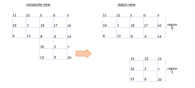
Fig. 8: Sample user-provided mapping of mesh nodes to regions.

The mapping for this example looks as follows:

• Nodes $0,1,3,4,5,10,11,12,14,15,17,18,19$ reside in region ${\Omega}^{(0)}$.

• Nodes $2,7,9,13,16,20$ reside in region ${\Omega}^{(1)}$.

• Nodes $6,8,14$ are located on the region interface and belong to both regions ${\Omega}^{(0)}$ and ${\Omega}^{(1)}$.

Based on this user-provided mapping data, we can now “duplicate” interface nodes and assign unique GIDs for all replicated interface nodes and their associated degrees of freedom. The right-hand side sketch in Figure 8 illustrates a computed mapping of global composite ids to the global region layout ids. Notice that the only global ids to change are the composite ghost ids. Specifically, new global ids are assigned by the framework to the ghosts associated with the bottom processor so that each of the unknowns along a shared interface has a unique global id. The overall structured framework can be setup based on this user-supplied mapping and effectively build the $\Psi$ operator. Of course, we do not explicitly form $\Psi$, but build data structures and functions to perform the necessary operations associated with $\Psi$.

To apply (5), the composite matrix must first be split so that (1), (2) and (3) are satisfied. Mathematically, matrix entries associated with co-located vertices must be split or divided between different terms in the summation. In this paper, we scale any off-diagonal matrix entries by the number of regions that share the same edge. Formally, scaled entries correspond to $A_{ij}\neq 0$ such that there exist exactly $q~{}(\geq 2)~{}\Psi_{k}$’s with a nonzero in the $i^{th}$ and $j^{th}$ rows. If we denote these $\Psi_{k}$’s by $\Psi_{k_{1}},\Psi_{k_{2}},...,\Psi_{k_{q}}$, then

$$A_{ij}^{(k_{1})}=A_{ij}^{(k_{2})}=...=A_{ij}^{(k_{q})}=A_{ij}/q.$$

The matrix diagonal is then scaled so that the row sum of each region matrix is identically zero. With $\Psi$ and the splitting choice specified, the entire multigrid cycle is now defined. Though this splitting choice is relatively simple, it has no numerical impact when geometric grid transfers are employed in conjunction with a Jacobi smoother. However, some multigrid components such as region-oriented smoothers (e.g., region-local Gauss–Seidel) and matrix-dependent algorithms for generating grid transfers (e.g., black-box multigrid) are affected by the splitting choice. We simply remark that we have experimented with a variety of scalar PDEs using black-box multigrid, and this splitting choice generally leads to multigrid convergence rates that are similar to conventional multigrid algorithms applied to composite problems.

While we do not provide the implementation details associated with computations such as $\Psi_{k}^{T}A^{(k)}\Psi_{k}$ and the conversions between regional and composite vectors, it is worth pointing out that some implementation aspects can leverage ghosting and overlapping Schwarz capabilities found in many iterative solver frameworks. In our case, some of these operations can be performed in a relatively straight-forward fashion using Trilinos’ import/export mechanism. The import feature is most commonly used in Trilinos to perform operations such a matrix-vector products. An import can be used to take vectors without ghost unknowns and create a new vector with ghost unknowns obtained from neighboring processors. This standard import operation is similar to transforming a composite vector to a region vector. The main difference is that only some ghost unknowns (those that correspond to a shared interface) need to be obtained from neighboring processors.

The import facility is fairly general in that it can also be used to replicate matrix rows needed within a standard overlapping Schwarz preconditioner. In this case, import takes a non-overlapped matrix where each matrix row resides on only one processor and creates an overlapped matrix, where some matrix rows are duplicated and reside within more than one sub-domain. When an overlap of one is used, each processor receives a duplicate row for each of its ghost unknowns. This is similar to the process of generating regional matrices from composite matrices (only requiring rows from a subset of ghosts). Once matrix rows (corresponding to interfaces) have been replicated, they must be modified to satisfy (1). In particular, any column entries (within interface rows) that correspond to connections with neighboring regions must be removed. Further, entries that have been replicated along the interface must be scaled in a post-processing step.

In a standard Schwarz preconditioner, solutions obtained on each sub-domain must be combined. That is, overlapped solution values must be combined (e.g., averaged) to define a unique non-overlapping solution. For this mapping from overlapped to non-overlapped, Trilinos contains an export mechanism. This export allows for different type of operations (e.g., averages or sums) to be used when combining multiple entries associated with the same non-overlapped unknown. This is similar to transforming regional vectors to composite vectors. One somewhat subtle issue is that the unique region global ids presented in Figure 8 are not needed in an overlapping Schwarz capability, but are needed for the region-multigrid framework to perform further operations on the region-layout systems. Thus, the conversions between composite and regional forms has been implemented in two steps. The first step closely resembles the Schwarz process and corresponds to the movement of data between overlapped and non-overlapped representations as just discussed, but without introducing the new global ids. The second step then defines the new global ids to complete the conversion process.

5 Structured/unstructured mesh hybrid

We now discuss the adaptation of regional multigrid to the case where some unstructured regions are introduced into the grid. As the mathematical foundation presented earlier makes no assumptions on grid structure, the requirements summarized in Section 3.6 still hold. The unstructured regions do not introduce software modifications associated with satisfying the matrix splitting or dis-assembly requirements. However, grid transfer construction requires some care. In particular, some pre- and post-processing modifications are needed for the AMG algorithm that constructs regional grid transfers within the unstructured regions. No additional modifications are needed to produce structured grid multigrid transfers within the structured regions.

Figure 9 provides a simple illustration of an unstructured triangular region attached to a $7\times 7$ structured region. In Figure 9 a subset of vertices are labelled with a ‘c’ to denote a possible choice of coarse points denoted as Cpts. The Cpts set refers to a subset of fine mesh vertices that are chosen by a classical AMG algorithm to define the mesh vertices of the coarse mesh.

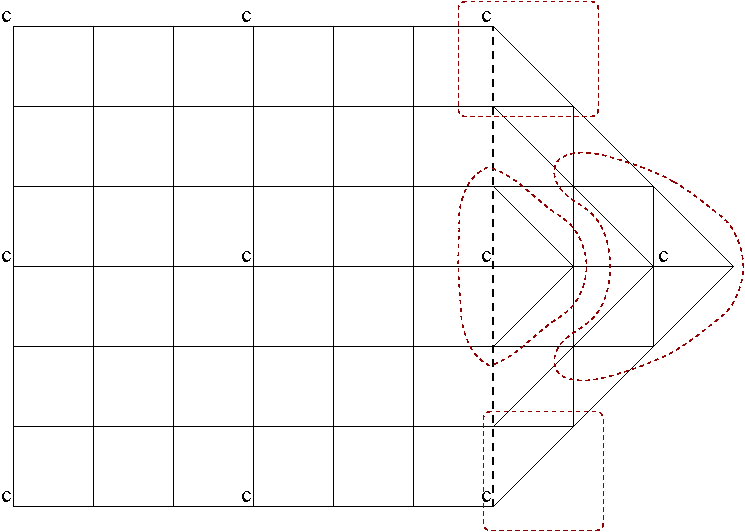
Fig. 9: Structured square region attached to an unstructured triangular region. The structure/unstructured interface is given by a dark dashed line. A c denotes the location of a Cpt. Red dashed lines encircle unstructured aggregates.

Notice that within structured regions, the Cpts have been defined in a standard structured fashion. Ideally, it would be attractive to apply a standard AMG algorithm with no software modifications to coarsen and define grid transfers for unstructured regions. However, the resulting grid transfers stencils at co-located vertices must match their structured region counter-parts. This means that the same set of three Cpts should be chosen by the structured algorithm and the unstructured algorithm along the interface in our Figure 9 example and that the interpolation coefficients along the interface be chosen in a very specific way.

In this paper, we do not employ classical AMG for unstructured regions, but instead use the simpler plain aggregation variant of smoothed aggregation AMG method (SA) [24]. With both smoothed aggregation and plain aggregation multigrid, the coarsening procedure is the same. In particular, coarsening is performed by aggregating together sets of fine vertices as opposed to identifying Cpts. Each aggregate is essentially formed by choosing a root vertex and including all of the root’s neighbors that have not already been included in another aggregate. Loosely, one can think of the aggregate root point as a Cpt. In Figure 9, four aggregates in the unstructured region are depicted with dashed red lines. To enforce the consistency of the Cpts choice at the interface, the unstructured aggregation software must be changed so that it initially chooses root points and aggregates associated with structured coarsening. In our standard coarsening software, aggregation occurs in stages that are pipelined together. Each stage applies a specific algorithm that might only aggregate a subset of fine mesh vertices and then pass the partially-aggregated mesh to the next stage (that attempts to add more aggregates). Staging is a practical way to combine different aggregation algorithms with different objectives to ensure that all mesh vertices are eventually aggregated. To accommodate structured/unstructured interfaces, a new aggregation stage was devised to start the aggregation process. This new stage only aggregates vertices on interfaces and chooses root nodes in a structured fashion (employing a user-defined coarsening rate). Aggregates are chosen so that no interface vertices remain unaggregated after this stage. Once this new stage completes, the standard unstructured aggregation stages can proceed without further modification. Notice that coarsening of structured and unstructured regions can proceed fully in parallel (with no need for communication between the regions) as processors responsible for unstructured regions redundantly coarsen/aggregate the interface using the new devised aggregation stage while structured regions also coarsen the interface using a standard structured coarsening scheme. Since both structured and unstructured regions employ structured aggregation along the mesh interface, matching Cpts are guaranteed.

Not only should coarsening be consistent along interfaces, but interpolation coefficients at co-located vertices should match those produced by the structured regions. For plain aggregation, multigrid this will be the case as long as the structured region grid transfers use the same methodology of piecewise constant basis functions. Specifically, the corresponding plain aggregation interpolation basis functions are just piecewise constants for most applications. As the plain aggregation basis functions do not rely on the coefficients of the discretization matrix, each region’s version of an interpolation stencil for a common interface will coincide exactly in the plane aggregation case. This will not generally be true for more sophisticated AMG schemes such as smoothed aggregation where the interpolation coefficients depend on the discretization matrix coefficients. Effectively, a different algorithm is used to generate the interpolation coefficients and so there is no reason why interpolation stencils should match those produced with linear interpolation. In this paper, we avoid this issue by only considering plain aggregation AMG for unstructured regions in conjunction with piecewise constant interpolation (as opposed to linear interpolation) for structured regions. However, we have identified two relatively straight-forward options both involving some form of post-processing to the grid transfer operators. One possibility is that a subset of processors communicate/coordinate with each other to arrive at one common interpolation stencil for each unknown on a shared interface. Obviously, this requires communication and is somewhat tedious to implement. The second possibility is that linear basis functions always define interpolation along interfaces between structured and unstructured regions. In this case, communication can be avoided by employing a post-processing procedure within the unstructured grid transfer algorithm to calculate (and overwrite) the appropriate interpolation operator along its interfaces. We omit the details but indicate that all the required information (coarse grid point locations and fine grid point locations) is already available within our software framework.

To complete the discussion, we highlight some implementation aspects associated with incorporating these pre- and post-processing changes into a code such as MueLu which is based on a factory design, where different classes must interact with different objects (e.g., aggregates, grid transfer matrices) needed to construct the multigrid hierarchy. In particular, parameter lists are used to enter algorithm choices and application specific data. In our context, the application must indicate the following for each processor via parameter list entries:

• whether or not it owns a structured region or an unstructured region

• the dimensions and coarsening rate for processors owning structured regions

• the dimensions and coarsening rate of each neighboring structured region for processors owning unstructured regions

Further, processors owning unstructured regions, that border structured regions, must still provide structured region information for structured interfaces. This includes a list of neighboring regions and the mapping of mesh nodes to regions as introduced in Figure 8.

With the proper user-supplied information, MueLu assigns a hybrid factory to address the prolongators. This hybrid factory includes an internal switch to then invoke either a structured region grid transfer factory or an unstructured region grid transfer factory. The hybrid factory essentially creates the grid transfer matrix object, allowing the sub-factories to then populate this matrix object with suitable entries. It is this hybrid factory that invokes the aggregation process that starts with the interface aggregation stage for unstructured regions. It is also responsible for the post-processing (i.e., the updating of the prolongator matrix rows corresponding to interface rows) for the unstructured regions. In this way, the standard structured factories and standard unstructured factories require virtually no modifications, as these are mostly confined to the hybrid factory. More information about MueLu’s factory design can be found in [6].

6 Numerical Results

Computational experiments are performed to highlight the equivalence between MG cycles employing either composite operators or region operators as described by the Lemmas/Theorems presented earlier. This is followed by experiments to illustrate performance benefits of structured MG. Finally, we conclude this section with an investigation demonstrating a structured region approach that also incorporates a few unstructured sub-domains. All the experiments that follow can be reproduced using Trilinos at commit 86095f3d93e.

6.1 Region MG Equivalence

To assess the equivalence of structured region MG to standard structured MG (without regions and region interfaces), we study a two-dimensional Laplace problem discretized with a $7$-point stencil on two different meshes, a square $730\times 730$ mesh and a rectangular $700\times 720$ mesh. The problem is run on $9$ MPI ranks for the region solver and run in serial for standard structured MG. Here, we employ MG as a solver (not as a preconditioner within a Krylov method), and the iteration is terminated when the relative residual drops below $10^{-12}$.

The structured MG scheme employs a standard fully assembled matrix (i.e., a composite matrix in this paper’s terminology). It uses a coarsening rate of $3$ in each coordinate direction and linear interpolation defines the grid transfer. The multigrid hierarchy consists of $4$ levels. Specifically, the hierarchy mesh sizes from finest to coarsest for the square mesh are $730\times 730$, $244\times 244$, $82\times 82$, and $28\times 28$. Notice that all of these meshes correspond to $3^{k}+1$ points in each coordinate direction. Our software does not require these specific mesh sizes, but this is needed to demonstrate exact equivalence. That is, both the composite MG and the region MG must coarsen identically. For the rectangular mesh, sizes are not chosen so that the coarsening is identical (i.e., the number of vertices in each mesh dimension do not correspond to $3^{k}+1$). Thus, we expect some small residual history differences for the rectangular mesh. Fully structured multigrid is implemented in Trilinos/MueLu using an option referred to as structured uncoupled aggregation. For the region MG hierarchy on the other hand, the mesh is partitioned into $9~{}(=3\times 3)$ regions, where each region is assigned to one MPI rank. In this case, the square domain multigrid hierarchy for each processor’s sub-mesh or region mesh is $244\times 244$, $82\times 82$, $28\times 28$, and $9\times 9$. In each coordinate direction, the overall finest mesh appears to have $732~{}(=3$ processors $~{}\times~{}244$ per processor) mesh points, which is not equal to the $730$ mesh points used for the fully structured composite MG cycle. However, one must keep in mind that 2 vertices are replicated along a mesh line in a coordinate direction (due to region the interfaces). Again, these carefully chosen sizes are to enforce an identical coarsening procedure for the two MG solvers (and thus satisfy the conditions of the Lemmas/Theorems presented earlier), as opposed to a hard requirement of the software. The region multigrid method also uses a structured aggregation option to implement this type of structured coarsening.

Table 1

Table 1: Residual histories to study the equivalence of the structured region MG scheme to a classical structured MG

	Jacobi		Gauss–Seidel		Chebyshev
$\#$its.	Structured	$9$ Regions	Structured	$9$ Region	Structured	$9$ Regions
0	1.00000000e+00	1.00000000e+00	1.00000000e+00	1.00000000e+00	1.00000000e+00	1.00000000e+00
1	1.77885821e-02	1.77885821e-02	1.34144214e-02	1.34395087e-02	1.42870540e-02	1.42868592e-02
2	3.09066249e-03	3.09066249e-03	1.22727384e-03	1.23709339e-03	9.93752447e-04	9.93713870e-04
3	6.17432509e-04	6.17432509e-04	1.27481334e-04	1.29627870e-04	1.21921975e-04	1.21914771e-04
4	1.29973612e-04	1.29973612e-04	1.41133381e-05	1.45165400e-05	1.58413729e-05	1.58401012e-05
5	2.81812370e-05	2.81812370e-05	1.61878817e-06	1.69088891e-06	2.11105538e-06	2.11083642e-06
6	6.22574415e-06	6.22574415e-06	1.89847271e-07	2.02561731e-07	2.86037857e-07	2.86000509e-07
7	1.39312700e-06	1.39312700e-06	2.26276959e-08	2.48757453e-08	3.92564304e-08	3.92500462e-08
8	3.14666393e-07	3.14666393e-07	2.73250326e-09	3.13452182e-09	5.44989750e-09	5.44879379e-09
9	7.15836477e-08	7.15836477e-08	3.33798476e-10	4.06768456e-10	7.65555357e-10	7.65361045e-10
10	1.63770972e-08	1.63770972e-08	4.12201997e-11	5.46524944e-11	1.08974518e-10	1.08939546e-10
11	3.76413472e-09	3.76413472e-09	5.14512205e-12	7.64221900e-12	1.57581213e-11	1.57516868e-11
12	8.68493274e-10	8.68493274e-10	6.49387222e-13	1.11538919e-12	2.32197807e-12	2.32077246e-12
13	2.01044350e-10	2.01044350e-10		1.69735837e-13	3.49742848e-13	3.49514354e-13
14	4.66714466e-11	4.66714466e-11
15	1.08616953e-11	1.08616953e-11
16	2.53347464e-12	2.53347464e-12
17	5.92132868e-13	5.92132868e-13

(a) $730\times 730$ square mesh

	Jacobi		Gauss–Seidel		Chebyshev
$\#$its.	Structured	$9$ Regions	Structured	$9$ Region	Structured	$9$ Regions
0	1.00000000e+00	1.00000000e+00	1.00000000e+00	1.00000000e+00	1.00000000e+00	1.00000000e+00
1	1.78374178e-02	1.77971728e-02	1.34028366e-02	1.34057178e-02	1.26092241e-02	1.25980465e-02
2	3.09747239e-03	3.08750444e-03	1.22692052e-03	1.22958855e-03	7.39937462e-04	7.40632616e-04
3	6.17958674e-04	6.15974350e-04	1.27486109e-04	1.28178073e-04	7.93385189e-05	7.96677401e-05
4	1.29899263e-04	1.29526261e-04	1.41232878e-05	1.42759476e-05	9.07488160e-06	9.15976761e-06
5	2.81258416e-05	2.80574257e-05	1.62135195e-06	1.65159920e-06	1.06848944e-06	1.08744092e-06
6	6.20516379e-06	6.19293768e-06	1.90317494e-07	1.95946605e-07	1.28512584e-07	1.32547397e-07
7	1.38672740e-06	1.38463243e-06	2.27023402e-08	2.37209815e-08	1.57501731e-08	1.65970557e-08
8	3.12830389e-07	3.12499063e-07	2.74346365e-09	2.92685712e-09	1.96757719e-09	2.14457022e-09
9	7.10802795e-08	7.10369390e-08	3.35333590e-10	3.68648440e-10	2.51098105e-10	2.87885059e-10
10	1.62430334e-08	1.62406131e-08	4.14287275e-11	4.75775741e-11	3.28456275e-11	4.04047421e-11
11	3.72913854e-09	3.73041913e-09	5.17289942e-12	6.32676763e-12	4.41956012e-12	5.94633832e-12
12	8.59490959e-10	8.60260047e-10	6.53051744e-13	8.72272622e-13	6.13278643e-13	9.15663966e-13
13	1.98754318e-10	1.99060540e-10
14	4.60939586e-11	4.62011981e-11
15	1.07170764e-11	1.07525542e-11
16	2.49746150e-12	2.50886608e-12
17	5.83206191e-13	5.86815903e-13

(b) $700\times 720$ rectangular mesh

reports residual histories using Jacobi, Gauss–Seidel, and Chebyshev as relaxation methods (1 pre- and 1 post-relaxation per level) in conjunction with a direct solve on the coarsest level. In all cases, an identical right hand side and initial guess are used. Since the damped Jacobi smoother (which uses $\omega=.6$) only involves matrix-vector products and the true composite matrix diagonal, the residual histories match exactly for the square mesh. The square mesh residual histories are also nearly identical with the Chebyshev smoother, though there are small differences between the computed Chebyshev eigenvalue intervals (whose calculation employs different random vectors). In the case of the Gauss–Seidel relaxation, residual histories are still close, but do show slight differences. This is due to the parallelization of Gauss–Seidel. As composite MG is run in serial, it employs a true Gauss–Seidel algorithm while parallel region MG uses processor based (or domain decomposition based) Gauss–Seidel. Specifically, applying Gauss–Seidel on a matrix row associated with a node in region ${\Omega}^{(i)}$ on region interface $\mathrm{\Gamma}_{ij}$ requires off-diagonal entries to represent the connections to neighboring nodes. However, one (or more) neighboring nodes reside in the neighboring region ${\Omega}^{(j)}$ and, thus, their matrix entries are not accessible for the Gauss–Seidel smoother. The method does compute the true composite residual before the Gauss–Seidel iteration, but only solution changes local to its region are reflected in residual updates that occur within the smoother. Something similar occurs with composite MG Gauss–Seidel relaxation in parallel, though the nature of its processor sub-domains are a bit different from those associated with regions. Even though the algorithms differ, one can see that the residual histories are close and only separate somewhat more significantly after more than $10$ orders of magnitude reduction in the residual. The results for the rectangular mesh mirror those for the square mesh. The residual differences between the standard composite MG and region MG are generally a tiny bit further from each other in this case as the coarsening schemes for the two algorithms are no longer identical.

6.2 Multigrid performance

Region-based MG is motivated by potential performance gains when compared to a classical unstructured AMG method. In the region-based case, one can exploit the regular structure of the mesh when designing both the data structure and implementing the key kernels used within the MG setup and V-cycle phases to avoid less indirect addressing and to reduce the overall memory bandwidth requirements.

Our region MG is implemented in MueLu, which is part of the Trilinos framework. Trilinos and MueLu have been designed and optimized for the type of fully unstructured meshes that might arise from a finite element discretization of a PDE problem. The underlying matrix data structure is based on the Compressed Row Sparse format [1] which can address these types of general sparse unstructured data. At present, our region MG software is in its initial stages and so it utilizes these same underlying unstructured data formats for matrices and vectors. Thus, it has not been optimized for structured grids. Interestingly, we are able to demonstrate some performance gains in the case of PDE systems, even with the current software limitations. We begin first with some Poisson results and then follow this with elasticity experiments where significant gains are observed. In both cases, linear finite elements with hexahedral elements are used to construct the linear systems.

For both the Poisson and the elasticity experiments, the problem setup is as follows. Each region performs coarsening by a rate of $3$, until three levels have been formed. On the coarsest region-level $L_{\mathrm{r}}-1$, we then apply AMG as a coarse level solver as outlined in Section 3.5. Depending on the problem size on the finest level, $1-3$ rounds of additional coarsening will be performed algebraically until the coarse operator of the AMG hierarchy has less than $900$ rows and can be tackled by a direct solver. On all levels $\ell\in\{0,1,\ldots,L-2\}$, but the coarsest, damped Jacobi smoothing is employed using a damping parameter of $.67$. That is, both the region hierarchy and the coarse-solver AMG hierarchy use the same smoother settings. On the coarsest region-level $L_{\mathrm{r}}-1$, each MPI rank only owns a few rows, so a repartitioning/rebalancing step is performed before constructing the AMG coarse level solver to avoid having a poorly balanced AMG coarse solve that requires a significant amount of communication.

To avoid confusion, we now use the term pure AMG to describe the standard AMG approach (without any levels using a region format) that is used for the comparisons. The pure AMG hierarchy uses the same smoother settings employed for the region multigrid method as well as the same total number of levels $L$ (counting both the region/structured levels and coarse-solver AMG levels). As with region MG, a direct solver is applied on the coarsest level. In all cases where AMG is employed, level transfer operators are constructed using SA-AMG [24] with MueLu’s uncoupled aggregation and a prolongator smoothing damping parameter $\omega=4/3$. To counteract poor load balancing during coarsening, we repartition such that each MPI rank at least owns $800$ rows and that the relative mismatch in size between all subdomains is less than $10\%$. Partitioning is perform via multi-jagged coordinate partitioning using Trilinos’ Zoltan2 package. Since our examples focus on a direct comparison of region MG and AMG, we apply the MG scheme as a solver without any outer Krylov method. Of course, application codes will often invoke MG as a preconditioner within a Krylov method. We report timings for the both the MG hierarchy setup and for the solution phase of the algorithm.

Table 2 and Table 3 present the timings.

Table 2: Region MG vs. AMG for three-dimensional Poisson example: configuration and performance

Mesh	$n^{\mathrm{proc}}$	$L$	Structured MG			Pure Algebraic MG
nodes		$L_{\mathrm{r}}/L_{\mathrm{c}}$ ($L$)	$\#$its	Setup	V-cycle	$\#$its	Setup	V-cycle
$82^{3}$	$27$	3/2 (3)	$13$	$0.0728\text{\,}\mathrm{s}$	$0.193\text{\,}\mathrm{s}$	$13$	$0.117\text{\,}\mathrm{s}$	$0.242\text{\,}\mathrm{s}$
$163^{3}$	$216$	3/2 (4)	$13$	$0.104\text{\,}\mathrm{s}$	$0.241\text{\,}\mathrm{s}$	$13$	$0.176\text{\,}\mathrm{s}$	$0.273\text{\,}\mathrm{s}$
$325^{3}$	$1728$	3/3 (5)	$13$	$0.352\text{\,}\mathrm{s}$	$0.428\text{\,}\mathrm{s}$	$13$	$0.581\text{\,}\mathrm{s}$	$0.400\text{\,}\mathrm{s}$
$622^{3}$	$12167$	3/3 (6)	$13$	$0.386\text{\,}\mathrm{s}$	$0.425\text{\,}\mathrm{s}$	$13$	$0.711\text{\,}\mathrm{s}$	$0.423\text{\,}\mathrm{s}$

Table 3: Region MG vs. AMG for three-dimensional elasticity example: configuration and performance for Jacobi smoother

Mesh	$n^{\mathrm{proc}}$	$\#$levels	Structured MG			Pure Algebraic MG
nodes		$L_{\mathrm{r}}/L_{\mathrm{c}}$ ($L$)	$\#$its	Setup	V-cycle	$\#$its	Setup	V-cycle
$82^{3}$	$27$	3/2 (4)	$22$	$0.333\text{\,}\mathrm{s}$	$1.94\text{\,}\mathrm{s}$	$35$	$2.46\text{\,}\mathrm{s}$	$4.23\text{\,}\mathrm{s}$
$163^{3}$	$216$	3/3 (5)	$21$	$0.423\text{\,}\mathrm{s}$	$1.97\text{\,}\mathrm{s}$	$33$	$2.78\text{\,}\mathrm{s}$	$4.34\text{\,}\mathrm{s}$
$325^{3}$	$1728$	3/3 (5)	$21$	$0.697\text{\,}\mathrm{s}$	$2.38\text{\,}\mathrm{s}$	$32$	$3.54\text{\,}\mathrm{s}$	$4.92\text{\,}\mathrm{s}$
$622^{3}$	$12167$	3/4 (6)	$20$	$1.199\text{\,}\mathrm{s}$	$2.63\text{\,}\mathrm{s}$	$32$	$3.92\text{\,}\mathrm{s}$	$5.06\text{\,}\mathrm{s}$

These tests were performed in parallel on Cori at the National Energy Research Scientific Computing Center (NERSC), Berkeley, CA. The mesh sizes as well as parallel resources are given in the first two columns of each table. The column entitled “mesh nodes” denotes the number of grid nodes in the cube-type mesh. The number of MPI ranks $n^{\mathrm{proc}}$ is increased at the same rate as the mesh size, yielding a weak scaling type of experiment. For the region MG algorithm, the number of MPI ranks also denotes the number of regions, such that the number of unknowns per region is kept constant across all experiments at $\approx 20k$ unknowns per MPI rank.

The gains for the Poisson problem correspond to about a factor of two in the setup phase. It is important to recall that many of the key computational kernels (e.g., the matrix-matrix multiply) employ the same code for the region MG and for pure AMG. These setup gains come primarily from a faster process to generate grid transfers and having somewhat fewer nonzeros within the coarse level matrices. Without doubt, the most time consuming kernel on larger core counts comes from repartitioning the matrix supplied to the coarse AMG solver. This repartitioning reduces communication costs in constructing the coarse AMG hierarchy, but it comes with a high price. While the actual data transfer associated with rebalancing requires some communication, the great bulk of this repartitioning time involves the cost associated with using Trilinos’ framework to set up the communication data structure (which includes some neighbor discovery process). It is important to notice that when solving a sequence of linear systems on the same mesh (e.g., within a nonlinear solution scheme or within a time stepping algorithm), this communication data structure remains the same throughout the sequence . Thus, it should be possible to form this data structure just once and reuse it over the entire sequence, drastically reducing this communication cost.

The elasticity results exhibit more than a factor of three improvement in the setup phase and a factor of two in the solve phase, even without using kernels geared toward structured grids. In the case of AMG setup, this is mostly due to the lower number of coarse operators nonzeros. This is reflected in multigrid operator complexities (which measures the ratio of the total number of nonzeros in the discretization matrices on all levels versus the number of nonzeros in the finest level matrix. In the region case it is under 1.1 (which includes nonzeros associated with coarse-solver AMG levels). In the pure AMG case it is over 1.4. Additionally, there are some savings in that no communication is required while constructing the region part of the hierarchy, though once again there are costs associated with the coarse AMG setup. For the solve phase, the benefits come from having less nonzeros and also requiring fewer iterations, which is due to the fact that linear interpolation is the better grid transfer than that provided by SA-AMG for this problem.

6.3 Multigrid kernel performance

While the current structured region code is unoptimized, we have started experimenting with alternative multigrid kernels outside of the Trilinos package. In this section we illustrate the potential gains that may be possible even while retaining a matrix data structure best suited for fully unstructured grids. Specifically, timing comparisons are made between the multigrid matrix-matrix multiply kernel from our standard unstructured AMG package, Trilinos/MueLu, and a special purpose one written for two dimensional structured meshes. This special purpose matrix-matrix multiply also requires a small amount of additional information (e.g., number of grid points in the coordinate directions for each region). In all cases, the kernels produce the same results (with the exception of slight numerical rounding variations). The only difference is that the new kernel leverages the structured grid layout. While one might consider designing new data structures to support structured kernels, we are currently evaluating tradeoffs. Using the same unstructured data structures greatly facilitates the integration and maintenance of the new structured capabilities within our predominantly unstructured AMG package, though it may somewhat curb or limit the performance gains attained by the structured kernels.

For the matrix-matrix multiplication the underlying matrix data structure consists of two integer arrays and one double precision array associated with the compressed row matrix format [1]. One of the integer arrays consists of pointers to the starting location (within the other two arrays) of the data corresponding to a matrix row. The other two arrays hold column indices and matrix values for the nonzeros. While all three arrays are still passed to the matrix-multiply kernel, one nice benefit of the structured algorithms is that access to the two integer arrays can be limited. In particular, all the data within the integer arrays can be inferred or deduced once the structured stencil pattern and grid layout are known. This ultimately reduces memory access and allows for a number of other optimizations. See [3] for some examples.

To demonstrate the matrix-multiply gains, we evaluate the matrix triple product or Galerkin projection step within the multigrid setup phase corresponding to

$$\mathrm{bar}{A}=RAP.$$

A two dimensional mesh is considered along with a perfect factor of three coarsening in each coordinate direction. For the unstructured MueLu implementation, the product $AP$ is first formed using a two-matrix multiplication procedure. The product of $R$ and the result of the first two-matrix multiplication is then performed to arrive at the desired result. For the structured implementation, the triple product is formed directly. That is, explicit formulas have been determined (using a combination of Matlab, Mathematica, and pre/post processing programs) for each of $\mathrm{bar}{A}$’s entries. Specifically, there are four sets of formulas for rows of $\mathrm{bar}{A}$ corresponding to each of the four mesh corners. There are an additional four sets of formulas for the four mesh sides (excluding the corners). Finally, there is one last set of formulas for the mesh interior. As noted above, the integer arrays are not used in the evaluation of these formulas.

Three different structured functions have been developed. One corresponds to the use of piecewise constant grid transfers; another is for geometric grid transfers on a regular uniform mesh; the third allows for general grid transfers (which have the same sparsity pattern as the geometric grid transfers but allow for general coefficient values). An interior basis function stencil (or column) is depicted in Figure 10 for the piecewise constant case and for the ideal geometric case.

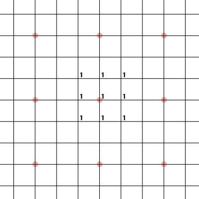
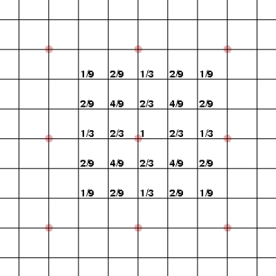
Fig. 10: One grid transfer column stencil associated with the central coarse point using piecewise constants (left) and linear interpolation (right). Only a portion of the mesh is shown and circles denote coarse mesh points.

In these two contexts, the coefficients of $R$, and $P$ do not need to be accessed as they are known ahead of time and have been included in the explicit formulas. In the general situation, the double precision arrays for $R$ and $P$ must be accessed to perform the triple product. In all cases, $A$ is assumed to have a nine point stencil within the interior. Stencils along the boundary have the same structure where entries are dropped if they are associated with points that extend outside of the mesh.

Table 4 illustrates some representative serial timings. The reported mesh sizes refer to the coarse mesh. The corresponding fine mesh is given by $(3n_{x}-2)\times(3n_{y}-2)$ for a coarse $n_{x}\times n_{y}$ mesh. Here, one can see that the structured versions are generally an order of magnitude faster than the unstructured Trilinos/MueLu kernel.

Table 4: Timings (in seconds) for different triple-matrix product kernels. 9 pt Basis (25 pt Basis) indicates $9$ ($25$) point basis functions for $P$ and $R$. Const, Geo, and Generic denote the structured triple product for piecewise constant, ideal geometric, and general grid transfers.

coarse	9 pt Basis		25 pt Basis
mesh size	MueLu	Const	MueLu	Generic	Geo
$140\times 36$	.0024	.0001	.0109	.0012	.0009
$140\times 180$	.0124	.0006	.0572	.0061	.0046
$700\times 180$	.0726	.0070	.2944	.0320	.0240
$700\times 900$	.3702	.0356	1.4786	.1606	.1208

These timings correspond to the core multiply time (excluding a modest amount of time needed in Trilinos to pre/post process data to pre-compute additional information needed for parallel computations). As no inter-region communication is required (due to Theorem 4), the structured serial run times are representative of parallel run times when one region is assigned to each processor. Given the fact the triple product is one of the most costly AMG setup kernels and the fact that the Trilinos matrix-matrix multiply has been optimized many times over the years, these $10x$ gains are significant.

It should be noted, however, that we have not integrated the improved triple products into our framework. In particular, we have not yet developed efficient 3D formulas, which is somewhat labor intensive to perform properly. Additionally, we still have several framework decisions concerning how different structured grid cases are addressed and merged within our generally unstructured AMG package.

6.4 Multigrid for hybrid structured/unstructured meshes

To demonstrate the flexibility of the proposed region MG scheme to handle semi-structured meshes containing unstructured regions we consider a $3\times 3\times 3$ region setup with different regions flagged as either structured or unstructured. The region layout is illustrated in Figure 11 along with a visualization of the aggregates when one region, region $2$, is treated as unstructured. For the numerical tests, we solve a 3D Poisson equation with a $7$-point stencil on a $100\times 100\times 100$ mesh cube using a 3-level W-cycle and piecewise constant interpolation for both the structured multigrid and for the unstructured region AMG. Presently, our implementation only properly addresses a structured/unstructured region combination using piecewise constant interpolation (i.e., the Lemmas presented in this paper are satisfied). Proper extensions for linear interpolation (discussed in Section 5) are planned for a a refactored version of the software. Two iterations of Symmetric Gauss–Seidel are used as the pre and post smoothers, and the coarse grid is solved with a direct solve. The problem is solved to a tolerance of $10^{-6}$. Table 5 shows iteration counts when different regions are marked as unstructured, and the remaining regions are structured.

We see that the introduction of unstructured regions does have a small impact on the convergence rate of the method, with more unstructured regions resulting in slightly more iterations, up to the limit of all regions being treated as unstructured. This is likely a result of suboptimal aggregates being formed along the interfaces due to the forced matching of aggregates between neighboring regions. We have observed that this effect is more pronounced when the coarsening rate in the structured regions differs from the coarsening rate of the unstructured region (in experiments not shown in this paper). Here, the structured regions used a coarsening rate of 3 and the unstructured regions have an approximate coarsening rate of 3 as well.

Table 5: Iteration counts for various structured/unstructured setups. The regions are setup in a $3\times 3\times 3$ format. For structured/unstructured testing, we solve a 3D Laplace equation on a $100\times 100\times 100$ cube. Two iterations of Symmetric Gauss–Seidel are used as the pre smooth and post smooth for a 3-level W-cycle multigrid iteration with piecewise constant interpolation.

Region Layout	Iterations
AMG with no region formatting	17
no unstructured regions	15
no structured regions	18
Front Face unstructured	17
Back Face unstructured	17
Top Face unstructured	17
Bottom Face unstructured	16
Left Face unstructured	17
Right Face unstructured	16
Eight Corners unstructured	16
Region 2 unstructured	15
Region 13 unstructured	16
Region 24 unstructured	15
Regions 2, 13, 24 unstructured	16

Fig. 11: On the left, a visualization of a $3\times 3\times 3$ Region layout on a cube. On the right, an example of the region aggregates, with region 2 unstructured.

7 Concluding remarks

We have presented a generalization of the HHG idea to a semi-structured framework. Within this framework, the original computational domain is decomposed into regions that only overlap at inter-region interfaces. Unknowns along region interfaces are replicated so that each region has its own copy of the solution along its interfaces. This facilitates the use of structured grid kernels within a multigrid algorithm when regions are structured. We have presented a mathematical framework to represent this region decomposition. The framework allows us to precisely define components of a region multigrid algorithm and understand the conditions by which such a region multigrid algorithm is identical to a traditional multigrid algorithm. Using this framework, we illustrate how a region multigrid hierarchy can be constructed without requiring inter-region communication in some cases. We have also presented some ideas towards making the use of such a region multigrid solver less invasive for application developers. These ideas exploit transformations that define conversions between a region representation and a more traditional representation for vectors and matrices. We also illustrated how such a multigrid solver can account for some unstructured regions within the domain. Finally, we have presented some evidence of the potential of such an approach in terms of computational performance.

References

- [1] R. Barret, M. Berry, T. F. Chan, J. Demmel, J. Donato, J. Dongarra, V. Eijkhout, R. Pozo, C. Romine, and H. v. d. Vorst. Templates for the Solution of Linear Systems: Building Blocks for Iterative Methods. SIAM, Philadelphia, PA, USA, 1994.
- [2] B. K. Bergen, T. Gradl, F. Hülsemann, and U. Rüde. A Massively Parallel Multigrid Method for Finite Elements. Computing in Science & Engineering, 8(6):56–62, 2006.
- [3] B. K. Bergen and F. Hülsemann. Hierarchical hybrid grids: data structures and core algorithms for multigrid. Numerical Linear Algebra with Applications, 11(2-3):279–291, 2004.
- [4] B. K. Bergen, G. Wellein, F. Hülsemann, and U. Rüde. Hierarchical hybrid grids: achieving TERAFLOP performance on large scale finite element simulations. International Journal of Parallel, Emergent and Distributed Systems, 22(4):311–329, 2007.
- [5] L. Berger-Vergiat, C. A. Glusa, J. J. Hu, M. Mayr, P. Ohm, A. Prokopenko, C. M. Siefert, R. S. Tuminaro, and T. A. Wiesner. The MueLu Multigrid Framework. https://trilinos.github.io/muelu.html, 2020.
- [6] L. Berger-Vergiat, C. A. Glusa, J. J. Hu, M. Mayr, A. Prokopenko, C. M. Siefert, R. S. Tuminaro, and T. A. Wiesner. MueLu User’s Guide. Technical Report SAND2019-0537, Sandia National Laboratories, Albuquerque, NM (USA) 87185, 2019.
- [7] W. L. Briggs, V. E. Henson, and S. F. McCormick. A Multigrid Tutorial. SIAM, 2nd edition, 2000.
- [8] J. E. Dendy and J. D. Moulton. Black box multigrid with coarsening by a factor of three. Numerical Linear Algebra with Applications, 17(2-3):577–598, 2010.
- [9] A. Dubey, A. Almgren, J. Bell, M. Berzins, S. Brandt, G. Bryan, P. Colella, D. Graves, M. Lijewski, F. Löffler, B. O’Shea, E. Schnetter, B. V. Straalen, and K. Weide. A survey of high level frameworks in block-structured adaptive mesh refinement packages. J. of Par. and Distr. Comput., 74(12):3217 – 3227, 2014.
- [10] R. Falgout, J. Jones, and U. Yang. The design and implementation of hypre, a library of parallel high performance preconditioners. In A. Bruaset and A. Tveito, editors, Numerical Solution of Partial Differential Equations on Parallel Computers, volume 51 of Lecture Notes in Computational Science and Engineering. Springer, Berlin, 2006.
- [11] B. Gmeiner, T. Gradl, F. Gaspar, and U. Rüde. Optimization of the multigrid-convergence rate on semi-structured meshes by local Fourier analysis. Computers & Mathematics with Applications, 65(4):694–711, 2013.
- [12] B. Gmeiner, M. Huber, L. John, U. Rüde, and B. I. Wohlmuth. A quantitative performance study for Stokes solvers at the extreme scale. Journal of Computational Science, 17(3):509–521, 2016.
- [13] B. Gmeiner, M. Mohr, and U. Rüde. Hierarchical Hybrid Grids for Mantle Convection: A First Study. In 2012 11th International Symposium on Parallel and Distributed Computing, pages 309–314, 2012.
- [14] B. Gmeiner, U. Rüde, H. Stengel, C. Waluga, and B. I. Wohlmuth. Performance and Scalability of Hierarchical Hybrid Multigrid Solvers for Stokes Systems. SIAM Journal on Scientific Computing, 37(2):C143–C168, 2015.
- [15] W. Hackbusch. Iterative Solution of Large Sparse Systems of Equations, volume 95 of Applied Mathematical Sciences. Springer, 1994.
- [16] W. Henshaw and D. Schwendeman. Parallel computation of three-dimensional flows using overlapping grids with adaptive mesh refinement. J. of Comp. Phys., 227(16):7469 – 7502, 2008.
- [17] B. Lee, S. Mccormick, B. Philip, and D. Quinlan. Asynchronous fast adaptive composite-grid methods: Numerical results. SIAM J. Sci. Comput., 25:2003, 2003.
- [18] B. Philip and T. Chartier. Adaptive algebraic smoothers. J. of Comp. and Appl. Math., 236(9):2277 – 2297, 2012.
- [19] A. Prokopenko, C. M. Siefert, J. J. Hu, M. Hoemmen, and A. Klinvex. Ifpack2 User’s Guide 1.0. Technical Report SAND2016-5338, Sandia National Laboratories, 2016.
- [20] Y. Saad. Iterative Methods for Sparse Linear Systems. SIAM, Philadelphia, PA, USA, 2003.
- [21] R. Sampath and G. Biros. A parallel geometric multigrid method for finite elements on octree meshes. SIAM J. Sci. Comput., 32(3):1361–1392, 2010.
- [22] J. Schmidt, M. Berzins, J. Thornock, T. Saad, and J. Sutherland. Large scale parallel solution of incompressible flow problems using Uintah and Hypre. In Cluster, Cloud and Grid Computing (CCGrid), 2013 13th IEEE/ACM International Symposium on, pages 458–465, May 2013.
- [23] U. Trottenberg, C. W. Oosterlee, and A. Schuller. Multigrid. Academic Press, 2000.
- [24] P. Vaněk, J. Mandel, and M. Brezina. Algebraic Multigrid By Smoothed Aggregation For Second And Fourth Order Elliptic Problems. Computing, 56:179–196, 1996.