Control Distance IoU and Control Distance IoU Loss Function for Better Bounding Box Regression

Abstract

Numerous improvements for feedback mechanisms have contributed to the great progress in object detection. In this paper, we first present an evaluation-feedback module, which is proposed to consist of evaluation system and feedback mechanism. Then we analyze and summarize the disadvantages and improvements of traditional evaluation-feedback module. Finally, we focus on both the evaluation system and the feedback mechanism, and propose Control Distance IoU and Control Distance IoU loss function (or CDIoU and CDIoU loss for short) without increasing parameters or FLOPs in models, which show different significant enhancements on several classical and emerging models. Some experiments and comparative tests show that coordinated evaluation-feedback module can effectively improve model performance. CDIoU and CDIoU loss have different excellent performances in several models such as Faster R-CNN, YOLOv4, RetinaNet and ATSS. There is a maximum AP improvement of 1.9% and an average AP of 0.8% improvement on MS COCO dataset, compared to traditional evaluation-feedback modules.

1 Introduction

Tremendous works have been made for more accurate and more efficient object detection in recent years. Data augmentation[4, 19, 44], deeper layers of neural networks[9, 25, 35], more complex structured FPN modules[22, 23, 35], and even more number of iterations make the model for object detection state-of-the-art. Undoubtedly these models have achieved remarkable success, however, at the same time these models have huge parameters and unsatisfactory FLOPs, such as Detectron2 Mask R-CNN X101-FPN (parameters: 107M, FLOPs: 277B)[39], ResNet-50 + NAS-FPN (1280@384) (parameters: 104M, FLOPs: 1043B)[10], AmoebaNet+ NAS-FPN +AA(1280) (parameters: 185M, FLOPs: 1317B)[44] and AmoebaNet+ NAS-FPN + AA(1536) (parameters: 209M, FLOPs: 3045B)[44].

This paper focuses the performance improvement of object detection on the evaluation system and feedback mechanism[37] (namely IoU modules and loss functions, combined called evaluation-feedback module) of region proposals without increasing the number of parameters or FLOPs.

The evaluation-feedback modules have 3 main roles: (1) Evaluating region proposals, using ground truth as a criterion. (2) Ranking a set of region proposals (with the same ground truth criterion). (3) Feeding the gap between region proposals (RP) and ground truths (GT) to the neural network, which is used to correct the next evaluation module. Considering evaluation-feedback module is fundamental, this module should be efficient and contain few parameters. A good evaluation-feedback module should meet the following 3 conditions:

• A measure overlapping area.

• The good ability to differentiate and a measure of the degree of difference (sometimes understood as centroid distance and aspect ratio).

• The IoUs calculation can be correlated with loss functions calculation.

Numerous previous studies have tended to focus on the study of feedback mechanism at the expense of evaluation system. In this paper, the Control Distance IoU(CDIoU for short) and the Control Distance IoU loss function (CDIoU loss for short) are proposed and given the same importance. CDIoU has good continuity and derivability, and simplifies the calculation by measuring the distance between RP and GT in a unified way, optimizing the calculation of DIoU and CIoU[42] for centroid distance and aspect ratio, and completing the evaluation quickly. The CDIoU loss function can be correlated with CDIoU calculation, which enables the feedback mechanism to characterize more accurately and feed back the difference between RP and GT, thus making the objective function of the deep learning network converge faster and improving the overall efficiency. The CDIoU and CDIoU loss functions are highly adaptive and show significant improvements on several different models, compared to traditional IoU modules and loss functions. The main contributions of this work can be summarized as:

• The evaluation-feedback module is proposed to consist of evaluation system and feedback mechanism.

• CDIoU is proposed as a new evaluation system and CDIoU loss as a new feedback mechanism.

• Improving the results, while the number of parameters and running time are not increased.

• With wide applicability, make significant improvements on several models.

2 Related Work

The first culmination of deep learning for object detection was the proposal of R-CNN[12], Fast R-CNN[11] and Faster R-CNN[30] models, which laid down the basic framework and data processing for deep learning applied to object detection. YOLO[28] provides a more straightforward way by directly regressing the location of the bounding box and the class to which the bounding exploitation belongs in the output layer, thus transforming the object detection problem into a regression problem. After this, YOLOv2[29], YOLOv3[8], YOLOv4[1] and YOLOv5[18] were proposed, which made the deep learning network not only improve in accuracy but also in computing speed. R-CNN series and YOLO series are the classical representatives of two-stage model[5, 7, 13, 14, 16] and one-stage model[36, 38] in object detection.

Neural network backbone and conv kernel

The backbone networks of deep learning are also evolving. LeNet (1998)[21], AlexNet (2012)[20], VGGNet (2014)[32], GoogLeNet (2014)[33], ResNet (2015)[15], and MobileNet (2017)[17] are preserved in the path of deep learning development. EfficientNet (2019)[34] proposes a more generalized idea on the optimization of current classification networks, arguing that the three common ways of enhancing network metrics, namely widening the network, deepening the network and increasing the resolution, should not be independent of each other.

Along with the backbone, the convolutional kernel[9, 26, 27] is also evolving and changing. Deformable conv[6, 43] adds an offset variable to the position of each sampled point in the convolution kernel, enabling random sampling around the current position without being restricted to the previous regular grid points. Dilated conv[3, 40] can effectively focus on the semantic information of the local pixel blocks, instead of letting each pixel rub together with the surrounding blocks, which affects the detail of segmentation.

Evaluation-feedback module

Based on IoU, GIoU[31] focuses not only on overlapping regions but also on other non-overlapping regions, which can better reflect the overlap of RP and GT. DIoU[42] takes the distance between object and anchor, overlap rate and scale into consideration, which makes the object box regression more stable and does not have problems such as scattering during training like IoU and GIoU.

GIoU loss[40] still has the problems of slow convergence and inaccurate regression. It is found that GIoU first tries to overlap the object box by increasing the size of the detection box, and then uses the IoU loss term to maximize the overlap area with the object box.

DIoU loss and CIoU loss[42] greatly enriched the connotation of IoU calculation results, adding the measurement of difference, including “centroid distance” and “aspect ratio” separately. DIoU loss cannot distinguish which RPs is more similar to GT when the center points of RPs are at the same position. We can know that the calculation process of CIoU loss is more time-consuming, which will eventually drag down the overall training and test time.

3 Analysis of traditional IoUs and loss functions

In object detection, the function of IoUs is to evaluate the similarity between RP and GT. Through the IoU method, the evaluation between RP and GT is given, which plays a fundamental role in the selection of positive and negative samples. In the evaluation-feedback module, the most representative methods are IoU, GIoU, DIoU loss and CIoU loss. They have played a fundamental role in the great progress of object detection, but there still is much room for optimization.

3.1 Analysis of traditional IoUs

IoU is a basic evaluation method, and as shown in Figure 1, the relative position relationship between RP and GT is obviously different. The human brain can clearly distinguish the disadvantages, but the evaluation results of IoU are the same.

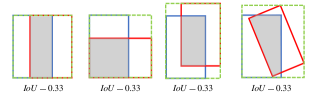
Figure 1: Different relative position relations, the same IoU results

Based on original IoU, many evaluation systems are derived, which enrich the evaluation dimensions of previous IoU from those different aspects.

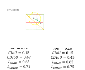
Figure 2: Comparison of IoU GIoU CDIoU and Loss of GIoU & CDIoU

IoU only considers the calculation of overlapping area. Meanwhile, GIoU pays attention to overlapping area and non overlapping area, and strengthens the discussion of evaluation system. However, GIoU obviously ignored the “measurement of difference” between RP and GT.

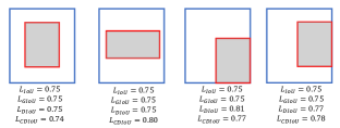
Figure 3: Comparison of multiple IoU losses

The “measurement of difference” between RP and GT include the distance between the center points (centroid) and the ratio of length-width(aspect ratio). DIoU takes centroid into account in the calculation of the evaluation system, but omits aspect ratio. As shown in Figure 2, 3, DIoU can’t recognize the difference between the high-thin region proposal and the short-fat region proposal, and gives them the same value. But in fact, the human brain can easily differentiate which one is better and which position is better.

3.2 IoU:Smooth L1 Loss and IoU Loss

The method of smooth loss is proposed from Fast RCNN[11], which initially solves the problem of characterizing the boundary box loss. Assuming that $x$ is the numerical difference between RP and GT, $L_{1}$ and $L_{2}$ loss are commonly defined as:

$$\mathcal{L}_{1}=|x|\frac{d\mathcal{L}_{2}(x)}{x}=2x,$$ (1)

$$\mathcal{L}_{2}=x^{2}.$$ (2)

The corresponding derivative :

$$\frac{d\mathcal{L}_{1}(x)}{x}=\left\{\begin{array}[]{ll}1&\text{, if }x\geq 0\\ -1&\text{, otherswise ,}\end{array}\right.$$ (3)

$$\frac{d\mathcal{L}_{2}(x)}{x}=2x.$$ (4)

From the derivative of loss function to $x$, we can know that the derivative of loss function $\mathcal{L}_{1}$ to $x$ is constant. In the late training period, when $x$ is very small, if the learning rate is constant, the loss function will fluctuate around the stable value, and it is difficult to converge to higher accuracy. When the derivative of loss function $\mathcal{L}_{2}$ to $x$ is large, its derivative is also very large and unstable at the beginning of training. ${smooth}_{\mathcal{L}_{1}}(x)$ perfectly avoids the shortcomings of $\mathcal{L}_{1}$ and $\mathcal{L}_{2}$ loss.

$$\text{smooth}_{\mathcal{L}_{1}}(x)=\left\{\begin{array}[]{ll}0.5x^{2}&\text{, if }|x|<1\\ |x|-0.5&\text{, otherswise ,}\end{array}\right.$$ (5)

$$\frac{d{smooth}_{\mathcal{L}_{1}(x)}}{x}=\left\{\begin{array}[]{ll}x&\text{, if }|x|<1\\ \pm 1&\text{, otherswise ,}\end{array}\right.$$ (6)

However, in the actual object detection, the loss in box regression task is

$$\mathcal{L}_{loc}\left(t^{u},v\right)=\sum_{i\in\{x,y,w,h\}}\text{smooth}_{\mathcal{L}_{1}}\left(t_{i}^{u}-v_{i}\right),$$ (7)

Where $v=\left(v_{x},v_{y},v_{w},v_{h}\right)$represents the box coordinates of GT, and $t^{u}=\left(t_{x}^{u},t_{y}^{u},t_{w}^{u},t_{h}^{u}\right)$ represents the predicted box coordinates, that is to calculate the loss of four points respectively, and then add them as the bounding box regression loss.

shortcomings:

1.When the above losses are used to calculate the bounding box loss of object detection, the loss of four points is calculated independently, and then the final bounding box loss is obtained by adding. The assumption of this method is that the four points are independent of each other, and there is a certain correlation in fact. The calculation of smooth can not be unified with IoU, which leads to errors of the feedback mechanism and evaluation system.

2.The actual indicator of evaluation is to use IoU, which is not equivalent. IoU loss cannot avoid this scenario,“different RPs, same feedback results” in Figure 2,3.

$$\mathcal{L}_{IoU}=-\ln(IoU),$$ (8)

$$\mathcal{L}_{IoU}=1-IoU.$$ (9)

3.3 GIoU and GIoU Loss

On the premise of not increasing the calculation time, GIoU[31] initially optimized the calculation of IoU for overlapping area, and reduced the calculation error, but GIoU still did not take the measurement of the difference into account in the calculation results.

$$GIoU=IoU-\frac{|C\backslash(A\cup B)|}{|C|},$$ (10)

$$\mathcal{L}_{GIoU}=1-GIoU.$$ (11)

GIoU loss still has the problems of slow convergence and inaccurate regression. It is found that GIoU first tries to overlap the object box (GT) by increasing size of the detection box (RP), and then uses IoU loss term to maximize the overlap area with the object box. At the same time, when the two boxes contain each other, GIoU loss will degenerate into IoU loss. At this time, the alignment of the bounding box becomes more difficult and the convergence is slow.

3.4 DIoU loss and CIoU Loss

DIoU loss and CIoU loss[42] greatly enriched the connotation of IoU calculation results, adding the measurement of difference, including “centroid distance” and “aspect ratio” separately.

$$\mathcal{L}_{DIoU}=1-IoU+\frac{\rho^{2}\left(\mathbf{b},\mathbf{b}^{gt}\right)}{c^{2}}$$ (12)

First of all, DIoU loss cannot distinguish which region proposals are more similar to ground truth when the center points of region proposals are at the same position. Then when two boxes are completely coincident, $\mathcal{L}_{IoU}=\mathcal{L}_{GIoU}=\mathcal{L}_{DIoU}=0$; when two boxes do not intersect, GIoU loss can’t distinguish region proposals exactly and $\mathcal{L}_{GIoU}=\mathcal{L}_{DIoU}\rightarrow 2$.

As shown in the Figure 4, in fact, as long as the center point of the region proposal is on arc $C$ of circle $O$,the penalty terms of DIoU loss are consistent. This is DIoU, which loses the accuracy of the evaluation system.

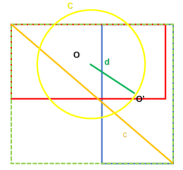
Figure 4: DIoU loss: unuseful relative position relationship between RP and GT

The penalty term of CIoU loss is composed of a factor $\alpha v$ and DIoU loss penalty term, which takes that into account the aspect ratio of RP and GT.

$$\mathcal{L}_{CIoU}=1-IoU+\frac{\rho^{2}\left(\mathbf{b},\mathbf{b}^{gt}\right)}{c^{2}}+\alpha v$$ (13)

The penalty is

$$R_{CIoU}=\frac{\rho^{2}\left(b,b^{gt}\right)}{c^{2}}+\alpha v,$$ (14)

$$\alpha=\frac{v}{(1-IoU)+v},$$ (15)

$$v=\frac{4}{\pi^{2}}\left(\arctan\frac{w^{gt}}{h^{gt}}-\arctan\frac{w}{h}\right)^{2}.$$ (16)

Because the calculation of CIoU loss involves the inverse trigonometric function, and through comparative experiments, we can know that the calculation process of CIoU loss is more time-consuming, which will eventually drag down the overall training time. For detailed comparison tests, see “Ablation studies”.

4 CDIoU and CDIoU loss functions

Based on traditional IoUs and loss functions, CDIoU and CDIoU loss functions are proposed in this paper. Without increasing the operation time, the running efficiency and AP are significantly improved. The CDIoU loss function converges faster and reduces the complexity of the operation significantly.

Control Distance Intersection over Union (CDIoU) is an evaluation method that directly examines the similarity of RP and GT, and it does not directly measure the distance between their centroids and the similarity of their shapes. For detailed information, see Figure 5.

$$\operatorname{diou} =\frac{\|RP-GT\|_{2}}{4\mathrm{MBR}^{\prime}s\text{ diagonal }}$$ (17)

$$=\frac{AE+BF+CG+DH}{4WY}$$

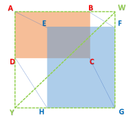
Figure 5: Calculation of CDIoU. Minimum bounding rectangle (MBR) is the smallest rectangle that can contain RP and GT.

$$CDIoU=IoU+\lambda(1-\operatorname{diou})$$ (18)

Although the formula for CDIoU does not mention “centroid distance” and “aspect ratio”, the final calculation results reflect a measure of the degree of difference between RP and GT. The higher the value of CDIoU, the lower the degree of difference; the higher the value of CDIoU, the higher the similarity.

$$\mathcal{L}_{CDIoU}=\mathcal{L}_{IoU_{s}}+\operatorname{diou}$$ (19)

In order to cooperate with the calculation of CDIoU, this paper also proposes the CDIoU loss function. By observing this formula, we can intuitively feel that after backpropagation, the deep learning model tends to pull the four vertices of the region proposal toward the four vertices of the ground truth until they overlap. For detailed information, see Algorithm 1 and Figure 6.

CDIoU and CDIoU loss as a new metric have the following properties: (1) $0\leq\text{ diou }<1$, $\mathcal{L}_{IoU_{s}}$ is the lower limit of $\mathcal{L}_{CDIoU}$. (2) diou broadens the range of $\mathcal{L}_{CDIoU}$. If $\mathcal{L}_{IoU_{s}}=\mathcal{L}_{IoU}$, then $0\leq\mathcal{L}_{CDIoU}<2$, if $\mathcal{L}_{IoU_{s}}=\mathcal{L}_{GIoU}$, then $-1\leq\mathcal{L}_{CDIoU}<2$.

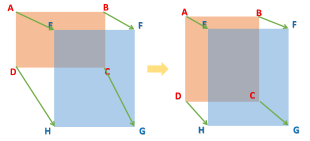
Figure 6: Region proposal turning and variations by CDIoU loss

Algorithm 1 CDIoU and CDIoU loss function

1:RP for region proposal; GT for ground truth;

2:CDIoU and CDIoU loss;

3:For RP and GT, find MBR;

4:compute $IoU=\frac{|RP\cap GT|}{|RP\cup GT|}$ , $\operatorname{diou}=\frac{\|RP-GT\|_{2}}{4\mathrm{MBR}^{\prime}s\text{ diagonal }}$;

5:compute $CDIoU=IoU+\lambda(1-\operatorname{diou})$;

6:compute $\mathcal{L}_{CDIoU}=\mathcal{L}_{IoU_{s}}+\operatorname{diou}$, $\mathcal{L}_{IoU_{s}}$ could be $\mathcal{L}_{IoU}=-\ln(IoU)$, $\mathcal{L}_{IoU}=1-IoU$, $\mathcal{L}_{IoU}=1-IoU$ or $\mathcal{L}_{DIoU}$, $\mathcal{L}_{CIoU}$;

5 Experiments

To ensure the rigidity and richness of the experiments, we did a lot of training and testing on representative models, such as Faster R-CNN, Cascade R-CNN[2], YOLOs and ATSS[41]. Also, we try not to use tricks and allow individual models to compare differences purely due to changes in IoUs or loss functions.

5.1 Working environment and preparation

The following experiments were conducted on MS coco 2017 dataset using two GeForce RTX 2080 Ti GPUs or two Tesla V100 PCIe 32GB GPUs. All models under pytorch or tenserflow framework are standard models without using any tricks.

5.2 CDIoU and CDIoU loss for object detection

In order to verify the effectiveness of CDIoU and CDIoU loss in object detection, experiments are designed and applied to numerous models in this paper. These models encompass existing classical models and emerging models, reflecting certain robustness and wide adaptability. We conduct several experiments to study the robustness of the hyperparameter $\lambda$ in Table 1. Overall, the only hyperparameter $\lambda=0.001$ is quite robust and the proposed CDIoU can be nearly regarded as hyperparameter-free.

$\lambda$	1.0	0.1	0.01	0.001	0.0001
Faster R-CNN	35.6	36.5	37.0	38.5	38.0
ATSS_R_50_FPN	38.1	39.0	39.3	39.5	38.9

Table 1: Analysis(%) of different values of hyperparameter $\lambda$ on the MS COCO val set.

Models	test-dev(%)				val(%)
	AP	APs	APm	APl	AP	APs	APm	APl
Faster R-CNN[11]	36.0	-	-	-	36.0	-	-	-
YOLOv4[1]	41.2	20.4	44.4	56.0	-	-	-	-
RetinaNet-R101 (1024)[24]	40.8	24.1	44.2	51.2	-	-	-	-
ResNet-50 + NAS-FPN (1280@384)[10]	45.4	-	-	-	-	-	-	-
Detectron2 Mask R-CNN R101-FPN[39]	-	-	-	-	44.3	-	-	-
Cascade R-CNN[2]	42.8	23.7	45.5	55.2	-	-	-	-
FCOS[36]	43.2	26.5	46.2	53.3	-	-	-	-
ATSS_R_50_FPN_1x[41]	39.2	-	-	-	39.2	-	-	-
ATSS_dcnv2_R_50_FPN_1x[41]	43.0	-	-	-	43.0	-	-	-
ATSS_R_101_FPN_2x[41]	43.6	-	-	-	43.5	-	-	-
ATSS_dcnv2_R_101_FPN_2x[41]	46.3	-	-	-	46.1	-	-	-
ATSS_X_101_32x8d_FPN_2x[41]	45.1	-	-	-	44.8	-	-	-
ATSS_dcnv2_X_101_32x8d_FPN_2x[41]	47.7	-	-	-	47.7	-	-	-
ATSS_dcnv2_X_101_64x4d_FPN_2x[41]	47.7	-	-	-	47.7	-	-	-
Comparison test 1
ATSS_R_50_FPN_1x + IoU & loss	38.6	20.7	37.4	45.7	38.5	21.0	33.7	50.9
ATSS_dcnv2_R_50_FPN_1x + IoU & loss	41.9	24.0	45.8	53.8	42.5	23.4	44.9	56.9
ATSS_dcnv2_R_101_FPN_2x + IoU & loss	45.8	25.9	48.6	56.9	45.7	28.5	49.7	60.0
ATSS_X_101_32x8d_FPN_2x + IoU & loss	44.5	26.8	47.2	53.2	44.7	27.7	46.1	55.9
ATSS_dcnv2_X_101_32x8d_FPN_2x + IoU & loss	46.8	27.9	49.7	58.7	47.0	29.7	50.1	60.2
ATSS_dcnv2_X_101_32x8d_FPN_2x(MS) + IoU & loss	49.6	31.2	50.5	60.3	49.9	32.7	50.9	61.4
Comparison test 2
Faster R-CNN + CDIoU & loss	38.3	17.3	38.0	54.4	38.5	17.5	37.9	55.7
YOLOv4 + CDIoU & loss	41.4	20.4	46.1	55.8	41.9	21.0	46.7	57.1
RetinaNet-R101 (1024) + CDIoU & loss	41.2	22.5	43.1	50.9	41.5	24.5	45.3	52.7
ResNet-50 + NAS-FPN (1280@384) + CDIoU & loss	45.8	22.1	48.0	65.1	46.0	22.1	48.9	67.4
Detectron2 Mask R-CNN R101-FPN + CDIoU & loss	45.0	21.3	46.0	64.9	45.2	21.9	45.7	66.5
Cascade R-CNN + CDIoU & loss	43.0	25.0	45.7	66.1	43.3	25.3	46.1	67.2
ATSS_R_50_FPN_1x + CDIoU & loss	39.4	22.5	42.2	49.8	39.5	23.0	34.4	52.1
ATSS_dcnv2_R_50_FPN_1x + CDIoU & loss	43.1	24.4	46.0	55.8	43.1	25.4	46.9	57.8
ATSS_dcnv2_R_101_FPN_2x + CDIoU & loss	46.4	27.8	49.7	58.6	46.3	29.3	50.4	61.2
ATSS_X_101_32x8d_FPN_2x + CDIoU & loss	45.2	27.8	48.3	55.2	45.1	28.7	48.5	57.9
ATSS_dcnv2_X_101_32x8d_FPN_2x + CDIoU & loss	47.9	29.6	50.8	60.5	48.1	30.6	51.7	62.7
ATSS_dcnv2_X_101_32x8d_FPN_2x(MS) + CDIoU & loss	50.7	33.2	52.6	62.7	50.9	35.8	53.4	65.3

Table 2: Detection models results with and without IoUs and IoU loss function on the MS COCO val and test-dev set.

• MS means multi-scale testing.

• + CDIoU & loss means that this model uses CDIoU and CDIoU loss as evaluation-feedback module.

• + IoU & loss means that this model uses IoU and IoU loss as evaluation-feedback module.

• The original ATSS models use IoU and GIoU loss as evaluation-feedback module, and the original Faster R-CNN,YOLOv4,RetinaNet-R101,ResNet-50 + NAS-FPN,Detectron2 Mask R-CNN,Cascade R-CNN models use IoU and IoU loss or L1-smooth as evaluation-feedback module.

• FCOS model uses the SSC method, so there is no comparison test.

• Bold fonts indicate the best performance.

• 1x and 2x mean the model is trained for 90K and 180K iterations, respectively.

• All results are obtained with a single model and without any test time data augmentation such as multi-scale, flipping and etc..

• dcnv2 denotes deformable convolutional networks v2.

CDIoU and CDIoU loss are universally adaptable, exhibiting differential performance gains on different models. As shown in Table 2, we can see that the more complex the backbone structure is, the less the CDIoU and CDIoU loss improvement is, while for the basic model, the CDIoU and CDIoU loss improvement is more obvious. By using CDIoU and CDIoU loss, the models in Table 2 improved AP by an average of 0.8%.

5.3 Ablation studies

Faster R-CNN is a classical model, while ATSS is a new model recently. In Table 3, the evaluation system of all models is IoU, the most basic original one. But in the loss function, we selects different calculation functions as feedback mechanism. FPS represents the number of images that can be processed per second. CDIoU loss does not increase the amount of computation and barely improves FPS.

IoUs loss	Model	AP	FPS
L1-smooth	Faster R-CNN[30]	36.0	7.5
IoU loss	Faster R-CNN	36.8	7.7
GIoU loss	Faster R-CNN	36.9	8.5
DIoU loss	Faster R-CNN	38.0	7.9
CIoU loss	Faster R-CNN	38.2	6.3
CDIoU loss	Faster R-CNN	38.5	7.7
L1-smooth	ATSS_R_50_FPN_1x[41]	37.5	11.1
IoU loss	ATSS_R_50_FPN_1x	38.0	10.8
GIoU loss	ATSS_R_50_FPN_1x	39.2	11.0
DIoU loss	ATSS_R_50_FPN_1x	39.0	11.3
CIoU loss	ATSS_R_50_FPN_1x	39.2	8.8
CDIoU loss	ATSS_R_50_FPN_1x	39.4	11.2

Table 3: Comparison of effects and running results(%) of various IoU losses on the MS COCO val set.

• The default evaluation module IoUs is IoU in this table.

As shown in Table 3, we can accurately see that CDIoU loss function can significantly improve the AP results by 0.2$\sim$1.9 $\%$ compared to other loss functions, and this effect is more obvious in traditional and basic models.

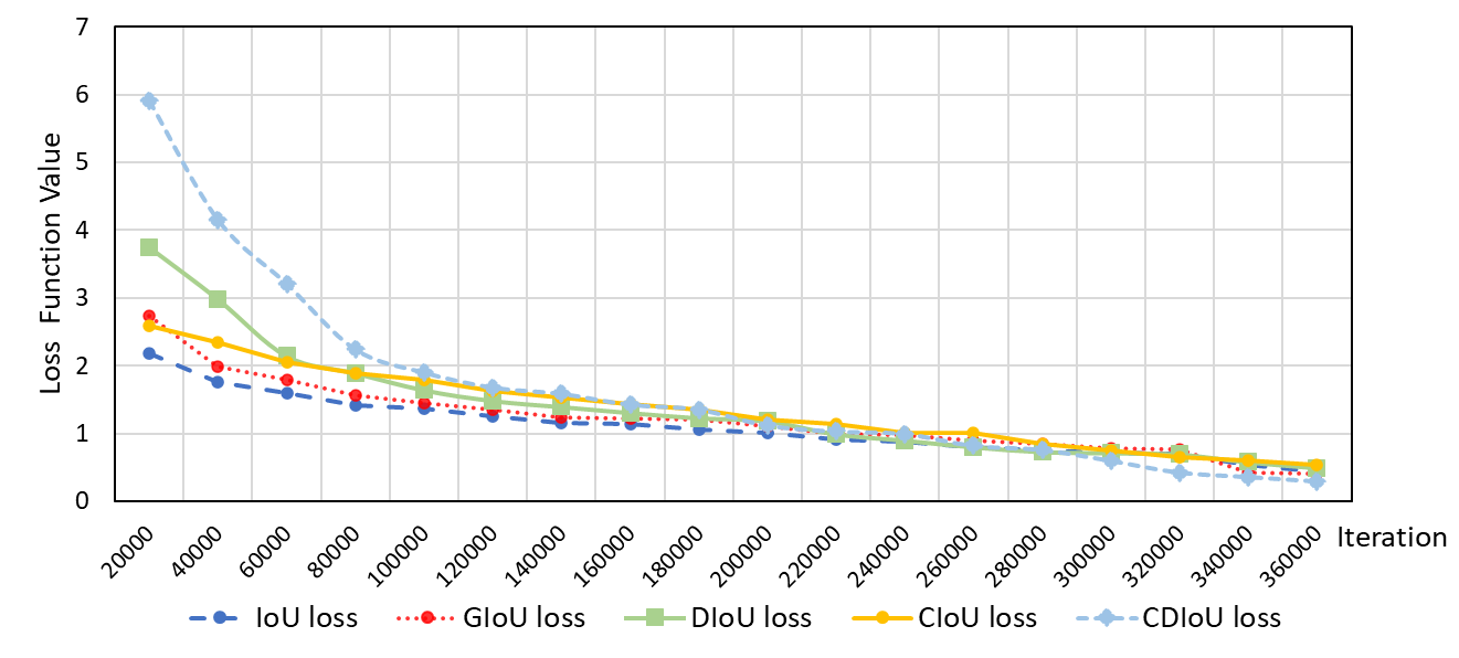
Figure 7: Loss Function value of Faster R-CNN

Figure 8: Loss Function value of ATSS-R-50-FPN-1x

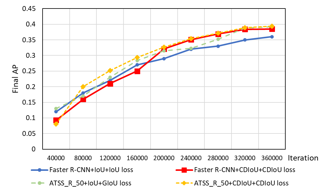
Figure 9: The final AP of Faster R-CNN and ATSS-R-50-FPN-1x

From Figure 7,8 , it is clear that the loss function values of both Faster R-CNN and ATSS-R-50-FPN-1x models drop and reach convergence faster after using CDIoU and CDIoU loss function compared to the other loss functions. The Figure 9 shows that the CDIoU and CDIoU loss functions can help the models achieve higher AP values with fewer iterations. These results show that the CDIoU and CDIoU loss functions have strong convergence and highlight their more accurate evaluation of region proposals.

In order to rigorously verify the effectiveness of CDIoU and CDIoU loss function proposed in this paper, a large number of comparative experiments are designed to suggest supporting evidence. We can learn from Table 4 that CDIoU loss can indeed achieve better results than IoU loss, GIoU loss, DIoU loss, etc., while using the same IoU section.

Model	IoUs		IoU loss functions					AP
	GIoU	CDIoU	IoU loss	GIoU loss	DIoU loss	CIoU loss	CDIoU loss
Faster R-CNN	✓		✓					36.9
Faster R-CNN	✓			✓				37.3
Faster R-CNN	✓				✓			38.0
Faster R-CNN	✓					✓		38.2
Faster R-CNN	✓						✓	38.3
Faster R-CNN		✓	✓					37.1
Faster R-CNN		✓		✓				37.3
Faster R-CNN		✓			✓			38.1
Faster R-CNN		✓				✓		38.3
Faster R-CNN		✓					✓	38.5
ATSS_R_50_FPN_1x	✓		✓					38.0
ATSS_R_50_FPN_1x	✓			✓				39.3
ATSS_R_50_FPN_1x	✓				✓			39.0
ATSS_R_50_FPN_1x	✓					✓		39.2
ATSS_R_50_FPN_1x	✓						✓	39.4
ATSS_R_50_FPN_1x		✓	✓					38.1
ATSS_R_50_FPN_1x		✓		✓				39.3
ATSS_R_50_FPN_1x		✓			✓			39.2
ATSS_R_50_FPN_1x		✓				✓		39.2
ATSS_R_50_FPN_1x		✓					✓	39.5

Table 4: Comparison of effects and running results(%) of various IoUs and IoU loss functions on the MS COCO val set.

• For more information about results of evaluation module IoU, please refer to table 3.

By comparing the above experiments, we can observe that using different IoU modules with different IoU loss functions yields different and thought-provoking results. Combining Table 3,4 , we can analyze that under the same IoU loss function condition, using CDIoU module alone can improve the final result by 0.3 $\sim$ 1.8$\%$; under the same IoU module, using CDIoU loss function alone can improve the final result by 0.2 $\sim$ 1.7$\%$.

At the same time, if IoU module and IoU loss function could be unified in the computational form (eg.GIoU + GIoU loss function and CDIoU + CDIoU loss function), the final result would seem to be better than the sum of the results of using the two optimization schemes independently.

In order to verify the independence and validity of CDIoU and CDIoU loss function, we designs the following comparison test in Table 5, using original IoU + IoU loss(or DIoU loss) function and CDIoU + CDIoU loss function in training and validation stages of the program respectively, and finally comparing their AP results. We use CDIoU and CDIoU loss in the training and validation stages respectively, which can improve the final AP. If we used CDIoU and CDIoU loss in both training and validation stages, we could get more significant improvement results.

5.4 Analysis of experiments

The improvement effect of CDIoU + CDIoU loss tends to decrease as the model is updated. First, as the backbone of the model deepens, the model itself enhances the strength of feature extraction. Second, the continuous improvement of FPN modules also optimizes the function of traditional evaluation systems. The above two points offset the advantages of CDIoU and CDIoU loss compared with the traditional evaluation-feedback modules.

ATSS bridges the gap between anchor-based and anchor-free detection via adaptive training sample selection. Comparison tests on ATSS exclude the essential interference between anchor-based and anchor-free detection. In these tests, the interference of positive and negative sample generation is eliminated, which give tests based on ATSS more representativeness.

Model	Training			validation		AP
	IoU+IoU loss	IoU+GIoU loss	CDIoU+CDIoU loss	Originals	CDIoU+CDIoU loss
Faster R-CNN	✓			✓		36.8
Faster R-CNN	✓				✓	37.2
Faster R-CNN			✓	✓		37.7
Faster R-CNN			✓		✓	38.5
ATSS_R_50_FPN_1x		✓		✓		39.2
ATSS_R_50_FPN_1x		✓			✓	39.3
ATSS_R_50_FPN_1x			✓	✓		39.3
ATSS_R_50_FPN_1x			✓		✓	39.5

Table 5: Comparison of effects and running results(%) in training and validation on the MS COCO train and val set.

• Originals means that original Faster R-CNN uses IoU+IoU loss as evaluation-feedback module and original ATSS_R_50_FPN_1x uses IoU+GIoU loss as evaluation-feedback module.

From Table 5 , we can clearly observe that replacing IoU module and loss function separately can improve the results of the original model, and replacing IoU module and loss function at the same time also has a certain additive effect, achieving the synergy of “one plus one is greater than two”. It lies on the calculation form consistency between evaluation system and feedback mechanism. The numerical fluctuations of the feedback mechanism reflect the differences of the evaluation system, which makes the evaluation-feedback module more targeted.

5.5 Tips to improve performances

In this experiment, we also found some tips to improve AP. These tips are particularly useful for some basic models in this paper.

Floating learning rate

It is a consensus that the learning rate decreases as the iterative process in the experiment. Further, this paper proposes to check the loss every $\mathcal{K}$ iterations and increase the learning rate slightly, if the loss function does not decrease continuously. In this way, the learning rate will decrease and float appropriately at regular intervals to promote the decrease of the loss function.

$$\begin{array}[]{ll}lr=\left\{\begin{aligned} 1.05lr\textit{, Ls}<0\\ lr\textit{, Ls}>0\end{aligned}\right.\\ \textit{Ls}=\operatorname{loss}_{i}-\operatorname{loss}_{i-k}\end{array}$$ (20)

Automatic GT clustering analysis

It is well known that AP can be effectively improved by performing cluster analysis on GT in the original dataset. We adjust anchor sizes and aspect ratios parameters based on the results of this cluster analysis. However, we do not know the number of clusters through the current approach. The main solution is to keep trying the number of clusters $\mathcal{N}$, and then judge by the final result AP. Obviously, this exhaustive method takes a lot of time.

In this paper, automatic GT clustering analysis is proposed, using K-means/PAM, Hierarchical Clustering, Spectral Clustering, DBSCAN and Mean-shift methods respectively, where DBSCAN and Mean-shift methods are able to obtain the number of clusters autonomously. The above methods were evaluated using SSE (sum of the squared errors), Silhouette Coefficient and Calinski-Harabaz, and then two recommended schemes are obtained. These recommended schemes include the number of clusters and the central GT of each cluster. We obtained anchor information from the central GT before executing the complex deep learning network, so that the experiments in this paper are much more efficient.

6 Conclusion

In this paper, we propose that a good evaluation-feedback module should focus on both evaluation system and feedback mechanism. An evaluation-feedback module should meet 3 conditions (overlapping area, the degree of difference and correlated with the loss function) and 3 main roles (evaluation,ranking and feeding the gap). Finally this paper proposes CDIoU and CDIoU loss, a unified interrelated evaluation-feedback module without increasing the model running time and system memory. Through a large number of experiments, we can demonstrate that CDIoU and CDIoU loss can effectively improve the performance of multiple object detection models without increasing parameters or FLOPs in models. By using CDIoU and CDIoU loss, the models improved their AP by an average of 0.8%. And there are a maximum AP performance improvement of 1.9% and an average AP performance of 0.8% improvement on MS COCO dataset, comparing to traditional evaluation-feedback modules. It lies on the calculation form consistency between evaluation system and feedback mechanism, which makes the evaluation-feedback module more targeted.

References

- [1] Alexey Bochkovskiy, Chien-Yao Wang, and Hong-Yuan Mark Liao. Yolov4: Optimal speed and accuracy of object detection. arXiv preprint arXiv:2004.10934, 2020.
- [2] Zhaowei Cai and Nuno Vasconcelos. Cascade r-cnn: Delving into high quality object detection. In Proceedings of the IEEE conference on computer vision and pattern recognition, pages 6154–6162, 2018.
- [3] Liang-Chieh Chen, George Papandreou, Florian Schroff, and Hartwig Adam. Rethinking atrous convolution for semantic image segmentation. arXiv preprint arXiv:1706.05587, 2017.
- [4] Ekin D. Cubuk, Barret Zoph, Dandelion Mane, Vijay Vasudevan, and Quoc V. Le. Autoaugment: Learning augmentation strategies from data. In 2019 IEEE/CVF Conference on Computer Vision and Pattern Recognition (CVPR), 2019.
- [5] Jifeng Dai, Yi Li, Kaiming He, and Jian Sun. R-fcn: Object detection via region-based fully convolutional networks. arXiv preprint arXiv:1605.06409, 2016.
- [6] Jifeng Dai, Haozhi Qi, Yuwen Xiong, Yi Li, Guodong Zhang, Han Hu, and Yichen Wei. Deformable convolutional networks. In Proceedings of the IEEE international conference on computer vision(ICCV), pages 764–773, 2017.
- [7] Kaiwen Duan, Lingxi Xie, Honggang Qi, Song Bai, Qingming Huang, and Qi Tian. Corner proposal network for anchor-free, two-stage object detection. arXiv preprint arXiv:2007.13816(ECCV), 2020.
- [8] Ali Farhadi and Joseph Redmon. Yolov3: An incremental improvement. Computer Vision and Pattern Recognition, cite as, 2018.
- [9] Cheng-Yang Fu, Wei Liu, Ananth Ranga, Ambrish Tyagi, and Alexander C Berg. Dssd: Deconvolutional single shot detector. arXiv preprint arXiv:1701.06659, 2017.
- [10] Golnaz Ghiasi, Tsung Yi Lin, and Quoc V. Le. Nas-fpn: Learning scalable feature pyramid architecture for object detection. In 2019 IEEE/CVF Conference on Computer Vision and Pattern Recognition (CVPR), 2019.
- [11] Ross Girshick. Fast r-cnn. Computer Science(ICCV), 2015.
- [12] Ross Girshick, Jeff Donahue, Trevor Darrell, and Jitendra Malik. Rich feature hierarchies for accurate object detection and semantic segmentation. 2013.
- [13] Kaiming He, Georgia Gkioxari, Piotr Dollár, and Ross Girshick. Mask r-cnn. In Proceedings of the IEEE international conference on computer vision, pages 2961–2969, 2017.
- [14] Kaiming He, Xiangyu Zhang, Shaoqing Ren, and Jian Sun. Spatial pyramid pooling in deep convolutional networks for visual recognition. IEEE transactions on pattern analysis and machine intelligence, 37(9):1904–1916, 2015.
- [15] Kaiming He, Xiangyu Zhang, Shaoqing Ren, and Jian Sun. Deep residual learning for image recognition. In IEEE Conference on Computer Vision & Pattern Recognition, 2016.
- [16] Zhenwei He and Lei Zhang. Multi-adversarial faster-rcnn for unrestricted object detection. In Proceedings of the IEEE International Conference on Computer Vision(ICCV), pages 6668–6677, 2019.
- [17] Andrew G Howard, Menglong Zhu, Bo Chen, Dmitry Kalenichenko, Weijun Wang, Tobias Weyand, Marco Andreetto, and Hartwig Adam. Mobilenets: Efficient convolutional neural networks for mobile vision applications. arXiv preprint arXiv:1704.04861, 2017.
- [18] Glenn Jocher, Alex Stoken, Jirka Borovec, NanoCode012, ChristopherSTAN, Liu Changyu, Laughing, tkianai, yxNONG, Adam Hogan, lorenzomammana, AlexWang1900, Ayush Chaurasia, Laurentiu Diaconu, Marc, wanghaoyang0106, ml5ah, Doug, Durgesh, Francisco Ingham, Frederik, Guilhen, Adrien Colmagro, Hu Ye, Jacobsolawetz, Jake Poznanski, Jiacong Fang, Junghoon Kim, Khiem Doan, and Lijun Yu. ultralytics/yolov5: v4.0 - nn.SiLU() activations, Weights & Biases logging, PyTorch Hub integration, Jan. 2021.
- [19] Mate Kisantal, Zbigniew Wojna, Jakub Murawski, Jacek Naruniec, and Kyunghyun Cho. Augmentation for small object detection. arXiv preprint arXiv:1902.07296, 2019.
- [20] Alex Krizhevsky, Ilya Sutskever, and Geoffrey E Hinton. Imagenet classification with deep convolutional neural networks. Communications of the ACM, 60(6):84–90, 2017.
- [21] Y Lecun and L Bottou. Gradient-based learning applied to document recognition. Proceedings of the IEEE, 86(11):2278–2324, 1998.
- [22] Zuoxin Li and Fuqiang Zhou. Fssd: feature fusion single shot multibox detector. arXiv preprint arXiv:1712.00960, 2017.
- [23] Tsung-Yi Lin, Piotr Dollár, Ross Girshick, Kaiming He, Bharath Hariharan, and Serge Belongie. Feature pyramid networks for object detection. In Proceedings of the IEEE conference on computer vision and pattern recognition, pages 2117–2125, 2017.
- [24] Tsung Yi Lin, Priya Goyal, Ross Girshick, Kaiming He, and Piotr Dollár. Focal loss for dense object detection. In 2017 IEEE International Conference on Computer Vision (ICCV), pages 2999–3007, 2017.
- [25] Wei Liu, Dragomir Anguelov, Dumitru Erhan, Christian Szegedy, Scott Reed, Cheng-Yang Fu, and Alexander C Berg. Ssd: Single shot multibox detector. In European conference on computer vision, pages 21–37. Springer, 2016.
- [26] Hyeonwoo Noh, Seunghoon Hong, and Bohyung Han. Learning deconvolution network for semantic segmentation. In Proceedings of the IEEE international conference on computer vision, pages 1520–1528, 2015.
- [27] Alec Radford, Luke Metz, and Soumith Chintala. Unsupervised representation learning with deep convolutional generative adversarial networks. arXiv preprint arXiv:1511.06434, 2015.
- [28] Joseph Redmon, Santosh Divvala, Ross Girshick, and Ali Farhadi. You only look once: Unified, real-time object detection. In Proceedings of the IEEE conference on computer vision and pattern recognition, pages 779–788, 2016.
- [29] Joseph Redmon and Ali Farhadi. Yolo9000: Better, faster, stronger. In IEEE Conference on Computer Vision & Pattern Recognition, pages 6517–6525, 2017.
- [30] Shaoqing Ren, Kaiming He, Ross Girshick, and Jian Sun. Faster r-cnn: Towards real-time object detection with region proposal networks. IEEE Transactions on Pattern Analysis & Machine Intelligence, 39(6):1137–1149, 2017.
- [31] Hamid Rezatofighi, Nathan Tsoi, Jun Young Gwak, Amir Sadeghian, and Silvio Savarese. Generalized intersection over union: A metric and a loss for bounding box regression. In 2019 IEEE/CVF Conference on Computer Vision and Pattern Recognition (CVPR), 2019.
- [32] Karen Simonyan and Andrew Zisserman. Very deep convolutional networks for large-scale image recognition. arXiv preprint arXiv:1409.1556, 2014.
- [33] Christian Szegedy, Wei Liu, Yangqing Jia, Pierre Sermanet, and Andrew Rabinovich. Going deeper with convolutions. 2014.
- [34] Mingxing Tan and Quoc V Le. Efficientnet: Rethinking model scaling for convolutional neural networks. arXiv preprint arXiv:1905.11946, 2019.
- [35] Mingxing Tan, Ruoming Pang, and Quoc V. Le. Efficientdet: Scalable and efficient object detection. In 2020 IEEE/CVF Conference on Computer Vision and Pattern Recognition (CVPR), 2020.
- [36] Zhi Tian, Chunhua Shen, Hao Chen, and Tong He. Fcos: Fully convolutional one-stage object detection. In 2019 IEEE/CVF International Conference on Computer Vision (ICCV), 2020.
- [37] Yandong Wen, Kaipeng Zhang, Zhifeng Li, and Yu Qiao. A discriminative feature learning approach for deep face recognition. In European conference on computer vision(ECCV), pages 499–515. Springer, 2016.
- [38] Bichen Wu, Forrest Iandola, Peter H Jin, and Kurt Keutzer. Squeezedet: Unified, small, low power fully convolutional neural networks for real-time object detection for autonomous driving. In Proceedings of the IEEE Conference on Computer Vision and Pattern Recognition Workshops, pages 129–137, 2017.
- [39] Yuxin Wu, Alexander Kirillov, Francisco Massa, Wan-Yen Lo, and Ross Girshick. Detectron2. https://github.com/facebookresearch/detectron2, 2019.
- [40] Fisher Yu and Vladlen Koltun. Multi-scale context aggregation by dilated convolutions. 2016.
- [41] Shifeng Zhang, Cheng Chi, Yongqiang Yao, Zhen Lei, and Stan Z. Li. Bridging the gap between anchor-based and anchor-free detection via adaptive training sample selection. In CVPR, 2020.
- [42] Zhaohui Zheng, Ping Wang, Wei Liu, Jinze Li, and Dongwei Ren. Distance-iou loss: Faster and better learning for bounding box regression. In AAAI Conference on Artificial Intelligence, 2020.
- [43] Xizhou Zhu, Han Hu, Stephen Lin, and Jifeng Dai. Deformable convnets v2: More deformable, better results. In 2019 IEEE/CVF Conference on Computer Vision and Pattern Recognition (CVPR), 2019.
- [44] Barret Zoph, Ekin D Cubuk, Golnaz Ghiasi, Tsung-Yi Lin, Jonathon Shlens, and Quoc V Le. Learning data augmentation strategies for object detection. In European Conference on Computer Vision, pages 566–583. Springer, 2020.