Eigenstate thermalization in dual-unitary quantum circuits:
Asymptotics of spectral functions

Abstract

The eigenstate thermalization hypothesis provides to date the most successful description of thermalization in isolated quantum systems by conjecturing statistical properties of matrix elements of typical operators in the (quasi-)energy eigenbasis. Here we study the distribution of matrix elements for a class of operators in dual-unitary quantum circuits in dependence of the frequency associated with the corresponding eigenstates. We provide an exact asymptotic expression for the spectral function, i.e., the second moment of this frequency resolved distribution. The latter is obtained from the decay of dynamical correlations between local operators which can be computed exactly from the elementary building blocks of the dual-unitary circuits. Comparing the asymptotic expression with results obtained by exact diagonalization we find excellent agreement. Small fluctuations at finite system size are explicitly related to dynamical correlations at intermediate times and the deviations from their asymptotical dynamics. Moreover, we confirm the expected Gaussian distribution of the matrix elements by computing higher moments numerically.

I Introduction

Statistical mechanics provides an accurate description of large quantum systems in thermal equilibrium. How isolated quantum systems approach thermal equilibrium, however, has posed major challenges for our understanding of quantum dynamics and statistical physics. In particular, unitarity of time evolution seems to contradict the notion of thermalization from an out-of-equilibrium initial state. This issue was addressed early on by von Neumann Neu1929 , who proposed to study typical or macroscopic physical observables only. Combining this point of view with ideas from random matrix theory lead to the celebrated eigenstate thermalization hypothesis (ETH) which conjectures universal statistical properties of matrix elements of large classes of observables in dependence on the respective energies Deu1991 ; Sre1994 ; Sre1999 . Since then both the validity of ETH and its breakdown as well as the respective implications on thermalization have been investigated in a multitude of studies Rei2015 ; AleKafPolRig2016 ; Deu2018 ; MorIkeKamUed2018 . They are driven by recent experimental realizations of nonequilibrium many-body quantum dynamics GreManHaeBlo2002 ; TroCheFleMcCSchEisBlo2012 ; KinWenWei2006 ; GriKuhLanKitRauSchMazSmiDemSch2012 ; LanErnGeiRauSchKuhRohMazGasSch2015 ; SchHodBorLueFisVosAltSchBlo2015 ; ChoHilZeiSchRubYefKheHusBloGro2016 ; KauTaiLukRisSchPreGre2016 ; NeiRouFanCheKolCheMegBarCam_et_al2016 ; TanKaoLiSeoMalRigGopLev2018 ; BluOmrLevKeeSem_etal2021 .

As we will focus on Floquet systems, which evolve in discrete time, let us formulate ETH explicitly in this context. There ETH conjectures properties of matrix elements $A_{mn}=\bra{m}A\ket{n}$ of an observable $A$ in the quasi-energy eigenbasis $\{\ket{n}:\mathcal{U}\ket{n}=\text{e}^{\text{i}\varphi_{n}}\ket{n}\}$, where $\mathcal{U}$ is the time evolution operator over one period – the so-called Floquet operator. For many-body systems with a clear spatial locality structure, i.e., being defined on a regular lattice with local interactions one typically considers $A$ from a class of a local observables or extensive sums thereof. The ETH ansatz in this setting reads

$$A_{mn}=\langle A\rangle\delta_{mn}+D^{-1/2}f(\omega_{mn})R_{mn}.$$ (1)

Here, $\langle\cdot\rangle$ denotes the thermal average, which in the case of quantum circuits or Floquet systems is taken with respect to the only generally invariant state – the infinite temperature state: $\langle A\rangle=\frac{1}{D}\text{tr}A$, $D=\text{tr}\mathds{1}$. In particular, there is no explicit dependence on the eigenphases, i.e., the quasi-energies $\varphi_{n}$. Without loss of generality the thermal average might be set to zero by subtracting $\langle A\rangle\mathds{1}$ from the operator $A$. Consequently, the nontrivial information is encoded in the second term in which $D$ represents the dimension of the underlying Hilbert space, $R_{mn}$ denote random variables with zero mean and unit variance, and $f(\omega)$ is the spectral function, also called the structure function, of the observable $A$. The latter is a smooth function of the eigenphase differences $\omega_{mn}=\varphi_{n}-\varphi_{m}$. Thus the central questions are: (i) what is the underlying distribution of the random variables $R_{mn}$ or, equivalently, of matrix elements $A_{mn}$, and (ii), what is the functional form of the spectral function $f(\omega)$?

These questions are interrelated and have been investigated in many studies with most of them focusing on the Hamiltonian (continuous-time) case rather than Floquet systems. For instance, the distribution of both diagonal and off-diagonal matrix elements has been confirmed to be generically well described by a Gaussian distribution in the quantum ergodic (or quantum chaotic) regime, whose variance decreases exponentially when increasing the system size BirKolLae2010 ; BreLeBGooRig2020 ; LeBRig2020 ; BeuMoeHaq2015 ; SchJanHeiVid2020:p ; JanStoVidHei2019 ; Noh2021:p ; RicDymSteGem2020 ; BreLeBGooRig2020 ; LeBMalVidRig2019 ; BreGooRig2020 . For these distributions the ratio of the variance of diagonal and off-diagonal matrix elements agrees with random matrix predictions MonRig2017 ; BreLeBGooRig2020 ; LeBRig2020 ; BreGooRig2020 . Deviations from the Gaussian nature of the distribution have been found when the system under consideration approaches the integrable or localized regime Rig2009 ; RoyLevLui2018 ; BreLeBGooRig2020 ; LeBMalVidRig2019 ; BreGooRig2020 as well as for specific nonlocal operators KhaHaqMcC2019 . Moreover, the differences between diagonal matrix elements of neighboring eigenstates as well as the difference between diagonal matrix elements and the corresponding microcanonical expectation value in general vanish with increasing system size RigDunOls2008 ; SanRig2010 ; RigSan2010 ; KimIkeHus2014 ; MonFraSreRig2016 ; BeuMoeHaq2014 ; YosIyoSag2018 ; SteKhoNieGogGem2014 ; MieVid2020 ; SugHamUed2020:p .

More details on the distribution of matrix elements have been obtained by studying the spectral function $f(\omega)$ as it encodes the variance of the distribution of matrix elements NatPor2018b ; JanStoVidHei2019 ; RicDymSteGem2020 ; MonRig2017 ; LeBMalVidRig2019 ; LeBRig2020 and as it sets the energy scale above which nontrivial correlations become relevant Dym2018:p . Generalizations of the spectral function additionally yield higher order correlations of matrix elements ChaDeCha2019 ; FoiKur2019 ; BrePapMitGooSil2021:p . While the small frequency behavior $\omega\to 0$ of the spectral function and the corresponding statistics of diagonal matrix elements $A_{nn}$ encodes equilibrium properties at large times $t\to\infty$, finite frequencies $|\omega|>0$ and the statistics of off-diagonal elements determine fluctuations in equilibrium as well as the dynamics of relaxation to equilibrium. Consequently, the spectral functions governs the decay of dynamical correlations via fluctuation-dissipation relations and linear response theory LuiBar2016 ; RicGemSte2019 ; FoiCugGam2012 ; KhaPupSreRig2014 ; NatPor2019 ; NohSagYeo2020 yielding, e.g., heating rates in driven systems MalRig2019 and sensitive probes to quantum chaos PanClaCamPolSel2020 ; SelPol2020:p .

The aforementioned findings impressively demonstrate the validity of the ETH given by Eq. (1) in generic systems accessible by numerical methods. Exact results, however, are rare due to the complex and analytically intractable dynamics of typical many-body systems. This has triggered the search for exactly solvable chaotic models, from which unitary quantum circuits emerged as a promising candidate. One may hope to derive exact statements on the validity of the ETH as these models allow for analytic results on various other fundamental properties of generic many-body quantum systems. The latter include, e.g., the ballistic spreading of local operators KheVisHus2018 ; RakPolvon2018 ; NahVijHaa2018 ; ChaLucCha2019 ; ChaLucCha2018b ; BerKosPro2019b ; vonRakPolSon2018 ; DiaHaqRibMcC2021:p and the growth of entanglement NahRuhVijHaa2017 ; BerKosPro2019 ; ChaLucCha2018b ; SkiRuhNah2019 ; RakPolKey2019 ; GopLam2019 ; PirBerCirPro2020 ; BerKosPro2020a ; BerKosPro2020b ; KloBerPir2021:p ; BerPir2020 as well as random matrix predictions of spectral correlations ChaLucCha2018a ; ChaLucCha2018b ; KosLjuPro2018 ; BerKosPro2018 ; FriChaDeCha2019 ; FlaBerPro2020 ; KosBerPro2020:p ; BerKosPro2021:p and random state entanglement HamSanZan2012b ; HamSanZan2012a . A particularly fruitful approach assumes an additional duality symmetry between space and time first observed AkiWalGutGuh2016 in a quantum chaotic Ising chain in a pulsed magnetic field Pro2002 . This lead to the notion of dual-unitary quantum circuits BerKosPro2019b in which both propagation in time as well as in space is unitary. Dual-unitarity allows for analytical computations of dynamical correlation functions and spectral correlations as well as the spreading of local operators BerKosPro2018 ; BerKosPro2019 ; BerKosPro2019b ; PirBerCirPro2020 ; BerKosPro2020a ; BerKosPro2020b ; ClaLam2020:p ; BerKosPro2021:p ; KosBerPro2021 ; FlaBerPro2020 ; ReiBer2021:p and provides a manifestation of maximally entangling local evolutions Arul1 ; Arul2 . Morover, the dual space evolution provides deep insights into non-equilibrium properties of general unitary as well as non-unitary Floquet quantum circuits Vedika1 ; Vedika2 ; Dima1 ; Hamazaki ; LuGro2021:p .

Here we aim for analytical answers to the questions on the statistics of matrix elements and the form of the spectral function within the setting of dual-unitary quantum circuits. More precisely, we derive the exact asymptotic form of the spectral function for large system sizes for a class of observables which comprise of sums of local operators. To this end, we analytically compute their autocorrelation functions for times proportional to system size which are fully determined by a completely positive trace preserving (CPTP) map acting on local operators BerKosPro2019b . The latter is constructed using only the elementary building blocks, i.e., the local gates from which the quantum circuit is built. Its spectral properties yield the decay of correlations and asymptotically govern the spectral function. In particular, we find a Lorentzian shape of the spectral function in the presence of isolated slowly decaying modes, while the spectral function becomes almost flat when correlations decay fast.

Using exact diagonalization of dual-unitary qubit circuits we compare the asymptotical result with numerically computed spectral functions and find excellent agreement for generic cases. Nevertheless, we observe finite size deviations which we relate to the dynamics of autocorrelations on intermediate time scales and which are exponentially suppressed when increasing the system size. Going beyond what we can access analytically we additionally extend our numerical studies to higher moments of the frequency resolved empirical distribution of matrix elements. We confirm the latter to be well described by a Gaussian distribution. However, disregarding the frequency dependence we find deviations from a Gaussian distribution. More precisely, we observe exponential tails when the corresponding circuit exhibits slowly decaying modes.

The remainder of this paper is organized as follows. In Sec. II we introduce the quantum circuits studied in our work. Moreover, we review the concept of dual-unitarity and its implications on dynamical correlations of local operators. Subsequently, in Sec. III, we provide details on the computation of the spectral functions and its relation to the dynamics of autocorrelation functions. We also introduce a class of operators for which the latter can be computed exactly. As our main result we derive the asymptotic form of the spectral function for these operators. This is compared with numerical simulations in Sec. IV. We additionally study the distribution of matrix elements there. Eventually, we conclude and summarize our results in Sec. V.

II dual-unitary Quantum Circuits

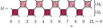
Figure 1: Diagrammatic representation of $\mathcal{U}=\mathcal{U}_{2}\mathcal{U}_{1}$ with $\mathcal{U}_{1}$ and $\mathcal{U}_{2}$ given by Eq. (2) for $2L=10$.

In the following we briefly review dual-unitary quantum circuits and some or their fundamental dynamical properties. In particular we focus on the dynamics of correlation functions of local operators.

II.1 Circuit design

We consider a one-dimensional lattice of qudits subject to a discrete time evolution obtained from a brick-wall circuit design as illustrated in Fig. 1. Each qudit is described by a local Hilbertspace $\mathcal{H}_{x}=\mathbb{C}^{q}$ of dimension $q$ indexed by the sites $x\in\{0,\ldots,2L-1\}$. The latter are arranged on a one-dimensional chain of even length $2L$ with periodic boundary conditions. The system’s total Hilbert space is $\mathcal{H}=\bigotimes_{x=0}^{2L-1}\mathcal{H}_{x}$ and has dimension $\text{dim}\mathcal{H}=D=q^{2L}$. The chain undergoes discrete time evolution governed by the unitary (Floquet) operator $\mathcal{U}$. More precisely, each time step is composed of two half-time steps such that $\mathcal{U}=\mathcal{U}_{2}\mathcal{U}_{1}$ where the half steps are given by

$$\mathcal{U}_{1}=\bigotimes_{x=0}^{L-1}U_{1}\quad\text{and}\quad\mathcal{U}_{2}=\mathcal{T}\left(\bigotimes_{x=0}^{L-1}U_{2}\right)\mathcal{T}^{-1},$$ (2)

see Fig. 1 for a diagrammatic representation of the resulting time evolution operator $\mathcal{U}$. Here, $U_{1},U_{2}\in\text{U}(q^{2})$ describe the interaction of qudits on even sites with their right and left nearest neighbor, respectively. In order to avoid undesired symmetries we choose $U_{1}\neq U_{2}$. Moreover, $\mathcal{T}$ denotes a periodic shift on the lattice defined in the canonical basis by $\mathcal{T}\left(\ket{i_{0}}\otimes\ket{i_{1}}\otimes\ldots\otimes\ket{i_{2L-1}}\right)=\ket{i_{2L-1}}\otimes\ket{i_{0}}\otimes\ldots\otimes\ket{i_{2L-2}}$, where $\{\ket{i},i=0,\ldots,q-1\}$ is an orthonormal basis of $\mathcal{H}_{x}$. By construction, $\left[\mathcal{T}^{2},\mathcal{U}\right]=0$ and consequently both $\mathcal{U}$ and $\mathcal{T}^{2}$ can be diagonalized simultaneously yielding common eigenstates $\ket{n}$ and their respective eigenphases, i.e.,

$$\mathcal{U}\ket{n}=\text{e}^{\text{i}\varphi_{n}}\ket{n}\quad\text{and}\quad\mathcal{T}^{2}\ket{n}=\text{e}^{\text{i}\frac{2\pi k_{n}}{L}}\ket{n},$$ (3)

with (quasi-) momenta $k_{n}\in\{0,\ldots,L-1\}$ as $\mathcal{T}^{2L}=\mathds{1}_{\mathcal{H}}$.

Despite their simple structure quantum circuits similar to those described above are tractable by exact analytical methods only in certain limiting cases. Here, we require that the local gates $U_{1}$ and $U_{2}$ satisfy a property dubbed dual-unitarity in order to allow for analytic calculations. To this end, for a given local two-qudit gate $U$ we assign the dual gate $\tilde{U}$ defined by a reshuffling of matrix entries as BerKosPro2019b

$$\bra{i_{1}}\otimes\bra{j_{1}}\tilde{U}\ket{i_{2}}\otimes\ket{j_{2}}:=\bra{j_{2}}\otimes\bra{j_{1}}U\ket{i_{2}}\otimes\ket{i_{1}}.$$ (4)

The original gate $U$ is then called dual-unitary, if its dual $\tilde{U}$ is unitary as well, i.e. $\tilde{U}\in U(q^{2})$. Note that for a generic local gate its dual is in general not unitary. In what follows we assume both local gates $U_{1}$ and $U_{2}$ to be dual-unitary. While the local gates $U_{i}$ are the elementary building blocks of the time evolution operator $\mathcal{U}$ their duals can be thought of as the elementary building blocks of a spatial transfer matrix describing propagation in space rather then time. Dual-unitarity implies that propagation in space is unitary as well and thus gives rise to a structural symmetry between space and time.

Whereas the complete characterization or classification of the set of dual-unitary gates is an open problem for general $q$, it has been solved for $q=2$ in Ref. BerKosPro2019b . There it has been shown that the dual-unitarity condition fixes only $2$ out of $16$ parameters specifying an arbitrary unitary two-qubit gate $U\in U(4)$. Hence dual-unitarity is not as restricting as one might think naively.

II.2 Dynamical correlations of local operators

The symmetry between space and time due to dual-unitarity imposes strong restrictions on the form of dynamical correlations [see definition (6) below] of local operators. Intuitively, the brickwork pattern and the unitarity of propagation in time restricts nonzero correlations between local operators to a light cone in space while the unitarity of propagation in space restricts nonzero correlations to a light cone in time. Consequently, correlations can be non-vanishing only on the intersection of both light cones, namely on light-rays of the form $y=x\pm 2t$. This intuitive picture has been made rigorous in Ref. BerKosPro2019b and has been found to be structurally stable upon generic, non-dual-unitary perturbations KosBerPro2021 , i.e., the dual-unitary contribution dominates dynamical correlations even under small perturbations. We briefly review the results obtained in Ref. BerKosPro2019b in what follows.

Consider a Hermitian and traceless operator $a\in\text{End}(\mathbb{C}^{q})$ and its embedding into $\text{End}(\mathcal{H})$ for a fixed lattice site $x\in\{0,\ldots,2L-1\}$ given by

$$a_{x}=\left(\bigotimes_{y=0}^{x-1}\mathds{1}_{\mathcal{H}_{y}}\right)\otimes a\otimes\left(\bigotimes_{y=x+1}^{2L-1}\mathds{1}_{\mathcal{H}_{y}}\right).$$ (5)

That is, $a_{x}$ acts nontrivially only at lattice site $x$. Note that being traceless ensures that $a$ and $a_{x}$ are Hilbert-Schmidt orthogonal to the respective identities $\mathds{1}_{\mathbb{C}^{q}}$ and $\mathds{1}_{\mathcal{H}}$. We will always assume $a$ to be Hilberg-Schmidt normalized, i.e., $\text{tr}(a^{2})=q$ and thus $\text{tr}(a_{x}^{2})=q^{2L}$ for all $x$. We are interested in dynamical correlation functions $C_{ab}(x,y,t)=\langle a_{x}(t)b_{y}\rangle$ between such local operators $a_{x}$ and $b_{y}$, where $a_{x}(t)=\mathcal{U}^{-t}a_{x}\mathcal{U}^{t}$ is the time evolved operator in the Heisenberg picture. The average is taken with respect to the infinite temperature state, $\langle\,\cdot\,\rangle=q^{-2L}\text{tr}(\,\cdot\,)$, which constitutes the natural thermodynamic steady state for the quantum circuits under consideration. Thus the dynamical correlations are given by

$$C_{ab}(x,y,t)=q^{-2L}\text{tr}\left(\mathcal{U}^{-t}a_{x}\mathcal{U}^{t}b_{y}\right).$$ (6)

For times $t\leq\lfloor L/2\rfloor$ the intuitive picture sketched above applies. More precisely a trivial extension of the results obtained in Ref. BerKosPro2019b to the present case of different local gates $U_{1}$ and $U_{2}$ in each half time step yields

$$C_{ab}(x,y,t)=\delta_{(x+2\nu t-y)\,(\text{mod }2L)}\frac{1}{q}\text{tr}\left(\mathcal{M}_{\nu}^{t}(a)b\right).$$ (7)

The first factor is a Kronecker delta which is one if $y=x+2\nu t\,(\text{mod }2L)$ and zero otherwise, where $\nu=-1$ if $x$ is even and $\nu=1$ if $x$ is odd. Thus it restricts nonzero correlations to light rays $y=x+2\nu t\,(\text{mod }2L)$ for initial times $t\leq\lfloor L/2\rfloor$. Due to our choice of periodic boundary conditions this statement applies to all lattice sites $x$ and we do not have to take scattering effects at open boundaries into account, which would spoil Eq. (7) for $x$ close to the boundary. In the second factor of the right hand side of Eq. (7) the trace is taken in $\text{End}(\mathbb{C}^{q})$ and $\mathcal{M}_{\nu}$ is a CPTP map $\text{End}(\mathbb{C}^{q})\to\text{End}(\mathbb{C}^{q})$. Similar to the structure of the whole circuit $\mathcal{M}_{\nu}$ factors into two half time steps as $\mathcal{M}_{\nu}=\mathcal{M}_{\nu,2}\mathcal{M}_{\nu,1}$ with

$$\mathcal{M}_{+,i}(a) =\frac{1}{q}\text{tr}_{1}\left[U_{i}^{-1}\left(a\otimes\mathds{1}_{\mathbb{C}^{q}}\right)U_{i}\right],$$ (8)

$$\mathcal{M}_{-,i}(a) =\frac{1}{q}\text{tr}_{2}\left[U_{i}^{-1}\left(\mathds{1}_{\mathbb{C}^{q}}\otimes a\right)U_{i}\right],$$ (9)

where the partial trace is taken over the first or second tensor factor of $\mathbb{C}^{q}\otimes\mathbb{C}^{q}$ respectively.

As a consequence the dynamics of correlation functions between local operators is determined by the properties of the maps $\mathcal{M}_{\nu}$ in the thermodynamic limit $L\to\infty$. More precisely, the decay of such correlations is encoded in the spectrum of $\mathcal{M}_{\nu}$, which is contained within the complex unit disk. The spectral properties thus allow for a classification of dual-unitary circuits by their ergodic properties. In any case $\mathcal{M}_{\nu}$ has the trivial eigenvalue $1$ with eigenvector (eigenoperator) $\mathds{1}_{\mathbb{C}^{q}}$, meaning that the maps $\mathcal{M}_{\nu}$ are also unital. Moreover, the real subspace of traceless Hermitian operators of $\text{End}(\mathbb{C}^{q})$ is invariant under $\mathcal{M}_{\nu}$. Here, we consider the case where $\mathcal{M}_{\nu}$ is strictly contracting on this subspace, i.e., it has no other eigenvalue of modulus one other than the trivial one. This class of dual-unitary circuits is called ergodic and mixing as in the thermodynamic limit all dynamical correlations $C_{ab}(x,y,t)$ tend to zero as $\lambda_{\nu}^{t}$ for $t\to\infty$, where $\lambda_{\nu}$ is the largest (in modulus) nontrivial eigenvalue of $\mathcal{M}_{\nu}$ BerKosPro2019b . Additionally, ergodic and mixing dual-unitary circuits exhibit quantum chaos in the spectral sense as their spectral form factor exactly follows random matrix predictions BerKosPro2021:p . They moreover generate linear growth of operator entanglement and hence of the complexity of local operators upon time evolution BerKosPro2020a .

III Spectral function for sums of local observables

Having introduced the models under consideration we proceed by commenting on the spectral function $f(\omega)$ which appears in the formulation of ETH in Eq. (1). To this end, consider a Hermitian and traceless operator $A\in\text{End}(\mathcal{H})$. We briefly discuss how the spectral function corresponding to $A$ emerges from statistical properties of its matrix elements as well as from its dynamical autocorrelation function. For the latter we derive our main result in the form of an asymptotic large $L$ expression for the spectral function for a class operators, which consists of spatial sums of the local operators discussed in the previous section.

III.1 Spectral function from the distribution of matrix elements

In the following we describe the spectral function as the second moment of the frequency resolved distribution of matrix elements of $A$ in the basis of eigenstates of $\mathcal{U}$. We study the statistics of matrix elements $A_{mn}$ for which $\omega_{mn}$ is sufficiently close to a given frequency $\omega\in\left[-\pi,\pi\right)$. More precisely, we fix $0<\Delta\ll 1$ and consider only matrix elements for which $\omega_{mn}\in I_{\Delta}(\omega):=\left[\omega-\Delta/2,\omega+\Delta/2\right)$. The second moment, i.e., the variance of their distribution is given by

$$\text{var}_{\omega}(A_{mn})=\frac{1}{N(\omega)}\sum_{m,n=0}^{q^{2L}-1}|A_{mn}|^{2}1_{I_{\Delta}(\omega)}(\omega_{mn})$$ (10)

where $1_{I_{\Delta}(\omega)}$ denotes the characteristic function of $I_{\Delta}(\omega)$. The normalization $N(\omega)$ is determined by the number of frequencies $\omega_{mn}$ in $I_{\Delta}(\omega)$, i.e.,

$$N(\omega)=\sum_{m,n=0}^{q^{2L}-1}1_{I_{\Delta}(\omega)}(\omega_{mn}).$$ (11)

Asymptotically one has $N(\omega)=q^{4L}\Delta/(2\pi)$ as in chaotic systems the eigenphases and consequently also the frequencies are uniformly distributed in $\left(-\pi,\pi\right]$. Note that at $\omega=0$ the $q^{2L}$ real diagonal matrix elements contribute systematically to $N(0)$. We neglect this issue as on the one hand we restrict most of our discussion to nonzero frequencies, and on the other hand, for $\Delta\gg 2\pi q^{-2L}$ the statistics of matrix elements is not significantly affected by the diagonal matrix elements.

For operators $A$ compatible with the two-site shift invariance of $\mathcal{U}$, i.e. $\left[A,\mathcal{T}^{2}\right]=0$, matrix elements between eigenstates of different momentum vanish. Therefore, we may consider the distribution of matrix elements of the operator $\mathcal{P}_{k}A\mathcal{P}_{k}$ in the basis of eigenvectors of $\mathcal{P}_{k}\mathcal{U}\mathcal{P}_{k}$ corresponding to nonzero eigenvalues, where $\mathcal{P}_{k}$ denotes the orthogonal projection onto the eigenspace of $\mathcal{T}^{2}$ corresponding to momentum $k$. We denote the frequency resolved second moment of this distribution by $\text{var}_{\omega}^{(k)}\!\left(A_{mn}\right)$, for which the normalization asymptotically reads $N_{k}(\omega)=q^{4L}\Delta/(2\pi L^{2})$ PinPro2007 , and obtain the variance of the full distribution by

$$\text{var}_{\omega}(A_{mn})=\frac{1}{L^{2}}\sum_{k=0}^{L-1}\text{var}_{\omega}^{(k)}\left(A_{mn}\right),$$ (12)

see App. A for a derivation.

Independent from the symmetries of $A$, the spectral function can be related to the variance of matrix elements $A_{mn}$ by replacing the latter with the ETH ansatz (1) in Eq. (10). Using the smoothness of $f(\omega)$ as well as the assumption that $R_{mn}$ has unit variance this yields

$$|f(\omega)|^{2}=q^{2L}\text{var}_{\omega}(A_{mn}).$$ (13)

Thus, the spectral function is determined by the variance of the frequency resolved distribution of matrix elements.

III.2 Spectral function from autocorrelation functions

On the other hand, the spectral function may be extracted from the autocorrelation function $\langle A(t)A\rangle$ of the operator $A$. Representing $\mathcal{U}^{\pm t}$ by its respective spectral decomposition yields

$$g(t):=\langle A(t)A\rangle=q^{-2L}\sum_{m,n=0}^{q^{2L}-1}|A_{mn}|^{2}\text{e}^{\text{i}\omega_{mn}t}$$ (14)

for the autocorrelation function. Note that due to the cyclicity of the trace-like infinite temperature state one has $g(t)=g(-t)$. Fourier transforming $g(t)$ as $\hat{g}(\omega)=\sum_{t}g(t)\text{e}^{\text{i}\omega t}$ gives

$$\hat{g}(\omega)=2\pi q^{-2L}\sum_{m,n=0}^{q^{2L}-1}|A_{mn}|^{2}\delta(\omega-\omega_{mn}).$$ (15)

This singular expression is regularized by integrating over $I_{\Delta}(\omega)$ giving the second moment (10) which in combination with Eq. (13) leads to

$$|f(\omega)|^{2}=\frac{q^{4L}}{2\pi N(\omega)}\int_{I_{\Delta}(\omega)}\hat{g}(\tilde{\omega})\text{d}\tilde{\omega}.$$ (16)

Often evaluating the integral is omitted by considering autocorrelations only up to some finite cut-off time $T$. This effectively broadens the $\delta$ distributions as they are replaced by a strongly peaked smooth function of effective width $\sim 1/T$. We denote the resulting finite time Fourier transform by $\hat{g}_{T}(\omega)=\sum_{t=-T}^{T}g(t)\text{e}^{\text{i}\omega t}$. Choosing $\Delta$ sufficiently small compared to the scale on which $\hat{g}_{T}(\omega)$ varies we may replace the integral in Eq. (16) by $\Delta\hat{g}_{T}(\omega)$ yielding

$$|f(\omega)|^{2}=\hat{g}_{T}(\omega).$$ (17)

Thus the spectral function is just a regularized Fourier transform of an autocorrelation function of $A$.

III.3 Asymptotical spectral functions

Our objective in the following is to identify a class of operators for which $\hat{g}_{T}(\omega)$ can be calculated exactly for sufficiently large cut-off times $T$. The local Hermitian traceless operators $a_{x}$ discussed in Sec. II seem as a natural candidate but dual-unitarity causes their autocorrelation functions to vanish exactly for $t<L$. This may be overcome by considering sums of such operators acting on different lattice sites instead. The simplest and most convenient examples of such operators are sums

$$A=\frac{1}{\sqrt{L}}\sum_{x=0}^{L-1}a_{2x+\mu},$$ (18)

which act nontrivially on the even ($\mu=0$) or on the odd ($\mu=1$) sublattice only. Moreover, $A$ is normalized as $\langle A^{2}\rangle=1$. This normalization ensures that the following results do not depend on the system size $L$.

The autocorrelation function for $A$ can be decomposed into correlation functions of the local operators $a_{2x+\mu}$ as

$$\langle A(t)A\rangle=\frac{1}{L}\sum_{x,y=0}^{L-1}C_{aa}(2x+\mu,2y+\mu,t)$$ (19)

For times $t\leq\lfloor L/2\rfloor$ the individual contributions $C_{aa}(2x+\mu,2y+\mu,t)$ are given by Eq. (7) and thus are nonzero only if $y=x+\nu t\,(\text{mod }L)$, where $\nu=2\mu-1$. More precisely, we find

$$\langle A(t)A\rangle =\frac{1}{L}\sum_{x=0}^{L-1}C_{aa}(2x+\mu,(2x+\mu+2\nu t)\,(\text{mod }2L),t)$$

$$=\frac{1}{q}\text{tr}\left(\mathcal{M}_{\nu}^{t}(a)a\right)$$ (20)

independent of the system size $L$. Therefore we choose $T=\lfloor L/2\rfloor$ as the cut-off time and obtain

$$\hat{g}_{\lfloor L/2\rfloor}(\omega;a)=1+\frac{2}{q}\sum_{t=1}^{\lfloor L/2\rfloor}\cos(\omega t)\,\text{tr}\left(\mathcal{M}_{\nu}^{t}(a)a\right),$$ (21)

where we explicitly include the dependence on $a$ in the notation. As the expression (20) decays exponentially at least as $\lambda_{\nu}^{t}$ for $t\to\infty$, with $\lambda_{\nu}$ the largest modulus eigenvalue of $\mathcal{M}_{\nu}$, its Fourier transform is well behaved for $L\to\infty$ and thus Eq. (21) gives rise to a smooth function. This determines the large $L$ asymptotics of the spectral function

$$|f_{\infty}(\omega;a)|^{2}=1+\frac{2}{q}\sum_{t=1}^{\infty}\cos(\omega t)\,\text{tr}\left(\mathcal{M}_{\nu}^{t}(a)a\right)$$ (22)

and constitutes our first main result. As it is obtained for times up to $T=\lfloor L/2\rfloor$ one can expect this to yield the spectral function for frequencies $|\omega|\gtrsim\pi/L$ in finite systems and thus for all nonzero frequencies in the thermodynamic limit $L\to\infty$. Deviations of $f(\omega;a)$ around $f_{\infty}(\omega;a)$ are due to the correlations deviating from Eq. (20) for times $t>\lfloor L/2\rfloor$. More precisely, for thermalizing systems the autocorrelation function equilibrates to a value exponentially small in system size, determined by the diagonal matrix elements corresponding to $\omega=0$, and exhibits residual fluctuations only. These times, however, do not contribute to the spectral function due to the smoothing within the finite frequency window $I_{\Delta}(\omega)$ of width $\Delta$ present in Eqs. (10) and (16), respectively. In contrast, deviations from the asymptotic spectral function at finite system size may be due to the the dynamics of autocorrelation functions at intermediate time scales. We postpone the discussion thereof to the next section when considering a concrete example.

A detailed analysis of $|f_{\infty}(\omega;a)|^{2}$ is possible for a suitable choice of the operator $a$. To this end let $a=a_{\lambda}$ be a Hermitian eigenvector of $\mathcal{M}_{\nu}$ corresponding to a real eigenvalue $\lambda$. We may write $|\lambda_{\nu}|=\text{e}^{-\gamma}$ with $\gamma>0$. The latter is the rate with which the autocorrelation Eq. (20) decays, i.e., $\langle A(t)A\rangle=\lambda^{t}\propto\text{e}^{-\gamma t}$. This allows for evaluating its Fourier transform exactly, see App. B, yielding

$$|f_{\infty}(\omega;a_{\lambda})|^{2}=\frac{\sinh(\gamma)}{\cosh(\gamma)-\text{sign}(\lambda)\cos(\omega)}.$$ (23)

For fast decaying modes, i.e., large $\gamma$ the spectral function (23) is essentially flat, $|f_{\infty}(\omega;a_{\lambda})|^{2}\approx 1$. In contrast, for slowly decaying modes, i.e., $\gamma\ll 1$ the spectral function is strongly peaked around $\omega=0$ ($\lambda>0$) or $\omega=\pi$ ($\lambda<0$). Indeed, by expanding both numerator and denominator up to second order in $\gamma$ around $0$ and $\omega$ around the peak yields a Lorentzian spectral function with full width at half maximum given by $2\gamma$ and peak height $2/\gamma$; see Fig. 2(a) for some examples of the shape of $|f_{\infty}(\omega;a_{\lambda})|^{2}$. Note, that the (leading) eigenvalues of $\mathcal{M}_{\nu}$ are not necessarily real, but may come in complex conjugate pairs $\lambda,\bar{\lambda}\in\mathbb{C}$, for which the corresponding eigenvectors are not Hermitian but come in Hermitian conjugate pairs. Moreover, the linear map $\mathcal{M}_{\nu}$ is in general not diagonalizable leading to possibly nontrivial Jordan blocks (in case of degenerate eigenvalues) and thus to polynomial corrections to the pure exponential decay of correlations when considering generalized eigenvectors.

IV Numerical tests

In this section we compare the asymptotic expressions, Eqs. (22) and (23), with spectral functions obtained from exact diagonalization of representative example systems, for which we find excellent agreement in generic cases. Additionally, we study the frequency resolved distribution of matrix elements numerically in more detail. In particular, we confirm that the latter coincides with a complex Gaussian distribution for frequencies $|\omega|>\pi/L$ by computing higher moments of the distribution.

For our numerical simulation we consider chains of qubits, i.e., $q=2$ for which an exhaustive parameterization of dual-unitary gates $U\in\text{U}(4)$ is given by BerKosPro2019b (SM)

$$U=\left(u_{+}\otimes u_{-}\right)V(J)\left(v_{-}\otimes v_{+}\right).$$ (24)

Here, $u_{\pm},v_{\pm}\in\text{U}(2)$ and

$$V(J)=\exp\left(-\text{i}\left[\frac{\pi}{4}\sigma^{x}\otimes\sigma^{x}+\frac{\pi}{4}\sigma^{y}\otimes\sigma^{y}+J\sigma^{z}\otimes\sigma^{z}\right]\right)$$ (25)

with $J\in\left(\pi/4,\pi/4\right]$ and Pauli matrices $\sigma^{x}$, $\sigma^{y}$, and $\sigma^{z}$. In the following we set $J=0$ in both $U_{1}$ and $U_{2}$ rendering the resulting circuits ergodic and mixing BerKosPro2019b (SM). Moreover, for the corresponding local $\text{U}(2)$ matrices, denoted by $u_{\pm,i},v_{\pm,i}$ for both half time steps we choose generic examples reported in Appendix C. We consider the operator $a=\sigma^{z}\in\text{End}(\mathbb{C}^{2})$ in order to construct $A$ via Eq. (18) on the odd sublattice ($\mu=\nu=+1$). We fix the lattice size as $2L=16$ in what follows.

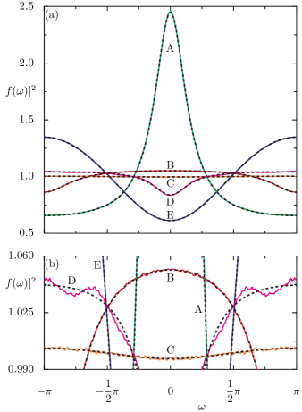
Figure 2: Spectral function of the operator $A$, Eq.(18) for five representative realizations of the dual-unitary circuit $\mathcal{U}$ with $2L=16$ labeled by A-E. The corresponding asymptotic expressions (26) are depicted as dashed black lines. The lower panel (b) is a magnification of panel (a).

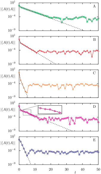
Figure 3: Autocorrelation functions of the operator $A$ versus time for systems A-E with $2L=16$ on a semilogarithmic scale (colored symbols connected by lines). The asymptotic autocorrelation functions $\alpha\lambda_{\nu}^{t}$ ($t\geq 1$) are depicted as black dashed lines.

IV.1 Spectral function

For the quantum circuits introduced above we compute the spectral function of $A$ as described in Sec. III.1 utilizing the two-site shift invariance of $A$, i.e., $\left[\mathcal{T}^{2},A\right]=0$. We first construct the projectors $\mathcal{P}_{k}$ onto the subspaces of momentum $k$ and subsequently diagonalize $\mathcal{U}$ in each subspace. This allows for computing the variance $\text{var}_{\omega}^{(k)}(A_{mn})$ for each momentum $k$. To this end we subdivide the interval $\left[-\pi,\pi\right)$ into $N_{\Delta}=201$ subintervals $I_{\Delta}(\omega_{i})$ of width $\Delta=2\pi/N_{\Delta}$ with centers $\omega_{i}=2\pi(i+1/2)/N_{\Delta}-\pi$ for $i\in\{0,\ldots,N_{\Delta}-1\}$. Having determined $\text{var}_{\omega}^{(k)}(A_{mn})$ we obtain $\text{var}_{\omega}(A_{mn})$ from Eq. (12). Eventually this yields the spectral function via Eq. (13). We obtain the spectral function by this procedure for five different realizations of the circuit labeled by A-E as depicted in Fig. 2 by thin (colored) lines. The spectral functions vary between being almost flat (System C) and being sharply peaked (System A) therefore covering the typical behavior predicted by Eq. (23). Figure 2(b) depicts a magnification around $|f(\omega)|=1$.

As $a=\sigma^{z}$ is not an eigenvector of $\mathcal{M}_{\nu}$ in general the description presented in Sec. III.3 does not apply directly. Nevertheless, the latter can be adapted to the qubit circuits at hand, which we illustrate in the following. We start by noting that in the present case $\mathcal{M}_{\nu}$ can generically be diagonalized and for $J=0$ exhibits two eigenvalues equal to $0$ and only one nontrivial and nonzero eigenvalue $\lambda$, which is necessarily real. We report these eigenvalues for both $\mathcal{M}_{+}$ and $\mathcal{M}_{-}$ in Table 1 for the systems under consideration. We denote the corresponding hermitian eigenvector by $a_{\lambda}$. As $\mathcal{M}_{\nu}$ can be diagonalized we can expand $a$ in the basis consisting of its nonorthogonal eigenvectors. To this end let $\bar{a}_{\lambda}$ denote the hermitian and traceless left eigenvector corresponding to $\lambda$. That is $\bar{a}_{\lambda}$ is an eigenvector with eigenvalue $\lambda$ of the adjoint of $\mathcal{M}_{\nu}$ with respect to the Hilbert-Schmidt scalar product on $\text{End}(\mathbb{C}^{2})$. We define $\alpha:=\text{tr}(\bar{a}_{\lambda}a)\text{tr}(a_{\lambda}a)/(q\text{tr}(\bar{a}_{\lambda}a_{\lambda}))$, for which one has $|\alpha|\leq 1/|\lambda|$, see Table 1 for the numerical values in the systems considered here. The above definition allows for writing the autocorrelation functions $\langle A(t)A\rangle=\text{tr}\left(\mathcal{M}_{\nu}^{t}(a)a\right)/q=\alpha\lambda_{\nu}^{t}$ for $1\leq t\leq\lfloor L/2\rfloor$. This is illustrated in Fig. 3 for the systems A-E where the numerically obtained initial dynamics of autocorrelation functions is depicted for $2L=16$ by colored symbols. For times up to $t=\lfloor L/2\rfloor=4$ they follow the exponential decay described above and depicted by dashed black lines. For slowly decaying modes as in the systems A, B, and E the exponential decay proportional to $\lambda_{\nu}^{t}$ approximately continues also for times larger than $\lfloor L/2\rfloor$. At large times autocorrelation functions are expected to equilibrate, i.e., they oscillate around their long-time average with both the oscillations and the equilibrium value of order $q^{-2L}$. For the systems A-E this behavior is approached already on the timescale shown here. More precisely, the relaxation time $T^{*}$ until the equilibrium behavior is reached can be roughly estimated by the time $T^{*}_{\nu}$ for which $\lambda_{\nu}^{T^{*}_{\nu}}$ is of the order of $q^{-2L}$, i.e., $T^{*}_{\nu}=-2L\ln(q)/\ln(|\lambda_{\nu}|)$. For fast decaying modes, however, this may give $T^{*}_{\nu}<\lfloor L/2\rfloor$ whereas the exponential decay continues up to $t=\lfloor L/2\rfloor$. Note further that for times larger than $t=\lfloor L/2\rfloor$ the dynamics of correlation functions in the two directions $\nu=+1$ and $\nu=-1$ is no longer independent from each other. Thus an estimate for the equilibration time is given by $T^{*}=\max\{\lfloor L/2\rfloor,T^{*}_{+},T^{*}_{-}\}$, taking into account the slowest possible decay of correlations in both directions as well as the initial dynamics for times $t\leq\lfloor L/2\rfloor$. In general on has $T^{*}=\lfloor L/2\rfloor$ if all eigenvalues $\lambda$ of $\mathcal{M}_{+}$ and $\mathcal{M}_{-}$ are bounded as $|\lambda|\leq q^{-4}$. This is the case for the systems C and E, while we find $T^{*}=T^{*}_{+}$ for the systems A, B and D.

Table 1: Nontrivial eigenvalues of the CPTP maps $\mathcal{M}_{\nu}$ and coefficients $\alpha$ for systems A-F.

System	A	B	C	D	E	F
$\lambda_{+}$	-0.616	-0.455	-0.046	-0.590	-0.055	-0.225
$\lambda_{-}$	-0.277	-0.091	-0.018	-0.162	-0.018	-0.875
$\alpha$	-0.450	-0.082	-0.035	-0.056	-3.357	-0.268

In any case, in order to obtain the asymptotic form of the spectral function, the Fourier transform (21) can be evaluated exactly in the limit $L\to\infty$ yielding

$$|f_{\infty}(\omega;a)|^{2}=(1-\alpha)+\alpha|f_{\infty}(\omega;a_{\lambda})|^{2},$$ (26)

where we used $\text{tr}\left(\mathcal{M}_{\nu}^{t}(a)a\right)/q=\alpha\lambda_{\nu}^{t}$ for $t\geq 1$ as derived above. Thus, the asymptotic spectral functions are composed of a flat background given by $(1-\alpha)$ due to the operators in the kernel of $\mathcal{M}_{+}$, i.e., those operators for which dynamical correlations decay to $0$ within a single time step, as well as the second term $\alpha|f_{\infty}(\omega;a_{\lambda})|^{2}$ due to the slowest decaying mode. The resulting asymptotic spectral functions (26) for the systems A-E are depicted in Fig. 2(a) as black dashed lines. On the shown scale we find excellent agreement between the numerically obtained spectral functions and their asymptotic counterpart. Surprisingly, the asymptotic result agrees well with the numerically obtained spectral functions even for small frequencies $0<|\omega|\lesssim\pi/L$.

For slowly decaying autocorrelations, for which $|f_{\infty}(\omega,a)|^{2}$ is sharply peaked one has $|f_{\infty}(\omega,a)|^{2}<2\text{e}^{\gamma}/\gamma+\mathcal{O}(1)$, minding that $|\lambda|=\text{e}^{-\gamma}$. Consequently, the observed agreement of the spectral functions at finite system size with the asymptotic expressions implies the variance of matrix elements to be bounded by $q^{-2L}2\text{e}^{\gamma}/\gamma$ for nonzero frequencies in the present case. In particular, they are exponentially small in system size up to a factor which is determined by the local gates $U_{1}$ and $U_{2}$ only and which does not depend on the operator $a$. Note that by fine tuning the system the above bound might still become arbitrary large.

IV.2 Finite size deviations

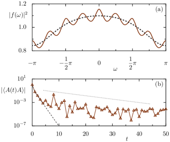
Figure 4: System F at system size $2L=16$. Panel (a) depicts the numerically obtained (thin brown line) and the asymptotic (black dashed line) spectral function. Panel (b) shows the corresponding autocorrelation functions (brown triangles connected by a thin line) and the asymptotic autocorrelation functions $\alpha\lambda_{+}^{t}$ ($t\geq 1$) (black dashed line). The dotted black line indicates the asymptotically slowest possible decay proportional to $\lambda_{-}^{t}$.

Figure 5: Difference $\Delta_{|f|^{2}}$ of the spectral function and its asymptotic value versus system size $L$. The lines connecting the symbols serve as a guide to the eye.

Despite the good agreement between the numerically obtained spectral function with the asymptotic expression we find deviations at finite system size. These deviations become visible in Fig. 2(b), which shows a magnification of panel (a), and are particularly evident for system D. We analyse such finite size deviations in the following in more detail by relating them to the dynamics of autocorrelation functions at intermediate time scales $\lfloor L/2\rfloor<t<T^{*}$, i.e., when $T^{*}>L/2$. At these times Eq. (20) is not valid and deviations from the exponential decay of autocorrelation functions proportional to $\lambda_{\nu}^{t}$ are possible. That is, there might be a time $t^{*}$ at which $\langle A(t^{*})A\rangle\gg\lambda_{\nu}^{t^{*}}$. Upon Fourier transform this contributes to the spectral function as $2\langle A(t^{*})A\rangle\cos(\omega t^{*})$ leading to oscillations of the spectral function around the asymptotic result proportional to $\cos(\omega t^{*})$. Indeed for system D one finds such a behavior at time $t^{*}=5$ as indicated by the inset for system D in Fig. 3. This explains small oscillations of the numerically obtained spectral function around its asymptotic counterpart. However, this behavior will vanish as soon as $L>2t^{*}$ or is at least shifted to later times and thus would be exponentially suppressed. When studying the spectral function for system D at smaller system sizes (not shown) we find that the behavior described above is not as pronounced as at $2L=16$ and thus may appear for individual values of the system size only. One therefore may ask if the deviations described above can occur systematically.

In fact, we expect systematic deviations when autocorrelations in the opposite direction $-\nu$ decay much slower than in the initial direction $\nu$ as both directions are no longer independent at times $t>L/2$. This corresponds to $|\lambda_{-\nu}|>|\lambda_{\nu}|$, where for the operators investigated here $\nu=+1$. For such a situation, denoted as system F, we report these eigenvalues as well as the coefficient $\alpha$ in Table 1. Both the spectral function and the autocorrelation function is depicted in Fig. 5(a) and (b), respectively. Most prominently, one finds $\langle A(t^{*})A\rangle\gg\lambda_{\nu}^{t^{*}}$ at time $t^{*}=8$ which leads to significant oscillations of the numerically obtained spectral function around the corresponding asymptotic result. A heuristic argument for the occurrence of such phenomena can be given as follows. In the previous section we saw that for slowly decaying autocorrelations the exponential decay proportional to $\lambda_{\nu}^{t}$ approximately continues for times $t>L/2$. Thus in the situation at hand there might be contributions to the autocorrelation function decaying as $\lambda_{-\nu}^{t}$ and thus much slower than $\lambda_{\nu}^{t}$. Ultimately this contribution might dominate the autocorrelation function at some time $t^{*}$ as it is observed in system F. Nevertheless, these contribution should be of the order of $|\lambda_{-\nu}|^{t^{*}}\leq|\lambda_{-\nu}|^{L/2}$ and therefore vanish exponentially with increasing system size as well.

For the numerically accessible system sizes we quantify the deviations of numerically obtained and asymptotic spectral function as well as their scaling with system size. We choose their $\text{L}^{2}$ distance $\Delta_{|f|^{2}}:=\big{\|}|f|^{2}-|f_{\infty}|^{2}\big{\|}_{2}$ as a measure for the deviations. This is shown in Fig. 5 for system sizes $L\in\{3,\ldots,8\}$. For the systems A-E we find these differences to exponentially decrease with increasing system size at an approximately equal rate for the system sizes accessible by exact diagonalization. As discussed above deviations are accidentally larger at $2L=16$ for system D and thus $\Delta_{|f|^{2}}$ does not follow the overall exponential decay at this system size. System A shows a slightly slower decay as well as slightly larger deviations. The latter are dominated by small frequencies $|\omega|\lesssim\pi/L$. For system F, as expected, $\Delta_{|f|^{2}}$ is much larger than for the other systems. Although there is an overall decrease of the deviations with increasing system size, the numerically accessible system sizes are not sufficient to extract the exact scaling and and to ultimately confirm the conjectured exponential decay.

IV.3 Distribution of matrix elements and higher moments

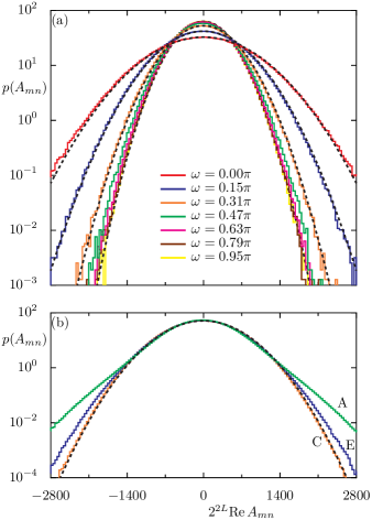
Figure 6: Distribution of real parts of matrix elements for $2L=16$. In panel (a) the distribution for system A at various frequencies (see legend) is shown while (b) depicts distribution of at all frequencies in the system A, C, and D. The black dashed lines show a Gaussian distributions corresponding to the variance determined by (a) $|f(\omega)|^{2}$ at $\omega\in\{0,0.15\pi,0.31\pi,0.95\pi\}$ and (b) $|f(\omega)|^{2}=1$

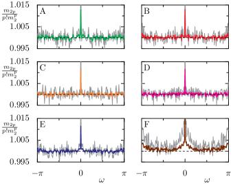
Figure 7: Rescaled fourth (thick colored line) and sixth (thin gray line) moment of the distribution of matrix elements for systems A-F with $2L=16$. The dashed black line corresponds to a Gaussian distribution.

Additionally, we investigate the distribution of matrix elements in systems A-F numerically beyond the second moment. To this end we depict the distribution of real parts of matrix elements of $A$ for various frequencies for system A in Fig. 6(a). Here, we explicitly choose system A as the sharply peaked spectral function indicates that the differences in the distributions are most prominent compared to the systems B-F. Indeed one finds a clearly broader distribution at small frequencies compared to larger frequencies. However, the shape of the distribution for nonzero frequencies is well described by a Gaussian distribution with zero mean represented by dashed lines. At $\omega=0$ the tails of the empirical distribution are slightly underestimated by the corresponding Gaussian distribution. Note that we depict the distribution of matrix elements of $\mathcal{P}_{k}A\mathcal{P}_{k}$ combined for all $k\in\{0,\ldots,L-1\}$ rather than showing the distribution for a fixed $k$ as it increases the number of matrix elements entering the statistics. For this kind of sampling the variance of the Gaussian distribution is given by $q^{-2L}|f(\omega)|^{2}/(2L)$ as it is the marginal distribution of the complex Gaussian distribution of complex matrix elements with twice that variance. For nonzero frequencies the distribution of the imaginary parts of matrix elements (not shown) coincides with that of the real parts. For $\omega=0$, however, one finds an additional peak at $\text{Im}\,A_{mn}=0$ originating from the real diagonal matrix elements.

Moreover, we depict the distribution of real parts of matrix elements not resolved by frequency in Fig. 6(b) for the systems A, C, and D. We do not include systems, B, E, and F as they can not be distinguished from system C on the shown scale. For the almost flat spectral function of system C, $|f(\omega)|^{2}=1$, the resulting distribution is well described by the a Gaussian distribution with variance as discussed above (black dashed line). In contrast for the sharply peaked spectral function of system A the distribution exhibits exponential tails from combining Gaussian distributions with different variances. This deviation from a Gaussian is less pronounced but still visible for system D due to the corresponding spectral function being not flat. Thus, as a non flat spectral function is due the presence of slowly decaying modes, the latter provide an explanation for heavy tails of the distribution of matrix elements, which was observed, for instance, in Ref. RoyLevLui2018 as well.

While the spectral function, i.e., the second moment of the frequency resolved distributions can be computed from the dynamics up to times proportional to the system size, higher moments can not easily be obtained from dynamics up to this time scale. We therefore study higher moments of even order

$$m_{2p}(\omega)=\frac{1}{N(\omega)}\sum_{m,n=0}^{q^{2L}-1}|A_{mn}|^{2p}1_{I_{\Delta}(\omega)}(\omega_{mn})$$ (27)

numerically. Note that Eq. (27) coincides with the variance, Eq. (10), for $p=1$. For a complex Gaussian distribution one has $m_{2p}(\omega)=p\text{!}m_{2}(\omega)^{p}$. Using again the two-site shift invariance of $A$ we compute higher moments of the distribution similarly to the variance. We depict the rescaled moments $m_{2p}(\omega)/(p\text{!}m_{2}(\omega)^{p})$ obtained by this procedure for system A-F in Fig. 7 for $p=2$ (thick colored lines) and $p=3$ (thin gray lines) respectively. Up to small fluctuations they reproduce the Gaussian value of one well for frequencies $|\omega|\gtrsim\pi/L$ further confirming the Gaussian shape of the distribution of matrix elements. Slight deviations appear for small frequencies and partially around $\omega=\pm\pi$. Interestingly the deviations are largest for system F which we cannot readily explain by the dynamics of autocorrelation functions. Note that an accurate estimation of higher moments requires larger and larger system sizes and is not attempted here.

V Conclusions

We study statistics of matrix elements for a class of operators in dual-unitary quantum circuits. For these operators we derive the asymptotic, large $L$, form of the spectral function, i.e., the second moment of the frequency resolved distribution of their matrix elements. This is achieved by utilizing the space-time dual-unitarity of the considered quantum circuits in order to compute the exact short time dynamics of autocorrelation functions. The latter is determined by the local gates in terms of the CPTP maps $\mathcal{M}_{\nu}$. Consequently, their spectrum allows for characterizing the asymptotic properties of spectral functions. More precisely, the presence of slowly decaying modes corresponding to large eigenvalues of $\mathcal{M}_{\nu}$ may lead to sharply peaked spectral functions, whose peak height is inversely proportional to the decay rate of theses modes independent of system size. In contrast, the absence of slowly decaying modes will render the spectral function essentially flat and structureless. In any case, this confirms that the distribution of matrix elements has a variance which is exponentially small in system size as it is implied by the ETH ansatz (1).

Comparing the asymptotic results with spectral functions obtained from exact diagonalization of one dimensional chains of qubits we find excellent agreement for generic dual unitary systems. Additionally, by studying the initial dynamics of autocorrelation functions we confirm the correspondence between the structure of spectral functions and the rate of relaxation of correlations towards their equilibrium value. This reveals the origin of the deviations between numerically obtained spectral functions and its asymptotic form due to the autocorrelation functions at intermediate times. Exact diagonalization also allows for studying the frequency resolved distribution of matrix elements in more detail. In particular, by computing higher moments of the distribution we confirm that the latter is well described by a Gaussian. When disregarding the frequency dependence we find the combined distribution to deviate from a Gaussian distribution. That is, the distribution exhibits exponential tails if the spectral function of the corresponding operator is not flat due to slowly decaying modes.

We emphasize that the computation of the asymptotic spectral function from exact dynamical correlations for initial times via the CPTP maps $\mathcal{M}_{\nu}$ can be straightforwardly extended to a larger class of operators built from extensive sums of local operators. For example, this includes operators supported on both the even and the odd sublattice as well as operators, which violate translational invariance by choosing different nontrivial local operators at different sites. In principle also inhomogeneous dual-unitary quantum circuits in which the local gates depend on the lattice site can be treated similarly. In the latter cases, however, the characterization of spectral functions by the spectrum of a single CPTP map $\mathcal{M}_{\nu}$ can no longer be applied directly.

Although the construction of the asymptotic spectral function presented here agrees well with numerical results in many cases, there may be deviations as discussed above. These deviations are due to autocorrelation functions fluctuating around the exponential decay at intermediate times. Controlling those fluctuations, i.e. rigorously proving that the spectral functions converge towards the asymptotic result, requires knowledge of the dynamics of autocorrelation functions for much larger times, i.e. up to Heisenberg time. This would allow for exactly computing also higher moments of the distribution of matrix elements in order to confirm their Gaussian shape. Computing dynamical correlations at large times exactly is currently out of the scope of the methods based on dual-unitarity presented here and is an important challenge for future work. In contrast, the question whether the asymptotic form of the spectral function gives an accurate description also for generic, i.e., nondual-unitary Floquet circuits may be checked within the perturbative framework of Ref. KosBerPro2021 .

Table 2: Parameters of the local gates for systems A-F.

	$\qquad\qquad\quad\quad\quad u_{\pm,i}$ and $v_{\pm,i}$
A	$u_{+,1}$ = $\left(\begin{smallmatrix}-0.03440376+\text{i}0.95921874&0.10038637+\text{i}0.26198924\\ 0.21897117+\text{i}0.17540641&-0.92413009-\text{i}0.25936037\end{smallmatrix}\right)$
	$u_{-,1}$ = $\left(\begin{smallmatrix}0.79008463+\text{i}0.42675293&-0.3923305-\text{i}0.19931128\\ 0.43912594-\text{i}0.02857657&0.89432201-\text{i}0.08086989\end{smallmatrix}\right)$
	$v_{+,1}$ = $\left(\begin{smallmatrix}-0.48395602-\text{i}0.26977298&-0.38316526+\text{i}0.73904905\\ 0.83244561-\text{i}0.00658885&0.02112852+\text{i}0.55366459\end{smallmatrix}\right)$
	$v_{-,1}$ = $\left(\begin{smallmatrix}0.93026558-\text{i}0.19510379&-0.06303577+\text{i}0.30424817\\ 0.25892305-\text{i}0.17175364&-0.16517923-\text{i}0.93604239\end{smallmatrix}\right)$
	$u_{+,2}$ = $\left(\begin{smallmatrix}0.59082918+\text{i}0.75484878&-0.25218615-\text{i}0.13238709\\ 0.07482491-\text{i}0.27481891&-0.15030173-\text{i}0.9467234\end{smallmatrix}\right)$
	$u_{-,2}$ = $\left(\begin{smallmatrix}-0.09222418+\text{i}0.39020893&0.68968198-\text{i}0.60296804\\ -0.17004669+\text{i}0.90017543&-0.28957816+\text{i}0.27733157\end{smallmatrix}\right)$
	$v_{+,2}$ = $\left(\begin{smallmatrix}-0.04850466+\text{i}0.19938165&0.71066198+\text{i}0.67294413\\ 0.67865799-\text{i}0.70520748&0.05770763+\text{i}0.19691514\end{smallmatrix}\right)$
	$v_{-,2}$ = $\left(\begin{smallmatrix}0.79745641+\text{i}0.20004401&-0.09160851-\text{i}0.56183054\\ 0.54323348+\text{i}0.1701266&0.08528023+\text{i}0.81772955\end{smallmatrix}\right)$
B	$u_{+,1}$ = $\left(\begin{smallmatrix}0.62703598+\text{i}0.33406795&0.07672879-\text{i}0.69952639\\ -0.20388687+\text{i}0.67353888&-0.70782966+\text{i}0.06125921\end{smallmatrix}\right)$
	$u_{-,1}$ = $\left(\begin{smallmatrix}0.16747675-\text{i}0.16925005&0.08962712-\text{i}0.9670951\\ 0.76752061+\text{i}0.59516222&-0.23801086+\text{i}0.00669881j\end{smallmatrix}\right)$
	$v_{+,1}$ = $\left(\begin{smallmatrix}0.7677496-\text{i}0.2283061&-0.30161091+\text{i}0.51717281\\ -0.10473253-\text{i}0.58946412&-0.6418985-\text{i}0.47909233\end{smallmatrix}\right)$
	$v_{-,1}$ = $\left(\begin{smallmatrix}-0.12026078-\text{i}0.76763149&-0.0356572+\text{i}0.62849646\\ 0.02944216+\text{i}0.62881825&-0.12784369+\text{i}0.76640509\end{smallmatrix}\right)$
	$u_{+,2}$ = $\left(\begin{smallmatrix}-0.14548208-\text{i}0.62605359&-0.33929403-\text{i}0.68685619\\ -0.74570464+\text{i}0.17554615&0.57544002-\text{i}0.28631612\end{smallmatrix}\right)$
	$u_{-,2}$ = $\left(\begin{smallmatrix}-0.8076974+\text{i}0.0317134&0.09645005-\text{i}0.58078959\\ 0.42100956+\text{i}0.411546&0.6703337-\text{i}0.45170074\end{smallmatrix}\right)$
	$v_{+,2}$ = $\left(\begin{smallmatrix}-0.20957887-\text{i}0.87909618&0.42114439-\text{i}0.07683755\\ -0.39442252-\text{i}0.16642561&-0.39541195+\text{i}0.81263939\end{smallmatrix}\right)$
	$v_{-,2}$ = $\left(\begin{smallmatrix}-0.01618801-\text{i}0.74304507&0.17034723-\text{i}0.64699597\\ -0.63284003+\text{i}0.21710705&0.7422453-\text{i}0.03807824\end{smallmatrix}\right)$
C	$u_{+,1}$ = $\left(\begin{smallmatrix}0.90604057-\text{i}0.422824846&0.00309542+\text{i}0.01732210\\ 0.01759003-\text{i}0.000477204&0.23054939-\text{i}0.97290150\end{smallmatrix}\right)$
	$u_{-,1}$ = $\left(\begin{smallmatrix}0.77125325+\text{i}0.38295162&0.09729126-\text{i}0.49904999\\ -0.47399433-\text{i}0.18397243&0.08759601-\text{i}0.85662737\end{smallmatrix}\right)$
	$v_{+,1}$ = $\left(\begin{smallmatrix}-0.03365264+\text{i}0.77810214&-0.61909468-\text{i}0.10072905\\ -0.30046665-\text{i}0.55058546&-0.72284161+\text{i}0.28995766\end{smallmatrix}\right)$
	$v_{-,1}$ = $\left(\begin{smallmatrix}0.30726796+\text{i}0.91457831&0.07859757+\text{i}0.250909\\ 0.15206588-\text{i}0.2144968&-0.57405409+\text{i}0.77545406\end{smallmatrix}\right)$
	$u_{+,2}$ = $\left(\begin{smallmatrix}0.02626481-\text{i}0.66133538&0.25064262+\text{i}0.70648705\\ -0.56068151+\text{i}0.49757604&-0.29640378+\text{i}0.59177625\end{smallmatrix}\right)$
	$u_{-,2}$ = $\left(\begin{smallmatrix}0.42871255-\text{i}0.60589777&0.17130354-\text{i}0.64788004\\ -0.63831457-\text{i}0.20407829&0.74138121-\text{i}0.03550296\end{smallmatrix}\right)$
	$v_{+,2}$ = $\left(\begin{smallmatrix}-0.72864047+\text{i}0.07157325&-0.13536488-\text{i}0.66756025\\ 0.23703899+\text{i}0.63857095&0.65682528-\text{i}0.32345048\end{smallmatrix}\right)$
	$v_{-,2}$ = $\left(\begin{smallmatrix}0.53434982+\text{i}0.83729925&-0.04025722+\text{i}0.10853384\\ -0.04081908-\text{i}0.10832378&-0.530004+\text{i}0.84005686\end{smallmatrix}\right)$
D	$u_{+,1}$ =$\left(\begin{smallmatrix}-0.26603916+\text{i}0.20065589&0.25447586-\text{i}0.90785594\\ -0.13280177-\text{i}0.93344741&-0.23732232-\text{i}0.23391823\end{smallmatrix}\right)$
	$u_{-,1}$ = $\left(\begin{smallmatrix}-0.31678703+\text{i}0.71576576&-0.2903863+\text{i}0.55045541\\ -0.20823062-\text{i}0.58648561&0.21059044+\text{i}0.7538742\end{smallmatrix}\right)$
	$v_{+,1}$ = $\left(\begin{smallmatrix}0.13185177+\text{i}0.56539638&-0.53320444+\text{i}0.6153333\\ -0.44095663-\text{i}0.68447008&-0.21038103+\text{i}0.54110792\end{smallmatrix}\right)$
	$v_{-,1}$ = $\left(\begin{smallmatrix}-0.22733824-\text{i}0.12247527&0.77384188-\text{i}0.57834755\\ 0.95104606+\text{i}0.16978966&0.14824766-\text{i}0.21143675\end{smallmatrix}\right)$
	$u_{+,2}$ = $\left(\begin{smallmatrix}0.0780634-\text{i}0.75379364&-0.48091017-\text{i}0.44093839\\ -0.36269368-\text{i}0.5423601&0.75689899+\text{i}0.03745222\end{smallmatrix}\right)$
	$u_{-,2}$ = $\left(\begin{smallmatrix}-0.55448735-\text{i}0.59148658&0.07652242-\text{i}0.58037206\\ -0.5333239-\text{i}0.24135663&0.20968476+\text{i}0.78316339\end{smallmatrix}\right)$
	$v_{+,2}$ = $\left(\begin{smallmatrix}0.44833607+\text{i}0.08778421&-0.87730783-\text{i}0.14703629\\ 0.1319658-\text{i}0.87970093&0.05541789-\text{i}0.4534756\end{smallmatrix}\right)$
	$v_{-,2}$ = $\left(\begin{smallmatrix}-0.23188006-\text{i}0.18849329&-0.78944085-\text{i}0.53617634\\ -0.92453077+\text{i}0.23652648&0.28207876-\text{i}0.09863901\end{smallmatrix}\right)$
E	$u_{+,1}$ = $\left(\begin{smallmatrix}-0.69009297-\text{i}0.51913828&0.25897705+\text{i}0.43266387\\ -0.27973694+\text{i}0.4195406&-0.71455207+\text{i}0.48492082\end{smallmatrix}\right)$
	$u_{-,1}$ = $\left(\begin{smallmatrix}-0.69760973-\text{i}0.58813487&-0.12169375+\text{i}0.39067719\\ 0.04608958+\text{i}0.40658798&-0.79572569+\text{i}0.44652278\end{smallmatrix}\right)$
	$v_{+,1}$ = $\left(\begin{smallmatrix}-0.25224681+\text{i}0.19387489&0.41058323-\text{i}0.85452062\\ -0.92062667-\text{i}0.2263418&-0.31001755+\text{i}0.07144959\end{smallmatrix}\right)$
	$v_{-,1}$ = $\left(\begin{smallmatrix}-0.5888309+\text{i}0.80721348&-0.0176661-\text{i}0.03704691\\ 0.0128777+\text{i}0.03897088&0.98364188+\text{i}0.17539693\end{smallmatrix}\right)$
	$u_{+,2}$ = $\left(\begin{smallmatrix}0.62249645-\text{i}0.54363084&0.37530331-\text{i}0.41965594\\ -0.47107465-\text{i}0.30830563&0.74192191+\text{i}0.36412662\end{smallmatrix}\right)$
	$u_{-,2}$ = $\left(\begin{smallmatrix}-0.52416883-\text{i}0.60807282&0.5702951-\text{i}0.17394819\\ -0.22456187-\text{i}0.5523282&-0.80246836-\text{i}0.02345336\end{smallmatrix}\right)$
	$v_{+,2}$ = $\left(\begin{smallmatrix}0.06282152-\text{i}0.88049157&0.28027461-\text{i}0.37713949\\ -0.19875302-\text{i}0.4257761&-0.1154322+\text{i}0.87514991\end{smallmatrix}\right)$
	$v_{-,2}$ = $\left(\begin{smallmatrix}-0.27681465-\text{i}0.34651419&0.79328171-\text{i}0.4171399\\ -0.8537797+\text{i}0.27269357&0.05274891+\text{i}0.44035893\end{smallmatrix}\right)$
F	$u_{+,1}$ = $\left(\begin{smallmatrix}0.16746295+\text{i}0.04160119&-0.20111797+\text{i}0.96424948\\ 0.922572-\text{i}0.34508898&-0.06652765-\text{i}0.15921235\end{smallmatrix}\right)$
	$u_{-,1}$ = $\left(\begin{smallmatrix}0.0898646-\text{i}0.17188414&-0.51690372+\text{i}0.83378099\\ -0.57135113-\text{i}0.79745726&-0.1011261-\text{i}0.16550926\end{smallmatrix}\right)$
	$v_{+,1}$ = $\left(\begin{smallmatrix}0.78159121+\text{i}0.00257971&0.59336816-\text{i}0.19241296\\ 0.04639178+\text{i}0.62205814&-0.29810347-\text{i}0.72251353\end{smallmatrix}\right)$
	$v_{-,1}$ = $\left(\begin{smallmatrix}0.49866995-\text{i}0.4247034&0.56551407-\text{i}0.50114782\\ -0.65449515-\text{i}0.37761277&0.57368381+\text{i}0.31611957\end{smallmatrix}\right)$
	$u_{+,2}$ = $\left(\begin{smallmatrix}-0.11310322-\text{i}0.90210917&-0.15532151-\text{i}0.3863702\\ 0.07901707+\text{i}0.40885573&-0.39416074-\text{i}0.81928664\end{smallmatrix}\right)$
	$u_{-,2}$ = $\left(\begin{smallmatrix}0.52536851-\text{i}0.10764508&-0.46311121+\text{i}0.70564047\\ 0.84328645+\text{i}0.03561493&0.39396061-\text{i}0.36386065\end{smallmatrix}\right)$
	$v_{+,2}$ = $\left(\begin{smallmatrix}0.44050915-\text{i}0.09668913&-0.71513996+\text{i}0.53402035\\ 0.83571067-\text{i}0.31335375&0.31932476-\text{i}0.31847888\end{smallmatrix}\right)$
	$v_{-,2}$ = $\left(\begin{smallmatrix}0.04940901+\text{i}0.23028099&-0.04022617+\text{i}0.97103618\\ 0.41163049-\text{i}0.88039182&-0.14993899+\text{i}0.18162843\end{smallmatrix}\right)$

Appendix A Moments for two-site shift invariant operators

Here we derive Eq. (12) and its generalization to higher moments for operators obeying two-site shift invariance, i.e., $\left[A,\mathcal{T}^{2}\right]=0$. That is, we are aiming to express $m_{2p}(\omega)$ by the corresponding moments $m_{2p}^{(k)}(\omega)$ of the distribution of matrix elements of $\mathcal{P}_{k}A\mathcal{P}_{k}$ within the momentum $k$ subspace. The basis of this subspace, in which the matrix elements $(\mathcal{P}_{k}A\mathcal{P}_{k})_{mn}$ are computed, is given by the eigenvectors $\ket{n}\in\mathcal{H}$ of $\mathcal{U}$ with $\mathcal{P}_{k}\ket{n}=\ket{n}$, i.e. $k_{n}=k$. More precisely, one has

$$m_{2p}^{(k)}(\omega)=\frac{1}{N_{k}(\omega)}\sum_{m,n=0}^{q^{2L}-1}|\left(\mathcal{P}_{k}A\mathcal{P}_{k}\right)_{mn}|^{2p}1_{I_{\Delta}(\omega)}(\omega_{mn}).$$ (28)

The normalization is given by

$$N_{k}(\omega)=\frac{\Delta q^{4L}}{2\pi L^{2}}=\frac{N(\omega)}{L^{2}}.$$ (29)

as the momentum $k$ subspace asymptotically has dimension $q^{2L}/L$ PinPro2007 . Note that the sum (28) can be taken over all $m,n\in\{0,\ldots q^{2L-1}\}$ as the matrix element $(\mathcal{P}_{k}A\mathcal{P}_{k})_{mn}$ is nonzero only if $k_{m}=k_{n}=k$. Fixing arbitrary $m,n\in\{0,\ldots,q^{2L-1}\}$ this yields

$$|A_{mn}|^{2p} =\Big{|}\sum_{k=0}^{L-1}\bra{m}\mathcal{P}_{k}A\mathcal{P}_{k}\ket{n}\Big{|}^{2p}$$ (30)

$$=\sum_{k=0}^{L-1}|(\mathcal{P}_{k}A\mathcal{P}_{k})_{mn}|^{2p},$$ (31)

where we used $A=\sum_{k=0}^{L-1}\mathcal{P}_{k}A\mathcal{P}_{k}$. Inserting Eq. (31) into Eq. (27) finally gives

$$m_{2p}(\omega) =\frac{1}{N(\omega)}\sum_{m,n=0}^{q^{2L}-1}\sum_{k=0}^{L-1}|\left(\mathcal{P}_{k}A\mathcal{P}_{k}\right)_{mn}|^{2}1_{I_{\Delta}(\omega)}(\omega_{mn})$$ (32)

$$=\frac{1}{L^{2}}\!\sum_{k=0}^{L-1}\frac{L^{2}}{N(\omega)}\!\sum_{m,n=0}^{q^{2L}-1}\!|\left(\mathcal{P}_{k}A\mathcal{P}_{k}\right)_{mn}|^{2}1_{I_{\Delta}(\omega)}(\omega_{mn})$$ (33)

$$=\frac{1}{L^{2}}\sum_{k=0}^{L-1}m_{2p}^{(k)}(\omega),$$ (34)

which corresponds to Eq. (10) for $p=1$ and allows for efficiently computing also higher moments of the distribution of matrix elements.

Appendix B Asymptotical spectral function for eigenvectors of $\mathcal{M}_{\nu}$,

In this section we briefly sketch the derivation of the asymptotical spectral function, Eq. (23), when $a$ in Eq. (18) is an hermitian eigenvector of the CPTP map $\mathcal{M}_{\nu}$ with real eigenvalue $\lambda$. We write $\lambda=\exp(\text{i}\theta-\gamma)$ with $\theta\in\{0,\pi\}$ and $\gamma>0$, which yields $\text{tr}\left(\mathcal{M}_{\nu}^{t}(a)a\right)/q=\exp(\left[\text{i}\theta-\gamma\right]t)$. The Fourier transform, Eq. (22), can then be evaluated as a geometric series (omitting the dependence on $a$) as

$$|f_{\infty}(\omega)|^{2} =1+\sum_{t=1}^{\infty}\text{e}^{\left[\text{i}(\theta+\omega)-\gamma\right]t}+\text{e}^{\left[\text{i}(\theta-\omega)-\gamma\right]t}$$ (35)

$$=\frac{1}{1-\text{e}^{\text{i}(\theta+\omega)-\gamma}}+\frac{1}{1-\text{e}^{\text{i}(\theta-\omega)-\gamma}}-1$$ (36)

$$=\frac{1-\text{e}^{2(\text{i}\theta-\gamma)}}{1+\text{e}^{2(\text{i}\theta-\gamma)}-\text{e}^{\text{i}(\theta+\omega)-\gamma}-\text{e}^{\text{i}(\theta-\omega)-\gamma}}$$ (37)

$$=\frac{\text{e}^{-\text{i}\theta+\gamma}-\text{e}^{\text{i}\theta-\gamma}}{\text{e}^{-\text{i}\theta+\gamma}+\text{e}^{\text{i}\theta-\gamma}-\text{e}^{\text{i}\omega}-\text{e}^{-\text{i}\omega}}$$ (38)

$$=\frac{\sinh(\text{i}\theta-\gamma)}{\cos(\omega)-\cosh(\text{i}\theta-\gamma)},$$ (39)

from which Eq. (23) follows by distinguishing the cases $\theta=0$, corresponding to $\text{sign}(\lambda)=1$, and $\theta=\pi$, corresponding to $\text{sign}(\lambda)=-1$, respectively.

Appendix C Parameters of local gates

In Table (2) we report the matrices $u_{\pm},v_{\pm}\in\text{U}(2)$ entering Eq. (24) for both half steps $i\in\{1,2\}$ for the systems A-F.

References

- (1) J. v. Neumann, Beweis des Ergodensatzes und des H-Theorems in der neuen Mechanik, Zeitschrift für Physik 57, 30 (1929).
- (2) J. M. Deutsch, Quantum statistical mechanics in a closed system, PhysRevA 43, 2046 (1991).
- (3) M. Srednicki, Chaos and quantum thermalization, Phys. Rev. E 50, 888 (1994).
- (4) M. Srednicki, The approach to thermal equilibrium in quantized chaotic systems, J. Phys. A 32, 1163 (1999).
- (5) P. Reimann, Eigenstate thermalization: Deutsch’s approach and beyond, NJP 17, 055025 (2015).
- (6) L. D’Alessio, Y. Kafri, A. Polkovnikov, and M. Rigol, From quantum chaos and eigenstate thermalization to statistical mechanics and thermodynamics, Adv. Phys. 65, 239 (2016).
- (7) J. M. Deutsch, Eigenstate thermalization hypothesis, RepProgPhys 81, 082001 (2018).
- (8) T. Mori, T. N. Ikeda, E. Kaminishi, and M. Ueda, Thermalization and prethermalization in isolated quantum systems: A theoretical overview, J. Phys. B 51, 112001 (2018).
- (9) M. Greiner, O. Mandel, T. W. Hänsch, and I. Bloch, Collapse and revival of the matter wave field of a Bose – Einstein condensate, Nature 419, 51 (2002).
- (10) S. Trotzky, Y.-A. Chen, A. Flesch, I. P. McCulloch, U. Schollwöck, J. Eisert, and I. Bloch, Probing the relaxation towards equilibrium in an isolated strongly correlated one-dimensional Bose gas, Nature Physics 8, 325 (2012).
- (11) T. Kinoshita, T. Wenger, and D. S. Weiss, A quantum newton’s cradle, Nature 440, 900 (2006).
- (12) M. Gring, M. Kuhnert, T. Langen, T. Kitagawa, B. Rauer, M. Schreitl, I. Mazets, D. A. Smith, E. Demler, and J. Schmiedmayer, Relaxation and prethermalization in an isolated quantum system, Science 337, 1318 (2012).
- (13) T. Langen, S. Erne, R. Geiger, B. Rauer, T. Schweigler, M. Kuhnert, W. Rohringer, I. E. Mazets, T. Gasenzer, and J. Schmiedmayer, Experimental observation of a generalized gibbs ensemble, Science 348, 207 (2015).
- (14) M. Schreiber, S. S. Hodgman, P. Bordia, H. P. Lüschen, M. H. Fischer, R. Vosk, E. Altman, U. Schneider, and I. Bloch, Observation of many-body localization of interacting fermions in a quasirandom optical lattice, Science 349, 842 (2015).
- (15) J.-y. Choi, S. Hild, J. Zeiher, P. Schauß, A. Rubio-Abadal, T. Yefsah, V. Khemani, D. A. Huse, I. Bloch, and C. Gross, Exploring the many-body localization transition in two dimensions, Science 352, 1547 (2016).
- (16) A. M. Kaufman, M. E. Tai, A. Lukin, M. Rispoli, R. Schittko, P. M. Preiss, and M. Greiner, Quantum thermalization through entanglement in an isolated many-body system, Science 353, 794 (2016).
- (17) C. Neill, P. Roushan, M. Fang, Y. Chen, M. Kolodrubetz, Z. Chen, A. Megrant, R. Barends, B. Campbell, B. Chiaro, A. Dunsworth, E. Jeffrey, J. Kelly, J. Mutus, P. J. J. O’Malley, C. Quintana, D. Sank, A. Vainsencher, J. Wenner, T. C. White, A. Polkovnikov, and J. M. Martinis, Ergodic dynamics and thermalization in an isolated quantum system, Nature Physics 12, 1037 (2016).
- (18) Y. Tang, W. Kao, K.-Y. Li, S. Seo, K. Mallayya, M. Rigol, S. Gopalakrishnan, and B. L. Lev, Thermalization near integrability in a dipolar quantum newton’s cradle, Phys. Rev. X 8, 021030 (2018).
- (19) D. Bluvstein, A. Omran, H. Levine, A. Keesling, G. Semeghini, S. Ebadi, T. T. Wang, A. A. Michailidis, N. Maskara, W. W. Ho, S. Choi, M. Serbyn, M. Greiner, V. Vuletić, and M. D. Lukin, Controlling quantum many-body dynamics in driven Rydberg atom arrays, Science 10.1126/science.abg2530 (2021).
- (20) G. Biroli, C. Kollath, and A. M. Läuchli, Effect of rare fluctuations on the thermalization of isolated quantum systems, Phys. Rev. Lett. 105, 250401 (2010).
- (21) J. D. Noh, Eigenstate thermalization hypothesis and eigenstate-to-eigenstate fluctuations, arXiv:2008.09318 (2021).
- (22) M. Brenes, T. LeBlond, J. Goold, and M. Rigol, Eigenstate thermalization in a locally perturbed integrable system, Phys. Rev. Lett. 125, 070605 (2020).
- (23) T. LeBlond and M. Rigol, Eigenstate thermalization for observables that break Hamiltonian symmetries and its counterpart in interacting integrable systems, Phys. Rev. E 102, 062113 (2020).
- (24) W. Beugeling, R. Moessner, and M. Haque, Off-diagonal matrix elements of local operators in many-body quantum systems, Phys. Rev. E 91, 012144 (2015).
- (25) C. Schönle, D. Jansen, F. Heidrich-Meisner, and L. Vidmar, Eigenstate thermalization hypothesis through the lens of autocorrelation functions, arXiv:2011.13958 (2020).
- (26) D. Jansen, J. Stolpp, L. Vidmar, and F. Heidrich-Meisner, Eigenstate thermalization and quantum chaos in the Holstein polaron model, Phys. Rev. B 99, 155130 (2019).
- (27) J. Richter, A. Dymarsky, R. Steinigeweg, and J. Gemmer, Eigenstate thermalization hypothesis beyond standard indicators: Emergence of random-matrix behavior at small frequencies, Phys. Rev. E 102, 042127 (2020).
- (28) T. LeBlond, K. Mallayya, L. Vidmar, and M. Rigol, Entanglement and matrix elements of observables in interacting integrable systems, Phys. Rev. E 100, 062134 (2019).
- (29) M. Brenes, J. Goold, and M. Rigol, Low-frequency behavior of off-diagonal matrix elements in the integrable XXZ chain and in a locally perturbed quantum-chaotic XXZ chain, Phys. Rev. B 102, 075127 (2020).
- (30) R. Mondaini and M. Rigol, Eigenstate thermalization in the two-dimensional transverse field ising model. II. off-diagonal matrix elements of observables, Phys. Rev. E 96, 012157 (2017).
- (31) M. Rigol, Breakdown of thermalization in finite one-dimensional systems, Phys. Rev. Lett. 103, 100403 (2009).
- (32) S. Roy, Y. B. Lev, and D. J. Luitz, Anomalous thermalization and transport in disordered interacting Floquet systems, Phys. Rev. B 98, 060201(R) (2018).
- (33) I. M. Khaymovich, M. Haque, and P. A. McClarty, Eigenstate thermalization, random matrix theory, and behemoths, Phys. Rev. Lett. 122, 070601 (2019).
- (34) M. Rigol, V. Dunjko, and M. Olshanii, Thermalization and its mechanism for generic isolated quantum systems, Nature 452, 854 (2008).
- (35) L. F. Santos and M. Rigol, Localization and the effects of symmetries in the thermalization properties of one-dimensional quantum systems, Phys. Rev. E 82, 031130 (2010).
- (36) M. Rigol and L. F. Santos, Quantum chaos and thermalization in gapped systems, PhysRevA 82, 011604(R) (2010).
- (37) H. Kim, T. N. Ikeda, and D. A. Huse, Testing whether all eigenstates obey the eigenstate thermalization hypothesis, Phys. Rev. E 90, 052105 (2014).
- (38) R. Mondaini, K. R. Fratus, M. Srednicki, and M. Rigol, Eigenstate thermalization in the two-dimensional transverse field Ising model, Phys. Rev. E 93, 032104 (2016).
- (39) W. Beugeling, R. Moessner, and M. Haque, Finite-size scaling of eigenstate thermalization, Phys. Rev. E 89, 042112 (2014).
- (40) T. Yoshizawa, E. Iyoda, and T. Sagawa, Numerical large deviation analysis of the eigenstate thermalization hypothesis, Phys. Rev. Lett. 120, 200604 (2018).
- (41) R. Steinigeweg, A. Khodja, H. Niemeyer, C. Gogolin, and J. Gemmer, Pushing the limits of the eigenstate thermalization hypothesis towards mesoscopic quantum systems, Phys. Rev. Lett. 112, 130403 (2014).
- (42) M. Mierzejewski and L. Vidmar, Quantitative impact of integrals of motion on the eigenstate thermalization hypothesis, Phys. Rev. Lett. 124, 040603 (2020).
- (43) S. Sugimoto, R. Hamazaki, and M. Ueda, Test of eigenstate thermalization hypothesis based on local random matrix theory, arXiv:2005.06379 (2020).
- (44) C. Nation and D. Porras, Off-diagonal observable elements from random matrix theory: distributions, fluctuations, and eigenstate thermalization, New J. Phys. 20, 103003 (2018).
- (45) A. Dymarsky, Bound on eigenstate thermalization from transport, arXiv:1804.08626 (2018).
- (46) A. Chan, A. De Luca, and J. Chalker, Eigenstate correlations, thermalization, and the butterfly effect, Phys. Rev. Lett. 122, 220601 (2019).
- (47) L. Foini and J. Kurchan, Eigenstate thermalization hypothesis and out of time order correlators, Phys. Rev. E 99, 042139 (2019).
- (48) M. Brenes, S. Pappalardi, M. T. Mitchison, J. Goold, and A. Silva, Out-of-time-order correlations and the fine structure of eigenstate thermalisation, arXiv:2103.01161 (2021).
- (49) D. J. Luitz and Y. Bar Lev, Anomalous thermalization in ergodic systems, Phys. Rev. Lett. 117, 170404 (2016).
- (50) J. Richter, J. Gemmer, and R. Steinigeweg, Impact of eigenstate thermalization on the route to equilibrium, Phys. Rev. E 99, 050104(R) (2019).
- (51) L. Foini, L. F. Cugliandolo, and A. Gambassi, Dynamic correlations, fluctuation-dissipation relations, and effective temperatures after a quantum quench of the transverse field Ising chain, J. Stat. Mech. 2012, P09011 (2012).
- (52) E. Khatami, G. Pupillo, M. Srednicki, and M. Rigol, Fluctuation-dissipation theorem in isolated quantum systems out of equilibrium, J. Phys.: Conf. Ser. 510, 012035 (2014).
- (53) C. Nation and D. Porras, Quantum chaotic fluctuation-dissipation theorem: Effective Brownian motion in closed quantum systems, Phys. Rev. E 99, 052139 (2019).
- (54) J. D. Noh, T. Sagawa, and J. Yeo, Numerical verification of the fluctuation-dissipation theorem for isolated quantum systems, Phys. Rev. Lett. 125, 050603 (2020).
- (55) K. Mallayya and M. Rigol, Heating rates in periodically driven strongly interacting quantum many-body systems, Phys. Rev. Lett. 123, 240603 (2019).
- (56) M. Pandey, P. W. Claeys, D. K. Campbell, A. Polkovnikov, and D. Sels, Adiabatic eigenstate deformations as a sensitive probe for quantum chaos, Phys. Rev. X 10, 041017 (2020).
- (57) D. Sels and A. Polkovnikov, Dynamical obstruction to localization in a disordered spin chain, arXiv:2009.04501 (2020).
- (58) V. Khemani, A. Vishwanath, and D. A. Huse, Operator spreading and the emergence of dissipative hydrodynamics under unitary evolution with conservation laws, Phys. Rev. X 8, 031057 (2018).
- (59) T. Rakovszky, F. Pollmann, and C. W. von Keyserlingk, Diffusive hydrodynamics of out-of-time-ordered correlators with charge conservation, Phys. Rev. X 8, 031058 (2018).
- (60) A. Nahum, S. Vijay, and J. Haah, Operator spreading in random unitary circuits, Phys. Rev. X 8, 021014 (2018).
- (61) A. Chan, A. De Luca, and J. T. Chalker, Eigenstate correlations, thermalization, and the butterfly effect, Phys. Rev. Lett. 122, 220601 (2019).
- (62) B. Bertini, P. Kos, and T. Prosen, Exact correlation functions for dual-unitary lattice models in dimensions, Phys. Rev. Lett. 123, 210601 (2019).
- (63) C. W. von Keyserlingk, T. Rakovszky, F. Pollmann, and S. L. Sondhi, Operator hydrodynamics, OTOCs, and entanglement growth in systems without conservation laws, Phys. Rev. X 8, 021013 (2018).
- (64) B. C. Dias, M. Haque, P. Ribeiro, and P. McClarty, Diffusive operator spreading for random unitary free Fermion circuits, arXiv:2102.09846 (2021).
- (65) A. Chan, A. De Luca, and J. T. Chalker, Solution of a minimal model for many-body quantum chaos, Phys. Rev. X 8, 041019 (2018).
- (66) A. Nahum, J. Ruhman, S. Vijay, and J. Haah, Quantum entanglement growth under random unitary dynamics, Phys. Rev. X 7, 031016 (2017).
- (67) B. Bertini, P. Kos, and T. Prosen, Entanglement spreading in a minimal model of maximal many-body quantum chaos, Phys. Rev. X 9, 021033 (2019).
- (68) B. Skinner, J. Ruhman, and A. Nahum, Measurement-induced phase transitions in the dynamics of entanglement, Phys. Rev. X 9, 031009 (2019).
- (69) T. Rakovszky, F. Pollmann, and C. W. von Keyserlingk, Sub-ballistic growth of Rényi entropies due to diffusion, Phys. Rev. Lett. 122, 250602 (2019).
- (70) S. Gopalakrishnan and A. Lamacraft, Unitary circuits of finite depth and infinite width from quantum channels, Phys. Rev. B 100, 064309 (2019).
- (71) L. Piroli, B. Bertini, J. I. Cirac, and T. Prosen, Exact dynamics in dual-unitary quantum circuits, Phys. Rev. B 101, 094304 (2020).
- (72) B. Bertini, P. Kos, and T. Prosen, Operator entanglement in local quantum circuits I: Chaotic dual-unitary circuits, SciPost Physics 8, 067 (2020).
- (73) B. Bertini, P. Kos, and T. Prosen, Operator entanglement in local quantum circuits II: Solitons in chains of qubits, SciPost Physics 8, 068 (2020).
- (74) K. Klobas, B. Bertini, and L. Piroli, Exact thermalization dynamics in the ”rule 54” quantum cellular automaton, arXiv:2012.12256 (2021).
- (75) B. Bertini and L. Piroli, Scrambling in random unitary circuits: Exact results, Phys. Rev. B 102, 064305 (2020).
- (76) A. Chan, A. De Luca, and J. T. Chalker, Spectral statistics in spatially extended chaotic quantum many-body systems, Phys. Rev. Lett. 121, 060601 (2018).
- (77) P. Kos, M. Ljubotina, and T. Prosen, Many-body quantum chaos: Analytic connection to random matrix theory, Phys. Rev. X 8, 021062 (2018).
- (78) A. J. Friedman, A. Chan, A. De Luca, and J. T. Chalker, Spectral statistics and many-body quantum chaos with conserved charge, Phys. Rev. Lett. 123, 210603 (2019).
- (79) P. Kos, B. Bertini, and T. Prosen, Chaos and ergodicity in extended quantum systems with noisy driving, arXiv:2010.12494 (2020).
- (80) A. Flack, B. Bertini, and T. Prosen, Statistics of the spectral form factor in the self-dual kicked Ising model, Phys. Rev. Research 2, 043403 (2020).
- (81) I. Reid and B. Bertini, Entanglement Barriers in Dual-Unitary Circuits, arXiv:2103.12794 (2020).
- (82) B. Bertini, P. Kos, and T. Prosen, Exact spectral form factor in a minimal model of many-body quantum chaos, Phys. Rev. Lett. 121, 264101 (2018).
- (83) B. Bertini, P. Kos, and T. Prosen, Random matrix spectral form factor of dual-unitary quantum circuits, arXiv:2012.12254 (2021).
- (84) A. Hamma, S. Santra, and P. Zanardi, Quantum entanglement in random physical states, Phys. Rev. Lett. 109, 040502 (2012).
- (85) A. Hamma, S. Santra, and P. Zanardi, Ensembles of physical states and random quantum circuits on graphs, PhysRevA 86, 052324 (2012).
- (86) M. Akila, D. Waltner, B. Gutkin, and T. Guhr, Particle-time duality in the kicked Ising spin chain, J. Phys. A 49, 375101 (2016).
- (87) T. Prosen, General relation between quantum ergodicity and fidelity of quantum dynamics, Phys. Rev. E 65, 036208 (2002).
- (88) P. W. Claeys and A. Lamacraft, Ergodic and non-ergodic dual-unitary quantum circuits with arbitrary local hilbert space dimension, arXiv:2009.03791 (2020).
- (89) P. Kos, B. Bertini, and T. Prosen, Correlations in perturbed dual-unitary circuits: Efficient path-integral formula, Phys. Rev. X 11, 011022 (2021).
- (90) S. A. Rather, S. Aravinda, A. Lakshminarayan, Creating ensembles of dual unitary and maximally entangling quantum evolutions, Phys. Rev. Lett. 125, 070501 (2020).
- (91) S. Aravinda, S. A. Rather, A. Lakshminarayan, From dual-unitary to quantum Bernoulli circuits: Role of the entangling power in constructing a quantum ergodic hierarchy, arXiv:2101.04580 (2021).
- (92) M. Ippoliti, V. Khemani, Postselection-free entanglement dynamics via spacetime duality, arXiv:2010.15840 (2020).
- (93) M. Ippoliti, T. Rakovszky, V. Khemani, Fractal, logarithmic and volume-law entangled non-thermal steady states via spacetime duality, arXiv:2103.06873 (2021).
- (94) A. Lerose, M. Sonner, D. A. Abanin, Influence matrix approach to many-body Floquet dynamics, arXiv:2009.10105 (2020).
- (95) R. Hamazaki, Exceptional Dynamical Phase Transitions in Periodically Driven Quantum Systems, arXiv:2012.11822 (2020).
- (96) T.-C. Lu and T. Grover, Entanglement transitions via space-time rotation of quantum circuits, arXiv:2103.06356 (2021).
- (97) C. Pineda and T. Prosen, Universal and nonuniversal level statistics in a chaotic quantum spin chain, Phys. Rev. E 76, 061127 (2007).