OnionNet-2: A Convolutional Neural Network Model for Predicting Protein-Ligand Binding Affinity based on Residue-Atom Contacting Shells

Abstract

One key task in virtual screening is to accurately predict the binding affinity ($\triangle$$G$) of protein-ligand complexes. Recently, deep learning (DL) has significantly increased the predicting accuracy of scoring functions due to the extraordinary ability of DL to extract useful features from raw data. Nevertheless, more efforts still need to be paid in many aspects, for the aim of increasing prediction accuracy and decreasing computational cost. In this study, we proposed a simple scoring function (called OnionNet-2) based on convolutional neural network to predict $\triangle$$G$. The protein-ligand interactions are characterized by the number of contacts between protein residues and ligand atoms in multiple distance shells. Compared to published models, the efficacy of OnionNet-2 is demonstrated to be the best for two widely used datasets CASF-2016 and CASF-2013 benchmarks. The OnionNet-2 model was further verified by non-experimental decoy structures from docking program and the CSAR NRC-HiQ data set (a high-quality data set provided by CSAR), which showed great success. Thus, our study provides a simple but efficient scoring function for predicting protein-ligand binding free energy.

I Introduction

Protein-ligand binding is the basic of almost all processes in living organismsref1 thus predicting binding affinity($\triangle$$G$) of protein-ligand complex becomes the research focus of bioinformatics and drug design. ref2 ; ref3 ; ref4 Theoretically, molecular dynamics (MD) simulations and free energy calculations (for instance, thermal integration method and free energy perturbation can provide accurate predictions of $\triangle$$G$ relying on extensive configurational sampling and calculation, leading to a large demand in computational cost.ref4 ; ref5 ; ref6 ; ref7 Therefore, developing simple, accurate and efficient scoring methods to predict protein-ligand binding will greatly accelerate the drug design process.ref8 To achieve this, several theoretical methods (scoring functions) have been proposed. Typically, the scoring functions are based on calculations of interactions between protein and ligand atoms.ref1 ; ref8 ; ref9 ; ref10 This includes quantum mechanics calculations, molecular dynamics simulations (electrostatic interaction, van der Waals interaction, hydrogen-bond and etc.), empirical-based interacting models.ref1 ; ref9 ; ref10 ; ref11

In recent years, approaches based on machine learning (ML) have been applied in scoring functions and demonstrated great success.ref12 ; ref13 ; ref14 ; ref15 For instance, RF-Scoreref16 and NNScore are two pioneering ML-based scoring functions.ref17 Compared with classical approaches, these ML-based methods allow higher flexibility in selecting configurational representations or features for protein and ligand. More importantly, these methods have been demonstrated to perform better and more effective than classical approaches.ref18 ; ref19 Recently, the deep learning (DL) approaches have provided alternative solution. Compared with ML, the DL models perform better at learning features from the raw data to extract the relationship between these features and labels.ref20 ; ref21 ; ref22 Thus, DL algorithms have been introduced to model the structure-activity relationships.ref23 ; ref24 ; ref25 One of the most popular methods of DL is the convolutional neural network (CNN), which is a multi-layer perceptron inspired by the neural network of living organisms.ref26

Inspired by the great success of DL and CNN techniques, several models applying CNN to virtual screening and $\triangle$$G$ prediction have been reported.ref27 ; ref28 ; ref29 ; ref30 ; ref31 ; ref32 ; ref33 ; ref34 ; ref35 For example, Öztürk and co-workers reported a DeepDTA model based on one-dimensional (1D) convolution, which took protein sequences and simplified molecular input line entry specification (SMILES) codes of ligand as inputs to predict drug-target $\triangle$$G$.ref30 Using 3D CNN model, two independent groups developed scoring functions, named Pafnucyref31 and K_deepref29 , to model the complex in a cubic box centered on the geometric center of the ligand to predict the $\triangle$$G$ of protein-ligand complex. More interestingly, Russ et al. employed Graph-CNNs to automatically extract features from protein pocket and 2D ligand graphs, and demonstrated that the Graph-CNN framework can achieve superior performance without relying on protein-ligand complexes.ref34 Our group has proposed a 2D convolution-based predictor, called OnionNet, based on element-pair-specific contacts between ligands and protein atoms.ref32 As is shown, these DL and CNN based approaches, achieved higher accuracy in $\triangle$$G$ prediction than most traditional scoring functions, such as AutoDock,ref36 ; ref37 X-Scoreref38 and KScore.ref39

For DL scoring functions, how to treat with the high-dimensional structural information encoded in the 3D structures and convert to the low-dimensional features for ML (or DL) training is critical. For most structure-based ML/DL models, the features are usually derived from the atomic information of proteins and ligands, such as the element type and spatial coordinates of the atom and even other atomic properties.ref29 ; ref31

We noticed that same elements in different residues have quite different physical and chemical properties, which might greatly affect the predicting performance of scoring functions. Considering that the twenty types of amino acids can be treated as intrinsic classifications of protein compounds which involve lay features of them, like polar, apolar, aromatic and etc. We anticipate that it may be more beneficial to encode protein as residues instead of atoms in developing DL scoring functions.

In this work, we proposed a simple OnionNet-2 – a 2D CNN based regression model, which adopts the rotation-free residue-atom-specific contacts in multiple distance shells to describe the protein (residues) - ligand (atoms) interactions. We demonstrated that, our present method can significantly improve the prediction power by about 3.7% than previous models, thus providing an efficient and accurate approach for predicting protein-ligand interactions and uncover a new trend of using DL technique for massive biological structures training for drug design.

II Methods

II.1 Descriptors

The features employed are the pair numbers of the specific residue (protein)-atom (ligand) combination in multiple distance shells. The minimum distances between any atom in the ligand and any residue of protein are treated as the representative distances. First, around each atom in the ligand, we defined N continuously packed shells. The thickness of each shell is $\delta$, except that the first shell is a sphere with a radius of $d_{0}$. The boundary K_i of the $i$th shell is as follows

0 $<$ K_i $<$ $d_{0}$,   $i$ = 1

$d_{0}$ + (i - 2)$\delta$ $\leq$ K_i $<$ $d_{0}$ + (i - 1)$\delta$,   i $\geq$ 2

Meanwhile, we classified atoms in the ligand into eight types, namely C, H, O, N, P, S, HAL and DU, where HAL represents the halogen elements (F, Cl, Br and I), and DU represents the element types excluded in these seven types.

T_e $\in$ {C, H, O, N, P, S, HAL, DU}

When pre-processing the structure file, water and ions were treated explicitly because crystal water molecules and ions could affect the protein-ligand binding.ref40 ; ref41 In addition to the twenty standard residues, we added an expanded type named “OTH” to represent water, ions and any other non-standard residues.

T_r $\in$ {GLY, ALA, VAL, LEU, ILE, PRO, PHE, TYR, TRP, SER, THR, CYS, MET, ASN, GLN, ASP, GLU, LYS, ARG, HIS, OTH }

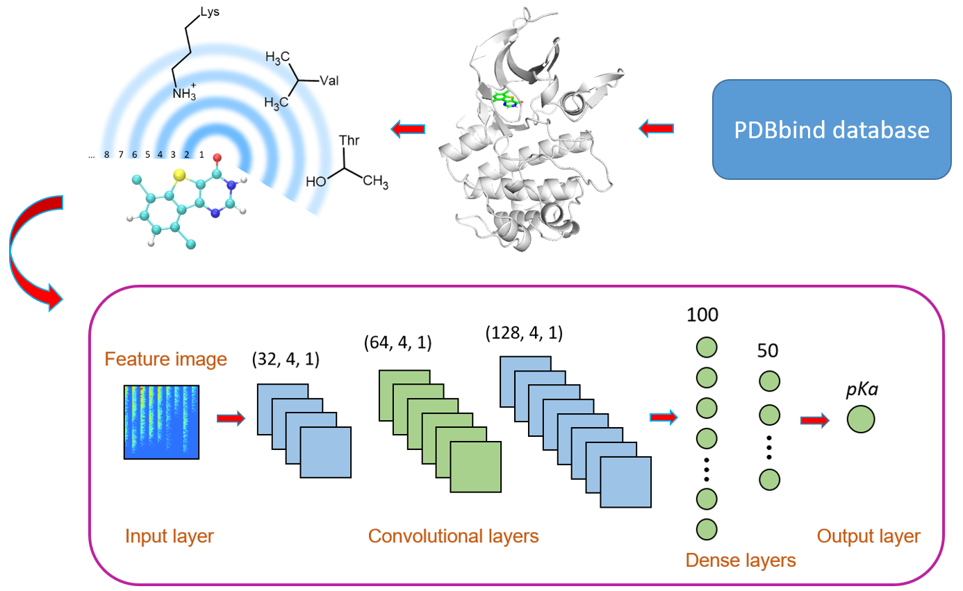
Figure 1: Workflow of OnionNet-2.

It is worth mention that the residue-atom distance is defined as the distance between the atom in the ligand and the nearest heavy atom in the residue. A 2D visual representation is depicted at the upper left of Fig. 1. For any shell, the number of contacts for each residue-atom pair is calculated and used as a feature. Each shell has 8$\times$21=168 residue-atom combinations, which means that there are 168 features for a shell. Thus, if the total number of shells is N, 168$\times$N features will be generated.

$$n_{T_{r},T_{e}}=\sum_{r=1}^{R}\sum_{e=1}^{E}c_{r,e}^{i}$$ (1)

$$c_{r,e}^{i}=\left\{\begin{aligned} \begin{gathered}1,(i-2)\delta+d_{0}\leq d_{r,e}<(i-1)\delta+d_{0}\\ 0,otherwise\end{gathered}\end{aligned}\right.$$ (2)

Here, $R$ is the total number of residues in the protein, and $E$ is the total number of atoms in the ligand. The $d_{r,e}$ is the minimum distance between the residue $r$ in the protein and the atom $e$ in the ligand, and $n_{T_{r},T_{e}}^{i}$ is the number of contacts of the specific residue-element combination in the ith shell. The $c_{r,e}^{i}$ is 1 when $(i-2)\delta+d_{0}\leq d_{r,e}<(i-1)\delta+d_{0}$, otherwise $c_{r,e}^{i}$ is 0. Following our previous study,ref32 we used $d_{0}=1$ Å and $\delta=0.5$ Å. Interestingly such shell-like, or radial, representations of protein environments, have been demonstrated to be superior features in protein function prediction.ref35 The preparation of datasets and the CNN architectureref42 ; ref43 can be found in SI. The source code of OnionNet-2 is available at https://github.com/zchwang/OnionNet-2/.

II.2 Evaluation metrics

To evaluate the performance of the OnionNet-2,we adopted the loss function defined in the previous work.ref32

$$loss=\alpha(1-R)+(1-\alpha)RMSE$$ (3)

$$R=\frac{\sum_{i}^{n}(x_{i}-\bar{x})(y_{i}-\bar{y})}{\sqrt{\sum_{i}^{n}(x_{i}-\bar{x})^{2}\sqrt{\sum_{i}^{n}(y_{i}-\bar{y})^{2}}}}$$ (4)

where R and RMSE represent Pearson correlation coefficient(Eq. 3) and root-mean-squared error, respectively; x_i is the predicted pKa for ith complex; y_i is the experimental pKa of this complex; $\bar{x}$ and $\bar{y}$ are the averages of all predicted values and experimental values.ref44 The $\alpha(0\leq\alpha\leq 1)$ value is an adjustable factor for adjusting the weight with R and RMSE, which was finally set to 0.7. For each independent training task, we adopted early stopping (patience = 20, that is, if the change of the loss value in the validating set is less than 0.001 after 20 epochs, the training is terminated) and save the model that performed best on the validating set. For the prediction in each case, five independently trainings were conducted to obtain the predicted mean value.

III Results and Discussions

III.1 The predictive power of OnionNet-2

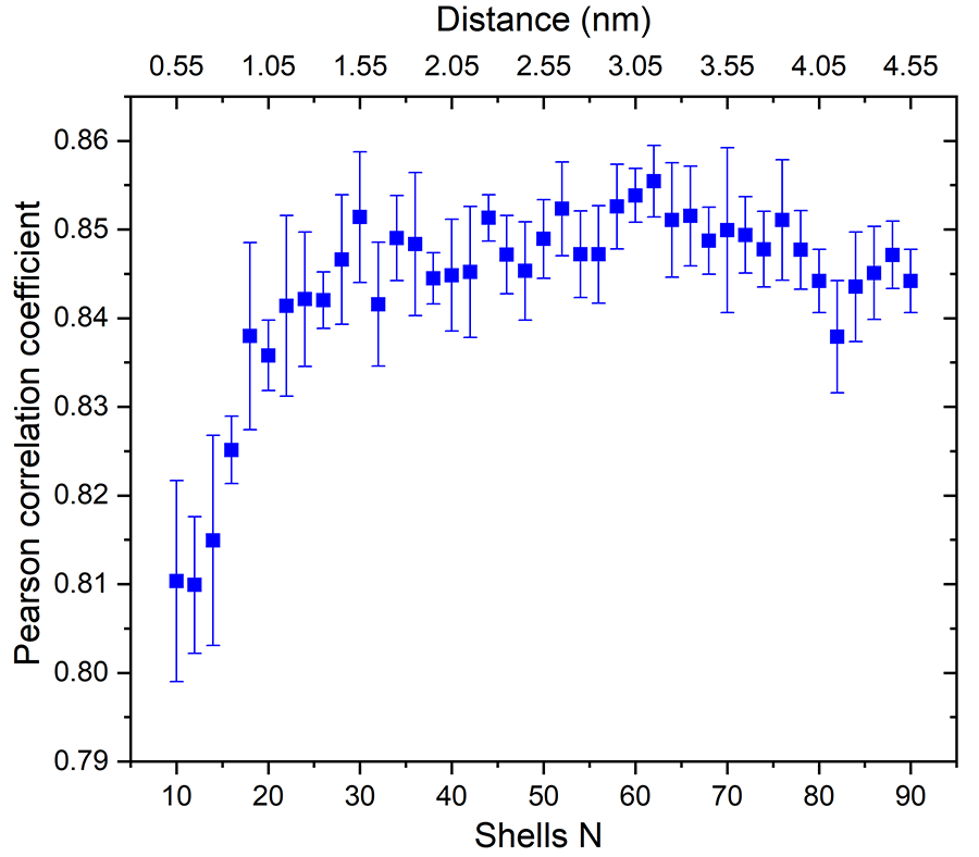
Figure 2: The Pearson correlation coefficient with respect to the shell number N for OnionNet-2 testing with core set v.2016. The bars indicate the standard deviations of the R values for five independent runs.

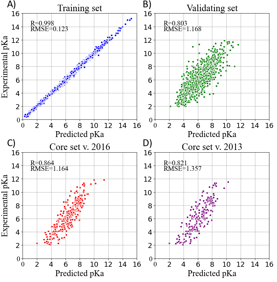
Figure 3: OnionNet-2 predicted pKa with respect to experimental determined pKa on (a) training set, (b) validating set, and two test sets of (c) core set v.2016 and (d) core set v.2013.

Firstly, we explored the effect of shell number N on the predictive capability of the OnionNet-2 model. A range of the total shell number $10\leq N\leq 90$ was tested with interval of 2. According to our definitions of distance shell, this covers a separation between the residue and the atom from 0.55 nm to 4.55 nm. Fig. 2 depicts the trend of the R value to shell number N testing with core set v.2016ref44 . For N from 10 to 20, the R quickly increases as the total number of shells increases. This is expected because as the number of shells increases, the interactions between ligand and protein were gradually captured by the model. The R value reached the first peak for N is 30. This means that OnionNet-2 can achieve high prediction accuracy at a relatively low computational cost. Then, R fluctuates in a range of 0.01 until reaches the global maximum value when N = 62. Fig. 3 summarized the predicted mean pKa, with respect to experimental value, using N=62, on the training set (Fig. 3a), validating set (Fig. 3b) and two testing sets, core set v.2016 (Fig. 3c) and core set v.2013ref45 ; ref46 ; ref47 (Fig. 3d). It shows that the predicted pKa and experimental pKa are highly correlated for the two testing sets and validating set. After this point, R decreases when N increase. We attribute this to the enormous data that leads to the introduction of noise in the training. Unless otherwise specified, we adopted N of 62 in the following discussions. In addition, we also re-trained the model with two elder versions (v.2016 and v.2018) of the PDBbind database, and the R values of our re-trained models are almost the same (Fig. S1 and Table S1).

The performance of some published scoring functionsref48 ; ref49 and OnionNet-2 tested on CASF-2016 and CASF-2013 are showed in Fig. 4 and Fig. S2, respectively. The corresponding R and RMSE (or SD) achieved by these representative scoring functions can be found in Table S2 in SI. Firstly, our OnionNet-2 model achieved highest R of 0.864 and RMSE of 1.164 with the core set v.2016, and R = 0.821 and RMSE = 1.357 with the core set v.2013. These were significantly higher than other scoring functions. The $2^{nd}$ best scoring function was AGL, which adopted the gradient boosting trees (GBTs) algorithm, focusing on multiscale weighted labeled algebraic subgraphs to characterize protein-ligand interactions.ref48 For two 3D convolution-based scoring functions K_deepref29 and Pafnucyref31 , they adopted 3D voxel representation to model the protein-ligand complex and explicitly treated with physical properties of atoms such as hydrophobic, hydrogen-bond donor or acceptor and aromatic etc. into consideration. It is interesting to find that although we only employed the residue-atom contact to mimic the interactions between the protein and the ligand in OnionNet-2, the predicting power is higher. This further reveals that the selected features have a great impact on the predictive power of the CNN-based scoring functions. Secondly, as is expected, the introduction of ML/DL techniques into models has systematically enhanced the predicting accuracy.

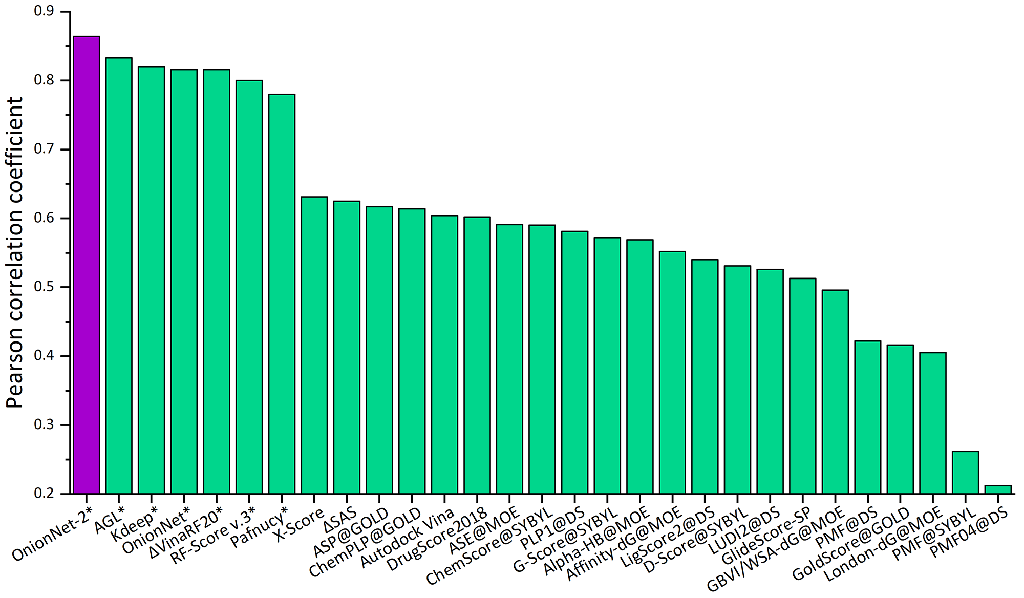
Figure 4: Pearson correlation coefficient of different scoring functions on CASF-2016 benchmark.

III.2 Evaluation of the generalization ability of the model on different test sets

Generally, DL models display a good generalization behavior in practical applications.ref50 To verify the generalization ability of the OnionNet-2, the CSAR NRC-HiQ data set provided by CSARref51 was used as an additional test set in this study. This data set contains two subsets which contain 176 and 167 protein-ligand complexes respectively. For the two previous ML models, K_deep and RF-Score, the researchers used 55 and 49 complexes in two subsets respectively as test data.ref29 To provide a direct comparison with them, we adopted the same data for the OnionNet-2 test. It is worth mention that the two test subsets from the CSAR NRC-HiQ only have two common complexes with core set v.2013, namely 2jdy and 2qmj, and does not overlap with the training set, validation set and core set v.2016. The performance of K_deep, RF-Score and OnionNet-2 on these two subsets are shown in Table I, and the scatter plots of the pKa predicted by OnionNet-2 with respect to experimental pKa can be found in Fig. S3 in SI. As expected, our model achieved a higher performance than K_deep and RF-score. For subset 1, the present OnionNet-2 achieved R of 0.89, which is considerably higher than that of K_deep (0.72) and RF-Score (0.78). This is also true for subset 2. Especially that, the R value of K_deep model is only 0.65 for subset 2, indicating weak predicting capability on these data. These results effectively demonstrated that OnionNet-2 has a good generalization ability.

Table 1: The performance of OnionNet-2, K_deep and RF-Score achieved on subsets from CSAR NRC-HiQ data set

	Subset 1		Subset 2
	R	RMSE	R	RMSE
OnionNet-2	0.89	1.50	0.87	1.21
Kdeepref29	0.72	2.09	0.65	1.92
RF-Scoreref29	0.78	1.99	0.75	1.66

III.3 Evaluations on subsets of non-experimental decoy structures

As all the training and validating sets are composed of well-validated native structures in previous studies, it is largely unknown whether the DL method is capable to distinguish “bad data” that are incorporated in these integrated data sets, for instance, non-native binding poses. To verify this, we tested OnionNet-2 to deal with non-experimental structures (generated by docking programs). Technically, non-native binding poses (called decoys) were generated based on core set v.2016 complexes by AutoDock Vina.ref52 ; ref53 The detailed information of the generation of decoys can be found in the SI.ref54 ; ref55

The predicting accuracy was evaluated by calculating the RMSE between the predicted pKa of the decoy complex and the pKa of the corresponding native receptor-ligand complex which is shown in Fig. 5. It is clear that, the RMSE quickly increased with increasing RMSD. This is expected because decoys with larger RMSD result in more severe change of $\delta$G. These results reveal that OnionNet-2 can accurately respond to changes of the ligand binding poses and distinguish the native structure.

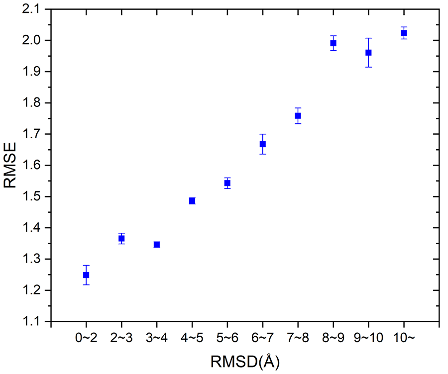
Figure 5: RMSE between the predicted pKa of the decoy complex and the pKa of the corresponding native receptor-ligand complex achieved by OnionNet-2 on different protein-decoy complexes subsets. The bars indicate the standard deviations of RMSE for five independent runs.

Table 2: Pearson correlation coefficients achieved by OnionNet-2 and previous scoring functions on three series of subsets

	Subset H			Subset S			Subset V
	H1	H2	H3	S1	S2	S3	V1	V2	V3
OnionNet-2	0.872	0.866	0.856	0.868	0.839	0.869	0.856	0.774	0.866
$\triangle$VinaRF20*	0.820	0.832	0.804	0.843	0.765	0.823	0.727	0.760	0.818
X-Score*	0.698	0.570	0.661	0.743	0.536	0.572	0.437	0.622	0.579
X-ScoreHS*	0.711	0.565	0.647	0.748	0.557	0.546	0.433	0.630	0.559
$\triangle$SAS*	0.641	0.643	0.589	0.746	0.572	0.494	0.480	0.669	0.541
X-ScoreHP*	0.669	0.558	0.672	0.740	0.510	0.575	0.450	0.575	0.580
AutoDock Vina*	0.626	0.586	0.641	0.745	0.521	0.507	0.484	0.564	0.486

• Results of the last six rows taken from Su et al.ref44

III.4 Effects of hydrophobic scale, buried solvent-accessible area and excluded volume inside the binding pockets on the prediction accuracy

Principally, the physical interactions between protein and ligand determine the $\triangle$$G$. The dominating factors for overall $\triangle$$G$ involve electrostatic interactions, van der Waals interactions, hydrogen bonds, hydration/de-hydration during complexation. However, such mechanistic interactions were not directly input into DL features. At molecular level, these involves the size and shape of the binding pocket, and the nature of residues around the binding pocket which determine its physicochemical characteristics.ref56 Whether DL models can accurately represent the structural specificity of the binding pocket is poorly documented.

The entire CASF-2016 test set can be divided into three subsets by each of three descriptors according to physical classifications of the binding pocket on the target protein.ref44 The three descriptors include H-scale (hydrophobic scale of the binding pocket), $\triangle SAS$ (buried percentage of the solvent-accessible area of the ligand after binding) and $\triangle VOL$ (excluded volume inside the binding pocket after ligand binding). Protein-ligand complexes in CASF-2016 were grouped into 57 clusters, and the authors sorted all 57 clusters in ascending order by each descriptor. Then, these complex clusters were divided into three subsets according to the chosen descriptor, labeled as H1, H2 and H3 or S1, S2 and S3 or V1, V2 and V3. These subsets were used as validations of our OnionNet-2 model. As comparison, previous scoring functions were also tested on these three sets of subsets by Su et al.ref44 , and the results are summarized in Table II.

As can be seen in Table II, OnionNet-2 achieved higher prediction accuracy compared with other soring functions when tested on H-, S- and V-series subsets. This indicates that the feature based on the contact number of residue-atom pairs in multiple shell is capable of capturing the hydrophobic scale of the binding pocket. The number of contacts in different shells (specifically the shells within the binding pocket) may be able to reflect the buried solvent-accessible surface area and the excluded volume of the ligand.

We noticed that, compared to other subsets, the R value of OnionNet-2 on V2 subset is clearly lower than other subsets (nevertheless it is still high than other scoring functions). This may indicate that our model is less sensitive to medium-sized binding pockets. Thus it may be still challenging for current scoring functions to recognize the size and shape of the binding pocket.

Furthermore, we plotted the detailed scatter plots of predicted pKa and experimental pKa in Fig. S4 according to the specific H, S and V range. It is interesting to find almost no dependence of pKa with the values of H, S or V. Thus we speculate that a more realistic descriptor for the ligand characteristic in the binding pocket is essential to guide the protein-ligand $\triangle$$G$ prediction.

IV Conclusion

To summarize, a 2D convolution-based CNN model, OnionNet-2, is proposed for prediction of the protein-ligand binding free energy. The contacting pair numbers between the protein residues and the ligand atoms were used as features for DL training. Using CASF-2013 and CASF-2016 as benchmarks, our model achieved the highest accuracy to predict $\triangle$$G$ than previous scoring functions. In addition, when employing different versions of PDBbind database for training, the performance of OnionNet-2 is nearly the same. The generalization ability of the model was verified by the CSAR NRC-HiQ data set and decoy structures. Our result also indicates that OnionNet-2 has the capability to recognize these physical natures (in detail, hydrophobic scale of the binding pocket, buried percentage of the solvent-accessible area of the ligand upon binding and excluded volume inside the binding pocket upon ligand binding) of the ligand-binding pocket interactions.

- (1) X. Du, Y. Li, Y. L. Xia, S. M. Ai, J. Liang, P. Sang, X. L. Ji, and S. Q. Liu, Int J Mol Sci 17 (2016).
- (2) I. A. Guedes, F. S. S. Pereira, and L. E. Dardenne, Front Pharmacol 9, 1089 (2018).
- (3) O. Guvench and A. D. MacKerell, Jr., Curr Opin Struct Biol 19, 56 (2009).
- (4) S. R. Ellingson, B. Davis, and J. Allen, Biochimica et Biophysica Acta (BBA)-General Subjects 1864, 129545 (2020).
- (5) J. Michel and J. W. Essex, J Comput Aided Mol Des 24, 639 (2010).
- (6) M. K. Gilson and H. X. Zhou, Annu Rev Biophys Biomol Struct 36, 21 (2007).
- (7) N. Hansen and W. F. van Gunsteren, J Chem Theory Comput 10, 2632 (2014).
- (8) J. Liu and R. Wang, J Chem Inf Model 55, 475 (2015).
- (9) S. Y. Huang, S. Z. Grinter, and X. Zou, Phys Chem Chem Phys 12, 12899 (2010).
- (10) S. Z. Grinter and X. Zou, Molecules 19, 10150 (2014).
- (11) N. Huang, Chakrapani Kalyanaraman, John J. Irwin, and Matthew P. Jacobson., J Chem Inf Model 46, 243 (2006).
- (12) Y. C. Lo, S. E. Rensi, W. Torng, and R. B. Altman, Drug Discov Today 23, 1538 (2018).
- (13) J. Vamathevan et al., Nat Rev Drug Discov 18, 463 (2019).
- (14) C. Shen, J. Ding, Z. Wang, D. Cao, X. Ding, and T. Hou, WIREs Computational Molecular Science 10 (2019).
- (15) A. Lavecchia, Drug Discov Today 20, 318 (2015).
- (16) P. J. Ballester and J. B. O. Mitchell, Bioinformatics 26, 1169 (2010).
- (17) J. D. Durrant and J. A. McCammon, J Chem Inf Model 50, 1865 (2010).
- (18) Q. U. Ain, A. Aleksandrova, F. D. Roessler, and P. J. Ballester, Wiley Interdisciplinary Reviews: Computational Molecular Science 5, 405 (2015).
- (19) G. S. Heck, V. O. Pintro, R. R. Pereira, M. B. de Avila, N. M. B. Levin, and W. F. de Azevedo, Curr Med Chem 24, 2459 (2017).
- (20) W. Wang and X. Gao, Methods 166, 1 (2019).
- (21) E. Gawehn, J. A. Hiss, and G. Schneider, Mol Inform 35, 3 (2016).
- (22) H. Chen, O. Engkvist, Y. Wang, M. Olivecrona, and T. Blaschke, Drug Discov Today 23, 1241 (2018).
- (23) K. Yang et al., J Chem Inf Model 59, 3370 (2019).
- (24) R. Winter, F. Montanari, F. Noe, and D. A. Clevert, Chem Sci 10, 1692 (2019).
- (25) F. Ghasemi, A. Mehridehnavi, A. Perez-Garrido, and H. Perez-Sanchez, Drug Discov Today 23, 1784 (2018).
- (26) A. Lavecchia, Drug Discov Today 24, 2017 (2019).
- (27) J. Jimenez, S. Doerr, G. Martinez-Rosell, A. S. Rose, and G. De Fabritiis, Bioinformatics 33, 3036 (2017).
- (28) J. Gomes, B. Ramsundar, K. Fackeldey, and M. S. Pacella, arXiv:1703.10603.
- (29) J. Jiménez, M. škalič, G. Martínez-Rosell and G. De Fabritiis, J Chem Inf Model 58, 287 (2018).
- (30) H. Öztürk, A. Özgür and E. Ozkirimli, Bioinformatics 34, i821 (2018).
- (31) M. M. Stepniewska-Dziubinska, P. Zielenkiewicz, and P. Siedlecki, Bioinformatics 34, 3666 (2018).
- (32) L. Zheng, J. Fan, and Y. Mu, ACS Omega 4, 15956 (2019).
- (33) J. A. Morrone, J. K. Weber, T. Huynh, H. Luo, and W. D. Cornell, J Chem Inf Model 60, 4170 (2020).
- (34) W. Torng and R. B. Altman, J Chem Inf Model 59, 4131 (2019).
- (35) W. Torng, R. B. Altman, and A. Valencia, Bioinformatics 35, 1503 (2019).
- (36) G. M. Morris, D. S. Goodsell, R. S. Halliday, R. Huey, W. E. Hart, R. K. Belew, and A. J. Olson, J Comput Chem 19, 1639 (1998).
- (37) R. Huey, G. M. Morris, A. J. Olson, and D. S. Goodsell, J Comput Chem 28, 1145 (2007).
- (38) R. Wang, L. Lai, and S. Wang, J Comput Aided Mol Des 16, 11 (2002).
- (39) X. Zhao et al., J Chem Inf Model 48, 1438 (2008).
- (40) A. T. Garcia-Sosa, J Chem Inf Model 53, 1388 (2013).
- (41) F. Spyrakis, M. H. Ahmed, A. S. Bayden, P. Cozzini, A. Mozzarelli, and G. E. Kellogg, J Med Chem 60, 6781 (2017).
- (42) M. Abadi et al., in OSDI’16 12th USENIX symposium on operating systems design and implementation2016, pp. 265.
- (43) F. Pedregosa et al., Journal of Machine Learning Research 12, 2825 (2011).
- (44) M. Su, Q. Yang, Y. Du, G. Feng, Z. Liu, Y. Li, and R. Wang, J Chem Inf Model 59, 895 (2019).
- (45) Y. Li, Z. Liu, J. Li, L. Han, J. Liu, Z. Zhao, and R. Wang, J Chem Inf Model 54, 1700 (2014).
- (46) Y. Li, L. Han, Z. Liu, and R. Wang, J Chem Inf Model 54, 1717 (2014).
- (47) Y. Li, M. Su, Z. Liu, J. Li, J. Liu, L. Han, and R. Wang, Nat Protoc 13, 666 (2018).
- (48) D. D. Nguyen and G. W. Wei, J Chem Inf Model 59, 3291 (2019).
- (49) M. A. Khamis and W. Gomaa, Engineering Applications of Artificial Intelligence 45, 136 (2015).
- (50) B. Neyshabur, S. Bhojanapalli, D. McAllester and N. Srebro, arXiv:1706.08947.
- (51) J. B. Dunbar, Jr., R. D. Smith, C. Y. Yang, P. M. Ung, K. W. Lexa, N. A. Khazanov, J. A. Stuckey, S. Wang, and H. A. Carlson, J Chem Inf Model 51, 2036 (2011).
- (52) O. Trott and A. J. Olson, J Comput Chem 31, 455 (2010).
- (53) S. Forli, R. Huey, M. E. Pique, M. F. Sanner, D. S. Goodsell, and A. J. Olson, Nat Protoc 11, 905 (2016).
- (54) W. J. Allen and R. C. Rizzo, J Chem Inf Model 54, 518 (2014).
- (55) R. Meli and P. C. Biggin, Journal of Cheminformatics 12, 1 (2020).
- (56) A. Stank, D. B. Kokh, J. C. Fuller, and R. C. Wade, Acc Chem Res 49, 809 (2016).