Thermodynamically consistent model for poroelastic rocks    
towards tectonic and volcanic processes and earthquakes    

1 Introduction – phenomena and
processes to be modelled

Earth’s upper mantle and crust exhibit multi-physics multi-scale character in various senses whose modelling is extremely challenging and was given an intensive attention for decades. Purely elastodynamical or visco-elastodynamical mechanical processes are combined with various inelastic processes, with thermodynamical effects including solid-fluid phase transition, and with transport processes. This will be the focus of a multi-purpose model devised in this paper, while other phenomena as chemistry or magnetism will be ignored.

On long time scales, the phenomena of aseismic creep, folding of rocks, long-distance water saturated flow and transport in poroelastic rocks, aging of rocks, melting of rocks and formation of magma chambers, or solidification of magma are to be considered. On short time scales, the phenomena to be considered are rupture of existing lithospheric faults, tectonic earthquakes, generation of seismic waves and propagation through nonhomogeneous solid and fluidic areas, birth of new tectonic faults, or volcanic activity including volcanic earthquakes.

Usually, only models focused to particular phenomena are cast in geophysics, which is partly dictated by computational implementability. Nevertheless, in reality, the above mentioned phenomena are mutually coupled and influence each other. Therefore, building a model which would capture many (or all) of these processes is of a theoretical interest.

Although the elastic strains remain always rather small as materials (rocks) cannot withstand too much large elastic strain without triggering inelastic processes (damage or plastification), the displacement can be surely large within millions of years and even solid rocks behave fluidic on long time scales. An important aspect is that there is no reference configuration, in contrast to engineering workpieces where a reference configuration may refer to the shape in which they have been manufactured and the Lagrangean description is well motivated even for largely strained elastic solids. In contrast, the planet Earth is in a constant manufacturing process. This suggests to employ rather the Eulerian description and small-strain models in a rate form combined with a properly devised transport. The rate formulation is related with the concept of hypoelasticity. Of course, thermodynamical consistency as the mass, the momentum, and the energy conservations as well as the entropy inequality are ultimate attributes to be respected by each rational model. Involving a mere elastic stress rate would however lead to corruption of energy conservation in a closed deformation cycle, as realized already by [88]. This gives rise to an extra (here called “structural”) stress which will balance the energetics of the model, cf. ${\bm{S}}_{\rm str}$ in (7b) below.

The basic ingredients to be involved are proper rheological visco-elastic models and proper choice of internal variables. Particular modelling techniques from fracture (or damage) mechanics, plasticity, poromechanics, and thermomechanics are to be naturally combined. It seems that no model of such a physical consistency and a generality has been devised so far in geophysical literature, although several particular models of this sort have been devised and largely used, even though sometimes lacking full mechanical or thermodynamical consistency, cf. also Section 9. A very inspiring attempt has been done in [46], however without using objective derivatives for transport of tensorial variables and with incomplete structural stress and continuity equation avoided, as well as with mixing state-dependent free energy with rate-dependent dissipation potential (so that the energy balance and also entropy inequality cannot be satisfied). Besides, [46] is focused to tectonic applications, while here also a wider context (like volcanic) will be considered. Let us still remark that an attempt to formulate the model [46] thermodynamically consistently has been done in [64] in terms of displacements, but not all time-derivatives have been objective and the energy balance was thus corrupted. An improved variant using the velocity-strain formulation and convective times derivatives was devised in [73], although only isothermal and not fully objective. Several aspects of the model have been devised in [69] towards solid-liquid phase transformation as occurs in freezing of water and melting of ice in a simplified semi-compressible variant (like in Sect. 8), which can be here exploited for solidification of magma and melting of rocks.

Some damageless variants have been devised in [90, 89, 55] or, small-strain non-convective isothermal, in [71, 75]. Actually, there is an ample literature on various multi-phase, multi-physics models for geodynamics [8, 36, 93, 26] and references therein, including fully coupled seismo-hydro-mechanical models (e.g., [55] and references therein) and models for magma dynamics (e.g., [35] and references therein); cf. also Section 9.

Also fully large-strain models have been devised, too. In Eulerian formulation the deformation-gradient, or distortion, or the left Cauchy-Green tensors are transported, cf. [25, 28, 76, 82, 92]. As an alternative possibility, one should also mention a reference-coordinate (Lagrangian) formulation at large strains in [72], using an artificial reference configuration and quite heavy push-forward and pull-back machinery as well as a hidden spurious hardening in large slips, as articulated later in [17]. Such geometrically fully nonlinear model using the Kröner-Lee multiplicative decomposition of the deformation gradient may still benefit from the small elastic strain concept, as relevant in particular in rock mechanics.

The goal of this article is to devise a thermodynamically consistent model which will be fully convective (i.e. in actual Eulerian coordinates) employing objective time derivatives and which will cover all the above mentioned phenomena. We will use (in contrast to [46]) the conventional concept of free energy which does not include rates together with a dissipation potential of nonconservative forces.

The plan is to formulate a general model in Sections 2–3, together with some specification towards modelling poroelastic rock and magma, including solid-fluid phase transition in Section 4. Usage of the model for earthquake and some volcanic processes modeling is discussed in Sections 5 and 6, respectively. Then, in Section 7, the general model is scrutinized as far as its thermodynamics concerns. Eventually, Section 8 briefly mentions some simplification for media which are only slightly compressible and Section 9 gives some summary and some comparison with other existing approaches and some outlook for computer implementations.

2 Nomenclature

Let us first summarize the main notation concerning variables and thermodynamical potentials of our model:

$\varrho\ \$ mass density,

${\bm{v}}\ \$ velocity,

$w=(\alpha,\phi)\ \$ with $\alpha$ damage and $\phi$ porosity,

${\bm{E}}\ \$ elastic strain (symmetric),

${\bm{\varPi}}\ \$ inelastic strain (symmetric deviatoric),

$\chi\ \$ water (or oil) content,

$\theta\ \$ temperature,

$\vartheta=\gamma(\theta)\ \$ enthalpy,

$\bm{S}_{\text{\sc e}}\ \$ the elastic stress tensor (symmetric),

$\bm{S}_{\text{\sc v}}\ \$ the viscous stress tensor (symmetric),

$\bm{S}_{\rm str}\ \$ a structural stress (symmetric),

$\eta\ \$ entropy,

$\psi\ \$ free energy,

$\mu\ \$ a chemical potential (here pore pressure),

$\zeta\ \$ dissipation potential,

$\xi\ \$ heat production rate,

${\bm{e}}({\bm{v}})={\rm sym}(\nabla{\bm{v}})\ \$ total-strain rate,

$\bm{j}\ \$ the heat flux ($\,=-K\nabla\theta$, i.e. Fourier’s law).

Further notation concerns basic material parameters and outer conditions or sources:

$K_{\text{\sc e}}$, $G_{\text{\sc e}}$ elastic bulk and shear modulus (in Pa),

$K_{\text{\sc v}}$, $G_{\text{\sc v}}$ viscous bulk and shear modulus (in Pa s),

$G_{\text{\sc m}}\ \$ Maxwellian (creep) shear modulus (in Pa s),

$G_{\text{\sc y}}\ \$ plastification yield stress (in Pa),

$D\ \$ viscosity modulus for diffusion (in Pa s),

$M\ \$ mobility coefficient of diffusant (water of oil),

$B$, $\beta\ \$ Biot modulus and coefficient,

$K\ \$ heat-conductivity coefficient,

${\bm{g}}\ \$ bulk (gravitational) acceleration,

$r$  bulk (radiogenic) heat source,

$\bm{t}\ \$ traction force,

$j_{\rm ext}\ \$ an external heat flux.

For a 3$\times$3-matrices $A$, we will use the decomposition $A={\rm sym}\,A+{\rm skew}\,A$ with ${\rm sym}\,A=\frac{1}{2}A^{\top}\!+\frac{1}{2}A$ and ${\rm skew}\,A=\frac{1}{2}A-\frac{1}{2}A^{\top}$ and also the orthogonal decomposition $A={\rm sph}\,A+{\rm dev}\,A$ with the spherical (volumetric) part ${\rm sph}\,A=({\rm tr}\,A){\mathbb{I}}/3$ and the deviatoric part ${\rm dev}\,A=A-({\rm tr}\,A){\mathbb{I}}/3$, where ${\mathbb{I}}$ denotes the identity matrix.

3 A general-purpose model

The departure point is the additive, also called Green-Naghdi’s, decomposition of the total small strain

$${\bm{e}}({\bm{u}})={\bm{E}}+{\bm{\varPi}}$$ (1)

into the elastic and the inelastic parts, where ${\bm{u}}$ denotes the displacement. Consistently with the rate formulation of the model, also this decomposition will be expressed in rates, cf. (7c) below, so that the displacement will be eliminated from the model. The inelastic strain ${\bm{\varPi}}$ is a deviatoric (i.e. trace-free) tensor in a position of an internal variable, which captures creep or plastic-like effects which are typically isochoric (i.e. does not affect volumetric purely viscoelastic variations).

We will use the conventional notation $(\cdot)^{\prime}$ for (partial) derivatives of functions. Further, the convective (material) time derivative and the Zaremba-Jaumann corotational derivative [34, 94] will be denoted, respectively, by:

$$\mathchoice{{\buildrel\hskip 1.00006pt\text{\Large\bf.}\over{(\cdot)}}}{{\buildrel\hskip 1.00006pt\text{\Large\bf.}\over{(\cdot)}}}{{\buildrel\hskip 1.00006pt\text{\Large.}\over{(\cdot)}}}{{\buildrel\hskip 1.00006pt\text{\large.}\over{(\cdot)}}}=\Big{[}\frac{\partial{}}{\partial t}+{\bm{v}}\cdot\nabla\Big{]}(\cdot)\ \ \ \text{ and }\ \ \$$ (2a)

$$\mathchoice{{\buildrel\hskip 1.00006pt{{}_{\,\bm{\circ}}}\over{(\cdot)}}}{{\buildrel\hskip 1.00006pt{{}_{\,\bm{\circ}}}\over{(\cdot)}}}{{\buildrel\hskip 1.00006pt{\bm{\circ}}\over{(\cdot)}}}{{\buildrel\hskip 1.00006pt{\bm{\circ}}\over{(\cdot)}}}=\mathchoice{{\buildrel\hskip 1.00006pt\text{\Large\bf.}\over{(\cdot)}}}{{\buildrel\hskip 1.00006pt\text{\Large\bf.}\over{(\cdot)}}}{{\buildrel\hskip 1.00006pt\text{\Large.}\over{(\cdot)}}}{{\buildrel\hskip 1.00006pt\text{\large.}\over{(\cdot)}}}+(\cdot){\bm{W}}-{\bm{W}}(\cdot)\ \ \ \text{ with }\ \ \ {\bm{W}}={\rm skew}\,\nabla{\bm{v}}\,,$$ (2b)

where ${\bm{W}}$ is the spin tensor of motion. The objective derivative (2b) is used for tensors, and in particular it is justified for stress rates by [11, p.494], cf. also [22]. For isotropic materials, also the strain rates as exploited in our model below, can be justified [69, Rem. 1]. This corotational objective time derivative is also (perhaps most) often used in geophysical modelling, viz [2, 9, 89, 15, 27, 33, 33, 35, 49, 54, 55, 55, 84, 93] or [26, Chap.12] and references therein. It allows for a proper modelling of situations when the medium rotates within rock folding/bending or within magma vortices. Another justification refers to the example (10) below: if the shear elastic modulus $G_{\text{\sc e}}$ vanishes, the stress tensor degenerate to a pressure and the viscoelastic solid material becomes a viscoelastic fluid which, if further the bulk modulus $K_{\text{\sc e}}$ goes to $\infty$, becomes the standard Navier-Stokes viscous incompressible fluid, cf. [69, Rem. 2]. This would not hold for other objective (like Oldroyd’s or Green-Naghdi’s or Lie’s) derivatives. The important consequence of this corotation time derivative choice is that

$${\rm tr}\mathchoice{{\buildrel\hskip 1.00006pt{{}_{\,\bm{\circ}}}\over{{\bm{\varPi}}}}}{{\buildrel\hskip 1.00006pt{{}_{\,\bm{\circ}}}\over{{\bm{\varPi}}}}}{{\buildrel\hskip 1.00006pt{\bm{\circ}}\over{{\bm{\varPi}}}}}{{\buildrel\hskip 1.00006pt{\bm{\circ}}\over{{\bm{\varPi}}}}}=({\rm tr}{\bm{\varPi}})\!\mathchoice{{\buildrel\hskip 1.00006pt\text{\Large\bf.}\over{}}}{{\buildrel\hskip 1.00006pt\text{\Large\bf.}\over{}}}{{\buildrel\hskip 1.00006pt\text{\Large.}\over{}}}{{\buildrel\hskip 1.00006pt\text{\large.}\over{}}}\quad\text{ and }\quad\mathchoice{{\buildrel\hskip 1.00006pt{{}_{\,\bm{\circ}}}\over{{\bm{\varPi}}}}}{{\buildrel\hskip 1.00006pt{{}_{\,\bm{\circ}}}\over{{\bm{\varPi}}}}}{{\buildrel\hskip 1.00006pt{\bm{\circ}}\over{{\bm{\varPi}}}}}{{\buildrel\hskip 1.00006pt{\bm{\circ}}\over{{\bm{\varPi}}}}}^{\top}=({\bm{\varPi}}^{\top})\!\mathchoice{{\buildrel\hskip 1.00006pt{{}_{\,\bm{\circ}}}\over{}}}{{\buildrel\hskip 1.00006pt{{}_{\,\bm{\circ}}}\over{}}}{{\buildrel\hskip 1.00006pt{\bm{\circ}}\over{}}}{{\buildrel\hskip 1.00006pt{\bm{\circ}}\over{}}}$$ (3)

so the flow-rule (7d) below keeps ${\bm{\varPi}}$ as symmetric trace-free within time evolution provided the initial condition for ${\bm{\varPi}}$ has these attributes, and then (7c) keeps ${\bm{E}}$ symmetric.

The basic ingredients of the model are the free energy considered here, for simplicity, in a decoupled form as the sum of the stored energy $\varphi$ and the heat part:

$$\psi({\bm{E}},w,\chi,\nabla w,\theta)=\varphi({\bm{E}},w,\chi)+\frac{\kappa}{2}|\nabla w|^{2}+h(\theta)$$ (4)

and a dissipation potential (or pseudopotential of dissipative forces), assumed here additively (de)coupled as

$$\zeta(w,\theta;{\bm{e}},\mathchoice{{\buildrel\hskip 1.00006pt{{}_{\,\bm{\circ}}}\over{{\bm{\varPi}}}}}{{\buildrel\hskip 1.00006pt{{}_{\,\bm{\circ}}}\over{{\bm{\varPi}}}}}{{\buildrel\hskip 1.00006pt{\bm{\circ}}\over{{\bm{\varPi}}}}}{{\buildrel\hskip 1.00006pt{\bm{\circ}}\over{{\bm{\varPi}}}}},\mathchoice{{\buildrel\hskip 1.00006pt\text{\Large\bf.}\over{w}}}{{\buildrel\hskip 1.00006pt\text{\Large\bf.}\over{w}}}{{\buildrel\hskip 1.00006pt\text{\Large.}\over{w}}}{{\buildrel\hskip 1.00006pt\text{\large.}\over{w}}},\nabla\mu,\mathchoice{{\buildrel\hskip 1.00006pt\text{\Large\bf.}\over{\chi}}}{{\buildrel\hskip 1.00006pt\text{\Large\bf.}\over{\chi}}}{{\buildrel\hskip 1.00006pt\text{\Large.}\over{\chi}}}{{\buildrel\hskip 1.00006pt\text{\large.}\over{\chi}}},\nabla\mathchoice{{\buildrel\hskip 1.00006pt{{}_{\,\bm{\circ}}}\over{{\bm{\varPi}}}}}{{\buildrel\hskip 1.00006pt{{}_{\,\bm{\circ}}}\over{{\bm{\varPi}}}}}{{\buildrel\hskip 1.00006pt{\bm{\circ}}\over{{\bm{\varPi}}}}}{{\buildrel\hskip 1.00006pt{\bm{\circ}}\over{{\bm{\varPi}}}}})=\zeta_{1}({\bm{e}})+\zeta_{2}(w,\theta;\mathchoice{{\buildrel\hskip 1.00006pt{{}_{\,\bm{\circ}}}\over{{\bm{\varPi}}}}}{{\buildrel\hskip 1.00006pt{{}_{\,\bm{\circ}}}\over{{\bm{\varPi}}}}}{{\buildrel\hskip 1.00006pt{\bm{\circ}}\over{{\bm{\varPi}}}}}{{\buildrel\hskip 1.00006pt{\bm{\circ}}\over{{\bm{\varPi}}}}})$$

$$\qquad\ +\zeta_{3}(w,\theta;\mathchoice{{\buildrel\hskip 1.00006pt\text{\Large\bf.}\over{w}}}{{\buildrel\hskip 1.00006pt\text{\Large\bf.}\over{w}}}{{\buildrel\hskip 1.00006pt\text{\Large.}\over{w}}}{{\buildrel\hskip 1.00006pt\text{\large.}\over{w}}})+\frac{1}{2}M|\nabla\mu|^{2}+\frac{1}{2}D\mathchoice{{\buildrel\hskip 1.00006pt\text{\Large\bf.}\over{\chi}}}{{\buildrel\hskip 1.00006pt\text{\Large\bf.}\over{\chi}}}{{\buildrel\hskip 1.00006pt\text{\Large.}\over{\chi}}}{{\buildrel\hskip 1.00006pt\text{\large.}\over{\chi}}}^{2}+\frac{\varkappa}{2}|\nabla\mathchoice{{\buildrel\hskip 1.00006pt{{}_{\,\bm{\circ}}}\over{{\bm{\varPi}}}}}{{\buildrel\hskip 1.00006pt{{}_{\,\bm{\circ}}}\over{{\bm{\varPi}}}}}{{\buildrel\hskip 1.00006pt{\bm{\circ}}\over{{\bm{\varPi}}}}}{{\buildrel\hskip 1.00006pt{\bm{\circ}}\over{{\bm{\varPi}}}}}|^{2}\,.$$ (5)

The corresponding dissipation rate (= heat production rate) is then

$$\xi(w,\theta;{\bm{e}},\mathchoice{{\buildrel\hskip 1.00006pt{{}_{\,\bm{\circ}}}\over{{\bm{\varPi}}}}}{{\buildrel\hskip 1.00006pt{{}_{\,\bm{\circ}}}\over{{\bm{\varPi}}}}}{{\buildrel\hskip 1.00006pt{\bm{\circ}}\over{{\bm{\varPi}}}}}{{\buildrel\hskip 1.00006pt{\bm{\circ}}\over{{\bm{\varPi}}}}},\mathchoice{{\buildrel\hskip 1.00006pt\text{\Large\bf.}\over{w}}}{{\buildrel\hskip 1.00006pt\text{\Large\bf.}\over{w}}}{{\buildrel\hskip 1.00006pt\text{\Large.}\over{w}}}{{\buildrel\hskip 1.00006pt\text{\large.}\over{w}}},\nabla\mu,\mathchoice{{\buildrel\hskip 1.00006pt\text{\Large\bf.}\over{\chi}}}{{\buildrel\hskip 1.00006pt\text{\Large\bf.}\over{\chi}}}{{\buildrel\hskip 1.00006pt\text{\Large.}\over{\chi}}}{{\buildrel\hskip 1.00006pt\text{\large.}\over{\chi}}},\nabla\mathchoice{{\buildrel\hskip 1.00006pt{{}_{\,\bm{\circ}}}\over{{\bm{\varPi}}}}}{{\buildrel\hskip 1.00006pt{{}_{\,\bm{\circ}}}\over{{\bm{\varPi}}}}}{{\buildrel\hskip 1.00006pt{\bm{\circ}}\over{{\bm{\varPi}}}}}{{\buildrel\hskip 1.00006pt{\bm{\circ}}\over{{\bm{\varPi}}}}})=\zeta_{1}^{\prime}\big{(}{\bm{e}}\big{)}{:}{\bm{e}}$$

$$\qquad\quad+\big{[}\zeta_{2}\big{]}_{\mathchoice{{\buildrel\hskip 0.70004pt{{}_{\,\bm{\circ}}}\over{{\bm{\varPi}}}}}{{\buildrel\hskip 0.70004pt{{}_{\,\bm{\circ}}}\over{{\bm{\varPi}}}}}{{\buildrel\hskip 0.70004pt{\bm{\circ}}\over{{\bm{\varPi}}}}}{{\buildrel\hskip 0.70004pt{\bm{\circ}}\over{{\bm{\varPi}}}}}}^{\prime}\big{(}w,\theta;\mathchoice{{\buildrel\hskip 1.00006pt{{}_{\,\bm{\circ}}}\over{{\bm{\varPi}}}}}{{\buildrel\hskip 1.00006pt{{}_{\,\bm{\circ}}}\over{{\bm{\varPi}}}}}{{\buildrel\hskip 1.00006pt{\bm{\circ}}\over{{\bm{\varPi}}}}}{{\buildrel\hskip 1.00006pt{\bm{\circ}}\over{{\bm{\varPi}}}}}\big{)}{:}\mathchoice{{\buildrel\hskip 1.00006pt{{}_{\,\bm{\circ}}}\over{{\bm{\varPi}}}}}{{\buildrel\hskip 1.00006pt{{}_{\,\bm{\circ}}}\over{{\bm{\varPi}}}}}{{\buildrel\hskip 1.00006pt{\bm{\circ}}\over{{\bm{\varPi}}}}}{{\buildrel\hskip 1.00006pt{\bm{\circ}}\over{{\bm{\varPi}}}}}+[\zeta_{3}]_{\mathchoice{{\buildrel\hskip 0.70004pt\text{\Large\bf.}\over{w}}}{{\buildrel\hskip 0.70004pt\text{\Large\bf.}\over{w}}}{{\buildrel\hskip 0.70004pt\text{\Large.}\over{w}}}{{\buildrel\hskip 0.70004pt\text{\large.}\over{w}}}}^{\prime}\big{(}w,\theta;\mathchoice{{\buildrel\hskip 1.00006pt\text{\Large\bf.}\over{w}}}{{\buildrel\hskip 1.00006pt\text{\Large\bf.}\over{w}}}{{\buildrel\hskip 1.00006pt\text{\Large.}\over{w}}}{{\buildrel\hskip 1.00006pt\text{\large.}\over{w}}}\big{)}\cdot\mathchoice{{\buildrel\hskip 1.00006pt\text{\Large\bf.}\over{w}}}{{\buildrel\hskip 1.00006pt\text{\Large\bf.}\over{w}}}{{\buildrel\hskip 1.00006pt\text{\Large.}\over{w}}}{{\buildrel\hskip 1.00006pt\text{\large.}\over{w}}}$$

$$\qquad\qquad\qquad\qquad+M|\nabla\mu|^{2}+D\mathchoice{{\buildrel\hskip 1.00006pt\text{\Large\bf.}\over{\chi}}}{{\buildrel\hskip 1.00006pt\text{\Large\bf.}\over{\chi}}}{{\buildrel\hskip 1.00006pt\text{\Large.}\over{\chi}}}{{\buildrel\hskip 1.00006pt\text{\large.}\over{\chi}}}^{2}+\varkappa|\nabla\mathchoice{{\buildrel\hskip 1.00006pt{{}_{\,\bm{\circ}}}\over{{\bm{\varPi}}}}}{{\buildrel\hskip 1.00006pt{{}_{\,\bm{\circ}}}\over{{\bm{\varPi}}}}}{{\buildrel\hskip 1.00006pt{\bm{\circ}}\over{{\bm{\varPi}}}}}{{\buildrel\hskip 1.00006pt{\bm{\circ}}\over{{\bm{\varPi}}}}}|^{2}.$$ (6)

We devise the system of seven equations, namely: mass transport (continuity) equation (7a), momentum equation (7b), Green-Naghdi’s decomposition in rates (7c), flow rule for inelastic strain (7d), flow rule for internal variables (damage and porosity) (7e), diffusion of diffusants (typically water or, in petrology, oil) (7f), and heat transfer equation (7g). Specifically,

$$\mathchoice{{\buildrel\hskip 1.00006pt\text{\Large\bf.}\over{\varrho}}}{{\buildrel\hskip 1.00006pt\text{\Large\bf.}\over{\varrho}}}{{\buildrel\hskip 1.00006pt\text{\Large.}\over{\varrho}}}{{\buildrel\hskip 1.00006pt\text{\large.}\over{\varrho}}}=-\varrho{\rm div}\,{\bm{v}}\,,$$ (7a)

$$\varrho\mathchoice{{\buildrel\hskip 1.00006pt\text{\Large\bf.}\over{{\bm{v}}}}}{{\buildrel\hskip 1.00006pt\text{\Large\bf.}\over{{\bm{v}}}}}{{\buildrel\hskip 1.00006pt\text{\Large.}\over{{\bm{v}}}}}{{\buildrel\hskip 1.00006pt\text{\large.}\over{{\bm{v}}}}}={\rm div}\big{(}\bm{S}_{\text{\sc e}}+{\bm{S}}_{\rm v}+{\bm{S}}_{\rm str}\big{)}+\varrho{\bm{g}}\,$$

$$\ \text{ with }{\bm{S}}_{\text{\sc e}}=\varphi_{\bm{E}}^{\prime}({\bm{E}},w,\chi)\,,\ \ \ {\bm{S}}_{\text{\sc v}}=\zeta_{1}^{\prime}({\bm{e}}({\bm{v}}))\,,\ \text{ and }$$

$$\ \ {\bm{S}}_{\rm str}=\kappa\nabla w{\otimes}\nabla w-\Big{(}\varphi({\bm{E}},w,\chi){+}\frac{\kappa}{2}|\nabla w|^{2}\!{+}h(\theta)\Big{)}{\mathbb{I}}\,,\!\!\!\!$$ (7b)

$$\mathchoice{{\buildrel\hskip 1.00006pt{{}_{\,\bm{\circ}}}\over{{\bm{E}}}}}{{\buildrel\hskip 1.00006pt{{}_{\,\bm{\circ}}}\over{{\bm{E}}}}}{{\buildrel\hskip 1.00006pt{\bm{\circ}}\over{{\bm{E}}}}}{{\buildrel\hskip 1.00006pt{\bm{\circ}}\over{{\bm{E}}}}}+\mathchoice{{\buildrel\hskip 1.00006pt{{}_{\,\bm{\circ}}}\over{{\bm{\varPi}}}}}{{\buildrel\hskip 1.00006pt{{}_{\,\bm{\circ}}}\over{{\bm{\varPi}}}}}{{\buildrel\hskip 1.00006pt{\bm{\circ}}\over{{\bm{\varPi}}}}}{{\buildrel\hskip 1.00006pt{\bm{\circ}}\over{{\bm{\varPi}}}}}={\bm{e}}({\bm{v}})\,,$$ (7c)

$$\big{[}\zeta_{2}\big{]}_{\mathchoice{{\buildrel\hskip 0.70004pt{{}_{\,\bm{\circ}}}\over{{\bm{\varPi}}}}}{{\buildrel\hskip 0.70004pt{{}_{\,\bm{\circ}}}\over{{\bm{\varPi}}}}}{{\buildrel\hskip 0.70004pt{\bm{\circ}}\over{{\bm{\varPi}}}}}{{\buildrel\hskip 0.70004pt{\bm{\circ}}\over{{\bm{\varPi}}}}}}^{\prime}(w,\theta;\mathchoice{{\buildrel\hskip 1.00006pt{{}_{\,\bm{\circ}}}\over{{\bm{\varPi}}}}}{{\buildrel\hskip 1.00006pt{{}_{\,\bm{\circ}}}\over{{\bm{\varPi}}}}}{{\buildrel\hskip 1.00006pt{\bm{\circ}}\over{{\bm{\varPi}}}}}{{\buildrel\hskip 1.00006pt{\bm{\circ}}\over{{\bm{\varPi}}}}})+{\rm dev}\bm{S}_{\text{\sc e}}=\varkappa\Delta\mathchoice{{\buildrel\hskip 1.00006pt{{}_{\,\bm{\circ}}}\over{{\bm{\varPi}}}}}{{\buildrel\hskip 1.00006pt{{}_{\,\bm{\circ}}}\over{{\bm{\varPi}}}}}{{\buildrel\hskip 1.00006pt{\bm{\circ}}\over{{\bm{\varPi}}}}}{{\buildrel\hskip 1.00006pt{\bm{\circ}}\over{{\bm{\varPi}}}}}\,,$$ (7d)

$$[\zeta_{3}]_{\mathchoice{{\buildrel\hskip 0.70004pt\text{\Large\bf.}\over{w}}}{{\buildrel\hskip 0.70004pt\text{\Large\bf.}\over{w}}}{{\buildrel\hskip 0.70004pt\text{\Large.}\over{w}}}{{\buildrel\hskip 0.70004pt\text{\large.}\over{w}}}}^{\prime}\big{(}w,\theta;\mathchoice{{\buildrel\hskip 1.00006pt\text{\Large\bf.}\over{w}}}{{\buildrel\hskip 1.00006pt\text{\Large\bf.}\over{w}}}{{\buildrel\hskip 1.00006pt\text{\Large.}\over{w}}}{{\buildrel\hskip 1.00006pt\text{\large.}\over{w}}}\big{)}+\varphi_{w}^{\prime}({\bm{E}},w,\chi)=\kappa\Delta w\,,$$ (7e)

$$\mathchoice{{\buildrel\hskip 1.00006pt\text{\Large\bf.}\over{\chi}}}{{\buildrel\hskip 1.00006pt\text{\Large\bf.}\over{\chi}}}{{\buildrel\hskip 1.00006pt\text{\Large.}\over{\chi}}}{{\buildrel\hskip 1.00006pt\text{\large.}\over{\chi}}}={\rm div}(M\nabla\mu)\ \ \ \text{ with }\ \ \ \mu=D\mathchoice{{\buildrel\hskip 1.00006pt\text{\Large\bf.}\over{\chi}}}{{\buildrel\hskip 1.00006pt\text{\Large\bf.}\over{\chi}}}{{\buildrel\hskip 1.00006pt\text{\Large.}\over{\chi}}}{{\buildrel\hskip 1.00006pt\text{\large.}\over{\chi}}}+\varphi_{\chi}^{\prime}({\bm{E}},w,\chi)\,,$$ (7f)

$$\mathchoice{{\buildrel\hskip 1.00006pt\text{\Large\bf.}\over{\vartheta}}}{{\buildrel\hskip 1.00006pt\text{\Large\bf.}\over{\vartheta}}}{{\buildrel\hskip 1.00006pt\text{\Large.}\over{\vartheta}}}{{\buildrel\hskip 1.00006pt\text{\large.}\over{\vartheta}}}={\rm div}\big{(}K\nabla\theta\big{)}+\xi(w,\theta;{\bm{e}}({\bm{v}}),\mathchoice{{\buildrel\hskip 1.00006pt{{}_{\,\bm{\circ}}}\over{{\bm{\varPi}}}}}{{\buildrel\hskip 1.00006pt{{}_{\,\bm{\circ}}}\over{{\bm{\varPi}}}}}{{\buildrel\hskip 1.00006pt{\bm{\circ}}\over{{\bm{\varPi}}}}}{{\buildrel\hskip 1.00006pt{\bm{\circ}}\over{{\bm{\varPi}}}}},\mathchoice{{\buildrel\hskip 1.00006pt\text{\Large\bf.}\over{w}}}{{\buildrel\hskip 1.00006pt\text{\Large\bf.}\over{w}}}{{\buildrel\hskip 1.00006pt\text{\Large.}\over{w}}}{{\buildrel\hskip 1.00006pt\text{\large.}\over{w}}},\nabla\mu,\nabla\mathchoice{{\buildrel\hskip 1.00006pt{{}_{\,\bm{\circ}}}\over{{\bm{\varPi}}}}}{{\buildrel\hskip 1.00006pt{{}_{\,\bm{\circ}}}\over{{\bm{\varPi}}}}}{{\buildrel\hskip 1.00006pt{\bm{\circ}}\over{{\bm{\varPi}}}}}{{\buildrel\hskip 1.00006pt{\bm{\circ}}\over{{\bm{\varPi}}}}})$$

$$\hskip 33.00008pt+(h(\theta){-}\vartheta){\rm div}\,{\bm{v}}+r\ \ \ \ \text{ with }\ \ \ \ \vartheta=\gamma(\theta)\,,$$ (7g)

where $\gamma$ is related to $h$ from (4) by

$$\gamma(\theta)=h(\theta)-\theta h^{\prime}(\theta).$$ (8)

In particular, ${\gamma\hskip 1.99997pt}^{\prime}(\theta)=-\theta h^{\prime\prime}(\theta)$ is the temperature-dependent heat capacity. The specific form of the structural stress ${\bm{S}}_{\rm str}$ in (7b) is important to balance the energy and will be derived in detail in Sect. 7 below. The additive decomposition (1) is now written in rates as (7c). It is used in geophysical models in a non-objective variant e.g. in [10, 57] and in the objective corrotation derivative variant in [15, 89, 15, 26, 27].

Actually, in bigger spatial domains of interest and longer time scales, the radiogenic heat $r$ in (7g) varies considerably in space and time. A more detailed modelling of a spatially inhomogeneous and decaying-in-time heat source would still need transport equations for relevant radioisotopes contributing to $r$, specifically

$$r=\sum_{i}r_{i}\ \ \ \ \text{ with }\ \ \ \tau_{i}\mathchoice{{\buildrel\hskip 1.00006pt\text{\Large\bf.}\over{r}}}{{\buildrel\hskip 1.00006pt\text{\Large\bf.}\over{r}}}{{\buildrel\hskip 1.00006pt\text{\Large.}\over{r}}}{{\buildrel\hskip 1.00006pt\text{\large.}\over{r}}}_{i}+r_{i}=0\,,$$ (9)

where $\tau_{i}$ denotes the half-life-time constants for particular radioisotopes (specifically for ²³²Th, ²³⁸U, and ⁴⁰K).

The coefficient $\varkappa$ in (7d) determines a dynamical length scale of possible slip zones (cataclastic zones in tectonic faults). It is important that this gradient term involves the rate $\mathchoice{{\buildrel\hskip 1.00006pt{{}_{\,\bm{\circ}}}\over{{\bm{\varPi}}}}}{{\buildrel\hskip 1.00006pt{{}_{\,\bm{\circ}}}\over{{\bm{\varPi}}}}}{{\buildrel\hskip 1.00006pt{\bm{\circ}}\over{{\bm{\varPi}}}}}{{\buildrel\hskip 1.00006pt{\bm{\circ}}\over{{\bm{\varPi}}}}}$ but not ${\bm{\varPi}}$ itself; actually, involving gradient of ${\bm{\varPi}}$ would cause a spurious hardening effects during long lasting slips, as articulated in [17]. The coefficient $\kappa$ in (7e) determines length scales of particular scalar internal variables. In particular, the gradient of damage variable $\alpha$ influences a typical width of the damage zone around the core of tectonic faults, as devised in [46]. Actually, $\kappa$ can be a vector of coefficients applying on particular components of $w$; for notational simplicity, we write it here just as a single coefficient.

Roughly speaking, the philosophy of the mechanical part of the model (7b–f) with $\varrho$ constant and with (7f) written in the form $\Delta_{M}^{-1}\mathchoice{{\buildrel\hskip 1.00006pt\text{\Large\bf.}\over{\chi}}}{{\buildrel\hskip 1.00006pt\text{\Large\bf.}\over{\chi}}}{{\buildrel\hskip 1.00006pt\text{\Large.}\over{\chi}}}{{\buildrel\hskip 1.00006pt\text{\large.}\over{\chi}}}-D\mathchoice{{\buildrel\hskip 1.00006pt\text{\Large\bf.}\over{\chi}}}{{\buildrel\hskip 1.00006pt\text{\Large\bf.}\over{\chi}}}{{\buildrel\hskip 1.00006pt\text{\Large.}\over{\chi}}}{{\buildrel\hskip 1.00006pt\text{\large.}\over{\chi}}}=\varphi_{\chi}^{\prime}({\bm{E}},w,\chi)$ with $\Delta_{M}^{-1}$ denoting the inverse linear operator to $\Delta_{M}={\rm div}(M\nabla\cdot)$ is based on the total free energy $\int_{\Omega}\psi({\bm{E}},w,\chi,\nabla w,\theta)\,{\rm d}x$ on the considered body (denoted by $\Omega$) and the modified dissipation potential expressed in terms of the rate $\mathchoice{{\buildrel\hskip 1.00006pt\text{\Large\bf.}\over{\chi}}}{{\buildrel\hskip 1.00006pt\text{\Large\bf.}\over{\chi}}}{{\buildrel\hskip 1.00006pt\text{\Large.}\over{\chi}}}{{\buildrel\hskip 1.00006pt\text{\large.}\over{\chi}}}$ instead of $\mu$ as $\int_{\Omega}\widetilde{\zeta}(w,\theta;{\bm{e}},\mathchoice{{\buildrel\hskip 1.00006pt{{}_{\,\bm{\circ}}}\over{{\bm{\varPi}}}}}{{\buildrel\hskip 1.00006pt{{}_{\,\bm{\circ}}}\over{{\bm{\varPi}}}}}{{\buildrel\hskip 1.00006pt{\bm{\circ}}\over{{\bm{\varPi}}}}}{{\buildrel\hskip 1.00006pt{\bm{\circ}}\over{{\bm{\varPi}}}}},\mathchoice{{\buildrel\hskip 1.00006pt\text{\Large\bf.}\over{w}}}{{\buildrel\hskip 1.00006pt\text{\Large\bf.}\over{w}}}{{\buildrel\hskip 1.00006pt\text{\Large.}\over{w}}}{{\buildrel\hskip 1.00006pt\text{\large.}\over{w}}},\mathchoice{{\buildrel\hskip 1.00006pt\text{\Large\bf.}\over{\chi}}}{{\buildrel\hskip 1.00006pt\text{\Large\bf.}\over{\chi}}}{{\buildrel\hskip 1.00006pt\text{\Large.}\over{\chi}}}{{\buildrel\hskip 1.00006pt\text{\large.}\over{\chi}}},\nabla\mathchoice{{\buildrel\hskip 1.00006pt{{}_{\,\bm{\circ}}}\over{{\bm{\varPi}}}}}{{\buildrel\hskip 1.00006pt{{}_{\,\bm{\circ}}}\over{{\bm{\varPi}}}}}{{\buildrel\hskip 1.00006pt{\bm{\circ}}\over{{\bm{\varPi}}}}}{{\buildrel\hskip 1.00006pt{\bm{\circ}}\over{{\bm{\varPi}}}}})\,{\rm d}x$ together with the total kinetic energy $\int_{\Omega}\frac{\varrho}{2}|{\bm{v}}|^{2}\,{\rm d}x$. The potential $\widetilde{\zeta}$ replaces the term $\frac{1}{2}M|\nabla\mu|^{2}$ in (5) by the nonlocal term $\frac{1}{2}M|\nabla\Delta_{M}^{-1}\mathchoice{{\buildrel\hskip 1.00006pt\text{\Large\bf.}\over{\chi}}}{{\buildrel\hskip 1.00006pt\text{\Large\bf.}\over{\chi}}}{{\buildrel\hskip 1.00006pt\text{\Large.}\over{\chi}}}{{\buildrel\hskip 1.00006pt\text{\large.}\over{\chi}}}|^{2}$, cf. [38, Remark 7.6.4]. The system (7b–f) for a fixed temperature can then be formally obtained by the Hamiltonian variational generalized for nonconservative (dissipative) systems [3]. This is reflected by the correct energetics of the mechanical part, as discussed below in Section 7. The quasistatic variant (i.e. with $\varrho=0$) has thus so-called Biot’s structure, cf. e.g. [63, Sect.4].

4 Some specifications

An example of the stored energy occurring in (4) is

$$\varphi({\bm{E}},w,\chi)=\frac{3}{2}K_{\text{\sc e}}|{\rm sph}{\bm{E}}|^{2}\!+G_{\text{\sc e}}(\alpha)|{\rm dev}{\bm{E}}|^{2}\!+\frac{1}{2\kappa}G_{\text{\sc h}}\alpha^{2}$$

$$\qquad\qquad\ \ +\frac{3}{2}K_{\text{\sc b}}\Big{|}{\rm sph}{\bm{E}}-\frac{\chi{-}\phi}{3\beta}{\mathbb{I}}\Big{|}^{2}\ \ \text{ with }\ w=(\alpha,\phi)\,,$$ (10)

where $K_{\text{\sc e}}$ is the bulk elastic modulus and $G_{\text{\sc e}}$ is the shear elastic modulus with the physical dimension Pa = J/m³, $\beta$ is the Biot coefficient, and $K_{\text{\sc b}}=\beta^{2}B$ with $B$ being the so-called Biot modulus. With this $K_{\text{\sc b}}$, the “Biot” term in (10) can equivalently be written as $\frac{1}{2}B|\beta\,{\rm tr}{\bm{E}}{-}\chi{+}\phi|^{2}$. The elastic stress ${\bm{S}}_{\text{\sc e}}=\varphi_{\bm{E}}^{\prime}({\bm{E}},w,\chi)$ is now

$${\bm{S}}_{\text{\sc e}}=3(K_{\text{\sc e}}{+}K_{\text{\sc b}}){\rm sph}{\bm{E}}+2G_{\text{\sc e}}(\alpha){\rm dev}{\bm{E}}-K_{\text{\sc b}}\frac{\chi{-}\phi}{3\beta}{\mathbb{I}}$$ (11)

while the “chemical” potential $\mu=\varphi_{\chi}^{\prime}({\bm{E}},w,\chi)$ is now a so-called pore pressure

$$\mu=B(\chi-\phi-\beta\,{\rm tr}{\bm{E}})\,.$$ (12)

The term $G_{\text{\sc h}}\alpha^{2}/(2\kappa)$ in (10) reflects the energy of damage – microscopically, damage causes some internal surfaces of voids in the material and it just bears some additional energy. Values of the damage variable $\alpha$ are standardly assumed to range over the interval $[0,1]$. Here we use the usual convention in geophysics that $\alpha=0$ means no damage while $\alpha=1$ means complete damage (in contrast to engineering where the convention is opposite). The shear modulus $G_{\text{\sc e}}(\cdot)$ is naturally a decreasing function of $\alpha$ and, assuming $G_{\text{\sc e}}^{\prime}(1)=0$, the profile of $\alpha$ is kept within the interval $[0,1]$. The $G_{\text{\sc h}}\alpha^{2}/(2\kappa)$ term is important because it yields a driving thermodynamical force for healing, which means that $\alpha$ falls to 0 in unstressed (or only slightly stressed) rocks tempting to minimize stored energy. This term also “cooperates” with the gradient term in (4) in a way that, for $\kappa>0$ small, the term $G_{\text{\sc h}}\alpha^{2}/(2\kappa)$ forces $\alpha$ to be small in most spots of the domain $\Omega$ so that the damage can possibly occur only on small regions (cracks). Actually, this model is a popular approximation of sharp fracture, called a phase-field fracture, advancing a static scalar study in [1] towards vectorial dynamic cases, cf. [38, 66] or, for application in modelling of tectonic fault rupture or birth, [75].

As for the force (or, more precisely, acceleration) ${\bm{g}}$ in (7b), it typically comes from the gravitational potential as ${\bm{g}}=-\nabla u$ with the gravitational potential satisfying the equation

$$\frac{1}{\text{\large$\mathfrak{g}$}}\Delta u=\varrho$$ (13)

considered on the whole Universe ${\mathbb{R}}^{3}$ (with $\varrho=0$ outside the body $\Omega$), where $\mathfrak{g}$ is the (normalized) gravitational constant, i.e. $\text{\large$\mathfrak{g}$}=4\pi\cdot 6.673\times$Nm²/kg². In general, ${\bm{g}}$ is rather non-potential if also the centrifugal and Coriolis accelerations are included; then ${\bm{g}}=-\nabla u-2{\bm{\omega}}{\times}{\bm{v}}-{\bm{\omega}}{\times}({\bm{\omega}}{\times}{\bm{x}})$ with ${\bm{\omega}}$ a given angular velocity (as a vector) and ${\bm{x}}$ a position.

As for the dissipation potential $\zeta_{1}$ in (5), its natural form is

$$\zeta_{1}({\bm{e}}({\bm{v}}))=\frac{3}{2}K_{\rm v}|{\rm sph}\,{\bm{e}}({\bm{v}})|^{2}+G_{\rm v}|{\rm dev}\,{\bm{e}}({\bm{v}})|^{2}$$ (14)

where $K_{\text{\sc v}}$ is the viscous bulk modulus and $G_{\text{\sc v}}$ is the viscous shear modulus with the physical dimension Pa s.

As for the dissipation potential $\zeta_{2}(w,\theta;\cdot)$, two basic options are positively homogeneous of degree one or two corresponding to activated plasticity or Maxwellian creep, respectively. An interesting option is a combination of both these phenomena. To this aim, one should consider two tensorial internal variables, i.e. ${\bm{\varPi}}=({\bm{\varPi}}_{1},{\bm{\varPi}}_{2})$, and then

$$\!\!\!\zeta_{2}(w,\theta;\mathchoice{{\buildrel\hskip 1.00006pt{{}_{\,\bm{\circ}}}\over{{\bm{\varPi}}}}}{{\buildrel\hskip 1.00006pt{{}_{\,\bm{\circ}}}\over{{\bm{\varPi}}}}}{{\buildrel\hskip 1.00006pt{\bm{\circ}}\over{{\bm{\varPi}}}}}{{\buildrel\hskip 1.00006pt{\bm{\circ}}\over{{\bm{\varPi}}}}}_{1},\mathchoice{{\buildrel\hskip 1.00006pt{{}_{\,\bm{\circ}}}\over{{\bm{\varPi}}}}}{{\buildrel\hskip 1.00006pt{{}_{\,\bm{\circ}}}\over{{\bm{\varPi}}}}}{{\buildrel\hskip 1.00006pt{\bm{\circ}}\over{{\bm{\varPi}}}}}{{\buildrel\hskip 1.00006pt{\bm{\circ}}\over{{\bm{\varPi}}}}}_{2})=G_{\text{\sc y}}(\alpha,\theta)|\mathchoice{{\buildrel\hskip 1.00006pt{{}_{\,\bm{\circ}}}\over{{\bm{\varPi}}}}}{{\buildrel\hskip 1.00006pt{{}_{\,\bm{\circ}}}\over{{\bm{\varPi}}}}}{{\buildrel\hskip 1.00006pt{\bm{\circ}}\over{{\bm{\varPi}}}}}{{\buildrel\hskip 1.00006pt{\bm{\circ}}\over{{\bm{\varPi}}}}}_{1}|+\frac{1}{2}G_{\text{\sc m}}(\theta)|\mathchoice{{\buildrel\hskip 1.00006pt{{}_{\,\bm{\circ}}}\over{{\bm{\varPi}}}}}{{\buildrel\hskip 1.00006pt{{}_{\,\bm{\circ}}}\over{{\bm{\varPi}}}}}{{\buildrel\hskip 1.00006pt{\bm{\circ}}\over{{\bm{\varPi}}}}}{{\buildrel\hskip 1.00006pt{\bm{\circ}}\over{{\bm{\varPi}}}}}_{2}|^{2}.\!\!$$ (15)

The additive decomposition of rates (7c) is then to be written as

$$\mathchoice{{\buildrel\hskip 1.00006pt{{}_{\,\bm{\circ}}}\over{{\bm{E}}}}}{{\buildrel\hskip 1.00006pt{{}_{\,\bm{\circ}}}\over{{\bm{E}}}}}{{\buildrel\hskip 1.00006pt{\bm{\circ}}\over{{\bm{E}}}}}{{\buildrel\hskip 1.00006pt{\bm{\circ}}\over{{\bm{E}}}}}+\mathchoice{{\buildrel\hskip 1.00006pt{{}_{\,\bm{\circ}}}\over{{\bm{\varPi}}}}}{{\buildrel\hskip 1.00006pt{{}_{\,\bm{\circ}}}\over{{\bm{\varPi}}}}}{{\buildrel\hskip 1.00006pt{\bm{\circ}}\over{{\bm{\varPi}}}}}{{\buildrel\hskip 1.00006pt{\bm{\circ}}\over{{\bm{\varPi}}}}}_{1}+\mathchoice{{\buildrel\hskip 1.00006pt{{}_{\,\bm{\circ}}}\over{{\bm{\varPi}}}}}{{\buildrel\hskip 1.00006pt{{}_{\,\bm{\circ}}}\over{{\bm{\varPi}}}}}{{\buildrel\hskip 1.00006pt{\bm{\circ}}\over{{\bm{\varPi}}}}}{{\buildrel\hskip 1.00006pt{\bm{\circ}}\over{{\bm{\varPi}}}}}_{2}={\bm{e}}({\bm{v}})\,.$$ (16)

Notably, $\zeta_{2}(w,\theta;\cdot,\cdot)$ is convex but non-differentiable in terms of the component ${\bm{\varPi}}_{1}$ at ${\bm{0}}$. Then, in fact, the equation (7d) turns to be rather an inclusion (or a variational inequality), which is nowadays a standard concept from convex analysis; we omit such technicalities here. This non-differentiability at ${\bm{\varPi}}_{1}={\bm{0}}$ allows to model evolution of ${\bm{\varPi}}_{1}$ as an activated process. More specifically, the yield-stress modulus $G_{\text{\sc y}}=G_{\text{\sc y}}(\alpha,\theta)$ in Pa = J/m³ is an activation stress threshold below which ${\bm{\varPi}}_{1}$ does not evolve while, if $|{\rm dev}{\bm{S}}_{\text{\sc e}}|=G_{\text{\sc y}}$, this inelastic strain starts evolving – the material (rock) plastifies and large inelastic deformation may be accommodated fast along narrow shear bands - cataclasic zones of tectonic faults. On the other hand, the Maxwellian shear modulus $G_{\text{\sc m}}$ is typically quite large (about $10^{21\pm 3}$Pa s in the Earth crust or upper mantle) and this option facilitates creep (aseismic slip) during long lasting moderate shear stresses. The Maxwellian rheology is also a basic model for seismic wave propagation because of low attenuation possibility of propagation of high-frequency waves. The combination of visco-elasto-plasticity was used in geophysical modelling e.g. in [2, 89, 15, 26, 27, 33, 33, 55, 57, 91].

The flow-rule (7e) for the scalar-valued internal variables $w=(\alpha,\chi)$ now takes a more specific form

$$\zeta_{3}\Big{(}\Big{(}\!\!\begin{array}[]{c}\alpha\\[-1.99997pt] \phi\end{array}\!\!\Big{)},\theta;\Big{(}\!\!\begin{array}[]{c}\mathchoice{{\buildrel\hskip 1.00006pt\text{\Large\bf.}\over{\alpha}}}{{\buildrel\hskip 1.00006pt\text{\Large\bf.}\over{\alpha}}}{{\buildrel\hskip 1.00006pt\text{\Large.}\over{\alpha}}}{{\buildrel\hskip 1.00006pt\text{\large.}\over{\alpha}}}\\[-1.99997pt] \mathchoice{{\buildrel\hskip 1.00006pt\text{\Large\bf.}\over{\phi}}}{{\buildrel\hskip 1.00006pt\text{\Large\bf.}\over{\phi}}}{{\buildrel\hskip 1.00006pt\text{\Large.}\over{\phi}}}{{\buildrel\hskip 1.00006pt\text{\large.}\over{\phi}}}\end{array}\!\!\Big{)}\Big{)}$$ (21)

$$\qquad+\Big{(}\!\!\begin{array}[]{c}G_{\text{\sc e}}^{\prime}(\alpha)|{\rm dev}{\bm{E}}|^{2}\!+G_{\text{\sc h}}\alpha/\kappa\\[-1.00006pt] B(\beta\,{\rm tr}{\bm{E}}-\chi+\phi)\end{array}\!\!\Big{)}=\Big{(}\!\!\begin{array}[]{c}\kappa\Delta\alpha\\[-1.99997pt] \kappa\Delta\phi\end{array}\!\!\Big{)}\,.$$ (26)

Typically, like $\zeta_{2}(w,\theta;\cdot)$, the dissipation potential $\zeta_{3}(w,\theta;\cdot,\cdot)$ is convex but non-differentiable at $(0,0)$. This non-differentiability serves for modelling an activation character of evolution of these variables, meaning that damage and porosity do not evolve unless there are enough driving forces for it. In case of damage, it is reasonable to assume that the value $\lim_{\mathchoice{{\buildrel\hskip 0.70004pt\text{\Large\bf.}\over{\alpha}}}{{\buildrel\hskip 0.70004pt\text{\Large\bf.}\over{\alpha}}}{{\buildrel\hskip 0.70004pt\text{\Large.}\over{\alpha}}}{{\buildrel\hskip 0.70004pt\text{\large.}\over{\alpha}}}\to 0+}[\zeta_{3}]_{\mathchoice{{\buildrel\hskip 0.70004pt\text{\Large\bf.}\over{\alpha}}}{{\buildrel\hskip 0.70004pt\text{\Large\bf.}\over{\alpha}}}{{\buildrel\hskip 0.70004pt\text{\Large.}\over{\alpha}}}{{\buildrel\hskip 0.70004pt\text{\large.}\over{\alpha}}}}^{\prime}(w,\theta;\mathchoice{{\buildrel\hskip 1.00006pt\text{\Large\bf.}\over{\alpha}}}{{\buildrel\hskip 1.00006pt\text{\Large\bf.}\over{\alpha}}}{{\buildrel\hskip 1.00006pt\text{\Large.}\over{\alpha}}}{{\buildrel\hskip 1.00006pt\text{\large.}\over{\alpha}}},\mathchoice{{\buildrel\hskip 1.00006pt\text{\Large\bf.}\over{w}}}{{\buildrel\hskip 1.00006pt\text{\Large\bf.}\over{w}}}{{\buildrel\hskip 1.00006pt\text{\Large.}\over{w}}}{{\buildrel\hskip 1.00006pt\text{\large.}\over{w}}})>0$ is positive, being called a fracture toughness, while it is a reasonable modelling ansatz that $\lim_{\mathchoice{{\buildrel\hskip 0.70004pt\text{\Large\bf.}\over{\alpha}}}{{\buildrel\hskip 0.70004pt\text{\Large\bf.}\over{\alpha}}}{{\buildrel\hskip 0.70004pt\text{\Large.}\over{\alpha}}}{{\buildrel\hskip 0.70004pt\text{\large.}\over{\alpha}}}\to 0-}[\zeta_{3}]_{\mathchoice{{\buildrel\hskip 0.70004pt\text{\Large\bf.}\over{\alpha}}}{{\buildrel\hskip 0.70004pt\text{\Large\bf.}\over{\alpha}}}{{\buildrel\hskip 0.70004pt\text{\Large.}\over{\alpha}}}{{\buildrel\hskip 0.70004pt\text{\large.}\over{\alpha}}}}^{\prime}(w,\theta;\mathchoice{{\buildrel\hskip 1.00006pt\text{\Large\bf.}\over{\alpha}}}{{\buildrel\hskip 1.00006pt\text{\Large\bf.}\over{\alpha}}}{{\buildrel\hskip 1.00006pt\text{\Large.}\over{\alpha}}}{{\buildrel\hskip 1.00006pt\text{\large.}\over{\alpha}}},\mathchoice{{\buildrel\hskip 1.00006pt\text{\Large\bf.}\over{w}}}{{\buildrel\hskip 1.00006pt\text{\Large\bf.}\over{w}}}{{\buildrel\hskip 1.00006pt\text{\Large.}\over{w}}}{{\buildrel\hskip 1.00006pt\text{\large.}\over{w}}})=0$, which allows for slow healing even when the driving force is small (or vanishes), cf. [71, Fig. 2]. Thanks to the mentioned non-smoothness, the system of equations (26) and thus also (7e) are actually variational inequalities. Let us still note that considering the potential $\zeta_{3}$ acting simultaneously on the damage rate and porosity rate allows for modelling a coupling between these two processes, as considered (but only for a linear $[\zeta_{3}]_{\mathchoice{{\buildrel\hskip 0.70004pt\text{\Large\bf.}\over{w}}}{{\buildrel\hskip 0.70004pt\text{\Large\bf.}\over{w}}}{{\buildrel\hskip 0.70004pt\text{\Large.}\over{w}}}{{\buildrel\hskip 0.70004pt\text{\large.}\over{w}}}}^{\prime}(w,\theta,\cdot)$) in [30, 44] when writing (7e) in an explicit form as $\mathchoice{{\buildrel\hskip 1.00006pt\text{\Large\bf.}\over{w}}}{{\buildrel\hskip 1.00006pt\text{\Large\bf.}\over{w}}}{{\buildrel\hskip 1.00006pt\text{\Large.}\over{w}}}{{\buildrel\hskip 1.00006pt\text{\large.}\over{w}}}=[[\zeta_{3}]_{\mathchoice{{\buildrel\hskip 0.70004pt\text{\Large\bf.}\over{w}}}{{\buildrel\hskip 0.70004pt\text{\Large\bf.}\over{w}}}{{\buildrel\hskip 0.70004pt\text{\Large.}\over{w}}}{{\buildrel\hskip 0.70004pt\text{\large.}\over{w}}}}^{\prime}(w,\theta;\cdot)]^{-1}(\kappa\Delta w-\varphi_{w}^{\prime}({\bm{E}},w,\chi))$. Notably, the porosity $\phi$ in this model (10) evolves due to the driving force is $-\mu$ and, in particular, is influenced by the spherical part of ${\bm{E}}$ while the evolution of damage $\alpha$ is influenced by the deviatoric part of ${\bm{E}}$. Decreasing of porosity $\phi$ is called compaction of rocks. Keeping $\phi\geq 0$ in this model can be ensured by increasing dissipation $\zeta_{3}(\alpha,\phi,\theta;\mathchoice{{\buildrel\hskip 1.00006pt\text{\Large\bf.}\over{\alpha}}}{{\buildrel\hskip 1.00006pt\text{\Large\bf.}\over{\alpha}}}{{\buildrel\hskip 1.00006pt\text{\Large.}\over{\alpha}}}{{\buildrel\hskip 1.00006pt\text{\large.}\over{\alpha}}},\cdot)$ if $\phi\to 0+$.

The parallel combination of Maxwellian viscoelastic rheology and Stokes fluidic rheology is called Jeffreys’ rheology, used in particular in [46] and a combination with plasticity in [71, 73]. The overall mechanical rheological model behind (7a–d) with (10), (14), and (15) is schematically depicted in Figure 1. The part of the resting model, i.e. the scalar internal-variables evolution and fluid and heat transfer (7e–g), is not depicted in this figure, however.

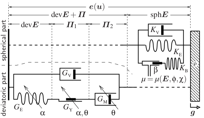
Figure 1: Schematic diagram for the viscoelastic Jeffreys rheology which is subjected to damage $\alpha$ and depending on temperature in the deviatoric part while the Kelvin-Voigt poro-visco-elastic rheology in the spherical (volumetric) part with $\mu$ a pore pressure from (12).

The philosophy of the anisothermal enhancement of Kelvin-Voigt/Jeffreys viscoplastic model is to allow for, beside the friction model (28) below, a mechanically enhanced Stefan-type phase transformation a’la ice-water transformation, as devised in [69]. More specifically, when $G_{\text{\sc m}}=0$, the elastic shear response is completely suppressed and the medium becomes viscoelastic fluid. This situation makes the deviatoric elastic stress ${\rm dev}\bm{S}_{\text{\sc e}}$ zero (so that ${\rm dev}{\bm{E}}=0$) and ${\bm{\varPi}}_{2}$ freely evolving, which causes $\mathchoice{{\buildrel\hskip 1.00006pt{{}_{\,\bm{\circ}}}\over{{\bm{\varPi}}}}}{{\buildrel\hskip 1.00006pt{{}_{\,\bm{\circ}}}\over{{\bm{\varPi}}}}}{{\buildrel\hskip 1.00006pt{\bm{\circ}}\over{{\bm{\varPi}}}}}{{\buildrel\hskip 1.00006pt{\bm{\circ}}\over{{\bm{\varPi}}}}}_{2}={\bm{e}}({\bm{v}})$ so that ${\bm{\varPi}}_{2}={\bm{e}}({\bm{u}})-{\bm{\varPi}}_{1}$. The Jeffreys solid rheology in the deviatoric response then degenerates in the Stokes fluid, while the spherical response remains as the Kelvin-Voigt solid, composing thus a viscoelastic fluid (modelling magma, cf. Section 6 below). This allows for propagation of longitudinal waves in fluidic regions while shear waves are suppressed (or transformed and reflected on the boundaries). Importantly, ${\rm dev}{\bm{E}}=0$ means that ${\bm{E}}=p{\mathbb{I}}/K_{\text{\sc e}}$ for some hydrostatic pressure and (7c) reduces to $\mathchoice{{\buildrel\hskip 1.00006pt\text{\Large\bf.}\over{p}}}{{\buildrel\hskip 1.00006pt\text{\Large\bf.}\over{p}}}{{\buildrel\hskip 1.00006pt\text{\Large.}\over{p}}}{{\buildrel\hskip 1.00006pt\text{\large.}\over{p}}}=K_{\text{\sc e}}{\rm div}\,{\bm{v}}$; here one exploits (3). Also, controlling the modulus $G_{\text{\sc m}}$ by temperature then allows to model melting of rocks to magma and, conversely, solidification of magma to solid rocks, cf. Section 6 below for a more detailed discussion. Notably, although the inelastic strain ${\bm{\varPi}}_{2}$ does not influence the responses in the fluidic state, it nevertheless continues evolving with ${\bm{e}}({\bm{v}})$ so that the possible later solidification performs in the actual configuration reflected by evolved ${\bm{\varPi}}={\bm{\varPi}}_{1}{+}{\bm{\varPi}}_{2}$ while the former configuration at the melting time is naturally forgotten. This allows for repeating arbitrarily many times solid-to-fluid or fluid-to-solid transformations.

Let us still note that the vector of scalar internal variables $w$ opens possibilities for expansions or modifications of the presented model. An example is a combination of damage with so-called breakage [40, 41, 43] for solid-granular materials, where again the coupling with damage as in (26) is considered. Moreover, some coefficients in the dissipative part of the model can be easily made dependent more generally on other variables without changing the structure of the resulting equations and the calculations in Section 7 below, i.e. $K_{\text{\sc v}}=K_{\text{\sc v}}({\rm tr}{\bm{E}},w,\chi,\theta)$, $G_{\text{\sc v}}=G_{\text{\sc v}}({\rm tr}{\bm{E}},w,\chi,\theta)$, $G_{\text{\sc m}}=G_{\text{\sc m}}({\rm tr}{\bm{E}},w,\chi,\theta)$, $K=K({\rm tr}{\bm{E}},w,\chi,\theta)$, or $M=M({\rm tr}{\bm{E}},w,\chi,\theta)$. In particular, the dependence of $G_{\text{\sc v}}$ on ${\rm tr}{\bm{E}}$ (i.e. on the pressure $K_{\text{\sc e}}{\rm tr}{\bm{E}}$) and on $\chi$ allows for making the temperature of the solid-fluid transformation pressure and water-content dependent, which is indeed an important phenomenon in Earth mantle.

5 Tectonic earthquake modelling

In contrast to engineering fracture models, geophysical fast fracture is to be followed by slow healing (also called aging). This prepares a condition for another fracture and thus, considering application to tectonic faults, for re-occurring earthquakes. It seems to bring special demands on successful computation simulations to avoid tendency for aseismic slip instead of a desired stick and healing after each rupture. There exist two possibilities in literature, either to impose some instability by making the stored energy nonconvex in terms of ${\bm{E}}$ when the rock is enough damaged or to impose some slip velocity weakening (modelled here as some yield stress $G_{\text{\sc y}}$ weakening).

As to the first option, an ansatz which is 2-homogeneous in terms of ${\bm{E}}$, suggested in [47], modifies (10) as

$$\varphi({\bm{E}},w,\chi)=\frac{3}{2}K_{\text{\sc e}}(\alpha)|{\rm sph}{\bm{E}}|^{2}\!+G_{\text{\sc e}}(\alpha)|{\rm dev}{\bm{E}}|^{2}\!$$

$$\qquad\qquad\quad-N_{\text{\sc e}}(\alpha){\rm tr}{\bm{E}}\,|{\bm{E}}|+\frac{1}{2\kappa}G_{\text{\sc h}}\alpha^{2}$$

$$\qquad\qquad\qquad\qquad+\frac{3}{2}K_{\text{\sc b}}\Big{|}{\rm sph}{\bm{E}}-\frac{\chi{-}\phi}{3\beta}{\mathbb{I}}\Big{|}^{2}$$ (27)

with some non-Hookean modulus $N_{\text{\sc e}}$ as an increasing function of damage $\alpha$ which, for $\alpha\to 0$, becomes sufficiently large to make $\varphi(\cdot,w,\chi)$ nonconvex. This model was used in a series of articles, cf. e.g. [7, 23, 30, 31, 42, 43, 45, 46, 41] and references therein.

The second option uses (as some departure point) the rate-and-state-dependent Dieterich-Ruina friction model, devised originally in an isothermal variant as a frictional contact problem with some slip velocity weakening of the friction coefficient (called also a sliding resistance) in [19, 77]. This original model seems however incompatible with the 2nd law of thermodynamics (i.e. the entropy Clausius-Duhem inequality), as articulated in [63, Sect. 2]. Yet, a similar instability effect can be obtain by replacing velocity by temperature while relying on that local temperature variation is well related with slip rate during fast earthquakes. This reflects the phenomenon that temperature can locally rise by many hundreds degrees. Such intense heat production during strong earthquakes is referred to as a flash heating, cf. [4, 12, 13, 58, 60]. “Translating” the contact model to the bulk model as suggested in [63, Sect. 6.3] can be performed by making the yield stress $G_{\text{\sc y}}$ dependent on damage (aging) and temperature as

$$G_{\text{\sc y}}(\alpha,\theta)=G_{\text{\sc y0}}+a\Big{(}{\rm ln}\frac{\theta}{v_{\rm ref}\!}+1\Big{)}+b\Big{(}{\rm ln}\frac{\!v_{\rm ref}\alpha\!}{d_{\rm c}}+1\Big{)}\$$ (28)

with (given) parameters $a$ and $b$ (called respectively the direct-effect and evolution friction parameters), $d_{\rm c}$ a characteristic slip memory length, and $v_{\rm ref}$ a reference velocity. The desired velocity weakening occurs if $a<b$.

A simplified friction model with only one parameter is sometimes also considered under the name rate-dependent friction [19, 42, 77, 86] and was analyzed in [48] as far as its stability.

Actually, earthquakes on faults in hydrated rocks can be influenced by the water content by causing additional weakening especially under remarkable flash heating, cf. e.g. [14, 39, 59] or Sect. 3.1 in [55]. This phenomenon can be reflected in our model directly by making $G_{\text{\sc y}}$ dependent also on the water content $\chi$.

6 Rock–magma transition modelling

The ability of the model to cover solid-liquid phase transformation mentioned already in Section  4 can be exploited to model melting / solidification within transformation between solid rocks and fluidic magma. The specific feature is that magma is not exactly a liquid (in particular not an ideal Stokes fluid), being reported as a partially melted rock where shear waves can still propagate although with a reduced velocity [79].

Another feature is that the melting / solidification does not occur at a single melting temperature (in contrast e.g. to a single-component ice-water phase transition) because rocks contain many constituents with different melting temperatures [79]. In particular, the multi-component rock-magma transition is rather “fuzzy” in some temperature interval and, instead of a sharp interface, a mush zone is expected. This can easily be reflected by considering $\gamma$ in (7g) continuous (only with a bigger slope in melting temperature interval).

When melting is completed, $G_{\text{\sc m}}$ in (15) “nearly” (but not completely) vanishes. Although $G_{\text{\sc m}}$ remains non-zero in magma, typical values $10^{4\pm 3}$ Pa s are by many orders lower that in rocks where $G_{\text{\sc m}}$ is about $10^{21\pm 3}$Pa s, as already mentioned. Thus, from longer time scales, magma is not far from being quite ideal fluid.

Simultaneously, when making $[\zeta_{3}]_{w}^{\prime}(w,\theta;\cdot)$ vanishing for $\theta$ above melting temperature, both the damage $\alpha$ and porosity $\phi$ fall fast to zero after the compressed rock is melted to compressed liquid magma.

There are other phenomena [79] which can be incorporated in the model. Specifically, viscosity of magmas slightly decreases with increasing pressure, which suggests to make $G_{\text{\sc m}}$ dependent also on ${\rm tr}{\bm{E}}$, and decreases with the shear rate, i.e. magma is rather a non-Newtonian viscoelastic fluid. This suggests to use (14) with the exponent $p<2$ instead of 2. The latter variant is called a shear thinning. Other phenomenon in the rock-magma system which can be potentially covered by this model is volcanic earthquakes arising from shear fracture in rocks adjacent to magma chambers.

A general phenomenon of buoyancy in the whole mantle [80] is particularly articulated in volcanism because magma is lighter than rocks especially below Mohorovičič discontinuity [79]. Buoyancy is then an important phenomenon which drives movement of magma in mantle and eventually may lead to volcanic activity on the Earth surface. The buoyancy effects can be naturally modelled by thermal expansion of the material. In particular, above melting temperature the material substantially expands and decreases the density $\varrho$, which then decreases the force $\varrho{\bm{g}}$ on the right-hand side of (7b) and thus lead to the buoyancy effect. The term $\frac{3}{2}K_{\text{\sc e}}|{\rm sph}{\bm{E}}|^{2}$ in (10) is to be replaced by $\frac{3}{2}K_{\text{\sc e}}|{\rm sph}{\bm{E}}-\varepsilon(\theta)\mathbb{I}|^{2}$ with some function $\varepsilon(\cdot)$ which increases in particular when temperature $\theta$ passes through the interval of melting temperatures. In other words, the free energy (4) augments by a mixed term $-3K_{\text{\sc e}}\varepsilon(\theta){\rm tr}{\bm{E}}$ while the function $h(\cdot)$ in (4) contains now also $\frac{1}{2}K_{\text{\sc e}}\varepsilon^{2}(\cdot)$, i.e. now

$$\psi({\bm{E}},w,\chi,\nabla w,\theta) =\varphi({\bm{E}},w,\chi)+\frac{\kappa}{2}|\nabla w|^{2}$$

$$\ \ \ \ +h(\theta)-3K_{\text{\sc e}}\varepsilon(\theta){\rm tr}{\bm{E}}\,.$$ (29)

The elastic stress ${\bm{S}}_{\text{\sc e}}$ in (11) then augments by a pressure stress $-3K_{\text{\sc e}}\varepsilon(\theta)\mathbb{I}$ while the heat-transfer equation (7g) augments by an adiabatic heat source/sink $3\theta K_{\text{\sc e}}\varepsilon^{\prime}(\theta){\rm tr}\mathchoice{{\buildrel\hskip 1.00006pt\text{\Large\bf.}\over{{\bm{E}}}}}{{\buildrel\hskip 1.00006pt\text{\Large\bf.}\over{{\bm{E}}}}}{{\buildrel\hskip 1.00006pt\text{\Large.}\over{{\bm{E}}}}}{{\buildrel\hskip 1.00006pt\text{\large.}\over{{\bm{E}}}}}$ and uses $\gamma=\gamma({\bm{E}},\theta)$ depending now also on ${\rm sph}{\bm{E}}$ as

$$\gamma({\bm{E}},\theta)=h(\theta)-\theta h^{\prime}(\theta)-3K_{\text{\sc e}}\big{(}\varepsilon(\theta){-}\theta\varepsilon^{\prime}(\theta)\big{)}{\rm tr}{\bm{E}}\,;$$ (30)

here we assume, without loss of generality, that $\varepsilon(0)=0$, cf. [38, Remark 8.1.4]. Thus the heat capacity is now $c({\rm tr}{\bm{E}},\theta)=-\theta(h^{\prime\prime}(\theta){-}3K_{\text{\sc e}}\varepsilon^{\prime\prime}(\theta){\rm tr}{\bm{E}})$ and, in general, depends also on the pressure through ${\rm tr}{\bm{E}}$ unless $\varepsilon(\cdot)$ is affine.

Yet, it should be said that there are some other mechanisms which may contribute to magma generation than mere increase of temperature.

7 Thermodynamics of the model (7)

Let us derive the energetics behind the system (7). To this goal, we must consider some domain, let us denote it by $\Omega\subset{\mathbb{R}}^{3}$, and its boundary $\Gamma$, and to consider some boundary conditions. For simplicity, let us consider

$$\!\!\!\!{\bm{v}}{\cdot}{\bm{n}}=0,\ \,\big{[}\big{(}\bm{S}_{\text{\sc e}}{+}{\bm{S}}_{\text{\sc v}}{+}{\bm{S}}_{\rm str}\big{)}{\bm{n}}\big{]}_{\text{\sc t}}={\bm{t}},\ \,({\bm{n}}{\cdot}\nabla){\bm{\varPi}}=0,$$ (31a)

$$\!\!\!\!({\bm{n}}{\cdot}\nabla)w=0,\ \ \ \ {\bm{n}}{\cdot}\nabla\mu=0,\ \ \ \ {\bm{n}}{\cdot}K\nabla\theta=j_{\rm ext}$$ (31b)

with ${\bm{n}}$ denoting the outward unit normal to $\Gamma$, $[\cdot]_{\text{\sc t}}$ the tangential component of a vector on $\Gamma$, and ${\bm{t}}$ a traction force and $j_{\rm ext}$ an external heat flux through $\Gamma$.

Multiplying the continuity equation (7a) by $|{\bm{v}}|^{2}/2$, we obtain

$$\frac{\partial{}}{\partial t}\Big{(}\frac{\rho}{2}|{\bm{v}}|^{2}\Big{)} =\rho{\bm{v}}{\cdot}\frac{\partial{{\bm{v}}}}{\partial t}+\frac{\partial{\rho}}{\partial t}\frac{|{\bm{v}}|^{2}}{2}$$

$$=\rho{\bm{v}}{\cdot}\frac{\partial{{\bm{v}}}}{\partial t}-({\bm{v}}{\cdot}\nabla\rho)\frac{|{\bm{v}}|^{2}}{2}-\rho({\rm div}\,{\bm{v}})\frac{|{\bm{v}}|^{2}}{2}\,.$$ (32)

The momentum equation (7b) should be multiplied by the velocity ${\bm{v}}$. The convective term $\varrho({\bm{v}}{\cdot}\nabla){\bm{v}}{\cdot}{\bm{v}}$ contained in $\varrho\mathchoice{{\buildrel\hskip 1.00006pt\text{\Large\bf.}\over{{\bm{v}}}}}{{\buildrel\hskip 1.00006pt\text{\Large\bf.}\over{{\bm{v}}}}}{{\buildrel\hskip 1.00006pt\text{\Large.}\over{{\bm{v}}}}}{{\buildrel\hskip 1.00006pt\text{\large.}\over{{\bm{v}}}}}{\cdot}{\bm{v}}$ gives, when integrated over $\Omega$ and processed by Green’s formula, that

$$\int_{\Omega}\rho({\bm{v}}{\cdot}\nabla){\bm{v}}{\cdot}{\bm{v}}\,{\rm d}x=-\int_{\Omega}{\bm{v}}{\cdot}{\rm div}(\rho{\bm{v}}{\otimes}{\bm{v}})\,{\rm d}x$$

$$\ =-\int_{\Omega}({\bm{v}}{\cdot}\nabla\rho)|{\bm{v}}|^{2}+\rho({\bm{v}}{\cdot}\nabla){\bm{v}}{\cdot}{\bm{v}}+\rho({\rm div}\,{\bm{v}})|{\bm{v}}|^{2}\,{\rm d}x$$

$$\qquad\qquad=-\int_{\Omega}({\bm{v}}{\cdot}\nabla\rho)\frac{|{\bm{v}}|^{2}}{2}+\rho({\rm div}\,{\bm{v}})\frac{|{\bm{v}}|^{2}}{2}\,{\rm d}x$$

$$\qquad\qquad\qquad\quad=\frac{{\rm d}}{{\rm d}t}\int_{\Omega}\frac{\rho}{2}|{\bm{v}}|^{2}\,{\rm d}x-\int_{\Omega}\rho\frac{\partial{{\bm{v}}}}{\partial t}{\cdot}{\bm{v}}\,{\rm d}x\,.$$ (33)

The flow rule (7d) for ${\bm{\varPi}}$ is to be multiplied by $\mathchoice{{\buildrel\hskip 1.00006pt{{}_{\,\bm{\circ}}}\over{{\bm{\varPi}}}}}{{\buildrel\hskip 1.00006pt{{}_{\,\bm{\circ}}}\over{{\bm{\varPi}}}}}{{\buildrel\hskip 1.00006pt{\bm{\circ}}\over{{\bm{\varPi}}}}}{{\buildrel\hskip 1.00006pt{\bm{\circ}}\over{{\bm{\varPi}}}}}$. Using (7c) and the matrix algebra $A{:}(BC)=(B^{\top}\!A){:}C=(AC^{\top}){:}B$, from the term ${\rm dev}\bm{S}_{\text{\sc e}}$ we obtain

$${\rm dev}\bm{S}_{\text{\sc e}}{:}\mathchoice{{\buildrel\hskip 1.00006pt{{}_{\,\bm{\circ}}}\over{{\bm{\varPi}}}}}{{\buildrel\hskip 1.00006pt{{}_{\,\bm{\circ}}}\over{{\bm{\varPi}}}}}{{\buildrel\hskip 1.00006pt{\bm{\circ}}\over{{\bm{\varPi}}}}}{{\buildrel\hskip 1.00006pt{\bm{\circ}}\over{{\bm{\varPi}}}}}=\bm{S}_{\text{\sc e}}{:}\mathchoice{{\buildrel\hskip 1.00006pt{{}_{\,\bm{\circ}}}\over{{\bm{\varPi}}}}}{{\buildrel\hskip 1.00006pt{{}_{\,\bm{\circ}}}\over{{\bm{\varPi}}}}}{{\buildrel\hskip 1.00006pt{\bm{\circ}}\over{{\bm{\varPi}}}}}{{\buildrel\hskip 1.00006pt{\bm{\circ}}\over{{\bm{\varPi}}}}}=\bm{S}_{\text{\sc e}}{:}{\bm{e}}({\bm{v}})-\bm{S}_{\text{\sc e}}{:}\mathchoice{{\buildrel\hskip 1.00006pt{{}_{\,\bm{\circ}}}\over{{\bm{E}}}}}{{\buildrel\hskip 1.00006pt{{}_{\,\bm{\circ}}}\over{{\bm{E}}}}}{{\buildrel\hskip 1.00006pt{\bm{\circ}}\over{{\bm{E}}}}}{{\buildrel\hskip 1.00006pt{\bm{\circ}}\over{{\bm{E}}}}}$$

$$\qquad=\bm{S}_{\text{\sc e}}{:}{\bm{e}}({\bm{v}})-\varphi_{\bm{E}}^{\prime}({\bm{E}},w,\chi){:}\Big{(}\frac{\partial{{\bm{E}}}}{\partial t}+({\bm{v}}{\cdot}\nabla){\bm{E}}\Big{)}$$

$$\qquad\qquad-\bm{S}_{\text{\sc e}}{:}\big{(}{\bm{E}}\,{\rm skew}(\nabla{\bm{v}})-{\rm skew}(\nabla{\bm{v}}){\bm{E}}\big{)}$$

$$\qquad=\Big{(}\bm{S}_{\text{\sc e}}+{\rm skew}\big{(}\bm{S}_{\text{\sc e}}{\bm{E}}^{\top}\!\!-\bm{S}_{\text{\sc e}}^{\top}{\bm{E}}\big{)}\Big{)}{:}{\bm{e}}({\bm{v}})$$

$$\qquad\qquad-\varphi_{\bm{E}}^{\prime}({\bm{E}},w,\chi){:}\Big{(}\frac{\partial{{\bm{E}}}}{\partial t}+({\bm{v}}{\cdot}\nabla){\bm{E}}\Big{)}$$

$$\qquad=\bm{S}_{\text{\sc e}}{:}{\bm{e}}({\bm{v}})-\varphi_{\bm{E}}^{\prime}({\bm{E}},w,\chi){:}\Big{(}\frac{\partial{{\bm{E}}}}{\partial t}+({\bm{v}}{\cdot}\nabla){\bm{E}}\Big{)}\,.$$ (34)

Let us note that actually $\bm{S}_{\text{\sc e}}{\bm{E}}^{\top}\!\!-\bm{S}_{\text{\sc e}}^{\top}{\bm{E}}=0$ because the transport by corotational derivatives keeps elastic strain and stress tensors symmetric, and thus the stress in (7b) is symmetric. This is consistent with the expected symmetry of the Cauchy stress except when also some dipoles (as magnetization or polarization) were transported, cf. [70].

The flow rule (7e) for $w$ is to be multiplied by $\mathchoice{{\buildrel\hskip 1.00006pt\text{\Large\bf.}\over{w}}}{{\buildrel\hskip 1.00006pt\text{\Large\bf.}\over{w}}}{{\buildrel\hskip 1.00006pt\text{\Large.}\over{w}}}{{\buildrel\hskip 1.00006pt\text{\large.}\over{w}}}$, which gives rise in particular to the term

$$\varphi_{w}^{\prime}({\bm{E}},w,\chi)\mathchoice{{\buildrel\hskip 1.00006pt\text{\Large\bf.}\over{w}}}{{\buildrel\hskip 1.00006pt\text{\Large\bf.}\over{w}}}{{\buildrel\hskip 1.00006pt\text{\Large.}\over{w}}}{{\buildrel\hskip 1.00006pt\text{\large.}\over{w}}} =\varphi_{w}^{\prime}({\bm{E}},w,\chi)\frac{\partial{w}}{\partial t}+\varphi_{w}^{\prime}({\bm{E}},w,\chi)({\bm{v}}{\cdot}\nabla)w\,.$$ (35)

Moreover, the gradient term in (7e) can be handled by the calculus together with the Green formula over $\Omega$ as

$$\!\!\!\!\!\!\int_{\Omega}\kappa\Delta w{\cdot}\mathchoice{{\buildrel\hskip 1.00006pt\text{\Large\bf.}\over{w}}}{{\buildrel\hskip 1.00006pt\text{\Large\bf.}\over{w}}}{{\buildrel\hskip 1.00006pt\text{\Large.}\over{w}}}{{\buildrel\hskip 1.00006pt\text{\large.}\over{w}}}\,{\rm d}x=\int_{\Omega}\kappa\Delta w{\cdot}({\bm{v}}{\cdot}\nabla)w\,{\rm d}x-\frac{{\rm d}}{{\rm d}t}\int_{\Omega}\frac{\kappa}{2}|\nabla w|^{2}\,{\rm d}x$$

$$=\int_{\Gamma}\kappa({\bm{n}}{\cdot}\nabla)w{\cdot}({\bm{v}}{\cdot}\nabla)w\,{\rm d}S-\frac{{\rm d}}{{\rm d}t}\int_{\Omega}\frac{\kappa}{2}|\nabla w|^{2}\,{\rm d}x$$

$$\hskip 30.00005pt-\int_{\Omega}\Big{(}\kappa(\nabla w{\otimes}\nabla w){:}{\bm{e}}({\bm{v}})-\frac{\kappa}{2}|\nabla w|^{2}{\rm div}\,{\bm{v}}\Big{)}\,{\rm d}x$$

$$=\int_{\Omega}\Big{(}\frac{\kappa}{2}|\nabla w|^{2}{\mathbb{I}}-\kappa(\nabla w{\otimes}\nabla w)\Big{)}{:}{\bm{e}}({\bm{v}})\,{\rm d}x$$

$$\hskip 120.00018pt-\frac{{\rm d}}{{\rm d}t}\int_{\Omega}\frac{\kappa}{2}|\nabla w|^{2}\,{\rm d}x\,.$$ (36)

We used the boundary condition $({\bm{n}}{\cdot}\nabla)w=0$. Here we can identify the Korteweg-like contribution $\frac{\kappa}{2}|\nabla w|^{2}{\mathbb{I}}-\kappa(\nabla w{\otimes}\nabla w)$ in the structural stress $\bm{S}_{\rm str}$ in (7b).

The product of the two equations in (7f) gives

$$\varphi_{\chi}^{\prime}({\bm{E}},w,\chi)\frac{\partial{\chi}}{\partial t}+D\mathchoice{{\buildrel\hskip 1.00006pt\text{\Large\bf.}\over{\chi}}}{{\buildrel\hskip 1.00006pt\text{\Large\bf.}\over{\chi}}}{{\buildrel\hskip 1.00006pt\text{\Large.}\over{\chi}}}{{\buildrel\hskip 1.00006pt\text{\large.}\over{\chi}}}^{2} =\mu\>{\rm div}(M\nabla\mu)-\varphi_{\chi}^{\prime}({\bm{E}},w,\chi){\bm{v}}{\cdot}\nabla\chi.$$ (37)

Integrating $\mu\>{\rm div}(M\nabla\mu)$ over $\Omega$ and using Green’s formula gives the dissipation rate due to diffusion $\int_{\Omega}M|\nabla\mu|^{2}\,{\rm d}x$.

Summing the partial time-derivative terms in (34), (35), and (37), we can use the calculus

$$\varphi_{\bm{E}}^{\prime}({\bm{E}},w,\chi){:}\frac{\partial{{\bm{E}}}}{\partial t}+\varphi_{w}^{\prime}({\bm{E}},w,\chi){\cdot}\frac{\partial{w}}{\partial t}$$

$$\qquad\qquad\qquad\quad+\varphi_{\chi}^{\prime}({\bm{E}},w,\chi)\frac{\partial{\chi}}{\partial t}=\frac{\partial{}}{\partial t}\varphi({\bm{E}},w,\chi)$$ (38)

to see the main part of the stored energy rate, cf. (60) and (86) below. Furthermore, summing the convective terms in (34), (35), and (37) and using the Green formula when integrating them over $\Omega$, we obtain

$$\int_{\Omega}\Big{(}\varphi_{\bm{E}}^{\prime}({\bm{E}},w,\chi){:}({\bm{v}}{\cdot}\nabla){\bm{E}}$$

$$\qquad+\varphi_{w}^{\prime}({\bm{E}},w,\chi)({\bm{v}}{\cdot}\nabla)w+\varphi_{\chi}^{\prime}({\bm{E}},w,\chi){\bm{v}}{\cdot}\nabla\chi\Big{)}\,{\rm d}x$$

$$=\int_{\Omega}\nabla\varphi({\bm{E}},w,\chi){\cdot}{\bm{v}}\,{\rm d}x$$

$$=\int_{\Gamma}\varphi({\bm{E}},w,\chi){\bm{v}}{\cdot}{\bm{n}}\,{\rm d}S-\int_{\Omega}\varphi({\bm{E}},w,\chi){\rm div}\,{\bm{v}}\,{\rm d}x$$

$$=-\int_{\Omega}\varphi({\bm{E}},w,\chi){\mathbb{I}}{:}{\bm{e}}({\bm{v}})\,{\rm d}x\,;$$ (39)

here we used the boundary condition ${\bm{v}}{\cdot}{\bm{n}}=0$ from (31a) and obtained one part of the pressure contribution $\varphi({\bm{E}},w,\chi){\mathbb{I}}$ in the structural stress $\bm{S}_{\rm str}$ in (7b).

Altogether, summing the above mentioned tests of (7a,c,d,e) and using the boundary conditions in (31), we can exploit the suitably chosen structural stress $\bm{S}_{\rm str}$ in (7b). We can also see cancellation of the right-hand side in (33) with two last terms in (32) integrated over $\Omega$. Thus we eventually obtain the desired energy balance

$$\frac{{\rm d}}{{\rm d}t}\int_{\varOmega}\!\!\!\!\!\begin{array}[t]{c}\begin{array}[t]{c}\underbrace{\frac{\varrho}{2}|{\bm{v}}|^{2}\!\!}\vspace*{.5em}\end{array}\vspace*{-1em}\\ _{\mbox{\footnotesize\rm kinetic}}\vspace*{-.5em}\\ _{\mbox{\footnotesize\rm$$energy}}\end{array}\!\!\!\!\!\!\!+\!\!\!\!\!\!\!\begin{array}[t]{c}\begin{array}[t]{c}\underbrace{\varphi({\bm{E}},w,\chi)+\frac{\kappa}{2}|\nabla w|^{2}\!\!}\vspace*{.5em}\end{array}\vspace*{-1em}\\ _{\mbox{\footnotesize\rm stored energy}}\end{array}\!\!\!\!{\rm d}x$$ (47)

$$\ \qquad\qquad+\int_{\varOmega}\!\!\!\!\!\!\begin{array}[t]{c}\begin{array}[t]{c}\underbrace{\!\!\xi(w,\theta;{\bm{e}}({\bm{v}}),\mathchoice{{\buildrel\hskip 1.00006pt{{}_{\,\bm{\circ}}}\over{{\bm{\varPi}}}}}{{\buildrel\hskip 1.00006pt{{}_{\,\bm{\circ}}}\over{{\bm{\varPi}}}}}{{\buildrel\hskip 1.00006pt{\bm{\circ}}\over{{\bm{\varPi}}}}}{{\buildrel\hskip 1.00006pt{\bm{\circ}}\over{{\bm{\varPi}}}}},\mathchoice{{\buildrel\hskip 1.00006pt\text{\Large\bf.}\over{w}}}{{\buildrel\hskip 1.00006pt\text{\Large\bf.}\over{w}}}{{\buildrel\hskip 1.00006pt\text{\Large.}\over{w}}}{{\buildrel\hskip 1.00006pt\text{\large.}\over{w}}},\nabla\mu,\mathchoice{{\buildrel\hskip 1.00006pt\text{\Large\bf.}\over{\chi}}}{{\buildrel\hskip 1.00006pt\text{\Large\bf.}\over{\chi}}}{{\buildrel\hskip 1.00006pt\text{\Large.}\over{\chi}}}{{\buildrel\hskip 1.00006pt\text{\large.}\over{\chi}}},\nabla\mathchoice{{\buildrel\hskip 1.00006pt{{}_{\,\bm{\circ}}}\over{{\bm{\varPi}}}}}{{\buildrel\hskip 1.00006pt{{}_{\,\bm{\circ}}}\over{{\bm{\varPi}}}}}{{\buildrel\hskip 1.00006pt{\bm{\circ}}\over{{\bm{\varPi}}}}}{{\buildrel\hskip 1.00006pt{\bm{\circ}}\over{{\bm{\varPi}}}}})\!\!\!}\vspace*{.5em}\end{array}\vspace*{-1em}\\ _{\mbox{\footnotesize\rm dissipation rate}}\end{array}\!\!\!\!\!\!{\rm d}x$$ (51)

$$\hskip 10.00002pt=\int_{\varOmega}\!\!\!\!\!\!\!\begin{array}[t]{c}\begin{array}[t]{c}\underbrace{\varrho{\bm{g}}{\cdot}{\bm{v}}-h(\theta){\rm div}\,{\bm{v}}\!\!}\vspace*{.5em}\end{array}\vspace*{-1em}\\ _{\mbox{\footnotesize\rm power of external load}}\vspace*{-.5em}\\ _{\mbox{\footnotesize\rm and of adiabatic effects}}\end{array}\!\!\!\!\!{\rm d}x+\int_{\varGamma}\!\!\!\!\!\!\!\!\!\!\!\!\!\!\begin{array}[t]{c}\begin{array}[t]{c}\underbrace{\,{\bm{t}}{\cdot}{\bm{v}}\!}\vspace*{.5em}\end{array}\vspace*{-1em}\\ _{\mbox{\footnotesize\rm power of}}\vspace*{-.5em}\\ _{\mbox{\footnotesize\rm traction load}}\end{array}\!\!\!\!\!\!\!\!\!\!\!\!\!\!{\rm d}S\,.$$ (60)

Adding (7g) integrated over $\Omega$, the dissipation term $\xi$ and the adiabatic terms on the right-hand side of (7g) cancel. Using also the last boundary condition in (31b), we thus obtain the total energy balance

$$\frac{{\rm d}}{{\rm d}t}\int_{\varOmega}\!\!\!\!\!\begin{array}[t]{c}\begin{array}[t]{c}\underbrace{\frac{\varrho}{2}|{\bm{v}}|^{2}\!\!}\vspace*{.5em}\end{array}\vspace*{-1em}\\ _{\mbox{\footnotesize\rm kinetic}}\vspace*{-.5em}\\ _{\mbox{\footnotesize\rm$$energy}}\end{array}\!\!\!\!\!\!+\!\!\!\!\!\!\begin{array}[t]{c}\begin{array}[t]{c}\underbrace{\varphi({\bm{E}},w,\chi)+\frac{\kappa}{2}|\nabla w|^{2}\!\!}\vspace*{.5em}\end{array}\vspace*{-1em}\\ _{\mbox{\footnotesize\rm stored}}\vspace*{-.5em}\\ _{\mbox{\footnotesize\rm$$energy}}\end{array}\!\!\!\!+\!\!\!\!\!\!\!\!\!\!\!\!\!\!\!\!\!\!\!\!\!\!\!\begin{array}[t]{c}\begin{array}[t]{c}\underbrace{\vartheta\!\!}\vspace*{.5em}\end{array}\vspace*{-1em}\\ _{\mbox{\footnotesize\rm internal heat}}\vspace*{-.5em}\\ _{\mbox{\footnotesize\rm$$energy (enthalpy)}}\end{array}\!\!\!\!\!\!\!\!\!\!\!\!\!\!\!\!\!\!\!\!\!\,{\rm d}x$$ (73)

$$\ \ =\ \ \int_{\varOmega}\!\!\!\!\!\!\!\!\!\!\!\!\!\!\!\!\!\!\!\begin{array}[t]{c}\begin{array}[t]{c}\underbrace{\varrho{\bm{g}}{\cdot}{\bm{v}}\!\!\!}\vspace*{.5em}\end{array}\vspace*{-1em}\\ _{\mbox{\footnotesize\rm external mechanical}}\vspace*{-.5em}\\ _{\mbox{\footnotesize\rm$$bulk power}}\end{array}\!\!\!\!\!\!\!\!\!+\!\!\!\!\!\begin{array}[t]{c}\begin{array}[t]{c}\underbrace{\!\!r\!\!}\vspace*{.5em}\end{array}\vspace*{-1em}\\ _{\mbox{\footnotesize\rm bulk}}\vspace*{-.5em}\\ _{\mbox{\footnotesize\rm heat power}}\end{array}\!\!\!\!\!\!\!\!\!{\rm d}x+\int_{\varGamma}\!\!\!\!\!\!\!\!\!\!\!\!\!\!\!\!\!\!\begin{array}[t]{c}\begin{array}[t]{c}\underbrace{{{\bm{t}}{\cdot}{\bm{v}}+j_{\rm ext}}\!\!\!\!\!\!}\vspace*{.5em}\end{array}\vspace*{-1em}\\ _{\mbox{\footnotesize\rm power of traction and }}\vspace*{-.5em}\\ _{\mbox{\footnotesize\rm of external heating}}\end{array}\!\!\!\!\!\!\!\!\!\!\!\!\!{\rm d}S\,.$$ (86)

For the case of a gravitation acceleration ${\bm{g}}=-\nabla u$ with the potential $u$ from (13), we can be more specific as far as the external load in (60) and (86) concerns. Then the bulk force $\varrho{\bm{g}}$ in the momentum equation tested by ${\bm{v}}$ together with (13) tested by $\frac{\partial{}}{\partial t}u$ results to

$$\int_{\Omega}\!\!-\varrho\nabla u{\cdot}{\bm{v}}\,{\rm d}x=\int_{\Omega}{\rm div}(\varrho{\bm{v}})u\,{\rm d}x$$

$$\quad=-\int_{\Omega}\frac{\partial{\varrho}}{\partial t}u\,{\rm d}x=\int_{\Omega}\varrho\frac{\partial{u}}{\partial t}\,{\rm d}x-\frac{{\rm d}}{{\rm d}t}\int_{\Omega}\varrho u\,{\rm d}x$$

$$\qquad\ =-\frac{{\rm d}}{{\rm d}t}\Big{(}\int_{{\mathbb{R}}^{3}}\frac{1}{2\text{\large$\mathfrak{g}$}}|\nabla u|^{2}\,{\rm d}x+\int_{\Omega}\varrho u\,{\rm d}x\Big{)}\,,$$ (87)

where we used also the continuity equation (7a) and the boundary condition ${\bm{v}}{\cdot}{\bm{n}}=0$. It reveals the energy of the gravitation field and the energy of the mass $\varrho$ in this (self-induced) gravitation field. The energy identities (60) and (86) can then be specified accordingly. In particular, if the system is isolated in the sense ${\bm{t}}={\bm{0}}$ and $j_{\rm ext}=0$, then (86) gives the total energy conservation

$$\int_{\varOmega}\frac{\varrho}{2}|{\bm{v}}|^{2}+\varphi({\bm{E}},w,\chi)+\frac{\kappa}{2}|\nabla w|^{2}+\vartheta+\varrho u\,{\rm d}x\ \$$

$$+\int_{{\mathbb{R}}^{3}}\frac{1}{2\text{\large$\mathfrak{g}$}}|\nabla u|^{2}\,{\rm d}x={\rm const.}$$ (88)

An important attribute of the model, beside keeping the energetics (60)–(86), is the entropy imbalance, i.e. the Clausius-Duhem inequality. The specific entropy $\eta=-\psi_{\theta}^{\prime}=-h^{\prime}(\theta)$ as an extensive variable (in JK^-1m^-3) and its transport and production is governed by the entropy equation:

$$\frac{\partial{\eta}}{\partial t}+{\rm div}({\bm{v}}\,\eta)=\frac{\xi-{\rm div}\,{\bm{j}}+r}{\theta}$$ (89)

with $\xi$ denoting the heat production rate by mechanical/diffusion dissipative processes, cf. (6), and ${\bm{j}}$ the heat flux which is here governed by the Fourier law ${\bm{j}}=-K\nabla\theta$, cf. (7g). The ultimate assumptions $\xi+r\geq 0$ and $K$ positive then ensure the entropy imbalance

$$\frac{{\rm d}}{{\rm d}t}\int_{\Omega}\eta\,{\rm d}x\geq\int_{\Gamma}\!\!\!\!\!\begin{array}[t]{c}\begin{array}[t]{c}\underbrace{({\bm{v}}\eta-{\bm{j}}/\theta)}\vspace*{.5em}\end{array}\vspace*{-1em}\\ _{\mbox{\footnotesize\rm entropy flux}}\end{array}\!\!\!\!\!\!\!\cdot{\bm{n}}\,{\rm d}S=\int_{\Gamma}\frac{j_{\rm ext}}{\theta}\,{\rm d}S$$ (93)

by the usual calculus using also the boundary conditions (31), relying on positivity of temperature. Substituting $\eta=-h^{\prime}(\theta)$ into (89), we obtain the heat-transfer equation

$$c(\theta)\mathchoice{{\buildrel\hskip 1.00006pt\text{\Large\bf.}\over{\theta}}}{{\buildrel\hskip 1.00006pt\text{\Large\bf.}\over{\theta}}}{{\buildrel\hskip 1.00006pt\text{\Large.}\over{\theta}}}{{\buildrel\hskip 1.00006pt\text{\large.}\over{\theta}}}=\xi-{\rm div}\,{\bm{j}}-\vartheta\eta\,{\rm div}\,{\bm{v}}+r$$

$$\qquad\text{ with the heat capacity }\ c(\theta)=-\theta h^{\prime\prime}(\theta)\,;$$ (94)

note that temperature (in K) is an intensive variable and is thus transported by the material derivative while the adiabatic heat term $\theta\eta\,{\rm div}\,{\bm{v}}$ occurs on the right-hand side due to the compressibility of the material. Furthermore, the internal energy is given by the Gibbs relation $\psi+\theta\eta$. In view of (4), it splits here into the purely mechanical part $\varphi({\bm{E}},w,\chi)+\frac{\kappa}{2}|\nabla w|^{2}$ and the thermal part $\vartheta=h(\theta)-\theta h^{\prime}(\theta)=:\gamma(\theta)$. The thermal internal energy $\vartheta$ in Jm^-3 is again an extensive variable and is transported like (89), resulting here to the equation

$$\frac{\partial{\vartheta}}{\partial t}+{\rm div}\big{(}{\bm{v}}\,\vartheta\big{)}=\xi-{\rm div}\,{\bm{j}}+h(\theta){\rm div}\,{\bm{v}}+r\,,$$ (95)

which reveals the structure of (7g).

For (93), we actually needed that $\theta$ is positive, i.e. the model complies with the Nernst 3rd law of thermodynamics. This is really guaranteed in the model (7) under some natural assumptions, namely that $\gamma$ is increasing function of temperature with $\gamma(0)=0$, and $h$ in (4) is concave with $h(0)=0$. Then $\theta\geq 0$ provided the initial temperature is non-negative and provided the boundary heat flux $j_{\rm ext}$ in (31b) is non-negative or, more generally, $j_{\rm ext}$ is a continuous function of temperature and is non-negative for $\theta=0$.

For the generalization (29), the entropy depends on ${\rm tr}{\bm{E}}$ as $\eta=\eta({\rm tr}{\bm{E}},\theta)=3K_{\text{\sc e}}\varepsilon^{\prime}(\theta){\rm tr}{\bm{E}}-h^{\prime}(\theta)$. The right-hand side of the mechanical energy balance (60) then expands by the adiabatic term $-3K_{\text{\sc e}}\varepsilon(\theta){\rm div}\,{\bm{v}}$ while (86) uses $\vartheta=\gamma({\bm{E}},\theta)$ from (30).

8 A semi-compressible variant

The core of the model, i.e. the mass and momentum conservation (7a,b), is “borrowed” from fully compressible fluids covering also gases. Most solid and liquid materials (and in particular rocks and magmas) are not much compressible, however. In particular, density variations are not much pronounced. In a lot of studies, e.g. [30, 43, 45, 46, 90], the mass density $\varrho$ is simply considered constant. This would be well eligible in incompressible models in media which are spatially homogeneous as far as mass density $\varrho$ concerns. Yet, incompressible models do not facilitate propagation of longitudinal seismic waves, which would be an essential drawback of such models in geophysical context. For this reasons, compressible models can be considered in a simplified, compromising, so-called semi-compressible [68] variant relying on that rocks and magmas are only slightly compressible so that, assuming also that the particular space-time region of interest in the mantle is relatively small and thus the mass density $\varrho$ does not vary substantially. This is in particular a relevant simplification if pressure variations are negligible comparing to the bulk elastic modulus. In some approximation, $\varrho$ can then be considered constant and the continuity equation (7a) is avoided. Yet, to keep energy conservation, one has to involve a certain structural acceleration ${\bm{g}}_{\rm str}$ into the momentum equation (7b), which then looks as

$$\!\!\!\varrho\mathchoice{{\buildrel\hskip 1.00006pt\text{\Large\bf.}\over{{\bm{v}}}}}{{\buildrel\hskip 1.00006pt\text{\Large\bf.}\over{{\bm{v}}}}}{{\buildrel\hskip 1.00006pt\text{\Large.}\over{{\bm{v}}}}}{{\buildrel\hskip 1.00006pt\text{\large.}\over{{\bm{v}}}}}={\rm div}\big{(}\bm{S}_{\text{\sc e}}+{\bm{S}}_{\text{\sc v}}+{\bm{S}}_{\rm str}\big{)}+\varrho({\bm{g}}+{\bm{g}}_{\rm str})\quad\ \ \$$

$$\text{ with }\ \ {\bm{g}}_{\rm str}=-\,\frac{1}{2}({\rm div}\,{\bm{v}})\,{\bm{v}}\,.$$ (96)

The force $\varrho{\bm{g}}_{\rm str}$ was invented in [83] rather for numerical purposes to approximate an incompressible model, and recently physically analyzed in [85] where it was pointed out that this force does not comply with Galilean invariancy principle. Of course, in only slightly compressible materials, ${\rm div}\,{\bm{v}}$ and also this extra force is only small and the Galilean invariancy is violated only a little, which is an acceptable price for keeping the energetics holding in this simplified model.

The calculus (33) is to be then replaced by

$$\int_{\Omega}\varrho({\bm{v}}{\cdot}\nabla){\bm{v}}{\cdot}{\bm{v}}\,{\rm d}x=-\int_{\Omega}\varrho{\bm{v}}{\cdot}{\rm div}({\bm{v}}{\otimes}{\bm{v}})\,{\rm d}x$$

$$\qquad=-\int_{\Omega}\varrho|{\bm{v}}|^{2}{\rm div}\,{\bm{v}}+\varrho\nabla{\bm{v}}{:}({\bm{v}}{\otimes}{\bm{v}})\,{\rm d}x$$

$$\qquad\quad=-\int_{\Omega}\frac{\varrho}{2}|{\bm{v}}|^{2}{\rm div}\,{\bm{v}}\,{\rm d}x=\int_{\Omega}{\bm{g}}_{\rm str}{\cdot}{\bm{v}}\,{\rm d}x\,,$$ (97)

where the boundary condition ${\bm{n}}{\cdot}{\bm{v}}=0$ and the spatial constancy of $\varrho$ have been exploited. In this way, the energetics (60) and (86) is preserved.

Having $\varrho$ constant, the buoyancy effects must be modelled also in a simplified way by putting $(1{-}b(\theta)){\bm{g}}$ with some increasing function $b(\cdot)$ instead of ${\bm{g}}$ into (7b) and (60). This is referred as Oberbeck-Boussinesq’s approximation. Then the right-hand side of (7g) is to be augmented by the adiabatic heat source/sink $\varrho b(\theta){\bm{g}}{\cdot}{\bm{v}}$. If the buoyancy $b$ equals 0 for $\theta=0$, then $\theta\geq 0$ is again guaranteed.

One of the property of the full model (7) is difficulty of a rigorous mathematical analysis as far as existence of solution of the system (7) with the boundary conditions (31) in some reasonable sense. If performed in a constructive way by some approximation, such a mathematical analysis usually suggests also computational implementable approximation strategies which are numerically stable and convergent. This justifies theoretical studies also of geophysical models, although it is mostly ignored. Unfortunately, such an analysis of the incompressible model (7) seems not available and is likely very nontrivial unless some higher-gradient modifications are adopted.

Various gradient enhancements of the plain semi-compressible model (i.e. without internal variables) has been devised in [68] where also various impacts on dispersion of elastic (seismic) velocities are discussed. The particular enhancement by dissipative gradient terms exploits the general ideas of multipolar (also called non-simple) media in [29] adopted for fluids in [5, 6, 24, 50, 51, 52]. More specifically, we use nonlinear 2nd-grade nonsimple fluids, also called bipolar fluids, which uses the dissipation potential $\zeta_{1}$ expanded as $\zeta_{1}({\bm{e}}({\bm{v}}))+\nu|\nabla{\bm{e}}({\bm{v}})|^{p}/p$ with some coefficient $\nu>0$ and some $p>3$. Then the viscous stress is augmented as ${\bm{S}}_{\text{\sc v}}=\zeta_{1}^{\prime}({\bm{e}}({\bm{v}}))-{\rm div}(\nu|\nabla{\bm{e}}({\bm{v}})|^{p-2}\nabla{\bm{e}}({\bm{v}}))$ and also the dissipation rate $\xi$ now involves an additionally heat source $\nu|\nabla{\bm{e}}({\bm{v}})|^{p}$. Moreover, as (96) would become a 4th-order parabolic equation, the boundary conditions (31a) have to be augmented by one more higher-order condition.

It should be mention as a general observation that the present state of art in applied-science literature is that many continuum-mechanical models likely do not admit any solutions in whatever reasonable generalized sense, although computational simulations of certain approximate variants are successfully launched for special data. Anyhow, having mere existence of solutions and possible convergence of approximate problems is of theoretical interest.

Here, let us only briefly mention that, in the semi-compressible variant, a rigorous mathematical analysis of the system (7c–g) with (96) with ${\bm{S}}_{\text{\sc v}}$ and $\xi$ augmented by the multipolar terms as mentioned above can be performed by merging and modified the results available for an anisothermal model with damage [69] with the isothermal diffusion model [73]. The essential point is to have boundedness of the velocity gradient $\nabla{\bm{v}}(t)$ in space at particular time instants $t$ and sufficiently smooth initial conditions. The variant of a stored energy nonconvex in term of ${\bm{E}}$ like (27) can be analytically handled easily except that certain modification for large $|{\bm{E}}|$ is desirable to avoid nonphysical fall of energy to $-\infty$ if $|{\bm{E}}|\to\infty$.

9 Conclusion

Let us summarize that a mechanically and thermomechanically consistent model was devised with the goal to improve and complete several existing models previously occurring in literature. The main applications are presumably to tectonic and volcanic processes as well as sources of seismic waves and their propagation in the crust and the upper mantle, although it is not limitted to those. The unified description of these processes thus allows for their natural coupling.

The Eulerian formulation, being more natural in the context of absence of any natural reference configuration, also enables for an easy enhancement of the model by interaction of some spatial fields towards global-type models, as gravitational (considered in Sect. 4) or geomagnetical applied to paleomagnetism in rocks. In the latter case, interestingly the transport of the dipole momentum (i.e. the magnetization) leads to a skew-symmetric contribution to the structural stress, cf. [70]. Also coupling with basic models in hydrosphere (with $\chi$ representing salinity of water in oceans) is possible to model interaction with lithosphere during propagation of seismic waves or tsunamis caused by uplifts of sea beds within earthquakes. Actually, the diffusant content $\chi$ can be vector-valued in some applications, specifically if several constituents are moving independently through porous rocks. This can be in particular water and CO₂, as in [53], or water and oil. The “monolithic” description of visco-elastic solid and fluidic areas allows for a simple modelling of seismic waves propagation in such heterogeneous media, leading to reflection and refraction on the solid/fluid interfaces as well as transformation between longitudinal (pressure) waves and shear waves, cf. [75] for a small-strain variant of the model. The melting/solidification and flow/creep modelling can be applied globally on the mantle, i.e. including its deeper parts (astenosphere) and lower mantle with plumes of hot material or with falling cold slabs, not being confined only on the crust and the subcrustal lithosphere. A more general free energy $\psi$ may allow for phase-transition modelling in volumetric part during recrystalization on upper/lower mantle interface. Also nonnegligible superheating/supercolling effects during magma solidification (cf. [32]) can be incorporated into the model – see [69] for one option in this direction.

As far as magma models, there exist two-phase magma dynamics models which consider rocks and magma as a mixture. A simple example is [35] which however is fully incompressible (i.e. no pressure waves can propagate) and no melting or solidification is, in fact, allowed and energy conservation is not ensured. For a compressible or a multi-component variant see [16, 26, 93] or [36], respectively. Other models by [8] or [81] allow for melting/solidification and consider energy conservation in the continuous model but are again incompressible. Balancing momenta of each constituents separately is a rational approach usually credited by [87], working satisfactorily rather for two-component mixtures only, cf. [62], in contrast to a phenomenological Nobel-prize awarded approach by [56]. Cf. [78] for a comparison of these mixture approaches. In comparison, our model is “monolithic”, reflecting the fact that rocks and magma are actually the same material which is only in different mechanical state depending mainly on temperature and pressure, anyhow allowing, in addition, for a possible phenomenological diffusion of some constituents (e.g. water, hydrated minerals, or oil) and in addition for a fracture in the solid regions (which may lead to volcanic earthquakes) and for a pressure wave propagation. In fact, the mentioned diffusion which resulted by the Biot model is a flow due to Fick or Darcy law (cf. Sect. 3.6 in [38]) and represents a simplest variant of the hierarchy of several porous-media models, cf. [61].

An alternative to the semi-compressible simplification from Section 8, where the inertia is kept in the model but mass density variations are neglected both in time and space (i.e. $\varrho$ is constant), can be just opposite: inertia to be neglected by considering zero acceleration $\mathchoice{{\buildrel\hskip 1.00006pt\text{\Large\bf.}\over{{\bm{v}}}}}{{\buildrel\hskip 1.00006pt\text{\Large\bf.}\over{{\bm{v}}}}}{{\buildrel\hskip 1.00006pt\text{\Large.}\over{{\bm{v}}}}}{{\buildrel\hskip 1.00006pt\text{\large.}\over{{\bm{v}}}}}=0$ but mass density $\varrho$ to allow to vary according to some state equation, being a function of pressure and temperature, cf. [26]. Of course, such quasistatic (or sometimes called quasi-dynamical) models suppress not only seismic pressure wave propagation (like in incompressible variants) but also shear waves. On the other hand, they can still cover many medium- and long-time scale phenomena in a computationally efficient way, cf. e.g. [9, 8, 16, 27, 33, 35, 37, 54, 84].

In the quasistatic variant, the buoyancy model of the Oberbeck-Boussinesq type as mentioned in Section 8 has been used e.g. in [16, 33, 37] in a thermodynamically consistent variant including adiabatic effects or also in e.g. in [9, 27, 54, 84] with adiabatic effects neglected. These quasistatic buoyancy models, in fact, consider the mass density temperature dependent.

Eventually, let us conceptually discuss some implementation issues. It has been articulated in [20] that “computational modeling in geology requires numerical methods that are robust, reliable and accurate”. The robustness and reliability should be supported by rigorous mathematical proofs of existence of solutions to the particular models and of data-depending bounds of solutions obtained by specific approximation methods, leading (under some assumptions on the data) to guaranteed numerical stability and convergence of particular discretization methods. Even more demanding numerical analysis might yield estimates of rates of discretization errors, although this is rarely available. For very practical reasons, such theoretical justification is largely ignored in computational (geo)physics as well as in engineering, being substituted by particular computational simulations and comparison with available experiments, which however, strictly speaking, cannot be considered as a really rigorous proof of robustness and reliability. Many models used in geophysics even have no guaranty for mere existence of solutions in any reasonable sense.

At this occasion, it should be mention that, in general, the consistent physically motivated energetics like this one presented here in Sect. 7 opens possibilities

for designing numerically stable and convergent approximation schemes. This can be a nontrivial task in particular models, however. Here, more specifically, the semicompressible variant from Section 8 bears fully implicit time discretization (i.e. the backward Euler method with possible semi-implicitly handled coefficients in dissipative terms), cf. [69] and, for fine numerical aspects of fully implicit time discretization of problems with nonconvex energies, also [67]. Notably, the objective time derivatives in (7c–g) do not allow for staggered time discretization, which in the non-convective variant would be efficient and even energy conserving, cf. [65].

Of course, the fully implicit time and space discretization leads to nonlinear algebraic systems at each time level to be solved only iteratively, which might be algorithmically rather demanding in situation when fast evolving processes (in particular during rupture and earthquakes) would occur. Beside, some adaptive refinements both of time discretization and space discretization would be desired (e.g. fine time discretization is needed only during ongoing ruptures and propagation of seismic waves and, in most situations, damage is localized only around existing faults). The adaptively varying time step is well facilitated by one-step discretization and, except explicit time discretization methods, the stability of the resulted scheme is not corrupted by large time steps. Such algorithmic and implementation issues would be surely very demanding especially in full model and they have been out of scope of this theoretical article, as well as launching some computational simulations even for some partial, simplified variant of this model.

Algorithmically, truly efficient calculations of seismic waves need an explicit time discretisation at least of the elastodynamical part, cf. [74]. Of course, these time discretisations are to be combined with space discretization by some standard methods like finite or spectral elements, although the objective time derivatives again makes the numerical analysis very technical because they do not stay functions in the respective finite-dimensional spaces. The calculations from Section 7 leading to the desired energetics thus could not be executed directly for the spatially discretized problem and would have to be done successively, likely with other regularizing gradient terms. Even more, the explicit time discretizations work successfully for hyperbolic-type problems, which would here require to suppress the dissipative stress ${\bm{S}}_{\text{\sc v}}$ but this would corrupt the theoretical arguments behind existence of solutions of the model mentioned in Section 8. The fully compressible model with the continuity equation (7) would be even more delicate and combination with discretization methods for mere compressible fluids as [18, 21] should be elaborated. Rather, it is expected that only the mentioned quasistatic variant of the model (7) bears really efficient computational implementation.

Acknowledgments.

The author is deeply thankful to Dr. Vladimir Lyakhovsky for inspiring discussions in 2014 during author’s visit of the Geological Survey of Israel, and to two referees for critical reading of the original version and many valuable suggestions. Also the support from the MŠMT ČR (Ministry of Education of the Czech Republic) project CZ.02.1.01/0.0/0.0/15-003/0000493 and the institutional support RVO:61388998 (ČR) are acknowledged.

References

- [1]
- [1] Ambrosio, L. & Tortorelli, V.M., 1992. On the approximation of free discontinuity problems. Bollettino Unione Mat. Italiana, 7:105–123.
- [2] Babeyko, A.Y. & Sobolev, S.V., 2008. High-resolution numerical modeling of stress distribution in visco-elasto-plastic subducting slabs. Lithos, 103:205–216.
- [3] Bedford, A., 1985. Hamilton’s Principle in Continuum Mechanics. Pitman, Boston.
- [4] Beeler, N.M., Tullis, T.E. & Goldsby, D.L. Constitutive relationships and physical basis of fault strength due to flash heating. J. geophys. Res., 113:B01401, 1–12, 2008. doi:10.1029/2007JB004988.
- [5] Bellout, H., Bloom, F. & Nečas. J. Phenomenological behavior of multipolar viscous fluids. Qarterly Appl. Math., 1:559–583, 1992.
- [6] Bellout, H., Nečas, J. & Rajagopal, K.R. On the existence and uniqueness of flows multipolar fluids of grade 3 and their stability. Intl. J. Engineering Sci., 37:75–96, 1999.
- [7] Ben-Zion, Y. Collective behavior of earthquakes and faults: Continuum-discrete transitions, progressive evolutionary changes, and different dynamic regimes. Rev. Geophys., 46:RG4006, doi:10.1029/2008RG000260, 2008.
- [8] Bercovici, D., Ricard, Y. & Schubert, G., 2001. A two-phase model for compaction and damage. 1. General Theory, J. Geophys. Res., 106(B5), 8887–8906.
- [9] Beuchert, M.J. & Podladchikov, Y.Y., 2010. Viscoelastic mantle convection and lithospheric stresses. Geophys. J. Int., 183, 35–63.
- [10] Billen, M.I. & Hirth, G. Rheologic controls on slab dynamics. Geochem. Geophys. Geosystems, 8(8), 2007.
- [11] Biot, M.A. Mechanics of Incremental Deformation. J. Wiley, 1965.
- [12] Bizzarri, A. The mechanics of lubricated faults: Insights from 3-D numerical models. J. Geophys. Res., 117:B05304, 2012.
- [13] Bizzarri, A. & Cocco, M. Slip-weakening behavior during the propagation of dynamic ruptures obeying rate- and state-dependent friction laws. J. Geophys. Res., 108:2373, 2003.
- [14] Chester, F.M. A rheologic model for wet crust applied to strike-slip faults. J. Geophys. Res. 100:B7,13,033–3,044, 1995.
- [15] Dal Zilio, L., van Dinther, Y., Gerya, T.V. & Pranger, C.C. Seismic behaviour of mountain belts controlled by plate convergence rate. Earth Planetary Sci. Letters, 482:81–92, 2018.
- [16] Dannberg. J. & Heister, T. Compressible magma/mantle dynamics: 3-D, adaptive simulations in ASPECT. Geophys. J. Int. 207:1343–1366, 2016.
- [17] Davoli, E., Roubíček, T., & Stefanelli, U. A note about hardening-free viscoelastic models in Maxwellian-type rheologies. (Preprint arXiv no.2012.08914, 2020.) Math. Mech. Solids, in print, DOI: 10.1177/1081286521990418.
- [18] Dolejší, V. & Feistauer, M. Discontinuous Galerkin Method – Analysis and Applications to Compressible Flow. Springer, Cham/Switzerland, 2015.
- [19] Dieterich, J.H. Modelling of rock friction. Part 1: Experimental results and constitutive equations. J. Geophys. Res., 84(B5):2161–2168, 1979.
- [20] Duretz, T., May, D.A., Gerya, T.V. & Tackley, P.J. Discretization errors and free surface stabilization in the finite difference and marker-in-cell method for applied geodynamics: a numerical study. Geochem. Geophys. Geosyst., 12:Q07004, 2011.
- [21] Feireisl, E., Karper, T.G. & Pokorný, M. Mathematical Theory of Compressible Viscous Fluids – Analysis and Numerics. Springer, Cham/Switzerland, 2016.
- [22] Fiala, Z. Geometrical setting of solid mechanics. Annals of Physics, 326:1983–1997, 2011.
- [23] Finzi, Y., Muhlhaus, H., Gross, L. & Amirbekyan, A. Shear band formation in numerical simulations applying a continuum damage rheology model. Pure Appl. Geophys., 170:13–25, 2013.
- [24] Fried E. & Gurtin, M.E. Tractions, balances, and boundary conditions for nonsimple materials with application to liquid flow at small-length scales. Archive Ration. Mech. Anal., 182:513–554, 2006.
- [25] Gabriel, A.-A. et al. A unified first-order hyperbolic model for nonlinear dynamic rupture processes in diffuse fracture zones. Phil. Trans. R. Soc. A 379:20200130, 2021.
- [26] Gerya, T.V. Introduction to Numerial Geodynamic Modelling. 2nd ed. Cambridge Univ. Press, New York, 2019.
- [27] Gerya, T.V. & Yuen, D.A. Robust characteristics method for modelling multiphase visco-elasto-plastic thermo-mechanical problems. Phys. Earth Planetary Interiors, 163:83–105, 2007.
- [28] Godunov, S.K. & Peshkov, I.M. Thermodynamically consistent nonlinear model of elastoplastic Maxwell medium. Comp. Math. Math. Phys., 50:1409–1426, 2010.
- [29] Green A.E. & Rivlin, R.S. Multipolar continuum mechanics. Arch. Rat. Mech. Anal., 17:113–147, 1964.
- [30] Hamiel, H., Lyakhovsky, V. & Agnon, A. Coupled evolution of damage and porosity in poroelastic media: theory and applications to deformation of porous rocks. Geophys. J. Int., 156:701–713, 2004.
- [31] Hamiel, Y., Lyakhovsky, V., Stanchits, S., Dresen, G. & Ben-Zion, Y. Brittle deformation and damage-induced seismic wave anisotropy in rocks. Geophys. J. Int., 178:901–909, 2009.
- [32] Hammer, J.E. Experimental studies of the kinetics and energetics of magma crystallization. Reviews in Mineralogy & Geochemistry, 69:9–59, 2008.
- [33] Herrendörfer, R., Gerya, T. & van Dinther, Y. An invariant rate- and state-dependent friction formulation for viscoeastoplastic earthquake cycle simulations. earthquake cycle simulations. J. Geophys. Res.: Solid Earth, 123:5018–5051, 2018.
- [33] Jacquey, A.B. & Cacace, M. Multiphysics modeling of a brittle-ductile lithosphere: 1. Explicit visco-elasto-plastic formulation and its numerical implementation. J. Geophys. Res.: Solid Earth, 125:1–21, 2020.
- [34] Jaumann, G. Geschlossenes System physikalischer und chemischer Differentialgesetze. Sitzungsber. der kaiserliche Akad. Wiss. Wien (IIa), 120:385–530, 1911.
- [35] Keller T., May D.A. & Kaus B.J.P., 2013. Numerical modelling of magma dynamics coupled to tectonic deformation of lithosphere and crust, Geophys. J. Int., 195, 1406–1442.
- [36] Keller, T. & Suckale, J. A continuum model of multi-phase reactive transport in igneous systems. Geophysical J. Int., 219, 185–222, 2019.
- [37] Kronbichler, M., Heister, T. & Bangerth, W. High accuracy mantle convection simulation through modern numerical methods. Geophysical J. Int. 191:12–29, 2012.
- [38] Kružík, M. & Roubíček, T. Mathematical Methods in Continuum Mechanics of Solids. Springer, Cham, Switzerland, 2019.
- [39] Lachenbruch, A.H. Frictional heating, fluid pressure, and the resistance to fault motion; J. Geophys. Res. Solid Earth, 85(B11):6097–6112, 1980.
- [40] Lyakhovsky, V. & Ben-Zion, Y. A continuum damage-breakage faulting model and solid-granular transitions. Pure Appl. Geophys., 171:3099–3123, 2014.
- [41] Lyakhovsky V. & Ben-Zion, Y. Damage-breakage rheology model and solid-granular transition near brittle instability. J. Mech. Phys. Solids, 64:184–197, 2014.
- [42] Lyakhovsky, V., Ben-Zion, Y. & Agnon, A. A viscoelastic damage rheology and rate- and state-dependent friction. Geophys. J. Int., 161:179–190, 2005.
- [43] Lyakhovsky, V., Ben-Zion, Y., Ilchev, A. & Mendecki, A. Dynamic rupture in a damage-breakage rheology model. Geophys. J. Int., 206:1126–1143, 2016.
- [44] Lyakhovsky, V. & Hamiel, Y. Damage evolution and fluid flow in poroelastic rock. Izvestiya, Physics of the Solid Earth, 43:13–23, 2007.
- [45] Lyakhovsky, V., Hamiel, Y., Ampuero, J.-P. & Ben-Zion, Y. Non-linear damage rheology and wave resonance in rocks. Geophys. J. Int., 178:910–920, 2009.
- [46] Lyakhovsky, V., Hamiel, Y. & Ben-Zion, Y. A non-local visco-elastic damage model and dynamic fracturing. J. Mech. Phys. Solids, 59:1752–1776, 2011.
- [47] Lyakhovsky, V. & Myasnikov, V.P. On the behavior of elastic cracked solid. Phys. Solid Earth, 10:71–75, 1984.
- [48] Mielke, A. Three examples concerning the interaction of dry friction and oscillations. In E. Rocca et al., editor, Trends in Applications of Mathematics to Mechanics, pp. 159–177, Springer, Switzerland, 2018.
- [49] Moresi, L., Quenette, S., Lemiale, V., Mériaux, C., Appelbe, B. & Mühlhaus, H.-B. Computational approaches to studying non-linear dynamics of the crust and mantle. Phys. Earth & Planetary Interiors, 163:69–82, 2007.
- [50] Nečas, J. Theory of multipolar fluids. In: L. Jentsch and F. Tröltzsch, editors, Problems and Methods in Mathematical Physics, pp. 111–119, Vieweg+Teubner, Wiesbaden, 1994.
- [51] Nečas, J., Novotný, A. & Šilhavý, M. Global solution to the ideal compressible heat conductive multipolar fluid. Comment. Math. Univ. Carolinae, 30:551–564, 1989.
- [52] Nečas, J. & Ružička, M. Global solution to the incompressible viscous-multipolar material problem. J. Elasticity, 29:175–202, 1992.
- [53] Nordbotten, J.M. & Celia, M.A. Geological Storage of CO2. Modeling Approaches for Large-Scale Simulation. J.Wiley, Hoboken, NJ, 2012.
- [54] Patočka, V., Čadek, O., Tackley, P.J. & Čıížková, H. Stress memory effect in viscoelastic stagnant lid convection. Geophys. J. Int. 209:1462–1475, 2017.
- [55] Petrini, C., Gerya, T., Yarushina, V., van Dinther, Y., Connolly, J. & Madonna, C. 2020. Seismo-hydro-mechanical modelling of the seismic cycle: Methodology and implications for subduction zone seismicity, Tectonophysics, 791, 228504.
- [55] Popov, A.A. & Sobolev, S.V. SLIM3D: A tool for three-dimensional thermomechanical modeling of lithospheric deformation with elasto-visco-plastic rheology. Phys. Earth & Planetary Interiors 171:55–75, 2008.
- [56] Prigogine, I. Introduction to Thermodynamics of Irreversible Processes. Wiley, New York, 1962.
- [57] Regenauer-Lieb, K. & Yuen, D.A. Modeling shear zones in geological and planetary sciences: solid- and fluid-thermal-mechanical approaches. Earth-Science Reviews, 63:295–349, 2003.
- [58] Rice, J.R. Flash heating at asperity contacts and rate-dependent friction. Eos Trans. AGU, 80 (46), Fall Meet. Suppl.:471, 1999.
- [59] Rice, J.R. Heating and weakening of faults during earthquake slip. J. Geophys. Res. 111:B05311, 2006.
- [60] Rice, J.R. & Cocco, M. Seismic fault rheology and earthquake dynamics. In M.R.Handy, editor, Dahlem Workshop Report 95. MIT Press, 2006.
- [61] Rajagopal, K.R. On a hierarchy of approximate models for flows of incompressible fluids through porous solids. Math. Models Meth. Appl. Sci. 17:215–252, 2007.
- [62] Rajagopal, K.R. & Tao, L. Mechanics of Mixtures. World Scientific, Singapore, 1995.
- [63] Roubíček, T. A note about the rate-and-state-dependent friction model in a thermodynamical framework of the Biot-type equation. Geophysical J. Int., 199:286–295, 2014.
- [64] Roubíček, T. Geophysical models of heat and fluid flow in damageable poro-elastic continua. Cont. Mech. Thermodyn., 29:625–646, 2017.
- [65] Roubíček, T. An energy-conserving time-discretisation scheme for poroelastic media with phase-field fracture emitting waves and heat. Disc. Cont. Dynam. Syst. S, 10:867-893, 2017.
- [66] Roubíček, T. Models of dynamic damage and phase-field fracture, and their various time discretisations. In M. Hinttermüller and J.-F. Rodrigues, editors, Topics in Applied Analysis and Optimisation, pp. 363–39. Springer, 2019.
- [67] Roubíček, T. Coupled time discretisation of dynamic damage models at small strains. IMA J. Numer. Anal. 401:772-1791, 2020.
- [68] Roubíček, T. From quasi-incompressible to semi-compressible fluids. Disc. Cont. Dynam. Syst. S, 2020. published on-line: DOI: 10.3934/dcdss.2020414.
- [69] Roubíček, T. The Stefan problem in a thermomechanical context with fracture and fluid flow. (Preprint arXiv 2012.15248), submitted, 2020.
- [70] Roubíček, T. A thermodynamical model for paleomagnetism in Earth’s crust. (Preprint arXiv 2106.14029.), submitted, 2021.
- [71] Roubíček, T, O. Souček, and R. Vodička. A model of rupturing lithospheric faults with re-occurring earthquakes. SIAM J. Appl. Math., 73:1460–1488, 2013.
- [72] Roubíček, T. & Stefanelli, U. Thermodynamics of elastoplastic porous rocks at large strains towards earthquake modeling. SIAM J. Appl. Math., 78:2597–2625, 2018.
- [73] Roubíček, T. & Tomassetti, G. A convective model for poro-elastodynamics with damage and fluid flow towards earth lithosphere modelling. (Preprint arXiv 2107.06683.) Continuum Mech. Thermodynam., 2021, in print.
- [74] Roubíček, T. & Tsogka, C. Staggered explicit-implicit time-discretisation for elastodynamics with dissipative internal variables. ESAIM Math. Model. & Numer. Anal. 55:S397-S416, 2021.
- [75] Roubíček, T. & Vodička, R. A monolithic model for phase-field fracture and waves in solid-fluid media towards earthquakes. Intl. J. Fracture, 219:135–152, 2019.
- [76] Rubin, M.B. An Eulerian formulation of inelasticity: from metal plasticity to growth of biological tissues. Phil. Trans. R. Soc. A 377:20180071, 2019.
- [77] Ruina, A.L. Slip instability and state variable friction laws. J. Geophys. Res., 88:10,359–10,370, 1983.
- [78] Samohýl, I. Application of Truesdell’s model of mixtures to an ionic liquid mixture. Computers Math. Applics. 53:182–197, 2007.
- [79] Schmincke, H.-U. Volcanism. Springer, Berlin, 2004.
- [80] Schubert, G., Turcotte, D.L. & Olson, P. Mantle Convection in the Earth and Planets. Cambridge Univ. Press, Cambridge, 2001.
- [81] Šrámek, O., Ricard, Y. & Bercovici, D. Simultaneous melting and compaction in deformable two-phase media. Geophys. J. Int., 168:964–982, 2007.
- [82] Tavelli, M. et al. Space-time adaptive ADER discontinuous Galerkin schemes for nonlinear hyperelasticity with material failure. J. Comp. Phys. 422:109758, 2020.
- [83] Temam, R. Sur l’approximation de la solution des équations de Navier-Stokes par la méthode des pas fractionnaires (I). Archive Ration. Mech. Anal., 32:135–153, 1969.
- [84] Thielmann M., Kaus, B.J.P. & Popov, A.A., 2015. Lithospheric stresses in Rayleigh-Bénard convection: effects of a free surface and a viscoelastic Maxwell rheology. Geophys. J. Int., 203, 2200–2219.
- [85] Tomassetti, G. An interpretation of Temam’s stabilization term in the quasi-incompressible Navier-Stokes system. Applications in Engr. Sci., 5:Art.no. 100028, 2021.
- [86] Tong, X. & Lavier, L.L. Simulation of slip transients and earthquakes in finite thickness shear zones with a plastic formulation. Nature Comm., 9:3893, 2018.
- [87] Truesdell, C. Sulle basi della termodinamica delle miscele. Rend. Accad. Naz. Lincei 44:381–383, 1968.
- [88] Truesdell, C. & Noll, W. The Nonlinear Field Theories of Mechanics. (Handbuch der Physik, vol. III/3), Springer, Berlin, 1965.
- [89] van Dinther, Y., Preiswerk, L.E. & Gerya, T.V. A secondary zone of uplift due to megathrust earthquakes. Pure Appl. Geophys., 176:4043–4068, 2019.
- [90] van Dinther, Y. et al. The seismic cycle at subduction thrusts: Insights from seismo-thermo-mechanical models. J. Geophysic. Res. Solid Earth, 118:6183–6202, 2013.
- [91] van Zelst, I. et al. Modeling megathrust earthquakes across scales: one‐way coupling from geodynamics and seismic cycles to dynamic rupture. J. Geophysical Research: Solid Earth, 124:11,414–11,446, 2019.
- [92] Volokh, K.Y. An approach to elastoplasticity at large deformations. Euro. J. Mech. A/Solids, 39:153–162, 2013.
- [93] Yarushina, V.M. & Podladchikov Y.Y., 2015. (De)compaction of porous viscoelastoplastic media: Model formulation, J. Geophys. Res. Solid Earth, 120, 4146–4170.
- [94] Zaremba S. Sur une forme perfectionées de la théorie de la relaxation. Bull. Int. Acad. Sci. Cracovie, 594–614, 1903.