Lieb-Robinson bound and almost-linear light-cone in interacting boson systems

Abstract

In this work, we investigate how quickly local perturbations propagate in interacting boson systems with Bose-Hubbard-type Hamiltonians. In general, these systems have unbounded local energies, and arbitrarily fast information propagation may occur. We focus on a specific but experimentally natural situation in which the number of bosons at any one site in the unperturbed initial state is approximately limited. We rigorously prove the existence of an almost-linear information-propagation light-cone, thus establishing a Lieb–Robinson bound: the wave-front grows at most as $t\log^{2}(t)$. We prove the clustering theorem for gapped ground states and study the time complexity of classically simulating one-dimensional quench dynamics, a topic of great practical interest.

Introduction.— In non-relativistic quantum many-body systems, the speed limit of information propagation is characterized by the Lieb–Robinson bound [1, 2, 3], an effective light-cone outside which the amount of transferred information rapidly decays with distance. In standard spin models such as the transverse Ising model, the light-cone is linear over time and characterized by the Lieb–Robinson velocity, which depends only on the system details. As a fundamental restriction applied to generic many-body quantum systems, the Lieb–Robinson bound has been utilized to establish the clustering theorem on bi-partite correlations in ground states [4, 5, 6] and an efficient classical/quantum algorithm to simulate quantum many-body dynamics [7, 8, 9]. It has featured in many fields of quantum many-body physics including condensed matter theory [10, 11, 12, 13, 14, 15, 16], statistical mechanics [17, 18, 19, 20, 21, 22, 23], high-energy physics [24, 25, 26, 27, 28, 29, 30], and quantum information [31, 32, 33, 34, 35].

The Lieb–Robinson bound and the existence of a linear light-cone are well-understood under the following two conditions  [36, 5, 6, 37, 3]: i) the interaction is short-range, and ii) the Hamiltonian is locally bounded. If either of these conditions is broken, as often happens in real-world quantum systems, the shape of the linear light-cone becomes quite complicated. When there are long-range interactions, breaking the first condition, a comprehensive characterization of the shape of the light-cone has been achieved [38, 39, 28, 40, 41, 42, 29]. However, it remains challenging to clarify the Lieb–Robinson bound when the second condition breaks down.

Quantum boson systems are representative examples of the breakdown of this second condition with locally unbounded Hamiltonians. The difficulty lies in the fact that the standard approach for the Lieb–Robinson bound necessarily results in a Lieb–Robinson velocity proportional to the norm of the local energy. When $N$ bosons clump at a single location, the on-site energy can be as large as ${\rm poly}(N)$, leading to an infinite Lieb–Robinson velocity as $N\to\infty$. Even though it is quite unlikely that many bosons will clump together in realistic experiments, the theoretical possibility of such situations must be taken into account. If harmonic and anharmonic systems [43, 44, 45, 46, 47] and spin boson models [48, 49, 50] are considered, the Lieb–Robinson bound with the linear light-cone has been established. However, we have no hope of unconditionally proving the existence of a Lieb–Robinson bound without restricting the form of Hamiltonians or initial states. (In Ref. [51], Eisert and Gross provided 1D quantum boson systems with nearest-neighbor interactions, inducing an exponential speed of information propagation.)

Recent experiments have focused on interacting bosonic systems of the Bose-Hubbard type [52, 53, 54, 55, 56, 57, 58, 59, 60, 61, 62, 63, 64, 65, 66], which typically appear in cold atom setups. Since the earliest experiments on the Lieb–Robinson bound [55, 56], there have been many attempts to clarify information propagation in these models rigorously. However, with a few exceptions [67, 68], establishing the Lieb–Robinson bound in Bose-Hubbard-type models remains an open problem. A previous rigorous study [67] showed that initially concentrated bosons in the vacuum spread at a finite speed. In Ref. [68], the Lieb–Robinson velocity was qualitatively improved from $\mathcal{O}(N)$ to $\mathcal{O}(\sqrt{N})$ (still infinitely large in the limit of $N\to\infty$), where $N$ is the total number of bosons. On the other hand, numerical calculations and theoretical case studies indicate that a linear light-cone should be observed in practical settings such as quench dynamics  [69, 70, 71, 72, 73, 74, 75, 76]. The most natural condition is to require a finite number of bosons at any one site in the initial state, for example, a Mott state. However, this condition can break down over time, and a large bias in the boson distribution may cause an unexpected acceleration of information propagation [67]. Until now, no theoretical tools have been developed to overcome this obstacle.

In this work, we establish the Lieb–Robinson bound with an almost linear light-cone when a local perturbation is added to quantum states that are initially time-independent and have low boson density [see the condition (6)]. Our Lieb–Robinson bound characterizes a wave-front that propagates as $t\log^{2}(t)$ with time. As a practical application, we derive the clustering theorem for non-critical ground states by extending the technique in [4, 5, 6]. In addition, we extend our theory to analyze the time complexity of computing quantum dynamics by quenching the Hamiltonian parameter, a topic of major research interest [77, 69, 78, 79, 71, 72, 73, 75, 80, 81, 82, 70, 83, 84, 85, 72, 86, 87, 88, 89, 90, 74, 75, 91, 92, 93, 76]. We rigorously establish the time complexity of $e^{t\log^{3}(t)}$ to simulate local quench dynamics for one-dimensional Bose-Hubbard-type Hamiltonians.

Setup and main result.— We consider a quantum system on a finite-dimensional lattice (graph), where bosons interact with each other. An unbounded number of bosons can sit on each of the sites, and the local Hilbert dimension is thus infinitely large. We denote by $\Lambda$ the set of all sites on the lattice. For an arbitrary partial set $X\subseteq\Lambda$, we denote the cardinality (the number of sites contained in $X$) by $|X|$. For arbitrary subsets $X,Y\subseteq\Lambda$, we define $d_{X,Y}$ as the shortest path-length on the graph that connects $X$ and $Y$. For a subset $X\subseteq\Lambda$, we define the extended subset $X[r]$ by length $r$ as

$$X[r]:=\{i\in\Lambda|d_{X,i}\leq r\},$$ (1)

where $X[0]=X$ and $r$ is an arbitrary positive number (i.e., $r\in\mathbb{R}^{+}$).

We define $b_{i}$ and $b_{i}^{\dagger}$ as the annihilation and creation operators of the boson, respectively. We also define $\hat{n}_{i}:=b_{i}^{\dagger}b_{i}$ as the number operator of bosons on site $i$. We consider a Hamiltonian of the form

$$H:=\sum_{\langle i,j\rangle}J_{i,j}(b_{i}b_{j}^{\dagger}+{\rm h.c.})+\sum_{Z\subset\Lambda:|Z|\leq k}v_{Z},$$ (2)

where $|J_{i,j}|\leq\bar{J}$ and $\sum_{\langle i,j\rangle}$ denotes summation over all pairs of adjacent sites $\{i,j\}$ on the lattice. Here, $v_{Z}$ consists of finite-range boson-boson interactions on subset $Z$. We now assume that $v_{Z}$ is given as a function of the number operators $\{\hat{n}_{i}\}_{i\in Z}$. The simplest example is the Bose-Hubbard model:

$$H=\sum_{\langle i,j\rangle}J(b_{i}b_{j}^{\dagger}+{\rm h.c.})+\frac{U}{2}\sum_{i\in\Lambda}\hat{n}_{i}(\hat{n}_{i}-1)-\mu\sum_{i\in\Lambda}\hat{n}_{i},$$

where $U$ and $\mu$ are $\mathcal{O}(1)$ constants. For an arbitrary operator $O$, the time-evolution due to another operator $A$ is

$$O(A,t):=e^{iAt}Oe^{-iAt}.$$ (3)

(We abbreviate $O(H,t)$ as $O(t)$ for simplicity.)

Let $\rho_{0}$ be a time-independent quantum state, i.e., $[\rho_{0},H]=0$. We consider propagation of a local perturbation to $\rho_{0}$ such as $\rho\to O_{i_{0}}\rho_{0}O_{i_{0}}^{\dagger},$ where $i_{0}\in\Lambda$ and $O_{i_{0}}$ can take the form of a projection onto site $i_{0}$. We are interested in how fast this perturbation propagates. Mathematically, after the time evolution, $\rho(t)$ is given by $O_{i_{0}}(t)\rho_{0}O_{i_{0}}(t)^{\dagger}$. Thus, we must estimate the approximation error of

$$O_{i_{0}}(t)\rho_{0}\approx O^{(t)}_{i_{0}[R]}\rho_{0},$$ (4)

where $O^{(t)}_{i_{0}[R]}$ is an appropriate operator supported on subset $i_{0}[R]$ [see the notation (1)]. Our main result concerns the approximation error for finite $R$ (see Sec. S.II. in Supplementary materials [94] for the formal expression).

Following Ref. [41], we define the shape of the light cone in the following sense. We say that the Hamiltonian dynamics $e^{-iHt}$ have an effective light cone with velocity $v_{t,\delta}$ if the following inequality holds for an arbitrary error $\delta\in\mathbb{R}$ and $t$:

$$\|[O_{i_{0}}(t)-O^{(t)}_{i_{0}[R]}]\|\leq\delta\left\|O_{i_{0}}\right\|\quad\textrm{for}\quad R\geq v_{t,\delta}|t|.$$ (5)

When $v_{t,\delta}$ converges to a finite value for $t\to\infty$ (i.e., $v_{\infty,\delta}={\rm const.}$), we say that the effective light cone is linear. From the definition, the amount of information propagation is smaller than $\delta$ outside the region separated by the distance $v_{t,\delta}|t|$.

Main Theorem. Let us assume that the number of boson creations by $O_{i_{0}}$ is finitely bounded. Then, for an arbitrary time-independent quantum state $\rho_{0}$ satisfying the low-boson-density condition

$$\max_{i\in\Lambda}{\rm tr}(e^{c_{0}(\hat{n}_{i}-\bar{q})}\rho_{0})\leq 1\quad c_{0}\leq 1,$$ (6)

we can approximate $O_{i_{0}}(t)\rho_{0}$ by another operator $O^{(t)}_{i_{0}[R]}$ supported on $i_{0}[R]$ with the following approximation error:

$$\left\|\left(O_{i_{0}}(t)-O^{(t)}_{i_{0}[R]}\right)\rho_{0}\right\|$$

$$\leq\|O_{i_{0}}\|\exp\left(c_{0}\bar{q}-C_{1}\frac{R}{t\log(R)}+C_{2}\log(R)\right),$$ (7)

where $t\geq 1$, and $C_{1}$ and $C_{2}$ are constants of $\mathcal{O}(1)$ that are independent of $\bar{q}$ and only depend on the details of the system. For a general operator $O_{X_{0}}$, we can obtain a similar inequality by slightly changing (Lieb-Robinson bound and almost-linear light-cone in interacting boson systems).

Condition  (6) ensures that the probability for many bosons to be concentrated on one site is exponentially small in the initial state $\rho_{0}$. We notice that the condition can break down as time increases. By applying the inequality (Lieb-Robinson bound and almost-linear light-cone in interacting boson systems) to (5), we obtain $v_{t,\delta}\propto\log^{2}(t)[\log(1/\delta)+c_{0}\bar{q}]$. Hence, information propagation is restricted in the region that is separated from $i_{0}$ by at most $\mathcal{O}(\bar{q})t\log^{2}(t)$. Therefore, we can ensure that the acceleration of information propagation observed in Ref. [51] cannot occur in our model, because the speed of information becomes at most polylogarithmically large with time, i.e., $\leq\log^{2}(t)$.

Clustering Theorem.— As an immediate application of the main theorem, we consider the exponential decay of bi-partite correlations in gapped ground states, i.e., the clustering theorem. Here, we denote the non-degenerate ground state by $|E_{0}\rangle$ and the spectral gap by $\Delta E$. We prove an upper-bound on the correlation function ${\rm Cor}(O_{X},O_{Y}):=\langle E_{0}|O_{X}O_{Y}|E_{0}\rangle-\langle E_{0}|O_{X}|E_{0}\rangle\langle E_{0}|O_{Y}|E_{0}\rangle$, where $O_{X}$ and $O_{Y}$ are operators supported on $X$ and $Y$. For simplicity, we let $\bar{q}=\mathcal{O}(1)$. Then, the following inequality holds if $|E_{0}\rangle$ satisfies condition (6) (see Sec. S.III. in Supplementary materials [94]):

$${\rm Cor}(O_{X},O_{Y})\leq C_{3}\|O_{X}\|\cdot\|O_{Y}\|\exp\left(-\sqrt{\frac{C_{3}^{\prime}\Delta E}{\log(R)}R}\right),$$ (8)

where $C_{3}$, $C_{3}^{\prime}$ and $C_{3}^{\prime\prime}$ are $\mathcal{O}(1)$ constants. From the inequality, the bi-partite correlations decay beyond $R\approx\tilde{\mathcal{O}}(1/\Delta E)$. This sub-exponential decay, which is weaker than the exponential decay described in Ref. [4, 5, 6], is a consequence of the asymptotic form of $e^{-\mathcal{O}(R/(t\log R))}$ in our Lieb–Robinson bound (Lieb-Robinson bound and almost-linear light-cone in interacting boson systems).

Application to quench dynamics.— We next consider the application of our results to quench dynamics, the most popular setup in the study of non-equilibrium quantum systems. Here, a system is initially prepared in a steady state $\rho_{0}$ (e.g., the ground state), and then evolves unitarily in time under the sudden change of the Hamiltonian $H\to H^{\prime}$. We consider the case where the Hamiltonian $H^{\prime}$ is given by $H^{\prime}=H+h_{X_{0}}$, where we assume $H^{\prime}$ still has the form of Eq. (2). In addition, the interaction $h_{X_{0}}$ includes only polynomials of finite degree in $\{\hat{n}_{i}\}_{i\in X_{0}}$, such as $\hat{n}_{i}^{2}$ and $\hat{n}_{i}^{2}\hat{n}_{j}^{3}$, etc.

Our purpose is to find an appropriate unitary operator $U_{i_{0}[R]}$ supported on $i_{0}[R]$ that gives $\rho_{0}(H^{\prime},t)\approx U_{i_{0}[R]}\rho_{0}U^{\dagger}_{i_{0}[R]}$. We can prove the following theorem (see Sec. S.IX. in the Supplementary materials [94] for details):

Quench theorem. For initial state $\rho_{0}$ with the conditions $[\rho_{0},H]=0$ and (6), we have

$$\left\|\rho_{0}(H^{\prime},t)-U_{i_{0}[R]}\rho_{0}U^{\dagger}_{i_{0}[R]}\right\|_{1}$$

$$\leq\exp\left(c_{0}\bar{q}-C^{\prime}_{1}\frac{(R-r_{0})}{t\log(R)}+C^{\prime}_{2}\log(R)\right),$$ (9)

where we define $r_{0}$ such that $X_{0}\in i_{0}[r_{0}]$ for an appropriate $i_{0}\in\Lambda$, and $C^{\prime}_{1}$ and $C^{\prime}_{2}$ are constants of $\mathcal{O}(1)$ that are independent of $\bar{q}$ and only depend on the details of the system. Moreover, the computational cost of constructing the unitary operator $U_{i_{0}[R]}$ is at most $\exp\left[\mathcal{O}\left(R^{D}\log(R)\right)\right].$

This theorem immediately gives the following corollary on the time complexity of preparing $U_{i_{0}[R]}$:
Corollary. The computational cost of calculating the quench dynamics on 1D chains up to an error $\epsilon$ is at most

$$\exp\left[t\log^{3}(t)+t\log(1/\epsilon)\log\log^{2}(1/\epsilon)\right],$$ (10)

where we assume $r_{0}=\mathcal{O}(1)$ and $\bar{q}=\mathcal{O}(1)$. When the error $\epsilon$ is fixed, we have a time complexity of $e^{t\log^{3}(t)}$. This is the first rigorous result on the efficiency of the classical simulation of interacting boson systems.

Proof of the main theorem.— For the proof, we connect the Lieb–Robinson bounds for small time evolutions step by step, based on previous analyses of the Lieb–Robinson bound in long-range interacting systems [95, 29]. The great merit of this approach is that we have to derive the Lieb–Robinson bound only for short-time evolution. We decompose the total time $t$ into $m_{t}$ pieces and define $\Delta t:=t/m_{t}$ with $m_{t}=\mathcal{O}(t)$. Note that we can make $\Delta t$ arbitrarily small by making $m_{t}$ sufficiently large. For a fixed $R$, we define the subset $X_{m}$ as follows:

$$X_{m}:=i_{0}[m\Delta r],\quad\Delta r=\left\lfloor R/m_{t}\right\rfloor,$$

where $X_{m}=X_{0}[m\Delta r]$ and $X_{m_{t}}\subseteq i_{0}[R]$.

We connect the step-by-step approximations of the short-time evolution to reach the final approximation. Under the assumption of the time invariance of $\rho_{0}$ (i.e., $\rho_{0}(t)=\rho$), we can derive the following inequality [29]:

$$\left\|\left[O_{i_{0}}(m_{t}\Delta t)-O_{X_{m_{t}}}^{(m_{t})}\right]\rho_{0}\right\|_{1}$$

$$\leq\sum_{m=1}^{m_{t}}\left\|\left[O_{X_{m-1}}^{(m-1)}(\Delta t)-O_{X_{m}}^{(m)}\right]\rho_{0}\right\|_{1},$$ (11)

where $O_{X_{0}}^{(0)}=O_{X_{0}}$, and $O_{X_{m}}^{(m)}$ is recursively defined by approximating $O_{X_{m}}^{(m)}(\Delta t)$. When $\rho_{0}$ depends on the time, a severe modification is required in the inequality (Lieb-Robinson bound and almost-linear light-cone in interacting boson systems) (see Sec. IV. B in Supplementary materials [94]). In order to reduce (Lieb-Robinson bound and almost-linear light-cone in interacting boson systems) to the main inequality (Lieb-Robinson bound and almost-linear light-cone in interacting boson systems), we need to obtain

$$O_{X_{m-1}}^{(m-1)}(\Delta t)\rho_{0}\approx U_{X_{m}}^{(m)\dagger}O_{X_{m-1}}^{(m-1)}U_{X_{m}}^{(m)}\rho_{0}=O_{X_{m}}^{(m)}\rho_{0},$$ (12)

by using an appropriate unitary operator supported on $X_{m}$.

Therefore, our primary task is to estimate the approximation error of (12), which gives the Lieb–Robinson bound for the short time $\Delta t$. We can prove that, for a general operator $O_{X}$ with $X\subseteq i[r]$ ($i\in\Lambda$), there exists a unitary operator $U_{X[\ell]}$ supported on $X[\ell]$ such that

$$\left\|\left(O_{X}(t)-U_{X[\ell]}^{\dagger}O_{X}U_{X[\ell]}\right)\rho_{0}\right\|_{1}$$

$$\leq\|O_{X}\|e^{c_{0}\bar{q}-\ell/\log(r)+C_{0}\log(r)},$$ (13)

for $t\leq\Delta t_{0}$ (see Subtheorem 1 in Supplementary materials [94]), where $C_{0}$ and $\Delta t_{0}$ are $\mathcal{O}(1)$ constants. We here choose the time width $\Delta t$ such that $\Delta t\leq\Delta t_{0}$. By using the inequality (Lieb-Robinson bound and almost-linear light-cone in interacting boson systems) with $\ell=\Delta r$ and $t=\Delta t$, we can reduce the inequality (Lieb-Robinson bound and almost-linear light-cone in interacting boson systems) to the desired form (Lieb-Robinson bound and almost-linear light-cone in interacting boson systems) by choosing $C_{1}$ and $C_{2}$ appropriately. This completes the proof of the main theorem. $\square$

Figure 1: Boson density after time evolution. In Ref. [67], all bosons were initially concentrated in a region $X$ on the vacuum and were shown to spread beyond it with a finite velocity. However, if there is initially a finite number of bosons outside $X$, the upper bound of the boson number increases exponentially with $t$. This spoils the approach of Ref. [67] in general setups for long-time evolution. Our approach only considers the short time $t=\mathcal{O}(1)$, when the exponential increase $e^{\mathcal{O}(t)}$ is still $\mathcal{O}(1)$. We then ensure that the boson number distribution for $\hat{n}_{i}$ exponentially decays if the site $i$ of interest is sufficiently separated from the region $X$.

Short-time Lieb–Robinson bound.— We have seen that the bosonic Lieb–Robinson bound can be immediately derived if we can prove the inequality (Lieb-Robinson bound and almost-linear light-cone in interacting boson systems), which includes all the difficulties in our proof. We will now provide a sketch of the proof; a fuller and more formal presentation can be found in the Supplementary materials [94] (Secs. S.V., S.VI., S.VII. and S.VIII.).

We first consider the boson density after short-time evolution (see Sec. S.VI. in Supplementary materials [94]). For this purpose, we need to estimate

$${\rm tr}\left[\hat{n}_{i}^{s}\tilde{\rho}(t)\right],\quad\tilde{\rho}(t)=e^{-iHt}O_{X}\rho_{0}O_{X}^{\dagger}e^{iHt},$$ (14)

with $s\in\mathbb{N}$. This quantity characterizes the influence of the perturbation $O_{X}$ on the boson density after time evolution. In the state $\tilde{\rho}(0)$, the boson number $\hat{n}_{i}$ ($i\notin X$) is exponentially suppressed because of condition (6), while the bosons may be highly concentrated in the region $X$. Time evolution will cause these concentrated bosons to spread outside $X$ (see Fig. 1).

In order to characterize the dynamics of the bosons, we utilize the method in Ref. [67]. We can prove that

$$\frac{{\rm tr}\left[\hat{n}_{i}^{s}\tilde{\rho}(t)\right]}{\|O_{X}\|^{2}}\leq c^{\prime}_{1}e^{c_{0}\bar{q}}|X|^{3}(c_{1}s|X|)^{s}e^{-d_{i,X}}+c^{\prime\prime}_{1}e^{c_{0}\bar{q}}(c_{1}s)^{s},$$ (15)

where $c_{1}$, $c_{1}^{\prime}$, and $c_{1}^{\prime\prime}$ depend on the time as $e^{\mathcal{O}(t)}$. The above upper bound induces an exponential increase of the boson density with time; hence we cannot use it for arbitrarily large $t$. However, the key point of our proof-method is that we only need to treat the short-time evolution, where the coefficients $c_{1}$, $c_{1}^{\prime}$, and $c_{1}^{\prime\prime}$ are $\mathcal{O}(1)$ constants. By using Markov’s inequality, we can ensure that the probability distribution of the boson number $\hat{n}_{i}$ obeys

$$P_{i,\geq z_{0}}^{(t)}\leq 2c^{\prime\prime}_{1}e^{c_{0}\bar{q}}\|O_{X}\|^{2}\left(\frac{\tilde{c}_{1}d_{i,X}}{z_{0}}\right)^{\tilde{c}^{\prime}_{1}d_{i,X}/\log(r)}$$ (16)

under the condition $d_{i,X}\gtrsim\log(r)$, where $P_{i,\geq z_{0}}^{(t)}$ is the probability that $z_{0}$ or more bosons are observed at the site $i$. (Recall that by definition $X\subseteq i[r]$.) Finally, we remark that it is essential to the proof that the Hamiltonian be the form (2); if the Hamiltonian includes interactions such as $\hat{n}_{i}\hat{n}_{j}b_{i}b_{j}^{\dagger}$, the inequality (15) may break down even for small $t$.

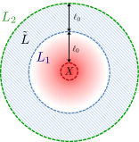
Figure 2: Schematic picture of the region where the boson number is truncated. In the region $L_{1}$ ($=X[\ell_{0}]$), we cannot restrict the boson number distribution. On the other hand, as long as $\ell_{0}$ is sufficiently large, the boson number outside $L_{1}$ can be truncated up to a finite value $q$. We perform the boson number truncation in the shaded region $\tilde{L}=L_{2}\setminus L_{1}$ with $L_{2}=X[2\ell_{0}]$. By using an effective Hamiltonian $\tilde{H}[\tilde{L},q]$ as in Eq. (18), we can approximate the exact dynamics by choosing the appropriate $q$ [i.e., $\eta\ell_{0}$; see the inequality (Lieb-Robinson bound and almost-linear light-cone in interacting boson systems)].

In the second technique, we construct an effective Hamiltonian that has bounded local energy in a specific region and approximates the exact dynamics (see Sec. S.VII. in Supplementary materials [94]). The inequality (16) implies that the boson number $\hat{n}_{i}$ is strongly suppressed when the site $i$ is sufficiently separated from the region $X$. Hence, we expect that, in the original Hamiltonian $H$, the maximum boson number at one site can be truncated during short-time evolution. We first define two regions $L_{1}:=X[\ell_{0}]$ and $L_{2}:=X[2\ell_{0}]$, where the length $\ell_{0}$ is appropriately chosen. We then consider the boson truncation in the region $\tilde{L}$ which is defined as (see Fig. 2)

$$\tilde{L}:=L_{2}\setminus L_{1}.$$ (17)

We now define $\bar{\Pi}_{\tilde{L},q}$ as the projection onto the eigenspace such that the boson number $\hat{n}_{i}$ ($\forall i\in\tilde{L}$) is truncated up to $q$, i.e., $\|\hat{n}_{i}\bar{\Pi}_{\tilde{L},q}\|\leq q$. We then approximate the time-evolution operator $e^{-iHt}$ by using an effective Hamiltonian $\tilde{H}[\tilde{L},q]$, defined by

$$\tilde{H}[\tilde{L},q]:=\bar{\Pi}_{\tilde{L},q}H\bar{\Pi}_{\tilde{L},q},$$ (18)

with a bounded local energy in the region $\tilde{L}$. In general, the time evolution $O_{X}(t)$ cannot be approximated by $O_{X}(\tilde{H}[\tilde{L},q],t)$ at all, where we have used the notation (3). However, we are only interested in the norm difference between $O_{X}(t)\rho_{0}$ and $O_{X}(\tilde{H}[\tilde{L},q],t)\rho_{0}$. We can prove

$$\left\|\left[O_{X}(t)-O_{X}(\tilde{H}[\tilde{L},\eta\ell_{0}],t)\right]\rho_{0}\right\|_{1}$$

$$\leq\frac{\|O_{X}\|}{2}e^{c_{0}\bar{q}}e^{-2\ell_{0}/\log(r)}$$ (19)

for $q=\eta\ell_{0}$ and $\ell_{0}\geq C_{0}\log^{2}(r)$, where $\eta$ and $C_{0}$ are $\mathcal{O}(1)$ constants which are independent of $\bar{q}$, and $r$ has been defined by $X\subseteq i[r]$. From this upper bound, we can see that the error exponentially decreases with the number of the boson truncation. Thus, by using the Hamiltonian $\tilde{H}[\tilde{L},\eta\ell_{0}]$, the biggest obstacle, namely the unboundedness of the interaction norms, has been removed, at least in the region $\tilde{L}$. However, outside this region, the norm is still unbounded. We thus need to consider how to derive the Lieb–Robinson bound for $e^{-i\tilde{H}[\tilde{L},\eta\ell_{0}]t}$ only from the finiteness of the Hamiltonian norm in the region $\tilde{L}$.

Our final task is to approximate the time evolution $O_{X}(\tilde{H}[\tilde{L},\eta\ell_{0}],t)$ by $U_{L_{2}}^{\dagger}O_{X}U_{L_{2}}$, where $U_{L_{2}}$ is an appropriate unitary operator supported on the subset $L_{2}$ (see Sec. S.VIII. in Supplementary materials [94]). By a careful calculation based on the standard approach to deriving the Lieb–Robinson bound, we can show that the approximation error obeys

$$\left\|O_{X}(\tilde{H}[\tilde{L},\eta\ell_{0}],t)-U_{L_{2}}^{\dagger}O_{X}U_{L_{2}}\right\|\leq\frac{\|O_{X}\|}{2}e^{-2\ell_{0}/\log(r)},$$ (20)

assuming $t\leq\Delta t_{0}$ with $\Delta t_{0}$ an $\mathcal{O}(1)$ constant. Therefore, under the conditions $\ell_{0}\geq C_{0}\log^{2}(r)$ and $t\leq\Delta t_{0}$, we have the inequalities (Lieb-Robinson bound and almost-linear light-cone in interacting boson systems) and (20), which together yield the desired inequality (Lieb-Robinson bound and almost-linear light-cone in interacting boson systems) since $e^{c_{0}\bar{q}}\geq 1$.

Conclusion.— In this work, we have established the Lieb–Robinson bound (Lieb-Robinson bound and almost-linear light-cone in interacting boson systems) with an almost-linear light cone $R\propto t\log^{2}(t)$ for arbitrary initial steady states under the condition (6). Our bound leads to the clustering theorem (8) for gapped ground states and the efficient simulation of the quench dynamics as in (10). Our result gives the first rigorous characterization of the light cone of interacting boson systems under experimentally realistic conditions.

Nevertheless, this Lieb–Robinson bound might be further improved. First, the asymptotic form $e^{-R/(t\log R)}$ in (Lieb-Robinson bound and almost-linear light-cone in interacting boson systems) could be changed to $e^{-R+vt}$, which would induce a strictly linear light cone for information propagation. Second, there remains the challenge to clarify the class of quantum states that rigorously satisfy the assumption (6). Third, regarding the time independence of $\rho_{0}$, we conjecture that an information wave-front of at least polynomial form (i.e., $R\propto t^{\zeta}$, $\zeta\geq 1$) can be derived when $\rho_{0}$ is time-dependent. Although our current techniques cannot immediately accommodate these improvements, we hope to develop a better Lieb–Robinson bound for interacting bosons in the future.

Note added. For the readers information, we would like to refer to a subsequent study by Yin and Lucas [96], which proves the linear light cone for interacting boson systems in another specific setup.

S.I Set up

We first describe the setup, which is described in less detail in the main text.

We consider a quantum system on a $D$-dimensional lattice (graph), where bosons interact with each other. An unbounded number of bosons occupy each site, and hence the local Hilbert dimension is infinitely large. We define $d_{G}$ as the maximum degree of the lattice (graph). We denote the set of total sites by $\Lambda$. For an arbitrary partial set $X\subseteq\Lambda$, we denote the cardinality (i.e., the number of sites contained in $X$) by $|X|$.

For arbitrary subsets $X,Y\subseteq\Lambda$, we define $d_{X,Y}$ as the shortest path length on the graph that connects $X$ and $Y$; that is, if $X\cap Y\neq\emptyset$, $d_{X,Y}=0$. When $X$ contains only one element (i.e., $X=\{i\}$), we abbreviate $d_{\{i\},Y}$ as $d_{i,Y}$ for simplicity. We also denote the complementary subset and surface subset of $X$ by $X^{\rm c}:=\Lambda\setminus X$ and $\partial X:=\{i\in X|d_{i,X^{\rm c}}=1\}$, respectively. We also define ${\rm diam}(X)$ as follows:

$${\rm diam}(X):=1+\max_{i,j\in X}(d_{i,j}).$$ (S.2)

For a subset $X\subseteq\Lambda$, we define the extended subset $X[r]$ as

$$X[r]:=\{i\in\Lambda|d_{X,i}\leq r\},$$ (S.3)

where $X[0]=X$, and $r$ is an arbitrary positive number (i.e., $r\in\mathbb{R}^{+}$). From the definition, $i[r]$ is given by a ball region with radius $r$ centered at the site $i$. We introduce a geometric parameter $\gamma$, which is determined only by the lattice structure. We define $\gamma\geq 1$ as a constant of $\mathcal{O}(1)$ that satisfies the following inequalities:

$$|i[r]|\leq\gamma r^{D}\quad(r\geq 1).$$ (S.4)

We define the constant $\lambda_{0}$ as follows:

$$\lambda_{0}:=\max_{i\in\Lambda}\sum_{j\in\Lambda}e^{-d_{i,j}}.$$ (S.5)

The parameter $\lambda_{0}$ depends on $\gamma$ and $D$ because, when the parameter $\gamma$ is used, it is upper-bounded as

$$\sum_{j\in\Lambda}e^{-d_{i,j}} =1+\sum_{x=1}^{\infty}\sum_{j:d_{i,j}=x}e^{-x}$$

$$\leq 1+\gamma\sum_{x=1}^{\infty}x^{D}e^{-x}\leq 1+\gamma\int_{0}^{\infty}x^{D}e^{-x+1}dx=1+e\gamma D!,$$ (S.6)

where we use the inequality $\#\{j:d_{i,j}=x\}\leq\#\{j:d_{i,j}\leq x\}=|i[x]|\leq\gamma x^{D}$.

S.I.1 Boson operators

We define $b_{i}$ and $b_{i}^{\dagger}$ as the boson annihilation and creation operators, respectively. We also define $\hat{n}_{i}$ as the boson number operator on site $i$, $\hat{n}_{i}:=b_{i}^{\dagger}b_{i}$. We denote the boson number on a subset $X$ by $\hat{n}_{X}$ as follows:

$$\hat{n}_{X}=\sum_{i\in X}\hat{n}_{i}.$$ (S.7)

For an arbitrary subset $X\subseteq\Lambda$, we define $\Pi_{X,q}$ as the projection onto the eigenspace of $\hat{n}_{X}$ with eigenvalue $q$:

$$\hat{n}_{X}\Pi_{X,q}=q\Pi_{X,q}.$$ (S.8)

When $X$ includes only one site (i.e., $X=\{i\}$), we denote $\Pi_{\{i\},q}$ by $\Pi_{i,q}$ for simplicity. We also define $\Pi_{X,\geq q}$ as $\sum_{q^{\prime}=q}^{\infty}\Pi_{X,q^{\prime}}$.

S.I.2 Bose-Hubbard type Hamiltonian

We consider a Hamiltonian of the form

$$H=H_{0}+V,$$

$$H_{0}:=\sum_{\langle i,j\rangle}J_{i,j}(b_{i}b_{j}^{\dagger}+{\rm h.c.}),\quad V:=\sum_{Z\subset\Lambda:|Z|\leq k}v_{Z},$$

$$|J_{i,j}|\leq\bar{J},$$ (S.9)

where $\sum_{\langle i,j\rangle}$ represents the summation of all the pairs of adjacent sites $\{i,j\}$ on the lattice, and $v_{Z}$ represents boson–boson interactions in subset $Z$. We assume that $v_{Z}$ is now given by a function of the number operators $\{\hat{n}_{i}\}_{i\in Z}$. For example, for $Z=\{i,j\}$, $v_{Z}$ includes interactions such as $\hat{n}_{i}^{4}$, $\hat{n}_{i}^{2}e^{\hat{n}_{j}}$, $e^{\hat{n}_{i}^{2}\hat{n}_{j}^{3}}$, and so on. The simplest example is the Bose–Hubbard model:

$$H=\sum_{\langle i,j\rangle}J(b_{i}b_{j}^{\dagger}+{\rm h.c.})+\frac{U}{2}\sum_{i\in\Lambda}\hat{n}_{i}(\hat{n}_{i}-1)-\mu\sum_{i\in\Lambda}\hat{n}_{i},$$ (S.10)

where $U$ and $\mu$ are $\mathcal{O}(1)$ constants.

For an arbitrary subset $X\subseteq\Lambda$, we define the subset Hamiltonians $H_{0,X}$, $V_{X}$, and $H_{X}$ as follows:

$$H_{X}=H_{0,X}+V_{X},$$

$$H_{0,X}:=\sum_{i,j\in X}[J_{i,j}(b_{i}b_{j}^{\dagger}+{\rm h.c.})],\quad V_{X}:=\sum_{Z\subseteq X:|Z|\leq k}v_{Z}.$$ (S.11)

Note that they are supported on the subset $X$.

For an arbitrary operator $O$, we denote the time evolution by an operator $A$ as $O(A,t)$ as follows:

$$O(A,t):=e^{iAt}Oe^{-iAt}.$$ (S.12)

In particular, when $A=H$, we often abbreviate $O(H,t)$ as $O(t)$ for simplicity.

We define $t_{0}$ as the unit of time, which is an $\mathcal{O}(1)$ constant; for example, we can choose $t_{0}=1$.

S.I.3 Initial condition for the boson density

We here define the condition of low boson density as follows.

Assumption 1 (Low boson density).

For a quantum state $\sigma$, we say that the state $\sigma$ satisfies the low-boson-density condition if there exist $\mathcal{O}(1)$ constants $c_{0}$ and $\bar{q}$ such that

$$\max_{i\in\Lambda}{\rm tr}(e^{c_{0}(\hat{n}_{i}-\bar{q})}\sigma)\leq 1\quad(c_{0}\leq 1).$$ (S.13)

This condition ensures that the probability that many bosons are concentrated on one site is exponentially small. Indeed, the probability that $\sigma$ has more than $q$ ($q\in\mathbb{N}$) bosons on a site $i$ is upper-bounded by

$${\rm tr}(\Pi_{i,\geq q}\rho_{0}) ={\rm tr}\left(\Pi_{i,\geq q}e^{-c_{0}(\hat{n}_{i}-\bar{q})/2}e^{c_{0}(\hat{n}_{i}-\bar{q})/2}\rho_{0}e^{c_{0}(\hat{n}_{i}-\bar{q})/2}e^{-c_{0}(\hat{n}_{i}-\bar{q})/2}\Pi_{i,\geq q}\right)$$

$$\leq\|\Pi_{i,\geq q}e^{-c_{0}(\hat{n}_{i}-\bar{q})/2}\|^{2}\cdot{\rm tr}(e^{c_{0}(\hat{n}_{i}-\bar{q})}\rho_{0})\leq e^{-c_{0}(q-\bar{q})}.$$ (S.14)

In the first inequality, we use the inequality ${\rm tr}(O^{\dagger}AO)\leq\|O\|^{2}{\rm tr}(A)$ for an arbitrary positive operator $A$. Therefore, the probability decays exponentially beyond $q\approx\bar{q}$.

Remark. This condition is expected to hold in real experimental setups, although it would be difficult to prove rigorously in general. Quantum Gibbs states are among the candidates that satisfy the condition; as a trivial example, our theory can be applied to the infinite-temperature state. If we specify a setup (e.g., that there exists a repulsive force between bosons), we could prove the condition (S.13) for low-energy states by employing the techniques in [97].

S.II Main result: Lieb–Robinson bound for interacting bosons

Let $\rho_{0}$ be a time-independent quantum state, $[\rho_{0},H]=0$. We then consider the propagation of a perturbation to $\rho_{0}$ as

$$\rho=O_{X_{0}}\rho_{0}O_{X_{0}}^{\dagger},\quad X\subseteq i_{0}[r_{0}].$$ (S.15)

We are now interested in how fast this perturbation propagates. After time evolution, $\rho(t)$ is given mathematically by $O_{X_{0}}(t)\rho_{0}O_{X_{0}}(t)^{\dagger}$, and hence we need to estimate the approximation error of

$$O_{X_{0}}(t)\rho_{0}\approx O^{(t)}_{i_{0}[R]}\rho_{0},$$ (S.16)

where $O^{(t)}_{i_{0}[R]}$ is an appropriate operator supported on the subset $i_{0}[R]$. We aim to upper-bound the error as a function of $R$ (Fig. 3).

In deriving the Lieb–Robinson bound, we need to assume that boson creation by $O_{X_{0}}$ is not infinitely large; thus, we adopt the following condition:

$$\|\Pi_{X_{0},q}O_{X_{0}}\Pi_{X_{0},q^{\prime}}\|=0\quad\textrm{for}\quad q^{\prime}>q+q_{0}$$ (S.17)

with $q_{0}=\mathcal{O}(1)$, where the projection $\Pi_{X_{0},q}$ has been defined by Eq. (S.8). The above condition implies that the number of bosons created by $O_{X_{0}}$ is less than or equal to $q_{0}$. We notice that the above condition also implies

$$\|\Pi_{X,q}O_{X_{0}}\Pi_{X,q^{\prime}}\|=0\quad\textrm{for}\quad q^{\prime}>q+q_{0}$$ (S.18)

for an arbitrary subset $X\supseteq X_{0}$.

Our main result gives the Lieb–Robinson bound for an arbitrary quantum state $\rho_{0}$ satisfying the low-boson-density condition (1).

Theorem 1.

Let $O_{X_{0}}$ be an arbitrary operator supported on a subset $X_{0}\subseteq i_{0}[r_{0}]$ ($i_{0}\in\Lambda$). We assume that the number of bosons created by $O_{X_{0}}$ is finite, as in Eq. (S.17). Then, for an arbitrary steady quantum state $\rho_{0}$ satisfying the assumption (1), the operator $O_{X_{0}}(t)\rho_{0}$ is approximated by using another operator $O^{(t)}_{i_{0}[R]}$ supported on $i_{0}[R]$ with the following approximation error:

$$\left\|\left(O_{X_{0}}(t)-O^{(t)}_{i_{0}[R]}\right)\rho_{0}\right\|_{1}\leq\|O_{X_{0}}\|\exp\left(c_{0}\bar{q}-C_{1}\frac{(R-r_{0})}{t\log(R)}+C_{2}\log(R)\right)\quad(t\geq 1),$$ (S.20)

where $C_{1}$ and $C_{2}$ are constants of $\mathcal{O}(1)$ which are independent of $\bar{q}$ and depend only on the details of the system.

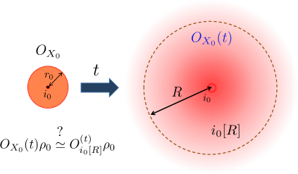
Figure 3: Schematic illustration of Theorem 1.

Remark. From the above result, we can identify the shape of the effective light cone. We here assume $t\geq e$ and $X_{0}=i_{0}$ ($r_{0}=0$) for simplicity. As shown in the main text, the velocity $v_{t,\delta}$ to characterize the effective light cone has been defined by the following inequality:

$$\|[O_{i_{0}}(t)-O^{(t)}_{i_{0}[R]}]\|\leq\delta\left\|O_{i_{0}}\right\|\quad\textrm{for}\quad R\geq v_{t,\delta}|t|.$$ (S.21)

In order to achieve the above inequality for a particular choices of $t$ and $\delta$, we need to choose $R$ such that

$$\exp\left(c_{0}\bar{q}-C_{1}\frac{R}{t\log(R)}+C_{2}\log(R)\right)\leq\delta$$

$$\longrightarrow C_{1}\frac{R}{t\log(R)}-C_{2}\log(R)\geq c_{0}\bar{q}+\log(1/\delta)\longrightarrow\frac{R}{t\log(R)}-\tilde{C}_{2}\log(R)\geq Q,$$ (S.22)

where we define $\tilde{C}_{2}:=C_{2}/C_{1}$ and $Q=[c_{0}\bar{q}+\log(1/\delta)]/C_{1}$. We now choose $R=\Gamma t\log^{2}(t)$ by using a parameter $\Gamma$ ($\geq 1$). Then, from $\Gamma t\leq R\leq\Gamma t^{2}$ for $t\geq e$, we obtain the condition of

$$\Gamma\log(t)-2\tilde{C}_{2}\log(t)-\tilde{C}_{2}\log(\Gamma)\geq Q.$$ (S.23)

Let $\Gamma_{c}$ be a constant depending on $\tilde{C}_{2}$ such that $(1/2)\Gamma\geq\tilde{C}_{2}\log(\Gamma)$ for $\Gamma\geq\Gamma_{c}$. Then, for $\Gamma\geq\Gamma_{c}$, the condition (S.25) reduces to

$$\Gamma(\log(t)-1/2)\geq 2\tilde{C}_{2}\log(t)+Q\longrightarrow\Gamma\geq\frac{2\tilde{C}_{2}\log(t)+Q}{\log(t)-1/2}\longrightarrow\Gamma\geq 4\tilde{C}_{2}+2Q,$$ (S.24)

where the last inequality results from $t\geq e$. Therefore, by choosing

$$R=t\log^{2}(t)\max(\Gamma_{c},4\tilde{C}_{2}+2Q)=t\log^{2}(t)\max\left(\Gamma_{c},4C_{2}/C_{1}+2[c_{0}\bar{q}+\log(1/\delta)]/C_{1}\right),$$ (S.25)

the inequality (S.21) is satisfied. We thus conclude that $v_{t,\delta}\propto\log^{2}(t)[c_{0}\bar{q}+\log(1/\delta)]$.

S.III Clustering theorem for gapped ground states

As a direct application of Theorem 1, we can discuss the clustering property of the bipartite correlations in gapped ground states. Let $\{|E_{j}\rangle\}_{j\geq 0}$ be eigenstates of the Hamiltonian $H$. We set $E_{0}=0$ and define $\Delta E:=E_{1}$ as the spectral gap between the ground and first excited energies. We can prove the following corollary.

Corollary 2.

Let $O_{X}$ and $O_{Y}$ be arbitrary operators satisfying the condition (S.17) for a fixed $q_{0}$. Also, we here assume that $\bar{q}=\mathcal{O}(1)$. Then, for the ground states $|E_{0}\rangle$ with low boson density according to Eq. (1), the bipartite correlation between $O_{X}$ and $O_{Y}$ satisfies the inequality

$${\rm Cor}(O_{X},O_{Y}):=\langle E_{0}|O_{X}O_{Y}|E_{0}\rangle-\langle E_{0}|O_{X}|E_{0}\rangle\langle E_{0}|O_{Y}|E_{0}\rangle\leq C_{3}\cdot\|O_{X}\|\cdot\|O_{Y}\|\cdot\exp\left(-\sqrt{\frac{C_{3}^{\prime}\Delta E}{\log(R)}R}\right)$$ (S.26)

for $R\geq{\rm const.}\times(1/\Delta E)\log^{3}(1/\Delta E)$. Here, $C_{3}$ and $C_{3}^{\prime}$ are $\mathcal{O}(1)$ constants.

Remark. According to this corollary, the correlation decays sub-exponentially with $R$ that is larger than $\tilde{\mathcal{O}}(1/\Delta E)$. This corollary is weaker than the standard clustering theorem [4, 5, 6], which yields exponential decay of the bipartite correlations as $e^{-\mathcal{O}(\Delta ER)}$. The primary reason is that the asymptotic form of the Lieb–Robinson bound in Theorem 1 is given by $e^{-\mathcal{O}(R/(t\log R))}$ instead of $e^{-\mathcal{O}(R-vt)}$. This point is reflected in the choice of $T$ in Eqs. (S.32), (S.34), and (S.35) below. For example, if we could improve the present upper bound to $e^{-\mathcal{O}(R/(\log R)-vt)}$, we would be able to obtain nearly exponential decay of the bipartite correlations as $e^{-\mathcal{O}(\Delta ER/(\log R))}$.

S.III.1 Proof of Corollary 2

The proof relies on the method in Refs. [4, 5, 6]. We start with the equation

$$\langle E_{0}|[O_{X}(t),O_{Y}]|E_{0}\rangle =\sum_{s\geq 0}\left(e^{-iE_{s}t}\langle E_{0}|O_{X}|E_{s}\rangle\langle E_{s}|O_{Y}|E_{0}\rangle-e^{iE_{s}t}\langle E_{0}|O_{Y}|E_{s}\rangle\langle E_{s}|O_{X}|E_{0}\rangle\right)$$

$$=\sum_{s\geq 1}\left(e^{-iE_{s}t}\langle E_{0}|O_{X}|E_{s}\rangle\langle E_{s}|O_{Y}|E_{0}\rangle-e^{iE_{s}t}\langle E_{0}|O_{Y}|E_{s}\rangle\langle E_{s}|O_{X}|E_{0}\rangle\right).$$ (S.27)

Using the function $K(t)$, where

$$K(t)=\frac{i}{2\pi}\lim_{\epsilon\to+0}\frac{e^{-\alpha t^{2}}}{t+i\epsilon},$$ (S.28)

we have, from Ref. [5],

$$\int_{-\infty}^{\infty}e^{-i\omega t}K(t)dt=\begin{cases}{\rm const}\cdot e^{-\omega^{2}/(4\alpha)}&\quad\textrm{for}\quad\omega>0,\\ 1+{\rm const}\cdot e^{-\omega^{2}/(4\alpha)}&\quad\textrm{for}\quad\omega<0.\end{cases}$$

Here, $\alpha$ is a free parameter. Because $K(t)$ decays as $e^{-\alpha t^{2}}$, we can obtain

$$\int_{-T}^{T}e^{-i\omega t}K(t)dt =\begin{cases}{\rm const}\cdot\left(e^{-\omega^{2}/(4\alpha)}+c_{\alpha,T}e^{-\alpha T^{2}}\right)&\quad\textrm{for}\quad\omega>0,\\ 1+{\rm const}\cdot\left(e^{-\omega^{2}/(4\alpha)}+c_{\alpha,T}e^{-\alpha T^{2}}\right)&\quad\textrm{for}\quad\omega<0,\end{cases}$$

$$=\begin{cases}{\rm const}\cdot(e^{-T\omega^{2}/(2\Delta E)}+c_{\Delta E,T}e^{-T\Delta E/2})&\quad\textrm{for}\quad\omega>0,\\ 1+{\rm const}\cdot(e^{-T\omega^{2}/(2\Delta E)}+c_{\Delta E,T}e^{-T\Delta E/2})&\quad\textrm{for}\quad\omega<0,\end{cases}$$ (S.29)

where $c_{\alpha,T}$ and $c_{\Delta E,T}$ are appropriate constants, and we choose $\alpha=\Delta E/(2T)$. We note that $|c_{\Delta E,T}|\leq{\rm const.}/\sqrt{\alpha}={\rm const.}\sqrt{2T/\Delta E}$.

By applying Eq. (S.29) to Eq. (S.27), we obtain

$$\int_{-T}^{T}K(t)\langle E_{0}|[O_{X}(t),O_{Y}]|E_{0}\rangle dt$$

$$=\int_{-T}^{T}K(t)\sum_{s\geq 1}\left(e^{-iE_{s}t}\langle E_{0}|O_{X}|E_{s}\rangle\langle E_{s}|O_{Y}|E_{0}\rangle-e^{iE_{s}t}\langle E_{0}|O_{Y}|E_{s}\rangle\langle E_{s}|O_{X}|E_{0}\rangle\right)dt$$

$$=\sum_{s\geq 1}\left[K_{E_{s},\Delta E}\langle E_{0}|O_{X}|E_{s}\rangle\langle E_{s}|O_{Y}|E_{0}\rangle+(1+K_{E_{s},\Delta E})\langle E_{0}|O_{Y}|E_{s}\rangle\langle E_{s}|O_{X}|E_{0}\rangle\right]$$

$$=(\langle E_{0}|O_{X}Q_{T}O_{Y}|E_{0}\rangle+{\rm c.c.})+\sum_{s\geq 1}\langle E_{0}|O_{Y}|E_{s}\rangle\langle E_{s}|O_{X}|E_{0}\rangle,$$ (S.30)

where we set $K_{\omega,\Delta E}:={\rm const}\cdot(e^{-T\omega^{2}/(2\Delta E)}+c_{\Delta E,T}e^{-T\Delta E/2})$ and define $Q_{T}$ as

$$Q_{T}:=\sum_{s\geq 1}K_{E_{s},\Delta E}|E_{s}\rangle\langle E_{s}|.$$ (S.31)

By combining Eqs. (S.29) and (S.30), we obtain

$$\left|{\rm Cor}(O_{X},O_{Y})\right| \leq\int_{-T}^{T}K(t)|\langle E_{0}|[O_{X}(t),O_{Y}]|E_{0}\rangle|dt+{\rm const}\cdot c_{\Delta E,T}\|O_{X}\|\cdot\|O_{Y}\|\cdot e^{-T\Delta E/2},$$ (S.32)

where we use $\sum_{s\geq 1}\langle E_{0}|O_{Y}|E_{s}\rangle\langle E_{s}|O_{X}|E_{0}\rangle={\rm Cor}(O_{X},O_{Y})$ and $\|Q_{T}\|\leq K_{E_{1},\Delta E}={\rm const}\cdot c_{\Delta E,T}e^{-T\Delta E/2}$ from $\Delta E=E_{1}$. From Theorem 1, we have

$$|\langle E_{0}|[O_{X}(t),O_{Y}]|E_{0}\rangle|\leq\|[O_{X}(t),O_{Y}]\|\leq\|O_{X}\|\cdot\|O_{Y}\|\cdot\exp\left(-{\rm const}\cdot\frac{R}{t\log(R)}\right)$$ (S.33)

for $R\geq{\rm const}\cdot t\log^{2}(t)$. Hence, for $R\geq{\rm const}\cdot T\log^{2}(T)$, we obtain

$$\int_{-T}^{T}K(t)|\langle E_{0}|[O_{X}(t),O_{Y}]|E_{0}\rangle|dt\leq{\rm const}\cdot\|O_{X}\|\cdot\|O_{Y}\|\cdot T\exp\left(-{\rm const}\cdot\frac{R}{T\log(R)}\right).$$ (S.34)

We thus choose $T$ as

$$T=\sqrt{\frac{{\rm const}\cdot R}{\Delta E\log(R)}},$$ (S.35)

and we obtain the main inequality (S.26). Finally, the condition $R\geq{\rm const}\cdot T\log^{2}(T)$ reduces to

$$R\log R\geq{\rm const}\cdot\frac{1}{\Delta E}[\log^{4}(R)+\log^{4}(1/\Delta E)],$$ (S.36)

which is satisfied if $R\geq{\rm const}\cdot(1/\Delta E)\log^{3}(1/\Delta E)$. This completes the proof. $\square$

S.IV Proof outline of the main theorem (Fig. 4)

S.IV.1 Lieb–Robinson bound for short-time evolution

The key ingredient in our proof is the Lieb–Robinson bound for short-time evolution. We consider a quantum state $\tilde{\rho}$, which is defined using an operator $O_{X}$ supported on a subset $X\subset\Lambda$:

$$\tilde{\rho}:=O_{X}\rho_{0}O_{X}^{\dagger},\quad X\in i_{0}[r]\quad(i_{0}\in\Lambda,\ r\geq 3),$$ (S.37)

where $O_{X}$ is given in the form

$$O_{X}=U_{X}^{\dagger}O_{X_{0}}U_{X},\quad[U_{X},\hat{n}_{X}]=0,$$ (S.38)

where $U_{X}$ is a unitary operator that commutes with $\hat{n}_{X}$. Because $O_{X_{0}}$ satisfies the condition (S.17), and $U_{X}$ does not change the total number of bosons on $X$, we obtain

$$\|\Pi_{X,q}O_{X}\Pi_{X,q^{\prime}}\|=0\quad\textrm{for}\quad q^{\prime}>q+q_{0}.$$ (S.39)

We are now interested in the approximation

$$O_{X}(t)\rho_{0}\approx(U_{X[\ell]}^{\dagger}O_{X}U_{X[\ell]})\rho_{0}$$ (S.40)

for a sufficiently small $t=\mathcal{O}(1)$, where $U_{X[\ell]}$ is an appropriate unitary operator defined on the subset $X[\ell]$. We can prove the following statement about the approximation.

Subtheorem 1.

Let $O_{X}$ be an arbitrary operator as defined in Eq. (S.38), which is supported on the subset $X\subseteq i_{0}[r]$ ($i_{0}\in\Lambda$). Then, for a length $\ell$ that satisfies

$$\ell\geq C_{0}\log^{2}(r),$$ (S.41)

with $C_{0}=\mathcal{O}(1)$ which does not depend on $\bar{q}$, we can find a unitary operator $U_{X[\ell]}$ that does not depend on the form of $O_{X}$ such that

$$[U_{X[\ell]},\hat{n}_{X[\ell]}]=0$$ (S.42)

and

$$\left\|\left(O_{X}(t)-U_{X[\ell]}^{\dagger}O_{X}U_{X[\ell]}\right)\rho_{0}\right\|_{1}\leq\|O_{X}\|e^{c_{0}\bar{q}-\ell/\log(r)}$$ (S.43)

for $t\leq\Delta t_{0}$, where $\Delta t_{0}=\mathcal{O}(1)$ and $C_{0}$ are appropriately chosen. We can combine condition (S.41) with Ineq. (S.43) as follows:

$$\left\|\left(O_{X}(t)-U_{X[\ell]}^{\dagger}O_{X}U_{X[\ell]}\right)\rho_{0}\right\|_{1}\leq\|O_{X}\|e^{c_{0}\bar{q}-\ell/\log(r)+C_{0}\log(r)},$$ (S.44)

where the inequality holds trivially for $\ell\leq C_{0}\log^{2}(r)$.

Remark. In this subtheorem, we do not need to assume the time-independence of the state $\rho_{0}$. Hence, only the assumption 1 is used. When $\rho_{0}$ does not satisfy $[\rho_{0},H]=0$, Ineq. (S.43) is replaced by

$$\left\|\left(O_{X}(t)-U_{X[\ell]}^{\dagger}O_{X}U_{X[\ell]}\right)\rho_{0}(-t)\right\|_{1}\leq\|O_{X}\|e^{c_{0}\bar{q}-\ell/\log(r)}.$$ (S.45)

By contrast, when we prove the main theorem, we need to connect the short-time evolutions, and to perform this procedure, the time-independence of $\rho_{0}$ is required [see Eqs. (S.IV.2) and (S.53)].

It is necessary to generalize Eq. (S.45) when applying the subtheorem to analyze the quench dynamics (see Sec. S.IX).

S.IV.2 Proof of Theorem 1 based on Subtheorem 1

For the convenience of readers, we present the approach to the proof in the main text again with additional explanations. We use the connection of unitary time evolutions addressed in Refs. [95, 29], which assumes the time-independence of the initial state (i.e., $\rho_{0}(t)=\rho_{0}$).

We introduce $\Delta t\leq\Delta t_{0}$ and the following decompositions of the time $t$ to $t/\Delta t$ pieces:

$$t:=m_{t}\Delta t\quad{\rm with}\quad\Delta t\geq\min(t,\Delta t_{0}/2).$$ (S.46)

For fixed $R$, we define the subset $X_{m}$ as follows:

$$X_{m}:=i_{0}[r_{0}+m\Delta r]=X_{0}[m\Delta r],\quad\Delta r=\left\lfloor\frac{R-r_{0}}{m_{t}}\right\rfloor.$$ (S.47)

Note that $X_{m_{t}}\subseteq i_{0}[R]$.

Then, assuming that $\rho_{0}$ is time-invariant, we can derive the following inequality [29]:

$$\left\|\left[O_{X_{0}}(m_{t}\Delta t)-O_{X_{m_{t}}}^{(m_{t})}\right]\rho_{0}\right\|_{1} \leq\sum_{m=1}^{m_{t}}\left\|\left[O_{X_{m-1}}^{(m-1)}(\Delta t)-O_{X_{m}}^{(m)}\right]\rho_{0}\right\|_{1},$$ (S.48)

where $O_{X_{0}}^{(0)}=O_{X_{0}}$, and $O_{X_{m}}^{(m)}$ is recursively defined by approximating $O_{X_{m-1}}^{(m-1)}(\Delta t)$. To see why the time-invariance of $\rho_{0}$ is essential, let us look at the derivation of Ineq. (S.48) for $m_{t}=2$. For $m=1$, we define

$$O_{X_{1}}^{(1)}:=U_{X_{1}}^{(1)\dagger}O_{X_{0}}U_{X_{1}}^{(1)},$$ (S.49)

where we choose the unitary operator $U_{X_{1}}$ by following Subtheorem 1. Note that $O_{X_{1}}^{(1)}$ is now supported on the subset $X_{1}$. For $m=2$, we consider the approximation $O_{X_{1}}^{(1)}(\Delta t)$ by

$$O_{X_{2}}^{(2)}:=U_{X_{2}}^{(2)\dagger}O_{X_{1}}^{(1)}U_{X_{2}}^{(2)},$$ (S.50)

where the unitary operator $U_{X_{2}}^{(2)}$ is chosen according to Subtheorem 1. We then connect the two approximations:

$$O_{X_{0}}(\Delta t)\xrightarrow{\rm approximate}O_{X_{1}}^{(1)},\quad O_{X_{1}}^{(1)}(\Delta t)\xrightarrow{\rm approximate}O_{X_{2}}^{(2)}.$$ (S.51)

To obtain the approximation error, we need to consider

$$\left\|\left[O_{X_{0}}(2\Delta t)-O_{X_{2}}^{(2)}\right]\rho_{0}\right\|_{1} \leq\left\|\left[O_{X_{0}}(2\Delta t)-O_{X_{1}}^{(1)}(\Delta t)+O_{X_{1}}^{(1)}(\Delta t)-O_{X_{2}}^{(2)}\right]\rho_{0}\right\|_{1}$$

$$\leq\left\|\left[O_{X_{0}}(2\Delta t)-O_{X_{1}}^{(1)}(\Delta t)\right]\rho_{0}\right\|_{1}+\left\|\left[O_{X_{1}}^{(1)}(\Delta t)-O_{X_{2}}^{(2)}\right]\rho_{0}\right\|_{1}.$$ (S.52)

The second term is upper-bounded according to Subtheorem 1. The first term is given by

$$\left\|\left[O_{X_{0}}(2\Delta t)-O_{X_{1}}^{(1)}(\Delta t)\right]\rho_{0}\right\|_{1}=\left\|\left[O_{X_{0}}(\Delta t)-O_{X_{1}}^{(1)}\right]\rho_{0}(-\Delta t)\right\|_{1}.$$ (S.53)

If $\rho_{0}(-\Delta t)=\rho_{0}$, we can upper-bound the above quantity using Subtheorem 1. However, when $\rho_{0}$ is time-dependent, the condition (1) for low boson density may not be satisfied for $\rho_{0}(-\Delta t)$. Therefore, to prove the main theorem for generic $\rho_{0}$, we need to prove the low-boson-density condition for $\rho_{0}(-m\Delta t)$ ($m\leq m_{t}-1$).

We return to Ineq. (S.48). According to Subtheorem 1, we can find $O_{X_{m}}^{(m)}$ such that

$$O_{X_{m}}^{(m)}:=U_{X_{m}}^{(m)\dagger}O_{X_{m-1}}^{(m-1)}U_{X_{m}}^{(m)}$$ (S.54)

for each $m=1,2,\ldots,m_{t}$. From Ineq. (S.44), the unitary operator $U_{X_{m}}^{(m)}$ satisfies

$$\left\|\left(U_{X_{m}}^{(m)\dagger}O_{X_{m-1}}^{(m-1)}U_{X_{m}}^{(m)}-O_{X_{m-1}}^{(m-1)}(\Delta t)\right)\rho_{0}\right\|_{1}\leq\|O_{X_{0}}\|e^{c_{0}\bar{q}-\Delta r/\log(R)+C_{0}\log(R)},$$ (S.55)

where we use $X_{m}\subseteq i_{0}[R]$ for all $m$ in applying Subtheorem 1. We thus obtain

$$\left\|\left[O_{X_{0}}(m_{t}\Delta t)-O_{X_{m_{t}}}^{(m_{t})}\right]\rho_{0}\right\|_{1} \leq m_{t}\|O_{X_{0}}\|e^{c_{0}\bar{q}-\Delta r/\log(R)+C_{0}\log(R)}$$

$$\leq\|O_{X_{0}}\|\exp\left(c_{0}\bar{q}-\frac{\Delta t(R-r_{0})}{t\log(R)}+\frac{1}{\log(R)}+(C_{0}+1)\log(R)\right),$$ (S.56)

for $R\geq 2$, where in the second inequality we use $\Delta r\geq 1$ [or $m_{t}\leq(R-r_{0})$]. Thus, because of $1/\log(R)\leq 3\log(R)$ for $R\geq 2$, by choosing $C_{1}=\Delta t$ and $C_{2}=C_{0}+4$, the inequality (S.IV.2) reduces to Ineq. (S.20). This completes the proof of Theorem 1. $\square$

In the following sections, we give the full proof of Subtheorem 1. Note that the following proof repeats some of the explanations in the main text. We show the outline of the proof in Fig. 4.

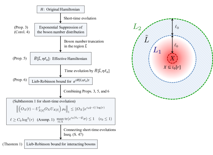
Figure 4: Schematic illustration of the proof of Theorem 1.

S.V Proof of Subtheorem 1

Here, we derive the inequality (S.45) in which the time-independence of $\rho_{0}$ is not satisfied. Throughout the proof, we denote $\|O_{X_{0}}\|$ by $\zeta_{0}$. Because of the definition (S.38) of $O_{X}$, we have

$$\|O_{X}\|=\zeta_{0}.$$ (S.57)

We first show that the following simple analysis does not work in proving the subtheorem. If short-time evolution is considered, the following simple Taylor expansion is expected to work:

$$\|[O_{X}(t),u_{i}]\rho_{0}\|_{1}=\|[O_{X},u_{i}(-t)]\rho_{0}\|_{1}=\left\|\sum_{s=0}^{\infty}\frac{(-t)^{s}}{s!}[{\rm ad}_{H}^{s}(u_{i}),O_{X}]\rho_{0}\right\|_{1}\leq\sum_{s=0}^{\bar{s}}\frac{t^{s}}{s!}\left\|[{\rm ad}_{H}^{s}(u_{i}),O_{X}]\rho_{0}\right\|_{1},$$ (S.58)

where $u_{i}$ is an arbitrary unitary operator acting on a site $i\in\Lambda$. Because the Hamiltonian is short-range, we have $[{\rm ad}_{H}^{s}(u_{i}),O_{X}]=0$ for $s\leq\bar{s}$, where $\bar{s}=\mathcal{O}(d_{i,X})$. Hence, we have

$$\|[O_{X}(t),u_{i}]\rho_{0}\|_{1}\leq\sum_{s=\bar{s}+1}^{\infty}\frac{t^{s}}{s!}\left\|[{\rm ad}_{H}^{s}(u_{i}),O_{X}]\rho_{0}\right\|_{1}.$$ (S.59)

In standard spin models with bounded local energy, we have

$$\|{\rm ad}_{H}^{s}(u_{i})\|\lesssim s!,$$ (S.60)

and hence we can ensure the exponential convergence of the expansion (S.58) for $t=\mathcal{O}(1)$. Unfortunately, this simple estimation cannot be used to obtain Subtheorem 1. When we formally describe the Hamiltonian (S.9) as

$$H=\sum_{|Z|\leq k}h_{Z},$$ (S.61)

we need to consider the norm of

$$h_{Z_{1}}h_{Z_{2}}\cdots h_{Z_{s_{1}}}u_{i}h_{Z_{s_{1}+1}}\cdots h_{Z_{s}}O_{X}\rho_{0},$$ (S.62)

where $h_{Z}$ consists of the boson hoppings $b_{i}b_{j}^{\dagger}$ and the boson–boson interactions $v_{Z}$ in Eq. (S.9). Because the boson number $\hat{n}_{i}$ on an arbitrary site is strongly suppressed in $\rho_{0}$ from Assumption 1, we have $\|h_{Z}\rho_{0}\|_{1}=\mathcal{O}(1)$. By contrast, in the state $O_{X}\rho_{0}O_{X}^{\dagger}$, all the bosons in the region $X$ can be concentrated on one site, which may give $\|\hat{n}_{i}O_{X}\rho_{0}\|_{1}\propto|X|$ for $i\in X$. We thus obtain $\|h_{Z}O_{X}\rho_{0}\|_{1}\gtrsim|X|^{\nu}$ for $Z\cap X\neq\emptyset$, where $\nu$ is a positive integer depending on the form of $v_{Z}$. Consequently, the norm $\left\|[{\rm ad}_{H}^{s}(u_{i}),O_{X}]\rho_{0}\right\|_{1}$ has a rather weaker upper bound:

$$\left\|[{\rm ad}_{H}^{s}(u_{i}),O_{X}]\rho_{0}\right\|_{1}\lesssim s!|X|^{\nu(s-\bar{s})}.$$ (S.63)

By combining the above inequality with Eq. (S.59), we can ensure the convergence of the expansion only for $t=\mathcal{O}(1/|X|^{\nu})$, which is too weak to prove Theorem 1.

In the following, we take a different route to prove Subtheorem 1 by the three steps in Secs. S.V.1, S.V.2, and S.V.3.

S.V.1 Boson density after time evolution (Proposition 3)

We first consider the boson number distribution after a short-time evolution. To this end, we need to estimate

$${\rm tr}\left[\Pi_{i,\geq z}\tilde{\rho}(t)\right],\quad\tilde{\rho}(t)=e^{-iHt}O_{X}\rho_{0}O_{X}^{\dagger}e^{iHt}=O_{X}(-t)\rho_{0}(t)O_{X}(-t)^{\dagger},$$ (S.64)

where $\Pi_{i,z}$ has been defined by Eq. (S.8). In the state $\tilde{\rho}$, the boson number $\hat{n}_{i}$ for $i\in X$ can be as large as $\mathcal{O}(|X|)$, whereas the boson number $\hat{n}_{i}$ ($i\in X^{\rm c}$) is exponentially suppressed, as shown in Eq. (S.I.3). During the time evolution, the bosons concentrated on $X$ spread outside of $X$. We expect that after a sufficiently small time, the exponential decay of the boson number still holds for sites that are sufficiently separated from $X$.

The first proposition ensures that the boson density is not seriously affected by the time evolution for $d_{i,X}\gg 1$ if the time $t$ is of $\mathcal{O}(1)$ (see Sec. S.VI for the proof).

Proposition 3.

We first define the operator $M^{(s)}_{i}(t)$ as

$$M^{(s)}_{i}(t):={\rm tr}\left[\hat{n}_{i}^{s}\tilde{\rho}(t)\right].$$ (S.65)

Then, for $t\leq t_{0}$, the following upper bound for $M^{(s)}_{i}(t)$ holds:

$$M_{i}^{(s)}(t) \leq c^{\prime}_{1}e^{c_{0}\bar{q}}\zeta_{0}^{2}|X|^{3}(c_{1}s|X|)^{s}e^{-d_{i,X}}+c^{\prime\prime}_{1}e^{c_{0}\bar{q}}\zeta_{0}^{2}(c_{1}s)^{s},$$ (S.66)

where $c_{1}$, $c^{\prime}_{1}$, and $c^{\prime\prime}_{1}$ are defined as

$$c_{1}:=e^{8\bar{J}d_{G}t_{0}}/c_{0},$$

$$c^{\prime}_{1}:=320c_{0}^{-3}e^{4\bar{J}d_{G}t_{0}+c_{0}(1+q_{0}/|X|)},$$

$$c^{\prime\prime}_{1}:=80\lambda_{0}c_{0}^{-1}e^{4\bar{J}d_{G}t_{0}+c_{0}}.$$ (S.67)

Notice that they are $\mathcal{O}(1)$ constants if $t_{0}=\mathcal{O}(1)$.

Remark. In the proof, we fully use the methods in Ref. [67], which treats the case of $s=1$. The above upper bound increases exponentially with $t$, and hence we cannot use it to upper-bound the boson density for general $t$. The key point of the proof in Sec. S.IV.2 is that we need to treat only the short-time evolution in this subtheorem. We afterward connect the short-time evolutions step by step, as in Ineq. (S.48).

In this proposition, the form of the Hamiltonian, i.e., Eq. (S.9), is essential; if the Hamiltonian includes interactions such as $\hat{n}_{i}\hat{n}_{j}b_{i}b_{j}^{\dagger}$, the above proposition breaks down even for small $t$.

By using Proposition 3, we can immediately derive the following corollary of the boson number distribution.

Corollary 4.

Let us define the boson number distribution on a site $i\in\Lambda$ as follows:

$$P_{i,\geq z_{0}}^{(t)}:=\sum_{z\geq z_{0}}{\rm tr}\left[\Pi_{i,z}\tilde{\rho}(t)\right],$$ (S.68)

where $\Pi_{i,z}$ has been defined by Eq. (S.8). Then, for arbitrary $i\in\Lambda$ such that

$$\frac{\gamma^{3}c^{\prime}_{1}}{c^{\prime\prime}_{1}}r^{3D}\leq e^{d_{i,X}/2}\to d_{i,X}\geq 2\log\left(\frac{\gamma^{3}c^{\prime}_{1}}{c^{\prime\prime}_{1}}\right)+6D\log(r)=\mathcal{O}(\log(r)),$$ (S.69)

we obtain

$$P_{i,\geq z_{0}}^{(t)}\leq 2c^{\prime\prime}_{1}e^{c_{0}\bar{q}}\zeta_{0}^{2}\left(\frac{\tilde{c}_{1}d_{i,X}}{z_{0}}\right)^{\tilde{c}^{\prime}_{1}d_{i,X}/\log(r)},$$ (S.70)

where we have defined $r$ ($\geq 3$) by $X\subseteq i_{0}[r]$ for an appropriate choice of $i_{0}\in\Lambda$ in Eq. (S.37), and $\tilde{c}_{1}$ and $\tilde{c}^{\prime}_{1}$ are constants of $\mathcal{O}(1)$.

S.V.1.1 Proof of Corollary 4

Because $X\subseteq i_{0}[r]$, we have from Ineq. (S.4)

$$|X|\leq\gamma r^{D}.$$ (S.71)

We then choose $s$ such that

$$c^{\prime}_{1}|X|^{3}(c_{1}s|X|)^{s}e^{-d_{i,X}}\leq\gamma^{3}c^{\prime}_{1}r^{3D}(\gamma c_{1}sr^{D})^{s}e^{-d_{i,X}}\leq c^{\prime\prime}_{1}(c_{1}s)^{s},$$ (S.72)

which yields

$$\frac{\gamma^{3}c^{\prime}_{1}}{c^{\prime\prime}_{1}}r^{3D}(\gamma r^{D})^{s}\leq e^{d_{i,X}/2}(\gamma r^{D})^{s}\leq e^{d_{i,X}}$$

$$\longrightarrow s\leq\frac{d_{i,X}}{2\log(\gamma r^{D})},$$ (S.73)

where we use the condition (S.69). We choose $s$ as

$$s=\left\lfloor\frac{d_{i,X}}{2\log(\gamma r^{D})}\right\rfloor\in\left[\tilde{c}^{\prime}_{1}\frac{d_{i,X}}{\log(r)},\tilde{c}_{1}^{\prime\prime}\frac{d_{i,X}}{\log(r)}\right],$$ (S.74)

where $\tilde{c}^{\prime}_{1}$ and $\tilde{c}^{\prime\prime}_{1}$ are constants which depend only on $\gamma$ and $D$. By using the inequality (S.72), we reduce the Ineq. (S.66) to

$$M_{i}^{(s)}(t) \leq 2c^{\prime\prime}_{1}e^{c_{0}\bar{q}}\zeta_{0}^{2}(c_{1}s)^{s},$$ (S.75)

and hence Markov’s inequality yields

$$P_{i,\geq z_{0}}^{(t)}\leq\frac{M_{i}^{(s)}(t)}{z_{0}^{s}}\leq 2c^{\prime\prime}_{1}e^{c_{0}\bar{q}}\zeta_{0}^{2}\left(\frac{c_{1}\tilde{c}^{\prime\prime}_{1}d_{i,X}}{z_{0}\log(r)}\right)^{\tilde{c}^{\prime}_{1}d_{i,X}/\log(r)}.$$ (S.76)

By using $\log(r)\geq 1$ from $r\geq 3$ and defining $\tilde{c}_{1}:=c_{1}\tilde{c}^{\prime\prime}_{1}$, we prove the main inequality (S.70). This completes the proof. $\square$

S.V.2 Effective Hamiltonian (Proposition 5)

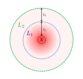
(a) Subsets $L_{1}$ and $L_{2}$

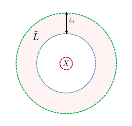
(b) Subset $\tilde{L}$

Figure 5: Schematic illustrations of sets $L_{1}$, $L_{2}$, and $\tilde{L}$. In the region $L_{1}$, we cannot ensure that the boson number distribution is exponentially localized. By contrast, if $\ell_{0}$ is sufficiently large [see the condition (S.83)], it is ensured that in the region $\tilde{L}=L_{2}\setminus L_{1}$, the boson number can be truncated up to a finite value. We define the effective Hamiltonian $\tilde{H}[\tilde{L},\eta\ell_{0}]$ using Eqs. (S.79) and (S.V.2), which well approximates the exact dynamics, as described by Ineq. (S.84).

Proposition 3 and Corollary 4 imply that during the time evolution, the boson number $\hat{n}_{i}$ is strongly suppressed as long as site $i$ is separated from the region $X$ by a sufficient distance. Hence, we expect that in the Hamiltonian $H$, the maximum boson number on one site can be truncated. In this subsection, we rigorously justify this procedure.

As shown in Fig. 5, we first define $L_{1}$ and $L_{2}$ as

$$L_{1}=X[\ell_{0}],\quad L_{2}=X[2\ell_{0}].$$ (S.77)

We also define $\tilde{L}$ as

$$\tilde{L}:=L_{2}\setminus L_{1}.$$ (S.78)

We now define $\bar{\Pi}_{L,q}$ ($L\subseteq\Lambda$) as the projection onto the eigenspace such that for an arbitrary $i\in L$, the boson number $\hat{n}_{i}$ is truncated up to $q$:

$$\bar{\Pi}_{L,q}:=\prod_{i\in L}\Pi_{i,\leq q}.$$ (S.79)

Note that $\|\hat{n}_{j}\bar{\Pi}_{L,q}\|\leq q$ for $\forall j\in L$. During the time evolution of $\tilde{\rho}$ in Eq. (S.37), the boson number is exponentially suppressed as long as site $i$ is sufficiently separated from $X$ (see Lemma 12 below). We then aim to approximate the time evolution $e^{-iHt}$ by using another Hamiltonian $\tilde{H}[L,q]$ as

$$\tilde{H}[L,q]:=\tilde{H}_{0}[L,q]+\tilde{V}[L,q],$$

$$\tilde{H}_{0}[L,q]:=\bar{\Pi}_{L,q}H_{0}\bar{\Pi}_{L,q},\quad V[L,q]:=\bar{\Pi}_{L,q}V\bar{\Pi}_{L,q},$$ (S.80)

where the subset $L$ can be arbitrarily chosen in the definitions. In this effective Hamiltonian, the boson number is truncated up to $q$ in the region $L$.

In the following, we choose $L=\tilde{L}$ in Eq. (S.V.2) and consider $\tilde{H}[\tilde{L},\eta\ell_{0}]$ as the effective Hamiltonian, where $\tilde{L}$ is given by Eq. (S.78), and $\eta$ is chosen appropriately (see Proposition 5 below). We usually cannot say that the time evolution by $H$ is approximated by $e^{-i\tilde{H}[\tilde{L},\eta\ell_{0}]t}$, that is,

$$\left\|O_{X}(t)-O_{X}(\tilde{H}[\tilde{L},\eta\ell_{0}],t)\right\|\approx\|O_{X}\|.$$ (S.81)

However, when the above operator acts on the state $\rho_{0}(-t)$, the difference can be small. Hence, we need to estimate the difference between

$$O_{X}(t)\rho_{0}(-t)\quad{\rm and}\quad O_{X}(\tilde{H}[\tilde{L},\eta\ell_{0}],t)\rho_{0}(-t)\quad(t\leq t_{0}).$$ (S.82)

We can prove the following proposition (see Sec. S.VII for the proof).

Proposition 5.

Let us choose $\ell_{0}$ so that it satisfies

$$\ell_{0}\geq c_{2}\log^{2}(r).$$ (S.83)

Recall that $r$ was defined in Eq. (S.37). Then, there exists a constant $\eta$ that gives

$$\left\|\left[O_{X}(t)-O_{X}(\tilde{H}[\tilde{L},\eta\ell_{0}],t)\right]\rho_{0}(-t)\right\|_{1}\leq\frac{1}{2}\zeta_{0}e^{c_{0}\bar{q}}e^{-2\ell_{0}/\log(r)}$$ (S.84)

for $t\leq t_{0}$. Here, $c_{2}$ and $\eta$ are $\mathcal{O}(1)$ constants which do not depend on $\bar{q}$.

From this proposition, we can see that the error decreases exponentially with the number of the boson truncations. In the Hamiltonian $\tilde{H}[\tilde{L},\eta\ell_{0}]$, the greatest obstacle, namely, the unboundedness of the interaction norms, has been removed, at least in the region $\tilde{L}$. However, outside the region $\tilde{L}$, the norm is still unbounded. In the following subsection, we consider how to derive the Lieb–Robinson bound for $e^{-i\tilde{H}[\tilde{L},\eta\ell_{0}]t}$ only from the finiteness of the norm in the region $\tilde{L}$.

S.V.3 Lieb–Robinson bound for the effective Hamiltonian (Proposition 6)

We are now interested in the Lieb–Robinson bound for the effective Hamiltonian $\tilde{H}[\tilde{L},\eta\ell_{0}]$ defined in Proposition 5. In this section, we adopt an additional condition for $\ell_{0}$, as follows:

$$\ell_{0}\geq 8k,$$ (S.85)

where $k$ represents the maximum interaction length in $V$ [see Eq. (S.9)].

We would like to calculate the norm

$$\left\|O_{X}(\tilde{H}[\tilde{L},\eta\ell_{0}],t)-U_{L_{2}}^{\dagger}O_{X}U_{L_{2}}\right\|\quad(t\leq t_{0}),$$ (S.86)

where $U_{L_{2}}$ is an appropriate unitary operator supported on the subset $L_{2}$. To this end, we first decompose $e^{i\tilde{H}[\tilde{L},\eta\ell_{0}]t}$ as follows:

$$e^{-i\tilde{H}[\tilde{L},\eta\ell_{0}]t}=e^{-i\tilde{V}[\tilde{L},\eta\ell_{0}]t}\ \mathcal{T}\exp\left(-i\int_{0}^{t}e^{i\tilde{V}[\tilde{L},\eta\ell_{0}]x}\tilde{H}_{0}[\tilde{L},\eta\ell_{0}]e^{-i\tilde{V}[\tilde{L},\eta\ell_{0}]x}dx\right),$$ (S.87)

where $\mathcal{T}$ is the time-ordering operator, and we use the definition (S.V.2). Because $\tilde{V}[\tilde{L},\eta\ell_{0}]$ consists of operators that commute with each other, the time-evolved operator

$$O_{X}(\tilde{V}[\tilde{L},\eta\ell_{0}],\eta\ell_{0}],t)=e^{i\tilde{V}_{X[k]}[\tilde{L},\eta\ell_{0}]t}O_{X}e^{-i\tilde{V}_{X[k]}[\tilde{L},\eta\ell_{0}]t}$$ (S.88)

is supported on the subset $X[k]$, where $\tilde{V}_{X[k]}[\tilde{L},\eta\ell_{0}]$ picks up all the interaction terms $v_{Z}[\tilde{L},\eta\ell_{0}]$ such that $Z\subset X[k]$ [see also Eqs. (S.9) and (S.11)]. Because of the condition (S.85), we have $L_{1}=X[\ell_{0}]\supset X[k]$, and we write $O_{X}(\tilde{V}[\tilde{L},\eta\ell_{0}],\eta\ell_{0}],t)$ as

$$O_{X}(\tilde{V}[\tilde{L},\eta\ell_{0}],\eta\ell_{0}],t)=\tilde{O}_{L_{1}}\quad(\|\tilde{O}_{L_{1}}\|=\|O_{X}\|=\zeta_{0}).$$ (S.89)

In addition, for arbitrary $0\leq\tau\leq t$, $e^{-i\tilde{V}[\tilde{L},\eta\ell_{0}]\tau}\tilde{H}_{0}[\tilde{L},\eta\ell_{0}]e^{i\tilde{V}[\tilde{L},\eta\ell_{0}]\tau}$ is formally described by

$$\tilde{H}_{\tau}:=e^{i\tilde{V}[\tilde{L},\eta\ell_{0}]\tau}\tilde{H}_{0}[\tilde{L},\eta\ell_{0}]e^{-i\tilde{V}[\tilde{L},\eta\ell_{0}]\tau} =\sum_{\langle i,j\rangle}J_{i,j}e^{i\tilde{V}[\tilde{L},\eta\ell_{0}]\tau}\bar{\Pi}_{\tilde{L},\eta\ell_{0}}(b_{i}^{\dagger}b_{j}+{\rm h.c.})\bar{\Pi}_{\tilde{L},\eta\ell_{0}}e^{-i\tilde{V}[\tilde{L},\eta\ell_{0}]\tau}$$

$$=:\sum_{Z\subset\Lambda:{\rm diam}(Z)\leq 2k}\tilde{h}_{Z,\tau},$$ (S.90)

where we use the fact that $\tilde{V}[\tilde{L},\eta\ell_{0}]$ consists of interaction terms with a maximum interaction length of $k$. For an arbitrary time-dependent operator $A_{\tau}$, we adopt the following notations:

$$U_{A_{\tau},x\to t}=\mathcal{T}e^{-i\int_{x}^{t}A_{\tau}d\tau},$$

$$O(A_{\tau},x\to t)=U_{A_{\tau},x\to t}^{\dagger}OU_{A_{\tau},x\to t}.$$ (S.91)

Using these notations, we obtain

$$O_{X}(\tilde{H}[\tilde{L},\eta\ell_{0}],t)=\tilde{O}_{L_{1}}(\tilde{H}_{\tau},0\to t),$$ (S.92)

where $\tilde{O}_{L_{1}}$ has been defined in Eq. (S.89). In the following, we approximate $\tilde{O}_{L_{1}}(\tilde{H}_{\tau},0\to t)$ using the subset Hamiltonian $\tilde{H}_{L,\tau}$:

$$\tilde{O}_{L_{1}}(\tilde{H}_{\tau},0\to t)\approx\tilde{O}_{L_{1}}(\tilde{H}_{L,\tau},0\to t),\quad\tilde{H}_{L,\tau}=\sum_{Z\subset L}\tilde{h}_{Z,\tau},$$ (S.93)

where we choose subset $L$ appropriately as described later. In the following proposition, we estimate the approximation error (see Sec. S.VIII for the proof).

Proposition 6.

When $L=L_{2}^{\prime}:=X[2\ell_{0}-2k]$ ($\subset L_{2}$) is chosen, the approximation error in Eq. (S.93) is bounded from above by

$$\left\|\tilde{O}_{L_{1}}(\tilde{H}_{\tau},0\to t)-\tilde{O}_{L_{1}}(\tilde{H}_{L^{\prime}_{2},\tau},0\to t)\right\|\leq 2e^{3}\zeta_{0}c_{3}t|\partial L_{2}^{\prime}|\ell_{0}e^{-\ell_{0}/(2k)}$$ (S.94)

under the condition

$$t\leq\frac{1}{ec_{3}^{\prime}},$$ (S.95)

where $c_{3}:=4\bar{J}\eta\gamma(2k)^{D}d_{G}$, and $c_{3}^{\prime}:=16ekc_{3}\gamma(2k)^{D}$.

From the above proposition, by choosing $U_{L_{2}}$ as

$$U_{L_{2}}=e^{-i\tilde{V}_{X[k]}[\tilde{L},\eta\ell_{0}]t}U_{\tilde{H}_{L^{\prime}_{2},\tau},0\to t},$$ (S.96)

we find that

$$[U_{L_{2}},\hat{n}_{L_{2}}]=0$$ (S.97)

because of $[\tilde{V}_{X[k]}[\tilde{L},\eta\ell_{0}],\hat{n}_{L_{2}}]=0$ and $[\tilde{H}_{L^{\prime}_{2},\tau},\hat{n}_{L_{2}}]=0$. We upper-bound the norm (S.86) as

$$\left\|O_{X}(\tilde{H}[\tilde{L},\eta\ell_{0}],t)-U_{L_{2}}^{\dagger}O_{X}U_{L_{2}}\right\|\leq 2e^{3}\zeta_{0}c_{3}t|\partial L_{2}^{\prime}|\ell_{0}e^{-\ell_{0}/(2k)}\leq 2e^{3}\zeta_{0}c_{3}\gamma t(2\ell_{0}+r)^{D}\ell_{0}e^{-\ell_{0}/(2k)},$$ (S.98)

where the last inequality is derived from $\partial L_{2}^{\prime}\subset L_{2}=X[2\ell_{0}]\subseteq i_{0}[2\ell_{0}+r]$.

S.V.4 Completing the proof

We now have all the ingredients to prove Subtheorem 1. First, we set the parameter $\Delta t_{0}$ in the statement to $\Delta t_{0}=1/(ec_{3}^{\prime})$, which is an $\mathcal{O}(1)$ constant from the definition of $c_{3}^{\prime}$ in Proposition 6. By choosing $\ell_{0}$ such that it satisfies the conditions (S.83) and (S.85), we obtain

$$\left\|\left[O_{X}(t)-O_{X}(\tilde{H}[\tilde{L},\eta\ell_{0}],t)\right]\rho_{0}(-t)\right\|_{1}\leq\frac{1}{2}e^{c_{0}\bar{q}}\zeta_{0}e^{-2\ell_{0}/\log(r)}$$ (S.99)

and

$$\left\|O_{X}(\tilde{H}[\tilde{L},\eta\ell_{0}],t)-U_{L_{2}}^{\dagger}O_{X}U_{L_{2}}\right\|\leq 2e^{3}\zeta_{0}c_{3}\gamma t(2\ell_{0}+r)^{D}\ell_{0}e^{-\ell_{0}/(2k)},$$ (S.100)

from Propositions 5 and 6, respectively. By combining them, we obtain

$$\left\|\left[O_{X}(t)-U_{L_{2}}^{\dagger}O_{X}U_{L_{2}}\right]\rho_{0}(-t)\right\|_{1}\leq\frac{1}{2}\zeta_{0}e^{c_{0}\bar{q}}e^{-2\ell_{0}/\log(r)}+2e^{3}\zeta_{0}c_{3}\gamma t(2\ell_{0}+r)^{D}\ell_{0}e^{-\ell_{0}/(2k)}.$$ (S.101)

For the second term, there exists a constant $\delta c_{2}=\mathcal{O}(1)$ such that for $\ell_{0}\geq(c_{2}+\delta c_{2})\log^{2}(r)$,

$$2e^{3}\zeta_{0}c_{3}\gamma t(2\ell_{0}+r)^{D}\ell_{0}e^{-\ell_{0}/(2k)}\leq\frac{1}{2}\zeta_{0}e^{-2\ell_{0}/\log(r)}\leq\frac{1}{2}e^{c_{0}\bar{q}}\zeta_{0}e^{-2\ell_{0}/\log(r)},$$ (S.102)

which reduces Ineq. (S.101) to

$$\left\|\left[O_{X}(t)-U_{L_{2}}^{\dagger}O_{X}U_{L_{2}}\right]\rho_{0}(-t)\right\|_{1}\leq e^{c_{0}\bar{q}}\zeta_{0}e^{-2\ell_{0}/\log(r)}.$$ (S.103)

Note that $\delta c_{2}$ does not depend on $\bar{q}$. By letting $2\ell_{0}=\ell$ in this inequality (i.e., $L_{2}=X[2\ell_{0}]=X[\ell]$), we obtain the main inequality (S.43). All the conditions for $\ell_{0}=\ell/2$ can be written in the form of (S.41) by choosing $C_{0}=\mathcal{O}(1)$ appropriately.

This completes the proof of Subtheorem 1. $\square$

S.VI Proof of Proposition 3: boson density after time evolution

S.VI.1 Restatement

Proposition 3. We first define the operator $M^{(s)}_{i}(t)$ as

$$M^{(s)}_{i}(t):={\rm tr}\left[\hat{n}_{i}^{s}\tilde{\rho}(t)\right].$$ (S.104)

Then, for $t\leq t_{0}$, the following upper bound for $M^{(s)}_{i}(t)$ holds:

$$M_{i}^{(s)}(t) \leq c^{\prime}_{1}e^{c_{0}\bar{q}}\zeta_{0}^{2}|X|^{3}(c_{1}s|X|)^{s}e^{-d_{i,X}}+c^{\prime\prime}_{1}e^{c_{0}\bar{q}}\zeta_{0}^{2}(c_{1}s)^{s},$$ (S.105)

where $c_{1}$, $c^{\prime}_{1}$, and $c^{\prime\prime}_{1}$ are defined as

$$c_{1}:=e^{8\bar{J}d_{G}t_{0}}/c_{0},$$

$$c^{\prime}_{1}:=320c_{0}^{-3}e^{4\bar{J}d_{G}t_{0}+c_{0}(1+q_{0}/|X|)},$$

$$c^{\prime\prime}_{1}:=80\lambda_{0}c_{0}^{-1}e^{4\bar{J}d_{G}t_{0}+c_{0}}.$$ (S.106)

Note that they are $\mathcal{O}(1)$ constants if $t_{0}=\mathcal{O}(1)$.

S.VI.2 Proof

For the proof, we start from the differential equation for $M^{(s)}_{i}(t)$:

$$\frac{d}{dt}M^{(s)}_{i}(t) =-i{\rm tr}\left(\hat{n}_{i}^{s}[H,\tilde{\rho}(t)]\right)=i{\rm tr}\left([H,\hat{n}_{i}^{s}]\tilde{\rho}(t)\right).$$ (S.107)

The form of the Hamiltonian (S.9) gives

$$[H,\hat{n}_{i}^{s}]=[H_{0},\hat{n}_{i}^{s}]=\sum_{\langle j,j^{\prime}\rangle}J_{j,j^{\prime}}[b_{j}b_{j^{\prime}}^{\dagger}+{\rm h.c.},\hat{n}_{i}^{s}].$$ (S.108)

Note that $[V,\hat{n}_{i}^{s}]=0$ because $[\hat{n}_{i},\hat{n}_{j}]=0$ for $\forall j\in\Lambda$.

For the convenience of readers, we first consider the case of $s=1$, where $M^{(1)}_{i}(t)$ gives the expectation value of $\hat{n}_{i}$. This case was considered in Ref. [67]. We prove the following lemma.

Lemma 7.

For arbitrary site $i\in\Lambda$, the first-order moment $M^{(1)}_{i}(t)$ is upper-bounded by

$$M^{(1)}_{i}(t) \leq 10\tilde{N}(d_{i,X})e^{3\bar{J}d_{G}t},\quad\tilde{N}(d_{i,X}):=N_{X}e^{-d_{i,X}}+n_{0}\lambda_{0},$$ (S.109)

where we define $N_{X}$ and $n_{0}$ as $N_{X}:={\rm tr}(\rho_{0}\hat{n}_{X})$ and $n_{0}:=\max_{i\in\Lambda}{\rm tr}(\rho_{0}\hat{n_{i}})$, respectively.

S.VI.2.1 Proof of Lemma 7

Using the relation $[b_{i},\hat{n}_{i}]=b_{i}$ (or $[b^{\dagger}_{i},\hat{n}_{i}]=-b_{i}^{\dagger}$), we obtain

$$[H_{0},\hat{n}_{i}]=\sum_{j:d_{i,j}=1}J_{i,j}(b_{i}b_{j}^{\dagger}-{\rm h.c.}),$$ (S.110)

which can be used to reduce Eq. (S.107) with $s=1$ to

$$\frac{d}{dt}M^{(1)}_{i}(t) =-\sum_{j:d_{i,j}=1}2J_{i,j}{\rm Im}{\rm tr}\left[\left(b_{i}b_{j}^{\dagger}\tilde{\rho}(t)\right)\right].$$ (S.111)

The Cauchy–Schwarz inequality gives an upper bound of

$$\left|{\rm tr}\left[\left(b_{i}b_{j}^{\dagger}\tilde{\rho}(t)\right)\right]\right|\leq\sqrt{{\rm tr}\left[\left(b_{i}^{\dagger}b_{i}\tilde{\rho}(t)\right)\right]\cdot{\rm tr}\left[\left(b_{j}^{\dagger}b_{j}\tilde{\rho}(t)\right)\right]}\leq\frac{M^{(1)}_{i}(t)+M^{(1)}_{j}(t)}{2},$$ (S.112)

and hence from $|J_{i,j}|\leq\bar{J}$

$$\left|\frac{d}{dt}M^{(1)}_{i}(t)\right| \leq\bar{J}\sum_{j:d_{i,j}=1}[M^{(1)}_{i}(t)+M^{(1)}_{j}(t)].$$ (S.113)

We then give the upper bound of $\vec{M}^{(1)}(t)=\{M^{(1)}_{i}(t)\}_{i=1}^{n}$ as

$$\vec{M}^{(1)}(t)\leq e^{\bar{J}d_{G}t}e^{\bar{J}\mathcal{M}t}\vec{M}^{(1)}(0),$$ (S.114)

where $d_{G}$ is the maximum degree of the graph, and the matrix $\mathcal{M}$ has nonzero elements only for $d_{i,j}=1$ with $\mathcal{M}_{i,j}=1$. As shown in Ref. [98, 67], the matrix $e^{\bar{J}\mathcal{M}t}$ satisfies

$$[e^{\bar{J}\mathcal{M}t}]_{i,j}\leq Ce^{\tilde{v}_{0}t-d_{i,j}},$$

$$\tilde{v}_{0}=\chi\bar{J}\Delta,\quad\chi\approx 3.59,\quad\Delta=\frac{\|M\|}{2}\leq d_{G}/2,\quad C=\frac{2\chi^{2}}{\chi-1}\approx 10.$$ (S.115)

Then, because $M^{(1)}_{i}(0)\leq n_{0}$ for $i\notin X$, the upper bound of $M^{(1)}_{i}(t)$ is given by

$$M^{(1)}_{i}(t) \leq e^{\bar{J}d_{G}t}\sum_{j\in\Lambda}Ce^{\tilde{v}_{0}t-d_{i,j}}M^{(1)}_{j}(0)$$

$$\leq 10e^{\tilde{v}_{0}t+\bar{J}d_{G}t}\left(N_{X}e^{-d_{i,X}}+n_{0}\sum_{j\in\Lambda}e^{-d_{i,j}}\right)=:10\tilde{N}(d_{i,X})e^{(\tilde{v}_{0}+\bar{J}d_{G})t}\leq 10\tilde{N}(d_{i,X})e^{3\bar{J}d_{G}t},$$ (S.116)

where we define $\tilde{N}(d_{i,X})=N_{X}e^{-d_{i,X}}+n_{0}\lambda_{0}$ [see Eq. (S.5) for the definition of $\lambda_{0}$].

[ End of Proof of Lemma 7]

For general $s$, we use a similar approach to obtain the upper bound. By using the relation $[b_{i},\hat{n}_{i}]=b_{i}$ (or $[b^{\dagger}_{i},\hat{n}_{i}]=-b_{i}^{\dagger}$), we first prove the following lemma.

Lemma 8.

For an arbitrary function $f(x)$, the commutator $[b_{i},f(\hat{n}_{i})]$ is given by

$$[b_{i},f(\hat{n}_{i})]=[f(\hat{n}_{i}+1)-f(\hat{n}_{i})]b_{i}$$ (S.117)

or

$$[b_{i},f(\hat{n}_{i})]=b_{i}[f(\hat{n}_{i})-f(\hat{n}_{i}-1)].$$ (S.118)

S.VI.2.2 Proof of Lemma 8

For the proof, let us define $|q,r\rangle$ as an eigenstate of $n_{i}$ as $n_{i}|q,r\rangle=q|q,r\rangle$, where the index $r$ indicates the degenerate eigenstate. Then, we have

$$[b_{i},f(\hat{n}_{i})]|q,r\rangle =b_{i}f(q)|q,r\rangle-f(\hat{n}_{i})b_{i}|q,r\rangle$$

$$=f(q)\sqrt{q}|q-1,r\rangle-f(q-1)\sqrt{q}|q-1,r\rangle$$

$$=[f(q)-f(q-1)]\sqrt{q}|q-1,r\rangle$$

$$=[f(\hat{n}_{i}+1)-f(\hat{n}_{i})]\sqrt{q}|q-1,r\rangle=[f(\hat{n}_{i}+1)-f(\hat{n}_{i})]b_{i}|q,r\rangle.$$ (S.119)

This equation holds for arbitrary eigenstates $|q,r\rangle$, and we obtain Eq. (S.117). For the proof of Eq. (S.118), we take the same approach:

$$[b_{i},f(\hat{n}_{i})]|q,r\rangle =[f(q)-f(q-1)]\sqrt{q}|q-1,r\rangle$$

$$=b_{i}[f(q)-f(q-1)]|q,r\rangle=b_{i}[f(\hat{n}_{i})-f(\hat{n}_{i}-1)]|q,r\rangle.$$ (S.120)

We thus prove Lemma 8. $\square$

[ End of Proof of Lemma 8]

To obtain the upper bounds for a higher-order moment $M^{(s)}_{i}(t)$, we need to consider $[b_{i},\hat{n}_{i}^{s}]$ in Eq. (S.108). Using Lemma 8, we obtain

$$[b_{i},\hat{n}_{i}^{s}]=\sum_{s_{1}=0}^{s_{1}-1}\binom{s}{s_{1}}\hat{n}_{i}^{s_{1}}b_{i}.$$ (S.121)

From this equation, the $s$th order moment $M^{(s)}_{i}(t)$ depends on the moments with lower degrees, $M^{(s^{\prime})}_{i}(t)$ ($s^{\prime}<s$). This point complicates the analyses significantly.

To overcome this difficulty, let us define an $s$th-order function $f_{s}(x)$ that satisfies

$$f_{s}(x+1)-f_{s}(x)=sx^{s-1},\quad f_{s}(0)=0.$$ (S.122)

We can always find such a function by iteratively determining the coefficient for $x^{s_{1}}$ ($s_{1}\leq s$) in $f_{s}(x)$. From Lemma 8, the function $f_{s}(x)$ satisfies

$$[b_{i},f_{s}(\hat{n}_{i})]=s\hat{n}_{i}^{s-1}b_{i}.$$ (S.123)

Although the explicit form of $f_{s}(x)$ is not simple, as

$$f_{1}(x)=x,\quad f_{2}(x)=x^{2}-x,\quad f_{3}(x)=x^{3}-\frac{3}{2}x^{2}+\frac{1}{2}x,\quad f_{4}(x)=x^{4}-2x^{3}+x^{2},\quad f_{5}(x)=x^{5}-\frac{5}{2}x^{4}+\frac{5}{3}x^{3}-\frac{1}{6}x^{2},$$

$$f_{6}(x)=x^{6}-3x^{5}+\frac{5}{2}x^{4}-\frac{1}{2}x^{2},\quad f_{7}(x)=x^{7}-\frac{7}{2}x^{6}+\frac{7}{2}x^{5}-\frac{7}{6}x^{3}+\frac{1}{6}x,\quad\cdots,$$ (S.124)

we can prove the following lemma on the properties of the function $f_{s}(x)$.

Lemma 9.

For an arbitrary positive integer $m\in\mathbb{N}$, we prove

$$(m-1)^{s}\leq f_{s}(m)\leq m^{s}.$$ (S.125)

In addition, the following inequality holds:

$$f_{s}(m)+\frac{s^{s}}{4}\geq\frac{m^{s}}{4}.$$ (S.126)

S.VI.2.3 Proof of Lemma 9

For the proof, we use Eq. (S.122). First, for $m=1$, we have $f_{s}(1)=0$ because

$$f_{s}(1)=f_{s}(0)+s\cdot 0^{s-1}=0,$$ (S.127)

where we use $f_{s}(0)=0$. For $m=2$, from $f_{s}(x+1)-f_{s}(x)=sx^{s-1}$, we have

$$f_{s}(2)=f_{s}(1)+s=s.$$ (S.128)

Similarly, for $m=3$ and $m=4$, we have

$$f_{s}(3)=f_{s}(2)+s\cdot 2^{s-1}=s(1+2^{s-1})$$ (S.129)

and

$$f_{s}(4)=f_{s}(3)+s\cdot 3^{s-1}=s(1+2^{s-1}+3^{s-1}).$$ (S.130)

By repeating this procedure, we obtain

$$f_{s}(m)=s\sum_{j=1}^{m-1}j^{s-1}.$$ (S.131)

For $s\geq 1$, when we use

$$\sum_{j=1}^{m-1}j^{s-1}\leq\int_{1}^{m}x^{s-1}dx=\frac{m^{s}-1}{s},$$

$$\sum_{j=1}^{m-1}j^{s-1}\geq\int_{0}^{m-1}x^{s-1}dx=\frac{(m-1)^{s}}{s},$$ (S.132)

the function $f_{s}(m)$ is bounded from above/below by

$$f_{s}(m)\leq m^{s}-1\leq m^{s}$$ (S.133)

and

$$f_{s}(m)\geq(m-1)^{s}.$$ (S.134)

We thus prove the first part (S.125) of the lemma.

Next, we prove Ineq. (S.126). By using Ineq. (S.134), we obtain the following for arbitrary $\kappa$:

$$f_{s}(m)+\kappa\geq(m-1)^{s}+\kappa.$$ (S.135)

We then prove that for $\kappa=s^{s}/4$, the inequality

$$(m-1)^{s}+\frac{s^{s}}{4}\geq\frac{m^{s}}{4}$$ (S.136)

holds. After proving the inequality (S.136), we can obtain the main inequality (S.126) by using Ineq. (S.135) as $f_{s}(m)+s^{s}/4\geq(m-1)^{s}+s^{s}/4\geq m^{s}/4$.

In order to prove the inequality (S.136), we first note that the inequality (S.136) holds trivially for $s\geq m$. We thus consider the case of $m\geq s$. The cases of $m\geq 1$ and $s=1$ are trivial; hence, we need to consider the case of $m\geq s\geq 2$. Ineq. (S.136) reduces to

$$\frac{s^{s}}{4m^{s}}\geq\frac{1}{4}-(1-1/m)^{s}.$$ (S.137)

Because $(1-1/m)^{s}\geq 1/4$ for $m\geq s\geq 2$, the RHS of the above inequality becomes negative, and hence it always holds for $m\geq s\geq 2$.

This completes the proof of the lemma. $\square$

[ End of Proof of Lemma 9]

In the following, we consider the time evolution of $f_{s}(\hat{n}_{i})$ instead of $\hat{n}_{i}^{s}$, which we define as

$$F^{(s)}_{i}(t)={\rm tr}\left[f_{s}(\hat{n}_{i})\tilde{\rho}(t)\right].$$ (S.138)

Then, using Eq. (S.123), we have

$$[H_{0},f_{s}(\hat{n}_{i})] =\sum_{j:d_{i,j}=1}sJ_{i,j}[b_{i}b_{j}^{\dagger}+{\rm h.c.},f_{s}(\hat{n}_{i})]=\sum_{j:d_{i,j}=1}sJ_{i,j}\left(\hat{n}_{i}^{s-1}b_{i}b_{j}^{\dagger}-{\rm h.c.}\right),$$ (S.139)

where we use

$$[b_{i}^{\dagger},f_{s}(\hat{n}_{i})]=-\left([b_{i},f_{s}(\hat{n}_{i})]\right)^{\dagger}=-sb_{i}^{\dagger}\hat{n}_{i}^{s-1}.$$ (S.140)

To estimate the upper bound of

$$\left|\frac{d}{dt}F^{(s)}_{i}(t)\right| =\left|{\rm tr}\bigl{(}[H,f_{s}(\hat{n}_{i})]\tilde{\rho}(t)\bigr{)}\right|\leq\sum_{j:d_{i,j}=1}|J_{i,j}|\cdot 2s\left|{\rm tr}\bigl{(}\hat{n}_{i}^{s-1}b_{i}b_{j}^{\dagger}\tilde{\rho}(t)\bigr{)}\right|,$$ (S.141)

we need to obtain the upper bound of

$$\left|{\rm tr}\left(\hat{n}_{i}^{s-1}b_{i}b_{j}^{\dagger}\tilde{\rho}(t)\right)\right|.$$ (S.142)

Here we derive the following lemma.

Lemma 10.

For arbitrary integers $s$ and $s_{1}$ such that $s_{1}\leq s$, we obtain the upper bound as

$$\left|{\rm tr}\left(\hat{n}_{i}^{s-s_{1}}b_{i}b_{j}^{\dagger}\tilde{\rho}(t)\right)\right|\leq\left(1-\frac{1}{2(s-s_{1}+1)}\right)M_{i}^{(s-s_{1}+1)}(t)+\frac{1}{2(s-s_{1}+1)}M_{j}^{(s-s_{1}+1)}(t).$$ (S.143)

S.VI.2.4 Proof of Lemma 10

From the Cauchy–Schwarz inequality, we have

$$\left|{\rm tr}\left(\hat{n}_{i}^{s-s_{1}}b_{i}b_{j}^{\dagger}\tilde{\rho}(t)\right)\right| =\left|{\rm tr}\left(\hat{n}_{i}^{(s-s_{1})/2}b_{i}\tilde{\rho}(t)b_{j}^{\dagger}\hat{n}_{i}^{(s-s_{1})/2}\right)\right|$$

$$\leq\sqrt{{\rm tr}\left(\hat{n}_{i}^{(s-s_{1})/2}b_{j}\tilde{\rho}(t)b_{j}^{\dagger}\hat{n}_{i}^{(s-s_{1})/2}\right){\rm tr}\left(\hat{n}_{i}^{(s-s_{1})/2}b_{i}\tilde{\rho}(t)b_{i}^{\dagger}\hat{n}_{i}^{(s-s_{1})/2}\right)}$$

$$\leq\frac{1}{2}{\rm tr}\left[\hat{n}_{i}^{s-s_{1}}\hat{n}_{j}\tilde{\rho}(t)\right]+\frac{1}{2}{\rm tr}\left(b_{i}^{\dagger}\hat{n}_{i}^{s-s_{1}}b_{i}\tilde{\rho}(t)\right).$$ (S.144)

For the first term, we use the Hölder inequality to derive

$${\rm tr}\left[\hat{n}_{i}^{s-s_{1}}\hat{n}_{j}\tilde{\rho}(t)\right] \leq\left({\rm tr}\left[\hat{n}_{i}^{p(s-s_{1})}\tilde{\rho}(t)\right]\right)^{1/p}\left({\rm tr}\left[\hat{n}_{j}^{q}\tilde{\rho}(t)\right]\right)^{1/q}$$

$$=\left({\rm tr}\left[\hat{n}_{i}^{s-s_{1}+1}\tilde{\rho}(t)\right]\right)^{(s-s_{1})/(s-s_{1}+1)}\left({\rm tr}\left[\hat{n}_{j}^{s-s_{1}+1}\tilde{\rho}(t)\right]\right)^{1/(s-s_{1}+1)}$$

$$\leq\frac{s-s_{1}}{s-s_{1}+1}M_{i}^{(s-s_{1}+1)}(t)+\frac{1}{s-s_{1}+1}M_{j}^{(s-s_{1}+1)}(t),$$ (S.145)

where we choose $p$ and $q$ such that $1/p=(s-s_{1})/(s-s_{1}+1)$ and $1/q=1/(s-s_{1}+1)$, and we use the inequality of arithmetic and geometric means as $x^{t}y^{1-t}\leq tx+(1-t)y$ for $0\leq t\leq 1$ and $x,y\geq 0$.

To estimate the second term, we consider the spectral decomposition of $\tilde{\rho}(t)$ as

$$\tilde{\rho}(t)=\sum_{q,r}\tilde{p}_{q,r}(t)|q,r\rangle\langle q,r|,$$ (S.146)

where $|q,r\rangle$ is an eigenstate of $\hat{n}_{i}$ satisfying $\hat{n}_{i}|q,r\rangle=q|q,r\rangle$. We then obtain

$${\rm tr}\left(b_{i}^{\dagger}\hat{n}_{i}^{s-s_{1}}b_{i}\tilde{\rho}(t)\right) =\sum_{q,r|q\geq 1}\tilde{p}_{q,r}(t)q(q-1)^{s-s_{1}}|q,r\rangle\langle q,r|$$

$$\leq\sum_{q,r}\tilde{p}_{q,r}(t)q^{s-s_{1}+1}|q,r\rangle\langle q,r|=M_{i}^{(s-s_{1}+1)}(t).$$ (S.147)

By applying Ineqs. (S.145) and (S.147) to Eq. (S.144), we prove Ineq. (S.143). $\square$

[ End of Proof of Lemma 10]

By applying Lemma 10 with $s_{1}=1$ to Eq. (S.142), we reduce Ineq. (S.141) to

$$\left|\frac{d}{dt}F^{(s)}_{i}(t)\right| \leq 2\bar{J}\sum_{j:d_{i,j}=1}\left(\frac{2s-1}{2}M_{i}^{(s)}(t)+\frac{1}{2}M_{j}^{(s)}(t)\right).$$ (S.148)

So that the above inequality includes only $\{F^{(s)}_{i}(t)\}_{i\in\Lambda}$, we use Ineq. (S.126) in Lemma 9:

$$F^{(s)}_{i}(t)={\rm tr}\left[f_{s}(\hat{n}_{i})\tilde{\rho}(t)\right]\geq{\rm tr}\left[\frac{\hat{n}_{i}^{s}-s^{s}}{4}\tilde{\rho}(t)\right]=\frac{M_{i}^{(s)}(t)-s^{s}}{4},$$ (S.149)

which yields

$$M_{i}^{(s)}(t)\leq 4F^{(s)}_{i}(t)+s^{s}.$$ (S.150)

By using the above bound, we reduce Ineq. (S.148) to

$$\left|\frac{d}{dt}F^{(s)}_{i}(t)\right| \leq 2\bar{J}\sum_{j:d_{i,j}=1}\left(\frac{2s-1}{2}[4F^{(s)}_{i}(t)+s^{s}]+\frac{1}{2}[4F^{(s)}_{k}(t)+s^{s}]\right).$$ (S.151)

By defining $\tilde{F}^{(s)}_{i}(t)=F_{i}^{(s)}(t)+s^{s}/4$, we obtain

$$\left|\frac{d}{dt}\tilde{F}^{(s)}_{i}(t)\right| \leq 4\bar{J}\sum_{j:d_{i,j}=1}\left[(2s-1)\tilde{F}^{(s)}_{i}(t)+\tilde{F}^{(s)}_{k}(t)\right],$$ (S.152)

where we use $\frac{d}{dt}\tilde{F}^{(s)}_{i}(t)=\frac{d}{dt}F^{(s)}_{i}(t)$.

Then, we can derive an inequality similar to Eq. (S.114):

$$|\vec{\tilde{F}}^{(s)}(t)|\leq e^{4(2s-1)\bar{J}d_{G}t}e^{4\bar{J}\mathcal{M}t}\vec{\tilde{F}}^{(s)}(0),$$ (S.153)

where the matrix $\mathcal{M}$ has been defined in (S.114). We also obtain a bound similar to Eq. (S.VI.2.1):

$$[e^{4\bar{J}\mathcal{M}t}]_{i,j}\leq Ce^{v_{0}t-d_{i,j}},$$

$$v_{0}=4\chi\bar{J}\Delta,\quad\chi\approx 3.59,\quad\Delta=\frac{\|M\|}{2}\leq d_{G}/2,\quad C=\frac{2\chi^{2}}{\chi-1}<10.$$ (S.154)

We introduce the following upper bounds:

$$\tilde{F}^{(s)}_{i}(0)\leq\tilde{F}^{(s)}_{0}\quad\textrm{for}\quad i\in X^{\rm c},$$

$$\sum_{i\in X}\tilde{F}^{(s)}_{i}(0)\leq\tilde{F}^{(s)}_{X}.$$ (S.155)

We will calculate $\tilde{F}^{(s)}_{0}$ and $\tilde{F}^{(s)}_{X}$ explicitly later. Using the above inequality, we obtain

$$\tilde{F}^{(s)}_{i}(t) \leq 10e^{4(2s-1)\bar{J}d_{G}t}\sum_{j\in\Lambda}e^{v_{0}t-d_{i,j}}\tilde{F}^{(s)}_{j}(0)$$

$$\leq 10e^{4(2s+1)\bar{J}d_{G}t}\left(\tilde{F}^{(s)}_{X}e^{-d_{i,X}}+\tilde{F}^{(s)}_{0}\sum_{j\in\Lambda}e^{-d_{i,j}}\right)\leq 10\tilde{\mathcal{F}}^{(s)}(d_{i,X})e^{4(2s+1)\bar{J}d_{G}t},$$ (S.156)

where we use $v_{0}<8\bar{J}d_{G}$, and we define $\tilde{\mathcal{F}}^{(s)}(d_{i,X})$ as

$$\tilde{\mathcal{F}}^{(s)}(d_{i,X}):=\tilde{F}^{(s)}_{X}e^{-d_{i,X}}+\lambda_{0}\tilde{F}^{(s)}_{0}.$$ (S.157)

Note that $\lambda_{0}$ has been defined in (S.5).

Because $\tilde{F}^{(s)}_{i}(t):=F_{i}^{(s)}(t)+s^{s}/4$ and $F_{i}^{(s)}(t)\geq M_{i}^{(s)}(t)/4-s^{s}/4$ from Lemma 9, Ineq. (S.VI.2.4) reduces to

$$M_{i}^{(s)}(t)\leq 40\tilde{\mathcal{F}}^{(s)}(d_{i,X})e^{4(2s+1)\bar{J}d_{G}t}.$$ (S.158)

Finally, we obtain the explicit forms of $\tilde{F}^{(s)}_{0}$ and $\tilde{F}^{(s)}_{X}$ in Eq. (S.VI.2.4). First, from $F_{i}^{(s)}(0)\leq M_{i}^{(s)}(0)$ in Lemma 9, we have

$$\tilde{F}^{(s)}_{i}(0)=F_{i}^{(s)}(0)+\frac{s^{s}}{4}\leq M^{(s)}_{i}(0)+\frac{s^{s}}{4}=\tilde{F}^{(s)}_{0}.$$ (S.159)

Second, we have

$$\sum_{i\in X}M^{(s)}_{i}(0)=\sum_{i\in X}{\rm tr}(\hat{n}_{i}^{s}\tilde{\rho})\leq{\rm tr}\left[\left(\sum_{i\in X}\hat{n}_{i}\right)^{s}\tilde{\rho}\right]=M^{(s)}_{X}(0),$$ (S.160)

where we define $M^{(s)}_{X}(0)$ as

$$M^{(s)}_{X}(0):={\rm tr}\left(\hat{n}_{X}^{s}\tilde{\rho}\right).$$ (S.161)

Using $F_{i}^{(s)}(0)\leq M_{i}^{(s)}(0)$ in Lemma 9, we obtain

$$\sum_{i\in X}\tilde{F}^{(s)}_{i}(0)\leq\sum_{i\in X}\left(M^{(s)}_{i}(0)+\frac{s^{s}}{4}\right)\leq M^{(s)}_{X}(0)+\frac{|X|s^{s}}{4}=\tilde{F}^{(s)}_{X}(0).$$ (S.162)

In summary, we obtained

$$\tilde{F}^{(s)}_{0}=M^{(s)}_{i}(0)+\frac{s^{s}}{4},\quad\tilde{F}^{(s)}_{X}(0)=M^{(s)}_{X}(0)+\frac{|X|s^{s}}{4}.$$ (S.163)

Therefore, to upper-bound the quantity $\tilde{\mathcal{F}}^{(s)}(d_{i,X})$ in Eq. (S.157), we need to upper-bound $M^{(s)}_{i}(0)$ and $M^{(s)}_{X}(0)$. We can prove the following lemma.

Lemma 11.

Let $\tilde{\rho}$ be defined as in Eq. (S.37), that is, $\tilde{\rho}=O_{X}\rho O_{X}^{\dagger}$. Then, under the condition given in Eq. (S.13), $M_{i}^{(s)}(0)$ ($i\in X^{\rm c}$) is upper-bounded by

$$M_{i}^{(s)}(0)={\rm tr}(\hat{n}_{i}^{s}\tilde{\rho})\leq\zeta_{0}^{2}e^{c_{0}(\bar{q}+1)}s!c_{0}^{-s-1}.$$ (S.164)

Next, for $M_{X}^{(s)}(0)$, we obtain the upper bound of

$$M_{X}^{(s)}(0)\leq 4\zeta_{0}^{2}(|X|/c_{0})^{s+3}s!e^{c_{0}(\bar{q}+1+q_{0}/|X|)}.$$ (S.165)

S.VI.2.5 Proof of Lemma 11

Let $\Pi_{i,q}$ be a projection onto the eigenspace of $\hat{n}_{i}$ with eigenvalue $q$:

$$\hat{n}_{i}\Pi_{i,q}=q\Pi_{i,q}.$$ (S.166)

From Ineq. (S.13), we obtain

$${\rm tr}(\Pi_{i,q}e^{c_{0}(\hat{n}_{i}-\bar{q})}\tilde{\rho}\Pi_{i,q})={\rm tr}(O_{X}\Pi_{i,q}e^{c_{0}(\hat{n}_{i}-\bar{q})}\rho_{0}\Pi_{i,q}O_{X}^{\dagger})\leq\|O_{X}\|^{2}{\rm tr}(e^{c_{0}(\hat{n}_{i}-\bar{q})}\rho_{0})\leq\zeta_{0}^{2},$$

$${\rm tr}(\Pi_{i,q}e^{c_{0}(\hat{n}_{i}-\bar{q})}\tilde{\rho}\Pi_{i,q})={\rm tr}(e^{c_{0}(q-\bar{q})}\Pi_{i,q}\tilde{\rho}\Pi_{i,q}),$$ (S.167)

where we use $[\Pi_{i,q},O_{X}]=0$ for $i\in X^{\rm c}$ and $\|O_{X}\|=\|U_{X}^{\dagger}O_{X_{0}}U_{X}\|=\|O_{X_{0}}\|$ from Eq. (S.38). By combining these two inequalities, we obtain

$${\rm tr}(\Pi_{i,q}\tilde{\rho}\Pi_{i,q})\leq\zeta_{0}^{2}e^{-c_{0}(q-\bar{q})}.$$ (S.168)

From this inequality, the $s$th order moment is bounded from above by

$${\rm tr}(\hat{n}_{i}^{s}\tilde{\rho}) =\sum_{q=1}^{\infty}{\rm tr}(\hat{n}_{i}^{s}\Pi_{i,q}\tilde{\rho}\Pi_{i,q})\leq\zeta_{0}^{2}e^{c_{0}\bar{q}}\sum_{q=1}^{\infty}q^{s}e^{-c_{0}q}\leq\zeta_{0}^{2}e^{c_{0}\bar{q}}\int_{0}^{\infty}x^{s}e^{-c_{0}(x-1)}dx=\zeta_{0}^{2}e^{c_{0}(\bar{q}+1)}s!c_{0}^{-s-1}.$$ (S.169)

We thus prove Ineq. (S.164).

Next, we prove Ineq. (S.165). By using the condition in Eq. (S.17) and $[U_{X},\hat{n}_{X}]=0$, we obtain

$${\rm tr}(\Pi_{X,q}\tilde{\rho}\Pi_{X,q}) =\|\Pi_{X,q}U_{X}^{\dagger}O_{X_{0}}U_{X}\rho_{0}U_{X}^{\dagger}u_{X_{0}}^{\dagger}U_{X}\Pi_{X,q}\|_{1}$$

$$=\|\Pi_{X,q}O_{X_{0}}\Pi_{X,\geq q-q_{0}}U_{X}\rho_{0}U_{X}^{\dagger}\Pi_{X,\geq q-q_{0}}O_{X_{0}}^{\dagger}\Pi_{X,q}\|_{1},$$ (S.170)

where we define $\Pi_{X,\geq q-q_{0}}:=\sum_{s\geq q-q_{0}}\Pi_{X,s}$, and $\|\cdot\|_{1}$ is the trace norm. Here, we use $\Pi_{X,q}O_{X_{0}}\Pi_{X,<q-q_{0}}=0$. The above equation yields

$${\rm tr}(\Pi_{X,q}\tilde{\rho}\Pi_{X,q})\leq\|O_{X_{0}}\|^{2}{\rm tr}(\Pi_{X,\geq q-q_{0}}U_{X}^{\dagger}\rho_{0}U_{X}\Pi_{X,\geq q-q_{0}})=\zeta_{0}^{2}{\rm tr}(\Pi_{X,\geq q-q_{0}}\rho_{0}\Pi_{X,\geq q-q_{0}})$$ (S.171)

because $\|\Pi_{X,q}O_{X_{0}}\|\leq\|O_{X_{0}}\|$, $\|O_{1}O_{2}O_{3}\|_{1}\leq\|O_{1}\|\cdot\|O_{3}\|\cdot\|O_{2}\|_{1}$, and $[U_{X},\Pi_{X,\geq q-q_{0}}]=0$.

Next, we estimate the following probability for the projection $\Pi_{X,q}$ with respect to $\rho_{0}$:

$${\rm tr}(\Pi_{X,q^{\prime}}\rho_{0}\Pi_{X,q^{\prime}}).$$ (S.172)

For an arbitrary eigenstate $|q^{\prime}\rangle$ such that $\hat{n}_{X}|q^{\prime}\rangle=q^{\prime}|q^{\prime}\rangle$, at least one site has more than $(q^{\prime}/|X|)$ bosons, and hence

$${\rm tr}(\Pi_{X,q^{\prime}}\rho_{0}\Pi_{X,q^{\prime}}) \leq\sum_{i\in X}\sum_{s\geq q^{\prime}/|X|}{\rm tr}(\Pi_{i,s}\rho_{0}\Pi_{i,s})$$

$$\leq|X|\sum_{s\geq q^{\prime}/|X|}e^{-c_{0}(s-\bar{q})}\leq|X|\frac{e^{c_{0}\bar{q}}}{1-e^{-c_{0}}}e^{-c_{0}q^{\prime}/|X|},$$ (S.173)

where we use Ineq. (S.I.3) in the second inequality. Thus, from Eq. (S.171), we obtain

$${\rm tr}(\Pi_{X,q}\tilde{\rho}\Pi_{X,q}) \leq\zeta_{0}^{2}|X|\frac{e^{c_{0}\bar{q}}}{1-e^{-c_{0}}}\sum_{q^{\prime}\geq q-q_{0}}e^{-c_{0}q^{\prime}/|X|}\leq\frac{\zeta_{0}^{2}|X|e^{c_{0}\bar{q}}}{(1-e^{-c_{0}})(1-e^{-c_{0}/|X|})}e^{-\frac{c_{0}(q-q_{0})}{|X|}}.$$ (S.174)

Using the above upper bound, we obtain an inequality similar to (S.169):

$${\rm tr}(\hat{n}_{X}^{s}\tilde{\rho}) \leq\frac{\zeta_{0}^{2}|X|e^{c_{0}\bar{q}}}{(1-e^{-c_{0}})(1-e^{-c_{0}/|X|})}\sum_{q=1}^{\infty}q^{s}e^{-\frac{c_{0}(q-q_{0})}{|X|}}$$

$$\leq\frac{\zeta_{0}^{2}|X|e^{c_{0}(\bar{q}+1+q_{0}/|X|)}}{(1-e^{-c_{0}})(1-e^{-c_{0}/|X|})}s!(|X|/c_{0})^{s+1}\leq 4\zeta_{0}^{2}(|X|/c_{0})^{s+3}s!e^{c_{0}(\bar{q}+1+q_{0}/|X|)},$$ (S.175)

where we use $c_{0}\leq 1$ and the inequality $1/(1-e^{-x})\leq 2/x$ for $x\leq 1$. This completes the proof. $\square$

[ End of Proof of Lemma 11]

By applying the lemma to Eq. (S.163), we obtain

$$\tilde{F}^{(s)}_{0}(0)=\zeta_{0}^{2}e^{c_{0}(\bar{q}+1)}s!c_{0}^{-s-1}+s^{s}/4,$$

$$\tilde{F}^{(s)}_{X}(0)=4\zeta_{0}^{2}(|X|/c_{0})^{s+3}s!e^{c_{0}(\bar{q}+1+q_{0}/|X|)}+|X|s^{s}/4.$$ (S.176)

By combining the above inequalities with Eq. (S.157), we obtain the inequality

$$\tilde{\mathcal{F}}^{(s)}(d_{i,X}) \leq\left[4\zeta_{0}^{2}(|X|/c_{0})^{s+3}s!e^{c_{0}(\bar{q}+1+q_{0}/|X|)}+|X|s^{s}/4\right]e^{-d_{i,X}}+\lambda_{0}(\zeta_{0}^{2}e^{c_{0}(\bar{q}+1)}s!c_{0}^{-s-1}+s^{s}/4)$$

$$\leq 8\zeta_{0}^{2}(|X|/c_{0})^{s+3}s^{s}e^{c_{0}(\bar{q}+1+q_{0}/|X|)-d_{i,X}}+2\lambda_{0}\zeta_{0}^{2}e^{c_{0}(\bar{q}+1)}s^{s}c_{0}^{-s-1},$$ (S.177)

where we use $c_{0}\leq 1$, $\zeta_{0}\geq 1$, and $s!\leq s^{s}$. We thus reduce Ineq. (S.158) to

$$M_{i}^{(s)}(t) \leq 320\zeta_{0}^{2}(|X|/c_{0})^{s+3}s^{s}e^{c_{0}(\bar{q}+1+q_{0}/|X|)-d_{i,X}}e^{4(2s+1)\bar{J}d_{G}t}+80\lambda_{0}\zeta_{0}^{2}e^{c_{0}(\bar{q}+1)}s^{s}c_{0}^{-s-1}e^{4(2s+1)\bar{J}d_{G}t}$$

$$\leq 320\zeta_{0}^{2}c_{0}^{-3}e^{4\bar{J}d_{G}t+c_{0}(\bar{q}+1+q_{0}/|X|)}|X|^{3}\left(\frac{s|X|e^{8\bar{J}d_{G}t}}{c_{0}}\right)^{s}e^{-d_{i,X}}+80\lambda_{0}\zeta_{0}^{2}c_{0}^{-1}e^{4\bar{J}d_{G}t+c_{0}(\bar{q}+1)}\left(\frac{se^{8\bar{J}d_{G}t}}{c_{0}}\right)^{s}.$$

The RHS of this inequality increases monotonically with $t$. Hence, when $c_{1}$, $c^{\prime}_{1}$, and $c^{\prime\prime}_{1}$ are defined as in Eq. (S.VI.1), the above inequality reduces to the main inequality (S.105) for $t\leq t_{0}$. This completes the proof of Proposition 3. $\square$

S.VII Proof of Proposition 5: effective Hamiltonian

S.VII.1 Restatement

Proposition 5 Let us choose $\ell_{0}$ so that it satisfies

$$\ell_{0}\geq c_{2}\log^{2}(r).$$ (S.178)

Recall that $r$ has been defined in Eq. (S.37). Then, there exists a constant $\eta$ that gives

$$\left\|\left[O_{X}(t)-O_{X}(\tilde{H}[\tilde{L},\eta\ell_{0}],t)\right]\rho_{0}(-t)\right\|_{1}\leq\frac{1}{2}e^{c_{0}\bar{q}}\zeta_{0}e^{-2\ell_{0}/\log(r)}$$ (S.179)

for $t\leq t_{0}$. Here, $c_{2}$ and $\eta$ are $\mathcal{O}(1)$ constants which do not depend on $\bar{q}$.

S.VII.2 Proof

First, we choose $\ell_{0}$ such that the condition (S.69) in Corollary 4 holds for $d_{i,X}=\ell_{0}$:

$$\ell_{0}\geq 2\log\left(\frac{\gamma^{3}c^{\prime}_{1}}{c^{\prime\prime}_{1}}\right)+6D\log(r),$$ (S.180)

where $r$ has been defined as $X\subseteq i_{0}[r]$ for an appropriate $i_{0}\in\Lambda$. Then, for arbitrary $i\in L_{1}^{\rm c}$ ($L_{1}=X[\ell_{0}]$ as in Eq. (S.77)), we obtain

$$P_{i,\geq z_{0}}^{(t)}\leq 2c^{\prime\prime}_{1}e^{c_{0}\bar{q}}\zeta_{0}^{2}\left(\frac{\tilde{c}_{1}\ell_{0}}{z_{0}}\right)^{\tilde{c}^{\prime}_{1}\ell_{0}/\log(r)}.$$ (S.181)

For technical reasons, we adopt the following conditions on $\ell_{0}$ in addition to Eq. (S.180):

$$\ell_{0}\geq\frac{6\log r}{\tilde{c}^{\prime}_{1}},\quad\ell_{0}\geq\log^{2}(r).$$ (S.182)

We notice that the first condition is equivalent to $\frac{1}{2}\tilde{c}^{\prime}_{1}\ell_{0}/\log(r)\geq 3$. The conditions (S.180) and (S.182) are satisfied by Ineq. (S.178) if we choose the parameter $c_{2}$ appropriately.

We first notice that if we truncate the boson number using $\bar{\Pi}_{L,q}$ in Eq. (S.79), the quantum state $\tilde{\rho}(-t)$ is almost the same, i.e., $\bar{\Pi}_{L,q}\tilde{\rho}(-t)\approx\tilde{\rho}(-t)$, if $q$ is sufficiently large. This point is rigorously justified by the following lemma.

Lemma 12.

For the time-evolved operator $O_{X}(t)$ with $t\leq t_{0}$, we obtain the following inequality if $d_{X,L}\geq\ell_{0}$ with Eq. (S.180):

$$\|(\bar{\Pi}_{L,q}-1)O_{X}(t)\rho_{0}(-t)\|_{1}\leq 2c^{\prime\prime}_{1}e^{c_{0}\bar{q}}\zeta_{0}|L|\left(\frac{\tilde{c}_{1}\ell_{0}}{q+1}\right)^{\frac{1}{2}\tilde{c}^{\prime}_{1}\ell_{0}/\log(r)}\leq 2c^{\prime\prime}_{1}e^{c_{0}\bar{q}}\zeta_{0}|L|\left(\frac{\tilde{c}_{1}\ell_{0}}{q}\right)^{\frac{1}{2}\tilde{c}^{\prime}_{1}\ell_{0}/\log(r)}.$$ (S.183)

S.VII.2.1 Proof of Lemma 12

We start with the Cauchy–Schwartz inequality as follows:

$$\|(\bar{\Pi}_{L,q}-1)O_{X}(t)\rho_{0}(-t)\|_{1} =\|(\bar{\Pi}_{L,q}-1)O_{X}(t)\sqrt{\rho_{0}(-t)}\sqrt{\rho_{0}(-t)}\|_{1}$$

$$\leq\sqrt{{\rm tr}\left[(\bar{\Pi}_{L,q}-1)O_{X}(t)\rho_{0}(-t)O_{X}(t)^{\dagger}(\bar{\Pi}_{L,q}-1)\right]}\sqrt{{\rm tr}[\rho_{0}(-t)]}$$

$$=\sqrt{{\rm tr}\left[(1-\bar{\Pi}_{L,q})\tilde{\rho}(-t)\right]},$$ (S.184)

where we use $\tilde{\rho}(-t)=O_{X}(t)\rho_{0}(-t)O_{X}(t)^{\dagger}$ from Eq. (S.64), and $(1-\bar{\Pi}_{L,q})^{2}=1-\bar{\Pi}_{L,q}$. For an arbitrary quantum state $\sigma$, we have

$${\rm tr}(\sigma\bar{\Pi}_{L,q})\geq 1-\sum_{i\in L}{\rm tr}(\sigma\Pi_{i,>q}),$$ (S.185)

and hence we obtain

$$1-{\rm tr}(\bar{\Pi}_{L,q}\tilde{\rho}(-t)) \leq\sum_{i\in L}{\rm tr}[\tilde{\rho}(-t)\Pi_{i,>q}]=\sum_{i\in L}P_{i,>q}^{(t)}\leq 2c^{\prime\prime}_{1}e^{c_{0}\bar{q}}\zeta_{0}^{2}|L|\left(\frac{\tilde{c}_{1}\ell_{0}}{q+1}\right)^{\tilde{c}^{\prime}_{1}\ell_{0}/\log(r)},$$ (S.186)

where we use Eq. (S.181) in the last inequality, with $z_{0}=q$. By combining Ineqs. (S.184) and (S.186), we prove the main inequality (S.183), where we use $(2c^{\prime\prime}_{1}|L|)^{1/2}\leq 2c^{\prime\prime}_{1}|L|$ from $c^{\prime\prime}_{1}\geq 1$ [see Eq. (3)]. This completes the proof. $\square$

[ End of Proof of Lemma 12]

From Lemma 12, if the boson truncation $q$ is sufficiently large, we expect to be able to approximate the time evolution $e^{-iHt}$ using the effective Hamiltonian $\tilde{H}[L,q]$ defined in Eq. (S.V.2):

$$\tilde{H}[L,q]:=\bar{\Pi}_{L,q}H\bar{\Pi}_{L,q}.$$ (S.187)

A key ingredient is the following lemma, which specifies the approximation error between $\tilde{\rho}(t)$ and $\tilde{\rho}(\tilde{H}[L,q],t)$.

Lemma 13.

For $t\leq t_{0}$, the difference between the time evolutions by $H$ and $\tilde{H}[L,q]$ is bounded from above by

$$\|O_{X}(t)\rho_{0}(-t)-O_{X}(\tilde{H}[L,q],t)\rho_{0}(-t)\|_{1}\leq 8\sqrt{2}e^{c_{0}\bar{q}}\zeta_{0}t_{0}c^{\prime\prime}_{1}d_{G}\bar{J}q|L|(2|L|+q)\left(\frac{\tilde{c}_{1}\ell_{0}}{q}\right)^{\frac{1}{2}\tilde{c}^{\prime}_{1}\ell_{0}/\log(r)}.$$ (S.188)

S.VII.2.2 Proof of Lemma 13

We start with the inequality

$$\|O_{X}(t)\rho_{0}(-t)-O_{X}(\tilde{H}[L,q],t)\rho_{0}(-t)\|_{1}$$

$$\leq\left\|e^{iHt}O_{X}e^{-iHt}\rho_{0}(-t)-e^{i\tilde{H}[L,q]t}O_{X}e^{-iHt}\rho_{0}(-t)\right\|_{1}+\left\|e^{i\tilde{H}[L,q]t}O_{X}(e^{-iHt}-e^{-i\tilde{H}[L,q]t})\rho_{0}(-t)\right\|_{1}$$

$$\leq\left\|e^{iHt}O_{X}\rho_{0}-e^{i\tilde{H}[L,q]t}O_{X}\rho_{0}\right\|_{1}+\zeta_{0}\left\|\rho_{0}-e^{-i\tilde{H}[L,q]t}e^{iHt}\rho_{0}\right\|_{1}$$

$$\leq\left\|e^{iHt}O_{X}\rho_{0}-e^{i\tilde{H}[L,q]t}O_{X}\rho_{0}\right\|_{1}+\zeta_{0}\left\|e^{i\tilde{H}[L,q]t}\rho_{0}-e^{iHt}\rho_{0}\right\|_{1},$$ (S.189)

where we use $\|O_{X}\|\leq\zeta_{0}$ in the second inequality.

To estimate the RHS of the above inequality, we need to upper-bound

$$\|e^{iHt}O_{X}\rho_{0}-e^{i\tilde{H}[L,q]t}O_{X}\rho_{0}\|_{1}$$ (S.190)

for general $O_{X}$. The second term on the RHS of Eq. (S.VII.2.2) also reduces to the above form when $O_{X}=\hat{1}$ is chosen. Let us decompose the time to $m_{0}$ pieces (i.e., $t=m_{0}dt$) and take the limit $dt\to 0$. To estimate the norm $\|e^{iHt}O_{X}\rho_{0}-e^{i\tilde{H}[L,q]t}O_{X}\rho_{0}\|$, we start with the following identical equation:

$$e^{iHt}O_{X}\rho_{0}-e^{i\tilde{H}[L,q]t}O_{X}\rho_{0}$$

$$=\sum_{m=0}^{m_{0}-1}\Bigl{(}e^{i\tilde{H}[L,q]mdt}e^{iH(m_{0}-m)dt}O_{X}-e^{i\tilde{H}[L,q](m+1)dt}e^{iH(m_{0}-1-m)dt}O_{X}\Bigr{)}\rho_{0}.$$ (S.191)

To upper-bound the norm of the above operator, we would like to calculate the norm of

$$\left(e^{i\tilde{H}[L,q]t_{1}}e^{iHt_{2}}O_{X}-e^{i\tilde{H}[L,q](t_{1}+dt)}e^{iH(t_{2}-dt)}O_{X}\right)\rho_{0}$$ (S.192)

for arbitrary $t_{1}$ and $t_{2}$ such that $t_{1}+t_{2}=t$.

From $e^{i\tilde{H}[L,q]t_{1}}=e^{i\tilde{H}[L,q]t_{1}}\bar{\Pi}_{L,q}$, we first obtain

$$e^{i\tilde{H}[L,q]t_{1}}e^{iHt_{2}}= e^{i\tilde{H}[L,q]t_{1}}\bar{\Pi}_{L,q}e^{iHdt}e^{iH(t_{2}-dt)}$$

$$= e^{i\tilde{H}[L,q]t_{1}}\left[\bar{\Pi}_{L,q}(1+iH_{0,L^{\rm c}}+iV)\bar{\Pi}_{L,q}dt+\bar{\Pi}_{L,q}i(H_{0,L}+H_{0,\partial L})dt\right]e^{iH(t_{2}-dt)}+\mathcal{O}(dt^{2})$$

$$= e^{i\tilde{H}[L,q]t_{1}}\left[\bar{\Pi}_{L,q}(1+iH)\bar{\Pi}_{L,q}dt+\bar{\Pi}_{L,q}i(H_{0,L}+H_{0,\partial L})(1-\bar{\Pi}_{L,q})dt\right]e^{iH(t_{2}-dt)}+\mathcal{O}(dt^{2})$$

$$= e^{i\tilde{H}[L,q](t_{1}+dt)}e^{iH(t_{2}-dt)}+e^{i\tilde{H}[L,q]t_{1}}\left[\bar{\Pi}_{L,q}i(H_{0,L}+H_{0,\partial L})(1-\bar{\Pi}_{L,q})dt\right]e^{iH(t_{2}-dt)}+\mathcal{O}(dt^{2}),$$ (S.193)

where we use $[H_{0,L^{\rm c}},\bar{\Pi}_{L,q}]=0$, $[V,\bar{\Pi}_{L,q}]=0$, and $\bar{\Pi}_{L,q}^{2}=\bar{\Pi}_{L,q}$. Then, the upper bound of the norm of Eq. (S.192) is given by

$$\left\|e^{i\tilde{H}[L,q]t_{1}}\left[\bar{\Pi}_{L,q}i(H_{0,L}+H_{0,\partial L})(1-\bar{\Pi}_{L,q})\right]e^{iH(t_{2}-dt)}O_{X}\rho_{0}\right\|_{1}dt+\mathcal{O}(dt^{2})$$

$$\leq \left\|\left[\bar{\Pi}_{L,q}(H_{0,L}+H_{0,\partial L})(1-\bar{\Pi}_{L,q})\right]O_{X}(t_{2}-dt)\rho_{0}(-t_{2}+dt)\right\|_{1}dt+\mathcal{O}(dt^{2})$$

$$\leq \|\bar{\Pi}_{L,q}H_{0,L}\|\cdot\|(1-\bar{\Pi}_{L,q})O_{X}(t_{2}-dt)\rho_{0}(-t_{2}+dt)\|_{1}dt$$

$$+\left\|\bar{\Pi}_{L,q}H_{0,\partial L}(1-\bar{\Pi}_{L,q})O_{X}(t_{2}-dt)\rho_{0}(-t_{2}+dt)\right\|_{1}dt+\mathcal{O}(dt^{2}),$$ (S.194)

where we use $e^{iH(t_{2}-dt)}O_{X}\rho_{0}=O_{X}(t_{2}-dt)\rho_{0}(-t_{2}+dt)e^{-iH(t_{2}-dt)}$ in the first inequality. By using the definition (S.79), we have

$$\|\bar{\Pi}_{L,q}b_{i}b_{j}^{\dagger}\|\leq\sqrt{q(q+1)}\leq\sqrt{2}q$$ (S.195)

for arbitrary $i,j\in L$, where we use $\|b_{i}\Pi_{i,z}\|\leq\sqrt{z}$ and $\|b_{i}^{\dagger}\Pi_{i,z}\|\leq\sqrt{z+1}$. This inequality yields

$$\|\bar{\Pi}_{L,q}H_{0,L}\|\leq\sqrt{2}q\sum_{\langle i,j\rangle:i,j\in L}2|J_{i,j}|\leq 2\sqrt{2}d_{G}\bar{J}q|L|.$$ (S.196)

Recall that $\bar{J}$ is the upper bound of $J_{i,j}$, and $d_{G}$ is the maximum degree of the lattice. Hence, the first term in Eq. (S.VII.2.2) is upper-bounded by

$$\|\bar{\Pi}_{L,q}H_{0,L}\|\cdot\|(1-\bar{\Pi}_{L,q})O_{X}(t_{2}-dt)\rho_{0}(-t_{2}+dt)\|_{1}dt\leq 4\sqrt{2}e^{c_{0}\bar{q}}c^{\prime\prime}_{1}\zeta_{0}d_{G}\bar{J}q|L|^{2}\left(\frac{\tilde{c}_{1}\ell_{0}}{q}\right)^{\frac{1}{2}\tilde{c}^{\prime}_{1}\ell_{0}/\log(r)},$$ (S.197)

where we use Lemma 12 to upper-bound $\|(1-\bar{\Pi}_{L,q})O_{X}(t_{2}-dt)\rho_{0}(-t_{2}+dt)\|_{1}$ ($t_{2}\leq t_{0}$).

We next consider the upper bound of the second term in Eq. (S.VII.2.2). Here, the Hamiltonian $H_{0,\partial L}$ includes boundary interactions such as $J_{i,j}b_{i}b_{j}^{\dagger}$ with $i\in L$ and $j\notin L$. Because the norm of $\bar{\Pi}_{L,q}b_{i}b_{j}^{\dagger}$ ($i\in L$, $j\notin L$) is unbounded, we need to consider

$$\left\|\bar{\Pi}_{L,q}b_{i}b_{j}^{\dagger}(1-\bar{\Pi}_{L,q})O_{X}(t_{2}-dt)\rho_{0}(-t_{2}+dt)\right\|_{1}$$

$$=\left\|\bar{\Pi}_{L,q}b_{i}b_{j}^{\dagger}(1-\bar{\Pi}_{L,q})\sum_{x=0}^{\infty}\Pi_{j,x}O_{X}(t_{2}-dt)\rho_{0}(-t_{2}+dt)\right\|_{1}$$

$$\leq\|\bar{\Pi}_{L,q}b_{i}b_{j}^{\dagger}\Pi_{j,\leq q}\|\cdot\|(1-\bar{\Pi}_{L,q})O_{X}(t_{2}-dt)\rho_{0}(-t_{2}+dt)\|_{1}$$

$$\quad+\sum_{x=q+1}^{\infty}\|\bar{\Pi}_{L,q}b_{i}b_{j}^{\dagger}\Pi_{j,x}\|\cdot\|\Pi_{j,x}O_{X}(t_{2}-dt)\rho_{0}(-t_{2}+dt)\|_{1},$$ (S.198)

where we use $[\Pi_{j,x},\bar{\Pi}_{L,q}]=0$, which is obtained directly from the definition (S.79). For the first term, we can apply the same analysis as in Eq. (S.197):

$$\|\bar{\Pi}_{L,q}b_{i}b_{j}^{\dagger}\Pi_{j,\leq q}\|\cdot\|(1-\bar{\Pi}_{L,q})O_{X}(t_{2}-dt)\rho_{0}(-t_{2}+dt)\|_{1}\leq 2\sqrt{2}e^{c_{0}\bar{q}}c^{\prime\prime}_{1}\zeta_{0}q|L|\left(\frac{\tilde{c}_{1}\ell_{0}}{q}\right)^{\frac{1}{2}\tilde{c}^{\prime}_{1}\ell_{0}/\log(r)}.$$ (S.199)

For the second term in RHS of Ineq. (S.VII.2.2), because we obtain the inequality

$$\|\bar{\Pi}_{L,q}b_{i}b_{j}^{\dagger}\Pi_{j,x}\|\leq\sqrt{q(x+1)}\leq\sqrt{2xq}$$ (S.200)

for $x\geq q+1$, we have

$$\sum_{x=q+1}^{\infty}\|\bar{\Pi}_{L,q}b_{i}b_{j}^{\dagger}\Pi_{j,x}\|\cdot\|\Pi_{j,x}O_{X}(t_{2}-dt)\rho_{0}(-t_{2}+dt)\|_{1}\leq 2\sqrt{2}e^{c_{0}\bar{q}}c^{\prime\prime}_{1}\zeta_{0}\sum_{x=q+1}^{\infty}\sqrt{xq}\left(\frac{\tilde{c}_{1}\ell_{0}}{x}\right)^{\frac{1}{2}\tilde{c}^{\prime}_{1}\ell_{0}/\log(r)}.$$ (S.201)

Here, we use the fact that for $L=\{j\}$, we have $\bar{\Pi}_{\{j\},q}=\Pi_{j,\leq q}$, and hence

$$\|\Pi_{j,x}O_{X}(t_{2}-dt)\rho_{0}(-t_{2}+dt)\|_{1}\leq\|\Pi_{j,\geq x}O_{X}(t_{2}-dt)\rho_{0}(-t_{2}+dt)\|_{1} =\|(1-\bar{\Pi}_{\{j\},x-1})O_{X}(t_{2}-dt)\rho_{0}(-t_{2}+dt)\|_{1}$$

$$\leq 2e^{c_{0}\bar{q}}c^{\prime\prime}_{1}\zeta_{0}\left(\frac{\tilde{c}_{1}\ell_{0}}{x}\right)^{\frac{1}{2}\tilde{c}^{\prime}_{1}\ell_{0}/\log(r)},$$ (S.202)

where we use Ineq. (S.183) in the last inequality. For an arbitrary positive $s$ ($s\geq 3$), we have

$$\sum_{x=q+1}x^{-s+1/2}\leq\int_{q}^{\infty}x^{-s+1/2}dx=\frac{1}{s-3/2}q^{-s+3/2}\leq q^{-s+3/2},$$ (S.203)

where we use the condition $s\geq 3$ in the last inequality. The condition (S.182) implies $\frac{1}{2}\tilde{c}^{\prime}_{1}\ell_{0}/\log(r)\geq 3$; hence, we have

$$2\sqrt{2}e^{c_{0}\bar{q}}c^{\prime\prime}_{1}\zeta_{0}\sum_{x=q+1}^{\infty}\sqrt{xq}\left(\frac{\tilde{c}_{1}\ell_{0}}{x}\right)^{\frac{1}{2}\tilde{c}^{\prime}_{1}\ell_{0}/\log(r)}\leq 2\sqrt{2}e^{c_{0}\bar{q}}c^{\prime\prime}_{1}\zeta_{0}q^{2}\left(\frac{\tilde{c}_{1}\ell_{0}}{q}\right)^{\frac{1}{2}\tilde{c}^{\prime}_{1}\ell_{0}/\log(r)}.$$ (S.204)

We thus reduce Ineq. (S.VII.2.2) to

$$\left\|\bar{\Pi}_{L,q}b_{i}b_{j}^{\dagger}(1-\bar{\Pi}_{L,q})O_{X}(t_{2}-dt)\rho_{0}(-t_{2}+dt)\right\|_{1}\leq 2\sqrt{2}e^{c_{0}\bar{q}}c^{\prime\prime}_{1}\zeta_{0}q(|L|+q)\left(\frac{\tilde{c}_{1}\ell_{0}}{q}\right)^{\frac{1}{2}\tilde{c}^{\prime}_{1}\ell_{0}/\log(r)}.$$ (S.205)

When the above inequality is used, the second term in (S.VII.2.2) is upper-bounded by

$$\left\|\bar{\Pi}_{L,q}H_{0,\partial L}(1-\bar{\Pi}_{L,q})O_{X}(t_{2}-dt)\rho_{0}(-t_{2}+dt)\right\|_{1} \leq 2\sqrt{2}e^{c_{0}\bar{q}}c^{\prime\prime}_{1}\zeta_{0}q(|L|+q)\left(\frac{\tilde{c}_{1}\ell_{0}}{q}\right)^{\frac{1}{2}\tilde{c}^{\prime}_{1}\ell_{0}/\log(r)}\sum_{\begin{subarray}{c}\langle i,j\rangle\\ i\in L,j\in L^{\rm c}\end{subarray}}2|J_{i,j}|$$

$$\leq 4\sqrt{2}e^{c_{0}\bar{q}}c^{\prime\prime}_{1}\zeta_{0}d_{G}\bar{J}q|L|(|L|+q)\left(\frac{\tilde{c}_{1}\ell_{0}}{q}\right)^{\frac{1}{2}\tilde{c}^{\prime}_{1}\ell_{0}/\log(r)}.$$ (S.206)

By combining Ineqs. (S.197) and (S.VII.2.2), we reduce Ineq. (S.VII.2.2) to

$$\left\|\left(e^{i\tilde{H}[L,q]t_{1}}e^{iHt_{2}}O_{X}-e^{i\tilde{H}[L,q](t_{1}+dt)}e^{iH(t_{2}-dt)}O_{X}\right)\rho_{0}\right\|_{1}$$

$$\leq 4\sqrt{2}e^{c_{0}\bar{q}}c^{\prime\prime}_{1}\zeta_{0}d_{G}\bar{J}q|L|(2|L|+q)\left(\frac{\tilde{c}_{1}\ell_{0}}{q}\right)^{\frac{1}{2}\tilde{c}^{\prime}_{1}\ell_{0}/\log(r)}dt+\mathcal{O}(dt^{2}).$$ (S.207)

By applying the above inequality to Eq. (S.VII.2.2), we finally obtain

$$\|e^{iHt}O_{X}\rho_{0}-e^{i\tilde{H}[L,q]t}O_{X}\rho_{0}\|_{1} \leq 4\sqrt{2}e^{c_{0}\bar{q}}tc^{\prime\prime}_{1}\zeta_{0}d_{G}\bar{J}q|L|(2|L|+q)\left(\frac{\tilde{c}_{1}\ell_{0}}{q}\right)^{\frac{1}{2}\tilde{c}^{\prime}_{1}\ell_{0}/\log(r)}+\mathcal{O}(dt)$$

$$\leq 4\sqrt{2}e^{c_{0}\bar{q}}t_{0}c^{\prime\prime}_{1}\zeta_{0}d_{G}\bar{J}q|L|(2|L|+q)\left(\frac{\tilde{c}_{1}\ell_{0}}{q}\right)^{\frac{1}{2}\tilde{c}^{\prime}_{1}\ell_{0}/\log(r)},$$ (S.208)

where we take the limit $dt\to 0$ (i.e., $N\to\infty$) and use $t\leq t_{0}$. When we consider the case $O_{X}=\hat{1}$, we change the above inequality only by taking $\zeta_{0}=1$. By combining the above inequality with Eq. (S.VII.2.2), we obtain the main inequality (S.188):

$$\|O_{X}(t)\rho_{0}(-t)-O_{X}(\tilde{H}[L,q],t)\rho_{0}(-t)\|_{1}\leq 8\sqrt{2}e^{c_{0}\bar{q}}t_{0}c^{\prime\prime}_{1}\zeta_{0}d_{G}\bar{J}q|L|(2|L|+q)\left(\frac{\tilde{c}_{1}\ell_{0}}{q}\right)^{\frac{1}{2}\tilde{c}^{\prime}_{1}\ell_{0}/\log(r)}.$$ (S.209)

This completes the proof. $\square$

[ End of Proof of Lemma 13]

In Lemma 13, we choose $L=\tilde{L}$, and we choose $q$ such that

$$8\sqrt{2}e^{c_{0}\bar{q}}\zeta_{0}t_{0}c^{\prime\prime}_{1}d_{G}\bar{J}q|\tilde{L}|(2|\tilde{L}|+q)\left(\frac{\tilde{c}_{1}\ell_{0}}{q}\right)^{\frac{1}{2}\tilde{c}^{\prime}_{1}\ell_{0}/\log(r)}\leq\frac{1}{2}e^{c_{0}\bar{q}}\zeta_{0}e^{-2\ell_{0}/\log(r)}$$

$$\longrightarrow 8\sqrt{2}t_{0}c^{\prime\prime}_{1}d_{G}\bar{J}q|\tilde{L}|(2|\tilde{L}|+q)\left(\frac{\tilde{c}_{1}\ell_{0}}{q}\right)^{\frac{1}{2}\tilde{c}^{\prime}_{1}\ell_{0}/\log(r)}\leq\frac{1}{2}e^{-2\ell_{0}/\log(r)}.$$ (S.210)

Because $|\tilde{L}|\leq\gamma(r+\ell_{0})^{D}$, if $\ell_{0}\gtrsim\log^{2}(r)$, we can find $q\propto\ell_{0}$, which satisfies the above inequality. Now, the length $\ell_{0}$ is chosen such that the conditions (S.180) and (S.182) hold, and hence there exist constants $c_{2}$ and $\eta$ satisfying

$$\|O_{X}(t)\rho_{0}(-t)-O_{X}(\tilde{H}[\tilde{L},\eta\ell_{0}],t)\rho_{0}(-t)\|_{1}\leq\frac{1}{2}e^{c_{0}\bar{q}}\zeta_{0}e^{-2\ell_{0}/\log(r)},$$ (S.211)

for $\ell_{0}\geq c_{2}\log^{2}(r)$. Because the inequality (S.VII.2.2) does not contain $\bar{q}$, the constants $c_{2}$ and $\eta$ are constants of $\mathcal{O}(1)$ which do not depend on $\bar{q}$. We thus prove the main inequality (S.179). This completes the proof of Proposition 5. $\square$

S.VIII Proof of Proposition 6: Lieb–Robinson bound for the effective Hamiltonian

S.VIII.1 Restatement

Proposition 6. When $L=L_{2}^{\prime}:=X[2\ell_{0}-2k]$ ($\subset L_{2}$) is chosen, the approximation error in Eq. (S.93) is bounded from above by

$$\left\|\tilde{O}_{L_{1}}(\tilde{H}_{\tau},0\to t)-\tilde{O}_{L_{1}}(\tilde{H}_{L^{\prime}_{2},\tau},0\to t)\right\|\leq 2e^{3}\zeta_{0}c_{3}t|\partial L_{2}^{\prime}|\ell_{0}e^{-\ell_{0}/(2k)}$$ (S.212)

under the condition

$$t\leq\frac{1}{ec_{3}^{\prime}},$$ (S.213)

where $c_{3}:=4\bar{J}\eta\gamma(2k)^{D}d_{G}$, and $c_{3}^{\prime}:=16ekc_{3}\gamma(2k)^{D}$.

S.VIII.2 Proof

In the Hamiltonian $\tilde{H}_{\tau}$, as in Eq. (S.V.3), namely,

$$\tilde{H}_{\tau}=\sum_{\langle i,j\rangle}J_{i,j}e^{i\tilde{V}[\tilde{L},\eta\ell_{0}]\tau}\bar{\Pi}_{\tilde{L},\eta\ell_{0}}(b_{i}^{\dagger}b_{j}+{\rm h.c.})\bar{\Pi}_{\tilde{L},\eta\ell_{0}}e^{-i\tilde{V}[\tilde{L},\eta\ell_{0}]\tau}=\sum_{Z\subset\Lambda:{\rm diam}(Z)\leq 2k}\tilde{h}_{Z,\tau},$$ (S.214)

we have

$$\|\tilde{h}_{Z,\tau}\|\leq\bar{J}\max_{i,j\in\tilde{L}}\left(\left\|\bar{\Pi}_{\tilde{L},\eta\ell_{0}}(b_{i}^{\dagger}b_{j}+{\rm h.c.})\bar{\Pi}_{\tilde{L},\eta\ell_{0}}\right\|\right)\leq 4\bar{J}\eta\ell_{0}\quad(Z\subset\tilde{L}),$$ (S.215)

where we use the inequality $\bar{\Pi}_{\tilde{L},\eta\ell_{0}}b_{i}^{\dagger}b_{j}\bar{\Pi}_{\tilde{L},\eta\ell_{0}}\leq 2\eta\ell_{0}$ for $i,j\in\tilde{L}$ [see also Ineq. (S.195)]. For an arbitrary site $i_{0}$ such that $i_{0}[2k]\subset\tilde{L}$, an arbitrary subset $Z$ such that $Z\ni i_{0}$ satisfies $Z\subset\tilde{L}$ since ${\rm diam}(Z)\leq 2k$. Therefore, by using the inequality (S.215), we have

$$\sum_{Z:Z\ni i_{0}}\|\tilde{h}_{Z,\tau}\| \leq\sum_{\langle i,j\rangle:i,j\in i_{0}[2k]}\left\|J_{i,j}e^{i\tilde{V}[\tilde{L},\eta\ell_{0}]\tau}(b_{i}^{\dagger}b_{j}+{\rm h.c.})e^{-i\tilde{V}[\tilde{L},\eta\ell_{0}]\tau}\right\|$$

$$\leq\sum_{\langle i,j\rangle:i,j\in i_{0}[2k]}4\bar{J}\eta\ell_{0}\leq\gamma(2k)^{D}d_{G}\cdot 4\bar{J}\eta\ell_{0}=:c_{3}\ell_{0},$$ (S.216)

where we define $c_{3}:=4\bar{J}\eta\gamma(2k)^{D}d_{G}$, which is an $\mathcal{O}(1)$ constant.

In the following, we first estimate the norm

$$\|\tilde{O}_{L_{1}}(\tilde{H}_{\tau},0\to t)-\tilde{O}_{L_{1}}(\tilde{H}_{L,\tau},0\to t)\|$$ (S.217)

for general $L$ such that $L\supseteq X$, and we consider the case of $L=\tilde{L}$ later, where $\tilde{H}_{L,\tau}$ is the subset Hamiltonian as in Eq. (S.219). To this end, we first prove the following lemma.

Lemma 14.

Let $H_{\tau}$ be an arbitrary time-dependent Hamiltonian in the form

$$H_{\tau}=\sum_{Z\subset\Lambda}h_{Z,\tau}.$$ (S.218)

We also write a subset Hamiltonian on $L$ as follows:

$$H_{L,\tau}=\sum_{Z:Z\subset L}h_{Z,\tau}.$$ (S.219)

Then, for an arbitrary subset $L$ such that $L\supseteq X$, we obtain

$$\|O_{X}(H_{\tau},0\to t)-O_{X}(H_{L,\tau},0\to t)\|\leq\sum_{Z:Z\in\mathcal{S}_{L}}\int_{0}^{t}\left\|[h_{Z,x}(H_{L,\tau},x\to 0),O_{X}]\right\|dx,$$ (S.220)

where $\mathcal{S}_{L}$ is defined as a set of subsets $\{Z\}_{Z\subseteq\Lambda}$, which overlap the surface region of $L$:

$$\mathcal{S}_{L}:=\{Z\subseteq\Lambda|Z\cap L\neq\emptyset,Z\cap L^{\rm c}\neq\emptyset\}.$$ (S.221)

S.VIII.2.1 Proof of Lemma 14

By using the notation in Eq. (S.V.3), we first decompose the unitary operator $U_{H_{\tau},0\to t}$ as follows:

$$U_{H_{\tau},0\to t} =\mathcal{T}e^{-i\int_{0}^{t}[H_{\partial L,x}+H_{L,x}+H_{L^{\rm c},x}]dx}$$

$$=\mathcal{T}\exp\left[-i\int_{0}^{t}U_{H_{L,\tau}+H_{L^{\rm c},\tau},0\to x}H_{\partial L,x}U_{H_{L,\tau}+H_{L^{\rm c},\tau},0\to x}^{\dagger}dx\right]\mathcal{T}e^{-i\int_{0}^{t}[H_{L,x}+H_{L^{\rm c},x}]dx}$$

$$=\mathcal{T}\exp\left[-i\int_{0}^{t}H_{\partial L,x}(H_{L,\tau}+H_{L^{\rm c},\tau},x\to 0)dx\right]U_{H_{L^{\rm c},\tau},0\to t}U_{H_{L,\tau},0\to t}$$

$$=:\tilde{U}_{0\to t}U_{H_{L^{\rm c},\tau},0\to t}U_{H_{L,\tau},0\to t},$$ (S.222)

where we use $[H_{L,\tau},H_{L^{\rm c},\tau}]=0$ for arbitrary $\tau$ in the third equation. By using the above notation, we obtain

$$O_{X}(H_{\tau},0\to t)= U_{H_{\tau},0\to t}^{\dagger}O_{X}U_{H_{\tau},0\to t}$$

$$= U_{H_{L,\tau},0\to t}^{\dagger}U_{H_{L^{\rm c},\tau},0\to t}^{\dagger}\tilde{U}_{0\to t}^{\dagger}O_{X}\tilde{U}_{0\to t}U_{H_{L^{\rm c},\tau},0\to t}U_{H_{L,\tau},0\to t}$$

$$= U_{H_{L,\tau},0\to t}^{\dagger}U_{H_{L^{\rm c},\tau},0\to t}^{\dagger}\tilde{U}_{0\to t}^{\dagger}[O_{X},\tilde{U}_{0\to t}]U_{H_{L^{\rm c},\tau},0\to t}U_{H_{L,\tau},0\to t}$$

$$+U_{H_{L,\tau},0\to t}^{\dagger}U_{H_{L^{\rm c},\tau},0\to t}^{\dagger}O_{X}U_{H_{L^{\rm c},\tau},0\to t}U_{H_{L,\tau},0\to t}$$

$$= U_{H_{L,\tau},0\to t}^{\dagger}U_{H_{L^{\rm c},\tau},0\to t}^{\dagger}\tilde{U}_{0\to t}^{\dagger}[O_{X},\tilde{U}_{0\to t}]U_{H_{L^{\rm c},\tau},0\to t}U_{H_{L,\tau},0\to t}$$

$$+U_{H_{L,\tau},0\to t}^{\dagger}O_{X}U_{H_{L,\tau},0\to t},$$ (S.223)

where, in the third equation, we use $\tilde{U}_{0\to t}^{\dagger}\tilde{U}_{0\to t}=1$, and in the fourth equation, we use $[O_{X},U_{H_{L^{\rm c},\tau},0\to t}]=0$, because $X\subseteq L$ (i.e., $X\cap L^{\rm c}=\emptyset$). Therefore, we obtain the inequality

$$\|O_{X}(H_{\tau},0\to t)-O_{X}(H_{L,\tau},0\to t)\|\leq\|[O_{X},\tilde{U}_{0\to t}]\|.$$ (S.224)

By expanding the commutator $\|[O_{X},\tilde{U}_{0\to t}]\|$, we obtain

$$\|[O_{X},\tilde{U}_{0\to t}]\| \leq\int_{0}^{t}\|[O_{X},H_{\partial L,x}(H_{L,\tau}+H_{L^{\rm c},\tau},x\to 0)]\|dx$$

$$\leq\sum_{Z:Z\in\mathcal{S}_{L}}\int_{0}^{t}\left\|[h_{Z,x}(H_{L,\tau}+H_{L^{\rm c},\tau},x\to 0),O_{X}]\right\|dx$$

$$=\sum_{Z:Z\in\mathcal{S}_{L}}\int_{0}^{t}\left\|[h_{Z,x}(H_{L,\tau},x\to 0),O_{X}]\right\|dx,$$ (S.225)

where in the last equation we use

$$\left\|[h_{Z,x}(H_{L,\tau}+H_{L^{\rm c},\tau},x\to 0),O_{X}]\right\|= \left\|[U_{H_{L^{\rm c},\tau},x\to 0}^{\dagger}U_{H_{L,\tau},x\to 0}^{\dagger}h_{Z,x}U_{H_{L,\tau},x\to 0}U_{H_{L^{\rm c},\tau},x\to 0},O_{X}]\right\|$$

$$= \left\|[U_{H_{L,\tau},x\to 0}^{\dagger}h_{Z,x}U_{H_{L,\tau},x\to 0},U_{H_{L^{\rm c},\tau},x\to 0}O_{X}U_{H_{L^{\rm c},\tau},x\to 0}^{\dagger}]\right\|$$

$$= \left\|[h_{Z,x}(H_{L,\tau},x\to 0),O_{X}]\right\|.$$ (S.226)

We thus obtain the main inequality (S.220). This completes the proof. $\square$

[ End of Proof of Lemma 14]

In Lemma 14, we choose $O_{X}=\tilde{O}_{L_{1}}$ [see Eq. (S.89)] and the subset $L$ as $L_{2}^{\prime}$:

$$L_{1}\subset L_{2}^{\prime}:=X[2\ell_{0}-2k]\subset L_{2},$$ (S.227)

where $L_{1}=X[\ell_{0}]\subset L_{2}^{\prime}$ because of the condition (S.85). We then upper-bound the norm (S.217) as follows:

$$\|\tilde{O}_{L_{1}}(\tilde{H}_{\tau},0\to t)-\tilde{O}_{L_{1}}(\tilde{H}_{L^{\prime}_{2},\tau},0\to t)\|\leq\sum_{Z:Z\in\mathcal{S}_{L^{\prime}_{2}}}\int_{0}^{t}\left\|[\tilde{h}_{Z,x}(\tilde{H}_{L^{\prime}_{2},\tau},x\to 0),\tilde{O}_{L_{1}}]\right\|dx.$$ (S.228)

We note that if $Z\in\mathcal{S}_{L^{\prime}_{2}}$, we can ensure $Z\in\tilde{L}$ because of ${\rm diam}(Z)\leq 2k$. For the estimation of the RHS of Ineq. (S.228), we generally consider the norm of the commutator, as follows:

$$\left\|[O_{Z}(\tilde{H}_{L^{\prime}_{2},\tau},x\to 0),\tilde{O}_{L_{1}}]\right\|.$$ (S.229)

We prove the following lemma.

Lemma 15.

Let us choose the subset $Z$ such that $Z\in\mathcal{S}_{L_{2}^{\prime}}$, and ${\rm diam}(Z)\leq 2k$. Then, for an arbitrary operator $O_{Z}$, we have an upper bound of

$$\left\|[O_{Z}(\tilde{H}_{L^{\prime}_{2},\tau},x\to 0),\tilde{O}_{L_{1}}]\right\|\leq 2e^{3}\zeta_{0}\|O_{Z}\|e^{-\ell_{0}/(2k)}$$ (S.230)

under the condition

$$x\leq\frac{1}{ec_{3}^{\prime}},\quad c_{3}^{\prime}:=16ekc_{3}\gamma(2k)^{D},$$ (S.231)

where $c_{3}$ has been defined in Eq. (S.VIII.2).

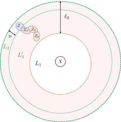
Figure 6: Subsets $Z$ and $\{Z_{1},Z_{2},\ldots,Z_{m^{\ast}}\}$ in Eq. (S.VIII.2.2) for $m^{\ast}=3$. The subset $Z$ is defined on the boundary region of $L_{2}^{\prime}=X[2\ell_{0}-2k]$, and hence $Z\subset L_{2}$ because of ${\rm diam}(Z)\leq 2k$. The other subsets $\{Z_{s}\}_{s=1}^{m^{\ast}}$ satisfy $Z_{1}\cap Z\neq\emptyset$, $Z_{2}\cap Z_{1}\neq\emptyset$ , $\ldots$, and $Z_{m^{\ast}}\cap Z_{m^{\ast}-1}\neq\emptyset$. The value of $m^{\ast}$ is taken so that $Z_{m^{\ast}}$ is included in the region $\tilde{L}=L_{2}\setminus L_{1}$, where the boson number is truncated.

S.VIII.2.2 Proof of Lemma 15

To estimate the upper bound of the norm (S.229), we use the standard recursive approach to prove the Lieb–Robinson bound [1, 5, 6]. We start with the following inequality [see Ineqs. (S.256 and S.284) in the supplementary material of Ref. [41]]:

$$\left\|[O_{Z}(\tilde{H}_{L^{\prime}_{2},\tau},x\to 0),\tilde{O}_{L_{1}}]\right\|\leq\mathcal{L}_{m^{\ast}},$$ (S.232)

where we choose $m^{\ast}$ such that $m^{\ast}\leq d_{Z,L_{1}}/(2k)$, and $\mathcal{L}_{m^{\ast}}$ is defined as

$$\mathcal{L}_{m^{\ast}}=2^{m^{\ast}+1}\|O_{Z}\|\cdot\|\tilde{O}_{L_{1}}\| \sum_{\begin{subarray}{c}Z_{1}\subset L^{\prime}_{2}\\ Z_{1}\cap Z\neq\emptyset\end{subarray}}\int_{0}^{x}\|\tilde{h}_{Z_{1},\tau_{1}}\|d\tau_{1}\sum_{\begin{subarray}{c}Z_{2}\subset L^{\prime}_{2}\\ Z_{2}\cap Z_{1}\neq\emptyset\end{subarray}}\int_{0}^{\tau_{1}}\|\tilde{h}_{Z_{2},\tau_{2}}\|d\tau_{2}$$

$$\cdots\sum_{\begin{subarray}{c}Z_{m^{\ast}}\subset L^{\prime}_{2}\\ Z_{m^{\ast}}\cap Z_{m^{\ast}-1}\neq\emptyset\end{subarray}}\int_{0}^{\tau_{m^{\ast}-1}}\|\tilde{h}_{Z_{m^{\ast}},\tau_{m^{\ast}}}\|d\tau_{m^{\ast}}.$$ (S.233)

Note that each of the interaction terms $\tilde{h}_{Z,\tau}$ ($Z\subset L^{\prime}_{2}$) is given in Eq. (S.214). Because of the condition $m^{\ast}\leq d_{Z,L_{1}}/(2k)$ and ${\rm diam}(Z)\leq 2k$, all the subsets $\{Z_{1},Z_{2},\ldots,Z_{m^{\ast}}\}$ in the above summations are included in the subsets $\tilde{L}$ (see also Fig. 6). Hence, we have

$$\sum_{\begin{subarray}{c}Z_{s}\subset L^{\prime}_{2}\\ Z_{s}\cap Z_{s-1}\neq\emptyset\end{subarray}}\|\tilde{h}_{Z_{s}}\|\leq\sum_{i\in Z_{s-1}}\sum_{\begin{subarray}{c}Z_{s}\subset L^{\prime}_{2}\\ Z_{s}:Z_{s}\ni i\end{subarray}}\|\tilde{h}_{Z_{s}}\|\leq\sum_{i\in Z_{s-1}}c_{3}\ell_{0}\leq c_{3}\gamma(2k)^{D}\ell_{0}$$ (S.234)

for $s=1,2,\ldots,m^{\ast}$, where we use Ineq. (S.VIII.2) and the inequality $|Z_{s-1}|\leq\gamma(2k)^{D}$ because of ${\rm diam}(Z_{s-1})\leq 2k$. We then obtain

$$\mathcal{L}_{m^{\ast}}\leq\frac{2[2xc_{3}\gamma(2k)^{D}\ell_{0}]^{m^{\ast}}}{m^{\ast}!}\|O_{Z}\|\cdot\|\tilde{O}_{L_{1}}\| \leq 2\zeta_{0}\left[\frac{2exc_{3}\gamma(2k)^{D}\ell_{0}}{m^{\ast}}\right]^{m^{\ast}}\|O_{Z}\|$$

$$=:2\zeta_{0}\left(\frac{xc_{3}^{\prime}\ell_{0}}{8km^{\ast}}\right)^{m^{\ast}}\|O_{Z}\|,$$ (S.235)

where we use $\|\tilde{O}_{L_{1}}\|=\zeta_{0}$ [see Eq. (S.89)], and $m^{\ast}!\geq(m^{\ast}/e)^{m^{\ast}}$. Note that we have defined $c_{3}^{\prime}=16ekc_{3}\gamma(2k)^{D}$ in the statement of Proposition 6.

Here, the distance $d_{Z,L_{1}}$ is larger than $\ell_{0}-4k$ because $Z\in\mathcal{S}_{L_{2}^{\prime}}$, and hence we obtain

$$m^{\ast}=\left\lfloor\frac{d_{Z,L_{1}}}{2k}\right\rfloor\geq\left\lfloor\frac{\ell_{0}-4k}{2k}\right\rfloor\geq\frac{\ell_{0}-6k}{2k}\geq\frac{\ell_{0}}{8k},$$ (S.236)

where we use the condition (S.85) in the last inequality. Using the above inequality for $m^{\ast}$ and the condition (S.231) for $x$, we have

$$\frac{xc_{3}^{\prime}\ell_{0}}{8km^{\ast}}\leq xc_{3}^{\prime}\leq e^{-1},$$ (S.237)

which reduces Ineq. (S.VIII.2.2) to

$$\mathcal{L}_{m^{\ast}}\leq 2\zeta_{0}\|O_{Z}\|e^{-m^{\ast}}\leq 2\zeta_{0}\|O_{Z}\|e^{-\frac{\ell_{0}}{2k}+3}.$$ (S.238)

By combining the above inequality with Eq. (S.232), we obtain the main inequality (S.230). This completes the proof. $\square$

[ End of Proof of Lemma 15]

Because $x\leq t\leq 1/(ec_{3}^{\prime})$, we use Lemma 15 to reduce the upper bound (S.228) to

$$\|\tilde{O}_{L_{1}}(\tilde{H}_{\tau},0\to t)-\tilde{O}_{L_{1}}(\tilde{H}_{L^{\prime}_{2},\tau},0\to t)\| \leq\sum_{Z:Z\in\mathcal{S}_{L^{\prime}_{2}}}\int_{0}^{t}2e^{3}\zeta_{0}\|\tilde{h}_{Z,x}\|e^{-\ell_{0}/(2k)}dx.$$ (S.239)

For an arbitrary site $i^{\prime}$ such that $i^{\prime}\in\partial L_{2}^{\prime}$, we have $i^{\prime}[2k]\subset\tilde{L}$, and hence we can use Ineq. (S.VIII.2) and obtain

$$\sum_{Z:Z\in\mathcal{S}_{L^{\prime}_{2}}}\|\tilde{h}_{Z,x}\|\leq\sum_{i^{\prime}\in\partial L_{2}^{\prime}}\sum_{Z\ni i^{\prime}}\|\tilde{h}_{Z,x}\|\leq\sum_{i^{\prime}\in\partial L_{2}^{\prime}}c_{3}\ell_{0}\leq c_{3}|\partial L_{2}^{\prime}|\ell_{0}.$$ (S.240)

We therefore reduce the upper bound (S.239) to

$$\|\tilde{O}_{L_{1}}(\tilde{H}_{\tau},0\to t)-\tilde{O}_{L_{1}}(\tilde{H}_{L^{\prime}_{2},\tau},0\to t)\|\leq 2e^{3}\zeta_{0}c_{3}t|\partial L_{2}^{\prime}|\ell_{0}e^{-\ell_{0}/(2k)}.$$ (S.241)

This completes the proof of Proposition 6. $\square$

S.IX Quench

S.IX.1 Setup of the quench dynamics

We consider the quench of the Hamiltonian from $H\to H^{\prime}$ with $H^{\prime}$ given by

$$H^{\prime}=H+h_{X_{0}}=H_{0}^{\prime}+V^{\prime},\quad X_{0}\subset i_{0}[r_{0}],$$ (S.242)

where $h_{X_{0}}$ is assumed to have the form of Eq. (S.9). In addition, $H_{0}^{\prime}$ and $V^{\prime}$ are the quenched Hamiltonians, which include free boson hopping and boson–boson interactions, respectively. We define the function $Q(q)$ as the upper bound of the norm of $h_{X_{0}}\bar{\Pi}_{X_{0},q}$:

$$\|h_{X_{0}}\bar{\Pi}_{X_{0},q}\|\leq Q(q),$$ (S.243)

where $\bar{\Pi}_{X_{0},q}$ has been defined in Eq. (S.79). The function $Q(q)$ characterizes the norm of the quench Hamiltonian when the boson number is truncated up to $q$. In Eq. (S.9), the boson–boson interactions can take arbitrary forms such as $e^{n_{i}n_{j}}$, but we assume here that $h_{X_{0}}$ includes only a finite-degree polynomial of the boson number operators, which also ensures that $Q(q)$ is given by a finite-degree polynomial [i.e., $Q(q)={\rm poly}(q)$].

S.IX.2 Main theorem

We assume that the initial state $\rho_{0}$ is a steady state under the Hamiltonian $H$. After the quench of the Hamiltonian, the state $\rho_{0}$ no longer satisfies $[\rho_{0},H^{\prime}]\neq 0$, and it evolves with time. Our purpose is to find the approximation error as

$$\left\|\rho_{0}(H^{\prime},t)-U_{i_{0}[R]}\rho_{0}U^{\dagger}_{i_{0}[R]}\right\|_{1},$$ (S.244)

where $U_{i_{0}[R]}$ is appropriately defined on the subset $i_{0}[R]$.

Intuitively, from Theorem 1, the quantity (S.244) is expected to obey the same upper bound as Eq. (S.20). However, the situation is not that simple. In considering $\rho_{0}(H^{\prime},t)$, we may consider

$$e^{-iH^{\prime}t}\rho_{0}=\mathcal{T}e^{-\int_{0}^{t}h_{X_{0}}(H,-x)dx}e^{-iHt}\rho_{0}=\mathcal{T}e^{-\int_{0}^{t}h_{X_{0}}(H,-x)dx}\rho_{0}e^{-iHt},$$ (S.245)

where we use $[\rho_{0},H]=0$ in the last equation. From Theorem 1, we can upper-bound

$$\left\|\left(h_{X_{0}}(H,-x)-U_{i_{0}[R]}h_{X_{0}}U^{\dagger}_{i_{0}[R]}\right)\rho_{0}\right\|_{1}.$$

To approximate $\mathcal{T}e^{-\int_{0}^{t}h_{X}(H,-x)dx}$, we need to consider

$$h_{X_{0}}(H,-t_{1})h_{X_{0}}(H,-t_{2})\cdots h_{X_{0}}(H,-t_{m})\rho_{0}$$ (S.246)

with $t_{1}\leq t_{2}\leq\cdots\leq t_{m}$. The approximation of $h_{X_{0}}(H,-t_{1})h_{X_{0}}(H,-t_{2})\cdots h_{X_{0}}(H,-t_{m})$ onto the region $i_{0}[R]$ is nontrivial only from Theorem 1. In addition, we need to consider that the norm of $h_{X_{0}}$ is not finitely bounded in general. In fact, we can address these problems and prove the following theorem.

Theorem 2.

Let $h_{X_{0}}$ be an arbitrary operator in the form of (S.9) that satisfies the condition (S.243). Then, for an arbitrary quantum state $\rho_{0}$ satisfying $[\rho_{0},H]=0$ and assuming that (1) holds, the time evolution $\rho_{0}(t)$ is approximated using the local unitary operator $U_{i_{0}[R]}$ supported on $i_{0}[R]$ with the following approximation error:

$$\left\|\rho_{0}(H^{\prime},t)-U_{i_{0}[R]}\rho_{0}U^{\dagger}_{i_{0}[R]}\right\|_{1}\leq\exp\left(c_{0}\bar{q}-C^{\prime}_{1}\frac{(R-r_{0})}{t\log(R)}+C^{\prime}_{2}\log(R)\right)\quad(t\geq 1),$$ (S.247)

where $C^{\prime}_{1}$ and $C^{\prime}_{2}$ are constants of $\mathcal{O}(1)$ which are independent of $\bar{q}$ and depend only on the details of the system. Moreover, the computation cost to construct the unitary operator $U_{i_{0}[R]}$ is at most

$$\exp\left[\mathcal{O}\left(R^{D}\log(R)\right)\right].$$ (S.248)

Remark. For $r_{0}=\mathcal{O}(1)$, $\bar{q}=\mathcal{O}(1)$, and $D=1$, in order to obtain a fixed error $\epsilon$, we need to choose $R$ as

$$R\approx t\log^{2}(t)+t\log(1/\epsilon)\log\log(1/\epsilon),$$ (S.249)

and hence the time complexity is given by

$$\exp\left[t\log^{3}(t)+t\log(1/\epsilon)\log\log^{2}(1/\epsilon)\right].$$ (S.250)

S.IX.3 Proof of Theorem 2

The proof is obtained using an approach similar to that used for Theorem 1. The approximation for the short-time evolution is crucial. We can prove the following proposition (see Sec. S.IX.4 for the proof).

Proposition 16.

Let $u_{X}$ be an arbitrary unitary operator such that $[u_{X},\hat{n}_{X}]=0$, $X\subseteq i[r]$, and $\Pi_{X,\geq q_{0}}u_{X}=0$ for fixed $q_{0}$. Then, the time evolution $\tilde{\rho}(H^{\prime},t)$ with

$$\tilde{\rho}:=u_{X}\rho_{0}u_{X}^{\dagger}$$ (S.251)

is approximated using a unitary operator $U_{X[\ell]}$ ($[U_{X[\ell]},\hat{n}_{X[\ell]}]=0$) as follows:

$$\left\|\tilde{\rho}(t)-U_{X[\ell]}\rho_{0}U_{X[\ell]}^{\dagger}\right\|_{1}\leq e^{c_{0}\bar{q}}e^{-\ell/\log(r)}$$ (S.252)

for $t\leq\Delta t_{0}$, where $\Delta t_{0}=\mathcal{O}(1)$, and the length $\ell$ is chosen such that it satisfies

$$\ell\geq C_{0}^{\prime}\log^{2}(r),$$ (S.253)

with $C_{0}^{\prime}=\mathcal{O}(1)$, which does not depend on $\bar{q}$. Moreover, the unitary operator $U_{X[\ell]}$ satisfies

$$U_{X[\ell]}\Pi_{X[\ell],\geq\max(q_{0},\eta^{\prime}\ell|X|/2)}=0$$ (S.254)

for $\eta^{\prime}=\mathcal{O}(1)$. In addition, the computational cost of preparing $U_{X[\ell]}$ is

$$\exp\left[\mathcal{O}\left((r+\ell)^{D}\log(r+\ell+q_{0})\right)\right].$$ (S.255)

From the above proposition, we can easily prove Theorem 2 by connecting the short-time evolution as described in Sec. S.IV.2. We adopt the same decomposition of the time and the length as in Sec. S.IV.2. First, we can derive an inequality similar to Eq. (S.48) as follows:

$$\left\|\rho_{0}(H^{\prime},t)-U_{X_{m_{t}}}^{(m_{t})}\rho_{0}U_{X_{m_{t}}}^{(m_{t})\dagger}\right\|_{1}\leq\sum_{m=0}^{m_{t}}\left\|\left(U_{X_{m-1}}^{(m-1)}\rho_{0}U_{X_{m-1}}^{(m-1)\dagger}\right)(H^{\prime},\Delta t)-U_{X_{m}}^{(m)}\rho_{0}U_{X_{m}}^{(m)\dagger}\right\|_{1},$$ (S.256)

where each of the unitary operators $\{U_{X_{m}}^{(m)}\}_{m=1}^{m_{t}}$ gives the approximation of

$$\left(U_{X_{m-1}}^{(m-1)}\rho_{0}U_{X_{m-1}}^{(m-1)\dagger}\right)(H^{\prime},\Delta t)\approx U_{X_{m}}^{(m)}\rho_{0}U_{X_{m}}^{(m)\dagger}.$$ (S.257)

By using Proposition 16 iteratively, we prove an inequality similar to Ineq. (S.IV.2):

$$\left\|\rho_{0}(H^{\prime},t)-U_{X_{m_{t}}}^{(m_{t})}\rho_{0}U_{X_{m_{t}}}^{(m_{t})\dagger}\right\|_{1}\leq\exp\left(c_{0}\bar{q}-\frac{\Delta t(R-r_{0})}{t\log(R)}+\frac{1}{\log(R)}+(C_{0}^{\prime}+1)\log(R)\right),$$ (S.258)

which reduces to the main inequality (S.247) by appropriately choosing $C_{1}^{\prime}$ and $C_{2}^{\prime}$. In addition, from Eq. (S.255), the construction of each operator $\{U_{X_{m}}^{(m)}\}_{m=1}^{m_{t}}$ has a maximum computational cost of

$$\exp\left[\mathcal{O}\left(R^{D}\log(R)\right)\right].$$ (S.259)

We thus prove Theorem 2. $\square$

S.IX.4 Proof of Proposition 16

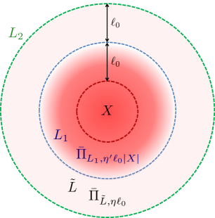
Figure 7: Boson number truncation. In the proof of Proposition 16, we truncate the boson number in the region $L_{1}$ in addition to that in $\tilde{L}$ [see Eq. (S.263)]. In the region $L_{1}$, the boson number distribution decays exponentially beyond $\mathcal{O}(|X|)$ [see Ineq. (S.262)].

We adopt the same definition of $\tilde{\rho}(H^{\prime},t)$ as in Eq. (S.64):

$$\tilde{\rho}(H^{\prime},t)=e^{-iH^{\prime}t}u_{X}\rho_{0}u_{X}^{\dagger}e^{iH^{\prime}t}.$$ (S.260)

Then, Proposition 3 and Corollary 4 hold for $\tilde{\rho}(H^{\prime},t)$ for $t\leq t_{0}$ because the quenched Hamiltonian has the form of Eq. (S.9).

In the second step, we also define the effective Hamiltonian by truncating the boson number in a particular region. Following Sec. S.V.2, we define the regions $L_{1}$, $L_{2}$, and $\tilde{L}$ in the same ways as in Eqs. (S.77) and (S.78). The main difference from the case of Subtheorem 1 is that we truncate the boson number on the subset $L_{1}$ in addition to the region $\tilde{L}$ (see Fig. 7). There are two main reasons for this additional truncation: i) we need to upper-bound the norm of $h_{X_{0}}$ ($X_{0}\in L_{1}$) in Eq. (S.242), and ii) to estimate the computational cost of constructing the unitary operator, we need to restrict the maximum boson number in the region $L_{1}$.

Here, we perform boson number truncation in the region $L_{2}$. In the region $L_{1}$, the bosons can become concentrated on one site, and hence we need to choose a sufficiently large truncation number. We note that the moment function $M^{(s)}_{i}(t)$ in the region $L_{1}$ can also be estimated by Proposition 3, which gives

$$M_{i}^{(s)}(t) \leq c^{\prime}_{1}e^{c_{0}\bar{q}}\zeta_{0}^{2}|X|^{3}(c_{1}s|X|)^{s}+c^{\prime\prime}_{1}e^{c_{0}\bar{q}}\zeta_{0}^{2}(c_{1}s)^{s}\quad(i\in L_{1}),$$ (S.261)

where we take $d_{i,X}=0$ in Ineq. (S.66). The above inequality yields

$$P_{i,\geq z_{0}}^{(t)}=e^{c_{0}\bar{q}-\mathcal{O}(z_{0}/|X|)}\quad(i\in L_{1})$$ (S.262)

if we use the Markov inequality.

We define the boson truncation operator $\bar{\Pi}_{L_{2},q,q^{\prime}}$ as follows:

$$\bar{\Pi}_{L_{2},q,q^{\prime}}:=\bar{\Pi}_{\tilde{L},q}\bar{\Pi}_{L_{1},q^{\prime}},$$ (S.263)

where $\bar{\Pi}_{L,q}$ has been defined in Eq. (S.79). Recall that $L_{2}=L_{1}\sqcup\tilde{L}$. By using this notation, we also define the effective Hamiltonian $\tilde{H}^{\prime}[L_{2},q,q^{\prime}]$ for the Hamiltonian $H^{\prime}$ in the same way as in Eq. (S.V.2).

To estimate the difference between the time evolutions by $H^{\prime}$ and $\tilde{H}^{\prime}[L_{2},q,q^{\prime}]$, we can use the proof technique we used for Proposition 5, which yields the following inequality:

$$\left\|\left[u_{X}(H^{\prime},-t)-u_{X}(\tilde{H}^{\prime}[L_{2},\eta\ell_{0},\eta^{\prime}\ell_{0}|X|],-t)\right]\rho_{0}(H^{\prime},t)\right\|_{1}\leq\frac{1}{8}e^{c_{0}\bar{q}}e^{-2\ell_{0}/\log(r)}$$ (S.264)

for $t\leq t_{0}$, where $\ell_{0}$ is chosen as in Eq. (S.83),

$$\ell_{0}\geq c_{2}\log^{2}(r),$$ (S.265)

and $\eta$ and $\eta^{\prime}$ are constants of $\mathcal{O}(1)$, which are chosen appropriately. In the following, for simplicity, we describe

$$\tilde{A}[L_{2},\eta\ell_{0},\eta^{\prime}\ell_{0}|X|]\to\tilde{A}\quad({\rm i.e.,}\ \tilde{H}^{\prime}[L_{2},\eta\ell_{0},\eta^{\prime}\ell_{0}|X|]\to\tilde{H}^{\prime})$$ (S.266)

for an arbitrary operator $A$ by omitting the information on the boson number truncation $[L_{2},\eta\ell_{0},\eta^{\prime}\ell_{0}|X|]$.

We focus on the time evolution of $\tilde{\rho}$ by $\tilde{H}^{\prime}$:

$$\tilde{\rho}(\tilde{H}^{\prime},t)=u_{X}(\tilde{H}^{\prime},-t)\rho_{0}(\tilde{H}^{\prime},t)[u_{X}(\tilde{H}^{\prime},-t)]^{\dagger}.$$ (S.267)

We first consider the local approximations of $u_{X}(\tilde{H}^{\prime},-t)$. For the unitary operator, we can prove the statement in Proposition 6, which gives

$$\left\|u_{X}(\tilde{H}^{\prime},-t)-U^{\dagger}_{1,L_{2}}u_{X}U_{1,L_{2}}\right\|\leq 2e^{3}c_{3}t|\partial L_{2}^{\prime}|\ell_{0}e^{-\ell_{0}/(2k)},$$

$$c_{3}:=4\bar{J}\eta\gamma(2k)^{D}d_{G},\quad c_{3}^{\prime}:=16ekc_{3}\gamma(2k)^{D}$$ (S.268)

for $t\leq 1/(ec_{3}^{\prime})$ with $[U_{1,L_{2}},\hat{n}_{L_{2}}]=0$, where we set $\zeta_{0}=1$ in Ineq. (S.94) because $\|u_{X}\|=1$. Note that the statement in Proposition 6 is not affected by the boson truncation on $L_{1}$, and hence Ineq. (S.IX.4) does not depend on $\eta^{\prime}$ (see also Sec. S.VIII). The unitary operator $U_{1,L_{2}}$ was given explicitly in Eq. (S.96) in Sec. S.V.3. Then, the unitary operator $U_{1,L_{2}}$ has the following form:

$$e^{-i\tilde{V}^{\prime}_{X[k]}t}\mathcal{T}e^{-i\int_{0}^{t}e^{i\tilde{V}^{\prime}\tau}\tilde{H}^{\prime}_{0,L_{2}^{\prime}}e^{-i\tilde{V}^{\prime}\tau}d\tau},$$ (S.269)

where $L_{2}^{\prime}:=X[2\ell_{0}-2k]$. When the above unitary operator acts on $u_{X}$ in Eq. (S.IX.4), it is equivalent to

$$e^{-i\tilde{V}^{\prime}_{L_{2}}t}\mathcal{T}e^{-i\int_{0}^{t}e^{i\tilde{V}^{\prime}_{L_{2}}\tau}\tilde{H}^{\prime}_{0,L_{2}^{\prime}}e^{-i\tilde{V}^{\prime}_{L_{2}}\tau}d\tau}=e^{-i(\tilde{H}^{\prime}_{0,L_{2}^{\prime}}+\tilde{V}^{\prime}_{L_{2}})t}=:U_{1,L_{2}}.$$ (S.270)

By combining Ineqs. (S.264) and (S.IX.4), we obtain

$$\left\|\left[u_{X}(H^{\prime},-t)-U^{\dagger}_{1,L_{2}}u_{X}U_{1,L_{2}}\right]\rho_{0}(H^{\prime},t)\right\|_{1}\leq\frac{1}{8}e^{c_{0}\bar{q}}e^{-2\ell_{0}/\log(r)}+2e^{3}c_{3}t|\partial L_{2}^{\prime}|\ell_{0}e^{-\ell_{0}/(2k)},$$ (S.271)

which yields

$$\left\|\tilde{\rho}(H^{\prime},t)-\left(U^{\dagger}_{1,L_{2}}u_{X}U_{1,L_{2}}\right)\rho_{0}(H^{\prime},t)\left(U^{\dagger}_{1,L_{2}}u_{X}U_{1,L_{2}}\right)^{\dagger}\right\|_{1}\leq\frac{1}{4}e^{c_{0}\bar{q}}e^{-2\ell_{0}/\log(r)}+4e^{3}c_{3}t|\partial L_{2}^{\prime}|\ell_{0}e^{-\ell_{0}/(2k)},$$ (S.272)

where we use the equation $\tilde{\rho}(H^{\prime},t)=u_{X}(H^{\prime},-t)\rho_{0}(H^{\prime},t)u_{X}(H^{\prime},-t)^{\dagger}$.

Here, the initial state $\rho_{0}$ is not invariant under the time evolution of $e^{-iH^{\prime}t}$. Therefore, the remaining task is to estimate the approximate error of

$$\rho_{0}(H^{\prime},t)\approx U_{2,L_{2}}\rho_{0}U_{2,L_{2}}^{\dagger},$$ (S.273)

where $U_{2,L_{2}}$ is appropriately chosen.

Lemma 17.

We can find a unitary operator $U_{2,L_{2}}$ that approximates $\rho_{0}(H^{\prime},t)$ with an error of

$$\left\|\rho_{0}(H^{\prime},t)-U_{2,L_{2}}\rho_{0}U_{2,L_{2}}^{\dagger}\right\|_{1}\leq\frac{1}{2}e^{c_{0}\bar{q}}e^{-2\ell_{0}/\log(r)}+4e^{3}Q(\eta^{\prime}\ell_{0}|X|)c_{3}t^{2}|\partial L_{2}^{\prime}|\ell_{0}e^{-\ell_{0}/(2k)},$$ (S.274)

where the function $Q(q)$ is given by Eq. (S.243).

S.IX.4.1 Proof of Lemma 17

We start with the equations

$$e^{-iH^{\prime}t}\rho_{0}=e^{-i\tilde{H}^{\prime}t}\rho_{0}+(e^{-iH^{\prime}t}-e^{-i\tilde{H}^{\prime}t})\rho_{0},$$ (S.275)

$$e^{-i\tilde{H}^{\prime}t}\rho_{0}=\mathcal{T}e^{-i\int_{0}^{\tau}\tilde{h}_{X_{0}}(\tilde{H},-\tau)}e^{-i\tilde{H}t}\rho_{0}$$

$$\quad\quad\quad\ \ =\mathcal{T}e^{-i\int_{0}^{\tau}\tilde{h}_{X_{0}}(\tilde{H},-\tau)d\tau}e^{-iHt}\rho_{0}-\mathcal{T}e^{-i\int_{0}^{\tau}\tilde{h}_{X_{0}}(\tilde{H},-\tau)d\tau}(e^{-i\tilde{H}t}-e^{-iHt})\rho_{0},$$ (S.276)

$$\mathcal{T}e^{-i\int_{0}^{\tau}\tilde{h}_{X_{0}}(\tilde{H},-\tau)d\tau}e^{-iHt}\rho_{0}$$

$$\quad\quad\quad\ \ =\mathcal{T}e^{-i\int_{0}^{\tau}u_{L_{2},\tau}^{\dagger}\tilde{h}_{X_{0}}u_{L_{2},\tau}d\tau}e^{-iHt}\rho_{0}+\left(\mathcal{T}e^{-i\int_{0}^{\tau}\tilde{h}_{X_{0}}(\tilde{H},-\tau)d\tau}-\mathcal{T}e^{-i\int_{0}^{\tau}u_{L_{2},\tau}^{\dagger}\tilde{h}_{X_{0}}u_{L_{2},\tau}d\tau}\right)e^{-iHt}\rho_{0},$$ (S.277)

where the unitary operators $u_{L_{2},\tau}$ in Eq. (S.277) are appropriately chosen. By combining the above equations, we can derive the following inequality:

$$\left\|e^{-iH^{\prime}t}\rho_{0}-\mathcal{T}e^{-i\int_{0}^{\tau}u_{L_{2},\tau}^{\dagger}\tilde{h}_{X_{0}}u_{L_{2},\tau}d\tau}e^{-iHt}\rho_{0}\right\|_{1}$$

$$\leq \left\|(e^{-iH^{\prime}t}-e^{-i\tilde{H}^{\prime}t})\rho_{0}\right\|_{1}+\left\|(e^{-i\tilde{H}t}-e^{-iHt})\rho_{0}\right\|_{1}+\left\|\left(\mathcal{T}e^{-i\int_{0}^{\tau}\tilde{h}_{X_{0}}(\tilde{H},-\tau)d\tau}-\mathcal{T}e^{-i\int_{0}^{\tau}u_{L_{2},\tau}^{\dagger}\tilde{h}_{X_{0}}u_{L_{2},\tau}d\tau}\right)\right\|.$$ (S.278)

The norms $\|(e^{-iH^{\prime}t}-e^{-i\tilde{H}^{\prime}t})\rho_{0}\|_{1}$ and $\|(e^{-i\tilde{H}t}-e^{-iHt})\rho_{0}\|_{1}$ can be derived by using the analyses that were used to obtain (S.VII.2.2). For the $\eta$ and $\eta^{\prime}$ chosen in Ineq. (S.264), we obtain the upper bound as

$$\left\|(e^{-iH^{\prime}t}-e^{-i\tilde{H}^{\prime}t})\rho_{0}\right\|_{1}\leq\frac{1}{8}e^{c_{0}\bar{q}}e^{-2\ell_{0}/\log(r)},\quad\left\|(e^{-i\tilde{H}t}-e^{-iHt})\rho_{0}\right\|_{1}\leq\frac{1}{8}e^{c_{0}\bar{q}}e^{-2\ell_{0}/\log(r)}.$$ (S.279)

Therefore, our task is to estimate the third term on the RHS of Ineq. (S.IX.4.1).

To this end, we use the following lemma.

Claim 18.

Let $A_{\tau}$ and $B_{\tau}$ be arbitrary time-dependent operators with continuous time dependence. Then, the difference between unitary operations by $A_{\tau}$ and $B_{\tau}$ is upper-bounded by

$$\|U_{A_{\tau},0\to t}-U_{B_{\tau},0\to t}\|\leq\int_{0}^{t}\|A_{\tau}-B_{\tau}\|d\tau$$ (S.280)

for arbitrary $t$, where we use the notation in Eq. (S.V.3).

Proof of Claim 18. For the proof, we first consider

$$U_{A_{\tau},0\to t+dt} =e^{-iA_{t+dt}dt}U_{A_{\tau},0\to t}+\mathcal{O}(dt^{2})$$

$$=e^{-iA_{t+dt}dt}U_{B_{\tau},0\to t}+e^{-iA_{t+dt}dt}\left(U_{A_{\tau},0\to t}-U_{B_{\tau},0\to t}\right)+\mathcal{O}(dt^{2})$$

$$=U_{B_{\tau},0\to t+dt}+\left(e^{-iA_{t+dt}dt}-e^{-iB_{t+dt}dt}\right)U_{B_{\tau},0\to t}+e^{-iA_{t+dt}dt}\left(U_{A_{\tau},0\to t}-U_{B_{\tau},0\to t}\right)+\mathcal{O}(dt^{2}).$$ (S.281)

Hence, if we define $\mathcal{G}(t):=\left\|U_{A_{\tau},0\to t}-U_{B_{\tau},0\to t}\right\|$, we have

$$\frac{d\mathcal{G}(t)}{dt}\leq\|A_{t}-B_{t}\|.$$ (S.282)

By integrating the above inequality, we obtain the main inequality (S.280). This completes the proof. $\square$

Using the above lemma, we obtain

$$\left\|\left(\mathcal{T}e^{-i\int_{0}^{t}\tilde{h}_{X_{0}}(\tilde{H},-\tau)d\tau}-\mathcal{T}e^{-i\int_{0}^{t}u_{L_{2},\tau}^{\dagger}\tilde{h}_{X_{0}}u_{L_{2},\tau}d\tau}\right)\right\|\leq\int_{0}^{t}\left\|\tilde{h}_{X_{0}}(\tilde{H},-\tau)-u_{L_{2},\tau}^{\dagger}\tilde{h}_{X_{0}}u_{L_{2},\tau}\right\|d\tau.$$ (S.283)

To approximate $\tilde{h}_{X_{0}}(\tilde{H},-\tau)$ by $u_{L_{2},\tau}^{\dagger}\tilde{h}_{X_{0}}u_{L_{2},\tau}$, we can use Proposition 6, which yields

$$\left\|\tilde{h}_{X_{0}}(\tilde{H},-\tau)-u_{L_{2},\tau}^{\dagger}\tilde{h}_{X_{0}}u_{L_{2},\tau}\right\|\leq 2e^{3}\|\tilde{h}_{X_{0}}\|c_{3}\tau|\partial L_{2}^{\prime}|\ell_{0}e^{-\ell_{0}/(2k)}.$$ (S.284)

Here, the unitary operator $u_{L_{2},\tau}$ is given by

$$u_{L_{2},\tau}=e^{i(\tilde{H}^{\prime}_{0,L_{2}^{\prime}}+\tilde{V}^{\prime}_{L_{2}})\tau},$$ (S.285)

where we follow the steps as in Eqs. (S.269) and (S.269). We therefore obtain

$$\left\|\left(\mathcal{T}e^{-i\int_{0}^{t}\tilde{h}_{X_{0}}(\tilde{H},-\tau)d\tau}-\mathcal{T}e^{-i\int_{0}^{t}u_{L_{2},\tau}^{\dagger}\tilde{h}_{X_{0}}u_{L_{2},\tau}d\tau}\right)\right\|\leq 2e^{3}\|\tilde{h}_{X_{0}}\|c_{3}t^{2}|\partial L_{2}^{\prime}|\ell_{0}e^{-\ell_{0}/(2k)}.$$ (S.286)

We choose $U_{2,L_{2}}$ as

$$U_{2,L_{2}}=\mathcal{T}e^{-i\int_{0}^{t}u_{L_{2},\tau}^{\dagger}\tilde{h}_{X_{0}}u_{L_{2},\tau}d\tau}.$$ (S.287)

By combining Ineqs. (S.279) and (S.286) with Ineq. (S.IX.4.1), we obtain

$$\left\|e^{-iH^{\prime}t}\rho_{0}-U_{2,L_{2}}e^{-iHt}\rho_{0}\right\|_{1}\leq\frac{1}{4}e^{c_{0}\bar{q}}e^{-2\ell_{0}/\log(r)}+2e^{3}\|\tilde{h}_{X_{0}}\|c_{3}t^{2}|\partial L_{2}^{\prime}|\ell_{0}e^{-\ell_{0}/(2k)}.$$ (S.288)

By explicitly writing $\|\tilde{h}_{X_{0}}\|$ without the simplified notation of Eq. (S.266), we obtain

$$\|\tilde{h}_{X_{0}}\|\to\|\tilde{h}_{X_{0}}[L_{2},\eta\ell_{0},\eta^{\prime}\ell_{0}|X|]\|=\|\tilde{h}_{X_{0}}\bar{\Pi}_{X_{0},\eta^{\prime}\ell_{0}|X|}\|\leq Q(\eta^{\prime}\ell_{0}|X|),$$ (S.289)

where we use Ineq. (S.243). Because of $e^{-iHt}\rho_{0}=\rho_{0}e^{-iHt}$, the above inequality reduces Ineq. (S.288) to the main inequality (S.274). This completes the proof. $\square$

[ End of Proof of Lemma 17]

By applying Ineq. (S.274) to Ineq. (S.272), we obtain

$$\left\|\tilde{\rho}(H^{\prime},t)-\left(U^{\dagger}_{1,L_{2}}u_{X}U_{1,L_{2}}\right)U_{2,L_{2}}\rho_{0}U_{2,L_{2}}^{\dagger}\left(U^{\dagger}_{1,L_{2}}u_{X}U_{1,L_{2}}\right)^{\dagger}\right\|_{1}$$

$$\leq\frac{3}{4}e^{c_{0}\bar{q}}e^{-2\ell_{0}/\log(r)}+4e^{3}c_{3}t(1+tQ(\eta^{\prime}\ell_{0}|X|))|\partial L_{2}^{\prime}|\ell_{0}e^{-\ell_{0}/(2k)}$$ (S.290)

for $t\leq 1/(ec_{3}^{\prime})$. Finally, we need to choose $C_{0}^{\prime}$ in the condition (S.253). Because $Q(q)$ is given by a finite-degree polynomial, the second term in the above inequality is roughly given by

$${\rm poly}(\ell_{0})\cdot{\rm poly}(r)e^{-\ell_{0}/(2k)},$$ (S.291)

where we use $X\subseteq i[r]$. Hence, we can find an $\mathcal{O}(1)$ constant $C_{0}^{\prime}$ such that for $\ell_{0}\geq(C_{0}^{\prime}/2)\log^{2}(r)$,

$$4e^{3}c_{3}t(1+tQ(\eta^{\prime}\ell_{0}|X|))|\partial L_{2}^{\prime}|\ell_{0}e^{-\ell_{0}/(2k)}\leq\frac{1}{4}e^{-2\ell_{0}/\log(r)}\leq\frac{1}{4}e^{c_{0}\bar{q}}e^{-2\ell_{0}/\log(r)}$$ (S.292)

holds. If we write

$$U_{X[2\ell_{0}]}:=U^{\dagger}_{1,L_{2}}u_{X}U_{1,L_{2}}U_{2,L_{2}},$$ (S.293)

Ineq. (S.IX.4.1) with Ineq. (S.292) gives the main inequality (S.252) with $\ell=2\ell_{0}$ and $\Delta t_{0}=1/(ec_{3}^{\prime})$. Note that we have defined $X[2\ell_{0}]=L_{2}$.

Finally, we consider the time complexity of preparing the unitary operator $U_{X[2\ell_{0}]}$. From Eqs. (S.270), (S.285), and (S.287), the unitary operator (S.293) is given by

$$U_{X[2\ell_{0}]}:=e^{i(\tilde{H}^{\prime}_{0,L_{2}^{\prime}}+\tilde{V}^{\prime}_{L_{2}})t}u_{X}e^{-i(\tilde{H}^{\prime}_{0,L_{2}^{\prime}}+\tilde{V}^{\prime}_{L_{2}})t}\mathcal{T}\exp\left[-i\int_{0}^{t}e^{i\left(\tilde{H}^{\prime}_{0,L_{2}^{\prime}}+\tilde{V}^{\prime}_{L_{2}}\right)\tau}\tilde{h}_{X_{0}}e^{-i\left(\tilde{H}^{\prime}_{0,L_{2}^{\prime}}+\tilde{V}^{\prime}_{L_{2}}\right)\tau}d\tau\right].$$ (S.294)

From this form and the initial condition $u_{X}\Pi_{X,\geq q_{0}}=0$ (see the statement in Proposition 16), we can immediately obtain the equation (S.254).

For any operator $O_{L_{2}}$ supported on $L_{2}$, after the boson number truncation $\bar{\Pi}_{L_{2},q,q^{\prime}}$, the number of parameters needed to describe $\bar{\Pi}_{L_{2},q,q^{\prime}}O_{L_{2}}\bar{\Pi}_{L_{2},q,q^{\prime}}$ is at most $[\max(q,q^{\prime})]^{|L_{2}|}$. To describe the initial unitary operator $u_{X}$, the number of parameters is less than $q_{0}^{|X|}$ because of the condition $\Pi_{X,\geq q_{0}}u_{X}=0$ in the statement. Now, we have $q=\eta\ell_{0}$ and $q^{\prime}=\eta^{\prime}\ell_{0}|X|$ as in Ineq. (S.264), and hence the time complexity of preparing $U_{X[2\ell_{0}]}$ is at most

$$\left[\max(q_{0},\eta^{\prime}\ell_{0}|X|)\right]^{\mathcal{O}(|L_{2}|)} =\exp\left[\mathcal{O}\left((r+\ell_{0})^{D}\log(r+\ell_{0}+q_{0})\right)\right]=\exp\left[\mathcal{O}\left((r+\ell)^{D}\log(r+\ell+q_{0})\right)\right]$$ (S.295)

for $\ell=2\ell_{0}$. This completes the proof of Proposition 16. $\square$