BigCarl: Mining frequent subnets from a single large Petri net

Abstract.

While there have been lots of work studying frequent subgraph mining, very few publications have discussed frequent subnet mining from more complicated data structures such as Petri nets. This paper studies frequent subnets mining from a single large Petri net. We follow the idea of transforming a Petri net in net graph form and to mine frequent sub-net graphs to avoid high complexity. Technically, we take a minimal traversal approach to produce a canonical label of the big net graph. We adapted the maximal independent embedding set approach to the net graph representation and proposed an incremental pattern growth (independent embedding set reduction) way for discovering frequent sub-net graphs from the single large net graph, which are finally transformed back to frequent subnets. Extensive performance studies made on a single large Petri net, which contains 10 K events, 40 K conditions and 30 K arcs, showed that our approach is correct and the complexity is reasonable.

1. Introduction

Frequent subgraph mining has been a hot research topic since the end of the last century (Jiang et al., 2013). However, before the discovery of the pattern growth approach, in particular the proposal of gSpan algorithm (Xifeng Yan and Jiawei Han, 2002), frequent subgraph mining was a very hard and tough task (Cook and Holder, 2007). This task became even more difficult when scientists tried to mine frequent subgraphs from a single large graph (Kuramochi, 2005). It invoked many research works (Kuramochi, 2005; Fiedler and Borgelt, 2007; Bringmann and Nijssen, 2008; Elseidy et al., 2014; Meng et al., 2020). The main difficulty is how to count the number of embedding copies of a frequent subgraph pattern in case that they are overlapped. To solve this problem, many techniques have been proposed. However, most of them have high computational complexity. For example, MIS (Kuramochi, 2005) and HO (Fiedler and Borgelt, 2007) are all NP-Hard. MNI (Elseidy et al., 2014) is polynomial, however, it is heuristic.

Besides that, another phenomenon has raised our attention. While there have been lots of work studying frequent subgraph mining, very few publications have discussed frequent subnet mining from more complicated data structures such as Petri nets (Reisig and Rozenberg, 1998; Murata, 1989). It was not until recently that a preprint has been published (Lu and Zhang, 2020), where frequent subnet mining from a set of Petri nets is studied.

The theory of Petri nets, or net theory for short, is a powerful theory for concurrent distributed systems (Yuan, 2013). It was founded by C.A. Petri in his seminal thesis ’Kommunikation mit Automaten’ in 1962 (Petri, 1962). Since then the net theory has experienced a rash development and found a wide scope of application, including machinery, chemistry, biology, linguistics, workflow analysis, and many others (Hu and Zhou, 2015; Liu et al., 2013; Khan et al., 2018; Silva, 2013; Smith, 2007; Peterson, 1981; Tax et al., 2018). Researches done in the past nearly 60 years have accumulated a huge repository of Petri net pieces. A deep analysis of this repository is needed. However, as we said above, we have found a serious lack of subnet mining study results. This situation has motivated us to do the research presented in the present paper, which studies frequent subnet mining from a single large Petri net.

Technically, we adopt the strategy of transforming a Petri net into net graph representation introduced in (Lu and Zhang, 2020) and doing frequent sub-net graph mining based on it, but with some modifications and extensions, which will be explained in section 2.2. To start sub-net graph mining, we first take a minimal traversal approach to produce a minimal DFS code of the net graph, which represents a canonical labeling of the net graph and is slightly different from (Lu and Zhang, 2020). The frequent sub-net graph mining is based on the maximal independent set support principle. The discovery procedure goes ahead in an incremental way. Finally, the discovered frequent sub-net graphs and their distinct embedding copies will be transformed back to Petri net form. At the end, extensive performance studies made on a single large Petri net, which contains 10 K events, 40 K conditions and 30 K arcs, showed that our approach is correct and the complexity is reasonable.

The remainder of the paper is arranged as follows: Section 2 presents the preliminaries of complete subnet and the net graph representation. Section 3 introduces the minimal traversal of a net graph. Section 4 explains the main idea of BigCarl algorithm under the maximal independent set support framework. Section  5 presents in detail the BigCarl algorithm Section 6 evaluates the net graph representation and BigCarl algorithm with a single large Petri net generated in a random way. Finally, section 7 provides some concluding remarks.

2. PRELIMINARY

2.1. Complete subnets

Petri nets differ from graphs not only in their topological structure (i.e., Petri nets have two types of nodes: the event nodes and the condition nodes) (Murata, 1989). According to the point of view of C.A.Petri himself, a subnet of a Petri net should be semantically complete (Peterson, 1977). This means if you cut off a subnet from a Petri net, then together with an event node, you should also cut off all its input and output condition nodes. This point of view plays an important role in defining frequent subnet mining. This paper extends the concept of complete subnets in (Lu and Zhang, 2020) by differentiating two types of complete subnets, where the e-type complete nets coincide with the complete nets defined in (Lu and Zhang, 2020).

Definition 0 (e-type/c-type complete subnet).

1. Given a Petri net $N$. If $e(c)$ is an event (condition) node of $N$, then $e(c)$ together with all its input and output conditions (events) is called an e-type (c-type) 1-complete subnet.
2. An e-type (c-type) m-complete subnet is composed by identifying some of the condition nodes (event nodes) of the m 1-complete subnets with each other.

$\hfill\square$

Our algorithm BigCarl mines only e-type frequent complete subnets. Since there are many different sorts of Petri nets, when we talk about Petri net in this paper, we always mean its basic sort: the pure C/E net, except if some special interpretation is given. Following is the definition.

Example 0.

Figure  1a borrows a Petri net from (Lu and Zhang, 2020),  1b and  1c show an e-type respectively c-type 1-complete subnet of  1a. Figure  1d and  1e show two different connections of  1b and  1c, where  1d is an e-type 2-complete subnet while  1e is a c-type 2-complete subnet.

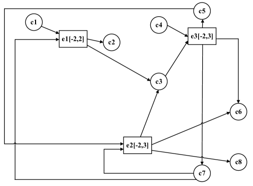
(a) A pure C/E net

(b) An e-type 1-complete subnet

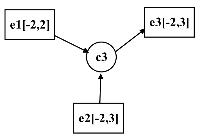
(c) A c-type 1-complete subnet

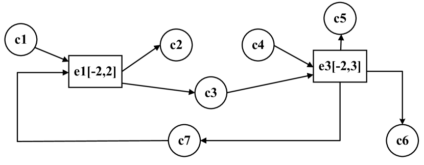
(d) An e-type 2-complete subnet composed by $e_{1}$ and $e_{3}$

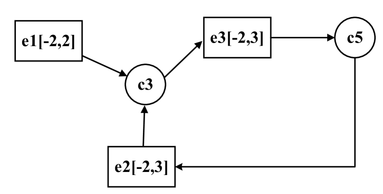
(e) A c-type 2-complete subnet composed by $c_{3}$ and $c_{5}$

Figure 1. A Petri net and its complete subnets

2.2. Net graph representation

Net graph is a graph-like representation introduced in (Lu and Zhang, 2020) for reducing the complexity of Petri nets’ frequent subnet mining. According to the e-type complete subnet and c-type complete subnet introduced above, we differentiate in this paper between two types of net graphs: the e-type and c-type net graphs.

Definition 0 (e-type net graph).

A e-type net graph $NGE=(V_{e},C_{e};W_{e})$ is a pseudo-graph transformed from a pure C/E net $N=(C,E;F)$, where
1. $V_{e}$ is the set of NGE’s nodes, $C_{e}=C$. $V_{e}=V+$tagging, where each $v\in V_{e}$ is represented as $e<$signed sequence of conditions connected to $e$ in $N$$>$ for some $e$ of $E$. Here $e$ plays the role of $v$’s node name. For any condition $c$ in this sequence, the sign is ’-’(’+’) if $F$ contains an arc from $c(e)$ to $e(c)$. Note that in this sequence, the signed conditions are alphabetically ordered where symbol ‘-’ is always before symbol ‘+’;
2. $W_{e}$ is the set of NGE’s edges. Each edge $w$ connecting $v_{1}$ and $v_{2}$ has a tagging which is a lexicographically ordered sequence (symbol ‘-’ is always before symbol ‘+’) of triples where each triple has the form $\{h_{1},c,h_{2}\}$, where $c$ is a condition of $C_{e}$ connecting the two nodes $e_{1}$ and $e_{2}$ of $E$, which are the node names of $v_{1}$ and $v_{2}$. ${h_{1}}=^{\prime}-^{\prime}(^{\prime}+^{\prime})$ means $F$ contains an arc from $c(e_{1})$ to $e_{1}(c)$. The same for ${h_{2}}$ and $e_{2}$.

$\hfill\square$

Definition 0 (c-type net graph).

A c-type net graph $NGC=(C_{c},E_{c};W_{c})$ is a pseudo-graph transformed from a pure C/E net $N=(C,E;F)$. All statements of definition  3 apply to $NGC$ if we exchange the roles of events and conditions.

$\hfill\square$

The following lemma shows that there is a dual relation between the two types of net graphs.

Lemma 0.

Given a C/E net $N$. Transform it to its dual form $N^{\prime}$ by renaming each event as a condition and each condition as an event while keeping the arcs unchanged. Construct $N$’s net graph $NG^{\prime}$. Transform $NG^{\prime}$ to its dual form $NG^{\prime\prime}$ by renaming each node as a condition and each condition in the node’s tagging and edge’s tagging as an event. At the same time reverse the signs in $G^{\prime}$’s tagging. Then $NG^{\prime\prime}$ is equal to $N$’s net graph $NG$.

Proof.

Omitted. ∎

Example 0.

Figure  2 shows the e-type net graph and c-type net graph transformed from the pure C/E net in figure  1a.

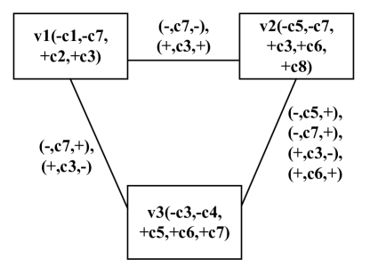
(a) An e-type net graph transformed from figure  1a

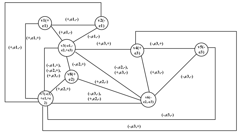
(b) A c-type net graph transformed from figure  1a

Figure 2. An e-type net graph and a c-type net graph

Lemma 0.

Given any pure C/E net $N$, there is a one-one transformation between $N$ and its e-type net graph representation and its c-type graph representation.

Proof.

Omitted. ∎

3. MINIMAL TRAVERSAL of a NET GRAPH

To start with frequent sub-net graph mining, similar to the idea of (Xifeng Yan and Jiawei Han, 2002), we first have to define a depth first traversal of the whole net graph which produces a canonical labeling of the net graph.. For that purpose, we need a lexicographic order of DFS codes. Following the idea of (Lu and Zhang, 2020), we do not sort the DFS codes in the lexicographic order after the algorithm has produced all DFS codes, but produce a minimal DFS code during a specific way of net graph traversal, the minimal traversal. However, the strategy taken in this paper is slightly different from that used in (Xifeng Yan and Jiawei Han, 2002). In order to assure the uniqueness of minimal traversal, we introduce a natural rule in the following for C/E net construction.

Definition 0 (clear C/E net).

A C/E net is called clear, if for any event node $e$,
1. No two of $e$’s input condition nodes have the same name, and
2. No two of $e$’s output condition nodes have the same name.

$\hfill\square$

This concept is semantically sound since it is meaningless to have repeated same condition nodes in an event node’s preset or postset. It can be generalized to other kinds of Petri nets. But for the moment we are only interested in C/E nets. We assume all C/E nets discussed in the remaining part of this paper are clear nets.

The following algorithm is a combination of gSpan’s idea about depth first travel and its idea about minimal traversal and our clear net definition above.

1

Input: $NGE$: e-type net graph

2 $i=0$;

3 Choose the minimal node $u$ (node with minimal tagging) as the starting of traversal;

Mark $u$ as current node and already visited, put $u$ in $MinE[0]$; // $MinE[0]$ is the set of all nodes of net graph with their taggings

4 while exist edges untraversed do

5       if backward edge $w_{1}$’s another node $v_{1}$ is minimal then

            put $w_{1}$ in $MinE[1]$, put $v_{1}$ in $MinE[0]$, make $v_{1}$ as current node; // $MinE[1]$ is the set of all 1-edges of net graph

6            

7      else

8            put minimal backward edge $w_{2}$(edge with minimal tagging) in $MinE[1]$;

9             put $w_{2}$’s another node $v_{2}$ in $MinE[0]$, make $v_{2}$ as current node;

10      $i=i+1$;

11       if there are untraversed forward edges from current node then

12            put minimal forward edge $w_{3}$ in $MinE[1]$, put $v_{3}$ in $MinE[0]$;

13             make $w_{3}$’s another node $v_{3}$ as current node, $i=i+1$;

14      

$NoE=i;$// $NoE$ is the id of edge when traversing

Algorithm 1 BigCarl-Minimal-DFS-Traversal ($NGE$: e-type net graph)

Lemma 0.

The decision of minima travel path in algorithm 1 is uniquely determined.

Proof.

For backwards traversal, the minimal node on the next ends of the backward edges is uniquely determined since all these end nodes have been traversed at least once and the least traverse number is uniquely determined. For forwards traversal, the forward edges must have different tagging since the conditions contained in the tagging of different forward edges must have different names according to the clear net principle. ∎

4. MAXIMUM INDEPENDENT SET SUPPORT

4.1. Subnet embedding overlap

For developing the BigCarl algorithm we first introduce two definitions about overlap.

Definition 0.

1. Two Petri nets have an e-type overlap if both sides have at least one event node in common or a c-type overlap if both sides have at least one condition node in common.
2. With the overlap concept introduced above, we can redefine m-complete subnets as follows: the connection of m e-type 1-complete subnets with help of c-type overlap is called an e-type m-complete subnet, while the connection of m c-type 1-complete subnets with help of e-type overlap is called a c-type m-complete subnet. The connect action itself is called e-connect respectively c-connect.

$\hfill\square$

Lemma 0.

Assume a pure C/E net $N$ is transformed to its e-type (c-type) net graph $NG$, where $N$’s e-type (c-type) complete nets $N_{1}^{\prime}$ and $N_{2}^{\prime}$ are transformed to two sub-net graphs $NG_{1}^{\prime}$ and $NG_{2}^{\prime}$. Then $N_{1}^{\prime}$ and $N_{2}^{\prime}$ do not have event (condition) node overlap if and only if $NG_{1}^{\prime}$ and $NG_{2}^{\prime}$ do not have node overlap.

Proof.

Straightforward. ∎

Our BigCarl algorithm adopts the MIS (Maximum Independent Set support) approach with a modification. While a standard MIS algorithm searches subgraph embedding without edge overlap, BigCarl searches subnet embedding without overlap of some node type. Due to semantic reason explained above, BigCarl either only mines e-type m-complete subnets, or only mines c-type m-complete subnets for any m. In the former case, c-type overlap is admitted as junction of several e-type 1-complete nets, while in the latter case, e-type overlap is admitted as junction of several c-type 1-complete nets. It can be proved that without such junctions frequent subnet mining would be incomplete.

4.2. Bulding a Maximum Independent Set

Definition 0 (level-k frequent sub-net graph).

Given a frequency threshold $MinSup>0$ and a net graph $NG$. $Ng^{\prime}$ is a connected sub-net graph. We call $Ng^{\prime}$ a frequent sub-net graph if $Ng^{\prime}$ has $k$ edges and if there are no less than $MinSup$ embedding copies in $NG$ which have no nodes in common.

$\hfill\square$

The discovery of frequent sub-net graphs is made in an incremental way. A level-k sub-net graph is one which contains k edges. Different from usual subgraph mining, a frequent level-0 sub-net graph is meaningful since it represents a 1-complete subnet (subnet with one event node and all condition nodes connected to it). Our algorithm BigCarl finds all level-0 frequent sub-net graphs with their maximal independent embedding set. BigCarl then tries to increase the frequent sub-net graphs level by level. In this process it keeps a maximal independent set of embedding for each candidate frequent sub-net graph. This set reduces gradually when the above pattern grows until the largest possible $k$ is reached.

We have also extended our approach to solve frequent subnet mining under c-type overlap and mixed e-c-type overlap. Note that although we just take the C/E net as an example model to study the problem of frequent subnet mining from a single large net, we have proved that this approach applies also to a large set of different Petri net classes.

5. BIGCARL ALGORITHM

The BigCarl algorithm mines frequent subnets from a single large Petri net. A Petri net will be first transformed into an e-type net graph introduced above, on which the subnet mining is done. In this section we only discuss e-type subnet mining. The technique of C-type subnet mining is similar.

1

2

Output: The set of frequent net graphs and their embeddings

3

1 Sort the code units in both $MinE[0]$ and $MinE[1]$ according to their alphabetical order;

2 Remove infrequent nodes from $MinE[0]$ and put the patterns of the remaining nodes (frequent level-0 net graphs) in $MinF[0]$, such that the nodes in $MinE[0,j]$ are the embedding of the $j$-th node pattern in $MinF[0]$;

3 Remove infrequent edges from $MinE[1]$ and put the patterns of the remaining edges (frequent level-1 net graphs) in $MinF[1]$, such that the edges in $MinE[1,j]$ are the embedding of the $j$-th edge pattern in $MinF[1]$;

Call Algorithm Finding all frequent sub-net graphs (1, $MinF[1],MinE[1],\emptyset,MinF[1],MinE[1],MinSup$);

Algorithm 2 Mining frequent sub-net graphs ($MinSup$)

In the following algorithm, we use a queue $MinFC[k]$ to save the $k$ candidate patterns in a net graph (Line 1). All the embedding copies of these candidate patterns are saved in a hash-map $MinFEC[k,j]$ (Line 2). If two embedding occur in the same $S[h]$, which means they have the condition overlap phenomenon, then an overlap graph can be constructed. Each embedding in the hash-map $MinFEC[k,j]$ is the node, each condition overlap relationship is the edge (Line 3-4). If the maximum independent set support is no less than the frequency threshold $MinSup$, use a queue $MinF[k]$ to save the frequent sub-net graphs of the level-$k$ (Line 5-10). Line 11-21 show the generating procedure of level-$k$ frequent net graph in a level-wise manner. In line 14, for each frequent 1-edge in net graph, add it into the level-$k$ frequent sub-net graph to form the level-(k+1)-candidate sub-net graph. In line 20, an early stop filtering rule is said that if there exist level-$(k+1)$ frequent sub-net graphs, the edges of embedding should no less than $(k+1)\times MinSup$.

1

2

1

2for $j=1$ to $|MinFC[k]|$ do

       // $|MinFC[k]|$ is the number of candidate level-k patterns

3       for $m=1$ to $|MinFEC[k,j]|$ do

             // $|MinFEC[k,j]|$ is the number of candidate embedding copies of the j-th level-k pattern

4             put the $m$-th embedding $e(m)$ in all $S[h]$ whenever $e(m)$ contains the $h$-th node of the net graph;

5             construct an overlap graph with all embedding in $MinFEC[k,j]$ as nodes and add an edge between ant two nodes if they appear in the same $S[h]$;

6             Call the find largest independent set algorithm to get an independent node set;

7             if its size is no less than $MinSup$ then

8                   put the $j$-th pattern of $MinFC[k]$ in $MinF[k]$;

9                   put the independent node set in $MinFE[k,j]$;

10            

11      

1312$i=0$;

1514 if $MinF[k]\not=\emptyset$ then

17      16 for $j=1$ to $|MinF[k]|$ do

19            18foreach pattern $p(1)$ for $MinF[1]$ which can be connected to the $j$-th level-$k$ pattern to form a candidate level-$(k+1)$ pattern $p(k+1)$ do

20                  

22                  21$i=i+1$;

24                  23 if no less than $MinSup$ level-$k$ embedding copies in $MinFE[k,j]$ can be extended with an embedding of $p$ from $MinFE[1]$ then

26                        25put these embedding copies in $MinFEC[k+1,i]$;

28                        27 remove all other embedding copies from $S$;

29                        

31                        30put $p(k+1)$ in $MinFC[k+1]$;

32                  

33            

34      

3635if $(k+1)\times MinSup\leq NoE$ then

38      37Call Algorithm Finding all frequent sub-net graphs ($k+1$, $MinFC[k+1],MinFEC[k+1],S,MinF[1],MinFE[1],MinSup$);

39

Algorithm 3 Finding all frequent sub-net graphs ($k,MinFC[k],MinFEC[k],S,MinF[1],MinFE[1],MinSup$)

6. EXPERIMENTAL EVALUATION

6.1. A methdology for generating big C/E net

Since large-scale C/E net resources are not available, the test nets ware generated in a random way. To verify the correctness and efficiency of BigCarl, we have designed a naïve algorithm, called DigCarl, which runs directly on the pure C/E net itself. The results show that the frequent sub-net graphs and subnets obtained by two algorithms are consistent. Our BigCarl algorithm outperforms the DigCarl approach largely. We implemented these two algorithms in C++. All the experiments are conducted on a PC with Intel (R) Core (TM) i7-6700 CPU@3.40HZ and 32G RAM, and the operating system is Windows 10.

Definition 0 (BIG C/E net).

A basic C/E net consists of an event node with some input/output condition nodes connected to it.

$\hfill\square$

The following algorithms extend the Petri net generation functions of (Lu and Zhang, 2020).

1

2Input a large (small) positive integer $U$ as the maximum of event nodes if a large (small) net has to be generated;

3 Input a large (small) positive integer $H$ as the maximum of arcs connecting events with conditions if a dense (sparse) net has to be generated;

4 Input $x=0(x=1)$ if a c-type (e-type) overlap is to be used when connecting two C/E nets;

5 Create a first basic C/E net;

Call algorithm 5 $U$ times, each time generate a basic C/E net connecting the existing net with at most $H$ arcs by using the x-type overlap approach.

Algorithm 4 Generate an experimental C/E net ($x,U,H$)

1

2if $x=0(1)$ then

3       connect net $N_{1}$ with $N_{2}$ with at most $H$ random c-type (e-type) node overlaps;

Algorithm 5 connect$(x,H,N_{1},N_{2})$

In the above algorithms, a large net is generated as target of frequent subnet mining. The generated small nets will be inserted in the large net to test the BigCarl algorithm. Only c-type overlap is used for net connection, which plays also a role in frequent net graphs embedding processing of algorithm 2-3. However, when small nets are inserted (embedded) in a large net, both types of overlap are used. Since algorithms 2-3 only care e-overlap of embedding, we have included e-type overlap in algorithm 4-5 just for showing that frequent subnet mining with e-type overlap is also possible.

Example 0.

Reconsider Figure  1 in a reverse way as a net generation process. Then 1b (1c) is an e-type (c-type) basic net. 1d(1e)is a net connection with c-type(e-type)overlap.

6.2. Testing with planted nets

Inspired by the planted motif approaches in frequent subgraph mining (Yang et al., 2009), we design a planting strategy to test the correctness of BigCarl. First, we use the following terminology: (1) Planting net. The c-connect (e-connect) copies are generated based on these nets. (2) Big Planted net. The net where the copies are already planted in. (3) Big_net. The incremental net that is waiting for the connection of big planted nets. The details are depicted as follows.

1

Input: A set of planting nets $NS$, two parameters $g,H$, which denote the maximum of events in each planted net and the maximum of arcs connected with each event, the frequency threshold $0<Minsup<N$;

2 Call algorithm 4 to generate a test net under $g,H$ constraints;

3 foreach planting net $s\in NS$ do

4      Generate two random integers $c(s),e(s)$ such that $Minsup<c(s)\leq N,Minsup<e(s)\leq N$;

5       Generate $c(s)$ c-connect copies of $s$ randomly, and put them into $S$;

6       Generate $e(s)$ e-connect copies of $s$ randomly, and put them into $S$;

7Shuffle $S$;

// disorder all the copies randomly

8 foreach selected disordered copy $y\in S$ do

9      Call connect $(0,x,y)$ or connect $(1,x,y)$ to produce a big test net $x[+]y$;

Algorithm 6 Planting-nets($NS,g,H,MinSup$)

The validation rule is that for each big planted big nets in $NS$, perform BigCarl algorithm and check whether the mined results contain the planting net $s$ and their copies or not. The detail can be illustrated as algorithm 7. The testing result be can seen in table 1.

1

1 Given $m$ copies of a small net $N^{\prime}$ where the size of each small net is no less than $m$;

// make sure the enough overlap

2 Randomly generate $n$ pairs of natural numbers (denoting pairs of small net copies) where each natural number is between 1 and $m(m-1)$;

3 Insert the $m$ copies of $N^{\prime}$ in $N$ one by one;

4 When the $j$-th copy is inserted, it must have a c-overlap with each $h$-th copy for $h<j$;

// The $h$-th copy is inserted in $N$ earlier than $j$-th copy does

5 Check whether $(h,j)$ is a pair generated above;

// This means they should have a c-overlap

Algorithm 7 Generate frequent subnet in a single large net with predefined overlap graph

Example 0.

Suppose the initial test net has 3K nodes, 6K edges. We use the small net which has 100 nodes, 200 edges to generate the copies. Let $MinSup=50$, suppose each small net has $m=10(m<MinSup)$ copies.

Table 1. The procedure of building overlap graph and calculate the maximum independent set

level-k	#Embedding	Edges in overlap graph	Maximal independent set	Runtime (s)
1	780	187	410	1820
2	408	100	280	890
3	276	56	172	265
4	115	27	67	87
5	41	10	23	38

6.3. Performance of BigCarl

In this section, we will verify the results with two experiments. (1) The reduction power of net graph structures. When the number of arcs increasing, the ratio of net graph edges’ number/ big C/E net arcs’ number reduces exponentially. (2) The scalability of BigCarl vs. DigCarl.

6.3.1. The reduction power of net graph structures

Under the same parameters of net generating, we generate 5 big C/E nets with a different scale. We investigate the change of the ratio (e-type net graph edges’ number/big C/E net arcs’ number) by increasing the number of nodes in big C/E nets (10K,28K,58K,162K,490K, including events, conditions) and increasing the number of arcs as shown in Table 2. The reduction ratio can be seen in table 2 and figure 3.

Table 2. The edges number of e-type net graph vs. the arcs number of big C/E nets

#arcs in big C/E nets (AB)	5400	11,518	23,416	64,811	281,575
#edges in e-type net graph (AE)	1522	3196	4699	6971	25420
AE/AB	28%	27.7%	20%	10.7%	9%

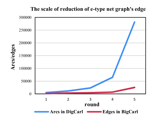
Figure 3. The reduction of e-type net graph’s edge

6.3.2. The scalability of BigCarl vs. DigCarl

The following experiments compare the salability of BigCarl with DigCarl by evaluating (1) the runtime (in seconds), (2) the memory overheads (in MB) depending on the growing number of big C/E net arcs. Note that due to the hardware limitations, the big C/E nets (with almost 10K nodes, 20K edges) cannot be mined in a tolerable time. Therefore, we mainly focus on the big C/E nets with maximum 5K nodes and 10K edges to compare the scalability. Suppose the frequency threshold is 10, varying the number of nodes (2835, 4163, 4927,5561,6019) and the number of arcs (6K,7K,8K,9K,10K). The trend of runtime and memory usage can be seen in figure 4a and 4b. It shows that the overheads of BigCarl are significantly reduced compared with those of DigCarl. Figure 4a shows that the growth trend of both BigCarl and DigCarl is exponential, whereas DigCarl has been running for more than 1 day (it cannot be shown in the figure).

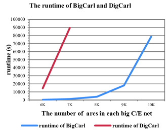
(a) Runtime

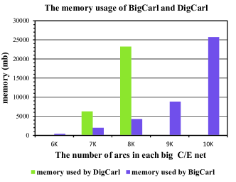
(b) Memory

Figure 4. The comparison of BigCarl and DigCarl

7. CONCLUSION

The main contributions of this paper can be summarized as follows: This paper is the first one addressing the problem of finding frequent subnets from a single large Petri net. We not only make use of Petri net’s basic properties in algorithm design but have extended them with a duality principle about Petri nets’ event and condition nodes. With this principle we differentiate between c-type and e-type (net graph, overlap, connection, basic net, complete net, frequent subnet mining) and thus expanded the application possibility of our research results largely. We established a detailed framework for implementing the MIS algorithm in case of Petri nets and their net graph representation. To evaluate the effectiveness of our approach we developed a technique of frequent subnet mining under predefined overlap graph. This technique inserts copies of small Petri nets in a large Petri net with randomly generated overlap schema. This technique provides the possibility of checking the correctness of frequent subnet mining. Our BigCarl algorithm can mine 10K nodes scale Petri nets transform 100K nodes scale Petri nets in net graphs.

References

- (1)
- Agrawal et al. (1993) Rakesh Agrawal, Tomasz Imieliński, and Arun Swami. 1993. Mining Association Rules Between Sets of Items in Large Databases. SIGMOD Rec. 22, 2 (June 1993), 207–216. https://doi.org/10.1145/170036.170072
- Bringmann and Nijssen (2008) Björn Bringmann and Siegfried Nijssen. 2008. What Is Frequent in a Single Graph? In Advances in Knowledge Discovery and Data Mining, Takashi Washio, Einoshin Suzuki, Kai Ming Ting, and Akihiro Inokuchi (Eds.). Vol. 5012. Springer Berlin Heidelberg, Berlin, Heidelberg, 858–863. https://doi.org/10.1007/978-3-540-68125-0_84 Series Title: Lecture Notes in Computer Science.
- Cook and Holder (2007) Diane J. Cook and Lawrence B. Holder (Eds.). 2007. Mining graph data. Wiley-Interscience, Hoboken, N.J. OCLC: ocm67361258.
- Elseidy et al. (2014) Mohammed Elseidy, Ehab Abdelhamid, Spiros Skiadopoulos, and Panos Kalnis. 2014. GraMi: Frequent Subgraph and Pattern Mining in a Single Large Graph. Proc. VLDB Endow. 7, 7 (March 2014), 517–528. https://doi.org/10.14778/2732286.2732289
- Fiedler and Borgelt (2007) Mathias Fiedler and Christian Borgelt. 2007. Support Computation for Mining Frequent Subgraphs in a Single Graph. (2007), 6.
- Hu and Zhou (2015) H. Hu and M. Zhou. 2015. A Petri Net-Based Discrete-Event Control of Automated Manufacturing Systems With Assembly Operations. IEEE Transactions on Control Systems Technology 23, 2 (March 2015), 513–524. https://doi.org/10.1109/TCST.2014.2342664
- Jiang et al. (2013) Chuntao Jiang, Frans Coenen, and Michele Zito. 2013. A survey of frequent subgraph mining algorithms. The Knowledge Engineering Review 28, 1 (March 2013), 75–105. https://doi.org/10.1017/S0269888912000331
- Khan et al. (2018) Yasir Imtiaz Khan, Alexandros Konios, and Nicolas Guelfi. 2018. A Survey of Petri Nets Slicing. ACM Computing Surveys (CSUR) 51, 5 (Dec. 2018), 109. https://doi.org/10.1145/3241736
- Kuramochi (2005) Michihiro Kuramochi. 2005. Finding Frequent Patterns in a Large Sparse Graph*. Data Mining and Knowledge Discovery 11, 3 (Nov. 2005), 243–271. https://doi.org/10.1007/s10618-005-0003-9
- Liu et al. (2013) G. Y. Liu, Z. W. Li, Kamel Barkaoui, and Abdulrahman M. Al-Ahmari. 2013. Robustness of deadlock control for a class of Petri nets with unreliable resources. Information Sciences 235, 6 (2013), 259–279.
- Lu and Zhang (2020) Ruqian Lu and Shuhan Zhang. 2020. PSpan: Mining Frequent Subnets of Petri Nets. ArXiv and Journal of Computational Sciences. (2020).
- Meng et al. (2020) Jinghan Meng, Napath Pitaksirianan, and Yi-Cheng Tu. 2020. Counting frequent patterns in large labeled graphs: a hypergraph-based approach. Data Mining and Knowledge Discovery 34, 4 (July 2020), 980–1021. https://doi.org/10.1007/s10618-020-00686-9
- Murata (1989) T. Murata. 1989. Petri nets: Properties, analysis and applications. Proc. IEEE 77, 4 (April 1989), 541–580. https://doi.org/10.1109/5.24143
- Peterson (1977) James L. Peterson. 1977. Petri nets. ACM Computing Surveys (CSUR) 9, 3 (1977), 223–252. ISBN: 0360-0300 Publisher: ACM New York, NY, USA.
- Peterson (1981) James Lyle Peterson. 1981. Petri Net Theory and the Modeling of Systems. Prentice Hall PTR, Upper Saddle River, NJ, USA.
- Petri (1962) Carl Adam Petri. 1962. Kommunikation mit Automaten. Ph.D. Dissertation.
- Reisig and Rozenberg (1998) Wolfgang Reisig and Grzegorz Rozenberg. 1998. Lectures on Petri Nets I: Basic Models: Advances in Petri Nets. Springer Science & Business Media. Google-Books-ID: 4BbFfLMZqnYC.
- Silva (2013) Manuel Silva. 2013. Half a century after Carl Adam Petri’s Ph.D. thesis: A perspective on the field. Annual Reviews in Control 37, 2 (Dec. 2013), 191–219. https://doi.org/10.1016/j.arcontrol.2013.09.001
- Smith (2007) Connie U. Smith. 2007. Introduction to Software Performance Engineering: Origins and Outstanding Problems. In Formal Methods for Performance Evaluation, Marco Bernardo and Jane Hillston (Eds.). Vol. 4486. Springer Berlin Heidelberg, Berlin, Heidelberg, 395–428. https://doi.org/10.1007/978-3-540-72522-0_10
- Tax et al. (2018) Niek Tax, Natalia Sidorova, Wil M. P. van der Aalst, and Reinder Haakma. 2018. LocalProcessModelDiscovery: Bringing Petri Nets to the Pattern Mining World. In Application and Theory of Petri Nets and Concurrency (Lecture Notes in Computer Science), Victor Khomenko and Olivier H. Roux (Eds.). Springer International Publishing, Cham, 374–384. https://doi.org/10.1007/978-3-319-91268-4_20
- Xifeng Yan and Jiawei Han (2002) Xifeng Yan and Jiawei Han. 2002. gSpan: graph-based substructure pattern mining. In 2002 IEEE International Conference on Data Mining, 2002. Proceedings. IEEE Comput. Soc, Maebashi City, Japan, 721–724. https://doi.org/10.1109/ICDM.2002.1184038
- Yang et al. (2009) Tianbao Yang, Rong Jin, Yun Chi, and Shenghuo Zhu. 2009. Combining link and content for community detection: a discriminative approach. In Proceedings of the 15th ACM SIGKDD international conference on Knowledge discovery and data mining - KDD ’09. ACM Press, Paris, France, 927. https://doi.org/10.1145/1557019.1557120
- Yuan (2013) Chong-Yi Yuan. 2013. Application of Petri Nets. SCIENCE PRESS, Beijing, China.