Fixation and Fluctuations in Two-Species Cooperation

Abstract

Cooperative interactions pervade in a broad range of many-body populations, such as ecological communities, social organizations, and economic webs. We investigate the dynamics of a population of two equivalent species A and B that are driven by cooperative and symmetric interactions between these species. For an isolated population, we determine the probability to reach fixation, where only one species remains, as a function of the initial concentrations of the two species, as well as the time to reach fixation. The latter scales exponentially with the population size. When members of each species migrate into the population at rate $\lambda$ and replace a randomly selected individual, surprisingly rich dynamics ensues. Ostensibly, the population reaches a steady state, but the steady-state population distribution undergoes a unimodal to trimodal transition as the migration rate decreases below a critical value $\lambda_{c}$. In the low-migration regime, $\lambda<\lambda_{c}$, the steady state is not truly steady, but instead strongly fluctuates between near-fixation states, where the population consists of mostly A’s or of mostly B’s. The characteristic time scale of these fluctuations diverges as $\lambda^{-1}$. Thus in spite of the cooperative interaction, a typical snapshot of the population will contain almost all A’s or almost all B’s.

1 Introduction

Competitive interactions have played a prominent role in the literature of ecological and evolutionary dynamics, as well as in economics and sociology [1, 2, 3]. Resource limitations and their impact in defining the outcome of competition among species has shaped a large part of evolutionary thinking. A counterpoint to competition is cooperativity in which there are positive interactions and feedback loops between species. These mechanisms have received increasing attention recently [4, 5]. In fact, it is the presence of cooperative interactions, where positive reciprocal exchanges are at work, that appear to drive innovations in evolution and also maintain biodiversity in Nature [5].

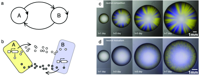
Figure 1: In pairwise cooperation (a) the replication (closed arrows) of a given species A requires the help of B and vice versa. This feedback occurs, for example, when two types of bacteria A and B each lack a metabolite for reproduction that is supplied by the other species (small circles in (b)). Such cooperative feedbacks are commonplace and help maintaining diversity. Experimental set-ups using engineered bacteria (c-d) reveal the marked difference between competitive and cooperative interactions. In (c), two equal competitors grow on a Petri dish and locally exclude each other, as shown by the growing bands that indicate the presence of only one strain. With cooperativity (d), the mutual dependency drives both strains to persist and mix.

Cooperation, or mutualism, has been part of mathematical models of populations since the formulation of Lotka-Volterra equations [2] and a variety of statistical physics models of human cooperation [6, 7]. In its most abstract form, two species (for example, $A$ and $B$ in Fig. 1(a)) “help” each other by means of a mutual positive interaction; in some cases, both partners completely rely on one another for survival. This feature underlies the two-species system in Fig. 1(b), where a given species requires the other to replicate because each species needs a molecule that is produced by the partner species.

Recent experimental studies have shown that such cooperative populations can in fact be engineered. By following the scheme in Fig. 1(b), it is possible to create a completely symmetric pairwise dependence and make these mixed populations grow on a Petri dish [8, 9, 10]. Figure 1(c) shows the outcome of symmetric competition when each strain is marked with a different fluorescent protein: each strain locally out competes the other, thereby generating stripes of segregated domains. The cooperatively interacting population, on the other hand, constrains both species to remain in proximity, leading to a well-mixed population (Fig. 1(d)). These simple engineered, or synthetic, bacterial populations, which can be tuned so that they become virtually symmetric, allow one to explore the fundamental dynamical features of interacting living consortia and also study the impact of stochasticity [11, 12, 13].

In this paper, we present an analytic approach to understand the role of stochasticity in a simple two-species stochastic model of cooperation. This model represents a special case of evolutionary game dynamics [14, 15, 16, 17], with a specific and particularly simple form of the payoff matrix. We emphasize that we are not treating a general ecological model, but rather a simplified system in which only cooperative interactions occur. This scenario appears to be more relevant for the microbiome [18, 19, 20]. Current advances in microbial ecology involve experimental setups with a small number of interacting species [21, 22]. In this model, we treat both closed and open populations, in which there is either no migration or a finite rate of migration into the population, respectively. We define microscopic rules that incorporate both cooperativity, in which each species helps the other, as well as neutrality, in which neither species is preferred over the other. We first determine the steady state of the population in the absence of stochastic fluctuations. For a finite population, we then incorporate stochasticity and determine the time until fixation is reached for the situation where no migration can occur. When migration is allowed (with compensatory removal), the population now reaches a steady state; however, the character of this steady state dramatically changes as function of the migration rate. For large migration rate, both species are present in roughly equal abundances. However, for a sufficiently small migration rate, the population strongly fluctuates between consisting of nearly all A or all B. Thus a typical realization of the population has a completely different character that the average population. This change in behavior is mirrored by a bimodal to trimodal transition in the shape of the steady-state probability distribution of species abundances.

In Sec. 2, we outline basic features of our two-species cooperation model in the absence of migration. We solve the model in the mean-field approximation and then include the role of stochasticity due to the finiteness of the population. For a finite population, we determine the fixation probability as a function of the initial population composition and the time until fixation, where only a single species remains. In Sec. 5, we incorporate migratory inflow, with compensatory removal, so that the population size remains fixed and reaches a steady state. We discuss basic features of this steady state, including the intriguing feature that the species abundances can exhibit huge fluctuations, even though time-averaged properties are constant. We give some concluding remarks in Sec. 6

2 Two-species cooperation

We investigate a finite population of $N$ particles, with $n$ of species A and $N-n$ of species B. The population undergoes repeated reaction events in which each event consists of the following steps (Fig. 2):

1. Pick a random pair of particles.

2. If the pair is AB, one member of this pair reproduces; if the pair is AA or BB, nothing happens.

3. The newly reproduced offspring replaces one randomly selected particle in the remainder of the population.

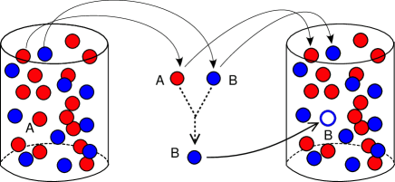
Figure 2: The reaction step in two-species cooperation. Two randomly selected particles happen to be from different species, namely A and B (red and blue). One of them reproduces (B, blue), an event that is aided by the presence of the other (A, red). The offspring replaces another randomly selected particle from the remainder of the population. In the example shown, the newly generated B replaces an A.

Thus interactions between members of different species are cooperative in nature, while members of the same species are non interacting. The replacement step (iii) ensures that the total population remains fixed. The lack of interactions between AA and BB pairs follows from the assumption of strict mutualism, i.e., replication occurs if and only if both species are present (as sketched in Fig. 2). After each update, time is incremented by $\frac{1}{N}$. This time increment corresponds to each particle undergoing, on average, steps (i)–(iii) in a single time unit. While this dynamics manifestly conserves the total number of particles, the composition of the population can change. When the population consists entirely of a single species—either all A’s or all B’s—there is no further dynamics and the population fixates.

If an A reproduces in a single interaction, then with probability $1-\frac{n}{N}\equiv 1-x$, the A offspring replaces a B and $n\to n+1$. Conversely, with probability $x=\frac{n}{N}$, the A offspring replaces an existing A so that $n$ does not change. The probability $a_{n}$ at which $n\to n+1$ therefore is

$$a_{n}=2x(1-x)\times\tfrac{1}{2}\times(1-x)=x(1-x)^{2}\,.$$ (1a)

Throughout, we use the variables $$n x=\frac{n}{N} 2x(1-x) \frac{1}{2} 1-x n\to n-1$$ and interchangeably. In (1a), the factor gives the probability a randomly selected pair is AB, the factor gives the probability that the A in this pair reproduces, and the factor gives the probability that the A offspring replaces a B. By the same reasoning, when a B reproduces in an interaction, the probability at which is

$$b_{n}=2x(1-x)\times\tfrac{1}{2}\times x=x^{2}(1-x)\,.$$ (1b)

Here the trailing factor $$x$$ in (1b) accounts for the probability that the B offspring replaces an A. Finally, the probability that the number of A’s and B’s does not change is given by

$$x^{2}+(1-x)^{2}+2x(1-x)\big{[}\tfrac{1}{2}x+\tfrac{1}{2}(1-x)\big{]}=1-x(1-x)=1-a_{n}-b_{n}\,.$$ (1c)

The terms $x^{2}+(1-x)^{2}$ give the probability to pick either an AA or BB pair, for which no change in $n$ occurs. For the last term, $2x(1-x)$ is again the probability of picking an AB pair, while the factor in the square brackets is the probability that the offspring (either A or B with probability $\frac{1}{2}$) replaces its own kind so that $n$ does not change.

3 Mean-Field Approaches

3.1 Rate Equation

Using the probabilities in Eqs. (1), the rate equation for the average number of A’s is

$$\dot{n}=N\left(a_{n}-b_{n}\right)=Nx(1-x)(1-2x)\,,$$ (2a)

or equivalently,

$$\dot{x}=x(1-x)(1-2x)\,.$$ (2b)

To keep the notation simple, $n$ and $x$ refer to average values in this section; that is, we do not write angle brackets. This rate equation has a stable fixed point at $x=\frac{1}{2}$ and unstable fixed points at $x=0$ and $x=1$. The stability of the fixed point at $x=\frac{1}{2}$ arises because the transition probabilities (1) tend to reduce population imbalances. Thus the steady state in this continuum description is a static population that consists of equal densities of A’s and B’s. That is, cooperativity promotes diversity in the mean-field description.

The solution to the rate equation (2b) may be straightforwardly obtained by first performing a partial fraction decomposition:

$$dt=\frac{dx}{x(1-x)(1-2x)}=dx\left(\frac{1}{x}-\frac{1}{1-x}+\frac{4}{1-2x}\right)\,,$$

from which

$$t =\int_{x_{0}}^{x}dy\left(\frac{1}{y}-\frac{1}{1-y}+\frac{4}{1-2y}\right)=-4\ln\frac{x(1-x)(1-2x)}{x_{0}(1-x_{0})(1-2x_{0})}\,.$$

We then obtain $x(t)$ by solving the resulting cubic equation. For $t\to\infty$, the limiting behavior is

$$x(t)\simeq\frac{1}{2}-2\,x_{0}(1-x_{0})(1-2x_{0})\,e^{-t/4}\,,$$ (3)

so that the stable fixed point $x^{*}=\frac{1}{2}$ is approached exponentially quickly in time.

3.2 Master Equation and Its Moments

In the stochastic dynamics where $n$ is a discrete variable, the true fixed points are at $x=0$ and $x=1$. Even though the fixed point at $x^{*}=\frac{1}{2}$ is stable in the continuum limit, stochastic fluctuations allow the population to explore the full state space and eventually get trapped at either $x=0$ or $x=1$. This behavior is analogous to the extinction phenomena that arise, for example, in the logistic birth-death process, $A\to 2A$ and $2A\to 0$, as well as other reactions of this genre [23, 24, 25, 26]. In these reactions, the rate equation predicts a steady population, $N_{\rm s}$, which is determined by the balance between the birth and death rates. However, in the true stochastic dynamics, the population fluctuates around $N_{\rm s}$, which actually is the quasi steady-state value. Ultimately, a sufficiently large fluctuation occurs that leads to extinction, from which there can be no escape, with an extinction time that scales exponentially in $N_{\rm s}$ [23, 24, 25, 26, 27].

To understand the stochastic dynamics for two-species cooperation, we study $P_{n}(t)$, the probability that the population consists of $n$ A’s and $(N-n)$ B’s at time $t$. The time dependence of this probability distribution is given by

$$\dot{P}_{n} =N\Big{[}a_{n-1}P_{n-1}+b_{n+1}P_{n+1}-\big{(}a_{n}+b_{n}\big{)}P_{n}\Big{]}\,.$$ (4)

When the number of particles $N$ is small, the set of equations (4) can be straightforwardly solved. For the initial condition of equal numbers of A’s and B’s, both $P_{0}(t)$ and $P_{N}(t)$ approach $\frac{1}{2}$ as $t\to\infty$, while all the other $P_{n}(t)$ vanish exponentially quickly in time. This direct approach quickly becomes tedious as $N$ increases, however, and to gain insight into the long-time dynamics for general $N$, it is useful to study low-order moments of $P_{n}$. From Eq. (4) and using $a_{n}$ and $b_{n}$ from Eqs. (1), the first moment obeys

$$\langle\dot{x}\rangle=\frac{1}{N}\sum_{n}n\dot{P}_{n} =\sum_{1\leq n\leq N}\left\{n\,a_{n-1}P_{n-1}+n\,b_{n+1}P_{n+1}-n\,\big{(}a_{n}+b_{n})P_{n}\right\}$$

$$=\sum_{1\leq n\leq N}\left\{(n+1)\,a_{n}P_{n}+(n-1)\,b_{n}P_{n}-n\,\big{(}a_{n}+b_{n}\big{)}P_{n}\right\}$$

$$=\sum_{1\leq n\leq N}(a_{n}-b_{n})P_{n}=\big{\langle}x(1-x)(1-2x)\big{\rangle}\,.$$ (5a)

Here we now explicitly write angle brackets to denote average values. Under the assumption of no correlations, that is, $$\langle x^{k}\rangle=\langle x\rangle^{k}$$, (5) reproduces the rate equation (2b).

Similarly, the equation of motion for the second moment is

$$\langle\dot{x}^{2}\rangle=\frac{1}{N^{2}}\sum_{n}n^{2}\dot{P}_{n} =\frac{1}{N}\sum_{1\leq n\leq N}\left\{n^{2}a_{n-1}P_{n-1}+n^{2}\,b_{n+1}P_{n+1}-n^{2}\,\big{(}a_{n}+b_{n}\big{)}P_{n}\right\}$$

$$=\frac{1}{N}\sum_{1\leq n\leq N}\left\{(n+1)^{2}\,a_{n}P_{n}+(n-1)^{2}\,b_{n}P_{n}-n^{2}\,\big{(}a_{n}+b_{n}\big{)}P_{n}\right\}$$

$$=\frac{1}{N}\langle x(1-x)\rangle+2\langle x^{2}(1-x)(1-2x)\rangle\,.$$ (5b)

It is more convenient to express (5) and (3.2) in terms of $z\equiv 2x-1$, which lies in the range $[-1,1]$. Doing so, we obtain

$$\begin{split}\langle\dot{z}\rangle&=-\tfrac{1}{2}\langle z(1-z^{2})\rangle\\ \langle\dot{z}^{2}\rangle&=\big{\langle}(1-z^{2})\big{(}\tfrac{1}{N}-z^{2})\big{\rangle}\,,\end{split}$$ (6)

which are both symmetric about $z=0$. If we make the assumption of no correlations, that is, $\langle z^{k}\rangle=\langle z\rangle^{k}$, then the first equation reproduces the result that $z=0$ is a stable fixed point. The second equation then predicts that the width of the distribution initially grows and eventually “sticks” at the value $\sqrt{N}$. To check this point, we numerically integrated Eqs. (4) for small values of $N$. From the resulting solution, we find that the width of the probability distribution initially grows with time and later approaches a nearly fixed value that is proportional to $\sqrt{N}$. However, at very long times, there is slow leakage of the probability distribution to the true stochastic fixed points at $z=\pm 1$. Thus the probability distribution eventually approaches two delta-function peaks at these fixed points. This behavior cannot be captured by low-order moment equations, such as (6). Instead, we need to study the full stochastic dynamics; this is done in the following section.

4 Fixation Probability and Fixation Time

We now turn to two quantities of primary interest in the stochastic dynamics, namely, (i) the fixation (or exit) probability $E_{n}$, and (ii) the fixation time $T_{n}$. The fixation probability $E_{n}$ is defined as the probability that a population of size $N$ that initially contains $n$ particles of type A reaches the static fixation state of all A’s. We use the backward Kolmogorov equation [28, 29] to compute the fixation probability. In this approach, $E_{n}$ satisfies the recursion

$$E_{n}=a_{n}E_{n+1}+b_{n}E_{n-1}+\big{(}1-a_{n}-b_{n}\big{)}E_{n}\,.$$ (7)

Since the process renews itself after each event, we can express the fixation probability from the state that contains $n$ A’s in terms of the appropriately weighted average of the fixation probabilities after a single step to the states $n-1$, $n$, and $n+1$. The weights are merely the hopping probabilities to these respective states. Equation (7) is subject to the boundary conditions $E_{0}=0$ and $E_{N}=1$. The first condition corresponds to the impossibility of reaching a population of all A’s if the initial state contains no A’s, while the second condition corresponds to the initial state coinciding with the desired final state of all A’s

The solution to (7) is (see A for the calculational details)

$$E_{n}=\sum_{m=0}^{n-1}\left[\binom{N-1}{m}\right]^{-1}\,\Big{/}\sum_{m=0}^{N-1}\left[\binom{N-1}{m}\right]^{-1}\,.$$ (8)

Neither of these sums has a closed form, but for $N\to\infty$ the denominator approaches 2 [30]. For $N\gg 1$, $E_{n}$ and its continuum counterpart $E(x)$ (see also A) are nearly independent of $x=\frac{n}{N}$ when $x$ is not close to 0 or 1. Figure 3 shows this dependence of $E_{n}$ on $n$. Also shown are the corresponding results from discrete simulations of the fixation process. Simulations are carried out by setting a finite size ($N$) array of particles with two possible states. Each iteration the particles interact following rules (ii) and (iii) with the interaction rates given by expressions (1a) and (1b). Time is updated by $\Delta t=\left[N\left(a_{n}+b_{n}\right)\right]^{-1}$ after each iteration.

The anti-sigmoidal shape of $E_{n}$ arises from the underlying drift that tends to drive any initial population towards $x=\frac{1}{2}$. Eventually, a large and rare stochastic fluctuation causes the population to escape this effective potential well and reach fixation. This anti-sigmoidal shape also strongly contrasts with the Moran process [31], which is symmetric (neutral), but non-cooperative. Here an AB pair equiprobably converts to either AA or to BB. As a result of this lack of cooperativity, the fixation probability in the strictly neutral Moran process is simply the linear function $E(x)=x$ [31, 32, 33, 29].

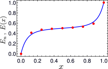
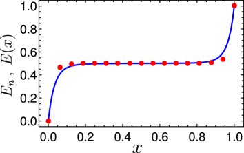
Figure 3: Dependence of the discrete and continuum fixation probabilities, $E_{n}$ and $E(x)$, versus $x$ for the cases $N=8$ and 16. The smooth curves represent $E(x)$ from Eq. (30) and the dots represent simulation results.

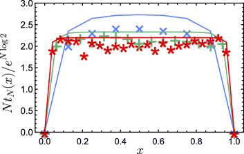
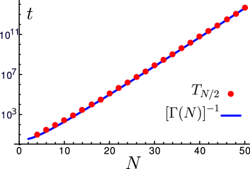
Figure 4: (a) Dependence of the fixation time $T_{n}$ versus $x=\frac{n}{N}$ using a data-collapse scheme by resetting the scale $T_{n}\to Ne^{-N\log 2}T_{n}$ for each $N$ value. This scaling factor corresponds to the prediction made in Eq. (16). The solid lines follow the predictions obtained from Eq. (10). The plot marks {$\times$, + and $*$} correspond to simulated average fixation times for $N=8,\ 16$ and $24$ in blue, green and red colors, respectively. Each data point is obtained by averaging $10^{3}$ simulated fixation processes at corresponding values of $n$ and $N$. (b) Dependence of the fixation time from the symmetric initial state, $T_{N/2}$ (red dots) computed by (10) and the WKB prediction for the inverse leakage rate from the quasi-steady state (blue line), following (16).

We now investigate the fixation time $T_{n}$, which is defined as the average time for the population of $N$ particles to first reach either of the two fixation states, $n=0$ or $n=N$, when the population initially contains $n$ A’s. Within the same backward Kolmogorov framework as that used for the fixation probability, the fixation time satisfies [28, 29]

$$T_{n} =a_{n}T_{n+1}+b_{n}T_{n-1}+\big{(}1-a_{n}-b_{n}\big{)}T_{n}+\delta t\,.$$ (9)

Again $T_{n}$ may be expressed as the appropriately weighted average of the fixation time after a single hopping event to the states $n-1$, $n$, and $n+1$, plus the time $\delta t=\frac{1}{N}$ required for this single step. The latter corresponds to each particle being updated once, on average, in a single time unit. The equation for $T_{n}$ is subject to the boundary conditions $T_{0}=T_{N}=0$; namely, if the population starts in a fixation state, the time to reach this state is 0. The result for the fixation time is (see B)

$$T_{n}=E_{n}\sum_{m=1}^{N-1}Q_{m}-\sum_{m=1}^{n-1}Q_{m}\,,$$ (10)

where

$$Q_{n}\equiv\alpha_{n}+r_{n}\,\alpha_{n-1}+r_{n}\,r_{n-1}\,\alpha_{n-2}+\cdots+r_{n}\,r_{n-1}\cdots r_{2}\,\alpha_{1}\,,$$

with $Q_{0}=0$, $r_{n}=b_{n}/a_{n}$, and $\alpha_{n}\equiv\delta t/a_{n}$.

It does not seem possible to reduce (10) to a compact form, but the main feature of this exact expression is that the fixation time scales exponentially in $N$ and is nearly independent of $n$ (or, equivalently, $x$), except for $n$ close to 0 or to $N$ (Fig. 4). The exponential dependence on $N$ again arises because of the existence of an effective potential well, whose depth grows linearly with $N$, which draws the population toward the state $x=\frac{1}{2}$. The near independence of the fixation time on the initial condition is a consequence of the population being drawn toward the bottom of this potential well, where the concentrations of A and B are equal. As a result, the value of the fixation time for any initial value of $x$ is close to the fixation time when the population starts from the bottom of the potential well at $x=\frac{1}{2}$.

It is possible, however, to obtain an analytical expression for the average fixation time by the WKB method [23, 24, 25, 26]. The idea of this approach is that the probability distribution settles into a quasi-steady state that assumes an exponential large-deviation form. From Eq. (4), there is a slow leakage from this quasi-steady state to the fixation state whose rate, $\Gamma(N)$, is given by

$$\Gamma(N)\,\delta t=b_{1}\widetilde{P}_{1}+a_{N-1}\widetilde{P}_{N-1}=2b_{1}\widetilde{P}_{1}\ ,$$ (11)

i.e., the flux from states that are one step away from fixation to the fixation states. Here the tilde denotes the steady-state distribution and we also use the symmetry $n\leftrightarrow N-n$. We then identify the inverse of this leakage rate with the fixation time.

We obtain an approximate equation for the continuum probability distribution $\widetilde{P}_{n}\to\widetilde{P}(x)$ by setting the time derivative in the master equation (4) to zero, and writing $n\pm 1$ as $x\pm\delta x$ to give

$$a(x-\delta x)\widetilde{P}(x\!-\!\delta x)+b(x+\delta x)\widetilde{P}(x\!+\!\delta x)=\left[a(x)+b(x)\right]\widetilde{P}(x)\ .$$ (12)

We now assume that $\widetilde{P}(x)$ has the exponential form $\widetilde{P}(x)\sim e^{S(x)/\delta x}=e^{NS_{0}(x)+S_{1}(x)+\cdots}$ and substitute this form into (12) to give (up to $O(1)$)

$$S_{0}(x)=\int^{x}dz\log\left[\frac{a(z)}{b(z)}\right]\ ,\quad S_{1}(x)=-\frac{1}{2}\log\left[a(x)b(x)\right]\,.$$ (13)

Now using (1a) and (1b) for $a(x)$ and $b(x)$, we have

$$\tilde{P}(x)\sim\frac{e^{NS_{0}(x)}}{x^{3/2}(1-x)^{3/2}}\ ,$$ (14)

with $S_{0}(x)=-x\log x-(1-x)\log(1-x)$. Note that the action $S_{0}(x)$ is peaked at the quasi-state state $x=\frac{1}{2}$. We normalize $\widetilde{P}(x)$ by using the Laplace method for $N\to\infty$ [34],

$$\int^{1}_{0}\frac{e^{NS_{0}(x)}}{x^{3/2}(1-x)^{3/2}}\,dx\approx\sqrt{\frac{32}{N}}\;e^{N\log 2}\ ,$$

so that

$$\widetilde{P}(x)\simeq\frac{N}{\sqrt{32\pi}}\;\frac{e^{N\left[-x\log x-(1-x)\log(1-x)-\log 2\right]}}{x^{3/2}(1-x)^{3/2}}\ .$$ (15)

We now compute the fixation rate $\Gamma$ by substituting

$$\widetilde{P}\big{(}\tfrac{1}{N}\big{)}\simeq\frac{N^{3}}{\sqrt{32\pi}}\;e^{1-N\log 2}\quad\text{and}\quad b\big{(}\tfrac{1}{N}\big{)}\simeq\frac{1}{N^{2}}\,,$$

into Eq. (11) to give

$$\Gamma(N)=\frac{Ne}{\sqrt{8\pi}}\;e^{-N\log 2}\ .$$ (16)

We now identify the inverse of this rate with the average fixation time. As shown in Fig. 4(b), this inverse rate accurately matches the simulation data for the fixation time.

5 Two-species cooperation with migration

We now incorporate migration into the dynamics, in which particles of either species migrate into the population at the same fixed rate $\lambda$, and each new particle replaces a randomly selected existing particle. Because migration is accompanied by replacement, the population size remains fixed, which is the physically most relevant case. Now the population is driven to a steady state rather than to fixation and we want to understand the nature of this steady state.

5.1 Probability Distribution

For a population that consists of $n$ A’s and $(N-n)$ B’s, suppose that the migrant is an A. With probability $\frac{1}{2}(1-x)$, the A migrant replaces a B and $n\to n+1$, while with probability $\frac{1}{2}x$, the A migrant replaces an A, and the composition of the population remains the same. Similar reasoning applies when the migrant is a B. As a result of a migration event, the average change in the number of A’s is $\frac{1}{2}(1-x)-\frac{1}{2}x$. The rate equation for $n$ now is (compare with Eq. (2))

$$\langle\dot{n}\rangle=N(1-\lambda)\left[x(1-x)(1-2x)\right]+\tfrac{1}{2}N\lambda(1-2x)\,.$$ (17)

For $\lambda>0$, $x=0$ and $x=1$ are no longer fixed points and only the remaining fixed point at $x=\frac{1}{2}$ is stable. In the absence of fluctuations, the population is thus driven to a steady-state distribution, $P_{n}(t\to\infty)$, that is peaked about $x=\frac{1}{2}$. Because there is no absorbing state in the stochastic dynamics, we might anticipate a similar behavior for $P_{n}(t\to\infty)$ when stochasticity is accounted for. We will show, however, that within the Fokker-Planck approximation the steady-state distribution can either be unimodal or trimodal in shape and the latter case corresponds to a steady state that is not truly steady.

The probability distribution $P_{n}$ is now governed by the master equation

$$\dot{P}_{n} =N(1-\lambda)\left[a_{n-1}P_{n-1}+b_{n+1}P_{n+1}-\big{(}a_{n}+b_{n}\big{)}P_{n}\right]$$

$$\qquad\qquad+N\lambda\left[c_{n-1}P_{n-1}+d_{n+1}P_{n+1}-\big{(}c_{n}+d_{n}\big{)}P_{n}\right]\,,$$ (18)

with hopping probabilities due to migration that are given by

$$c_{n}=\frac{1}{2}\left(1-\frac{n}{N}\right)\qquad\qquad d_{n}=\frac{1}{2}\frac{n}{N}\,.$$ (19)

We now determine the continuum probability distribution in the Fokker-Planck approximation. As we shall see, this continuum expression for the probability distribution matches simulation data quite well, thus justifying the Fokker-Planck approximation ex post facto as a way to probe steady-state properties.

In terms of $x=\frac{n}{N}$, $dx=\frac{1}{N}$, $P_{n}\to P(x)$, we expand (5.1) in a Taylor series up to second order. This gives the Fokker-Planck equation [35, 28]

$$P_{t} =-\Big{\{}\!(1\!-\!2x)\left[(1\!-\!\lambda)\,x(1\!-\!x)+\tfrac{\lambda}{2}\right]P(x,t)\!\Big{\}}_{x}+\frac{1}{2N}\Big{\{}\!\left[(1\!-\!\lambda)\,x(1\!-\!x)+\tfrac{\lambda}{2}\right]P(x,t)\!\Big{\}}_{xx}$$

$$\equiv-\big{\{}v(x)\,P(x,t)\big{\}}_{x}+\big{\{}D(x)\,P(x,t)\big{\}}_{xx}\,,$$ (20)

where the subscripts denote partial derivatives.

The steady state is defined by solving this equation with the left-hand side set to zero. Integrating once gives $(DP)_{x}-vP=B$, where $B$ is a constant. We determine the constant by evaluating this equation at the symmetry point $x=\frac{1}{2}$. Because the probability distribution is symmetric about $x=\frac{1}{2}$, $P_{x}(x\!=\!\frac{1}{2})=0$. Moreover, at $x=\frac{1}{2}$, $v=0$ and $D_{x}=0$, which implies that $B=0$. Thus we only need to solve $(DP)_{x}-vP=0$, whose solution is

$$P(x) =C\,\exp\bigg{\{}\int^{x}dy\,\,\frac{v(y)-D_{y}(y)}{D(y)}\bigg{\}}=C\,\exp\bigg{\{}-\log D(x)+\int^{x}dy\,\,\frac{v(y)}{D(y)}\bigg{\}}$$

$$=\frac{C}{D(x)}\;\exp\bigg{\{}\int^{x}dy\,\,2N(1-2y)\bigg{\}}$$

$$=C^{\prime}\,\left[\frac{1}{(1\!-\!\lambda)x(1\!-\!x)+\frac{\lambda}{2}}\right]\,\,e^{2Nx(1-x)}\,,$$ (21)

where the constant $C^{\prime}$ is determined by normalization.

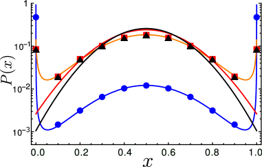
Figure 5: Steady-state probability distributions for $N=10$ on a semi-logarithmic scale for values of $\lambda/\lambda_{c}=10^{-4},10^{-2},10^{0}\ \text{and}\ 10^{1}$ in blue, orange, red and black, respectively. The respective data points correspond to simulation results.

For $\lambda\to 0$, $P(x)$ is concentrated near $x=0$ and near $x=1$; these peaks correspond to the near-fixation states. Because of rare fluctuations, however, the population stochastically switches between states where almost all particles are of type A to states where almost all particles are of type B. Naively, one therefore anticipates that the steady-state distribution should be bimodal, with a peak at each of the two near-fixation states. Unexpectedly, there always remains a peak at $x=\frac{1}{2}$ (which may be vanishingly small), so that the this distribution is trimodal in the small-$\lambda$ regime. As $\lambda$ increases beyond a critical value, the steady-state distribution undergoes a trimodal to unimodal transition (Fig. 5).

For fixed $N$, we determine the transition between trimodality and unimodality by finding the point(s) where $P^{\prime}(x)=0$. This calculation gives, after straightforward algebra,

$$P^{\prime}(x)\propto(1-2x)\,\,e^{2Nx(1-x)}\,\,\left[2N-\frac{(\lambda-1)}{D(x)^{2}}\right]\,,$$

where again $D(x)$ is the diffusion coefficient defined by Eq. (5.1). The leading factor of $1-2x$ equals 0 at $x=\frac{1}{2}$ and corresponds to the extremum in the distribution at $x=\frac{1}{2}$.

However, there are additional extrema at the points where the factor in the square brackets equals 0. To determine these extrema, we first determine the zero of this factor at $x=0,1$. Thus we have the condition $2N=(1-\lambda)/(\lambda/2)^{2}$. Since we will find that $\lambda\ll 1$, we also neglect $\lambda$ compared to 1 to give

$$\lambda_{c}=\sqrt{\frac{2}{N}}\,.$$ (22)

For $\lambda<\lambda_{c}$, the distribution $P(x)$ has three extrema. To find the location of the two secondary extrema for $\lambda\lesssim\lambda_{c}$, it is convenient to now use the variable $y=x-\frac{1}{2}$ with $y\to\pm\frac{1}{2}$, which corresponds to $x$ close to zero or to 1. Now the condition that the factor in the square brackets equals zero gives

$$2N\simeq\frac{1}{(2\epsilon+\lambda/2)^{2}}\,,$$

from which we obtain

$$\epsilon\simeq\tfrac{1}{4}(\lambda_{c}-\lambda)\qquad\text{for}\quad\lambda<\lambda_{c}$$ (23)

In the regime $\lambda<\lambda_{c}$, the distribution $P(x)$ is necessarily trimodal because the point $x=\frac{1}{2}$ is always a local maximum of $P(x)$. To verify this point, we compute the second derivative of $P(x)$ at $x=\frac{1}{2}$,

$$P^{\prime\prime}(x)=e^{2Nx(1-x)}\left[(1-2x)^{2}-2+\frac{2(1-\lambda)}{D(x)^{3}}\;D^{\prime}(x)\right]\,,$$

which is indeed negative at $x=\frac{1}{2}$.

5.2 Macroscopic Fluctuations in the Steady State

An intriguing feature of 2-species cooperation with migration is that the steady state is not strictly steady, especially when $\lambda$ is small (Fig. 6). For $\lambda\ll\lambda_{c}$, substantial time ranges exist during which little or no immigration occurs. During these periods, the population will tend to approach one of the fixation states. Even if the population does reach a state of all A’s or all B’s, immigration eventually drives the population towards an equal number of A’s and B’s. The competing effects of cooperation and immigration therefore cause the population to wander stochastically from one near-fixation state to the other, with returns to the equal-concentration point $x=\frac{1}{2}$ controlled by the immigration rate (Fig. 6). Related phenomenology occurs in noisy voter models  [36, 37, 38, 39]. The extended time periods during which the population is close to fixation corresponds to the large weight in the secondary peaks of the probability distribution in Fig. 5. In contrast, when the immigration rate is much larger than $\lambda_{c}$, the rapid inflow of equal numbers of A’s and B’s ensures that the population contains roughly equal numbers of both species.

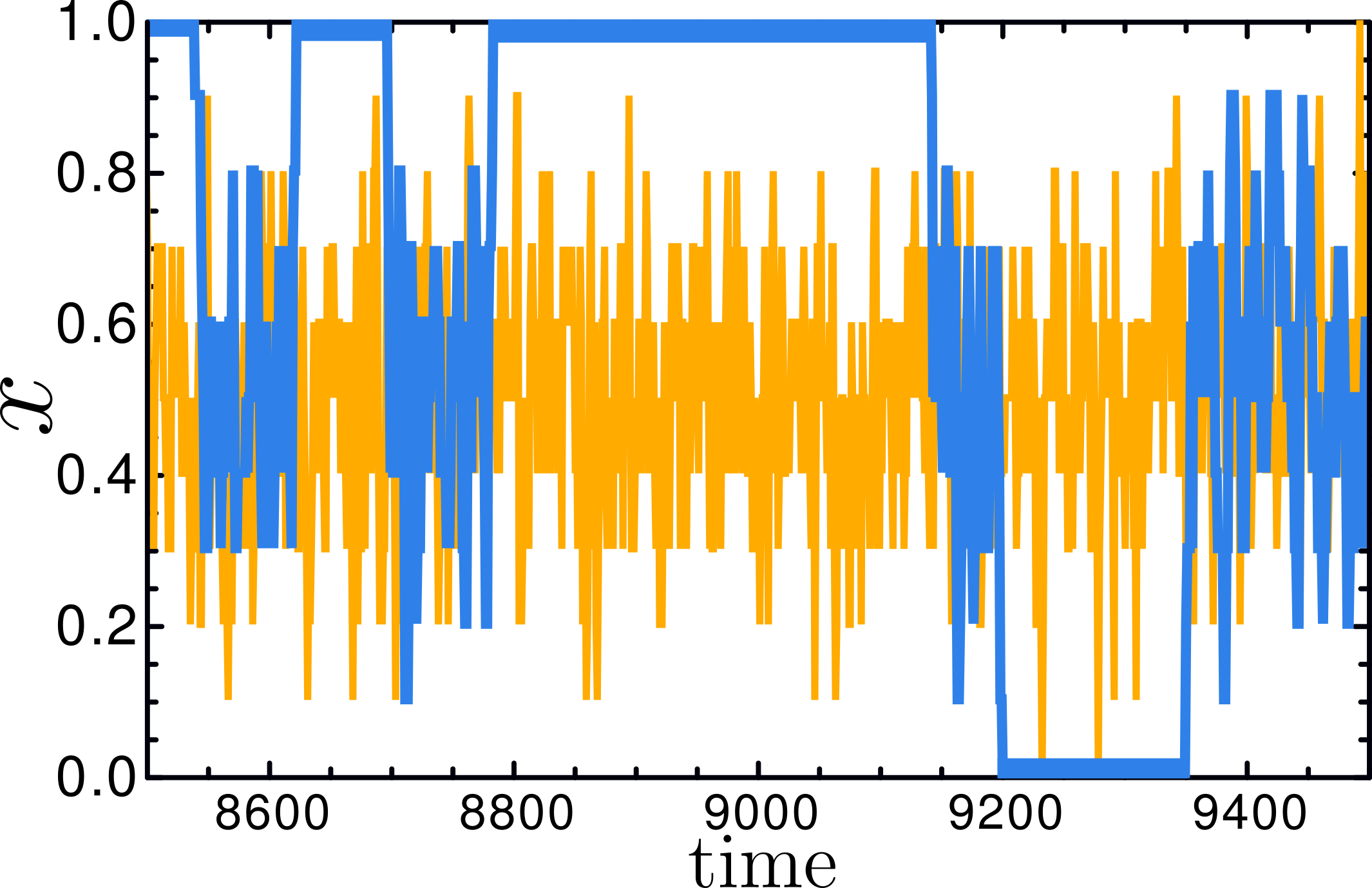
Figure 6: Typical population trajectories in composition space for $\lambda/\lambda_{c}=2\times 10^{-3}$ (blue) and $\lambda/\lambda_{c}=2$ (orange) for the case $N=10$.

One way to quantify these fluctuations is by the return time $RT$, which we define as the time interval between successive points where $x=\frac{1}{2}$. As suggested by Fig. 6, this return time will be short for $\lambda\gg\lambda_{c}$ and become long for $\lambda\ll\lambda_{c}$. The latter behavior is a harbinger of large composition fluctuations in the population. We can again use the backward Kolmogorov approach to determine the $\lambda$ dependence of the return time. Let $\tau_{n}$ denote the average time to reach the balanced state of equal numbers of A’s and B’s when starting from a state where the number of A’s equals $n>\frac{1}{2}N$. Then

$$RT=\frac{1}{N}+\tau_{1+N/2}\,.$$ (24)

That is, starting from the balanced state, the average return time to this state is the average time for a single event, $\frac{1}{N}$, where the population now consists of $\frac{N}{2}+1$ A’s and $\frac{N}{2}-1$ B’s, plus the average time to reach the balanced state when starting from this minimally imbalanced state.

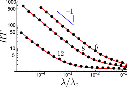
Figure 7: Dependence of the return time $RT$ on $\lambda/\lambda_{c}$ for various values of $N$.

In analogy with Eq. (9) for the fixation time, the time $\tau_{n}$ satisfies the recursion

$$\tau_{n} =(1-\lambda)\left[a_{n}\tau_{n+1}+b_{n}\tau_{n-1}+\big{(}1-a_{n}-b_{n}\big{)}\tau_{n}\right]$$

$$\qquad\qquad+\lambda\left[c_{n}\tau_{n+1}+d_{n}\tau_{n-1}+\big{(}1-c_{n}-d_{n}\big{)}\tau_{n}\right]+\delta t\,,$$ (25a)

with $$a_{n} b_{n} c_{n} d_{n}$$, given by (1a) and (1b), and , given by (19). We can rewrite this recursion in the canonical form of Eq. (9):

$$\tau_{n}=a_{n}^{\prime}\tau_{n+1}+b_{n}^{\prime}\tau_{n-1}+(1-a_{n}^{\prime}-b_{n}^{\prime})\tau_{n}+\delta t\,,$$ (25b)

where $a_{n}^{\prime}=(1-\lambda)a_{n}+\lambda c_{n}$ and $b_{n}^{\prime}=(1-\lambda)b_{n}+\lambda d_{n}$. This recursion is valid for $\frac{1}{2}N<n<N$, while for $n=N$ the first term in (25b) is absent. This missing term acts as the effective reflecting boundary condition for $n=N$. At $n=\frac{1}{2}N$, the appropriate boundary condition is $\tau_{N/2}=0$; namely, the balanced state corresponds to the end of the process. The result for $\tau_{n}$ for arbitrary $n$ is given in (43), while the return time $RT$ itself is given in (42) (see D for details). Figure 7 shows that $RT$ scales as $\lambda^{-1}$ for $\lambda\to 0$. This behavior is the source of the long-lived temporal fluctuations in the composition of the population, as illustrated in Fig. 6.

6 Discussion

Much of the literature on populations of multiple cooperating species has focused on the continuous limit. Such a population is driven to an attractor state in which there are equal concentrations of each species. However, when finite-population stochasticity is incorporated, the true attractors of the dynamics of an isolated population are instead the fixation states, in which only one species exists. Because stochastic effects are relevant in real systems, a discrete approach that incorporates this stochasticity is necessary to describe the dynamics in a faithful way.

Within the discrete approach, we determined the probability for a finite population to reach a given fixation state as a function of the initial condition, as well as the time to reach fixation. The behaviors of these two quantities reflect the effective bias that drives the system to the quasi-steady state of equal concentrations of the two species. Namely, the fixation probability is nearly independent of the initial condition and the fixation time scales exponentially with population size $N$. As a consequence of this exponential dependence, fixation is not observable in a laboratory or in a simulational time scale for any reasonable population size.

It is worth mentioning that the statistical features of two-species cooperation share similarities with the vacillating voter model [40], despite their different microscopic update rules. In the vacillating voter model, agents (voters) can be in one of two voting states and their agreement or disagreement is influenced by the state of yet another neighbor. Here “vacillation” refers to the possibility that a voter does not adopt the state of a randomly chosen neighbor, as in the standard voter model, but may adopt the state of this additional neighbor. The properties of this decision process drives the population toward a zero-magnetization state. This state is equivalent to the attractor in two-species cooperation, where both species are equally represented.

When migration into the system can also occur, the population now ostensibly reaches a steady state. An unanticipated feature of this steady state for small migration rate $\lambda$ is that this state is not genuinely steady, because there are long-term stochastic fluctuations that drive the population from one near-fixation state to the opposite near-fixation state, with the population spending long time periods in these near-fixation states. Such macroscopic wanderings are reflected in the steady-state abundance distribution, which is strongly peaked at these near-fixation states for sufficiently small $\lambda$. The time scale associated with these fluctuations increases rapidly as the migration rate decreases. Thus observations of a cooperative system have to be sufficiently long to incorporate many such wanderings so as to ensure that true average behavior is actually probed. We found that the return time—the time between successive instants where the number of A’s and B’s are equal—allows us to quantify these temporal fluctuations in a precise way.

This observation of large fluctuations also has important ramifications for populations that consist of more than two cooperating species. Depending the immigration rate, the population size $N$, and the number of distinct species $S$, the number of species that are actually present at any given time could be much less than $S$. Thus a typical steady state could have a very different character than the average steady state that is predicted by the time-independent density distribution. Moreover, a multispecies population will also exhibit large fluctuations in the actual composition of the species that are present. This intriguing issue has recently been investigated in the context of multispecies Lotka-Volterra models [41, 42]. The backward Kolmogorov equation offers the possibility of obtaining new insights into these large fluctuations because of the relative simplicity of neutral models of cooperating species.

The predictions presented in our study can also be tested in experimental settings that are based on microfluidic chambers, where small populations of cells can be maintained so that long-term monitoring can be performed. These small-scale devices offer a unique opportunity to explore the impact of population size and validate the approximations presented in this work. Both well-mixed populations, as well as two- and there-dimensional spatial populations, could be maintained in constant numbers over time. Future extensions of our model, such as including cell death or environmental noise, would be helpful to design experimental protocols and explore the conditions required to maintain stable cooperative cell assemblies [43, 44].

Acknowledgments

The authors thank Deepak Bhat and Jacopo Grilli for fruitful discussions, and Eric A. Blair for inspiring ideas. JP and RS were supported by the Botín Foundation and the Spanish Ministry of Economy and Competitiveness through grant FIS2015-67616-P MINEICO/AEI/FEDER. JP is also supported by ”María de Maeztú” fellowship MDM-2014-0370-17-2. SRs research was supported in part by NSF grant DMR-1910736. JP and RS thank the hospitality of the Santa Fe Institute, where this project began.

Appendix A The Fixation Probability

We want to solve Eq. (7) for the fixation probability:

$$E_{n}=a_{n}E_{n+1}+b_{n}E_{n-1}+\big{(}1-a_{n}-b_{n}\big{)}E_{n}\,.$$

This calculation is standard (see, e.g., [45]) and we provide it here so that our presentation is self contained. It is convenient to rewrite the above equation as $a_{n}(E_{n+1}-E_{n})=b_{n}(E_{n}-E_{n-1})$, and then define $u_{n}\equiv E_{n}-E_{n-1}$ and $r_{n}\equiv b_{n}/a_{n}$ to recast it as the following first-order recursion for the $u_{n}$:

$$u_{n}=r_{n-1}\,u_{n-1}=r_{n-1}\,r_{n-2}\,r_{n-2}\cdots r_{1}\,u_{1}\,,$$

with $u_{1}=E_{1}-E_{0}=E_{1}$. We now define $R_{n}=\prod_{m=1}^{n}r_{m}$ so that the equation for $u_{n}$ becomes

$$u_{n}=R_{n-1}\,u_{1}=R_{n-1}\,E_{1}\,.$$ (26)

Since the $u_{n}$ are successive differences of the $E_{n}$, we determine $E_{n}$ by summing the $u_{n}$. Thus

$$E_{n}=\sum_{m=1}^{n}u_{m}=\sum_{m=1}^{n}R_{m-1}\,E_{1}=\sum_{m=0}^{n-1}R_{m}\,E_{1}\,,$$ (27)

where we need to define $R_{0}=1$ for consistency. We now determine the unknown $E_{1}$ by using the boundary condition $E_{N}=1$ in (27) to give $E_{N}=\sum_{m=0}^{N-1}R_{m}\,E_{1}=1$. Having found $E_{1}$, the general solution for $E_{n}$ is

$$E_{n}=\sum_{m=0}^{n-1}R_{m}\,\Big{/}\sum_{m=0}^{N-1}R_{m}\,,$$ (28)

To simplify the above expression, we start with $a_{n}$ and $b_{n}$ defined in Eq. (1):

$$a_{n}=\frac{n}{N}\left(1-\frac{n}{N}\right)^{2}\qquad b_{n}=\left(\frac{n}{N}\right)^{2}\left(1-\frac{n}{N}\right)\,,$$

so that $r_{n}=b_{n}/a_{n}=n/(N-n)$. Then

$$R_{n} =r_{1}\,r_{2}\,\ldots r_{n}=\frac{n!(N-n-1)!}{(N-1)!}=\left[\binom{N-1}{n}\right]^{-1}\,.$$

Substituting this representation for $R_{n}$ in (28) gives Eq. (8).

For completeness, we also give the continuum solution for the fixation probability. We take the continuum limit of Eq. (7) by letting $(n\pm 1)/N\to x\pm dx$, with $dx=\frac{1}{N}$, and then expanding this equation to second order in $dx$. This gives

$$E^{\prime\prime}+2N(1-2x)E^{\prime}=0\,,$$ (29)

where the prime denotes differentiation with respect to $x$. This equation is subject to the boundary conditions $E(0)=0$ and $E(1)=1$. As in the discrete formulation, the first condition corresponds to the impossibility of reaching a population of all A’s if the initial state contains no A’s, while the second condition corresponds to the initial state coinciding with the desired final state. The solution to (29), subject to the given boundary conditions is

$$E(x)=\frac{{\displaystyle\int_{0}^{x}du\,e^{2N(u^{2}-u)}}}{{\displaystyle\int_{0}^{1}du\,e^{2N(u^{2}-u)}}}=\frac{1}{2}\left[1+\frac{\text{erfi}\big{(}\sqrt{2N}(x-\frac{1}{2})\big{)}}{\text{erfi}(\sqrt{N/2})}\right]\,,$$ (30)

where erfi is the imaginary error function. This expression from the continuum approximation agrees well with the exact discrete result (8) (see Fig. 3). However, the continuum approach is no longer accurate for the fixation time (see the next section).

Appendix B The Fixation Time

We now solve the recursions (9) for the fixation time:

$$T_{n} =a_{n}T_{n+1}+b_{n}T_{n-1}+\big{(}1-a_{n}-b_{n}\big{)}T_{n}+\delta t\,.$$

Following the same steps that led to (26), we obtain, for the difference $v_{n}\equiv T_{n}-T_{n-1}$,

$$v_{n}=r_{n-1}\,v_{n-1}-\alpha_{n-1}\,,$$ (31)

where $\alpha_{n}\equiv\delta t/a_{n}$. Notice that $v_{1}=T_{1}-T_{0}=T_{1}\equiv R_{0}\,T_{1}$.

We develop the recursion (31) to give

$$v_{n} =r_{n-1}\,r_{n-2}\,v_{n-2}-\alpha_{n-1}-r_{n-1}\,\alpha_{n-2}$$

$$=r_{n-1}\,r_{n-2}\,r_{n-3}\,v_{n-3}-\alpha_{n-1}-r_{n-1}\,\alpha_{n-2}-r_{n-1}\,r_{n-2}\,\alpha_{n-3}$$

$$\hskip 85.35826pt\vdots$$

continuing this development to the end leads to

$$v_{n}=R_{n-1}\,v_{1}-Q_{n-1}=R_{n-1}\,T_{1}-Q_{n-1}\,,$$ (32)

where

$$Q_{n}\equiv\alpha_{n}+r_{n}\,\alpha_{n-1}+r_{n}\,r_{n-1}\,\alpha_{n-2}+\cdots+r_{n}\,r_{n-1}\cdots r_{2}\,\alpha_{1}\,,$$

and $Q_{0}=0$ by virtue of (32).

Finally, we sum the $v_{n}$ to obtain the fixation time:

$$T_{n}=\sum_{m=1}^{n}v_{m}=\sum_{m=0}^{n-1}R_{m}\;T_{1}-\sum_{m=1}^{n-1}Q_{m}$$ (33)

To eliminate the unknown $T_{1}$, we use the boundary condition $T_{N}=0$ to give

$$T_{1}=\sum_{m=1}^{N-1}Q_{m}\Big{/}\sum_{m=0}^{N-1}R_{m}\,.$$

Substituting this in (33) and noting that $\sum_{m=0}^{n-1}R_{m}/\sum_{m=0}^{N-1}R_{m}$ is just the fixation probability $E_{n}$, we obtain the result quoted in Eq. (10).

Appendix C WKB Approximation

A comprehensive review of the application of the WKB method for large deviations in stochastic populations can be found in [26]. In this section we summarize the basic steps to reach Eq. (13). We make the ansatz $\tilde{P}(x)\sim\exp\left\{NS_{0}(x)+S_{1}(x)+O\left(N^{-1}\right)\right\}$, and expand to linear order in $\delta x$ to give

$$\tilde{P}(x\pm\delta x)\simeq\tilde{P}(x)\exp\left\{\pm S_{0}^{\prime}+\delta x\left(\frac{S_{0}^{\prime\prime}}{2}\pm S_{1}^{\prime}\right)\right\}\simeq\ \tilde{P}(x)e^{\pm S_{0}^{\prime}}\left[1+\delta x\left(\frac{S_{0}^{\prime\prime}}{2}\pm S_{1}^{\prime}\right)\right]\,,$$

with $\delta x=1/N$. We now define $\Lambda\equiv e^{S_{0}^{\prime}}$ and substitute this into (12) to obtain

$$\left(a-a^{\prime}\delta x\right)\Lambda^{-1}\left[1+\delta x\left(\frac{S_{0}^{\prime\prime}}{2}-S_{1}^{\prime}\right)\right]+\left(b+b^{\prime}\delta x\right)\Lambda\left[1+\delta x\left(\frac{S_{0}^{\prime\prime}}{2}+S_{1}^{\prime}\right)\right]=a+b\,,$$

which can be separated into terms of $O(1)$ and terms of $O(\delta x)$. For the former, we have

$$a\Lambda^{-1}+b\Lambda=a+b\,,$$ (34)

which has the two solutions $\Lambda_{0}=1$ and $\Lambda=\frac{a}{b}$. The $\Lambda_{0}$ solution corresponds to $S_{0}^{\prime}=0$, and the resulting constant can be absorbed by the normalization condition on $\tilde{P}(x)$. The second solution is

$$S_{0}^{\prime}=\log\left(\frac{a}{b}\right)\,,$$ (35)

which, after integration, results in the first expression in (13). For the $O(\delta x)$ terms we must solve

$$-a^{\prime}\Lambda^{-1}+a\Lambda^{-1}\left(\frac{S_{0}^{\prime\prime}}{2}-S_{1}^{\prime}\right)+b^{\prime}\Lambda+b\Lambda\left(\frac{S_{0}^{\prime\prime}}{2}+S_{1}^{\prime}\right)=0\,,$$ (36)

which, after substitution of $\Lambda=\frac{a}{b}$, yields

$$b\left(\frac{S_{0}^{\prime\prime}}{2}-S_{1}^{\prime}\right)+a\left(\frac{S_{0}^{\prime\prime}}{2}+S_{1}^{\prime}\right)=b\frac{a^{\prime}}{a}-a\frac{b^{\prime}}{b}\;.$$ (37)

On the other hand, $S_{0}^{\prime\prime}=\frac{a^{\prime}}{a}-\frac{b^{\prime}}{b}$, which reduces the previous equation to

$$(a-b)S_{1}^{\prime}=\frac{1}{2}\left[b\;\frac{a^{\prime}}{a}-a\;\frac{b^{\prime}}{b}-(a^{\prime}-b^{\prime})\right]=-\frac{1}{2}\left(\frac{a^{\prime}}{a}+\frac{b^{\prime}}{b}\right)(a-b)\ .$$ (38)

The first term in the brackets on the right-hand side corresponds to the derivative of $\log(ab)$. Hence, after integration, we obtain the second expression in (13).

Appendix D The Return Time

We want to solve the recursion for the return time $\tau_{n}$, defined as the time for the population to first reach the state with equal numbers of A’s and B’s when the initial state contains $n>\frac{1}{2}N$ A’s. The state with $n=N$ plays the role of an effective reflecting boundary condition. The system of equations that we wish to solve is (25b):

$$\tau_{n}=a_{n}^{\prime}\tau_{n+1}+b_{n}^{\prime}\tau_{n-1}+(1-a_{n}^{\prime}-b_{n}^{\prime})\tau_{n}+\delta t\,,$$ (39a)

for $$1+N/2\leq n<N n=N$$, while for the appropriate equation is

$$\tau_{N}=b_{B}^{\prime}\tau_{N-1}+(1-a_{N}^{\prime}-b_{N}^{\prime})\tau_{N}+\delta t\,.$$ (39b)

Using the fact that $a_{N}^{\prime}=0$, this last equation can be rewritten as

$$\tau_{N}-\tau_{N-1}\equiv v_{N}=\frac{\delta t}{b_{N}^{\prime}}\,.$$ (40)

The remaining $\frac{N}{2}-1$ equations (39a) are of the same type as (9) for the fixation time. Thus the solution for $\tau_{n}$ has the same form as (33):

$$\tau_{n}=\sum_{m=N/2}^{n-1}R_{m}^{\prime}\;\tau_{1+N/2}\;-\!\!\sum_{m=1+N/2}^{n-1}Q_{m}^{\prime}\,,$$ (41)

where

$$R_{n}^{\prime}=\prod_{m=1+N/2}^{n}\frac{b_{n}^{\prime}}{a_{n}^{\prime}}\equiv\prod_{m=1+N/2}^{n}r_{n}^{\prime}$$

and

$$Q_{n}^{\prime}=\alpha_{n}^{\prime}+r_{n}^{\prime}\,\alpha_{n-1}^{\prime}+r_{n}^{\prime}\,r_{n-1}^{\prime}\,\alpha_{n-2}^{\prime}+\cdots+r_{n}^{\prime}\,r_{n-1}^{\prime}\cdots r_{2+N/2}^{\prime}\,\alpha_{1+N/2}^{\prime}\,,$$

with $\alpha_{n}^{\prime}=\delta t/a_{n}^{\prime}$ and and $Q_{N/2}^{\prime}=0$.

To eliminate the unknown $\tau_{1+N/2}$, we now write (41) for the special cases of $n=N$ and $n=N-1$:

$$\tau_{N}=\sum_{m=N/2}^{N-1}R_{m}^{\prime}\;\tau_{1+N/2}\;-\!\!\sum_{m=1+N/2}^{N-1}Q_{m}^{\prime}\qquad\qquad\tau_{N-1}=\sum_{m=N/2}^{N-2}R_{m}^{\prime}\;\tau_{1+N/2}\;-\!\!\sum_{m=1+N/2}^{N-2}Q_{m}^{\prime}\,.$$

Their difference is

$$\tau_{N}-\tau_{N-1}=R_{N-1}^{\prime}\,\tau_{1+N/2}-Q_{N-1}^{\prime}=\frac{\delta t}{b_{N}^{\prime}}\,,$$

so that $\tau_{1+N/2}$ is given by

$$\tau_{1+N/2}=\frac{Q_{N-1}^{\prime}+\delta t/b_{N}^{\prime}}{R_{N-1}^{\prime}}\,.$$ (42)

Substituting this expression for $\tau_{1+N/2}$ in (41) gives the average time to reach the balanced state of equal numbers of A’s and B’s when starting from a population that contains $n$ A’s with a reflecting boundary condition at $n=N$:

$$\tau_{n}=\sum_{m=N/2}^{n-1}R_{m}^{\prime}\;\frac{Q_{N-1}^{\prime}+\delta t/b_{N}^{\prime}}{R_{N-1}^{\prime}}-\sum_{m=1+N/2}^{n-1}Q_{m}^{\prime}\,.$$ (43)

What we want, however, is, the return time, defined as the average time to start at the balanced state and first return to this state. This is $RT=\frac{1}{N}+\tau_{1+N/2}$.

References

- [1] Goel N S, Maitra S C and Montroll E W 1971 Reviews of Modern Physics 43 231
- [2] Murray J D 2007 Mathematical Biology: I. An Introduction vol 17 (Springer Science & Business Media)
- [3] May R M 2019 Stability and Complexity in Model Ecosystems vol 1 (Princeton University Press)
- [4] May R M, Levin S A and Sugihara G 2008 Nature 451 893–894
- [5] Bronstein J L 2015 Mutualism (Oxford University Press, USA)
- [6] Perc M 2016 Physics Letters A 380 2803–2808
- [7] Perc M, Jordan J J, Rand D G, Wang Z, Boccaletti S and Szolnoki A 2017 Physics Reports 687 1–51
- [8] Mitri S, Clarke E and Foster K R 2016 The ISME Journal 10 1471–1482
- [9] Nadell C D, Drescher K and Foster K R 2016 Nature Reviews Microbiology 14 589–600
- [10] Müller M J, Neugeboren B I, Nelson D R and Murray A W 2014 Proceedings of the National Academy of Sciences 111 1037–1042
- [11] Shou W, Ram S and Vilar J M 2007 Proceedings of the National Academy of Sciences 104 1877–1882
- [12] Amor D R, Montañez R, Duran-Nebreda S and Solé R 2017 PLoS Computational Biology 13 e1005689
- [13] Rodríguez Amor D and Dal Bello M 2019 Life 9 22
- [14] Nowak M A 2006 Evolutionary Dynamics: Exploring the Equations of Life (Harvard University Press)
- [15] Antal T and Scheuring I 2006 Bulletin of Mathematical Biology 68 1923–1944
- [16] Altrock P M and Traulsen A 2009 New Journal of Physics 11 013012
- [17] Black A J, Traulsen A and Galla T 2012 Physical Review Letters 109 028101
- [18] Nadell C D, Foster K R and Xavier J B 2010 PLoS Computational Biology 6 e1000716
- [19] Rakoff-Nahoum S, Foster K R and Comstock L E 2016 Nature 533 255–259
- [20] Foster K R, Schluter J, Coyte K Z and Rakoff-Nahoum S 2017 Nature 548 43–51
- [21] Friedman J and Gore J 2017 Current opinion in Systems Biology 1 114–121
- [22] Vega N M and Gore J 2018 Current opinion in microbiology 45 195–202
- [23] Elgart V and Kamenev A 2004 Physical Review E 70 041106
- [24] Kessler D A and Shnerb N M 2007 Journal of Statistical Physics 127 861–886
- [25] Assaf M and Meerson B 2010 Physical Review E 81 021116
- [26] Assaf M and Meerson B 2017 Journal of Physics A: Mathematical and Theoretical 50 263001
- [27] Krapivsky P L, Redner S and Ben-Naim E 2010 A Kinetic View of Statistical Physics (Cambridge University Press)
- [28] Van Kampen N G 1992 Stochastic Processes in Physics and Chemistry vol 1 (Elsevier)
- [29] Redner S 2001 A Guide to First-Passage Processes (Cambridge University Press)
- [30] URL https://math.stackexchange.com/questions/151441/calculate-sums-of-inverses-of-binomial-coefficients
- [31] Moran P A P et al. 1962 The Statistical Processes of Evolutionary Theory
- [32] Kimura M 2020 The neutral theory and molecular evolution My Thoughts on Biological Evolution (Springer) pp 119–138
- [33] Ewens W J 2012 Mathematical Population Genetics 1: Theoretical Introduction vol 27 (Springer Science & Business Media)
- [34] Bender C M and Orszag S A 2013 Advanced mathematical methods for scientists and engineers I: Asymptotic methods and perturbation theory (Springer Science & Business Media)
- [35] Gardiner C W et al. 1985 Handbook of Stochastic Methods vol 3 (Springer Berlin)
- [36] Fichthorn K, Gulari E and Ziff R 1989 Physical Review Letters 63 1527
- [37] Considine D, Redner S and Takayasu H 1989 Physical Review Letters 63 2857
- [38] Carro A, Toral R and San Miguel M 2016 Scientific reports 6 1–14
- [39] Herrerías-Azcué F and Galla T 2019 Physical Review E 100 022304
- [40] Lambiotte R and Redner S 2007 Journal of Statistical Mechanics: Theory and Experiment 2007 L10001
- [41] Bunin G 2017 Physical Review E 95 042414
- [42] Pearce M T, Agarwala A and Fisher D S 2020 Proceedings of the National Academy of Sciences 117 14572–14583
- [43] Ferry M S, Razinkov I A and Hasty J 2011 Microfluidics for synthetic biology: from design to execution Methods in Enzymology vol 497 (Elsevier) pp 295–372
- [44] Luke C S, Selimkhanov J, Baumgart L, Cohen S E, Golden S S, Cookson N A and Hasty J 2016 ACS Synthetic Biology 5 8–14
- [45] Karlin S and Taylor H M 2014 A First Course in Stochastic Processes (Academic Press)