Accelerating GMRES with Deep Learning in Real-Time

Abstract

GMRES is a powerful numerical solver used to find solutions to extremely large systems of linear equations. These systems of equations appear in many applications in science and engineering. Here we demonstrate a real-time machine learning algorithm that can be used to accelerate the time-to-solution for GMRES. Our framework is novel in that is integrates the deep learning algorithm in an in situ fashion: the AI-accelerator gradually learns how to optimizes the time to solution without requiring user input (such as a pre-trained data set).

We describe how our algorithm collects data and optimizes GMRES. We demonstrate our algorithm by implementing an accelerated (MLGMRES) solver in Python. We then use MLGMRES to accelerate a solver for the Poisson equation – a class of linear problems that appears in may applications. Informed by the properties of formal solutions to the Poisson equation, we test the performance of different neural networks. Our key takeaway is that networks which are capable of learning non-local relationships perform well, without needing to be scaled with the input problem size, making them good candidates for the extremely large problems encountered in high-performance computing. For the inputs studied, our method provides a roughly 2$\times$ acceleration.

1 Introduction

The list of scientific problems that are modeled by partial differential equations (PDEs) is vast. A numerical solution to a PDE is therefore incredibly useful for the study of the complex relationships arising in the world around us. From the study of microscopic particle interactions [1] to the study of massive astronomical objects and nearly every length scale in between, solutions to PDEs are needed [2, 3]. In practice, most applications require solutions to these PDEs as a function of time. This often requires the numerical computation of these PDEs at many instances called “time steps”. At these time steps, solvers are employed to compute solutions. The precise details of these solvers depends highly on the mathematical properties and scientific context of the underlying problem being solved. Despite this large variation in methods used to obtain solutions to PDEs, there is often overlap in some of the details of these methods. For example more often than not, at some point a linear problem will need to be solved using iterative methods – i.e. the solution is refined with each iteration. The rate at which these methods converge to the final solution varies substantially with the problem and tends to depend on initial information provided to the solver. This initial information often takes the form of a problem-specific initial guess or a problem-specific transformation (a preconditioner) that leads to more agreeable convergence properties. Consequently, the performance of these methods can be significantly improved by supplying such initial conditions and preconditioners [4]. In practice, finding effective initial guesses and preconditioners (if any can be found at all using existing methods) for a particular problem is very much an art that requires thoughtful input from an expert. In addition to accelerating simulations through algorithmic optimizations (such as finding better choices for preconditioners), we see great potential in taking advantage of the rapid improvements in hardware targeting machine learning applications.

As high-performance computing paradigms shift towards ever increasing heterogeneity, the abundance of accelerators aimed at machine learning applications provide an increasingly attractive opportunity to make use of these resources to accelerate traditional scientific simulations [5, 6, 7, 8, 9, 10, 11, 12]. Enabled by the presence of these accelerators in HPC systems, we envision using neural networks to learn efficient preconditioners and initial guesses for simulations with underlying iterative linear solvers in real-time. To demonstrate the merits of this idea, here we develop a real-time deep learning powered accelerator for GMRES [13] applied to second-order linear partial differential equations. Countless applications in heat flow, diffusion phenomena, wave propagation, fluid flow, electrodynamics, quantum mechanics, and much more are faithfully modeled by linear second order PDEs. Consequently, by building a foundation on such a useful class of problems, we are able to establish out of the gate that the underlying ideas introduced here inherently posses the potential to be useful for a wide range of problems of practical importance.

Broadly speaking, we aim to utilize deep learning to accelerate PDE-based simulations by training and applying these learned preconditioners in real-time. We emphasize that the goal here is to accelerate a simulation in real-time when we do not have access to relevant data prior to the start of the simulation. In particular, we demonstrate that we can train a neural network in real-time to learn preconditioners as a simulation runs – improving the speed of the underlying linear solver and decreasing the overall wall-clock-time of the simulation. In shifting our focus to accelerating the solver in real-time while data is being generated, some non-standard challenges are encountered. Among these challenges, we must deal with the fact that we are working with new data in a quasi-online fashion as it becomes available over the course of our simulation. In other words, we do not necessarily (and often do not) have access to a representative distribution of data as our simulation progresses. Another key challenge when working in real-time lies in the selection and training of a model. Simply put, if our learned model is to be constructed and used in real time to accelerate a simulation, the training time scale cannot be comparable to the time scale of the simulation. Owing to these challenges, working with neural networks in real-time with limited incoming data ("online") is difficult. We overcome these challenges with deep learning for the problem at hand by carefully selecting a model that aims to accelerate the underlying solver rather than accurately learn the solution i.e. we are not merely learning a look-up table for the solution given the inputs), and by curating the training set as it grows in real-time so that the neural network is able to improve performance before a representative distribution of data is attained.

1.1 The Case for Online Acceleration vs. Offline End-to-End Learning

While deep learning has shown great potential in producing models that capture complex relationships in scientific applications and even discovering such relationships, some key underlying difficulties have persisted despite this progress [14, 15].

In the space of scientific simulation and modeling, there are two such difficulties. The first is the “trust problem”: how do we trust the result of a neural network? A common approach is to treat outputs from neural networks as probabilistic, thus treating outputs as confidence intervals. This might work well, e.g. if the goal is to predict the preferences of most customers. However there is little room for uncertainty when solving PDEs: a mathematical object either satisfies the PDE – i.e. it is a solution – or it does not. The second difficulty is that most machine learning workflows assume that data is both cheaply and readily available. While this is not a bad assumption for many commercial applications, in the field of high-performance computing data is usually generated on specialized, expensive, and highly sought-after hardware. We therefore need to consider data produced on HPC systems as valuable and difficult to come by. Moreover, scientific data generalizes poorly, e.g. different applications will use slightly different PDEs, as well as modeling and temporal resolutions. Hence, it is hard to estimate in advance how big a training set needs to be in order to accelerate a particular problem.

First we address the issue of trust by treating the trained model as an in situ component of the solver. Iterative solvers give us the unique opportunity to to do this in a strait forward way: we can always use the “final iteration” of our solver to ensure that the PDE is satisfied. With regards to the expense of the collected data, the approach we propose also deals with this challenge. We have implemented a real-time “online” learning algorithm where all relevant data is localized to the problem being solved. Our code keeps a history of the time steps being simulated and gradually grows the training set. Consequently, there is no need to pre-compute massive data sets that sufficiently span a wide range of the solution space so that the learned model would (hopefully) generalize well.

In a nutshell, by using deep learning as a flexible in situ accelerator for iterative methods in real-time rather than as a means to fit a surrogate model, we are able to harness the intrinsic strength of deep learning and dedicated hardware/software to produce useful science without the typical challenges common to machine learning in computational science.

1.2 A Class of Problems and Their Computational Cost

In a PDE-based simulation, one usually starts with a time-dependent partial differential equation (or a system of such equations) on some domain $\Omega$, with some initial and boundary conditions. A simple example of such a problem is

$$\frac{\partial u\left(\mathbf{x},t\right)}{\partial t}=R(u\left(\mathbf{x},t\right)),$$ (1)

$$u(\mathbf{x},0)=g(\mathbf{x}),\ \mathbf{x}\in\Omega,$$ (2)

$$u(\mathbf{x},t)=h(\mathbf{x},t)+\frac{\partial u(\mathbf{x},t)}{\partial n},\ \mathbf{x}\in\partial\Omega,$$ (3)

where $R(u)$ is some operator (which can be linear or nonlinear), $g$ is some initial condition, and $h$ is the prescribed value on the boundary of the solution along with the normal derivative of the solution along the boundary of the domain. To numerically solve this problem, one discretizes in space and time. The choice of these discretizations depend on factors such as desired accuracy of the solution, scales of interest in the problem, and mathematical properties of the underlying solutions among many factors. Regardless of the method chosen, the problem at hand, and the desired accuracy, at some point a solution to a linear system of equations which takes the form:

$$\mathbf{A}x=\mathbf{b},$$ (4)

is required. In practice, as both the desired resolution $n$ and dimension $d$ of the problem grows, the size of this linear system is $O(n^{2d})$ and becomes so large that it is infeasible to explicitly store the matrix $A$, let alone use exact direct solution methods that require $O(n^{6d})$ operations to attain a solution [16]. As this is infeasible for any realistic $n$, iterative methods for linear problems are standard because they require at most $O(n^{4d})$ number of operations to reach machine precision and can be stopped far earlier to a desired accuracy. A successful class of these iterative methods are known as Krylov Subspace methods [16]. In general, these methods work by projecting the original $O(n^{2d})$ dimensional problem into a lower dimensional Krylov subspace $K_{m}(\mathbf{A},\mathbf{b})\subset\mathbb{R}^{n^{d}}$ spanned by the Krlov sequence $\{\mathbf{b},\mathbf{A}\mathbf{b},\mathbf{A}^{2}\mathbf{b},\dots,\mathbf{A}^{m-1}\mathbf{b}\}$. The convenience and efficiency of these methods is particularly clear when one takes notice of the fact that the Krylov sequence can be formed by repeatedly applying the matrix operator rather than explicitly needing to construct and store the matrix $\mathbf{A}$ itself $\{\mathbf{b},\mathbf{A}(\mathbf{b}),\mathbf{A}(\mathbf{A}(\mathbf{b})),\mathbf{A}(\mathbf{A}(\mathbf{A}(\mathbf{b}))),\dots\}$. While many successful methods for linear systems fall under Krylov subspace methods such as Generalized Minimal Residuals (GMRES), Conjugate Gradient (CG), Biconjugate Gradients (BCG) and its many variants [16], we focus on GMRES to illustrate our data-driven approach to accelerate a simulation. In particular, we focus on a particular form of GMRES known as $k$-step restarted GMRES or GMRES($k$) that restarts GMRES iterations using the final previous GMRES iteration as new initial guess. Restarting the algorithm is essential when the number of operations and storage requirements are prohibitively large. In this work, we focus on accelerating GMRES($k$) as it is a common choice to solve the Poisson equation – or in the case of 3-dimensional problems, the Laplace equation [1].

While GMRES is a powerful method, like any iterative method, a good initial guess can vastly improve performance of the method. That said, it is well known that initial guesses that do not incorporate problem related information can negatively impact the performance of GMRES [17]. However, with deep learning we aim to show that we can learn effective initial guesses that accelerate GMRES in real-time, effectively acting as left preconditioners since no extra work is needed once a solution is obtained. The reason that these learned initial guesses we supply to GMRES can effectively act like left preconditioners lies in the fact that our model learns initial guesses that aim to optimize both the initial residual and the rate of convergence of GMRES simultaneously.

1.3 Accelerating GMRES

Historically, accelerating GMRES through good initial guesses has been difficult to achieve and typically poses a high risk since performance can degrade with guesses that do not somehow incorporate problem specific information [17]. Furthermore, it is standard knowledge among practitioners that simply reducing the normalized initial error through a naively constructed initial guess (such as a solution interpolated from a coarse grid) will not improve convergence behavior of GMRES. However, we find that deep learning can be used to train a model that will take in a problem and propose an optimal initial guess. To point out how the rate of GMRES can be accelerated with only an initial guess, consider the Krylov space that GMRES constructs when a non-zero initial guess $x^{0}$ is used. In this case, the initial residual is given by $r^{0}=\mathbf{A}x^{0}-b$ rather than just $b$ as demonstrated earlier. Then, the $n$-th Krylov subspace is given by $K_{n}(\mathbf{A},r^{0})=\text{span}\{r^{0},\mathbf{A}r^{0},\mathbf{A}^{2}r^{0},\dots,\mathbf{A}^{n-1}r^{0}\}$. Since the structure of the initial residual has the potential to influence every Krylov space element, a good initial guess that encodes problem related information has the potential to not just reduce the initial residual $r^{0}=\mathbf{A}x^{0}-b$, but also simultaneously accelerate the rate at which GMRES converges.

We emphasize here that initial guesses have the potential to improve both the initial residual $r^{0}$ and the rate of convergence of GMRES. Improving the initial residual $r^{0}$ using a neural network is straightforward, however improving the rate of convergence of GMRES using deep learning is more subtle. The primary reason for this is that a guess that improves the initial residual $r^{0}$ does not necessarily imply that GMRES will solve the problem at an accelerated rate. In the approach we outline here, we construct a neural network that encodes the problem, and use the fact that we are working in real-time to be able to asses whether initial guesses provided by the neural network are improving the rate of convergence. To be more precise, we monitor the performance in order to be able to use real-time performance metrics to decide what data should be added to the training set and when the neural network should be trained in order to accelerate performance.

1.4 An AI-Accelerated Poisson Solver

The Poisson equation

$$\nabla^{2}u(x,t)=f(x,t),$$ (5)

covers a vast set of applications ranging from electromagnetism, heat diffusion, quantum mechanics, and hydrodynamics. Different applications are encoded in the source term $f$, the boundary conditions, and the dimensions of $x$ and $u$.

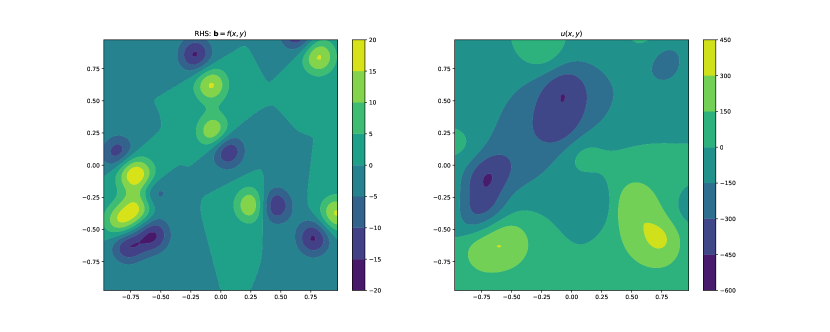
Figure 1: Example of the Poisson problems studied here – corresponding to positively and negatively charged particles randomly placed in the simulation domain. The left panel shows a random charge distribution. The right panel shows the corresponding solution to Eqs. (5) and (6).

As a starting point, we will assume that $f$ is localized (has finite support), that $u,t\in\mathbb{R}$ and that $x\in\mathbb{R}^{2}$. Discretizing Eq. (5) yields a linear problem of the form shown in Eq. (6) (where $\mathbf{A}$ is a discretization of $\nabla^{2}$ and $\mathbf{f}$ is a discretization of $f(x,t)$). In this form, the Poisson equation can be used to describe electromagnetic interactions between charged particles. An example of such a Poisson problem corresponding to randomly distributed charged particles is shown in Fig. 1. In this case, the solution to Eq. (5) corresponds to the electric potential.

In the next section we demonstrate that by going to three dimensions, Eq. (5) can be used to describe hydrodynamic flows. Consequently, accelerating an iterative linear solver as discussed earlier holds great potential for reducing the computational cost of the problems we are targeting. To this end, since Poisson-type problems form the basis of the problems we hope to solve, we establish a foundation by developing an AI-powered GMRES accelerator for the Poisson problem. In particular we focus on the Poisson problem in two-dimensions on a square domain of the form

$$\mathbf{A}u=\mathbf{f},$$ (6)

where we now specify that $A$ is the discrete Laplacian with corresponding boundary conditions, $\mathbf{f}$ corresponds to the physical forces in the problem, and $u$ is the corresponding solution. Since we plan to use deep learning to produce initial guesses $x_{0}$ to accelerate GMRES, we take a moment to examine Eq. (6) and consider how a neural network can be structured to learn a solution. Since we always have the RHS of Eq. (6) available (even if we do not yet know $u$), we structure the network such that the RHS of the Poisson problem is the neural network input and the solution is the network output. So, we seek to construct a neural network of the form

$$u=N(\mathbf{f}).$$ (7)

Since we plan to use this neural network to accelerate an ongoing simulation in real-time, efficiency with computing resources and memories are of fundamental importance: we plan to construct a neural network $N$ that is fast to train and economical with memory.

We can use the formal solution of Eq. (5) to make an informed guess about which properties of the neural network are important. If the formal solution can be represented by the network, we conjecture that there is a good chance that a network with few parameters can be trained quickly. A formal solution on some domain $\Omega$ can be expressed as

$$u=\int\limits_{\Omega}{g(\mathbf{x},\mathbf{y})f(\mathbf{y}),d\mathbf{y}},$$ (8)

where $g$ is the Green’s function. We note that for general boundary value problems the solution does not necessarily depend on the source term $f$ through a convolution if the problem is not translationally invariant since in this case the Green’s function $g$ itself may not be translationally invariant. Consequently, we should think of the solution as a non-local problem since we technically have a Fredholm integral equation of the first kind relating the solution to the RHS. Likewise, if we consider the discrete problem then we see that the solution depends on the RHS through $u=\mathbf{A}^{-1}\mathbf{f}$. As is well known, the matrix inverse of $\mathbf{A}$ is dense even if the discrete Laplacian is itself sparse. Consequently the key thing to notice is that the relationship between $\mathbf{f}$ and the solution $u$ is inherently non-local, so we must take special care of this when designing an appropriate neural network.

1.5 Relation to Fluid-Flow Problems

To illustrate how equations of the form of Eq. (5) are related to a wider class of problem, we show that simply by going to 3-dimensions, we describe a whole new class of physics: fluid flow. We introduce the vector velocity field $\mathbf{u}(x,y,z)$, the applied body forces $\mathbf{f}(x,y,z)$, and the scalar pressure field $p(x,y,z)$ (all defined on some three-dimensional domain $\Omega$). The equations for Stokes flow take the form

$$\mu\nabla^{2}\mathbf{u}-\nabla p+\mathbf{f}=0$$ (9)

$$\nabla\cdot\mathbf{u}=0,$$

where $\mu$ is the dynamic viscosity. In a number of ways, our target problem is intimately tied to the standard Poisson problem both in a mathematical sense and in the sense that numerical methods for the Poisson equations overlap with the methods for the equations for Stokes Flow. First, writing the non-divergence condition equation of Stokes flow component-wise, we have

$$\nabla^{2}{u}_{i}=\frac{1}{\mu}\left(\frac{\partial p}{\partial{{x}_{i}}}-{{{f}}_{i}}\right)\,,\,i=1,2,3.$$ (10)

Consequently, we can think of the Stokes equation in three-dimensions as essentially being three coupled scalar Poisson equations where the solutions satisfy the divergence free condition. In practice the velocity for Stokes flow (and for many fluid flow problems in general) is often related to pressure through essentially yet another Poisson equation. While the subtleties of how one relates the pressure and velocity in practice depends highly on the underlying numerical method being used (i.e projection methods, pressure correction methods, etc), in principle one arrives at a variation of the following manipulations of the governing equations in question. We illustrate this for the Stokes flow Eq. (9): by taking the divergence of the stokes flow equation in Eq. (9), making use of the incompressibility condition, and formally interchanging the divergence and Laplacian operators, we arrive at the following scalar Poisson equation for pressure

$$\nabla^{2}p=\nabla\cdot\mathbf{f}.$$ (11)

2 A Real-Time AI-Based Acceleration Algorithm

A time-dependent simulation is essentially a sequence of linear problems of the form $Ax_{i}=b_{i}$ being solved over the course of a simulation, e.g. once per time step, giving us a “time series” of length $T$. We refer to this sequence as our “simulation”. The goal here is to train a neural network $N(b)$ in real-time as linear problems are solved by GMRES($k$). This is accomplished by having the neural network provide an initial guess $N(b_{i})=x_{i}^{0}$ to GMRES($k$). The training objective is that this initial guess then improves the rate of convergence of GMRES($k$).

The data set used to train the model consists of RHS-solution pairs $\{\left(b_{i},x_{i}\right)\}$. However, unlike traditional deep learning approaches, the goal here is to train the network in real-time while data is being generated from the simulation. This naturally leads to an online supervised learning problem since at a given time $t<T$, we only have access to $N(t)$ number of $\left(b_{i},x_{i}\right)$ pairs. In the formulation presented here, at time $t<T$, the training set is $X_{t}=\{\left(b_{i},x_{i}\right)\}_{1}^{N(t)}$. In order to ensure a high-quality data set some time steps are discarded, while only “high-quality” ones are kept (this is crucial, and is discussed in a later section).

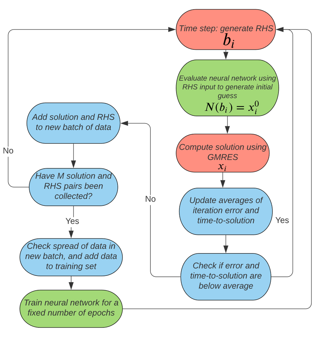
Figure 2: Experiment for accelerating GMRES with neural networks in real-time. Red boxes indicate traditional computational steps, blue boxes data collection, and green boxes indicate deep learning.

We train the neural network for a fixed number of epochs during the training phase using batched gradient descent where samples are randomly selected from $X_{t}$. When $A$ is the discrete Laplace operator, networks that are able to learn non-local relationships work especially well. Good performance was obtained with 4-6 layer CNNs with sufficiently large and dilated kernels, as well as the more sophisticated FluidNet [18] architecture described later.

Quality metrics such as the 2-norm of the GMRES residual at a particular iteration and rate-of-convergence for each guess provided by the neural network are tracked as the simulation runs. After $M$ solutions have been computed these metrics are used to decide which of the $\{\left(b_{i},x_{i}\right)\}_{1}^{N(t)}$ pairs are added to the training set for the next training phase (at some time $t^{\prime}>t$). The flow chart provided in Figure 2 outlines our real-time learning algorithm.

2.1 Neural Network Architecture

We discussed the properties necessary to capture solutions of the Poisson equation in Section 1.4. Convolutional neural networks (CNN) satisfy these and are well known to be a useful tool. However, there are two key issues that require particularly careful treatment when selecting an appropriate neural network architecture for our real-time learning context.

1. The neural network must be capable of learning non-local relationships without compressing resolution of data

2. The network should be relatively “easy” to train in the sense that the training of the network should not be on a time-scale comparable to that of the simulation

The first key issue stems from the fact that we are primarily interested in boundary value problems on finite domains that are not periodic. Even in the case of a linear problem, the relationship between the solution and the right hand side is given by an integral over the entire domain $\Omega$. Consequently, it is not surprising that in general we can expect our network to perform best if it can capture non-local information. Unfortunately, this necessity is at odds with the fact that convolutional neural network layers usually use kernels that are inherently localized. In this case, the receptive field of these networks can only grow with the depth of the neural network. While relying on an increasing network depth may not sound too taxing, it is a less than ideal solution. Deeper networks are slower to train, and the necessary depth to compensate for higher resolution problems would lead to a fairly poor trade-off in performance. Personal experience has also shown that allowing convolutions to shrink spatial resolution so that non-local features are learned, and then up-scaling to the desired output resolution yields poor results. This likely happens because important information that GMRES needs is lost as the convolutions reduce the spatial resolution.

Figure 3: We use a variation of the FluidNet pressure model of [18] in our neural network architecture shown in Figure 4. In the model used here, the number of average pooling operations depends on the problem at hand rather than being fixed.

For our test problems, we have found a particular network architecture that stands out in its ability to encode the desired non-local information while still being an all convolution architecture that does not need to rely on network depth to encode non-local information. This network is the FluidNet architecture’s pressure component from [18] – shown in Fig. 3. This network essentially works by down-sampling the input using $2^{d}$ average pooling a number of times while retaining the original and each down-sampled field. Each of these fields with different resolutions are then passed through a series of convolutional layers in parallel, and then all are up-sampled to the original resolution and summed. This sum is then passed through a series of convolutions to then produce the output field. In the architecture we use here, we essentially use a variation of this idea and increase the depth of this network by stacking residual blocks before the output layer.

The second key issue stems from the fact we are working in real-time: we must not slow down the regular (unaccelerated) code with long training times. Consequently, we are far more interested in a model that converges to a useful output quickly (and not necessarily highly accurately) than a model that slowly converges to a highly accurate output eventually. While shallower networks are known to converge to useful results quickly, their accuracy is inferior to deeper networks. Conversely, deeper networks converge slowly compared to shallow networks but are more accurate.

To balance network training speed with network depth, we have taken the approach of adaptively adding residual blocks to the output of FluidNet as the performance of the network begins to stagnate. A diagram of this approach is illustrated in Figure 4. With this approach, the relatively shallow network converges to a model that is immediately useful, and then is allowed to grow into a model that can provide outputs of improved quality. Furthermore the real-time nature of the problem restricts initial training sets to a small size. Naturally, there is a high likelihood that the state of the training set encountered initially will not be representative of all data encountered over the course of the simulation. Consequently there is a high likelihood that an initially deep network will over-fit and perform poorly as the simulation progresses. By starting with an initially shallow model, we are able to mitigate these issues.

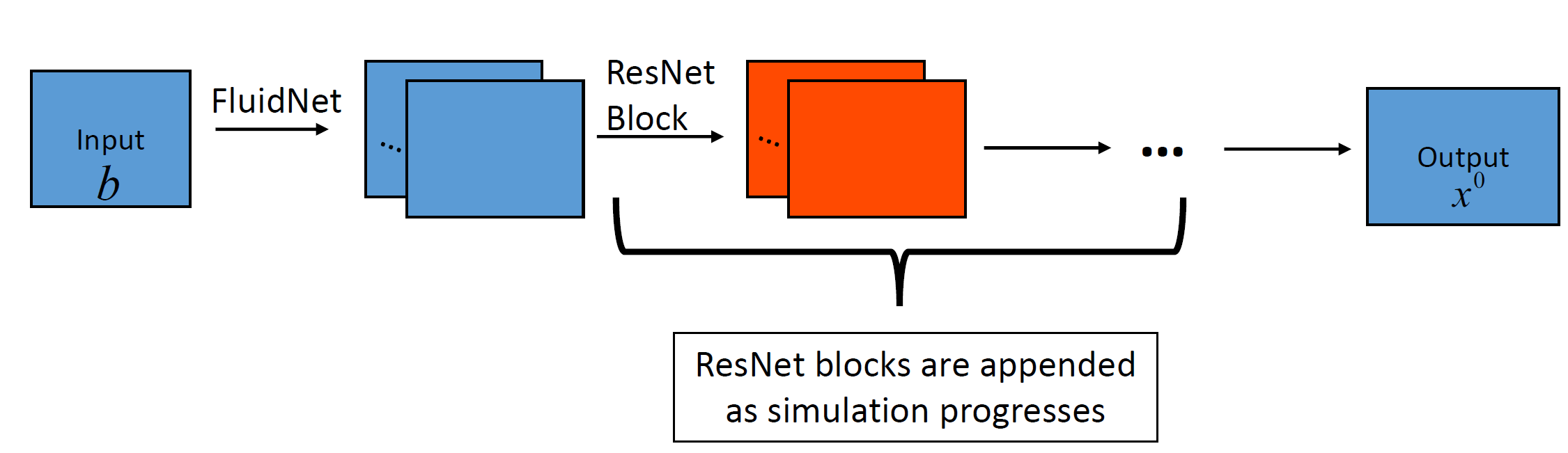
Figure 4: Resnet blocks are appended to the network before the output layer as the simulation runs. By starting with a shallow model and building up to a deeper model, we are able to benefit from fast convergence of a shallow model during early (low data) stages of a simulation and the higher accuracy of deeper models during later stages (more data) of a simulation.

2.2 Online Data Collection Process

A key part of our approach relies on collecting data from the simulation selectively. There are multiple reasons to carefully collect data selectively in this real-time context. First, since we are not working with a representative distribution of data initially – and are not necessarily guaranteed to have a representative distribution of data at any point in the simulation – we must be sure that certain types of samples are not significantly over-represented in the data set and over-fit by the model. Similarly, spurious data points can also negatively affect training and model performance significantly. Furthermore, since we cannot take an arbitrarily long time to train the model (we must keep the training time-scale relatively small compared to the simulation time scale), using a smaller representative data set rather than a massive, highly redundant data set can be beneficial.

Every simulation starts with an initial small data set of $N$ solution and RHS pairs $X_{t}=\{(b_{i},x_{i})\}_{i=0}^{N}$ by some time $\tau_{0}$ and we use a neural network $N(b)$ trained on this training set $X_{t}$ to produce initial guesses $x^{0}=N(b)$. For $t>\tau_{0}$, as the simulation progresses and before every GMRES($k$) iteration, the initial guess is generated by a forward evaluation of the neural network with the RHS as an input, i.e. we have $x^{0}=N(b)$. This guess is then used to start the GMRES($k$) iterations. Through training the neural network with a loss function that maps the RHS to solutions and the evaluation of the initial residual $x^{0}=AN(b)-b$, it is easy to determine whether this guess reduces the initial error. However, what is more important and not as easy to directly ascertain is whether this guess accelerates GMRES($k$). To this end, we keep track of two metrics and a moving average of these metrics. The first metric is the GMRES($k$) residual at the end of the first restart (i.e. the $k$th iteration) with the provided initial guess:

$$E_{k}(x^{0})=\mathbf{A}x^{k}-b.$$ (12)

The second metric is the time to reach the solution

$$\text{TOS}(x^{0})=\text{Wall-clock time taken for GMRES to converge to $x=\mathbf{A}^{-1}b$ within tolerance.}$$ (13)

Both $E(x^{0})$ and $\text{TOS}(x^{0})$ are naturally related to the rate of convergence of GMRES. To make use of these metrics, we use a moving average to set a meaningful baseline of what constitutes “good" values of $E(x^{0})$ and $\text{TOS}(x^{0})$. We define this unweighted moving average using a window that only looks at the last $p$ number of steps. Explicitly, when we have $N$ samples of some quantity $y$, we define this moving average as

$$M_{p}(\{y_{i}\}_{i=0}^{N})=\frac{y_{N-p}+\dots+y_{N}}{p}.$$ (14)

Algorithm 1 summarizes how we collect data at some time step $t=t_{n}>\tau_{0}$, we compute a solution $x^{n}$ using an initial guess $x_{n}^{0}$. Then we ccalculate $E_{k}(x_{n}^{0})$ and $\text{TOS}(x_{n}^{0})$. We also compute the moving averages of these quantities as previously defined including the most recent data $M_{p}\left(\{E_{k}(x_{i}^{0})\}\right)$ and $M_{p}\left(\{\text{TOS}(x_{i}^{0})\}\right)$. We then compare the current error and time to the mean and we check if the following two conditions hold:

$$E_{k}(x_{n}^{0})<M_{p}\left(\{E_{k}(x_{i}^{0})\}\right)$$ (15)

$$\text{TOS}(x_{n}^{0})<M_{p}\left(\{\text{TOS}(x_{i}^{0})\}\right).$$ (16)

In particular we check if the current guess provided by the network achieved a better than average error by the $k$th iteration and a better than average wall-clock time to solution. If the initial guess did meet both criteria, we simply proceed to the next time step and repeat what has been described so far. However, if the initial guess did not meet both criteria, then the model under-performed on this particular data. Consequently, the corresponding solution and RHS pair $(b_{n},x_{n})$ is then added to a set $C_{t}$ containing the candidate data points that may be added to the training set $X_{t}$. However before adding the data to $C_{t}$, the spread between $x_{n}$ and all elements of $C_{t}$ is checked. We denote the measure of spread between solutions as $d(\cdot,\cdot)$ and note the definitions depends on what is appropriate for the problem. Here, we check for sufficient orthogonality between the solution data. In particular, we check that $x_{n}$ is “sufficiently" orthogonal to all members of $C_{t}$. If this is the case, then the data point is added to $C_{t}$. Depending on whether we have encountered $f_{r}$ (the retraining frequency) data points that fail to meet our conditions, we either repeat what has been described so far, or we proceed to train the model.

Simulation has reached time $t_{n-1}$ ;

Neural network $N(b)$ has just been trained using training set $X_{t}$;

Set of candidate data pairs $C_{t}$ is empty, $N=0$;

while $N<f_{r}$ do

       $t_{n}=t_{n-1}+\Delta t_{n-1}$;

       Compute RHS $b_{n}$;

       Use Neural network $x_{n}^{0}=N(b_{n})$;

       Compute solution $x_{n}=\text{GMRES}(x_{n}^{0})$;

       Compute performance metrics $E_{k}(x_{n}^{0})$ and $\text{TOS}(x_{n}^{0})$ ;

       Compute Averages $M_{p}\left(\{E_{k}(x_{i}^{0})\}\right)$ and $M_{p}\left(\{\text{TOS}(x_{i}^{0})\}\right)$;

      

      if $E_{k}(x_{i}^{0})<M_{p}\left(\{E_{k}(x_{i}^{0})\}\right)$ and $\text{TOS}(x_{i}^{0})<M_{p}\left(\{\text{TOS}(x_{i}^{0})\}\right)$ then

             Proceed with the simulation. Set $n=n+1$ and next $\Delta t_{n-1}$

      else

             Compute $d(b_{n},b)$ for all $b$ $\in$ $C_{t}$;

             if $d(b_{n},b)$ for all $b$ is acceptable  then

                   Add $(b_{n},x_{n})$ to $C_{t}$;

             end if

            Set $N=N+1$;

             Set $n=n+1$ and next $\Delta t_{n-1}$;

       end if

      

end while

Algorithm 1 Collecting data after model has been trained

2.3 Online Training Algorithm

In our online approach, we only train at the start of the simulation or when $f_{r}$ “under-performing" data points $(b_{n},x_{n})$ are encountered. In the former case, we simply collect all data up to a reasonable point, say about $50$ time steps. Then all of these are added to the training set $X_{t}$ and the neural network is trained using the entire training set. Following this, the simulation continues while the metrics discussed above are used to judge when we add data to $C_{t}$. We then collect data as described above until $f_{r}$ new data points have been found and the model is re-trained.

In a traditional online machine learning approach, one would update the model using solely the new data from $C_{t}$. However, this typically comes at the cost of interfering with previously learned information in neural networks [19]. To mitigate this so called “catastrophic forgetting” we simultaneously train a model with data from $C_{t}$ and sampled data from the training set $X_{t}$. This way, the neural network model is not allowed to forget all previous information since it is being actively reminded of previous relationships through exposure to prior data from $X_{t}$. When training the neural network model, we train the network to minimize the objective

$$L(\tilde{x},x)=||\tilde{x}-x||_{2}^{2},$$ (17)

where $\tilde{x}$ is the initial guess provided by the network and $x^{n}$ is the solution computed by GMRES($k$). The model parameters are updated using back propagation to calculate all partial derivatives and an adaptive gradient descent method such as ADAM and Adagrad algorithms. Since the training set $X_{t}$ can become quite large, we fix the number of batch gradient descent steps so that the training time does not grow rapidly relative to the simulation time and randomly sample our training set while guaranteeing that recently collected data is used to train the model. It’s key to clarify here that minimizing the objective function is half the story, and any objective function that implicitly minimizes the initial residual of GMRES($k$) could work in principle. While minimizing the objective function coincides with our goal of minimizing the initial residual, the acceleration of GMRES($k$) is obtained through the constant monitoring of the effect of the neural network’s real-time performance in accelerating GMRES($k$). Those metrics essentially determine what data is used, and what the model should focus on learning.

3 Benchmarking an Accelerated Poisson Solver

In this section we demonstrate the viability of the concepts discussed previously. We implemented an AI-accelerated GMRES($k$) – which we call MLGMRES – by accelerating a Python implementation of the GMRES($k$) algorithm. While this implementation is obviously slower than a compiled language, the relative speedups over the original algorithm should not be affected. We work in the Python language as it allows rapid prototyping. We emphasize that none of our algorithms depend on this particular choice in languages – e.g. there has been some success applying these concepts to C++-based codes [2, 1]. However, this will not be covered here.

As a benchmark that represents realistic scientific PDE problems we solve a series of Poisson problems of the form $Ax_{i}=b_{i}$ where $A$ is the discrete Laplacian with zero-Dirichlet boundary conditions and each $i$ is a particular time-step. The $b_{i}$ used here are essentially randomly moved localized sources similar to those in Figure 5 on the square $\Omega=\left[-1,1\right]\times\left[-1,1\right]$. This is analogous to a 2-dimensional system consisting of charged particles. In a real-world setting, these particles would move according to an interaction force (e.g. $\mathbf{f}(x,x)=-\nabla u(x,y)$ where $u(x,y)$ is a solution to the Poisson equation). We move the particles randomly, making this a much harder benchmark: the test inputs are far less correlated than they would be if they were generated by physical dynamics. During our benchmarks, we find that on average 1 in 10 time steps are retained by Algorithm 1.

Our benchmarks were performed on a single Cori-GPU node at National Energy Research Scientific Computing Center (NERSC). Each node has two 20-core Intel^® Skylake^TM processors and 8 NVIDIA^® V100 GPUs. For the results presented here, we trained the model using PyTorch [20] running on 1 (out of the 8 available) GPUs. We compare against the same benchmarks running on a 10-core Intel^® Core^TM i9 desktop computer with PyTorch training on a NVIDIA^® RTX 2070. We did not see any noticeable performance difference. This gives us confidence that no specialized hardware (other than a reasonable GPU) is required to run our AI-accelerator.

3.1 Understanding the AI Accelerator through a Simplified model

We can gain a great deal of insight by considering a simpler neural network architecture. In particular if we consider a single fully connected layer as seen in Fig. 5, we can conveniently express the mapping as a matrix operation on the input. We can express this network as matrix multiplication of the form $Tb=x_{i}^{0}$. As $T$ is learned over the course of the simulation, it is reasonable to expect $AT$ to have a spectrum that clusters around the unit circle. This is particularly clear when the norm of the initial residual is considered. At the start of the GMRES($k$) iterations for a particular time-step, we have $||r_{0}||_{2}=||Ax_{i}^{0}-b||_{2}$. However, for the initial guess we use $Tb=x_{i}^{0}$. Consequently, we have $||r_{0}||=||AT-I||_{2}||b||_{2}$. So we see that for the neural network to reduce the initial residual, the spectrum of $AT$ should cluster on the unit circle. We test this idea on a simulation where we randomly move the localized source from Fig. 5 on the square with a resolution of $30\times 30$.

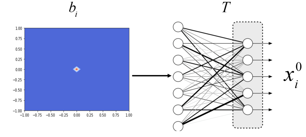
Figure 5: Simple single fully connected layer neural network model used to explore behavior of the accelerator.

In Figure 6 we show plots of the spectrum in the complex plane and the speed up provided by the neural network accelerator. The behavior observed is exactly as anticipated: we see that as we proceed in time (steps are indexed by $i$), the neural network $T$ learns a mapping such that the entire spectrum of $AT$ is moved onto the unit circle. Consequently, we see that the neural network accelerator even for this simple model is able to encode information that gives $AT$ a friendlier spectrum. This more favorable spectrum yields a lower $||r_{0}||_{2}$ and also lends some insight into why we see not just a lower initial residual, but also an improved rate of convergence. In particular, since the entire spectrum of $AT$ is eventually shifted to the unit circle, it is reasonable to conjecture that the network is encoding information that overall allows a more efficient approximation of the solution within a particular Krylov subspace.

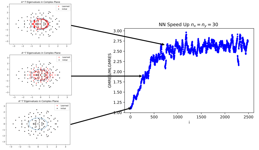
Figure 6: Spectrum of $AT$ over the course of a single simulation.

3.2 Purely Convolutional Network

In building up to the neural network architecture discussed earlier, we explored the use of sequential convolution networks where only convolutions are used. Though this architecture is not particularly sophisticated, it serves as a useful starting point for understanding how powerful the idea of deep learning based accelerators is. First, we show some results for a fixed resolution. In Fig. 7 we plot the time-to-solution (left plot) and the fifth GMRES($k$) iteration error (right) as of function of every time-step (indexed by $i$). The primary observation is that as the simulation progresses, the neural network model produces initial guesses that simultaneously improve the wall-clock time-to-solution and the fifth residual in the GMRES($k$) iteration ($||r_{5}||_{2}$). While an improved residual at the fifth iteration may be useful, it does not tell use precisely whether or not the actual rate of convergence has been improved. The speed-up we are seeing could simply be attributed to a small initial residual with zero impact on the rate of convergence. To investigate this further, we look at the GMRES($k$) residuals at each iteration for the final time step ($i=1000$). This is plotted in Fig. 8 (right panel). The blue curve corresponds to the accelerated solver. We see that the initial residual is still fairly large, roughly half of the initial residual. Consequently, improvements in the initial residual values seem to play a fairly small roll in accelerating the convergence. The second feature that differentiates the accelerated MLGMRES solver is the fact that the convergence rate is temporarily accelerated and consequently reduces the overall time-to-solution. We therefore conclude that the acceleration from our neural network “wears off” with each restart of GMRES($k$). None the less, this servers as a compelling proof of concept for this simple problem and network, since we see that we are able to accelerate GMRES.

Because we aim to be memory efficient, we next test how well a model with a fixed number of parameters scales to larger problem sizes. While keeping the number of model parameters fixed, for this simple network we dilate kernels consistently (instead of using larger kernels) with every increase in grid resolution. While we have discussed more sophisticated ways to deal with different scales, here we simply dilate kernels to get a lower bound on how robust our approach is. These results are shown in Figure 8(left panel) and Table 1. We essentially get a similar acceleration for different resolutions, and are able to keep training times relatively small compared to the time of the entire simulations.

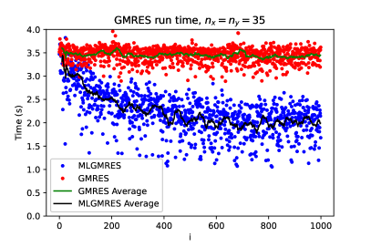
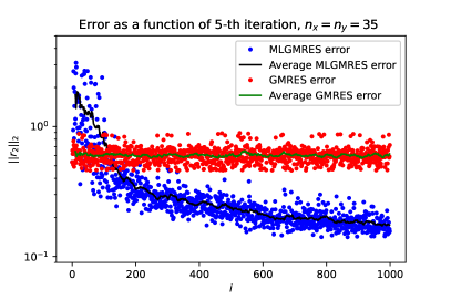
Figure 7: Left: Speed up attained by MLGMRES during the simulation. Right: Error of GMRES at the 5th iteration.

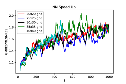
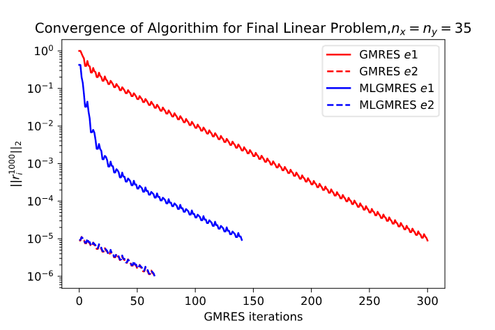
Figure 8: Left: Speed up attained by MLGMRES during the simulation for different resolutions. Right: Improvement in convergence rate of MLGMRES after 200 time steps. The final training set only contains roughly 200 data pairs. Dashed lines indicate restarts at a higher error tolerance $e_{2}$ after the first tolerance $e_{1}$ is reached. We confirm that the convergence rate for higher tolerances $e_{2}$ is not affected by the neural-network’s initial guess.

Table 1: Comparison of GMRES solver run times for different grids using the all convolution AI-acclerator

	$20\times 20$	$25\times 25$	$30\times 30$	$35\times 35$	$40\times 40$
Total GMRES Time (s)	927	1677	2718	4254	3541
Total MLGMRES Time (s)	667	1238	1971	3022	5352
Total Training Time (s)	95.1	86.2	95.2	101.5	106.1
Training Time/Total Solver Time	0.14	0.07	0.05	0.033	0.023

3.3 Neural Network Designed for Multiple Scales

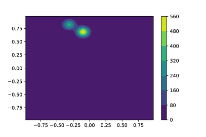
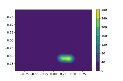
Figure 9: Examples of dipole forcing used for testing the MLGMRES (with adaptive FluidNet architecture) AI Accelerator. At every time step the dipole with two scales for each pole are randomly shifted (on the domain and relative to each-other) with different random overall scales at every time step.

While purely convolutional neural networks worked for a fairly simple RHS, they do not work quite as well on problems with multiple scales and different features. As a stepping-stone, we go from the “monopole” source term shown in Fig. 5 to “dipoles” shown in Fig. 9. For testing purposes these are not symmetric dipoles (in order to simulate systems with multiple scales). We find that purely-convolutional network architectures require more data to learn the relevant non-local relationships. To facilitate learning in these more complex scenarios, we implemented the neural network of Section 2.1. As test cases, we applied our AI-accelerator to a sequence of dipoles with the scales for each pole randomly shifted (both on the domain and relative to each-other) with different random overall scales for every single RHS. Figure 9 demonstrates some of the many possibilities seen over the course of the simulation. In Fig. 10 we see that we are able to attain a significant improvement in the GMRES time-to-solution and in the initial residual. In fact we see about an order of magnitude improvement in the fifth iteration error of GMRES (left plot in Fig. 11). This is particularly impressive given that this sequence of problems is significantly more complex than the previous example. On the right in Fig. 11 we see the GMRES error at each iteration for the final linear problem in the simulation. As before, we see that the acceleration of the solver is mostly influenced by the improved rate of convergence rather than the initial residual (which is still relatively large compared to the target tolerance).

Finally, we tested the AI-accelerator for different resolutions. Since this network architecture inherently encodes non-locality, we use the same network for each resolution. Naturally, this means that the number of model parameters is fixed while we scale the the resolution up. These results are shown on the left in Fig. 11. We see that as we increase the resolution, we get the same acceleration. So we see that even for difficult problems our network does not need to be overly complex (i.e. use an increasingly larger number of model parameters) for larger system sizes in order to accelerate the simulation. Consequently we are able to meet our efficiency targets (relatively small number of parameters and trains quickly) with this network.

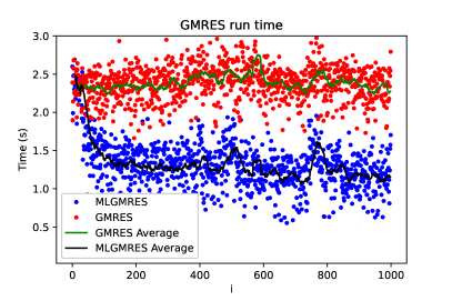
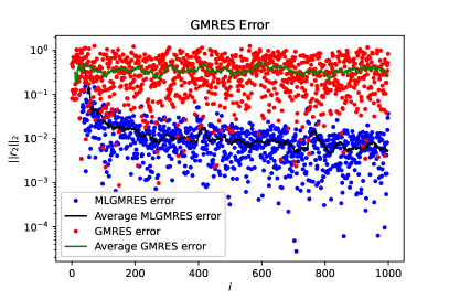
Figure 10: Left: Speed up attained by MLGMRES (with adaptive FluidNet architecture) during the simulation. Tests ran on a shared compute node. Performance variation in the un-accelerated code (red points, green line) are due to background workloads on the test system. Right: Error of GMRES at the 5th iteration during simulation.

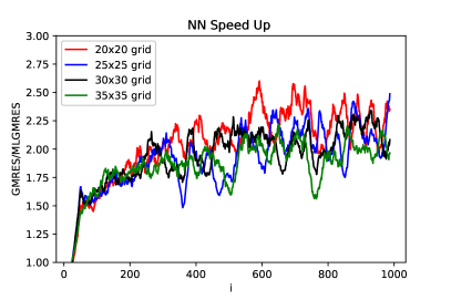
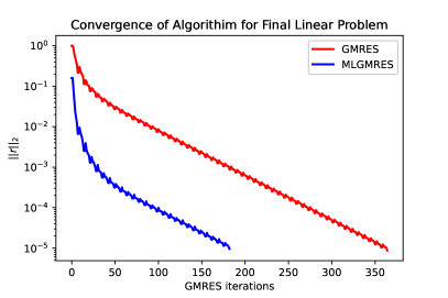
Figure 11: Left: Speed up attained by MLGMRES (with adaptive FluidNet architecture) during the simulation Right: Improvement in convergence rate of MLGMRES (with adaptive FluidNet architecture).

4 Conclusion

We have developed an in situ real-time machine learning framework that is capable of accelerating the time-to-solution of the GMRES($k$) algorithm. As demonstrated by the application in Section 3, our real-time algorithm can accelerate an iterative linear solver for the discrete Poisson equation. With relatively little input data (on average about 1 in 10 time steps yielded data that was retained by Algorithm 1), and irrespective of problem size (relative to number of network parameters) we are able to achieve a consistent 2$\times$ speedup. These results are promising for speed-up in future applications. Our approach is flexible in that the neural network model can be constructed from scratch and does not need to be pre-trained on large amounts of expensive simulation data to get a performance boost. The approach presented here only needs the desired iterative linear solver and our wrapper augments the solver calls as outlined in Fig. 2 with the user’s deep learning framework of choice. Beyond this, the methodology presented here requires no further input from the user as the simulation progresses.

5 Acknowledgements

This work was supported by the U.S. Department of Energy Office of Science, and the Computing Sciences Summer Student program at Berkeley Lab. This research used resources of the National Energy Research Scientific Computing Center (NERSC), a U.S. Department of Energy Office of Science User Facility operated under Contract No. DE-AC02-05CH11231. The authors are grateful to Stephen Whitelam, Daniel Herde, Steven Reeves, Deborah Bard, and Wibe A. de Jong for fruitful discussions.

References

- [1] Mingchao Cai, Andy Nonaka, Boyce E. Griffith, and Aleksandar Donev. Efficient variable-coefficient finite-volume stokes solvers. Communications in Computational Physics, 16:1263–1297, 2014.
- [2] Weiqun Zhang, Ann Almgren, Vince Beckner, John Bell, Johannes Blaschke, Cy Chan, Marcus Day, Brian Friesen, Kevin Gott, Daniel Graves, Max Katz, Andrew Myers, Tan Nguyen, Andrew Nonaka, Michele Rosso, Samuel Williams, and Michael Zingale. AMReX: a framework for block-structured adaptive mesh refinement. Journal of Open Source Software, 4(37):1370, May 2019.
- [3] M. Zingale, M. P. Katz, J. B. Bell, M. L. Minion, A. J. Nonaka, and W. Zhang. Improved coupling of hydrodynamics and nuclear reactions via spectral deferred corrections. The Astrophysical Journal, 886(2):105, 2019.
- [4] Michele Benzi. Preconditioning techniques for large linear systems: A survey. Journal of Computational Physics, 182(2):418–477, 2002.
- [5] Stephen Whitelam and Isaac Tamblyn. Learning to grow: Control of material self-assembly using evolutionary reinforcement learning. Physical Review E, 101(5):052604, 2020, 1912.08333.
- [6] Stephen Whitelam, Daniel Jacobson, and Isaac Tamblyn. Evolutionary reinforcement learning of dynamical large deviations. The Journal of Chemical Physics, 153(4):044113, 2020, 1909.00835.
- [7] Chris Beeler, Uladzimir Yahorau, Rory Coles, Kyle Mills, Stephen Whitelam, and Isaac Tamblyn. Optimizing thermodynamic trajectories using evolutionary reinforcement learning. arXiv preprint, 2019, 1903.08543.
- [8] Sun-Ting Tsai, En-Jui Kuo, and Pratyush Tiwary. Learning molecular dynamics with simple language model built upon long short-term memory neural network. Nature Communications, 11(1):5115, 2020.
- [9] Jaideep Pathak, Mustafa Mustafa, Karthik Kashinath, Emmanuel Motheau, Thorsten Kurth, and Marcus Day. Using Machine Learning to Augment Coarse-Grid Computational Fluid Dynamics Simulations. arXiv preprint, 2020, 2010.00072.
- [10] Matthew Hutson. From models of galaxies to atoms, simple ai shortcuts speed up simulations by billions of times. sciencemag.org, 10.1126/science.abb2769.
- [11] M. F. Kasim, D. Watson-Parris, L. Deaconu, S. Oliver, P. Hatfield, D. H. Froula, G. Gregori, M. Jarvis, S. Khatiwala, J. Korenaga, J. Topp-Mugglestone, E. Viezzer, and S. M. Vinko. Up to two billion times acceleration of scientific simulations with deep neural architecture search. arXiv preprint, 2020, 2001.08055.
- [12] Hieu Pham, Melody Guan, Barret Zoph, Quoc Le, and Jeff Dean. Efficient neural architecture search via parameters sharing. In Jennifer Dy and Andreas Krause, editors, Proceedings of the 35th International Conference on Machine Learning, volume 80 of Proceedings of Machine Learning Research, pages 4095–4104, Stockholmsmässan, Stockholm Sweden, 10–15 Jul 2018. PMLR.
- [13] Youcef Saad and Martin H. Schultz. Gmres: A generalized minimal residual algorithm for solving nonsymmetric linear systems. SIAM Journal on Scientific and Statistical Computing, 7(3):856–869, 1986, https://doi.org/10.1137/0907058.
- [14] Zhi-Hua Zhou. Machine learning challenges and impact: an interview with Thomas Dietterich. National Science Review, 5(1):54–58, 05 2017, https://academic.oup.com/nsr/article-pdf/5/1/54/31567601/nwx045.pdf.
- [15] Y. Roh, G. Heo, and S. E. Whang. A survey on data collection for machine learning: A big data - ai integration perspective. IEEE Transactions on Knowledge and Data Engineering, 33(4):1328–1347, 2021.
- [16] Lloyd Trefethen and David Bau. Numerical Linear Algebra. SIAM, 1997.
- [17] Jörg Liesen and Zdenek Strakos. Krylov Subspace Methods: Principles and Analysis. Oxford University Press, 2012.
- [18] J. Tompson, K. Schlachter, P. Sprechmann, and K. Perlin. Accelerating eulerian fluid simulation with convolutional networks. ArXiv e-prints, 2016.
- [19] German I. Parisi, Kemker Ronald, Jose L. Part, Christopher Kanan, and Stefan Wermter. Continual lifelong learning with neural networks:a review. Neural Networks, 113:54–71, 2019.
- [20] Adam Paszke, Sam Gross, Francisco Massa, Adam Lerer, James Bradbury, Gregory Chanan, Trevor Killeen, Zeming Lin, Natalia Gimelshein, Luca Antiga, Alban Desmaison, Andreas Kopf, Edward Yang, Zachary DeVito, Martin Raison, Alykhan Tejani, Sasank Chilamkurthy, Benoit Steiner, Lu Fang, Junjie Bai, and Soumith Chintala. Pytorch: An imperative style, high-performance deep learning library. In H. Wallach, H. Larochelle, A. Beygelzimer, F. d'Alché-Buc, E. Fox, and R. Garnett, editors, Advances in Neural Information Processing Systems 32, pages 8024–8035. Curran Associates, Inc., 2019.