Coherent elastic neutrino-nucleus scattering with the $\nu$BDX-DRIFT directional detector at next generation neutrino facilities

Abstract

We discuss various aspects of a neutrino physics program that can be carried out with the neutrino Beam-Dump eXperiment DRIFT ($\nu$BDX-DRIFT) detector using neutrino beams produced in next generation neutrino facilities. $\nu$BDX-DRIFT is a directional low-pressure TPC detector suitable for measurements of coherent elastic neutrino-nucleus scattering (CE$\nu$NS) using a variety of gaseous target materials which include carbon disulfide, carbon tetrafluoride and tetraethyllead, among others. The neutrino physics program includes standard model (SM) measurements and beyond the standard model (BSM) physics searches. Focusing on the Long Baseline Neutrino Facility (LBNF) beamline at Fermilab, we first discuss basic features of the detector and estimate backgrounds, including beam-induced neutron backgrounds. We then quantify the CE$\nu$NS signal in the different target materials and study the sensitivity of $\nu$BDX-DRIFT to measurements of the weak mixing angle and neutron density distributions. We consider as well prospects for new physics searches, in particular sensitivities to effective neutrino non-standard interactions.

I Introduction

Coherent elastic neutrino-nucleus scattering (CE$\nu$NS) is a process in which neutrinos scatter on a nucleus which acts as a single particle. Within the Standard Model (SM), CE$\nu$NS is fundamentally described by the neutral current interaction of neutrinos and quarks, and due to the nature of SM couplings it is approximately proportional to the neutron number squared Freedman (1974). Following years of experimental efforts, the COHERENT collaboration has established the first detection of CE$\nu$NS using a stopped-pion source with both a CsI[Na] scintillating crystal detector Akimov et al. (2017) and single-phase liquid argon target Akimov et al. (2021).

There are many proposed experimental ideas to follow up on the detection of CE$\nu$NS, using for example reactor Wong et al. (2007); Billard et al. (2017); Agnolet et al. (2017); Ko et al. (2017); Aguilar-Arevalo et al. (2019); Angloher et al. (2019); Akimov et al. (2020a); Fernandez-Moroni et al. (2020), SNS Akimov et al. (2018); Baxter et al. (2020), and ⁵¹Cr sources Bellenghi et al. (2019). The COHERENT data and these future detections provide an exciting new method to study beyond the SM (BSM) physics through the neutrino sector, as well as provide a new probe of nuclear properties.

Since the power of CE$\nu$NS as a new physics probe is just now being realized, it is important to identify new ways to exploit CE$\nu$NS in future experiments. In this paper, we propose a new idea to study CE$\nu$NS with the neutrino Beam-Dump eXperiment Directional Identification From Tracks ($\nu$BDX-DRIFT) detector using neutrino beams at next generation neutrino experiments. For concreteness we focus on the Long Baseline Neutrino Facility (LBNF) beamline at Fermilab Strait et al. (2016). As we show, this experimental setup is unique relative to on-going CE$\nu$NS experiments, for two primary reasons. First, the LBNF beam neutrinos are produced at a characteristic energy scale different than neutrinos from reactor or SNS sources. This provides an important new, third energy scale at which the CE$\nu$NS cross section can be studied. Second, our detector has directional sensitivity, which improves background discrimination and signal extraction. Previous studies have shown how directional sensitivity improves sensitivity for BSM searches Abdullah et al. (2020).

This paper is organized as follows. In Section II we discuss the basic features of the $\nu$BDX-DRIFT detector setup that we are considering. In Section III we discuss the expected CE$\nu$NS signal at $\nu$BDX-DRIFT. In Section IVA, we investigate the backgrounds at $\nu$BDX-DRIFT and in Section IVB, we show the aspects of SM and BSM physics that can be studied using $\nu$BDX-DRIFT. In Section V we present our conclusions.

II $\nu$BDX-DRIFT: Basic detector features

As discussed in Snowden-Ifft et al. (2019), a BDX-DRIFT detector, with its novel directional and background rejection capabilities, is ideally suited to search for elastic, coherent, low-energy, nuclear-recoils from light dark matter (DM). A sketch of a BDX-DRIFT detector is shown in Figure 1. The readouts on either end couple to two back-to-back drift volumes filled with a nominal mixture of 40 Torr CS₂ and 1 Torr O₂ and placed into a neutrino beam, as shown. The use of the electronegative gas CS₂ allows for the ionization to be transported through the gas with only thermal diffusion which largely preserves the shape of the track Snowden-Ifft and Gauvreau (2013). CS₂ releases the electron near the gain element allowing for normal electron avalanche to occur at the readout Snowden-Ifft and Gauvreau (2013). The addition of O₂ to the gas mixture allows for the distance between the recoil and the detector to be measured without a $t_{0}$ (time of creation of the ionization) Battat et al. (2017); Snowden-Ifft (2014); Battat et al. (2015) eliminating, with side-vetoes, prodigious backgrounds from the edges of the fiducial volume. Because of the prevalence of S in the gas and the $Z^{2}$ dependence for coherent, elastic, low-energy scattering, Snowden-Ifft et al. (2019) the recoils would be predominantly S nuclei. With a theshold of 20 keV the S recoils would be scattered within one degree of perpendicular to the beam line due to extremely low-momentum transfer, scattering kinematics. The signature of these interactions, therefore, would be a population of events with ionization parallel to the detector readout planes.

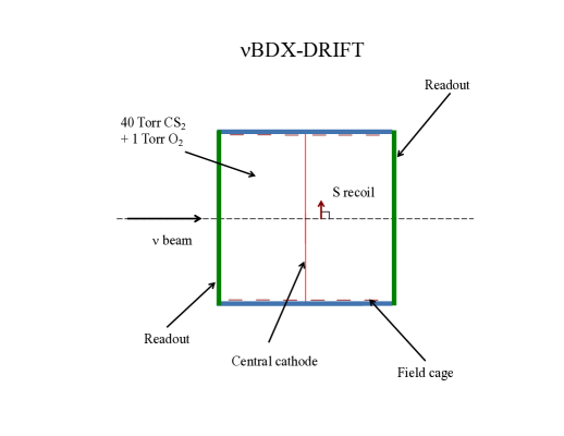
Figure 1: A sketch of the $\nu$BDX-DRIFT detector.

Here we consider deploying a BDX-DRIFT detector in a neutrino beam of a next generation neutrino facility, which for definitiveness we take to be the LBNF beamline at Fermilab. As discussed below CE$\nu$NS will produce low-energy nuclear recoils in the fiducial volume of a $\nu$BDX-DRIFT detector. To optimize the detector for CE$\nu$NS detection various gas mixtures and pressures are considered.

III CE$\nu$NS in $\nu$BDX-DRIFT

When the neutrino-nucleus exchanged momentum is small enough ($q\lesssim 200\,$MeV) the individual nucleon amplitudes sum up coherently, resulting in a coherent enhancement of the neutrino-nucleus cross section Freedman (1974). So rather than scattering off nucleons the neutrino scatters off the entire nucleus. This constraint on $q$ translates into an upper limit on the neutrino energy $E_{\nu}\lesssim 100\,$MeV, which in turn “selects” the neutrino sources capable of inducing CE$\nu$NS. At the laboratory level, reactor neutrinos with $E_{\nu}\lesssim 9\,$MeV dominate the low energy window, while stopped-pion sources with $E_{\nu}<m_{\mu}/2$ the intermediate energy window. Fig. 2 shows the different energy domains at which CE$\nu$NS can be induced. At the astrophysical level CE$\nu$NS can be instead induced by solar, supernova and atmospheric neutrinos in the low, intermediate and “high” energy windows, respectively.

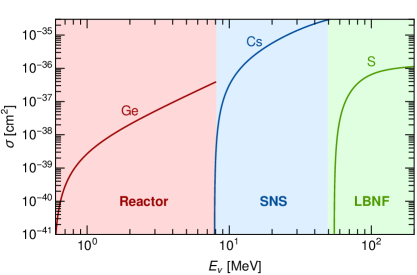
Figure 2: CE$\nu$NS total cross section as a function of incoming neutrino energy for reactor neutrinos, spallation neutron source (SNS) neutrinos and the LBNF beamline. Cross sections are calculated for representative nuclides of the technologies used in each case: germanium (reactor), cesium (SNS) and sulfur (LBNF). This graph shows the different energy domains at which a significant CE$\nu$NS signal can be induced.

Using laboratory-based sources, CE$\nu$NS has been measured by the COHERENT collaboration with CsI[Na] and LAr detectors Akimov et al. (2017, 2020b). And measurements using reactor neutrino sources are expected in the near-future Agnolet et al. (2017); Aguilar-Arevalo et al. (2019); Strauss et al. (2017). The high-energy window however has been rarely discussed and experiments covering that window have been so far not considered. One of the reasons is probably related with the conditions that should be minimally satisfied for an experiment to cover that energy range: (i) The low-energy tail of the neutrino spectrum should provide a sufficiently large neutrino flux, (ii) the detector should be sensitive to small energy depositions and (iii) backgrounds need to be sufficiently small to observe the signal. The LBNF beamline combined with the $\nu$BDX-DRIFT detector satisfy these three criteria, as we will now demonstrate.

Accounting for the neutron and proton distributions independently, i.e. assuming that their root-mean-square (rms) radii are different $\langle r^{2}_{n}\rangle\neq\langle r^{2}_{p}\rangle$, the SM CE$\nu$NS differential cross section reads Freedman (1974); Freedman et al. (1977)

$$\frac{d\sigma}{dE_{r}}=\frac{m_{N}G_{F}^{2}}{2\pi}\left(2-\frac{E_{r}m_{N}}{E_{\nu}^{2}}\right)Q^{2}_{W}\ ,$$ (1)

where the coherent weak charge quantifies the $Z$-nucleus vector coupling, namely

$$Q_{W}^{2}=\left[Ng_{V}^{n}F_{N}(q)+Zg_{V}^{p}F_{Z}(q)\right]^{2}\ .$$ (2)

The proton and neutron charges are determined by the up and down quark weak charges and read $g_{V}^{n}=-1/2$ and $g_{V}^{p}=1/2-2\sin^{2}\theta_{W}$. In the Born approximation the nuclear form factors are obtained from the Fourier transform of the neutron and proton density distributions. The properties of these distributions are captured by different parametrizations, which define different form factors. For all our calculations we use the one provided by the Helm model Helm (1956), apart from Section IV.2.2 where we will as well consider those given by the symmetrized Fermi distribution function and the Klein-Nystrand approach Sprung and Martorell (1997); Klein and Nystrand (1999) (see that Section for details). Note that the dependence that the signal has on the form factor choice is a source for the signal uncertainty.

In almost all analyses $\langle r^{2}_{n}\rangle=\langle r^{2}_{p}\rangle$, and so the form factor factorizes. That approximation is good enough unless one is concerned about percent effects Aristizabal Sierra et al. (2019a); Hoferichter et al. (2020), $\langle r^{2}_{p}\rangle$ values for $Z$ up to 96 are known at the part per thousand level through elastic electron-nucleus scattering Angeli and Marinova (2013). In that limit one can readily see that the differential cross section is enhanced by the number of neutrons ($N^{2}$) of the target material involved, a manifestation of the coherent sum of the individual nucleon amplitudes. In what follows all our analyses will be done in that limit, the exception being Sec. IV.2.2.

The differential event rate (events/year/keV) follows from a convolution of the CE$\nu$NS differential cross section and the neutrino spectral function properly normalized

$$\frac{dR}{dE_{r}}=V_{\text{det}}\,\rho(P)\frac{N_{A}}{m_{\text{molar}}}\int_{E_{\nu}^{\text{min}}}^{E_{\nu}^{\text{max}}}\,\frac{d\sigma}{dE_{r}}\,\frac{d\Phi}{dE_{\nu}}dE_{\nu}\ .$$ (3)

Here $E_{\nu}^{\text{min}}=\sqrt{m_{N}E_{r}/2}$. The first two factors define the detector mass $m_{\text{det}}=V_{\text{det}}\,\rho(P)$, where $\rho(P)$ corresponds to the target material density which depends on detector pressure at fixed room temperature, $T=293\,$K. Assuming an ideal gas it reads,

$$\rho=5.5\times 10^{-5}\times\left(\frac{m_{\text{molar}}}{\text{g}/\text{mol}}\right)\left(\frac{P}{\text{Torr}}\right)\frac{\text{kg}}{\text{m}^{3}}\ .$$ (4)

Pressure and recoil energy threshold are related and their dependence varies with target material. For the isotopes considered here, assuming CS₂ to be the dominant gas, we have:

$$E_{r}^{\text{th}}(\text{Nuc}_{i})=f_{i}\,\left(\frac{P}{40~{}\text{Torr}}\right)\,\text{keV}\ ,$$ (5)

with $f_{i}=\{2,7.5,13,20,69\}$ for $\text{Nuc}_{i}=\{\text{H},\text{C},\text{F},\text{S},\text{Pb}\}$ Battat et al. (2017); Burgos et al. (2007). For the neutrino spectrum (and normalization) we use the DUNE near detector flux prediction for three different positions (on-axis and off-axis 9 m ($0.5^{\circ}$ off-axis) and 33 m ($2.0^{\circ}$ off-axis)) Abi et al. (2020). Fig. 3 shows the corresponding fluxes (left graph) along with the low energy region relevant for CE$\nu$NS (right graph).

With these results we are now in a position to calculate the CE$\nu$NS event yield for potential different target materials (compounds): carbon disulfide, carbon tetrafluoride and tetraethyllead as a function of pressure (threshold). We start with carbon disulfide and assume the following detector configuration/operation values: $V_{\text{det}}=10\,\text{m}^{3}$ and seven-year data taking. Results for smaller/larger detector volumes as well as for smaller/larger operation times follow from an overall scaling of the results presented here, provided the assumption of a pointlike detector is kept.

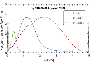
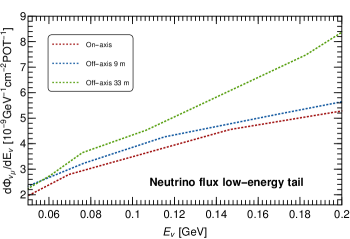
Figure 3: Left graph: Neutrino flux at the $\nu$BDX-DRIFT location ($L_{\text{LBNF}}=574\,$m) for three positions: on-axis and off-axis 9 m and 33 m ($0.5^{\circ}$ and $2.0^{\circ}$ off-axis) Abi et al. (2020). Right graph: Low-energy tail of the neutrino spectra, relevant for CE$\nu$NS, for the three positions considered in the left graph. See discussion in Section III for details.

Left graph in Fig. 4 shows the CE$\nu$NS event rate for CS₂, carbon and sulfur independently displayed. The result is obtained by assuming the on-axis neutrino flux configuration. One can see that up to 700 Torr the event rate is dominated by the sulfur contribution, point at which carbon overtakes the event rate with a somewhat degraded contribution. The individual behavior of each contribution can be readily understood as follows. At low recoil energies the event rate is rather flat but pressure is low, thus the suppression of both contributions in that region is due to low pressure. As pressure increases, $m_{\text{det}}$ increases, as do the carbon and sulfur event rates. There is a pressure, however, for which the processes start losing coherence and so the event rates start decreasing accordingly (variations in pressure translate into variations in recoil energy threshold according to Eq. (5)). For sulfur it happens at lower pressures than for carbon, as expected given that sulfur is a heavier nucleus. For CS₂ then it is clear that the optimal pressure is set at about 400 Torr (exactly at 411 Torr), a value that corresponds to $E_{r}^{\text{th}}\simeq 77.1\,$keV for carbon and to $E_{r}^{\text{th}}=205.5\,$keV for sulfur, according to Eq. (5). In summary, at the optimum pressure and corresponding threshold, for CS₂ the number of CE$\nu$NS events for a 7-year 10 cubic-meter exposure is 367.

Although rather energetic, it is clear that the LBNF beamline can induce CE$\nu$NS and that the process can be measured, provided the detector is sensitive to low recoil energies. The details of how CE$\nu$NS proceeds are as follows. The low-energy tail of the neutrino spectrum (on-axis) extends down to energies of order 50 MeV or so, as can be seen in the right graph in Fig. 3. From that energy and up to those where coherence is lost, the neutrino flux will induce a sizable number of CE$\nu$NS events. Taking the recoil energy at which $F^{2}(E_{r})$ decreases from $1$ to $0.1$ as the energy at which coherence is lost (above those energies the nuclear form factor decreases rapidly and enters a dip, regardless of the nuclei), $E_{\nu}$ can be determined with the aid of $E_{\nu}=\sqrt{2m_{N}E_{r}}$. Since for sulfur (carbon) we found $E_{r}^{\text{S}}\simeq 370\,$keV ($E_{r}^{\text{C}}\simeq 1800\,$keV), we get $E_{\nu}^{\text{S}}\simeq 150\,$MeV ($E_{\nu}^{\text{C}}\simeq 200\,$MeV). Numerically we have checked that the event yield changes only in one part per thousand when increasing $E_{r}^{\text{max}}$ to values for which $E_{\nu}>200\,$MeV.

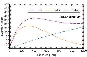
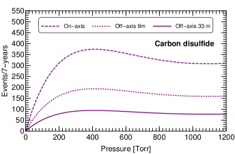
Figure 4: Left graph: CE$\nu$NS event yield for carbon dioxide in terms of pressure assuming a ten-cubic meter detector volume operating at room temperature during a 7-years data taking period. Right graph: CE$\nu$NS event yield for different detector position configurations: on-axis and off-axis $9\,$m and $33\,$m ($0.5^{\circ}$ and $2.0^{\circ}$ off-axis).

The number of muon neutrinos per year per $\text{cm}^{2}$ delivered by the LBNF beamline in the on-axis configuration and the full energy range, $[0.5,5\times 10^{3}]\,$ MeV, is $1.1\times 10^{14}$. For the energy range that matters for CE$\nu$NS this number is instead $10^{12}$. There are about two orders of magnitude less neutrinos for CE$\nu$NS than e.g. for elastic neutrino-electron scattering. However, the flux depletion is somewhat compensated by the $N^{2}$ enhancement of the CE$\nu$NS cross sections, which for sulfur (carbon) amounts to $256$ ($36$). Thus, although fewer neutrinos are available for CE$\nu$NS, the large size of the corresponding cross section leads to a sizable number of events even for neutrino energies far above those of spallation neutron source neutrinos.

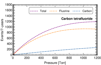
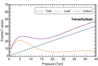
Figure 5: Left graph: CE$\nu$NS event rates as a function of pressure for carbon tetrafluorine ($\text{CF}_{4}$) assuming a ten-cubic meter detector volume, operation at room temperature and on-axis neutrino flux configuration. The calculation assumes the bulk of the gas is filled with $\text{CF}_{4}$. Right graph: Same as left graph but for tetraethyllead ($\text{C}_{8}\text{H}_{20}\text{Pb}$). Hydrogen contributes to the signal at the per mille level and so its contribution is not displayed. In contrast to $\text{CF}_{4}$, in this case a concentration of 2.3:1 of carbon disulfide and tetraethyllead has been assumed.

From Fig. 3, and as expected, it is clear that the number of neutrinos decreases as one moves off the axis. For the configurations shown there we calculate: and $n_{\nu}(33\text{m})=9.3\times 10^{12}\,\nu_{\mu}/\text{year}/\text{cm}^{2}$ (integrating over the full neutrino energy range, $[5\times 10^{-2},5]\,$GeV). So the CE$\nu$NS event rates for these off-axis configurations are depleted, although as a function of pressure they keep the same behavior, as can be seen in the right graph in Fig. 4. Note that off-axis configurations, in particular that at $33\,\text{m}$, can potentially be ideal for light DM searches since they lead to a suppression of neutrino (or neutrino-related) backgrounds Aristizabal Sierra et al. (2021).

$\nu$BDX-DRIFT is suitable for other target materials as well, so we have investigated the behavior of their event rates. The left graph in Fig. 5 shows the result for carbon tetrafluoride (CF₄), while the right graph for tetraethyllead ($\text{C}_{8}\text{H}_{20}\text{Pb}$). For the results in the left graph we have assumed the bulk of the gas is filled with $\text{CF}_{4}$, i.e. 100% of the fiducial volume is filled with $\text{CF}_{4}$. Note that this a rather good approximation given that $\text{CS}_{2}$ and $\text{CF}_{4}$ have about the same number of electrons per molecule. For the results in the right graph we have instead taken a CS₂:$\text{C}_{8}\text{H}_{20}\text{Pb}$ concentration of 2.3:1. As we will discuss in Section IV.2.2, these compounds are particularly useful for measurements of the root-mean-square (rms) radius of the neutron distributions of carbon, fluorine and lead.

From these results one can see that for carbon tetrafluoride the signal is dominated by fluorine, with subdominant contributions from carbon. Fluorine being a slightly heavier nuclei has intrinsically a larger cross section, with an enhancement factor of order $(N_{\text{F}}/N_{\text{C}})^{2}=100/36\simeq 2.8$. In addition the carbon-to-fluorine ratio of the compound implies an extra factor 4 for the fluorine contribution. One can see as well that up to 1200 Torr the signal increases. For analyses in $\text{CF}_{4}$ we take the CE$\nu$NS signal at $400\,$Torr, for which we get 808 events/7-years.

In terms of pressure, tetraethyllead behaves rather differently. The signal is dominated by lead up to 12 Torr or so. At that point the carbon contribution kicks in and dominates the signal, particularly at high pressure. Hydrogen contributes to the signal at the per mille level, despite being enhanced by a factor 20 from the molecular composition. This is expected, in contrast to the carbon and lead cross sections the hydrogen contribution is not enhanced. The behavior of the lead and carbon contributions can be readily understood. Relative to lead the carbon coherence enhancement factor is small $(N_{\text{C}}/N_{\text{Pb}})^{2}\simeq 2.3\times 10^{-3}$. However, lead loses coherence at rather low pressures and so the difference is mitigated. One can see that for $P<12\,$Torr carbon contributes at the percent level.

The pressure at which the lead signal peaks is relevant if one is interested in lead related quantities. That pressure corresponds to $6.4\,$Torr, for which carbon contributes about $25\%$ of the total signal. At that pressure the signal amounts to 26 events/7-years, with the contribution from lead (carbon) equal to 19.2 events/7-years (6.7 events/7-years). Thus for such measurements one will need as well to distinguish recoils in lead from those in carbon, something that seems viable given that the range of C for a given ionization should be much larger than for Pb.

IV $\nu$BDX-DRIFT physics potential beyond CE$\nu$NS measurements

After discussing CE$\nu$NS measurements with the $\nu$BDX-DRIFT detector, we now proceed with a discussion of possible problematic backgrounds as well as studies that can be carried out with the detector. For the latter we split the discussion in measurements of SM quantities and BSM searches. We would like to stress that although BSM searches at $\nu$BDX-DRIFT include those for light DM, here we limit our discussion to the case of new interactions in the neutrino sector that can potentially affect the CE$\nu$NS event spectrum. The discussion of light DM will be presented elsewhere Aristizabal Sierra et al. (2021).

IV.1 Estimation of backgrounds at $\nu$BDX-DRIFT

DRIFT detectors have been shown to be insensitive to all types of ionizing radiation except nuclear recoils after analysis cuts have been applied with minimal loss of sensitivity Battat et al. (2017). The most recent results from the Boulby Mine show no nuclear recoil events in the fiducial volume in 55 days of running Battat et al. (2017). These results have been extended now to 150 days of running Snowden-Ifft (2021a). Furthermore DRIFT detectors have been run on the surface and only been found to be sensitive to cosmic ray neutrons Snowden-Ifft (2021b). The DUNE near detector site is at a depth of 60 m and any possibility of nuclear recoils induced from cosmic rays at this shallower depth than the Boulby Mine would be vetoed by timing cuts. The several second cycle time of the LBNF beam is ideally suited to the slow drift speed of a DRIFT detector. Thus beam-unrelated backgrounds will not be a limitation at LBNF.

Beam-related backgrounds are possibly concerning. In this section we address the most worrisome beam-related background, neutrino-induced neutrons (NINs). The neutrino beam interacts not only with the target material but with the vessel walls as well. In that process, some neutrinos can interact with the nucleons of the vacuum vessel to produce neutrons, which could enter the active detector volume and produce a background of low-energy nuclear-recoils. Depending on the neutrino beam energy distribution, and the vacuum vessel material, different processes are to be considered. For an iron vessel (mostly ⁵⁶Fe) and $E_{\nu}\lesssim 0.1\,$GeV, the incoming neutrino can strip off a neutron from ⁵⁶Fe, thus inducing the stripping reaction ${}^{56}\text{Fe}+\nu_{\mu}\to n+^{55}\text{Fe}+\nu_{\mu}$. The total cross section for this processes ranges from $10^{-42}\,\text{cm}^{2}$ to $10^{-41}\,\text{cm}^{2}$, and dominates NIN production in that neutrino energy regime Kolbe and Langanke (2001).

For neutrino energies above $\sim 0.1\,$GeV other processes can dominate. The on-axis LBNF spectrum peaks within 2-3 GeV and extends up to energies of order 5 GeV (see Fig. 3). Thus, although LBNF neutrinos trigger iron stripping reactions, their rate is small compared to neutrino processes which open up as soon as $E_{\nu}\gtrsim 0.1\,$GeV, namely: elastic scattering (E); quasielastic scattering (QE); resonant single pion production (RES); deep inelastic scattering (DIS). Of course, not all these processes produce final state neutrons, only E and RES do. For initial-state neutrinos, RES processes are Formaggio and Zeller (2012)

CC: $$\nu_{\mu}+p\to\mu^{-}+p+\pi^{+}\ , \quad\nu_{\mu}+n\to\mu^{-}+p+\pi^{0}\ ,$$

$$\nu_{\mu}+n\to\mu^{-}+n+\pi^{+}\ ,$$ (6)

NC: $$\nu_{\mu}+p\to\nu_{\mu}+p+\pi^{0}\ , \quad\nu_{\mu}+p\to\nu_{\mu}+n+\pi^{+}\ ,$$

$$\nu_{\mu}+n\to\nu_{\mu}+n+\pi^{0}\ , \nu_{\mu}+n\to\nu_{\mu}+p+\pi^{-}\ .$$ (7)

Thus, only three out of seven involve final-state neutrons which could give recoils mimicking the signal. As can be seen in Eq. (IV.1) RES CC processes produce as well charged products which would likely be picked up in the fiducial volume and so vetoed, but are included here for a generous estimate of the backgrounds. The protons produced by the other processes could produce recoils but are charged and so could be similarly vetoed. Pions are either charged and so can be vetoed or uncharged and decaying so quickly to photons that they cannot produce recoils. So we then estimate the $\nu\to n$ total cross section according to

$$\sigma_{\text{NIN}}=\sigma_{\text{E}}+\frac{3}{7}\sigma_{\text{RES}}\ ,$$ (8)

where we assume that the seven RES processes contribute equally to the RES total cross section. Fixing $E_{\nu}=3\,$GeV and using the SM prediction for the total neutrino cross section at these energies Formaggio and Zeller (2012) one then gets $\sigma_{\text{NIN}}=6.2\times 10^{-39}\,\text{cm}^{2}$.

With the relevant cross section estimated we can now calculate the expected number of NIN events. Assuming the full $\nu$BDX-DRIFT detector will be made of $N_{\text{modules}}$ $\nu$BDX-DRIFT modules each having $1\,\text{m}^{3}$ fiducial volumes surrounded by vacuum vessels $150\,\text{cm}$ on a side we then write the number of NIN per cycle as follows

$$\frac{N_{\text{NIN}}}{\text{cycle}}= 3.0\cdot 10^{-4}\left(\frac{\mathcal{F}}{3}\right)\left(\frac{n_{\text{Fe}}}{2.4\cdot 10^{24}/\text{cm}^{3}}\right)\left(\frac{n_{\nu}}{772640/\text{cm}^{2}}\right)$$

$$\left(\frac{A}{22500\,\text{cm}^{2}}\right)\left(\frac{t}{1\,\text{cm}}\right)\left(\frac{\sigma_{\text{NIN}}}{6.2\cdot 10^{-39}\,\text{cm}^{2}}\right)\,N_{\text{modules}}\ .$$ (9)

Here $\mathcal{F}$ refers to the number of faces, $n_{\text{Fe}}$ to the iron neutron density, $n_{\nu}$ to the number of neutrinos per cycle, $A$ to the area of each face, and $t$ to the vessel wall thickness. We assume only 3 detector faces (front and half of the four lateral faces) are relevant because of forward scattering of the neutrons, while for $n_{\nu}$ we take the on-axis neutrino flux in Fig. 3 rescaled by $n_{\text{POT}}/\text{cycle}=7.5\times 10^{13}$ Strait et al. (2016). Taking 1.0 second as a representative LBNF cycle time (LBNF extractions oscillate in the range 0.7-1.2 s Strait et al. (2016)), a 10 cubic-meter detector and a data-taking period of 7 years, one gets $N_{\text{NIN}}/\text{7-\text{years}}\simeq 6.56\times 10^{5}$.

Given the LBNF beamline energy spectrum and the final-state particles in the processes of interest (E and RES), NINs are order GeV. The detection probability $\mathcal{P}$ for those GeV neutrons at $\nu$BDX-DRIFT operating with 100% of the fiducial volume filled with CS₂ at $400\,\text{Torr}$ has been determined by a GEANT4 Agostinelli et al. (2003) simulation benchmarked to neutron-induce nuclear-recoil data Battat et al. (2017). The result is $\mathcal{P}=2.5\times 10^{-5}$. With this number we then estimate the number of effective NIN events over the relevant time period and for 10 modules to be

$$\frac{N_{\text{NIN}}^{\text{eff}}}{\text{7-years}}= \mathcal{P}\times\left(\frac{N_{\text{NIN}}}{\text{7-\text{years}}}\right)$$

$$= 16.0\ .$$ (10)

From the CS₂ calculation represented in the left graph of Fig. 4 we expect 367 CE$\nu$NS events above threshold for the same exposure. This means that the signal-to-background (NIN) ratio is about 23, a number comparable to what the COHERENT collaboration found for the same type of events (47) Akimov et al. (2017). Following this analysis, our conclusion is that the NIN background contamination of the CE$\nu$NS signal is small for all possible realistic detector configurations.

NINs produced in the surrounding environment are less concerning as they can be shielded against either passively or actively, e.g. Westerdale et al. (2016).

IV.2 SM and BSM studies with the $\nu$BDX-DRIFT detector

Measurements of the CE$\nu$NS event spectrum can be used to extract information on the weak mixing angle as well as on the rms radii of neutron distributions. Using COHERENT CsI[Na] and LAr data this approach has been used for $\sin^{2}\theta_{W}$ Papoulias and Kosmas (2018); Miranda et al. (2020). It has been used as well in forecasts of near-future reactor-based CE$\nu$NS data Canas et al. (2016); Cañas et al. (2018). These analyses provide relevant information for this SM parameter at renormalization scales of order $\langle q\rangle=\mu\simeq 10^{-2}\,$GeV and $\mu\simeq 10^{-3}\,$GeV, respectively. An analysis complementary to CE$\nu$NS-related experiments has been as well discussed using elastic neutrino-electron scattering with the DUNE near detector de Gouvea et al. (2020). This measurement will provide information at $\mu\simeq 6\times 10^{-2}\,$GeV, with higher precision that what has been so far obtained by COHERENT and comparable to what will be obtained with e.g. MINER and CONNIE.

Measurements of the rms radii of neutron distributions can be as well performed through the observation of the CE$\nu$NS process. From Eq. (1) one can see that information on the CE$\nu$NS event spectrum can be translated into limits on $r_{\text{rms}}^{n}=\sqrt{\langle r^{2}_{n}\rangle}$, encoded in $F_{N}(q)$. Analyses of these type have been carried out using COHERENT CsI[Na] data in the limit $r_{\text{rms}}^{n}|_{\text{Cs}}=r_{\text{rms}}^{n}|_{\text{I}}$, for which Ref. Cadeddu et al. (2018) found the 1$\sigma$ result $r_{\text{rms}}^{n}|_{\text{Cs,I}}=5.5^{+0.9}_{-1.1}\,$fm. Later on using the LAr data release a similar analysis found the $90\%$ CL upper limit $r_{\text{rms}}^{n}<4.33\,$fm Miranda et al. (2020), a value which mainly applies to ⁴⁰Ar given its natural abundance. Forecasts of neutron distributions measurements using CE$\nu$NS data have been presented in Ref. Coloma et al. (2020a).

In addition to SM measurements, CE$\nu$NS can be used as a probe for new physics searches. Using COHERENT data, various BSM scenarios have been studied. They include neutrino non-standard interactions (NSIs) and neutrino generalized interactions, light vector and scalar mediators interactions, sterile neutrinos and neutrino electromagnetic properties (see e.g. Liao and Marfatia (2017); Coloma et al. (2017a, 2020b); Farzan et al. (2018); Aristizabal Sierra et al. (2019b, 2018a); Papoulias and Kosmas (2018); Miranda et al. (2019); Papoulias (2020); Miranda et al. (2020); Dutta et al. (2019)). To illustrate the capabilities of the $\nu$BDX-DRIFT detector and as a proof of principle, here we focus on NSI scenarios. Given the ingoing neutrino flavor the couplings that can be proved are $\epsilon_{\mu e}$, $\epsilon_{\mu\mu}$ and $\epsilon_{\mu\tau}$ (see Section IV.2.3 for details). We then focus on these couplings and consider—for simplicity—a single-parameter analysis.

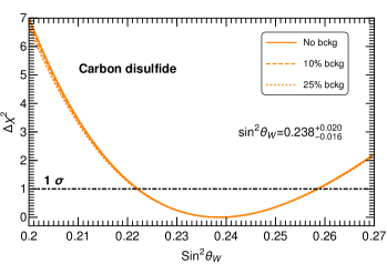
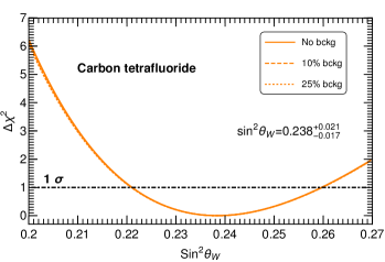
Figure 6: Left graph: Chi-square distribution for $\sin^{2}\theta_{W}$ assuming a ten-cubic meter detector volume, 7-years data taking and 100% detector efficiency. The calculation has been done assuming the bulk of the gas is filled with CS₂ under three background hypotheses: A free background measurement and $10\%$ and $25\%$ of the measured signal, assumed to be the SM prediction at $411\,$Torr with $\sin^{2}\theta_{W}$ fixed according to its low-energy extrapolation Kumar et al. (2013). Right graph: Same as left graph but assuming instead that the bulk of the gas is filled with CF₄ at $400\,$Torr, pressure at which the SM prediction amounts to 808 events/7-years.

We start our discussion with sensitivities of $\nu$BDX-DRIFT to the weak mixing angle and the rms radii of the neutron distributions for carbon, fluorine and lead. We then discuss sensitivities to the neutrino NSI. To determine sensitivities, in all cases we employ a simple single-bin chi-square analysis with the test statistics defined as Akimov et al. (2017)

$$\chi^{2}=\left(\frac{N_{\text{Exp}}-(1+\alpha)N_{\text{Theo}}(p)}{\sigma}\right)^{2}+\left(\frac{\alpha}{\sigma_{\alpha}}\right)^{2}\ ,$$ (11)

where for $N_{\text{Exp}}$ we assume the SM prediction adapted to the case we are interested in (see Sections below), $N_{\text{Theo}}$ represents predictions of the underlying hypothesis determined by the values of the parameter(s) $p$ and for the statistical uncertainty we assume $\sigma=\sqrt{N_{\text{Exp}}+\text{B}}$. Here B refers to background, which we take to be $\text{B}=N_{\text{Exp}}\times f/100$ ($f=0,10,25$). We include as well a systematic uncertainty $\sigma_{\alpha}$ along with its nuisance parameter $\alpha$. In the former we include uncertainties due to the nuclear form factor $\mathcal{U}_{F}$ and the neutrino flux $\mathcal{U}_{\nu}$, which we add in quadrature. For both we assume $10\%$, see Section IV.2.2 and Ref. Abi et al. (2020).

IV.2.1 Measurements of the weak mixing angle

Measurements of the weak mixing angle not only provide information on the quantum structure of the SM, but allow indirectly testing new physics effects at the TeV scale and beyond. The most precise measurements of $\sin^{2}\theta_{W}$ come from: (i) The right-left $Z$ pole production asymmetry measured at SLAC Abe et al. (2000), (ii) the $Z\to b\bar{b}$ forward-backward asymmetry measured at LEP1 ALEPH and CDF and D0 and DELPHI and L3 and OPAL and SLD and LEP Electroweak Working Group and Tevatron Electroweak Working Group and SLD Electroweak and Heavy Flavour Groups (2010). These measurements are known to disagree at the 3.2$\sigma$ level, so improved experimental determinations are required. Low-energy measurements of $\sin^{2}\theta_{W}$ aim at doing so, with different precisions depending on the experimental techniques employed Kumar et al. (2013). Some might be able to reach the level of precision required, some others may not. However, even those not reaching that level (order $0.1\%$) will be able to test exotic contributions to $\sin^{2}\theta_{W}$ that could be lurking at low energies.

Low-energy measurements of $\sin^{2}\theta_{W}$ at $\langle q\rangle\ll m_{Z}\,$ include atomic parity violation in cesium at $\langle q\rangle\simeq 2.4\,$MeV Wood et al. (1997); Dzuba et al. (2012), electron-electron Møller scattering at $\langle q\rangle\simeq 160\,$MeV Anthony et al. (2005), and $\nu_{\mu}$-nucleus deep-inelastic scattering at $\langle q\rangle\simeq 5\,$GeV Zeller et al. (2002). More recent measurements involve electron parity-violating deep-inelastic scattering at $\langle q\rangle\simeq 6\,$GeV Wang et al. (2014) and precision measurements of the weak charge of the proton at $\langle q\rangle\simeq 157\,$MeV Androić et al. (2018). The precision of these measurements range from $\pm 0.4\%$ for the weak charge of the proton up to $\pm 4\%$, for electron parity-violating deep-inelastic scattering. Thus, none of them have the level of precision achieved at $Z$ pole measurements, but are precise enough to constraint new physics effects. Future atomic parity violation experiments as well as ultraprecise measurements of parity violation in electron-¹²C scattering will improve the determination of $\sin^{2}\theta_{W}$ at the $\sim 0.1\%$ level Kumar et al. (2013).

As it has been already stressed, CE$\nu$NS provides another experimental environment in which information on $\sin^{2}\theta_{W}$ can be obtained. Probably the most ambitious scenario is that of reactor neutrinos: the combination of a large neutrino flux and small baseline provides large statistics with which the weak mixing angle can be determined with a precision of $\pm 0.1\%$ or even below, depending on detector efficiency and systematic errors Cañas et al. (2018). For spallation neutron source neutrinos, current precision is of order $\pm 50\%$. However, expectations are that data from future ton-size detectors (LAr and NaI[Tl]) will improve this measurement.

To assess the precision at which $\nu$BDX-DRIFT can measure the weak mixing angle we assume two detector configurations in which the bulk of the gas is filled with either carbon disulfide or carbon tetrafluoride. For CS₂ we take the detector pressure to be $411\,$Torr, while for CF₄ $400\,$Torr. In both cases a $100\%$ detector efficiency is assumed. For $N_{\text{exp}}$ we assume the SM prediction calculated with $\sin^{2}\theta_{W}$ extrapolated to low energies Kumar et al. (2013):

$$\sin^{2}\theta_{W}(q=0)=\kappa(q=0)_{\overline{\text{MS}}}\sin^{2}\theta_{W}(m_{Z})_{\overline{\text{MS}}}\ ,$$ (12)

with $\kappa(q=0)_{\overline{\text{MS}}}=1.03232\pm 0.00029$ and $\sin^{2}\theta_{W}(m_{Z})_{\overline{\text{MS}}}=0.23122\pm 0.00003$ Tanabashi et al. (2018). For the calculation we take only central values. With the toy experiment fixed, we then calculate $N_{\text{Theo}}$ for $\sin^{2}\theta_{W}\subset[0.20,0.27]$, for which we find that the event yield varies from $280$ to $507$ events for carbon disulfide and from $589$ to $1012$ events for carbon tetrafluoride.

The results of the chi-square analysis are shown in Fig. 6, left graph for carbon disulfide and right graph for carbon tetrafluoride. The level at which $\sin^{2}\theta_{W}$ can be determined depends—of course—on the amount of background, although its impact is not severe. Assuming the detector is operated under zero background conditions we get for both CS₂ and CF₄ the $1\sigma$ results:

CS₂: $$\quad\sin^{2}\theta_{W} =0.238^{+0.020}_{-0.016}\ ,$$

CF₄: $$\quad\sin^{2}\theta_{W} =0.238^{+0.021}_{-0.017}\ .$$ (13)

From these results one can see that the precision with which the weak mixing angle can be measured at $\nu$BDX-DRIFT will be of order $8\%$. That precision exceeds what has been so far achieved with any of the COHERENT detectors, and comparable to what DUNE 7-years data taking could achieve in the electron recoil channel, $3\%$.

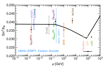
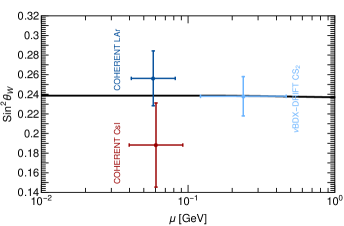
Figure 7: Left graph: Weak mixing angle RGE evolution in the $\overline{\text{MS}}$ renormalization scheme as calculated in Ref. Erler and Ramsey-Musolf (2005), along with a variety of measurements at different renormalization scales: Atomic parity violation (APV) Wood et al. (1997); Dzuba et al. (2012), MINER Agnolet et al. (2017); Cañas et al. (2018), CONNIE Aguilar-Arevalo et al. (2019); Cañas et al. (2018) (slightly offset horizontally for clarity), proton weak charge ($Q_{\text{Weak}}(P)$) from cesium transitions Androić et al. (2018), electron weak charge ($Q_{\text{Weak}}(e)$) from Møller scattering Anthony et al. (2005), parity violation in electron deep inelastic scattering (eDIS) Wang et al. (2014), neutrino-nucleus scattering (NuTeV) Zeller et al. (2002) and collider measurements (Tevatron, LEP and LHC. LEP and LHC results offset horizontally as indicated by the arrows) Tanabashi et al. (2018). Results for the DUNE near detector using elastic neutrino-electron scattering are displayed as well de Gouvea et al. (2020). The result for $\nu$BDX-DRIFT follows from the chi-square analysis in the left graph in Fig. 6 and the error bar has been reduced by a factor 2 to allow comparison with the other experiments. Right graph: Same as left graph but for fixed-target CE$\nu$NS experiments, COHERENT CsI[Na] Akimov et al. (2017); Papoulias and Kosmas (2018) and LAr Akimov et al. (2020b); Miranda et al. (2020). This result shows that measurements at $\nu$BDX-DRIFT can be more competitive that those obtained so far with COHERENT data, thus providing complementary information in the nuclear recoil channel to DUNE near detector measurements using the electron channel instead.

To put in perspective the precision that can be achieved at $\nu$BDX-DRIFT, we have plotted the RGE evolution of the weak mixing angle in the $\overline{\text{MS}}$ renormalization scheme along with the low-energy measurements of the high precision experiments we have discussed. We have as well included expectations from the DUNE near detector using elastic neutrino-electron scattering de Gouvea et al. (2020). The result is shown in Fig. 7, left graph. To allow comparison we have reduced the error bar by a factor $2$. One can see that although $\nu$BDX-DRIFT comes with a larger uncertainty than these high-precision experiments, it brings information at a renormalization scale which is not covered by any of those experiments. We note that the precise location of the scale constrained by the experiment depends on detectors parameters such as the assumed recoil threshold and the shape of the neutrino spectrum. In Fig. 7 we simply plot it at the scale corresponding to the mean recoil energy, which we find agrees within uncertainty with a more rigorous calculation accounting for the shape of the neutrino spectrum. Note that the result we obtain is expected, as it is known that reaching order $\pm 1\%$ precision in neutrino scattering experiments is challenging Kumar et al. (2013).

Note that if one focuses on experiments that fall within the same “category” (stopped-pion CE$\nu$NS-related experiments) then a more reliable comparison can be done. The right graph in Fig. 7 shows the $1\sigma$ sensitivities for COHERENT CsI[Na] and LAr along with what can be achieved at $\nu$BDX-DRIFT. We have included as well the $\mu=\langle q\rangle$ range that these experiments cover. For that we have used $q^{2}=2m_{N}E_{r}$ along with information on the minimum and maximum recoil energies these experiments have measured, or will in the case of $\nu$BDX-DRIFT: COHERENT CsI[Na], $E_{r}\subset[5,30]\,\text{keV}$ Akimov et al. (2017); COHERENT LAr, $E_{r}\subset[19,81]\,\text{keV}$ Akimov et al. (2020b); $\nu$BDX-DRIFT CS₂, $E_{r}\subset[101,2640]\,\text{keV}$. For the latter we have used $E_{\nu}^{\text{min}}=39\,$MeV and $E_{\nu}^{\text{min}}=200\,$MeV, values dictated by the neutrino spectrum low-energy tail and the coherence condition. These values result in

$$\text{CsI}: \quad q\subset[35,86]\times 10^{-3}\,\text{GeV}\ ,$$

$$\text{LAr}: \quad q\subset[38,78]\times 10^{-3}\,\text{GeV}\ ,$$

$$\text{CS}_{2}: \quad q\subset[78,397]\times 10^{-3}\,\text{GeV}\ ,$$ (14)

and $\langle q\rangle=61\times 10^{-3}\,$ GeV, $\langle q\rangle=58\times 10^{-3}\,$ GeV and $\langle q\rangle=238\times 10^{-3}\,$ GeV, respectively. One can see that among those stopped-pion CE$\nu$NS experiments $\nu$BDX-DRIFT has a better performance.

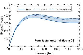
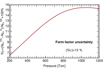
Figure 8: Left graph: CE$\nu$NS event yield as a function of pressure for carbon dioxide assuming a ten-cubic meter detector volume and 7-years data taking. The calculation has been done assuming three different form factor parametrizations: Helm form factor, symmetrized Fermi form factor and Klein-Nystrand form factor. The result shows that the smallest (largest) event yield is obtained from the Helm (Klein-Nystrand) form factor. Right graph: Percentage uncertainty as a function of pressure calculated from the minimum and maximum event yields. As pressure increases the difference increases as well as a result of increasing neutrino energy.

IV.2.2 Form factor uncertainties and measurements of neutron density distributions

Given the recoil energies involved in the $\nu$BDX-DRIFT experiment, one expects the CE$\nu$NS event yield to be rather sensitive to nuclear physics effects. Thus to assess the degree at which these effects affect CE$\nu$NS predictions, we first calculate the intrinsic uncertainties due to the form factor parametrization choice. For that aim we use—in addition to the Helm form factor parametrization Helm (1956)—the Fourier transform of the symmetrized Fermi distribution and the Klein-Nystrand form factor Sprung and Martorell (1997); Klein and Nystrand (1999).

The Helm model assumes that the proton and neutron distributions are dictated by a convolution of a uniform density of radius $R_{0}$ and a Gaussian profile characterized by the folding width $s$, responsible for the surface thickness. The Helm form factor then reads Helm (1956)

$$F_{\text{H}}(q^{2})=3\frac{j_{1}(qR_{0})}{qR_{0}}e^{-(qs)^{2}/2}\ ,$$ (15)

where $j_{1}$ is the spherical Bessel function of order one and $R_{0}$, the diffraction radius, is determined by the surface thickness and the rms radius of the corresponding distribution, namely Lewin and Smith (1996)

$$R_{0}=\sqrt{\frac{5}{3}\left(\langle r^{2}\rangle_{\text{H}}-3s^{2}\right)}\ .$$ (16)

For the surface thickness we use $0.5\,$fm Lewin and Smith (1996). The symmetrized Fermi form factor follows instead from the symmetrized Fermi function, defined through the conventional Fermi or Woods-Saxon function. The resulting form factor is given by Sprung and Martorell (1997)

$$F_{\text{SF}}(q^{2})= \frac{3}{qc}\left[\frac{\sin(qc)}{(qc)^{2}}\left(\frac{\pi qa}{\tanh(\pi qa)}-\frac{\cos(qc)}{qc}\right)\right]$$

$$\frac{\pi qa}{\sinh(\pi qa)}\frac{1}{1+(\pi a/c)^{2}}\ .$$ (17)

Here $c$ defines the half-density radius and $a$ the surface diffuseness, both related through the rms radius of the distribution

$$c=\sqrt{\frac{5}{3}\left(\langle r^{2}\rangle_{\text{SF}}-\frac{7}{5}(\pi a)^{2}\right)}\ .$$ (18)

For the calculation we fix $a=0.52\,$fm Piekarewicz et al. (2016). Results are rather insensitive to reasonable changes of this parameter Aristizabal Sierra et al. (2019b). Finally, the Klein-Nystrand form factor follows from folding a Yukawa potential of range $a_{k}$ over a hard sphere distribution with radius $R_{A}$. The form factor is then given by Klein and Nystrand (1999)

$$F_{\text{KN}}=3\frac{j_{1}(qR_{A})}{qR_{A}}\frac{1}{1+q^{2}a_{k}^{2}}\ .$$ (19)

In this case the radius $R_{A}$ and the potential range $a_{k}$ are related through the rms radius of distribution according to

$$R_{A}=\sqrt{\frac{5}{3}\left(\langle r^{2}\rangle_{\text{KN}}-6a_{k}\right)}\ ,$$ (20)

with the value for $a_{k}$ given by 0.7 fm Klein and Nystrand (1999).

With these results at hand we are now in a position to calculate the CE$\nu$NS event yield. We do so for carbon disulfide assuming the detector specifications used in our previous analyses. The result is displayed in Fig. 8 left graph, from which it can be seen that the event yield has a relative mild dependence on the nuclear form factor choice. The minimum and maximum values interpolate between the results obtained using the Helm and Klein-Nystrand form factors. It is worth noting that for reactor neutrinos, form factor effects are completely neglible while for SNS neutrinos (COHERENT) they are mild, of order $5\%$ or so Akimov et al. (2017). In this case the dependence is stronger, a result expected given the energy regime of the neutrino probe. Right graph in Fig. 8 shows the percentage uncertainty calculated according to

$$\mathcal{U}_{F}=\frac{N_{\text{ev}}^{\text{KN}}-N_{\text{ev}}^{\text{H}}}{N_{\text{ev}}^{\text{KN}}}\times 100\%\ ,$$ (21)

and covering pressures up to 1200 Torr. From this result it can be seen that at low recoil energy thresholds uncertainties are of order $6-7\%$, and raise up to order $16\%$ at high recoil energy thresholds. Calculation of the average uncertainty results in $\langle\mathcal{U}_{F}\rangle\simeq 13\%$. This means that calculation of SM CE$\nu$NS predictions as well as possible new physics effects always come along with such uncertainty. Note that our calculations in the previous Sections, based on the Helm form factor, should be understood as lower limit predictions of what should be expected.

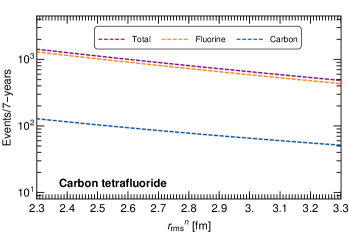
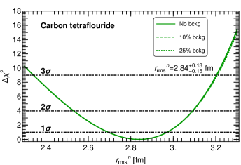
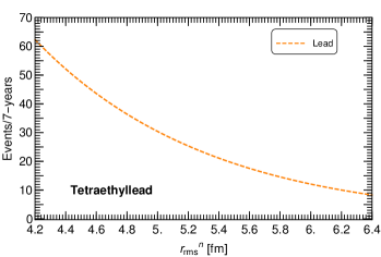
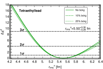
Figure 9: Top-left graph: Event distribution in terms of the neutron rms radius for $\text{C}\text{F}_{4}$. Top-right graph: Chi-square distribution for the neutron rms radii of carbon and fluorine including our three background hypotheses. For the calculation we have assumed a ten-cubic meter detector volume, 7-years data taking and 100% detector efficiency. The value for the neutron rms radius follows from the background-free case, a potential experimental scenario given the directional properties of the $\nu$BDX-DRIFT detector. We assume 100% of the detector is filled with $\text{C}\text{F}_{4}$. Bottom-left graph: Event distribution in terms of the neutron rms radius for $\text{C}_{8}\text{H}_{20}\text{Pb}$. Bottom-right graph: Chi-square distribution for the neutron rms radius of lead under the assumptions used in the carbon and fluorine case. A 2.3:1 ($\text{C}\text{S}_{2}:\text{C}_{8}\text{H}_{20}\text{Pb}$) gas ratio has been assumed. The chi-square analyses include systematics due to form factor parametrization dependences as well as neutrino flux uncertainties.

We now turn to the discussion of measurements of neutron distributions, in particular, of the rms radius of the neutron distribution. This quantity is relevant since, combined with the rms radius of the proton distribution, it defines the neutron skin thickness of a nucleus, $\Delta r_{np}(\text{nucleus})=r_{\text{rms}}^{n}-r_{\text{rms}}^{p}$. This quantity in turn is relevant in nuclear physics as well as in astrophysics. For instance, in nuclear physics it plays an important role in the nuclear energy density functional Reinhard and Nazarewicz (2010); Reinhard et al. (2013); Nazarewicz et al. (2014); Chen and Piekarewicz (2015, 2014), while in astrophysics it allows the prediction of neutron star properties such as its density and radius Horowitz and Piekarewicz (2001).

A clean direct measurement of the neutron rms radius has been done only for ${}^{208}\text{Pb}$ by the PREX experiment at the Jefferson laboratory Abrahamyan et al. (2012); Horowitz et al. (2014a). The rms radii for other nuclides have been mapped using hadronic experiments, and suffer from large uncontrolled uncertainties Horowitz et al. (2014b). In contrast to these experiments, PREX relies on parity-violating elastic electron scattering thus providing a clean determination not only of the neutron rms radius but of the neutron skin of ${}^{208}\text{Pb}$. As we have already mentioned, CE$\nu$NS experiments provide an alternative experimental avenue to determine this quantity for other nuclides.

To prove the capabilities of the $\nu$BDX-DRIFT detector we calculate sensitivities for carbon, fluorine and lead. Measurements of the rms radius of the neutron distribution for carbon and fluorine can be done using CF₄. Since carbon and fluorine have about the same amount of neutrons, in first approximation one can assume $r_{\text{rms}}^{n}|_{\text{C}}=r_{\text{rms}}^{n}|_{\text{F}}=r_{\text{rms}}^{n}$. The analysis for lead can be done using instead $\text{C}_{8}\text{H}_{20}\text{Pb}$. In this case the large mismatch between the number of neutrons for carbon and lead does not allow the approximation employed for $\text{C}\text{F}_{4}$. Experimentally, however, that measurement could be carried out by tuning pressure to the value at which the lead signal peaks (6.4 Torr) and then selecting lead events. The latter enabled by the different ranges for carbon and lead given an ionization. Following this strategy we then calculate $r_{\text{rms}}^{n}|_{\text{Pb}}$ using only the lead signal. Note that this analysis intrinsically assumes that all lead stable nuclei (²⁰⁴Pb, ²⁰⁶Pb, ²⁰⁷Pb and ²⁰⁸Pb) have the same $r_{\text{rms}}^{n}$. This of course is not the case, but it is a rather reasonble assumption given the precision at which the $r_{\text{rms}}^{n}$ can be measured at $\nu$BDX-DRIFT.

To determine sensitivities we use as toy experiment input the SM prediction assuming $r_{\text{rms}}^{n}=\langle r_{\text{rms}}^{p}\rangle$, where $\langle r_{\text{rms}}^{p}\rangle$ is calculated according to $\sum_{i}r_{\text{rms}_{i}}^{p}X_{i}$ with $r_{\text{rms}_{i}}^{p}$ the proton rms radius of $i^{\text{th}}$ stable isotope Angeli and Marinova (2013) and $X_{i}$ its natural abundance. We then perform our statistical analysis by calculating the event yield by varying $r_{\text{rms}}^{n}$ within $[2.3,3.3]\,$fm for CF₄ and $[4.2,6.4]\,$fm for $\text{C}_{8}\text{H}_{20}\text{Pb}$. Results are shown in Fig. 9. Top-left and bottom-left graphs show the variation of the event rate in terms of $r_{\text{rms}}^{n}$ for $\text{C}\text{F}_{4}$ and $\text{C}_{8}\text{H}_{20}\text{Pb}$ respectively. One can see that the signal increases with decreasing $r_{\text{rms}}^{n}$, a behavior that can be readily understood from the reduction in nuclear size implied by a smaller $r_{\text{rms}}^{n}$: As nuclear size reduces, coherence extends to larger transferred momentum.

Results of the chi-square analyses are shown in the top-right and bottom-right graphs. In each case results for our three background hypotheses are displayed. These results demonstrate that the ten-cubic meter and 7-years data taking $\nu$BDX-DRIFT will be able to set the following $1\,\sigma$ measurements:

$$\text{C and F in CF${}_{4}$}: \quad r_{\text{rms}}^{n}=2.84^{+0.13}_{-0.15}\;\text{fm}\ ,$$

$$\text{Pb in C${}_{8}$H${}_{20}$Pb}: \quad r_{\text{rms}}^{n}=5.50^{+0.30}_{-0.29}\;\text{fm}\ .$$ (22)

From these numbers one can see that the neutron rms radius for carbon and fluorine can be determined at the $3\%$ accuracy level, while for lead at about $5\%$. The difference in precision has to do with the difference in statistics. For $\text{C}\text{F}_{4}$ about 800 events are available, while for lead in $\text{C}_{8}\text{H}_{20}\text{Pb}$ only about 19 due to the constraints implied by the differentiation between lead and carbon events. Note that these measurements will not only provide information on these quantities, but can potentially be used to improve attempts to reliably extract neutron star radii, in particular those for lead.

$\boldsymbol{\nu}$BDX-DRIFT CS2    (7-years)		COHERENT CsI    (1-year)
$\epsilon_{\mu\mu}^{u}$	$[-0.013,0.011]\oplus[0.30,0.32]$	$\epsilon_{\mu\mu}^{u}$	$[-0.06,0.03]\oplus[0.37,0.44]$
$\epsilon_{e\mu}^{u}$	$[-0.064,0.064]$	$\epsilon_{e\mu}^{u}$	$[-0.13,0.13]$

Table 1: $1\sigma$ allowed ranges for neutrino NSI couplings derived from a single-parameter analysis. Results for down quark parameters are rather close to those derived for up quarks, so are not displayed. Intervals for $\epsilon_{\mu\tau}^{q}$ ($q=u,d$) are identical to those for $\epsilon_{e\mu}^{q}$. For 1-year data taking sensitivities can be degraded by up to a factor 5. Allowed $1\sigma$ limits from COHERENT CsI including spectra and timing information are taken from Ref. Giunti (2020), are shown for comparison.

IV.2.3 Sensitivities to neutrino NSI

Neutrino NSI are four-fermion contact interactions which parametrize a new vector force relative to the electroweak interaction in terms of a set of twelve flavored-dependent new parameters (in the absence of CP-violating phases). Explicitly they read Wolfenstein (1978)

$$\mathcal{L}_{\text{NSI}}=-\sqrt{2}G_{F}\sum_{q=u,d}\overline{\nu}_{a}\gamma_{\mu}(1-\gamma_{5})\nu_{b}\overline{q}\gamma^{\mu}\left(\epsilon_{ab}^{Vq}+\epsilon_{ab}^{Aq}\gamma_{5}\right)q\ ,$$ (23)

where $a,b\cdots$ are lepton flavor indices. The axial current parameters generate spin-dependent interactions and hence are poorly constrained. For that reason most NSI analyses consider only vector couplings $\epsilon_{ab}^{q}\equiv\epsilon^{Vq}_{ab}$. Limits on NSI are abundant and follow from a variety of measurements which include neutrino oscillations experiments Escrihuela et al. (2011); Gonzalez-Garcia et al. (2016), low energy scattering processes Coloma et al. (2017b) and LHC data Friedland et al. (2012); Buarque Franzosi et al. (2016). In the light of COHERENT CE$\nu$NS data they have been extensively considered as well Liao and Marfatia (2017); Papoulias and Kosmas (2018); Miranda et al. (2020); Giunti (2020); Dutta et al. (2020), and their potential experimental traces have been the subject of studies in multi-ton DM experiments Dutta et al. (2017); Aristizabal Sierra et al. (2018b); Gonzalez-Garcia et al. (2018); Aristizabal Sierra et al. (2019c).

The presence of neutrino NSI modify the CE$\nu$NS differential cross section. Being vector interactions the flavor-diagonal couplings interfere with the SM contribution, that interference can be constructive or destructive depending on the sign the coupling comes along with. In contrast, off-diagonal couplings always enhance the SM cross section. Asssuming equal rms radii for the proton and neutron distributions, the modified cross section proceeds from Eq. (1) by changing the coherent weak charge according to Barranco et al. (2005)

$$Q_{Wa}^{2} =\left[Z(g_{V}^{p}+2\epsilon_{aa}+\epsilon_{aa}^{d})+(A-Z)(g_{V}^{n}+\epsilon_{aa}+\epsilon_{aa}^{d})\right]^{2}$$

$$+\sum_{a\neq b}\left[Z(2\epsilon_{ab}^{u}+\epsilon_{ab}^{d})+(A-Z)(\epsilon_{ab}^{u}+2\epsilon_{ab}^{d})\right]^{2}\ .$$ (24)

The new parameter dependence can lead to flavor-dependent cross sections. An incoming flavor state $\nu_{a}$ can produce either the same flavor state or an orthogonal one $\nu_{b}$. The first term in Eq. (IV.2.3) accounts for $\nu_{a}\to\nu_{a}$ scattering, while the second to scattering to a flavor orthogonal state. Using the LBNF beamline, three NSI couplings—per first generation quarks—can therefore be tested: $\epsilon_{\mu\mu}^{q}$, $\epsilon_{e\mu}^{q}$ and $\epsilon_{\mu\tau}^{q}$.

Calculation of sensitivities is done assuming one parameter at a time. A procedure that is justified by the fact that is for this parameter configurations for which the best sensitivies can be derived. In all cases we vary the effective parameter in the interval $[-1.0,1.0]$. The results of the analysis are shown in Fig. 10. Left graph for $\epsilon_{\mu\mu}^{u}$ and right graph for $\epsilon_{e\mu}^{u}$ (results for down quark couplings follow closely those for up quark parameters, so are not shown). Note that due to the adopted single-parameter analysis results for $\epsilon_{\mu\tau}^{u}$ are identical to those from $\epsilon_{e\mu}^{u}$. Table 1 summarizes the $1\sigma$ sensitivities that can be achieved along with $1\sigma$ intervals derived using COHERENT CsI spectral and timing information Giunti (2020).

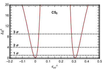
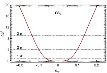
Figure 10: Left graph: Chi-Square distribution for $\epsilon_{\mu\mu}^{u}$ assuming the background-free hypothesis. Deviations due to background (10% and 25% of the signal rate) are small. For the calculation we have assumed 100% of the ten-cubic meter detector volume is filled with CS₂ and 7-years of data taking. Right graph: Same as left graph but for the off-diagonal coupling $\epsilon_{e\mu}^{u}$ (or $\epsilon_{\mu\tau}^{u}$). Results for down quark parameters are rather close to those found in this case and so are not displayed.

For the flavor-diagonal coupling we find two disconnected allowed regions, a result which is expected. The region around zero—which includes the SM solution $\epsilon_{\mu\mu}^{u}=0$—is open just because contributions from the NSI parameter generate small deviations from the SM prediction. The region of large NSI—which does not include the SM solution—is viable because the NSI and SM contributions destructively interfere, with the NSI contribution exceeding in about a factor 2 the SM terms resulting in $-|Q_{W}|\to Q_{W}$. For the off-diagonal coupling results are as well as expected. Since it contributes constructively enhancing the SM prediction, the chi-square distribution is symmetric around $\epsilon_{e\mu}^{u}=0$. Compared with results derived using COHERENT CsI spectral and timing information, one can see that in all cases sensitivities improve. For $\epsilon_{\mu\mu}^{u}$ sensitivities are better by about a factor 3 (left interval) and 1.3 (right interval). For $\epsilon_{\mu\mu}^{u}$ they improve by about a factor 2. These numbers apply as well to the other NSI parameters not displayed. All in all one can see that $\nu$BDX-DRIFT data will allow test region of NSI parameters not yet covered by COHERENT measurements.

V Conclusions

In this paper a new idea to study CE$\nu$NS with the $\nu$BDX-DRIFT detector has been considered. We have quantified sensitivities to the weak mixing angle using carbon disulfide as target material. Our findings demonstrate that a determination of this parameter at a renormalization scale within $\sim[0.1,0.4]\,$GeV can be done at the $8\%$ level, thus providing complementary information to future measurements at DUNE using the electron recoil channel. We have investigated as well sensitivities to the neutron distributions of carbon, fluorine and lead using carbon tetrafluorine and tetraethyllead as target materials. Our results show that measurements with accuracies of order $5\%$ and $10\%$, respectively, can be achieved. Finally, we have assessed sensitivities to new physics searches and for that aim we have considered effective neutrino NSI. Given the incoming neutrino flavor, at $\nu$BDX-DRIFT only muon-flavor NSI parameters can be tested. Using carbon disulfide as target material, flavor-diagonal (off-diagonal) couplings of order $10^{-3}$ ($10^{-2}$) can be proven. In the absence of a signal these numbers will translate in significant improvements of current limits.

Due to its directional and background rejection capabilities, the $\nu$BDX-DRIFT detector combined with the LBNF beamline provides a unique opportunity to study CE$\nu$NS in a neutrino energy range not yet explored. We estimated the ratio of the most important beam related neutrino-induced neutron background to the CE$\nu$NS signal to be small, about a factor 23 smaller. The detector offers a rich neutrino physics program—along with a potential agenda for light DM searches—that includes measurements of the CE$\nu$NS cross section in nuclides not used by other techonologies, measurements of the weak mixing angle in an energy regime not yet explored by any other neutrino scattering experiment, measurements of neutron distributions as well as searches for new physics in the neutrino sector.

References

- Freedman (1974) D. Z. Freedman, Phys. Rev. D9, 1389 (1974).
- Akimov et al. (2017) D. Akimov et al. (COHERENT), Science (2017), eprint 1708.01294.
- Akimov et al. (2021) D. Akimov et al. (COHERENT), Phys. Rev. Lett. 126, 012002 (2021), eprint 2003.10630.
- Wong et al. (2007) H. T. Wong et al. (TEXONO), Phys. Rev. D 75, 012001 (2007), eprint hep-ex/0605006.
- Billard et al. (2017) J. Billard et al., J. Phys. G 44, 105101 (2017), eprint 1612.09035.
- Agnolet et al. (2017) G. Agnolet et al. (MINER), Nucl. Instrum. Meth. A 853, 53 (2017), eprint 1609.02066.
- Ko et al. (2017) Y. J. Ko et al. (NEOS), Phys. Rev. Lett. 118, 121802 (2017), eprint 1610.05134.
- Aguilar-Arevalo et al. (2019) A. Aguilar-Arevalo et al. (CONNIE), Phys. Rev. D 100, 092005 (2019), eprint 1906.02200.
- Angloher et al. (2019) G. Angloher et al. (NUCLEUS), Eur. Phys. J. C 79, 1018 (2019), eprint 1905.10258.
- Akimov et al. (2020a) D. Y. Akimov et al. (RED-100), JINST 15, P02020 (2020a), eprint 1910.06190.
- Fernandez-Moroni et al. (2020) G. Fernandez-Moroni, P. A. Machado, I. Martinez-Soler, Y. F. Perez-Gonzalez, D. Rodrigues, and S. Rosauro-Alcaraz (2020), eprint 2009.10741.
- Akimov et al. (2018) D. Akimov et al. (COHERENT) (2018), eprint 1803.09183.
- Baxter et al. (2020) D. Baxter et al., JHEP 02, 123 (2020), eprint 1911.00762.
- Bellenghi et al. (2019) C. Bellenghi, D. Chiesa, L. Di Noto, M. Pallavicini, E. Previtali, and M. Vignati, Eur. Phys. J. C 79, 727 (2019), eprint 1905.10611.
- Strait et al. (2016) J. Strait et al. (DUNE) (2016), eprint 1601.05823.
- Abdullah et al. (2020) M. Abdullah, D. Aristizabal Sierra, B. Dutta, and L. E. Strigari, Phys. Rev. D 102, 015009 (2020), eprint 2003.11510.
- Snowden-Ifft et al. (2019) D. P. Snowden-Ifft, J. L. Harton, N. Ma, and F. G. Schuckman, Phys. Rev. D99, 061301 (2019), eprint 1809.06809.
- Snowden-Ifft and Gauvreau (2013) D. P. Snowden-Ifft and J. L. Gauvreau, Rev. Sci. Instrum. 84, 053304 (2013), eprint 1301.7145.
- Battat et al. (2017) J. B. R. Battat, A. C. Ezeribe, J. L. Gauvreau, J. L. Harton, R. Lafler, E. Law, E. R. Lee, D. Loomba, A. Lumnah, E. H. Miller, et al. (DRIFT), Astropart. Phys. 91, 65 (2017), eprint 1701.00171.
- Snowden-Ifft (2014) D. P. Snowden-Ifft, Rev. Sci. Instrum. 85, 013303 (2014).
- Battat et al. (2015) J. B. R. Battat, J. Brack, E. Daw, A. Dorofeev, A. C. Ezeribe, J. L. Gauvreau, M. Gold, J. L. Harton, J. M. Landers, E. Law, et al. (DRIFT), Phys. Dark Univ. 9-10, 1 (2015), eprint 1410.7821.
- Akimov et al. (2020b) D. Akimov et al. (COHERENT) (2020b), eprint 2006.12659.
- Strauss et al. (2017) R. Strauss et al., Eur. Phys. J. C77, 506 (2017), eprint 1704.04320.
- Freedman et al. (1977) D. Z. Freedman, D. N. Schramm, and D. L. Tubbs, Ann. Rev. Nucl. Part. Sci. 27, 167 (1977).
- Helm (1956) R. H. Helm, Phys. Rev. 104, 1466 (1956).
- Sprung and Martorell (1997) D. W. L. Sprung and J. Martorell, Journal of Physics A: Mathematical and General 30, 6525 (1997), URL http://stacks.iop.org/0305-4470/30/i=18/a=026.
- Klein and Nystrand (1999) S. Klein and J. Nystrand, Phys. Rev. C60, 014903 (1999), eprint hep-ph/9902259.
- Aristizabal Sierra et al. (2019a) D. Aristizabal Sierra, J. Liao, and D. Marfatia, JHEP 06, 141 (2019a), eprint 1902.07398.
- Hoferichter et al. (2020) M. Hoferichter, J. Menéndez, and A. Schwenk, Phys. Rev. D 102, 074018 (2020), eprint 2007.08529.
- Angeli and Marinova (2013) I. Angeli and K. P. Marinova, Atom. Data Nucl. Data Tabl. 99, 69 (2013).
- Burgos et al. (2007) S. Burgos et al., Astropart. Phys. 28, 409 (2007), eprint 0707.1488.
- Abi et al. (2020) B. Abi et al. (DUNE) (2020), eprint 2002.03005.
- Aristizabal Sierra et al. (2021) D. Aristizabal Sierra, B. Dutta, D. Kim, D. Loomba, D. Snowden-Ifft, and L. Strigari, Work in progress (2021).
- Snowden-Ifft (2021a) D. Snowden-Ifft, Work in progress (2021a).
- Snowden-Ifft (2021b) D. Snowden-Ifft, Work in progress (2021b).
- Kolbe and Langanke (2001) E. Kolbe and K. Langanke, Phys. Rev. C 63, 025802 (2001), eprint nucl-th/0003060.
- Formaggio and Zeller (2012) J. A. Formaggio and G. P. Zeller, Rev. Mod. Phys. 84, 1307 (2012), eprint 1305.7513.
- Agostinelli et al. (2003) S. Agostinelli et al. (GEANT4), Nucl. Instrum. Meth. A506, 250 (2003).
- Westerdale et al. (2016) S. Westerdale, E. Shields, and F. Calaprice, Astropart. Phys. 79, 10 (2016).
- Papoulias and Kosmas (2018) D. K. Papoulias and T. S. Kosmas, Phys. Rev. D97, 033003 (2018), eprint 1711.09773.
- Miranda et al. (2020) O. Miranda, D. Papoulias, G. Sanchez Garcia, O. Sanders, M. Tórtola, and J. Valle, JHEP 05, 130 (2020), eprint 2003.12050.
- Canas et al. (2016) B. Canas, E. Garces, O. Miranda, M. Tortola, and J. Valle, Phys. Lett. B 761, 450 (2016), eprint 1608.02671.
- Cañas et al. (2018) B. Cañas, E. Garcés, O. Miranda, and A. Parada, Phys. Lett. B 784, 159 (2018), eprint 1806.01310.
- de Gouvea et al. (2020) A. de Gouvea, P. A. Machado, Y. F. Perez-Gonzalez, and Z. Tabrizi, Phys. Rev. Lett. 125, 051803 (2020), eprint 1912.06658.
- Cadeddu et al. (2018) M. Cadeddu, C. Giunti, Y. F. Li, and Y. Y. Zhang, Phys. Rev. Lett. 120, 072501 (2018), eprint 1710.02730.
- Coloma et al. (2020a) P. Coloma, I. Esteban, M. C. Gonzalez-Garcia, and J. Menendez, JHEP 08, 030 (2020a), eprint 2006.08624.
- Liao and Marfatia (2017) J. Liao and D. Marfatia, Phys. Lett. B775, 54 (2017), eprint 1708.04255.
- Coloma et al. (2017a) P. Coloma, M. C. Gonzalez-Garcia, M. Maltoni, and T. Schwetz (2017a), eprint 1708.02899.
- Coloma et al. (2020b) P. Coloma, I. Esteban, M. C. Gonzalez-Garcia, and M. Maltoni, JHEP 02, 023 (2020b), [Addendum: JHEP 12, 071 (2020)], eprint 1911.09109.
- Farzan et al. (2018) Y. Farzan, M. Lindner, W. Rodejohann, and X.-J. Xu, JHEP 05, 066 (2018), eprint 1802.05171.
- Aristizabal Sierra et al. (2019b) D. Aristizabal Sierra, V. De Romeri, and N. Rojas, JHEP 09, 069 (2019b), eprint 1906.01156.
- Aristizabal Sierra et al. (2018a) D. Aristizabal Sierra, V. De Romeri, and N. Rojas, Phys. Rev. D98, 075018 (2018a), eprint 1806.07424.
- Miranda et al. (2019) O. G. Miranda, D. K. Papoulias, M. Tórtola, and J. W. F. Valle, JHEP 07, 103 (2019), eprint 1905.03750.
- Papoulias (2020) D. K. Papoulias, Phys. Rev. D 102, 113004 (2020), eprint 1907.11644.
- Dutta et al. (2019) B. Dutta, S. Liao, S. Sinha, and L. E. Strigari, Phys. Rev. Lett. 123, 061801 (2019), eprint 1903.10666.
- Kumar et al. (2013) K. Kumar, S. Mantry, W. Marciano, and P. Souder, Ann. Rev. Nucl. Part. Sci. 63, 237 (2013), eprint 1302.6263.
- Abe et al. (2000) K. Abe et al. (SLD), Phys. Rev. Lett. 84, 5945 (2000), eprint hep-ex/0004026.
- ALEPH and CDF and D0 and DELPHI and L3 and OPAL and SLD and LEP Electroweak Working Group and Tevatron Electroweak Working Group and SLD Electroweak and Heavy Flavour Groups (2010) ALEPH and CDF and D0 and DELPHI and L3 and OPAL and SLD and LEP Electroweak Working Group and Tevatron Electroweak Working Group and SLD Electroweak and Heavy Flavour Groups (2010), eprint 1012.2367.
- Wood et al. (1997) C. Wood, S. Bennett, D. Cho, B. Masterson, J. Roberts, C. Tanner, and C. E. Wieman, Science 275, 1759 (1997).
- Dzuba et al. (2012) V. Dzuba, J. Berengut, V. Flambaum, and B. Roberts, Phys. Rev. Lett. 109, 203003 (2012), eprint 1207.5864.
- Anthony et al. (2005) P. Anthony et al. (SLAC E158), Phys. Rev. Lett. 95, 081601 (2005), eprint hep-ex/0504049.
- Zeller et al. (2002) G. P. Zeller et al. (NuTeV), Phys. Rev. Lett. 88, 091802 (2002), [Erratum: Phys. Rev. Lett.90,239902(2003)], eprint hep-ex/0110059.
- Wang et al. (2014) D. Wang et al. (PVDIS), Nature 506, 67 (2014).
- Androić et al. (2018) D. Androić et al. (Qweak), Nature 557, 207 (2018), eprint 1905.08283.
- Tanabashi et al. (2018) M. Tanabashi et al. (Particle Data Group), Phys. Rev. D 98, 030001 (2018).
- Erler and Ramsey-Musolf (2005) J. Erler and M. J. Ramsey-Musolf, Phys. Rev. D 72, 073003 (2005), eprint hep-ph/0409169.
- Lewin and Smith (1996) J. D. Lewin and P. F. Smith, Astropart. Phys. 6, 87 (1996).
- Piekarewicz et al. (2016) J. Piekarewicz, A. R. Linero, P. Giuliani, and E. Chicken, Phys. Rev. C94, 034316 (2016), eprint 1604.07799.
- Reinhard and Nazarewicz (2010) P.-G. Reinhard and W. Nazarewicz, Phys. Rev. C 81, 051303 (2010), eprint 1002.4140.
- Reinhard et al. (2013) P.-G. Reinhard, J. Piekarewicz, W. Nazarewicz, B. Agrawal, N. Paar, and X. Roca-Maza, Phys. Rev. C 88, 034325 (2013), eprint 1308.1659.
- Nazarewicz et al. (2014) W. Nazarewicz, P.-G. Reinhard, W. Satula, and D. Vretenar, Eur. Phys. J. A 50, 20 (2014), eprint 1307.5782.
- Chen and Piekarewicz (2015) W.-C. Chen and J. Piekarewicz, Phys. Lett. B 748, 284 (2015), eprint 1412.7870.
- Chen and Piekarewicz (2014) W.-C. Chen and J. Piekarewicz, Phys. Rev. C 90, 044305 (2014), eprint 1408.4159.
- Horowitz and Piekarewicz (2001) C. Horowitz and J. Piekarewicz, Phys. Rev. Lett. 86, 5647 (2001), eprint astro-ph/0010227.
- Abrahamyan et al. (2012) S. Abrahamyan et al., Phys. Rev. Lett. 108, 112502 (2012), eprint 1201.2568.
- Horowitz et al. (2014a) C. Horowitz, K. Kumar, and R. Michaels, Eur. Phys. J. A 50, 48 (2014a), eprint 1307.3572.
- Horowitz et al. (2014b) C. Horowitz, E. Brown, Y. Kim, W. Lynch, R. Michaels, A. Ono, J. Piekarewicz, M. Tsang, and H. Wolter, J. Phys. G 41, 093001 (2014b), eprint 1401.5839.
- Giunti (2020) C. Giunti, Phys. Rev. D 101, 035039 (2020), eprint 1909.00466.
- Wolfenstein (1978) L. Wolfenstein, Phys. Rev. D17, 2369 (1978).
- Escrihuela et al. (2011) F. J. Escrihuela, M. Tortola, J. W. F. Valle, and O. G. Miranda, Phys. Rev. D 83, 093002 (2011), eprint 1103.1366.
- Gonzalez-Garcia et al. (2016) M. C. Gonzalez-Garcia, M. Maltoni, and T. Schwetz, Nucl. Phys. B908, 199 (2016), eprint 1512.06856.
- Coloma et al. (2017b) P. Coloma, P. B. Denton, M. C. Gonzalez-Garcia, M. Maltoni, and T. Schwetz, JHEP 04, 116 (2017b), eprint 1701.04828.
- Friedland et al. (2012) A. Friedland, M. L. Graesser, I. M. Shoemaker, and L. Vecchi, Phys. Lett. B 714, 267 (2012), eprint 1111.5331.
- Buarque Franzosi et al. (2016) D. Buarque Franzosi, M. T. Frandsen, and I. M. Shoemaker, Phys. Rev. D93, 095001 (2016), eprint 1507.07574.
- Dutta et al. (2020) B. Dutta, R. F. Lang, S. Liao, S. Sinha, L. Strigari, and A. Thompson, JHEP 20, 106 (2020), eprint 2002.03066.
- Dutta et al. (2017) B. Dutta, S. Liao, L. E. Strigari, and J. W. Walker, Phys. Lett. B773, 242 (2017), eprint 1705.00661.
- Aristizabal Sierra et al. (2018b) D. Aristizabal Sierra, N. Rojas, and M. H. G. Tytgat, JHEP 03, 197 (2018b), eprint 1712.09667.
- Gonzalez-Garcia et al. (2018) M. C. Gonzalez-Garcia, M. Maltoni, Y. F. Perez-Gonzalez, and R. Zukanovich Funchal, JHEP 07, 019 (2018), eprint 1803.03650.
- Aristizabal Sierra et al. (2019c) D. Aristizabal Sierra, B. Dutta, S. Liao, and L. E. Strigari, JHEP 12, 124 (2019c), eprint 1910.12437.
- Barranco et al. (2005) J. Barranco, O. G. Miranda, and T. I. Rashba, JHEP 12, 021 (2005), eprint hep-ph/0508299.