Analysis of Lundgren’s matched asymptotic expansion approach to the Kármán-Howarth equation using the EDQNM turbulence closure

Abstract

In this paper we investigate whether the features of the non-equilibrium cascade, which have been identified in recent studies using high-fidelity tools, can be captured in the case of the classical dissipation scaling by turbulence closures based on the statistical description of freely decaying isotropic turbulence. Numerical results obtained using the EDQNM model over a very large range of Reynolds numbers (from $Re_{\lambda}=50$ up to $Re_{\lambda}=10^{6}$) are analyzed to perform an extensive investigation of the scaling region identified as inertial range in Kolmogorov’s theory. It is observed that EDQNM results are in agreement with the results of Lundgren’s matched asymptotic expansion approach to the Kármán-Howarth equation. Both predict that the Kolmogorov inertial range equilibrium is never obtained irrespective of Reynolds number. Equilibrium is reached in the vicinity of the Taylor length $\lambda$ (which depends on viscosity) as Reynolds number tends to infinity and there is a gradual departure from equilibrium as the length scale moves away from $\lambda$, in particular towards scales larger than $\lambda$ all the way to the integral length-scale.

I Introduction

A new turbulence dissipation scaling has been discovered over the past 10 years (Vassilicos2015_arfm ; Cafiero2019_prsa and references therein) which characterises the non-equilibrium cascade in the relative near-field of various turbulent flows: grid-generated turbulence, turbulent jets, turbulent wakes and periodic turbulence (both forced and decaying). This relative near-field is in fact quite extensive in practical terms and the turbulence dissipation scaling in that relative near-field incorporates an explicit dependence on inlet/initial conditions. This scaling can be written as $\varepsilon\sim U_{0}L_{0}\mathcal{K}/L^{2}$ where $\varepsilon$ is the energy dissipation rate, $\mathcal{K}$ is the turbulent kinetic energy and $L$ is the integral length scale. On the other hand, $U_{0}$ and $L_{0}$ are a velocity scale and a length scale associated with initial/inlet conditions. Further downstream one expects no such explicit dependence, and a turbulence dissipation scaling which is the classical Taylor-Kolmogorov scaling $\varepsilon\sim\mathcal{K}^{3/2}/L$. Taylor1935_prsl ; Kolmogorov1941_dan ; Antonia2006 ; Vassilicos2015_arfm . Such a transition from one dissipation scaling to another has indeed been observed in some turbulent flows Vassilicos2015_arfm ; Goto2016_pre . However, the recent work of Goto & Vassilicos Goto2016_pre suggests that the far-field dissipation scaling is not necessarily the result of an equilibrium turbulence cascade even if it takes the exact same form as it would take in an equilibrium cascade situation.

Obligado & Vassilicos Obligado2019_epl explained why there is no equilibrium cascade at length-scales large enough to justify a Taylor-Kolmogorov dissipation scaling in the case of freely decaying homogeneous isotropic turbulence (HIT) with classical Taylor-Kolmogorov dissipation scaling. The starting point is Von Karman & Howarth Karman1938_prsA equation in the form that it takes when expressed for structure functions as in Landau & Lifschitz Landau1987 :

$$-{2\over 3}\varepsilon-{1\over 2}{\partial\over\partial t}S_{2}={1\over 6r^{4}}{\partial r^{4}S_{3}\over\partial r}-{\nu\over r^{4}}{\partial\over\partial r}(r^{4}{\partial S_{2}\over\partial r})$$ (1)

where $\varepsilon$ is the turbulence dissipation rate, $\nu$ is the kinematic viscosity of the fluid, $r$ is the distance between the pairs of points defining the second and third order longitudinal structure functions $S_{2}$ and $S_{3}$ respectively. Using Lundgren’s lundgren2002 analysis of the Kármán-Howarth equation 1 based on matched asymptotic expansions and wind tunnel data for grid-generated approximate HIT conditions, they demonstrated that spectral equilibrium can only be achieved in the vicinity of the Taylor length-scale when the Reynolds number tends to infinity. For any Reynolds number, including in the limit of infinite Reynolds number, the cascade remains out of equilibrium at any other length-scale which is not a fixed multiple of $\lambda$. The larger the length-scale compared to $\lambda$ the wider the departure from equilibrium. Without equilibrium at length-scales large enough to be independent of viscosity it is not possible to justify the Taylor-Kolmogorov dissipation scaling by a balance between the turbulence dissipation $\varepsilon$ and the large-scale interscale energy flux (or rate of energy injection into the cascade at the large scales). Goto & Vassilicos Goto2016_pre justified the far-field Taylor-Kolmogorov dissipation scaling on the basis of their concept of balanced non-equilibrium to which we return at the end of this paper.

The features of the non-equilibrium cascade have been up to now studied using high-fidelity tools such as experiments and direct numerical simulations. In this paper we investigate whether features of the non-equilibrium cascade can be captured by turbulence closures based on the statistical description of freely decaying isotropic turbulence. To this purpose, the EDQNM model Orszag1970_jfm has been identified. This tool can be used to investigate the statistical features of homogeneous turbulence and in particular the time evolution of freely decaying isotropic turbulence in a far field state. Bos2007_pof ; Lesieur2008_springer ; Meldi2013_jot ; Sagaut2018_springer . One of the main favorable features of this model is that it can be used to investigate freely decaying HIT at Reynolds numbers which are not reachable by high-fidelity tools. The present analysis provides answers to two main questions. The first one is whether the EDQNM is consistent with the absence of interscale equilibrium at all Reynolds numbers in the far field except at scales in the vicinity of the Taylor length scale. The second one is if there is agreement between EDQNM and Lundgren’s lundgren2002 matched asymptotic expansion analysis of the Karman-Howarth equation.

The paper is organized as follows. In section 2 we describe the EDQNM model we use and in section 3 we present our results and the answers to the questions we posed in this introduction. We conclude in section 4.

II The EDQNM model

The EDQNM model (Orszag1970_jfm, ; Lesieur2008_springer, ; Sagaut2018_springer, ) is a turbulence closure in spectral space. It resolves the numerical discretization of the classical Lin equation:

$$\frac{\partial E(k,t)}{\partial t}+2\nu k^{2}E(k,t)=T(k,t)+F(k,t)$$ (2)

where $F(k,t)$ is a forcing term in the spectral space to be explicitely provided. Present calculations are performed for freely decaying HIT, so $F(k,t)=0$. $T(k,t)$ is the non-linear energy transfer. This term is related to the interscale energy flux via the expression $\Pi(k,t)=\int_{k}^{+\infty}T(k,t)dk$. Integrating the Lin equation one obtains an equation where $\Pi(k,t)$ appears rather than $T(k,t)$ and which is the spectral space equivalent of the Kármán-Howarth equation 1 (see lundgren2002 and references therein). The EDQNM model is based on two fundamental assumptions applied to the evolution equation of the three-point third-order velocity correlation, which is used to calculate $T(k,t)$:

1. The quasi-normal (QN) approximation is used to express fourth-order moments by a sum of products of second-order moments. The fourth-order cumulants (i.e. deviation from a Gaussian pdf of the velocity derivatives) are represented via a linear damping term which is governed by the eddy damping rate $\eta_{E}$.

2. A Markovianization procedure is used assuming that the relaxation time of the third-order correlations is small when compared with the relaxation time of the second-order correlations.

Using these two hypotheses, a closed expression for $T(k,t)$ is obtained:

$$T(k,t)=\int_{p+q=k}\Theta_{kpq}(xy+z^{3})E(q,t)[E(p,t)pk^{2}-E(k,t)p^{3}]\frac{dpdq}{pq}$$ (3)

where $[k,p,q]$ represents the spectral system of coordinates and $xy+z^{3}$ is a geometric factor determined by the shape of the triangles respecting the condition $p+q=k$ in the spectral space. The term $\Theta_{kpq}^{-1}=\eta_{E}(k,t)+\eta_{E}(p,t)+\eta_{E}(q,t)$ is a spectral time scale which is inversely proportional to the eddy damping rate $\eta_{E}$. This term is usually derived by the following model relation Pouquet1975_jfm :

$$\eta_{E}(k,t)=A\,\sqrt{\int_{0}^{k}\,p^{2}E(p,t)\,dp}+\nu k^{2}.$$ (4)

The free coefficient $A\in[0.3,\,0.5]$ is usually set to optimize the value for the constant $C_{K}$ governing $E$ in the scaling region i.e. $E(k,t)=C_{K}\varepsilon^{2/3}k^{-5/3}$ Andre1977_jfm . A different model for the determination of the eddy damping term is the EDQNM-LMFA proposed by Bos & Bertoglio Bos2006_pof . In this model, the eddy damping rate $\eta_{E}$ is calculated using a model equation for the velocity derivative cross-correlation $\mathcal{F}_{CC}$, so that $\eta_{E}(k,t)=E(k,t)/\mathcal{F}_{CC}(k,t)+\nu k^{2}$.

The turbulent kinetic energy $\mathcal{K}(t)$, the energy dissipation rate $\varepsilon(t)$ and all the other physical quantities are derived via manipulation or integration of $E(k,t)$ and $T(k,t)$. The calculations are performed using an adaptive spectral mesh strategy (Meldi2014_jcp, ) which preserves both the large-scale and the small-scale resolution. This operation is performed by updating the mesh elements so that the conditions $k_{L}(t)/k_{min}(t)=s_{L}=const$ and $k_{\eta}(t)/k_{max}(t)=s_{\eta}=const$ are verified. Here, $k_{L}(t)=L^{-1}(t)$ is the wave number associated with the integral length scale $L$, $k_{\eta}(t)=\eta^{-1}(t)$ is the wave number associated with the Kolmogorov scale $\eta$, $k_{max}$ is the largest resolved mode and $k_{min}$ is the smallest resolved mode. This strategy allows for the complete control of confinement effects. For every calculation $s_{\eta}=10^{-1}$ is imposed, which implies that the smallest resolved scale has a size of $\approx 0.1\eta$. More details about the value of the constant $s_{L}$ are provided below.

A database of EDQNM calculations has been established in order to quantify the sensitivity of the physical quantities investigated to variations in the set up of the problem as detailed in the following list.

• Initial conditions. Different proposals have been employed to initialize the energy spectrum at time $t=0$ of the free decay simulations. The first one is inspired from the functional form found in Pope Pope2000_cambridge and Meyers & Meneveau Meyers2008_pof :

  $$E_{I}(k,t=0)=C_{K}\,{\varepsilon}^{2/3}k^{-5/3}f_{L}(kL)f_{\eta}(k\eta)$$ (5)

  with

  $$f_{L}(kL)=\left(\frac{kL}{[(kL)^{1.5}+c_{L}]^{1/1.5}}\right)^{5/3+\sigma}\>,\hskip 1.42271ptf_{\eta}(k\eta)=\exp(-\beta([(k\eta)^{4}+c_{\eta}^{4}]^{1/4}-c_{\eta}))$$ (6)

  where $C_{K}\approx 1.6$ is the Kolmogorov constant. The dimensionless coefficients in equations 5 - 6 have been set to $c_{\eta}=0.4$, $\beta=5.3$; $c_{L}$ has been chosen such as to obtain $L(0)=1$. The parameter $\sigma$, which controls the shape of the energy spectrum at the large scales, is discussed separately analyzed in the next bullet point. A second functional form employed to initialise the energy spectrum at $t=0$ is the classical exponential relation

  $$E(k,t=0)=k^{\sigma}\exp((-\sigma/2)k^{2})$$ (7)

  which is controled by the parameter $\sigma$ only.

• Large scale parameter $\sigma$. This parameter is strictly concerned with the initialization procedure described above, but the effects of $\sigma$ on HIT decay do not disappear if sufficient resolution is provided at the large scales Meldi2012_jfm ; Meldi2017_jfm . The values chosen for this parameter are $\sigma=2,4$ which correspond to the well known cases of Saffman turbulence and Loitsiansky turbulence, respectively.

• EDQNM model. Runs have been perfomed using both the classical version of EDQNM and the EDQNM-LMFA model.

• Resolution at the large scales. The last aspect of the sensitivity analysis deals with confinement i.e. lack of resolution at the large scales. Most of the simulations in the database are run using $s_{L}=500$, which ensures that confinement effects are completely excluded. One simulation is instead run for $s_{L}=10$, in order to investigate the effects of saturation over the physical quantities investigated.

Simulation Nr.	Functional form ($t=0$)	$\sigma$	EDQNM model	$k_{L}(t)/k_{min}(t)$
$1$	Pope (eq. 5 - 6)	$2$	LMFA	$500$
$2$	Pope	$2$	LMFA	$10$
$3$	Pope	$4$	LMFA	$500$
$4$	Pope	$4$	classical	$500$
$5$	exponential (eq. 7)	$2$	classical	$500$
$6$	exponential	$4$	classical	$500$
$7$	exponential	$4$	LMFA	$500$

Table 1: Database of EDQNM calculations used in the present analysis.

A summary of the features of the calculations included in the database is reported in table 1. Every calculation of the database is performed using an initial Reynolds number of $Re_{\lambda}(t=0)=10^{6}$. A transient regime is initially observed, which is governed by the features of the functional form prescribed for $t=0$. During this transient, the Reynolds number increases up to $Re_{\lambda}\approx 2\times 10^{6}$ at $t\approx t_{0}$, where $t_{0}=\mathcal{K}(t=0)/\varepsilon(t=0)$ is the initial turnover time. After this first phase, the statistics progressively lose memory of those initial condition prescribed in the scaling range and in the small scale region. A classical power law decay is then observed (Comte-Bellot1966_jfm, ; Meldi2012_jfm, ), which is governed by the parameter $\sigma$ prescribed in the functional form of $E$. This parameter controls the slope of the energy spectrum at the very large scales. Data in the form of $E(k,t)$ are sampled in the range $t/t_{0}\in[10^{3},\,10^{C}]$, which corresponds to a free decay from $Re_{\lambda}(t/t_{0}\approx 10^{3})=10^{6}$ to $Re_{\lambda}(t/t_{0}\approx 10^{C})=50,\,C\in[25,45]$. The time range chosen for sampling varies with initial conditions and with value of $\sigma$ in particular.

Results are now discussed for simulation 1 of the database. For this simulation the effects of the functional form prescribed at $t=0$, which are measured via the rate of convergence towards the expected power-law decay exponent, can be estimated to be $\approx 5\%$ for $Re_{\lambda}=10^{6}$ and $<0.1\%$ for $Re_{\lambda}=10^{5}$. The energy spectrum $E$, the compensated energy spectrum $E/(\varepsilon^{2/3}k^{-5/3})$, the derivative of the non-linear energy transfer $T$ and the interscale energy flux $\Pi$ are shown for $Re_{\lambda}=10^{6},\,10^{5},\,10^{4},\,10^{3},\,10^{2}$ in figure 1. The EDQNM results we obtain comply with previous EDQNM results Bos2007_pof ; Meldi2013_jot and, plotted as in this figure and without further analysis, may appear to support the picture drawn by the $K41$ theory Kolmogorov41a ; Kolmogorov41b for $Re_{\lambda}\to+\infty$. The compensated energy spectrum as well as the non-linear energy transfer collapse remarkably well in the small scale region when plotted against $k\eta$. In addition, one can see the emergence of a scaling range for sufficiently high $Re_{\lambda}$ (larger than $10^{4}$ according to present data). This range, which can be described by the relation $E(k)=C_{K}\varepsilon^{2/3}k^{-5/3}\approx 1.6\varepsilon^{2/3}k^{-5/3}$ to a close approximation, appears to be characterized by a close-to-zero derivative of the non linear energy transfer and by $\Pi/\varepsilon\approx 1$, which one may infer from figure 1(d).

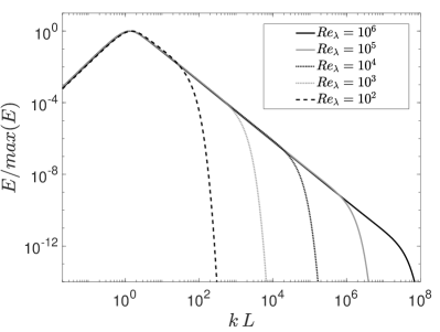
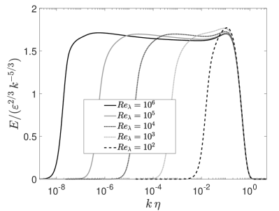
(a)	(b)
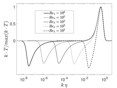
(c)	(d)

Figure 1: Energy spectrum and non-linear energy transfer calculated via EDQNM. (a) Normalized energy spectrum $E/max(E)$. (b) Compensated energy spectrum $E/(k^{-5/3}\varepsilon^{2/3}$). (c) Normalized derivative in Fourier space of the non-linear energy transfer budget term, $kT/max(kT$). (d) Normalized inter scale energy flux $\Pi/\varepsilon$.

The EDQNM predictions for $E$ and $T$ are used to obtain expressions for second-order and third-order structure functions. These quantities can be calculated exactly via the following integral / differential relations (Tchoufag2012_pof, ; Bos2012_pof, ):

$$S_{2}(r,t) = \int_{0}^{+\infty}4\,E(k,t)\,\left[\frac{1}{3}-\frac{sin(kr)-(kr)cos(kr)}{(kr)^{3}}\right]\,dk$$ (8)

$$S_{3}(r,t) = \int_{0}^{+\infty}12\,T(k,t)\,\frac{3(sin(kr)-(kr)cos(kr))-(kr)^{2}sin(kr)}{(kr)^{5}}\,dk$$ (9)

$$f(r,t) = -\frac{1}{\varepsilon}\frac{\partial S_{2}(r,t)}{\partial t}$$ (10)

$$F(r,t) = -\frac{3}{\varepsilon r^{5}}\int_{0}^{r}{r^{\prime}}^{4}\frac{\partial S_{2}}{\partial t}\,dr^{\prime}$$ (11)

where $S_{2}$ is the second-order moment of the longitudinal velocity increment, $S_{3}$ is the third-order moment and $f$ and $F$ are non-stationarity functions Obligado2019_epl . These non-stationarity functions measure the departure from equilibrium scale by scale and appear naturally from the form of the Kármán-Howarth equation (1) given by Landau & Lifschitz Landau1987 (see also Danaila99 ; lundgren2002 ). The $-4/5$ law $S_{3}\approx-{4\over 5}\varepsilon r$ might be derived from this equation in a range of scales $r$ where $F\approx 0$ (implying equilibrium) and viscous diffusion is negligible. The function $F$ is obtained by a normalised integration of the non-stationarity function $f$ which is directly interpretable in terms of equilibrium as it is small at a given scale $r$ and a given time $t$ if $\frac{\partial S_{2}(r,t)}{\partial t}$ is small compared to ${\varepsilon}$. The question which was raised by Obligado & Vassilicos Obligado2019_epl concerns the range of scales where one might safely assume $F\approx 0$ and this is part of the questions which we now address in terms of EDQNM.

III Results

Results presented in this section are again taken from simulation 1 of the database. Data are first compared with experimental results in Obligado & Vassilicos Obligado2019_epl . The non-stationarity function $f$ is shown in figure 2 for $Re_{\lambda}=50,380$. The comparison shows that there is reasonable agreement for low to moderate Reynolds numbers, in particular for small values of $r$. The EDQNM prediction appears to increase slightly faster towards the asymptotic value $f=4/3$ for large $r$ values. However, the difference between EDQNM results and grid turbulence data is small, not larger than $\approx 10\%$ in magnitude on this non-stationarity/non-equilibrium function. This validation supports the view that one might reasonably expect EDQNM data for much higher Reynolds numbers (up to $Re_{\lambda}=10^{6}$) to provide an estimation of the behavior of the physical quantities investigated, such as $f$ and $F$.

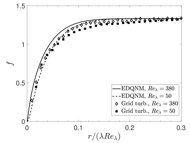
Figure 2: Non-stationarity function $f$. EDQNM results are compared with experimental grid turbulence results.

The EDQNM predictions for $f$ and $F$ are shown in figure 3. In the left column, $f$ is plotted against $r/L$, $r/\lambda$ and $r/\eta$ from top to bottom. Two asymptotic behaviors are observed for small and large values of $r$. (i) One can see that $f$ converges towards a constant value of $f=4/3$ for $r>2L$ in agreement with basic theory (see Obligado2019_epl ). The way the EDQNM profiles reach the asymptote is the same in terms of $r/L$ as the curves collapse significantly well even before reaching the asymptotic value in 3(a). (ii) On the other hand, $f\propto r^{2}$ at the small scales which also agrees with basic theory Taylor1935_prsl . This range appears to be fully established for $r\leq 5\eta$ approximately (see figure 3(e)). However, the curves do not collapse for any value of $r$ when plotted against $r/\eta$. Self-preservation at the small scales is instead obtained when using a $r/\lambda$ horizontal axis, as shown in figure 3(c). This result confirms that the EDQNM prediction comply very well with power-law turbulence decay and the theoretical result $f\approx(r/\lambda)^{2}(-\frac{\mathcal{K}}{\varepsilon^{2}}\frac{d\varepsilon}{dt})$ in the small scale region Taylor1935_prsl ; Obligado2019_epl . The power-law decay implies that $(-\frac{\mathcal{K}}{\varepsilon^{2}}\frac{d\varepsilon}{dt})$ is independent of time and that the entire time-dependence and/or Reynolds number dependence of $f$ at scales $r\leq 5\eta$ is therefore captured by $f\approx(r/\lambda)^{2}$, hence the collapse in figure 3(c) which EDQNM is able to reproduce.

If the Reynolds number is sufficiently high, a scaling range where $f\propto r^{2/3}$ emerges between the large scale region and the small scale region. This range can be qualitatively observed for $Re_{\lambda}\geq 10^{3}$. In addition, the scaling predicted by EDQNM in this range complies very well with the formula $f=-1.5(\frac{d\varepsilon}{dt}/\varepsilon)(r/\sqrt{\varepsilon})^{2/3}$ which follows from $S_{2}\approx{9\over 4}(\varepsilon r)^{2/3}$.

The analysis of the non-stationarity function $F$, which is reported on the right column of figure 3, allows to draw almost identical conclusions. The only observable difference is the value of the asymptotic limit in the large scale region, which is $F=4/5$ in agreement with basic theory Obligado2019_epl .

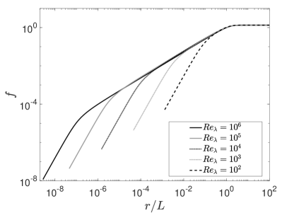
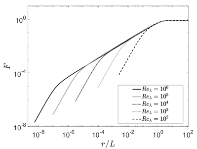
(a)	(b)
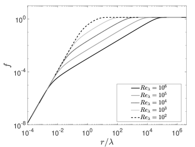
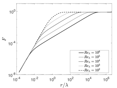
(c)	(d)
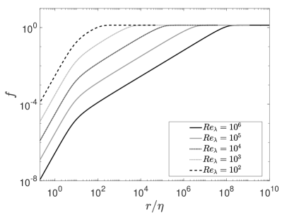
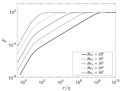
(e)	(f)

Figure 3: Non-stationarity functions (left column) $f$ and (right column) $F$ represented against (first row) $r/L$, (second row) $r/\lambda$ and (third row) $r/\eta$.

Results are further analyzed to obtain more accurate information about the features of the ranges approximately identified. In figure 4 the exponent $n_{f}(r)=d\,log(f)/d\,log(r)$ is reported: it is calculated via polynomial fitting from the EDQNM results. This parameter indicates that a scaling range for which $f\propto r^{2/3}$ is observed for at least one decade only for $Re_{\lambda}\geq 10^{4}$. In addition, if one excludes the curve for the lowest Reynolds number $Re_{\lambda}=10^{2}$, the inflection point for $n_{f}$ is at $r/\lambda\approx 5$ for all Reynolds numbers.

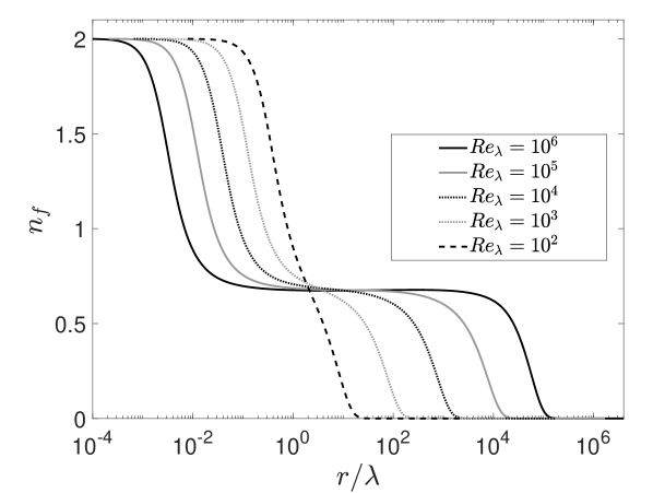
Figure 4: Exponent for a power-law $r$-dependence of the non-stationarity function $f$. The function is represented as $f\propto r^{n_{f}(r)}$, where $n_{f}(r)$ is the local power law exponent. It is determined via local logarithmic polynomial fitting.

As already observed, $f$ profiles do not collapse when plotted against $r/\eta$ and they exhibit self-preservation in the small scale region when plotted against $r/\lambda$. However, given that $\lambda/\eta\propto Re_{\lambda}^{1/2}$, it follows from $f\approx(r/\lambda)^{2}(-\frac{\mathcal{K}}{\varepsilon^{2}}\frac{d\varepsilon}{dt})$ that $fRe_{\lambda}\approx(r/\eta)^{2}(-\frac{\mathcal{K}}{\varepsilon^{2}}\frac{d\varepsilon}{dt})$ where $(-\frac{\mathcal{K}}{\varepsilon^{2}}\frac{d\varepsilon}{dt})$ is independent of time and Reynolds number for a power-law turbulence decay. The EDQNM prediction complies with this formula, which is shown in figure 5. The function $fRe_{\lambda}$ exhibits partial self-preservation in the small scale region but also in the intermediate scaling range when plotted against $r/\eta$.

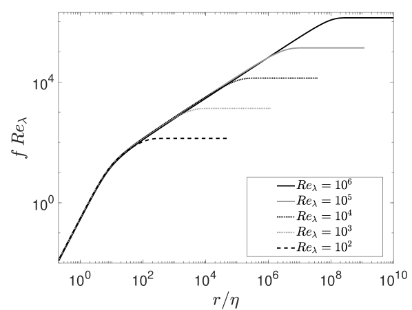
Figure 5: Non-stationarity function $f$ times the Reynolds number $Re_{\lambda}$.

We now investigate detailed EDQNM predictions for the interscale energy flux $\Pi$ and the third order structure function $S_{3}$ which are central quantities for characterising the equilibrium or non-equilibrium of the turbulence cascade. The function $1-\Pi/\varepsilon$ is plotted in logarithmic scale in figure 6(a). According to Kolmogorov equilibrium, the value of this function should be zero in some inertial range if the Reynolds number is large enough. However, the equilibrium $\Pi/\varepsilon=1$ is never observed over an inertial (i.e. viscosity-independent) range for any Reynolds number. The value of $r$ where $\Pi/\varepsilon$ is closest to 1 turns out to be $r=0.42\lambda$ for every $Re_{\lambda}$ in the range investigated. Indeed, the minimum for $1-\Pi/\varepsilon$ is observed for $r=0.42\lambda$ irrespective of Reynolds number in figure 7(a). As $Re_{\lambda}$ increases towards infinity, $1-\Pi/\varepsilon$ tends to $0$ only for values of $r$ which remain a fixed factor or multiple of $\lambda$ as $Re_{\lambda}$ varies. In other words the tendency towards equilibrium is only present in the vicinity of the Taylor scale $\lambda$ in perfect agreement with the prediction of Lundgren lundgren2002 and Obligado & Vassilicos Obligado2019_epl . As the Taylor scale depends on viscosity we cannot say that the tendency towards equilibrium happens in some inertial range. As figure 6(a) suggests, in a range of scales which are independent of viscosity the degree of non-equilibrium persists with increasing Reynolds number and the closer the length-scale $r$ is to $L$ the further the turbulence is from equilibrium. Results in figure 6(a) indicate that this departure from equilibrium scales as $(r/\lambda)^{2/3}$ for $r>\lambda$ and as $r/\lambda$ for $r<\lambda$. These formulae can be used to determine the span of an empirical range respecting the condition $\Pi/\varepsilon\approx 1$, down to a prescribed tollerance. In fact, if one fixes a level of tollerance $L_{T}$ tracing a horizontal line in figure 6(a) (let’s say for example $L_{T}=10^{-2}$, which corresponds to an error of $1\%$), an approximated triangle in the spectral space can be drawn intersecting this line with the curve for a selected $Re_{\lambda}$. Using the scalings introduced two sentences above this one, and considering that the vertical position of the lower vertex of the triangle can be approximated by the value $min(1-\Pi/\varepsilon)$, one can determine the extension of this empirical range $\Delta_{er}$:

$$\Delta_{er}=10^{\sigma_{er}}\,,\qquad\sigma_{er}=\left(\log_{10}(P_{r})-\log_{10}(min(1-\Pi/\varepsilon))\right)\left(1+\frac{3}{2}\right)$$ (12)

The coefficient (1+3/2) on the right is obtained from the observation of slopes $r/\lambda$ for $r<\lambda$ and $(r/\lambda)^{2/3}$ for $r>\lambda$ in figure 6(a). The span of this range increases with $Re_{\lambda}$ but it also significantly changes with the degree of tollerance imposed for the relation $\Pi/\varepsilon\approx 1$. For high $Re_{\lambda}$ and relatively low tollerance, one can obtain a significantly large range which will not be exactly centered around $\lambda$, as the function $1-\Pi/\varepsilon$ exhibits different evolutions moving from $\lambda$ towards the small scales and the large scales respectively. Such a coarse analysis may erroneously lead one to think that the condition $\Pi/\varepsilon\approx 1$ holds in some bit of an inertial range, but the fact remains that $\Pi/\varepsilon$ approaches $1$ as $Re_{\lambda}\to\infty$ only for scales $r$ around $\lambda$, i.e. in a range of scales which is not inertial.

In conclusion, the EDQNM model agrees with the matched asymptotic expansion analysis of the Kármán-Howarth equation of Lundgren lundgren2002 (confirmed by the wind tunnel data analysis of Obligado & Vassilicos Obligado2019_epl ) which predicts that there is no inertial range with an approximate equilibrium between $\Pi$ and $\varepsilon$ and that, instead, there is a systematic departure from equilibrium as scales $r$ are considered further and further away from $\lambda$. For any fixed $r/L$ value, however small, $\Pi/\varepsilon$ does not tend to 1 as $Re_{\lambda}\to\infty$, even if $r/L$ is so very small that $\Pi/\varepsilon$ is close to 1.

Similar conclusions can be drawn for $S_{3}$, which is shown in figure 6(b). Here the Kolmogorov equilibrium value $S_{3}/(\varepsilon r)=-4/5$ for HIT is never reached, except asymptotically as $Re_{\lambda}\to+\infty$ at a value of $r/\lambda$ which remains fixed as $Re_{\lambda}$ grows. In fact, Lundgren’s (2002) matched asymptotic expansion analysis of the Kármán-Howarth equation predicts that the minimum value of $4/5+S_{3}/(\varepsilon r)$ is reached at a value of $r$ which is a fixed multiple of $\lambda$ and that $4/5-max(-S_{3}/(\varepsilon r))\propto Re_{\lambda}^{-2/3}$ (see Obligado & Vassilicos 2019). Our EDQNM results are in full agreement with these predictions and return a value $r=1.12\lambda$ (see figure 7(b)) for the scale $r$ where $4/5+S_{3}/(\varepsilon r)$ is minimal and a decay towards 0 of this minimal value which is indeed proportional to $Re_{\lambda}^{-2/3}$ as $Re_{\lambda}$ increases (see figure 7(a)). More precisely, EDQNM results suggest that the minimum can be well approximated by the relation $min(1-\Pi/\varepsilon)\approx 10Re_{\lambda}^{-2/3}$.

EDQNM results for the function $1-max(\Pi/\varepsilon)$ are also shown in figure 7(a) in the range $Re_{\lambda}\in[10^{2},\,10^{5}]$. Reflecting the behaviour of $S_{3}$, $1-max(\Pi/\varepsilon)\propto Re_{\lambda}^{-2/3}$ as $Re_{\lambda}\to+\infty$ and the value of $r$ where $1-(\Pi/\varepsilon)$ takes its minimum value also scales with $\lambda$: figure 7(b) shows that this value of $r$ is $r=0.42\lambda$ for every $Re_{\lambda}$ in the range investigated.

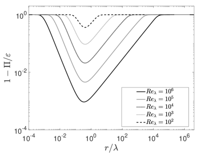
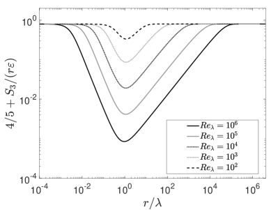
(a)	(b)

Figure 6: (a) $1-\Pi/\varepsilon$ and (b) $4/5+S_{3}/(\varepsilon r)$ represented in log-log scale.

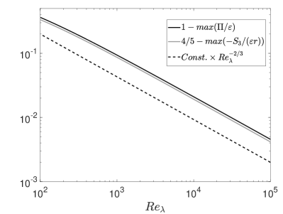
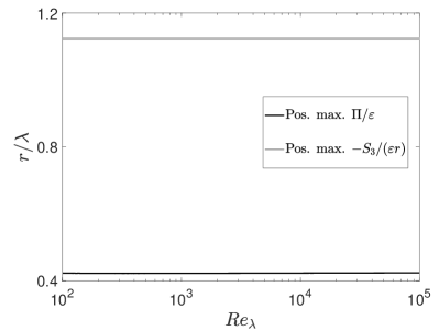
(a)	(b)

Figure 7: (a) Calculated values (for each $E$ and $T$ sampled in $Re_{\lambda}\in[10^{2},10^{5}]$) of $1-max(\Pi/\varepsilon)$ and $4/5-max(-S_{3}/(\varepsilon r))$. (b) Value of $r/\lambda$ where minima are observed.

IV Sensitivity analysis

The sensitivity of the results shown in figure 7 is now analyzed by comparing results from different simulations of our database in order to quantify the effects of the variations in the parametric description.

More specifically, the sensitivity on the parameters characterising the large scale features is investigated for $min(1-\Pi/\varepsilon)$ and for the value of $r/\lambda$ where minima are observed. This sensitivity analysis is based on results from the simulations $1$ to $7$ in our database (see table 1 for more information). The large-scale features encompass the actual parameters governing the large scales, such as $\sigma$, but also the two EDQNM models and the functional forms prescribed for $E(k,t=0)$. The results, which are shown in figure 8, show that variations in $\sigma$, in the prescribed form for $E(k,t=0)$ and in the model for the eddy-damping term in EDQNM do not significantly affect the results. However, some differences may be observed for simulation 2 at $Re_{\lambda}<400$. For this simulation, confinement effects at the large scales are more important than in the other calculations in the database. As $Re_{\lambda}$ decreases, the reduced scale separation allows the confinement effects to affect $min(1-\Pi/\varepsilon)$ and the value of $r/\lambda$ where this minimum is observed.

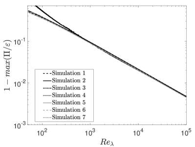
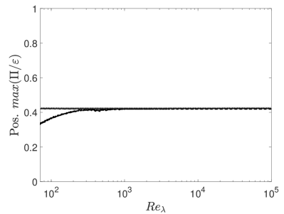
(a)	(b)

Figure 8: Sensitivity of (a) calculated values of $1-max(\Pi/\varepsilon)$ and (b) value of $r/\lambda$ where minima are observed, to the large scale features imposed in the EDQNM calculations.

V Conclusions

It is perhaps remarkable how well EDQNM of freely decaying HIT agrees with the results of Lundgren’s matched asymptotic expansion approach lundgren2002 to the Kármán-Howarth equation. Both predict that a Kolmogorov inertial range equilibrium is not obtained. Equilibrium is only achieved in the vicinity of the Taylor length in the limit where the Reynolds number tends to infinity and the Taylor length is not in the inertial range given its explicit dependence on viscosity. As the length-scale $r$ moves away from $\lambda$ and towards the integral scale $L$, the turbulence moves progressively further and further away from Kolmogorov equilibrium. The inertial range is in fact characterised by a gradually increasing departure from equilibrium as $r$ increases from $\lambda$ to $L$, not by uniform near-equilibrium over much or even a significant part of this range, however large the Reynolds number may be. At a length-scale $r$ taken to be a fixed small fraction (however small) of the integral scale, the ratio of the interscale energy flux to the turbulence dissipation does not tend to 1 a the Reynolds number tends to infinity.

Similar considerations can be extended to the case where $r$ decreases from $\lambda$ to $\eta$ except that there is no inertial range at these very small length-scales. However, this last range is significantly shorter and it can be clearly observed only for very high $Re_{\lambda}$.

This raises the question of justifying the presence of the Taylor-Kolmogorov scaling of the turbulence dissipation even though there is no equilibrium in the inertial range, particularly at the larger-scale end of it. Goto & Vassilicos Goto2016_pre introduced the concept of balanced non-equilibrium for such a justification. They considered the Lin equation integrated over wavenumbers from $k$ to infinity and defined balanced non-equilibrium to mean that the 3 terms in this integrated Lin equation vary together in time for wavenumbers $k\sim 1/L$. Balanced non-equilibrium therefore means that

$$\frac{\partial}{\partial t}\int_{1/L}^{+\infty}E(k,t)dk\sim 2\nu\int_{1/L}^{+\infty}k^{2}E(k,t)dk\sim\Pi(1/L,t)$$ (13)

which leads to the Taylor-Kolmogorov dissipation scaling given that $2\nu\int_{1/L}^{+\infty}k^{2}E(k,t)dk\approx\varepsilon$ and that $\Pi(1/L,t)$ can be considered to be independent of inlet/initial conditions and viscosity. The validity of balanced non-equilibrium was demonstrated in the context of EDQNM by Meldi & Sagaut Meldi2013_jot and therefore explains the fact that EDQNM returns the Taylor-Kolmogorov scaling for the turbulence dissipation as reported in previous publications Bos2007_pof ; Meldi2013_jot ; Sagaut2018_springer . Future potential investigations could employ more sophisticated tools able to take into account anisotropy of the flow, such as specific versions of the EDQNM model reported in the literature Mons2014_pof ; Mons2015_jfm ; Briard2016_jfm .

References

- [1] J.C. Vassilicos. Dissipation in turbulent flows. Annual Review of Fluid Mechanics, 47:95–114, 2015.
- [2] G. Cafiero and J. C. Vassilicos. Non-equilibrium turbulence scalings and self-similarity in turbulent planar jets. Proceedings of the Royal Society A, 475 (2225):20190038, 2019.
- [3] G. I. Taylor. Statistical Theory of Turbulence. Proceedings of the Royal Society of London A, 151:421–444, 1935.
- [4] A. N. Kolmogorov. On the degeneration of isotropic turbulence in an incompressible viscous fluid. Doklady Akademii nauk SSSR, 31(6):538 – 541, 1941.
- [5] R.A. Antonia and P. Burattini. Approach to the 4/5 law in homogeneous isotropic turbulence. J. Fluid Mech., 550:175–184, 2006.
- [6] S. Goto and J. C. Vassilicos. Unsteady turbulence cascades. Physical Review E, 94:053108, 2016.
- [7] M. Obligado and J. C. Vassilicos. The non-equilibrium part of the inertial range in decaying homogeneous turbulence. Europhysics Letters, 127:64004, 2019.
- [8] T. Von Karman and L. Howarth. On the statistical theory of isotropic turbulence. Proceedings of the Royal Society A, 164:192–215, 1938.
- [9] L. D. Landau and E. M. Lifshitz. Fluid mechanics: Vol 6 of course of theoretical physics, Second Edition. Pergamon Press, 1987.
- [10] Thomas S Lundgren. Kolmogorov two-thirds law by matched asymptotic expansion. Phys. Fluids, 14(2):638–642, 2002.
- [11] S. A. Orszag. Analytical theories of turbulence. J. Fluid Mech., 41:363 – 386, 1970.
- [12] W. J. T. Bos, L. Shao, and J. P. Bertoglio. Spectral imbalance and the normalized dissipation rate of turbulence. Phys. Fluids, 19(4):045101, 2007.
- [13] M. Lesieur. Turbulence in Fluids (4th edition). Springer, 2008.
- [14] M. Meldi and P. Sagaut. Further insights into self-similarity and self-preservation in freely decaying isotropic turbulence. Journal of Turbulence, 14:24–53, 2013.
- [15] P. Sagaut and C. Cambon. Homogenous Turbulence Dynamics. Springer Verlag, 2018.
- [16] A. Pouquet, M. Lesieur, J.-C. André, and C. Basdevant. Evolution of high reynolds number two-dimensional turbulence. J. Fluid Mech., 75:305–319, 1975.
- [17] J.-C. André and M. Lesieur. Influence of helicity on the evolution of isotropic turbulence at high reynolds number. J. Fluid Mech., 81:187–207, 1977.
- [18] W. J. T. Bos and J.-P. Bertoglio. A single-time two-point closure based on fluid particle displacements. Phys. Fluids, 18:031706, 2006.
- [19] M. Meldi and P. Sagaut. An adaptive numerical method for solving EDQNM equations for the analysis of long-time decay of isotropic turbulence. Journal of Computational Physics, 262:72–85, 2014.
- [20] S. B. Pope. Turbulent Flows. Cambridge University Press, 2000.
- [21] J. Meyers and C. Meneveau. A functional form for the energy spectrum parametrizing bottleneck and intermittency effects. Phys. Fluids, 20(6):065109, 2008.
- [22] M. Meldi and P. Sagaut. On non-self-similar regimes in homogeneous isotropic turbulence decay. J. Fluid Mech., 711:364–393, 2012.
- [23] M. Meldi and P. Sagaut. Turbulence in a box: Quantification of large-scale resolution effects in isotropic turbulence free decay. J. Fluid Mech., 818:697–715, 2017.
- [24] G. Comte-Bellot and S. Corrsin. The use of a contraction to improve the isotropy of grid-generated turbulence. J. Fluid Mech., 25:657 – 682, 1966.
- [25] A. N. Kolmogorov. The local structure of turbulence in incompressible viscous fluid for very large Reynolds number. Dokl. Akad. Nauk SSSR, 30 (see also Proc. R. Soc. Lond. A (1991), 434, 9-13), 1941a.
- [26] A. N. Kolmogorov. Dissipation of energy in the locally isotropic turbulence. Dokl. Akad. Nauk SSSR, 32 (see also Proc. R. Soc. Lond. A (1991), 434, 15-17), 1941b.
- [27] J. Tchoufag, P. Sagaut, and C. Cambon. Spectral approach to finite Reynolds number effects on Kolmogorov’s 4/5 law in isotropic turbulence. Phys. Fluids, 24(1):015107, 2012.
- [28] W. J. T. Bos, L. Chevillard, J. F. Scott, and R. Rubinstein. Reynolds number effect on the velocity increment skewness in isotropic turbulence. Phys. Fluids, 24:015108, 2012.
- [29] L. Danaila, F. Anselmet, T. Zhou, and R. A. Antonia. A generalization of Yaglom’s equation which accounts for the large-scale forcing in heated decaying turbulence. J. Fluid Mech., 391:359–372, 1999.
- [30] V. Mons, M. Meldi, and P. Sagaut. Numerical investigation on the partial return to isotropy of freely decaying homogeneous axisymmetric turbulence. Phys. Fluids, 26:025110, 2014.
- [31] V. Mons, C. Cambon, and P. Sagaut. A spectral model for homogeneous shear-driven anisotropic turbulence in terms of spherically averaged descriptors. J. Fluid Mech., 788:147–182, 2015.
- [32] A. Briard, T. Gomez, and C. Cambon. Spectral modelling for passive scalar dynamics in homogeneous anisotropic turbulence. J. Fluid Mech., 799:159–199, 2016.