Continuous iterative algorithms for anti-Cheeger cut

Abstract.

As a judicious correspondence to the classical maxcut, the anti-Cheeger cut has more balanced structure, but few numerical results on it have been reported so far. In this paper, we propose a continuous iterative algorithm for the anti-Cheeger cut problem through fully using an equivalent continuous formulation. It does not need rounding at all and has advantages that all subproblems have explicit analytic solutions, the objection function values are monotonically updated and the iteration points converge to a local optima in finite steps via an appropriate subgradient selection. It can also be easily combined with the maxcut iterations for breaking out of local optima and improving the solution quality thanks to the similarity between the anti-Cheeger cut problem and the maxcut problem. Numerical experiments on G-set demonstrate the performance.

Keywords: anti-Cheeger cut; maxcut; iterative algorithm; subgradient selection; fractional programming

Mathematics Subject Classification: 90C27; 05C85; 65K10; 90C26; 90C32

1. Introduction

Given an undirected simple graph $G=(V,E)$ of order $n$ with the vertex set $V$ and the edge set $E$, a set pair $(S,S^{\prime})$ is called a cut of $G$ if $S\cap S^{\prime}=\varnothing$ and $S\cup S^{\prime}=V$ (i.e., $S^{\prime}=S^{c}$, the complementary set of $S$ in $V$), and its cut value reads

(1.1) $$\operatorname*{cut}(S)=\sum\limits_{\{i,j\}\in E(S,S^{\prime})}w_{ij},$$

where $E(S,S^{\prime})$ collects all edges cross between $S$ and $S^{\prime}$ in $E$, and $w_{ij}$ denotes the nonnegative weight on the edge $\{i,j\}\in E$. In this work, we will focus on the following anti-Cheeger cut problem [Xu16]:

(1.2) $$h_{\mathrm{anti}}(G)=\max_{S\subset V}\frac{\operatorname*{cut}(S)}{\max\{\mathrm{vol}(S),\mathrm{vol}(S^{c})\}}.$$

where $\mathrm{vol}(A)=\sum_{i\in A}d_{i}$ for $A\in\{S,S^{c}\}$ and $d_{i}=\sum_{\{i,j\}\in E}w_{ij}$. Regarded as the corresponding judicious version, the anti-Cheeger cut (1.2) may fix the biasness of the maxcut problem [Kar72, CSZZ18]:

(1.3) $$h_{\max}(G)=\max_{S\subset V}\frac{\operatorname*{cut}(S)}{\frac{1}{2}\mathrm{vol}(V)},$$

through an extra requirement that both $\mathrm{vol}(S)$ and $\mathrm{vol}(S^{\prime})$ can not be too large. This can be readily observed on the Petersen graph as shown in Fig. 1, and also implies that the anti-Cheeger cut problem may be harder than maxcut. Actually, the NP-hardness for the anti-Cheeger cut can be reduced from that for maxcut [Kar72, SY21]. According to $\mathrm{vol}(V)=\mathrm{vol}(S)+\mathrm{vol}(S^{\prime})$ for any cut $(S,S^{\prime})$ of $G$, we have

(1.4) $$h_{\mathrm{anti}}(G)\leq h_{\max}(G).$$

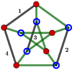
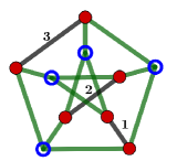
Figure 1. Anti-Cheeger cut (left) v.s. maxcut (right) on the Petersen graph: A bipartition $(S,S^{\prime})$ of the vertex set $V$ is displayed in red bullets ($S$) and blue circles ($S^{\prime}$). For the anti-Cheeger cut, we have $\operatorname*{cut}(S)=11$, $\mathrm{vol}(S)=\mathrm{vol}(S^{\prime})=15$, $h_{\mathrm{anti}}(G)=\frac{11}{15}$, and the remaining four uncut edges are divided equally in $S$ and $S^{\prime}$ (judicious!). For the maxcut, we have $\operatorname*{cut}(S)=12$, $\mathrm{vol}(V)=30$, $h_{\max}(G)=\frac{12}{15}$, but the remaining three uncut edges are all contained in $S$ (biased!).

Recently, it has been shown that a set-pair Lovász extension produces some kinds of equivalent continuous optimization formulations for graph cut problems [CSZZ18]. The anti-Cheeger cut and maxcut problem (1.2) can be respectively rewritten into

(1.5) $$h_{\mathrm{anti}}(G) =\max_{\mbox{\boldmath$x$}\in\mathbb{R}^{n}\setminus\{\mbox{\boldmath$0$}\}}\frac{I(\mbox{\boldmath$x$})}{2\mathrm{vol}(V)\|\mbox{\boldmath$x$}\|_{\infty}-N(x)},$$

(1.6) $$h_{\max}(G) =\max_{\mbox{\boldmath$x$}\in\mathbb{R}^{n}\setminus\{\mbox{\boldmath$0$}\}}\frac{I(\mbox{\boldmath$x$})}{\mathrm{vol}(V)\|\mbox{\boldmath$x$}\|_{\infty}},$$

where

(1.7) $$I(\mbox{\boldmath$x$}) =\sum_{\{i,j\}\in E}w_{ij}|x_{i}-x_{j}|,$$

(1.8) $$N(\mbox{\boldmath$x$}) =\min_{c\in\mathbb{R}}\sum_{i=1}^{n}d_{i}|x_{i}-c|,$$

(1.9) $$\|\mbox{\boldmath$x$}\|_{\infty} =\max\{|x_{1}|,\ldots,|x_{n}|\}.$$

Comparing Eq. (1.5) with Eq. (1.6), it can be easily observed that the bias of maxcut is fixed by $N(\mbox{\boldmath$x$})$ in the anti-Cheeger cut using the fact that

(1.10) $$\alpha=\operatorname*{arg\,min}_{c\in\mathbb{R}}\sum_{i=1}^{n}d_{i}|x_{i}-c|\leavevmode\nobreak\ \leavevmode\nobreak\ \leavevmode\nobreak\ \text{ if and only if }\leavevmode\nobreak\ \leavevmode\nobreak\ \leavevmode\nobreak\ \alpha\in\mathrm{median}(\mbox{\boldmath$x$}),$$

where $\mathrm{median}(\mbox{\boldmath$x$})$ gives a range of the middle volume based on the order of $x$ (see Definition 1.3 and Lemma 2.3 in [CSZ15]). We can also derive from the above fact that $N(\mbox{\boldmath$x$})\leq\mathrm{vol}(V)||\mbox{\boldmath$x$}||_{\infty}$ and thus the objective function in Eq. (1.5) is positive. Actually, if the equality holds in Eq. (1.4), then there exists at least one maxcut, denoted by ${S_{*}}$ in Eq.  (1.3) or $\mbox{\boldmath$x$}_{*}$ in Eq. (1.6), satisfying $N(\mbox{\boldmath$x$}_{*})=\mathrm{vol}(V)||\mbox{\boldmath$x$}_{*}||_{\infty}$ which gives nothing but the perfect balance: $\mathrm{vol}(S_{*})=\mathrm{vol}(S_{*}^{c})=\frac{1}{2}\mathrm{vol}(V)$. Just starting from the equivalent continuous formulation (1.6), a simple iterative (SI) algorithm was proposed for solving the maxcut problem [SZZ18]. The numerical maxcut solutions obtained by SI on G-set are of comparable quality to those by advanced heuristic combinational algorithms and have the best cut values among all existing continuous algorithms. In view of the similarity between Eqs. (1.5) and (1.6), it is then legitimate to ask whether we are able to get the same good performance when a similar idea to SI is applied into the former. We will give an affirmative answer in this work.

The first step to develop a continuous iterative algorithm (CIA) from the fractional form (1.5) is to use the idea of Dinkelbach’s iteration [Din67], with which we can equivalently convert the quotient into a difference of two convex functions. By linearizing the function to be subtracted (see $Q_{r}(\mbox{\boldmath$x$})$ in Eq. (2.1b)) via its subgradient, it is further relaxed to a convex subproblem, the solution of which has an analytical expression. That is, we are able to still have a kind of SI algorithm for the anti-Cheeger cut. However, the selection of subgradient becomes more complicated than that for the maxcut because $Q_{r}(\mbox{\boldmath$x$})$ involves not only $I(\mbox{\boldmath$x$})$ for calculating the cut values, which is also exactly the function to be subtracted in the maxcut problem (1.6), but also $N(\mbox{\boldmath$x$})$ for measuring the judiciousness and the objective function value $r$. We cannot expect a satisfactory performance along with an arbitrary subgradient in $\partial Q_{r}(\mbox{\boldmath$x$})$. For instance, CIA0, our first iterative algorithm, constructs the subgradient in $\partial Q_{r}(\mbox{\boldmath$x$})$ with another two subgradients, one chosen from $\partial I(\mbox{\boldmath$x$})$ and the other $\partial N(\mbox{\boldmath$x$})$, which are independent of each other, and produces numerical solutions with poor quality. When the results obtained with a parallel evolutionary algorithm [SY21] on G-set are set to be the reference, the numerical lower bound of the ratios between the object function values achieved by CIA0 and the reference ones are only about $0.870$. To improve it, a careful subgradient selection is then designed and the resulting iterative algorithm is named CIA1, which increases the above numerical lower bound to $0.942$. We also show that CIA1 may get enough increase at each step (see Theorem 3.1) and converges to a local optimum (see Theorem 3.2).

Finally, in order to make further improvement in solution quality by jumping out of local optima of CIA1, we continue to exploit the similarity between Eqs. (1.5) and (1.6), which shares a common numerator $I(\mbox{\boldmath$x$})$ for the cut values. Specifically, once CIA1 cannot increase the objective function value for some successive iterative steps, we switch to the SI iterations for the maxcut and denote the resulting algorithm by CIA2. Preliminary numerical experiments show that the ratios between the object function values and the reference ones can be increased by CIA2 to at least $0.991$.

The paper is organized as follows. Section 2 presents three continuous iterative algorithms: CIA0, CIA1 and CIA2. Local convergence of CIA1 is established in Section 3. Numerical experiments on G-set are performed in Section 4. We are concluded with a few remarks in Section 5.

Acknowledgements. This research was supported by the National Natural Science Foundation of China (No. 11822102). SS is partially supported by Beijing Academy of Artificial Intelligence (BAAI). The authors would like to thank Dr. Weixi Zhang for helpful discussions and useful comments.

2. Iterative algorithms

Let $F(\mbox{\boldmath$x$})$ denote the continuous, positive and fractional objective function of the anti-Cheeger cut problem (1.5). Considering the zeroth order homogeneousness of $F(\mbox{\boldmath$x$})$, i.e., $F(\lambda\mbox{\boldmath$x$})\equiv F(\mbox{\boldmath$x$})$ holds for arbitrary $\lambda>0$, it suffices to search for a maximizer of $F(\mbox{\boldmath$x$})$ on a closed, bounded and connected set $\Omega:=\{\mbox{\boldmath$x$}\in\mathbb{R}^{n}\big{|}\|\mbox{\boldmath$x$}\|_{p}=1\}$, which can be readily achieved by the the following Dinkelbach iteration [Din67, SZZ18]

where

(2.1b) $$Q_{r}(\mbox{\boldmath$x$}) =\frac{I(\mbox{\boldmath$x$})+rN(\mbox{\boldmath$x$})}{2\mathrm{vol}(V)},\quad r\geq 0,$$

(2.1c) $$\|\mbox{\boldmath$x$}\|_{p} =(|x_{1}|^{p}+|x_{2}|^{p}+\cdots+|x_{n}|^{p})^{\frac{1}{p}},\quad p\geq 1.$$

Here we only need the intersection of $\Omega$ and any ray out from the original point is not empty and thus the choice of $p$ does not matter.

For any vector $\mbox{\boldmath$x$}^{*}$ reaching the maximum of $F(\mbox{\boldmath$x$})$, there exists $\hat{\mbox{\boldmath$x$}}\in M(\mbox{\boldmath$x$}^{*})$ such that

(2.1d) $$\frac{\hat{\mbox{\boldmath$x$}}}{||\hat{\mbox{\boldmath$x$}}||_{\infty}}=\mbox{\boldmath$1$}_{S^{*}}-\mbox{\boldmath$1$}_{(S^{*})^{c}}$$

also maximizes $F(\mbox{\boldmath$x$})$ on $\mbox{\boldmath$x$}\in\mathbb{R}^{n}\setminus\{\mbox{\boldmath$0$}\}$ thanks to the zeroth order homogeneousness of $F(\mbox{\boldmath$x$})$, where $S^{*}$ satisfies $S^{+}(\mbox{\boldmath$x$}^{*})\subset S^{*}\subset(S^{-}(\mbox{\boldmath$x$}^{*}))^{c}$. Therefore, $(S^{*},(S^{*})^{c})$ is an anti-Cheeger cut for graph $G$. Here $M(\mbox{\boldmath$x$}^{*})=\{\mbox{\boldmath$x$}\big{|}||\mbox{\boldmath$x$}||_{\infty}=||\mbox{\boldmath$x$}^{*}||_{\infty},S^{\pm}(\mbox{\boldmath$x$}^{*})\subseteq S^{\pm}(\mbox{\boldmath$x$})\}$, and $S^{\pm}(\mbox{\boldmath$x$})=\{i\in V\big{|}x_{i}=\pm||\mbox{\boldmath$x$}||_{\infty}\}$.

However, Eq (LABEL:iter0-1) is still a non-convex problem and can be further relaxed to a convex one by using the fact that, for any convex and first degree homogeneous function $f(\mbox{\boldmath$x$})$, we have

(2.1e) $$f(\mbox{\boldmath$x$})\geq(\mbox{\boldmath$x$},\mbox{\boldmath$s$}),\,\,\,\forall\,\mbox{\boldmath$s$}\in\partial f(\mbox{\boldmath$y$}),\,\,\,\forall\,\mbox{\boldmath$x$},\mbox{\boldmath$y$}\in\mathbb{R}^{n},$$

where $(\cdot,\cdot)$ denotes the standard inner product in $\mathbb{R}^{n}$ and $\partial f(\mbox{\boldmath$y$})$ gives the subgradient of function $f$ at $y$.

Using the relaxation (2.1e) in Eq. (LABEL:iter0-1) in view of that $Q_{r}(\mbox{\boldmath$x$})$ is convex and homogeneous of degree one, we then modify the two-step Dinkelbach iterative scheme (2.1) into the following three-step one

(2.1fa) $$\mbox{\boldmath$x$}^{k+1}=\operatorname*{arg\,min}\limits_{\|\mbox{\boldmath$x$}\|_{p}=1}\{r^{k}\|\mbox{\boldmath$x$}\|_{\infty}-(\mbox{\boldmath$x$},\mbox{\boldmath$s$}^{k})\},$$

(2.1fb) $$r^{k+1}=F(\mbox{\boldmath$x$}^{k+1}),$$

(2.1fc) $$\mbox{\boldmath$s$}^{k+1}\in\partial Q_{r^{k+1}}(\mbox{\boldmath$x$}^{k+1}),$$

with an initial data: $\mbox{\boldmath$x$}^{0}\in\mathbb{R}^{n}\setminus\{\mbox{\boldmath$0$}\}$, $r^{0}=F(\mbox{\boldmath$x$}^{0})$ and $\mbox{\boldmath$s$}^{0}\in\partial(Q_{r^{0}}(\mbox{\boldmath$x$}^{0}))$.

The iterative algorithm (2.1f) is called to be simple in [SZZ18] because the inner subproblem (2.1fa) has an analytical solution. That is, no any other optimization solver is needed in such simple three-step iteration. For the sake of completeness and the selection of subgradient in Eq. (2.1fc), we will write down the expression and some properties of the analytical solution and leave out all the proof details which can be found in [SZZ18].

Proposition 2.1 (Lemma 3.1 and Theorem 3.5 in [SZZ18]).

Suppose $\mbox{\boldmath$x$}^{k}$, $r^{k}$ and $\mbox{\boldmath$s$}^{k}$ are generated by the simple iteration (2.1f). Then for $k\geq 1$, we always have $0\leq r^{k-1}\leq r^{k}\leq\|\mbox{\boldmath$s$}^{k}\|_{1}$. In particular, (1) $r^{k}=\|\mbox{\boldmath$s$}^{k}\|_{1}$ if and only if $\mbox{\boldmath$x$}^{k}/\|\mbox{\boldmath$x$}^{k}\|_{\infty}\in\mathrm{Sgn}(\mbox{\boldmath$s$}^{k})$; and (2) $r^{k}<\|\mbox{\boldmath$s$}^{k}\|_{1}$ if and only if $L(r^{k},\mbox{\boldmath$s$}^{k})<0$. Here

(2.1g) $${L}(r,\mbox{\boldmath$v$})=\min_{\|\mbox{\boldmath$x$}\|_{p}=1}\{r\|\mbox{\boldmath$x$}\|_{\infty}-(\mbox{\boldmath$x$},\mbox{\boldmath$v$})\},\,\,\,r\in\mathbb{R},\,\,\mbox{\boldmath$v$}\in\mathbb{R}^{n},$$

denotes the minimal value of (2.1fa) and $\mathrm{Sgn}(\mbox{\boldmath$x$})=\{(s_{1},s_{2},\ldots,s_{n})\big{|}s_{i}\in\mathrm{Sgn}(x_{i}),\,i=1,2,\ldots,n\}$ with

(2.1h) $$\mathrm{Sgn}(t)=\begin{cases}\{1\},&\;\text{if }t>0,\\ \{-1\},&\;\text{if }t<0,\\ [-1,1],&\;\text{if }t=0.\end{cases}$$

Proposition 2.2 (Theorem 3.3 and Corollary 3.4 in [SZZ18]).

Let $\mbox{\boldmath$x$}^{*}$ be the solution of the minimization problem:

$$\mbox{\boldmath$x$}^{*}=\operatorname*{arg\,min}_{\|\mbox{\boldmath$x$}\|_{p}=1}\{r\|\mbox{\boldmath$x$}\|_{\infty}-(\mbox{\boldmath$x$},\mbox{\boldmath$v$})\}$$

under the condition $0<r\leq\|\mbox{\boldmath$v$}\|_{1}$. Without loss of generality, we assume $|v_{1}|\geq|v_{2}|\geq\ldots\geq|v_{n}|\geq|v_{n+1}|=0$, and define $m_{0}=\min\{m\in\{1,2,\ldots,n\}:A(m)>r\}$ and $m_{1}=\max\{m\in\{1,2,\ldots,n\}:A(m-1)<r\}$ with $A(m)=\sum_{j=1}^{m}(|v_{j}|-|v_{m+1}|)$.

Scenario 1:

For $r<||\mbox{\boldmath$v$}||_{1}$ and $1<p<\infty$, we have $\mbox{\boldmath$x$}^{*}=\frac{\mathrm{sign}(\mbox{\boldmath$v$})\mbox{\boldmath$z$}^{*}}{||\mbox{\boldmath$z$}^{*}||_{p}}$, where $\mbox{\boldmath$z$}^{*}=(z_{1},z_{2},\ldots,z_{n})$ with $z_{i}^{*}=\min\left\{1,\left(\frac{m_{0}|v_{i}|}{\sum_{j=1}^{m_{0}}|v_{j}|-r}\right)^{\frac{1}{p-1}}\right\}$.

Scenario 2:

For $r<||\mbox{\boldmath$v$}||_{1}$ and $p=1$, we have $\mbox{\boldmath$x$}^{*}=\frac{\mathrm{sign}(\mbox{\boldmath$v$})\mbox{\boldmath$z$}^{*}}{||\mbox{\boldmath$z$}^{*}||_{p}}$, where

$$z_{i}^{*}=\left\{\begin{aligned} &1,&1\leq i\leq m_{1},\\ &0,&m_{0}\leq i\leq n,\\ &[0,1],&m_{1}<i<m_{0}.\end{aligned}\right.$$

Scenario 3:

For $r=||\mbox{\boldmath$v$}||_{1}$ or $p=\infty$, the solution $\mbox{\boldmath$x$}^{*}$ satisfies $\frac{\mbox{\boldmath$x$}^{*}}{||\mbox{\boldmath$x$}^{*}||_{\infty}}\in\mathrm{Sgn}(\mbox{\boldmath$v$})$ and $||\mbox{\boldmath$x$}^{*}||_{p}=1$.

Moreover, the minimizer $\mbox{\boldmath$x$}^{*}$ satisfies

(2.1i) $$\frac{(\mbox{\boldmath$x$}^{*},\mbox{\boldmath$v$})}{\|\mbox{\boldmath$x$}^{*}\|_{\infty}}\geq\sum_{i=1}^{m}|v_{i}|,$$

where $m=m_{0}$ for both Scenario 1 and Scenario 2, and $m=n$ for Scenario 3.

The only thing remaining is to figure out the subgradient in Eq. (2.1fc). Using the linear property of subgradient, we have

(2.1j) $$\partial Q_{r}(\mbox{\boldmath$x$})=\frac{1}{2\mathrm{vol}(V)}\left(\partial I(\mbox{\boldmath$x$})+r\partial N(\mbox{\boldmath$x$})\right),$$

which means we may construct $\mbox{\boldmath$s$}\in\partial Q_{r}(\mbox{\boldmath$x$})$ through $\mbox{\boldmath$u$}\in\partial I(\mbox{\boldmath$x$})$ and $\mbox{\boldmath$v$}\in\partial N(\mbox{\boldmath$x$})$ as

(2.1k) $$\mbox{\boldmath$s$}=\frac{1}{2\mathrm{vol}(V)}\left(\mbox{\boldmath$u$}+r\mbox{\boldmath$v$}\right).$$

It was suggested in [SZZ18] to use a point, denoted by $\bar{\mbox{\boldmath$p$}}=(\bar{p}_{1},\ldots,\bar{p}_{n})$, located on the boundary of $\partial I(\mbox{\boldmath$x$})$ as an indicator for selecting $\mbox{\boldmath$u$}\in\partial I(\mbox{\boldmath$x$})$ to solve the maxcut problem (1.6), where

$$\bar{p}_{i} =\left\{\begin{array}[]{ll}{p_{i}\mp q_{i},}&{\text{ if }i\in S^{\pm}(\mbox{\boldmath$x$}),}\\ {p_{i}+\operatorname{sign}\left(p_{i}\right)q_{i},}&{\text{ if }i\in S^{<}(\mbox{\boldmath$x$}),}\end{array}\right.$$

$$p_{i} =\sum_{j:\{i,j\}\in E}w_{ij}\mathrm{sign}(x_{i}-x_{j})-q_{i},\quad q_{i}=\sum_{j:\{i,j\}\in E\text{ and }x_{i}=x_{j}}w_{ij},$$

$$\mathrm{sign}(t) =\begin{cases}1,&\;\text{if }t\geq 0,\\ -1,&\;\text{if }t<0,\end{cases}\quad\text{and}\quad S^{<}(\mbox{\boldmath$x$})=\{i\in V\big{|}|x_{i}|<||\mbox{\boldmath$x$}||_{\infty}\}.$$

It tries to select the boundary point at each dimension with the help of a partial order relation ‘$\leq$’ on $\mathbb{R}^{2}$ by $(x_{1},y_{1})\leq(x_{2},y_{2})$ if and only if either $x_{1}<x_{2}$ or $x_{1}=x_{2},y_{1}\leq y_{2}$ holds. Given a vector $\mbox{\boldmath$a$}=(a_{1},\ldots,a_{n})\in\mathbb{R}^{n}$, let $\Sigma_{\mbox{\boldmath$a$}}(\mbox{\boldmath$x$})$ be a collection of permutations of $\{1,2,\ldots,n\}$ such that for any $\sigma\in\Sigma_{\mbox{\boldmath$a$}}(\mbox{\boldmath$x$})$, it holds

$$(x_{\sigma(1)},a_{\sigma(1)})\leq(x_{\sigma(2)},a_{\sigma(2)})\leq\cdots\leq(x_{\sigma(n)},a_{\sigma(n)}).$$

Then for any $\sigma\in\Sigma_{\bar{\mbox{\boldmath$p$}}}(\mbox{\boldmath$x$})$, we select

(2.1l) $$\mbox{\boldmath$u$}=(u_{1},\ldots,u_{n})\in\partial I(\mbox{\boldmath$x$}),\quad u_{i}=\sum_{j:\{i,j\}\in E}w_{ij}\mathrm{sign}(\sigma^{-1}(i)-\sigma^{-1}(j))$$

$&$

It can be readily verified that $(\mbox{\boldmath$v$},\mbox{\boldmath$1$})=0$ for any $\mbox{\boldmath$v$}\in\partial N(\mbox{\boldmath$x$})$, and thus we may select

(2.1o) $$\mbox{\boldmath$v$}=(v_{1},\ldots,v_{n})\in\partial N(\mbox{\boldmath$x$}),\quad v_{i}=\left\{\begin{array}[]{ll}{d_{i}\mathrm{sign}(x_{i}-\alpha),}&{\text{ if }i\in V\backslash S^{\alpha}(\mbox{\boldmath$x$}),}\\ {\frac{A}{B}d_{i},}&{\text{ if }i\in S^{\alpha}(\mbox{\boldmath$x$}),}\end{array}\right.$$

where $\alpha\in\mathrm{median}(\mbox{\boldmath$x$})$, $S^{\alpha}(\mbox{\boldmath$x$})=\{i\in V\big{|}x_{i}=\alpha\}$, and

$$A=-\sum_{i\in V\backslash S^{\alpha}(\mbox{\boldmath$x$})}v_{i}=\sum_{x_{i}<\alpha}d_{i}-\sum_{x_{i}>\alpha}d_{i},\quad B=\sum_{i\in S^{\alpha}(\mbox{\boldmath$x$})}d_{i}=\sum_{x_{i}=\alpha}d_{i}.$$

Such selection of subgradient was already used to solve the Cheeger cut problem $h(G)=\min\limits_{S\subset V,S\not\in\{\varnothing,V\}}\frac{\operatorname*{cut}(S)}{\min\{\mathrm{vol}(S),\mathrm{vol}(S^{c})\}}$ in [CSZ15] in view of the equivalent continuous formulation $h(G)=\min\limits_{\mbox{\boldmath$x$}\leavevmode\nobreak\ \leavevmode\nobreak\ \mathrm{nonconstant}}\frac{I(\mbox{\boldmath$x$})}{N(\mbox{\boldmath$x$})}$ [CSZZ18].

With those selections in Eqs. (2.1l) and (2.1o) at our disposal, we immediately obtain the first continuous iterative algorithm (abbreviated as CIA0) after using Eq. (2.1k) in the three-step iteration (2.1f). Although it still keeps the monotone increasing $r^{k+1}\geq r^{k}$ as stated in Proposition 2.1, CIA0 may not have enough increase at every iteration step because the selected $\mbox{\boldmath$s$}\in\partial Q_{r}(\mbox{\boldmath$x$})$ is not located on the boundary of $\partial Q_{r}(\mbox{\boldmath$x$})$. The numerical results in Table 1 show clearly such unsatisfactory performance. Actually, according to Eq. (2.1i), the monotone increasing of $\{r^{k}\}_{k=1}^{\infty}$ has a direct connection to the subgradient $s$ as follows

(2.1p) $$r^{k+1}=\frac{Q_{r^{k+1}}(\mbox{\boldmath$x$}^{k+1})}{\|\mbox{\boldmath$x$}^{k+1}\|_{\infty}}\geq\frac{Q_{r^{k}}(\mbox{\boldmath$x$}^{k+1})}{\|\mbox{\boldmath$x$}^{k+1}\|_{\infty}}\geq\frac{(\mbox{\boldmath$x$}^{k+1},\mbox{\boldmath$s$}^{k})}{\|\mbox{\boldmath$x$}^{k+1}\|_{\infty}}\geq\sum_{i\in\iota}|s_{i}^{k}|\geq r^{k},$$

where there exists an index set $\iota\subset\{1,2,\ldots,n\}$, of which the size should be $m$ in Eq. (2.1i). In particular, such monotone increasing could be strict, i.e., $r^{k+1}>r^{k}$ via improving the last ‘$\geq$’ in Eq. (2.1p) into ‘$>$’, if $\|\mbox{\boldmath$s$}^{k}\|_{1}>r^{k}$ holds in each step. To this end, we only need to determine a subgradient $\mbox{\boldmath$s$}^{k}\in\partial Q_{r^{k}}(\mbox{\boldmath$x$}^{k})$ such that $\|\mbox{\boldmath$s$}^{k}\|_{1}>r^{k}$ if there exists $\mbox{\boldmath$s$}^{k}\in\partial Q_{r^{k}}(\mbox{\boldmath$x$}^{k})$ such that $\|\mbox{\boldmath$s$}^{k}\|_{1}>r^{k}$. That is, we should hunt $\mbox{\boldmath$s$}^{k}$ on the boundary of $\partial Q_{r^{k}}(\mbox{\boldmath$x$}^{k})$ after noting the convexity of the set $\partial Q_{r^{k}}(\mbox{\boldmath$x$}^{k})$ and the function $\|\cdot\|_{1}$.

We know that, if $|S^{\alpha}(\mbox{\boldmath$x$})|\leq 1$, $\partial N(\mbox{\boldmath$x$})$ contains just a single vector, denoted by $a$, which is given by Eq. (2.1o), too; otherwise, $(\partial N(\mbox{\boldmath$x$}))_{i}$ becomes an interval for $i\in S^{\alpha}(\mbox{\boldmath$x$})$, denoted by $[a_{i}^{L},a_{i}^{R}]$ with $a_{i}^{L}=\max\{A-B+d_{i},-d_{i}\}$ and $a_{i}^{R}=\min\{A+B-d_{i},d_{i}\}$. We still adopt a point $\mbox{\boldmath$b$}=(b_{1},\ldots,b_{n})\in\mathbb{R}^{n}$ on the boundary of $\partial Q_{r}(\mbox{\boldmath$x$})$ as an indicator for choosing $\mbox{\boldmath$u$}\in\partial I(\mbox{\boldmath$x$})$ and $\mbox{\boldmath$v$}\in\partial N(\mbox{\boldmath$x$})$ such that the resulting $s$ given by Eq. (2.1k) lives on the boundary of $\partial Q_{r}(\mbox{\boldmath$x$})$, and the discussion is accordingly divided into two cases below.

$\bullet\leavevmode\nobreak\ |S^{\alpha}(\mbox{\boldmath$x$})|\leq 1$:

For $i=1,2,\ldots,n$, let

(2.1s) $$b_{i}=\left\{\begin{array}[]{ll}{p_{i}\mp q_{i}+ra_{i},}&{\text{ if }i\in S^{\pm}(\mbox{\boldmath$x$}),}\\ {p_{i}+ra_{i}+\operatorname{sign}\left(p_{i}+ra_{i}\right)q_{i},}&\text{ if }i\in S^{<}(\mbox{\boldmath$x$}),\end{array}\right.$$

and then we select

(2.1t) $$u_{i} =\sum_{j:\{i,j\}\in E}w_{ij}\mathrm{sign}(\sigma^{-1}(i)-\sigma^{-1}(j)),\quad\sigma\in\Sigma_{\mbox{\boldmath$b$}}(\mbox{\boldmath$x$}),$$

(2.1u) $$v_{i} =a_{i}.$$

$\bullet\leavevmode\nobreak\ |S^{\alpha}(\mbox{\boldmath$x$})|\geq 2$:

For $i=1,2,\ldots,n$, let

(2.1v) $$a_{i} =\begin{cases}d_{i}\mathrm{sign}(x_{i}-\alpha),&\text{if $i\in V\setminus S^{\alpha}(\mbox{\boldmath$x$})$},\\ a^{L}_{i},&\text{if $i\in S^{\alpha}(\mbox{\boldmath$x$})\cap S^{+}(\mbox{\boldmath$x$})$},\\ a^{R}_{i},&\text{if $i\in S^{\alpha}(\mbox{\boldmath$x$})\cap S^{-}(\mbox{\boldmath$x$})$},\\ \displaystyle\operatorname*{arg\,max}_{t\in\{a^{L}_{i},a^{R}_{i}\}}\{|p_{i}+rt|\},&\text{if $i\in S^{\alpha}(\mbox{\boldmath$x$})\cap S^{<}(\mbox{\boldmath$x$})$},\end{cases}$$

(2.1y) $$b_{i} =\left\{\begin{array}[]{ll}{p_{i}\mp q_{i}+ra_{i},}&{\text{ if }i\in S^{\pm}(\mbox{\boldmath$x$}),}\\ {p_{i}+ra_{i}+\operatorname{sign}\left(p_{i}+ra_{i}\right)q_{i},}&{\text{ if }i\in S^{<}(\mbox{\boldmath$x$}).}\end{array}\right.$$

Given $\sigma\in\Sigma_{\mbox{\boldmath$b$}}(\mbox{\boldmath$x$})$ with the indicator $b$ determined by Eq. (2.1y), we choose $\mbox{\boldmath$u$}\in\partial I(\mbox{\boldmath$x$})$ according to Eq. (2.1t). Let $i^{*}$ be the first index satisfying $x_{\sigma(i^{*})}=\alpha$ and $i^{*}+t^{*}$ the last index satisfying $x_{\sigma(i^{*}+t^{*})}=\alpha$, i.e., $x_{\sigma(i^{*}-1)}<x_{\sigma(i^{*})}=x_{\sigma(i^{*}+1)}=\cdots=x_{\sigma(i^{*}+t^{*})}=\alpha<x_{\sigma(i^{*}+t^{*}+1)}$, and $j^{*}=\operatorname*{arg\,max}_{j\in\{\sigma(i^{*}),\sigma(i^{*}+t^{*})\}}\{|b_{j}|\}$. Then, we select

(2.1z) $$v_{i}=\begin{cases}a_{i},&\text{if }i\in V\backslash S^{\alpha}(\mbox{\boldmath$x$}),\\ a_{i},&\text{if }i\in S^{\alpha}(\mbox{\boldmath$x$})\cap S^{+}(\mbox{\boldmath$x$})\cap\{\sigma(i^{*})\},\\ \frac{A-a_{\sigma(i^{*})}}{B-d_{\sigma(i^{*})}}d_{i},&\text{if }i\in S^{\alpha}(\mbox{\boldmath$x$})\cap S^{+}(\mbox{\boldmath$x$})\backslash\{\sigma(i^{*})\},\\ a_{i},&\text{if }i\in S^{\alpha}(\mbox{\boldmath$x$})\cap S^{-}(\mbox{\boldmath$x$})\cap\{\sigma(i^{*}+t^{*})\},\\ \frac{A-a_{\sigma(i^{*}+t^{*})}}{B-d_{\sigma(i^{*}+t^{*})}}d_{i},&\text{if }i\in S^{\alpha}(\mbox{\boldmath$x$})\cap S^{-}(\mbox{\boldmath$x$})\backslash\{\sigma(i^{*}+t^{*})\},\\ a_{i},&\text{if }i\in S^{\alpha}(\mbox{\boldmath$x$})\cap S^{<}(\mbox{\boldmath$x$})\cap\{j^{*}\},\\ \frac{A-a_{j^{*}}}{B-d_{j^{*}}}d_{i},&\text{if }i\in S^{\alpha}(\mbox{\boldmath$x$})\cap S^{<}(\mbox{\boldmath$x$})\backslash\{j^{*}\}.\\ \end{cases}$$

Plugging the above selection of subgradient into the three-step iteration (2.1f) yields the second continuous iterative algorithm, named as CIA1 for short. It will be shown in next section that CIA1 is sufficient to get enough increase at every step (see Theorem 3.1) and converges to a local optima (see Theorem 3.2).

Figure 2. The flowchart of CIA2 — a continuous iterative algorithm for the anti-Cheeger cut equipped with breaking out of local optima by the maxcut. $F_{\text{anti}}(\mbox{\boldmath$x$})$ denotes the objective function of the anti-Cheeger cut problem (1.5) and $F_{\max}(\mbox{\boldmath$x$})$ the objective function of the maxcut problem (1.6). $T_{\text{tot}}$ gives the total iterative steps and $T_{=}$ counts the number of successive iterative steps in which the objective function values $F_{\text{anti}}(\mbox{\boldmath$x$})$ or $F_{\max}(\mbox{\boldmath$x$})$ keep unchanged.

In practice, CIA1 may converge fast to a local optimum (see e.g., Fig. 3), and thus need to cooperate with some local breakout techniques to further improve the solution quality. The similarity between the anti-Cheeger cut problem (1.5) and the maxcut problem (1.6), which shares a common numerator $I(\mbox{\boldmath$x$})$ for the cut values, provides a natural choice for us. We propose to switch to the SI iterations for the maxcut problem (1.6) when CIA1 cannot increase the objective function value for some successive iterative steps. The resulting iterative algorithm is denoted by CIA2, the flowchart of which is displayed in Fig. 2. It can be readily seen there that the maxcut iterations obtain an equal position with the anti-Cheeger cut iterations, which means CIA2 also improves the solution quality of the maxcut problem by using the anti-Cheeger cut to jump out of local optima at the same time. That is, the anti-Cheeger cut problem (1.5) and the maxcut problem (1.6) are fully treated on equal terms by CIA2.

3. Local convergence

We already figure out the selection of subgradient (CIA1) in the iterative scheme (2.1f), then we determine the selection of next solution $\mbox{\boldmath$x$}^{k+1}$ in Eq. (2.1fa). We choose the solution $\mbox{\boldmath$x$}^{k+1}\in\partial X_{p}^{k+1}$ in the same way as did in [SZZ18], where $X_{p}^{k+1}$ is the closed set of all the solutions $\mbox{\boldmath$x$}^{k+1}$, and $\partial X_{p}^{k+1}$ is the boundary of $\partial X_{p}^{k+1}\in X_{p}^{k+1}$. Thus, the three-step iterative scheme (2.1fa) of CIA1 can be clarified as

(2.1aa) $$\mbox{\boldmath$x$}^{k+1}\in\partial X_{p}^{k+1},$$

(2.1ab) $$r^{k+1}=F(\mbox{\boldmath$x$}^{k+1}),$$

(2.1ac) $$\mbox{\boldmath$s$}^{k+1}=\mbox{\boldmath$s$}^{\sigma},\,\,\,\sigma\in\Sigma_{\mbox{\boldmath$b$}}(\mbox{\boldmath$x$}^{k+1}).$$

Let

(2.1b) $$C=\{\mbox{\boldmath$x$}\in\mathbb{R}^{n}\big{|}F(\mbox{\boldmath$y$})\leq F(\mbox{\boldmath$x$}),\,\,\forall\,\mbox{\boldmath$y$}\in\{R_{i}\mbox{\boldmath$x$}:i\in\{1,\ldots,n\}\}\},$$

where $R_{i}\mbox{\boldmath$x$}$ is defined as

(2.1c) $$(R_{i}\mbox{\boldmath$x$})_{j}=\begin{cases}x_{j},&j\neq i,\\ -x_{j},&j=i.\end{cases}$$

The following two theorems verify two important properties of CIA1 in (2.1a). Theorem 3.1 and Proposition 2.1 imply that the sequence $\{r^{k}\}$ strictly increases when there exists $\mbox{\boldmath$s$}\in\partial Q_{r^{k}}(\mbox{\boldmath$x$}^{k})$ such that $\|\mbox{\boldmath$s$}\|_{1}>r^{k}$, of which the opposite statement is the necessary condition for the convergence of $\{r^{k}\}$. Theorem 3.2 guarantees the iterating scheme converges with $r^{k}=r^{*}$ and $\mbox{\boldmath$x$}^{k}=\mbox{\boldmath$x$}^{*}$ in finite steps, where $\mbox{\boldmath$x$}^{*}\in C$ is a local maximizer from the discrete point of view. Furthermore, we are able to prove that $\mbox{\boldmath$x$}^{*}$ is also a local maximizer in the neighborhood $U(\mbox{\boldmath$x$}^{*})$:

(2.1d) $$U(\mbox{\boldmath$x$}^{*})=\left\{\mbox{\boldmath$y$}\in\mathbb{R}^{n}\,\,\Big{|}\,\,\|\frac{\mbox{\boldmath$y$}}{\|\mbox{\boldmath$y$}\|_{\infty}}-\frac{\mbox{\boldmath$x$}^{*}}{\|\mbox{\boldmath$x$}^{*}\|_{\infty}}\|_{\infty}<\frac{1}{2}\right\}.$$

Theorem 3.1.

We have

$$\|\mbox{\boldmath$s$}^{\sigma}\|_{1}>r^{k},\,\forall\,\sigma\in\Sigma_{\mbox{\boldmath$b$}}(\mbox{\boldmath$x$}^{k}),$$

if and only if there exists $\mbox{\boldmath$s$}\in\partial Q_{r^{k}}(\mbox{\boldmath$x$}^{k})$ satisfying $\|\mbox{\boldmath$s$}\|_{1}>r^{k}$.

Proof.

The necessity is obvious, we only need to prove the sufficiency. Suppose we can select subgradient $\mbox{\boldmath$s$}=(s_{1},\ldots,s_{n})\in\partial Q_{r^{k}}(\mbox{\boldmath$x$}^{k})$ satisfying $\|\mbox{\boldmath$s$}\|_{1}>r^{k}$, which directly implies $\mbox{\boldmath$x$}^{k}/\|\mbox{\boldmath$x$}^{k}\|_{\infty}\notin\mathrm{Sgn}(\mbox{\boldmath$s$})$ according to Proposition 2.1. Accordingly, there exists an $i^{*}\in\{1,2,\ldots,n\}$ such that $x_{i^{*}}^{k}/\|\mbox{\boldmath$x$}^{k}\|_{\infty}\notin\mathrm{Sgn}(s_{i^{*}})$, and the corresponding component $s_{i^{*}}$ satisfies

(2.1e) $$\left\{\begin{aligned} &s_{i^{*}}<0,&\text{if }i^{*}\in S^{+}(\mbox{\boldmath$x$}^{k}),\\ &s_{i^{*}}>0,&\text{if }i^{*}\in S^{-}(\mbox{\boldmath$x$}^{k}),\\ &|s_{i^{*}}|>0,&\text{if }i^{*}\in S^{<}(\mbox{\boldmath$x$}^{k}),\\ \end{aligned}\right.$$

which implies

(2.1f) $$\left\{\begin{aligned} &u_{i^{*}}\geq p_{i^{*}}-q_{i^{*}},\,v_{i^{*}}\geq a_{i^{*}}\,\Rightarrow\,2\mathrm{vol}(V)s_{i^{*}}\geq b_{i^{*}},&\text{if }i^{*}\in S^{+}(\mbox{\boldmath$x$}^{k}),\\ &u_{i^{*}}\leq p_{i^{*}}-q_{i^{*}},\,v_{i^{*}}\leq a_{i^{*}}\,\Rightarrow\,2\mathrm{vol}(V)s_{i^{*}}\leq b_{i^{*}},&\text{if }i^{*}\in S^{-}(\mbox{\boldmath$x$}^{k}),\\ &|u_{i^{*}}+r^{k}v_{i^{*}}|\leq|b_{i^{*}}|\,\Rightarrow\,2\mathrm{vol}(V)|s_{i^{*}}|\leq|b_{i^{*}}|,&\text{if }i^{*}\in S^{<}(\mbox{\boldmath$x$}^{k}).\\ \end{aligned}\right.$$

Let $S^{=}_{i^{*}}(\mbox{\boldmath$x$}^{k})=\{i\big{|}x_{i}^{k}=x_{i^{*}}^{k}\}$, and $i_{1},i_{2}\in S^{=}_{i^{*}}(\mbox{\boldmath$x$}^{k})$ be the indexes minimizing and maximizing function $\sigma^{-1}(\cdot)$ over $S^{=}_{i^{*}}(\mbox{\boldmath$x$}^{k})$, respectively. Then, we have

$$s^{\sigma}_{i_{1}}= \frac{1}{2\mathrm{vol}(V)}\left(\sum_{t:\{t,i_{1}\}\in E}w_{i_{1}t}\mathrm{sign}(\sigma^{-1}(i_{1})-\sigma^{-1}(t))+r^{k}v_{i_{1}}\right)$$

$$= \frac{1}{2\mathrm{vol}(V)}\left(p_{i_{1}}-q_{i_{1}}+r^{k}v_{i_{1}}\right),$$

$$s^{\sigma}_{i_{2}}= \frac{1}{2\mathrm{vol}(V)}\left(\sum_{t:\{t,i_{2}\}\in E}w_{i_{2}t}\mathrm{sign}(\sigma^{-1}(i_{2})-\sigma^{-1}(t))+r^{k}v_{i_{2}}\right)$$

$$= \frac{1}{2\mathrm{vol}(V)}\left(p_{i_{2}}+q_{i_{2}}+r^{k}v_{i_{2}}\right),$$

and then the subgradient selection in Eqs. (2.1s)-(2.1z) yields

(2.1g) $$\left\{\begin{aligned} &s_{i_{1}}^{\sigma}=b_{i_{1}}\leq b_{i^{*}}\leq 2\mathrm{vol}(V)s_{i^{*}}<0,&\text{if }i^{*}\in S^{+}(\mbox{\boldmath$x$}^{k}),\\ &s_{i_{2}}^{\sigma}=b_{i_{2}}\geq b_{i^{*}}\geq 2\mathrm{vol}(V)s_{i^{*}}>0,&\text{if }i^{*}\in S^{-}(\mbox{\boldmath$x$}^{k}),\\ &\max\{|s_{i_{1}}^{\sigma}|,|s_{i_{2}}^{\sigma}|\}=\max\{|b_{i_{1}}|,|b_{i_{2}}|\}\geq|b_{i^{*}}|>0,&\text{if }i^{*}\in S^{<}(\mbox{\boldmath$x$}^{k}),\\ \end{aligned}\right.$$

where we have used Eq. (2.1f). Therefore, there exists $i\in\{i_{1},i_{2}\}$ satisfying $x_{i}^{k}/\|\mbox{\boldmath$x$}^{k}\|_{\infty}\notin\mathrm{Sgn}(s_{i}^{\sigma})$, and thus we have $||\mbox{\boldmath$s$}^{\sigma}||_{1}>r^{k}$ according to Proposition 2.1. ∎

Theorem 3.2 (finite-step local convergence).

Assume the sequences $\{\mbox{\boldmath$x$}^{k}\}$ and $\{r^{k}\}$ are generated by CIA1 in Eq. (2.1a) from any initial point $\mbox{\boldmath$x$}^{0}\in\mathbb{R}^{n}\setminus\{\mbox{\boldmath$0$}\}$. There must exist $N\in\mathbb{Z}^{+}$ and $r^{*}\in\mathbb{R}$ such that, for any $k>N$, $r^{k}=r^{*}$ and $\mbox{\boldmath$x$}^{k+1}\in C$ are local maximizers in $U(\mbox{\boldmath$x$}^{k+1})$.

Proof.

We first prove that the sequence $\{r^{k}\}$ takes finite values. It is obvious that for $p=1$, $p=\infty$ and $m=n$(one case in Eq. (2.1i)), we have

(2.1h) $$x^{k+1}_{i}/||\mbox{\boldmath$x$}^{k+1}||_{\infty}\in\{-1,0,1\},\quad\forall\,i=1,2,\ldots,n,$$

due to $\mbox{\boldmath$x$}^{k+1}\in\partial X_{p}^{k+1}$, and then $r^{k+1}(=F(\mbox{\boldmath$x$}^{k+1}))$ takes a limited number of values. In view of the fact that $\{r^{k}\}$ increases monotonically (see Proposition 2.1), there exists $N\in\mathbb{Z}^{+}$ and $r^{k}\in\mathbb{R}$ must take a certain value for $k>N$. That is, we only need to consider the remaining case for $1<p<\infty$ and $m<n$.

Suppose the contrary, we have that the subsequence $\{r^{k_{j}}\}_{j=1}^{\infty}\subset\{r^{k}\}_{k=1}^{\infty}$ increases strictly. According to Eq. (2.1p), there exists a permutation $\eta^{k_{j}}:\{1,2,\ldots,n\}\rightarrow\{1,2,\ldots,n\}$ satisfying

$$|s^{k_{j}}_{\eta^{k_{j}}(1)}|\geq|s^{k_{j}}_{\eta^{k_{j}}(2)}|\geq\ldots\geq|s^{k_{j}}_{\eta^{k_{j}}(n)}|,$$

then we have

(2.1i) $$r^{k_{j+1}}-r^{k_{j}}\geq r^{k_{j}+1}-r^{k_{j}}\geq\sum_{i=m+1}^{n}|s^{k_{j}}_{\eta^{k_{j}}(i)}|\geq|s_{\eta^{k_{j}}(m+1)}^{k_{j}}|.$$

If $s_{\eta^{k_{j}}(m+1)}^{k_{j}}=0$ holds for some $k_{j}$, then $\mbox{\boldmath$x$}^{k_{j}+1}$ satisfies Eq. (2.1h) derived from Scenario 1 of Proposition 2.2. Meanwhile, we also have $r^{k_{j}}=||\mbox{\boldmath$s$}^{k_{j}}||_{1}$, which implies $r^{k}=r^{k_{j}}$ for $k>k_{j}$. This is a contradiction. Therefore, we have $|s_{\eta^{k_{j}}(m+1)}^{k_{j}}|>0,\,\forall\,j\in\mathbb{N}$ for the subsequence $\{r^{k_{j}}\}_{j=1}^{\infty}$. The range of $\sum_{i\in\iota}|s_{i}^{k}|$ is

$$\left\{\sum_{i\in\iota}(a_{i}u_{i}+rh_{i}v_{i})\Big{|}\mbox{\boldmath$u$}^{\sigma}=(u_{1},\ldots,u_{n}),\,\mbox{\boldmath$v$}^{\sigma}=(v_{1},\ldots,v_{n}),\,\forall\,\sigma\in\Sigma_{\mbox{\boldmath$b$}}(\mbox{\boldmath$x$}),\,\forall\,\mbox{\boldmath$x$},\iota\right\},$$

which satisfies $\mbox{\boldmath$a$},\mbox{\boldmath$h$}\in\{-1,1\}^{n}$ and $a_{i}u_{i}+h_{i}v_{i}\geq 0,\,\,\forall\,i=1,2,\ldots,n$, Obviously, the choice of $u$, $v$, $a$, $h$ and $\eta^{k_{j}}$ are finite. Thus, there exists a subsequence $\{r^{k_{j_{t}}}\}_{t=1}^{\infty}\subset\{r^{k_{j}}\}_{j=1}^{\infty}$ satisfying that for any $t_{1},\,t_{2}\in\mathbb{Z}^{+}$, we have $\mbox{\boldmath$u$}^{k_{j_{t_{1}}}}=\mbox{\boldmath$u$}^{k_{j_{t_{2}}}}$, $\mbox{\boldmath$v$}^{k_{j_{t_{1}}}}=\mbox{\boldmath$v$}^{k_{j_{t_{2}}}}$, $\mbox{\boldmath$a$}^{k_{j_{t_{1}}}}=\mbox{\boldmath$a$}^{k_{j_{t_{2}}}}$, $\mbox{\boldmath$h$}^{k_{j_{t_{1}}}}=\mbox{\boldmath$h$}^{k_{j_{t_{2}}}}$ and $\eta^{k_{j_{t_{1}}}}=\eta^{k_{j_{t_{2}}}}$. Since $\{r^{k_{j_{t}}}\}_{t=1}^{\infty}$ increases monotonically, there exists $N_{0}\in\mathbb{Z}^{+}$, $\beta>0$ such that $|s_{\eta(m+1)}^{k_{j_{t}}}|>\beta$ for $t>N_{0}$, which contradicts to $r^{k_{j_{t}}}\leq 1,t\rightarrow\infty$ from Eq. (2.1i). Thus there exist $N\in\mathbb{Z}^{+}$ and $r^{*}\in\mathbb{R}$ such that $r^{k}=r^{*}$ for any $k>N$, thereby implying that

$$r^{k} =\|\mbox{\boldmath$s$}^{k}\|_{1},$$

$$X_{p}^{k+1} =\{\mbox{\boldmath$x$}\,\big{|}\,\mbox{\boldmath$x$}/\|\mbox{\boldmath$x$}\|_{\infty}\in\mathrm{Sgn}(\mbox{\boldmath$s$}^{k}),\,\,\|\mbox{\boldmath$x$}\|_{p}=1\},$$

derived from Proposition 2.1. That is, $\forall\,\mbox{\boldmath$x$}^{k+1}\in\partial X_{p}^{k+1}$, we have

(2.1j) $$\mbox{\boldmath$x$}^{k+1}/\|\mbox{\boldmath$x$}^{k+1}\|_{\infty} \in\mathrm{Sgn}(\mbox{\boldmath$s$}),\quad\forall\,s\in\partial Q_{r^{k}}(\mbox{\boldmath$x$}^{k+1}),$$

(2.1k) $$S^{<}(\mbox{\boldmath$x$}^{k+1}) =\varnothing.$$

Now we prove $\mbox{\boldmath$x$}^{k+1}\in C$ and neglect the superscript $k+1$ hereafter for simplicity. Suppose the contrary that there exists $i\in S^{\pm}(\mbox{\boldmath$x$})$ satisfying

(2.1l) $$F(R_{i}\mbox{\boldmath$x$})>F(\mbox{\boldmath$x$})\quad\Leftrightarrow\quad Q_{r^{k}}(R_{i}\mbox{\boldmath$x$})-Q_{r^{k}}(\mbox{\boldmath$x$})>0$$

because of $\|R_{i}\mbox{\boldmath$x$}\|_{\infty}=\|\mbox{\boldmath$x$}\|_{\infty}$.

On the other hand, we have

(2.1m) $$I(R_{i}\mbox{\boldmath$x$})-I(\mbox{\boldmath$x$})=\pm\sum\limits_{j:\{j,i\}\in E}2w_{ij}x_{j},\,\,i\in S^{\pm}(\mbox{\boldmath$x$}),$$

and

(2.1n) $$N(R_{i}\mbox{\boldmath$x$})-N(\mbox{\boldmath$x$})= -|\Delta-d_{i}x_{i}|+|\Delta+d_{i}x_{i}|$$

$$= \begin{cases}2d_{i}x_{i},&\text{if }\Delta>d_{i}||\mbox{\boldmath$x$}||_{\infty},\\ 2\Delta\mathrm{sign}(x_{i}),&\text{if }\Delta\leq d_{i}||\mbox{\boldmath$x$}||_{\infty},\\ -2d_{i}x_{i},&\text{if }\Delta<-d_{i}||\mbox{\boldmath$x$}||_{\infty},\end{cases}$$

from which, it can be derived that

(2.1o) $$\begin{cases}\mathrm{median}(\mbox{\boldmath$x$})=\mathrm{median}(R_{i}\mbox{\boldmath$x$})=\{1\},&\text{if }\Delta>d_{i}||\mbox{\boldmath$x$}||_{\infty},\\ x_{i}\in\mathrm{median}(\mbox{\boldmath$x$}),\,-x_{i}\in\mathrm{median}(R_{i}\mbox{\boldmath$x$}),&\text{if }\Delta\leq d_{i}||\mbox{\boldmath$x$}||_{\infty},\\ \mathrm{median}(\mbox{\boldmath$x$})=\mathrm{median}(R_{i}\mbox{\boldmath$x$})=\{-1\},&\text{if }\Delta<-d_{i}||\mbox{\boldmath$x$}||_{\infty},\end{cases}$$

where we have used the notation $\Delta:=\sum_{j=1}^{n}d_{j}x_{j}-d_{i}x_{i}$.

Let $\mbox{\boldmath$u$}=(u_{1},\ldots,u_{n})\in\partial I(\mbox{\boldmath$x$})$ with

$$u_{i}=\sum\limits_{j:\{j,i\}\in E}2w_{ij}z_{ij},\,\,\,z_{ij}=-x_{j}/\|\mbox{\boldmath$x$}\|_{\infty}\in\mathrm{Sgn}(x_{i}-x_{j}),$$

and $\mbox{\boldmath$v$}=(v_{1},\ldots,v_{n})\in\partial N(\mbox{\boldmath$x$})$ with

$$v_{i}=\begin{cases}-d_{i},&\text{if }\Delta>d_{i}||\mbox{\boldmath$x$}||_{\infty},\\ -\Delta\mathrm{sign}(x_{i}),&\text{if }\Delta\leq d_{i}||\mbox{\boldmath$x$}||_{\infty},\\ d_{i},&\text{if }\Delta<-d_{i}||\mbox{\boldmath$x$}||_{\infty}.\end{cases}$$

Combining Eqs. (2.1k), (2.1l) and (2.1o) together leads to

(2.1p) $$x_{i}s_{i}=\frac{x_{i}u_{i}+r^{k}x_{i}v_{i}}{2\mathrm{vol}(V)}<0,$$

which contradicts Eq. (2.1j).

Finally, we prove $x$ is a local maximizer of $F(\cdot)$ over $U(\mbox{\boldmath$x$})$. Let

$$\mbox{\boldmath$y$}^{\prime}=\frac{\|\mbox{\boldmath$x$}\|_{\infty}}{\|\mbox{\boldmath$y$}\|_{\infty}}\mbox{\boldmath$y$},\quad g(t)=Q_{F(\mbox{\boldmath$x$})}(t(\mbox{\boldmath$y$}^{\prime}-\mbox{\boldmath$x$})+\mbox{\boldmath$x$}),\quad\forall\,\mbox{\boldmath$y$}\in U(\mbox{\boldmath$x$}),$$

and we claim that

(2.1q) $$g(t)-g(0)\leq 0,\quad\forall\,t\in[0,1],$$

with which we are able to verify $x$ is a local maximizer as follows

$$F(\mbox{\boldmath$y$})-F(\mbox{\boldmath$x$})= F(\mbox{\boldmath$y$}^{\prime})-F(\mbox{\boldmath$x$})$$

$$= \frac{2\mathrm{vol}(V)}{2\mathrm{vol}(V)\|\mbox{\boldmath$y$}^{\prime}\|_{\infty}-N(\mbox{\boldmath$y$}^{\prime})}(Q_{F(\mbox{\boldmath$x$})}(\mbox{\boldmath$y$}^{\prime})-Q_{F(\mbox{\boldmath$x$})}(\mbox{\boldmath$x$}))$$

$$= \frac{2\mathrm{vol}(V)}{2\mathrm{vol}(V)\|\mbox{\boldmath$y$}^{\prime}\|_{\infty}-N(\mbox{\boldmath$y$}^{\prime})}(g(1)-g(0))\leq 0,\;\;\forall\,\mbox{\boldmath$y$}\in U(\mbox{\boldmath$x$}).$$

Now we only need to prove Eq. (2.1q). It is obvious that $g(t)$ is linear on $[0,1]$ and $||\mbox{\boldmath$y$}^{\prime}||_{\infty}=||\mbox{\boldmath$x$}||_{\infty}$, and there exists $\mbox{\boldmath$s$}=(s_{1},\ldots,s_{n})$ satisfying $\mbox{\boldmath$s$}\in\partial Q_{F(\mbox{\boldmath$x$})}(\mbox{\boldmath$x$})$ and $\mbox{\boldmath$s$}\in\partial Q_{F(\mbox{\boldmath$x$})}(\mbox{\boldmath$y$}^{\prime})$, which implies that $(\mbox{\boldmath$s$},\mbox{\boldmath$y$}^{\prime}-\mbox{\boldmath$x$})$ is the slope of $g(t)-g(0)$, i.e., $g(t)-g(0)=t(\mbox{\boldmath$s$},\mbox{\boldmath$y$}^{\prime}-\mbox{\boldmath$x$})$. With the fact that $\mathrm{sign}(\mbox{\boldmath$y$}^{\prime})=\mathrm{sign}(\mbox{\boldmath$x$})=\mathrm{sign}(\mbox{\boldmath$s$})$, we have

$$x_{j}(y^{\prime}_{j}-x_{j})\leq 0\Rightarrow s_{j}(y^{\prime}_{j}-x_{j})\leq 0,\quad j=1,2,\ldots,n,$$

then the claim Eq. (2.1q) is verified. ∎

Remark 3.3.

We would like to point out that the subgradient selection in CIA0 may not guarantee a similar local convergence, which can be verified in two steps. For the first step, numerical experiments show that the solutions produced by CIA0 on G-set are not contained in set $C$ with high probability. For the second step, we can prove that there exists $\mbox{\boldmath$y$}\in U(\mbox{\boldmath$x$})$ such that $F(\mbox{\boldmath$y$})>F(\mbox{\boldmath$x$})$ for any $\mbox{\boldmath$x$}\notin C$. The proof is briefed as follows. $\mbox{\boldmath$x$}\notin C$ implies that there exists $i\in S^{\pm}(\mbox{\boldmath$x$})$ such that $F(R_{i}\mbox{\boldmath$x$})>F(\mbox{\boldmath$x$})$, i.e., $Q_{F(\mbox{\boldmath$x$})}(R_{i}\mbox{\boldmath$x$})>Q_{F(\mbox{\boldmath$x$})}(\mbox{\boldmath$x$})$. Thus, according to Eq. (2.1p), there exists $\mbox{\boldmath$s$}\in\partial Q_{F(\mbox{\boldmath$x$})}(\mbox{\boldmath$x$})$ such that $x_{i}s_{i}<0$. Let $\mbox{\boldmath$y$}=(y_{1},\ldots,y_{n})\in\mathbb{R}^{n}$ with $y_{j}=x_{j}$ if $j\neq i$ and $y_{j}=\frac{x_{j}}{4}$ otherwise. It can be readily verified that $\mbox{\boldmath$y$}\in U(\mbox{\boldmath$x$})$, and

$$F(\mbox{\boldmath$y$})-F(\mbox{\boldmath$x$})= F(\mbox{\boldmath$y$}{\|\mbox{\boldmath$x$}\|_{\infty}}/{\|\mbox{\boldmath$y$}\|_{\infty}})-F(\mbox{\boldmath$x$})$$

$$= \frac{2\mathrm{vol}(V)}{2\mathrm{vol}(V)\|\mbox{\boldmath$y$}^{\prime}\|_{\infty}-N(\mbox{\boldmath$y$}^{\prime})}(g(1)-g(0))$$

$$= \frac{2\mathrm{vol}(V)}{2\mathrm{vol}(V)\|\mbox{\boldmath$y$}^{\prime}\|_{\infty}-N(\mbox{\boldmath$y$}^{\prime})}\cdot\left(-\frac{3x_{i}s_{i}}{4}\right)>0.$$

Table 1. Numerical results for the anti-Cheeger problem by continuous iterative algorithms on G-set. The objection function values obtained with a parallel evolutionary algorithm [SY21] are chosen to be the reference (see the second column). The third, fourth and fifth columns present the objection function values obtained with CIA0, CIA1 and CIA2, respectively. It can be easily seen that the numerical lower bound of the ratios between the object function values achieved by CIA0 and the reference ones are only about $0.870$ (see G36); and CIA1 improves it to $0.942$ (see G35), where we have chosen the maximum objection function values among $100$ runs from the same initial data and set the total iteration steps $T_{\text{tot}}=100$ for each run. Combined with a population updating manner, CIA2 further improves such numerical lower bound to $0.991$ (see G37), where we have set the population size $L=20$, $T_{=}=3$, and $T_{\text{tot}}=10000$. The last column counts the number of updating the population, denoted by $\#_{P}$. For instance, $\#_{P}=8$ for G37 means that CIA2 runs $\#_{P}\times L\times T_{\text{tot}}=8\times 20\times 10000=1600000$ iteration steps in total.

graph	reference values	numerical values (0)	numerical values (1)	numerical values (2)	$\#_{P}$
G1	0.6062	0.5764	0.5967	0.6031	2
G2	0.6059	0.5791	0.5943	0.6023	2
G3	0.6060	0.5716	0.5988	0.6049	2
G4	0.6073	0.5814	0.5970	0.6049	3
G5	0.6065	0.5836	0.5994	0.6050	2
G14	0.6524	0.5905	0.6264	0.6485	4
G15	0.6542	0.5951	0.6217	0.6486	5
G16	0.6533	0.5952	0.6213	0.6482	5
G17	0.6529	0.5869	0.6247	0.6473	7
G22	0.6682	0.6387	0.6554	0.6655	3
G23	0.6675	0.6381	0.6552	0.6642	3
G24	0.6671	0.6187	0.6551	0.6644	4
G25	0.6673	0.6358	0.6523	0.6627	3
G26	0.6667	0.6265	0.6503	0.6634	6
G35	0.6521	0.5713	0.6144	0.6463	12
G36	0.6520	0.5674	0.6157	0.6460	10
G37	0.6521	0.5865	0.6199	0.6460	8
G38	0.6525	0.5786	0.6192	0.6470	6
G43	0.6667	0.6422	0.6536	0.6645	3
G44	0.6657	0.6359	0.6533	0.6639	2
G45	0.6661	0.6352	0.6529	0.6623	3
G46	0.6655	0.6371	0.6530	0.6617	5
G47	0.6663	0.6265	0.6511	0.6631	6
G51	0.6510	0.5956	0.6248	0.6467	5
G52	0.6508	0.5935	0.6205	0.6471	6
G53	0.6507	0.5915	0.6264	0.6459	3
G54	0.6508	0.5866	0.6279	0.6471	5

4. Numerical experiments

In this section, we conduct performance evaluation of the proposed CIAs on the graphs with positive weight in G-set and always set the initial data $\mbox{\boldmath$x$}^{0}$ to be the maximal eigenvector of the graph Laplacian [DP93, PR95]. The three bipartite graphs $G48$, $G49$, $G50$ will not be considered because their optima cuts can be achieved at the initial step. The approximate solutions obtained with a parallel evolutionary algorithm are chosen to be the reference. Besides some extra work on calculating $N(\mbox{\boldmath$x$})$ and choosing $\mbox{\boldmath$v$}\in\partial N(\mbox{\boldmath$x$})$, both of which can be easily achieved by sorting, the detailed implementation of CIA0 and CIA1 is almost the same as that of SI for the maxcut problem, and so does the cost. In this regard, an anti-Cheeger iteration and a maxcut iteration, both adopted in CIA2 as shown in Fig. 2, are considered to have the same cost. The interested readers are referred to [SZZ18] for more details on the implementation and cost analysis, which are skipped here for simplicity. We have tried $p=1,2,\infty$ in Eq. (2.1fa) and found that, as we also expected in presenting the Dinkelbach iteration (2.1), the results for different $p$ $(=1,2,\infty)$ are comparable. Hence we only report the results for $p=1$ below.

We present the objection function values obtained with the proposed three kinds of CIAs in Table 1 and use a parallel evolutionary algorithm [SY21] to produce the reference values. In view of the unavoidable randomness in determining both $\mbox{\boldmath$x$}^{k+1}$ and $\mbox{\boldmath$s$}^{k+1}$, we re-run CIA0 (resp. CIA1) 100 times from the same initial data, and the third (resp. fourth) column of Table 1 records the maximum objection function values among these $100$ runs. We can see that the numerical lower bound of the ratios between the object function values achieved by CIA0 and the reference ones are only about $0.870$ (see G36); and CIA1 improves it to $0.942$ (see G35). That is, CIA1 has much better subgradient selection than CIA0, which has been already pointed out in Remark 3.3. Also with such careful selection of subgradient, CIA1 has a nice property of local convergence within finite steps as stated in Theorem 3.2. However, at the same time, it also means that CIA1 may converge fast to local optima and thus easily gets stuck in improving the solution quality further. This is clearly shown in Fig. 3 where we have plotted the history of the maximum objective function values chosen among 100 runs of CIA1 against the iterative steps on six typical graphs. In fact, CIA1 stops improving the solution quality after 53 steps for G1, 30 for G14, 25 for G22, 30 for G35, 17 for G43 and 39 for G51. This also explains why we choose a small $T_{\text{tot}}=100$ for both CIA0 and CIA1.

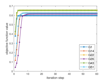
Figure 3. The maximum objective function value chosen among 100 runs of CIA1 from the same initial data v.s. iterative steps. We can clearly observe that CIA1 converges fast to a local optimum after a few iteration steps. It stops increasing the maximum objective function values (see the fourth column of Table 1) after 53 steps for G1, 30 for G14, 25 for G22, 30 for G35, 17 for G43 and 39 for G51.

Based on the similarity between the anti-Cheeger cut problem (1.5) and the maxcut problem (1.6), CIA2, the flowchart of which is given in Fig. 2, suggests a switch to the SI iterations for the latter when CIA1 cannot increase the objective function values of the former within $T_{=}$ successive iterative steps. Such switch can be considered to be a kind of local breakout technique for further improving the solution quality. We have implemented CIA2 in a population updating manner. In each round, the population contains $L$ numerical solutions, and its updating means precisely that $L$ independent CIA2 runs from the same initial data occur simultaneously. We record the numerical solution which achieves the maximum objective function value among these $L$ runs, adopt it as the initial data for the next round and define its objective function value to be the value of population. The population updating will not stop until the value of population keeps unchanged and we use $\#_{P}$ to count the number of such updating. After setting $L=20$ and $T_{=}=3$, the ratios between the maximum object function values (i.e., the final values of population, see the fifth column of Table 1) and the reference ones can be increased by CIA2 to at least $0.991$ (see G37), where a large $T_{\text{tot}}=10000$ is chosen to allow sufficient perturbations from local optima.

Table 1 shows evidently, on all 27 tested graphs, the objective function values produced by CIA2 are larger than those by CIA1, and the latter are larger than those by CIA0 as well. Moreover, the increased values from CIA2 to CIA1, which are obtained with breaking out of local optima by the maxcut, are usually less than those from CIA0 to CIA1, which are achieved with an appropriate subgradient selection. It should be pointed out that, CIA0 and CIA1 have the same cost, but the cost of the population implementation of CIA2 may be a little bit expensive in some occasions. Taking G37 as an example, CIA2 takes $\#_{P}\times L\times T_{\text{tot}}=1.6\times 10^{6}$ iteration steps in total to reach $0.6460$ (the ratio is $0.991$) while CIA2 only needs $100\times 100=10^{4}$ to reach $0.6199$ (the ratio is $0.951$). That is, an increase by four percentage points in the ratio costs about a hundredfold price. However, a good news is the population updating for CIA2 is a kind of embarrassingly parallel computation and thus can be perfectly accelerated with the multithreading technology.

5. Conclusion and outlook

Based on an equivalent continuous formulation, we proposed three continuous iterative algorithms (CIAs) for the anti-Cheeger cut problem, in which the objection function values are monotonically updated and all the subproblems have explicit analytic solutions. With a careful subgradient selection, we were able to prove the iteration points converge to a local optima in finite steps. Combined with the maxcut iterations for breaking out of local optima, the solution quality was further improved thanks to the similarity between the anti-Cheeger cut problem and the maxcut problem. The numerical solutions obtained by our CIAs on G-set are of comparable quality to those by an advanced heuristic combinational algorithm. We will continue to explore the intriguing mathematical characters and useful relations in both graph cut problems, and use them for developing more efficient algorithms.

References

- [CSZ15] K. C. Chang, S. Shao, and D. Zhang. The 1-laplacian cheeger cut: Theory and algorithms. J. Comput. Math., 33:443–467, 2015.
- [CSZZ18] K. C. Chang, S. Shao, D. Zhang, and W. Zhang. Lovász extension and graph cut. Commun. Math. Sci., to appear, 2021 (arXiv:1803.05257v3).
- [Din67] W. Dinkelbach. On nonlinear fractional programming. Manage. Sci., 13:492–498, 1967.
- [DP93] C. Delorme and S. Poljak. Laplacian eigenvalues and the maximum cut problem. Math. Program., 62:557–574, 1993.
- [Kar72] R. M. Karp. Reducibility among combinatorial problems. In R. E. Miller, J. W. Thatcher, and J. D. Bohlinger, editors, Complexity of Computer Computations, pages 85–103. Springer, 1972.
- [PR95] S. Poljak and F. Rendl. Solving the max-cut problem using eigenvalues. Discrete Appl. Math., 62:249–278, 1995.
- [SY21] S. Shao and C. Yang. A parallel evolutionary algorithm framework for graph cut problems. to be submitted, 2021.
- [SZZ18] S. Shao, D. Zhang, and W. Zhang. A simple iterative algorithm for maxcut. arXiv:1803.06496v2, 2018.
- [Xu16] B. Xu. Graph partitions: Recent progresses and some open problems. Adv. Math. (China), 45:1–20, 2016.