Learning an optimal feedback operator semiglobally stabilizing semilinear parabolic equations

Abstract.

Stabilizing feedback operators are presented which depend only on the orthogonal projection of the state onto the finite-dimensional control space. A class of monotone feedback operators mapping the finite-dimensional control space into itself is considered. The special case of the scaled identity operator is included. Conditions are given on the set of actuators and on the magnitude of the monotonicity, which guarantee the semiglobal stabilizing property of the feedback for a class semilinear parabolic-like equations. Subsequently an optimal feedback control minimizing the quadratic energy cost is computed by a deep neural network, exploiting the fact that the feedback depends only on a finite dimensional component of the state. Numerical simulations demonstrate the stabilizing performance of explicitly scaled orthogonal projection feedbacks, and of deep neural network feedbacks.

1. Introduction

We consider evolutionary semilinear parabolic-like equations, for time $t\geq 0$, as

$$\dot{y}+Ay+A_{\rm rc}y+{\mathcal{N}}(y)=0,\qquad y(0)=y_{0},$$ (1.1)

evolving in a Hilbert space $H$, where $A$ and $A_{\rm rc}=A_{\rm rc}(t)$ are a time-independent linear diffusion-like operator and a time-dependent linear reaction-convection-like operator. Further, ${\mathcal{N}}={\mathcal{N}}(t)$ is a time-dependent nonlinear operator for which conditions will be chosen so that existence and uniqueness of weak solutions for system (1.1) hold true for sufficiently small time $t\in[0,\tau)$, $0<\tau\leq+\infty$.

System (1.1) can be unstable, meaning that the norm $\left|y(t)\right|_{H}$ of its solution may diverge exponentially to $+\infty$ as $t\to\tau^{-}$. This motivates the investigation of feedback stabilization of (1.1). We shall concentrate on the case where this can be achieved by finitely many actuators.

Our first goal consists in semiglobal exponential stabilization of the system. More precisely, for arbitrary $R>0$ and $\mu>0$, we will prove that for a suitable $\lambda>0$, a set of actuators

$${U_{M}}\coloneqq\{\Phi_{j}\mid 1\leq j\leq M_{\sigma}\}\subset H,\qquad{\mathcal{U}}_{M}\coloneqq\mathop{\rm span}\nolimits U_{M},\qquad\dim{{\mathcal{U}}_{M}}=M_{\sigma},$$

with $M_{\sigma}\in\mathbb{N}$, and a suitable (possibly, time-dependent) feedback operator ${\mathcal{K}}_{M}(t,\raisebox{-1.07639pt}{\scalebox{1.25}{$\cdot$}})\colon{\mathcal{U}}_{M}\to{\mathcal{U}}_{M}$, the solution of

$$\dot{y}+Ay+A_{\rm rc}y+{\mathcal{N}}(y)={\mathcal{K}}_{M}(t,P_{{\mathcal{U}}_{M}}y),\color[rgb]{0,0,0}\qquad y(0)=y_{0},$$ (1.2)

satisfies

$$\left|y(t)\right|_{H}\leq\mathrm{e}^{-\mu(t-s)}\left|y(s)\right|_{H},\quad\mbox{for all}\quad t\geq s\geq 0\quad\mbox{and all}\quad y_{0}\in H\quad\mbox{with}\quad\left|y_{0}\right|_{H}<R.$$ (1.3)

Above, $M_{\sigma}=\sigma(M)$ is a strictly increasing sequence of positive integers. Note that at each instant of time the control input is a linear combination of the actuators in the form

$${\mathcal{K}}_{M}(t,P_{{\mathcal{U}}_{M}}y(t))=\textstyle\sum\limits_{j=1}^{M_{\sigma}}u_{j}(t)\Phi_{j},$$ (1.4)

for  $(u_{1}(t),u_{2}(t),\cdots,u_{M_{\sigma}}(t))\in{\mathbb{R}}^{M_{\sigma}}$.

Remark 1.1.

For the moment the reader may think of $M_{\sigma}=M$. The reason we consider a general subsequence $M_{\sigma}=\sigma(M)$ is due to the fact that in applications of the theoretical results to concrete examples of parabolic equations it is more convenient to have a result stated for a general subsequence, as we will see later in Section 5 where we will take the subsequence $M_{\sigma}=\sigma(M)=M^{d}$, for a parabolic equation evolving in a rectangular spatial domain $\Omega\subset{\mathbb{R}}^{d}$.

Definition 1.2.

For a given time-dependent operator ${\mathcal{K}}_{M}(t,\raisebox{-1.07639pt}{\scalebox{1.25}{$\cdot$}})\colon{\mathcal{U}}_{M}\to{\mathcal{U}}_{M}$, we write ${\mathcal{K}}_{M}\preceq-\overline{\lambda}{\mathbf{1}}$, if the inequality $({\mathcal{K}}_{M}(t,p),p)_{H}\leq-\overline{\lambda}\left|p\right|_{H}^{2}$ holds for every $p\in{\mathcal{U}}_{M}$, and almost every $t>0$.

We consider a general class of feedback laws in the form ${\mathcal{K}}_{M}\circ P_{{\mathcal{U}}_{M}}$, satisfying

$${\mathcal{K}}_{M}:[0,\infty)\times{\mathcal{U}}_{M}\to{\mathcal{U}}_{M},\quad {\mathcal{K}}_{M}(t,\raisebox{-1.07639pt}{\scalebox{1.25}{$\cdot$}})\in{\mathcal{C}}({\mathcal{U}}_{M},{\mathcal{U}}_{M}),$$ (1.5a)

$${\mathcal{K}}_{M}(t,0)=0,\quad {\mathcal{K}}_{M}(t,\cdot)\preceq-\overline{\lambda}{\mathbf{1}},\quad\overline{\lambda}>0.$$ (1.5b)

Under suitable assumptions on $(A,A_{\rm rc},{\mathcal{N}},{\mathcal{U}}_{M})$ and an extra regularity assumption on ${\mathcal{K}}_{M}$, which will be precised in Section 2 we will have the following result.

Main Result.

Let $R>0$, and $\mu>0$ be given. Let ${\mathcal{K}}_{M}\leq-\overline{\lambda}{\mathbf{1}}$. Then, if $M\in{\mathbb{N}}_{0}$ and $\overline{\lambda}>0$ are large enough, the solution of (1.2) satisfies (1.3) In particular, $t\mapsto\left|y(t)\right|_{H}$ is strictly decreasing at time $t=s$, if $\left|y(s)\right|_{H}\neq 0$.

Note also that the operator ${\mathcal{K}}_{M}(t,\cdot)$ in (1.5) may be nonlinear. We give now examples of such operators which are linear. The simplest class of such feedbacks consists of the scaled identity operator: for each $\lambda>0$, the operator

$$\breve{\mathcal{K}}_{M}^{\lambda}\coloneqq-\lambda{\mathbf{1}},$$ (1.6)

is in the class (1.5) above with $\overline{\lambda}=\lambda$, since $(\breve{\mathcal{K}}_{M}^{\lambda}(t,p),p)_{H}=-\lambda\left|p\right|_{H}^{2}$.

A second class of examples consists, as we shall see in Section 3.4, of the operators

$${\mathcal{K}}_{M}^{\lambda,\rho}\coloneqq-\lambda P_{{\mathcal{U}}_{M}}^{\widetilde{\mathcal{U}}_{M}^{\perp}}A^{\rho}P_{\widetilde{\mathcal{U}}_{M}}^{{\mathcal{U}}_{M}^{\perp}}\Bigr{|}_{{\mathcal{U}}_{M}}$$ (1.7)

with $\rho\leq 1$, where $P_{{\mathcal{U}}_{M}}^{\widetilde{\mathcal{U}}_{M}^{\perp}}\colon H\to{\mathcal{U}}_{M}$ denotes (a suitable extension of) the oblique projection in $H$ onto ${\mathcal{U}}_{M}\coloneqq\mathop{\rm span}\nolimits{U_{M}}$ along the orthogonal $\widetilde{\mathcal{U}}_{M}^{\perp}$ to the space $\widetilde{\mathcal{U}}_{M}\coloneqq\mathop{\rm span}\nolimits{\widetilde{U}_{M}}$, where ${\widetilde{U}_{M}}$ is a set of auxiliary functions

$${\widetilde{U}_{M}}\coloneqq\{\widetilde{\Phi}_{j}\mid 1\leq j\leq M_{\sigma}\}\subset V,\qquad\widetilde{\mathcal{U}}_{M}\coloneqq\mathop{\rm span}\nolimits\widetilde{U}_{M},\qquad\dim{\widetilde{\mathcal{U}}_{M}}=M_{\sigma},$$

where $V\subset H$ is a Hilbert space. It is assumed that $H={\mathcal{U}}_{M}\oplus\widetilde{\mathcal{U}}_{M}^{\perp}$, and $P_{\widetilde{\mathcal{U}}_{M}}^{{\mathcal{U}}_{M}^{\perp}}\colon H\to{\mathcal{U}}_{M}$ stands for the oblique projection in $H$ onto $\widetilde{\mathcal{U}}_{M}$ along ${\mathcal{U}}_{M}^{\perp}$.

Here we just consider briefly the case $\rho=0$. Recalling that $(P_{{\mathcal{U}}_{M}}^{\widetilde{\mathcal{U}}_{M}^{\perp}})^{*}=P_{\widetilde{\mathcal{U}}_{M}}^{{\mathcal{U}}_{M}^{\perp}}$, for $p\in{\mathcal{U}}_{M}$ we find

$$({\mathcal{K}}_{M}^{\lambda,\rho}p,p)_{H}=(-\lambda P_{{\mathcal{U}}_{M}}^{\widetilde{\mathcal{U}}_{M}^{\perp}}P_{\widetilde{\mathcal{U}}_{M}}^{{\mathcal{U}}_{M}^{\perp}}p,p)_{H}=-\lambda\left|P_{\widetilde{\mathcal{U}}_{M}}^{{\mathcal{U}}_{M}^{\perp}}p\right|_{H}^{2}\leq-\lambda\left|P_{{\mathcal{U}}_{M}}P_{\widetilde{\mathcal{U}}_{M}}^{{\mathcal{U}}_{M}^{\perp}}p\right|_{H}^{2}=-\lambda\left|P_{{\mathcal{U}}_{M}}p\right|_{H}^{2}=-\lambda\left|p\right|_{H}^{2},$$

thus  ${\mathcal{K}}_{M}^{\lambda,0}$ is monotone with $\overline{\lambda}=\lambda$.

As a consequence of the Main Result above and of the following identities

$$\breve{\mathcal{K}}_{M}^{\lambda}(P_{{\mathcal{U}}_{M}}y) =-\lambda P_{{\mathcal{U}}_{M}}y,$$

$${\mathcal{K}}_{M}^{\lambda,\rho}(P_{{\mathcal{U}}_{M}}y) =-\lambda P_{{\mathcal{U}}_{M}}^{\widetilde{\mathcal{U}}_{M}^{\perp}}A^{\rho}P_{\widetilde{\mathcal{U}}_{M}}^{{\mathcal{U}}_{M}^{\perp}}P_{{\mathcal{U}}_{M}}y=-\lambda P_{{\mathcal{U}}_{M}}^{\widetilde{\mathcal{U}}_{M}^{\perp}}A^{\rho}P_{\widetilde{\mathcal{U}}_{M}}^{{\mathcal{U}}_{M}^{\perp}}y,$$

we have the following.

Main Corollary.

Let $\rho\leq 1$,  $R>0$, and $\mu>0$ be given. Then, if $M\in{\mathbb{N}}_{0}$ and $\lambda>0$ are large enough, the solutions of

$$\dot{y}+Ay+A_{\rm rc}y+{\mathcal{N}}(y)=-\lambda P_{{\mathcal{U}}_{M}}y,\qquad y(0)=y_{0},$$ (1.8)

and

$$\dot{y}+Ay+A_{\rm rc}y+{\mathcal{N}}(y)=-\lambda P_{{\mathcal{U}}_{M}}^{\widetilde{\mathcal{U}}_{M}^{\perp}}A^{\rho}P_{\widetilde{\mathcal{U}}_{M}}^{{\mathcal{U}}_{M}^{\perp}}y,\qquad y(0)=y_{0},$$ (1.9)

both satisfy

$$\left|y(t)\right|_{H}\leq\mathrm{e}^{-\mu(t-s)}\left|y(s)\right|_{H},\quad\mbox{for all}\quad t\geq s\geq 0\quad\mbox{and all}\quad y_{0}\in H\quad\mbox{with}\quad\left|y_{0}\right|_{H}<R.$$

In particular, $t\mapsto\left|y(t)\right|_{H}$ is strictly decreasing at time $t=s$, if $\left|y(s)\right|_{H}\neq 0$.

Remark 1.3.

Note that Main Result and Main Corollary are semiglobal stabilizability results, that is, we can stabilize the system for any given initial condition, but the number $M_{\sigma}$ of needed actuators and the magnitude $\overline{\lambda}$ of the monotonicity of the feedback operator may depend on the norm of the initial condition. Main Result and Main Corollary will be made precise in Section 3, in Theorem 3.1 and Corollary 3.11, respectively, including the assumptions on $(A,A_{\rm rc},{\mathcal{N}},{\mathcal{U}}_{M},\widetilde{\mathcal{U}}_{M})$. Main Corollary is novel for nonlinear systems. With the feedback as in (1.8) it is novel also for linear systems. Main Result with the feedback as in (1.9) has been shown in [33] for linear systems for the cases $\rho\in\{0,1\}$.

Our second goal consists in designing a computational approach which leads to an optimal feedback law with a feedback operator ${\mathcal{K}}_{M}$ of the form  (1.5). Since optimizing with respect to the nonlinear operator ${\mathcal{K}}_{M}$ is numerically unfeasible, a parametrization ${\mathcal{K}}_{M}^{(\theta)}$ based on neural network techniques is chosen. It will be constructed by a variational problem and will have the property that ​​

$$\dot{y}+Ay+A_{\rm rc}(t)y+{\mathcal{N}}(t,y)={\mathcal{K}}_{M}^{(\theta)}\left(t,P_{{\mathcal{U}}_{M}}y\right),\qquad y(0)=y_{0},$$ (1.10)

is exponentially stable.

1.1. Towards taming the curse of dimensionality

The achievement of stabilization by finite-dimensional rather than infinite-dimensional controls is a significant first step towards simplification of feedback controls both for practical as well as for computational considerations. There is, however, still a second feature for the feedback operators we are considering. It becomes evident when comparing our operators

$$y(t)\mapsto{\mathcal{K}}_{M}\left(t,P_{{\mathcal{U}}_{M}}y\right),$$ (1.11)

to those in the more general form

$$\widehat{\mathcal{K}}_{M}(t,\raisebox{-1.07639pt}{\scalebox{1.25}{$\cdot$}})\colon H\to{\mathcal{U}}_{M},\qquad y(t)\mapsto\widehat{\mathcal{K}}_{M}(t,y(t)).$$ (1.12)

Namely our control input ${\mathcal{K}}_{M}\left(t,P_{{\mathcal{U}}_{M}}y(t)\right)$, at time $t\geq 0$, only depends on the projection $P_{{\mathcal{U}}_{M}}y(t)$ of the state, rather than on all of $y(t)$. Hence, it is completely defined by the values it takes at the vectors in the finite dimensional space ${\mathcal{U}}_{M}$. This has significant consequences for the computational complexity, as we shall point out below.

A feedback law in the form (1.12) is presented in [31], which stabilizes semiglobally nonautonomous parabolic equations of the form (1.1). The computation of the optimal feedback operator in the general form (1.12), for the classical quadratic cost functional, leads us to the Hamilton–Jacobi–Belmann equations. After spatial discretization of the state equation into a system of a $N$ ordinary differential equations, this results in a partial differential equation with dimension $N$, which is extremely challenging or impossible to solve in practice, see e.g. [11, 14], and for this reason, alternative approaches are important.

To briefly reflect on the computational complexity, we consider the autonomous case, where the optimal feedback operator is known to be independent of the time variable. Thus, we are looking for an optimal control vector in ${\mathbb{R}}^{M_{\sigma}}$ for each state vector in ${\mathbb{R}}^{N}$. Taking a bounded grid box $[-L,L]^{N}$ centered at zero with $G_{x}+1$ points in each spatial direction results in  $(G_{x}+1)^{N}$ points. Computing and saving the feedback control means to compute and save an array of dimension  ${M_{\sigma}\times(G_{x}+1)^{N}}$ making the computation unfeasible for finite element approximations where N is large. This issue is usually refereed to as the curse of dimensionality. Notice, for example, if we only take the vertices and center of the box so that $G_{x}=2$, and $N=60$ we find that $(G_{x}+1)^{N}=3^{60}>(27)^{20}$ which is already a large number (e.g., larger than the inverse of the MATLAB (accuracy) epsilon $\tt eps\approx 10^{-16}$).

This dependence on the dimension $N$, can be avoided by using the structure of the feedback we propose, ${\mathcal{K}}_{M}\left(t,P_{{\mathcal{U}}_{M}}\raisebox{-1.07639pt}{\scalebox{1.25}{$\cdot$}}\right)$, which allow us to focus on a finite-dimensional vector space ${\mathcal{U}}_{M}$. Note that ${\mathcal{U}}_{M}$ is independent of the discretization. After we have proven that feedbacks of the form (1.5), are stabilizing system (1.2), we look for an optimal feedback ${\mathcal{K}}_{M}^{\bullet}\colon{\mathcal{U}}_{M}\to{\mathcal{U}}_{M}$ in the form (1.5), which we need to compute, for vectors in the finite dimensional space ${\mathcal{U}}_{M}$. Note that this implies that, after discretization of (a box $[-L,L]^{M_{\sigma}}$ in) the subspace ${\mathcal{U}}_{M}$, we shall be looking for an array of dimension  $M_{\sigma}\times(G_{x}+1)^{M_{\sigma}}$. The size of the arrays increases exponentially with respect to the number of actuators, but it is independent of the number $N$ of degrees of freedom of the finite element discretization. Therefore, if the number of actuators is relatively small, the computation of the optimal control becomes feasible for finite-element discretizations of the state-equation. Thus the classical curse of dimensionality depending on the accuracy of the discretization has been tamed, by considering the subclass ${\mathcal{K}}_{M}\colon{\mathcal{U}}_{M}\to{\mathcal{U}}_{M}$, as in (1.5). But, if $M_{\sigma}\times(G_{x}+1)^{M_{\sigma}}$ becomes prohibitively large, then further steps have to be taken.

Concerning the computation of (sub-)optimal feedbacks in the subspace ${\mathcal{U}}_{M}$ one approach is to interpolate the approximations computed at each single point $p$ of the grid, by solving the corresponding open loop optimal control problems for “large” finite-time horizons. Here we follow a different approach by computing the feedback through training of the neural network, which is used to approximate ${\mathcal{K}}_{M}$ following a technique introduced in  [23].

1.2. Illustrating example.

The stabilizability results will be guaranteed under general assumptions on the system operators $A$, $A_{\rm rc}$, and ${\mathcal{N}}$. They are satisfied, in particular, for the following semilinear scalar parabolic equation, under either Dirichlet or Neumann boundary conditions. It will follow that for arbitrary  $R>0$, the system

$$\tfrac{\partial}{\partial t}y+(-\nu\Delta+{\mathbf{1}})y+ay+b\cdot\nabla y-\left|y\right|_{{\mathbb{R}}}y=-\lambda P_{{\mathcal{U}}_{M}}y,$$ (1.13a)

$${\mathfrak{B}}y\left.\kern-2.4pt\right|_{\Gamma}=0,\quad y(0)=y_{0},\qquad\left|y_{0}\right|_{V}\leq R,$$ (1.13b)

is exponentially stable, for large enough $\lambda$ and $M$, depending on $R$. Above we can also take more general polynomial-like nonlinearities, as we shall see later on. Here the state $y$ is assumed to be defined in a bounded connected spatial domain  $\Omega\in{\mathbb{R}}^{d}$ assumed to be either smooth or a convex polygon, $d\in\{1,2,3\}$. The state is a function $y=y(x,t)$, defined for $(x,t)\in\Omega\times(0,+\infty)$. The operator ${\mathfrak{B}}$ imposes the conditions at the boundary $\Gamma=\partial\Omega$ of $\Omega$, where

$${\mathfrak{B}} ={\mathbf{1}}, \quad\mbox{for Dirichlet boundary conditions},$$ (1.14)

$${\mathfrak{B}} ={\mathbf{n}}\cdot\nabla=\tfrac{\partial}{\partial{\mathbf{n}}},$$ for Neumann boundary conditions, (1.15)

and ${\mathbf{n}}={\mathbf{n}}(\overline{x})$ stands for the outward unit normal vector to $\Gamma$, at $\overline{x}\in\Gamma$. The functions $a$ and $b$ depend on space and time, and are assumed to satisfy

$$a\in L^{\infty}(\Omega\times(0,+\infty))\quad\mbox{and}\quad b\in L^{\infty}(\Omega\times(0,+\infty))^{d}.$$ (1.16)

By defining, for Dirichlet, respectively Neumann boundary conditions, the spaces

$$H^{2}_{\mathfrak{B}}(\Omega) \coloneqq\{h\in H^{2}(\Omega)\mid{\mathfrak{B}}h\left.\kern-2.4pt\right|_{\Gamma}=0\},\mbox{ for }{\mathfrak{B}}\in\{{\mathbf{1}},\tfrac{\partial}{\partial{\mathbf{n}}}\},$$

and

$$V_{\mathbf{1}}(\Omega) \coloneqq\{h\in H^{1}(\Omega)\mid h\left.\kern-2.4pt\right|_{\Gamma}=0\},\qquad V_{\frac{\partial}{\partial{\mathbf{n}}}}(\Omega)\coloneqq H^{1}(\Omega),$$

system  (1.13) can be expressed in the form (1.2). For this purpose, we set

$$H\coloneqq L^{2}(\Omega),\quad V\coloneqq V_{{\mathfrak{B}}},\quad\mbox{and}\quad{\mathrm{D}}(A)\coloneqq H^{2}_{\mathfrak{B}}(\Omega),$$

and the operators $A\colon{\mathrm{D}}(A)\to H$,  $A_{\rm rc}\colon V\to H$, and ${\mathcal{N}}\colon{\mathrm{D}}(A)\to H$ as

$$A\coloneqq-\nu\Delta+{\mathbf{1}},\quad A_{\rm rc}\coloneqq a{\mathbf{1}}+b\cdot\nabla,\quad\mbox{and}\quad{\mathcal{N}}(y)\coloneqq-\left|y\right|_{{\mathbb{R}}}y.$$

It remains to choose the set of actuators $U_{M}$. To guarantee stability, they will need to satisfy an appropriate “richness” condition. We stress that without control system (1.13) may have solutions which blow up in finite time; see for example [25, 4, 27].

Our motivation to consider the signed nonlinearity $-\left|y\right|_{{\mathbb{R}}}y$ is mainly academic and is due to the fact that it is actively pushing towards destabilization of the system. It will always be competing with the stabilizing feedback operator, which will be actively pushing towards the stabilization of the system. Indeed, by multiplying (1.13) by $2y$, we find that

$$\tfrac{{\mathrm{d}}}{{\mathrm{d}}t}\left|y\right|_{H}^{2}=-2\langle(-\nu\Delta+{\mathbf{1}})y+ay+b\cdot\nabla y,2y\rangle_{V^{\prime},V}-2\langle-\left|y\right|_{{\mathbb{R}}}y,y\rangle_{V^{\prime},V}-2\langle\lambda P_{{\mathcal{U}}_{M}}y,y\rangle_{V^{\prime},V}$$

and since $-2\langle\lambda P_{{\mathcal{U}}_{M}}y,y\rangle_{V^{\prime},V}=-2\lambda\left|P_{{\mathcal{U}}_{M}}y\right|_{H}^{2}<0$, we see that the feedback operator contributes towards a decrease of the norm $\left|y\right|_{H}^{2}$, while the nonlinearity contributes towards an increase of the same norm, since $-2\langle-\left|y\right|_{{\mathbb{R}}}y,y\rangle_{V^{\prime},V}=2\int_{\Omega}\left|y\right|_{{\mathbb{R}}}^{3}{\mathrm{d}}\Omega>0$. Hence, this nonlinearity can be seen as a “good test” for the stabilizing feedback operator.

Our results will cover polynomial nonlinearities, up to order 2 for $d$-dimensional spatial domains, with $d\in\{1,2,3\}$. Such nonlinearities appear in population dynamics models, as the Fisher model [16, 28] for biology gene propagation with the nonlinearity $y(y-1)$ and the Shigesada–Kawasaki–Teramoto model [35, 24] for two interacting biological species, whose nonlinearity includes a (vector) polynomial of degree $2$. We can also mention the Schlögl model for chemical reactions with a cubic nonlinearity $y(y-c_{1})(y-c_{2})$ [34, 18]. Nonlinearities involving the absolute value of the state appear in the Ginzburg-Landau model for the hydrodynamics of vortex fluids in superconductors, with nonlinearity having the leading term $\left|y\right|_{{\mathbb{R}}}^{2}y$; see [15, 17]. Such cubic nonlinearities are covered by our results for $1$-dimensional spatial domains.

1.3. On the literature

We discuss a list of works on the stabilization problem we investigate. The list is not exhaustive and thus we refer the reader also to the references within the listed works.

In the case of autonomous systems the spectral properties of the time-independent operator $A+A_{\rm rc}$ can be used to derive stabilizability results by means of a finite number of internal actuators as, see  [10] for example. Though we do not address, in the present manuscript the case of boundary controls, again spectral properties can be used to derive stabilizability results by means of a finite number of boundary actuators, see [8, 6, 3, 30].

In the case of nonautonomous systems the spectral properties are not (or seem not to be) an appropriate tool to investigate stabilizability properties as suggested by the examples in [37]. In [9] suitable truncated observability inequalities are used to derive open-loop stabilizability results for nonautonomous systems, and subsequently it is shown that a stabilizing feedback operator can be obtained through the solution of an operator differential Riccati equation. Since the computation of such Riccati equations can be a difficult numerical task, the feedback operators in (1.8), being explicitly given, are attractive for applications. Explicit feedbacks for stabilization of nonautonomous parabolic equations involving oblique projections were introduced in [21] for linear systems. The proposed feedback control is given by

$$\overline{\mathcal{K}}_{M}=P_{{\mathcal{U}}_{M}}^{\widetilde{\mathcal{U}}_{M}^{\perp}}\Bigl{(}Ay+A_{\rm rc}y-\lambda y\Bigr{)},$$ (1.17)

and the auxiliary space $\widetilde{\mathcal{U}}_{M}={\mathcal{E}}_{M}$ is spanned by a set of $M_{\sigma}$ eigenfunctions of the diffusion operator $A$. An analogous linear feedback operator is used in [22] to stabilize coupled parabolic-ode systems, and in [1] to stabilize damped wave equations. In [31], the analogous feedback

$$\overline{\mathcal{K}}_{M}=P_{{\mathcal{U}}_{M}}^{\widetilde{\mathcal{U}}_{M}^{\perp}}\Bigl{(}Ay+A_{\rm rc}y+{\mathcal{N}}(y)-\lambda y\Bigr{)},$$ (1.18)

is proven to stabilize semilinear parabolic equations, for  $M$ large enough, depending on the norm $\left|y_{0}\right|_{V}$ of the initial condition. In [33] it is proven that the feedbacks as in (1.9),

$${\mathcal{K}}_{M}^{\lambda,\rho}(P_{{\mathcal{U}}_{M}}y)=-\lambda P_{{\mathcal{U}}_{M}}^{\widetilde{\mathcal{U}}_{M}^{\perp}}A^{\rho}P_{\widetilde{\mathcal{U}}_{M}}^{{\mathcal{U}}_{M}^{\perp}}y,\qquad\rho\leq 1,$$ (1.19)

are able to stabilize the corresponding linear systems. Actually in [33], only the cases $\rho\in\{0,1\}$ are considered. Since it comes naturally here we consider the general case $\rho\leq 1$. Furthermore, for feedbacks as in (1.19), in [33] it is shown that we can choose the auxiliary spaces $\widetilde{\mathcal{U}}_{M}$ in a more ad-hoc explicit way. In particular, we do not need to know/compute the eigenfunctions of the diffusion operator.

In the present work we prove that a class of feedbacks as (1.5), in the form ${\mathcal{K}}_{M}\circ P_{{\mathcal{U}}_{M}}$, which includes (1.19), are also able to stabilize a class of nonlinear systems, for which the Cauchy problem is well posed for the uncontrolled system in the sense of weak solutions.

Remark 1.4.

We do not know whether any of these feedbacks in (1.19) is able to stabilize also general nonlinear systems for which weak solutions do not necessarily exist. However, the feedback in (1.18) is able to stabilize a larger class of nonlinearities in the case where so called strong solutions exist for initial conditions in a suitable subspace $V\subset H$, and where weak solutions may not exist for initial conditions living in $H$. However, the stabilization is achieved in a stronger norm, as

$$\left|y(t)\right|_{V}\leq C_{1}\mathrm{e}^{-\mu(t-s)}\left|y(s)\right|_{V},\quad\mbox{for all}\quad t\geq s\geq 0,\quad\mbox{and all}\quad y_{0}\in V\quad\mbox{with}\quad\left|y_{0}\right|_{V}\leq R.$$ (1.20)

In case that both strong (with $y_{0}\in V$) and weak (with $y_{0}\in H$) solutions exist, it is in general not clear in whether one of (1.3) and (1.20) implies the other.

Our results apply to internal actuators for parabolic equations. Analogous explicit semiglobally stabilizing feedbacks for boundary actuators are still an open question, even for linear systems. We refer, however, to [7] for a different approach for local stabilization of semilinear autonomous systems, with related numerical simulations presented in [19]. We mention also the backstepping approach [5, 12, 20, 36] and the approach in [2, 26] which makes a direct use of the existence of suitable determining parameters (e.g., Fourier modes, volumes).

For applications it can be of interest to not only achieve stabilization but to do this while minimizing certain cost criteria. Since optimizing with respect to an operator entails difficulties related to computational complexity we propose to approximate the feedback operators by neural networks. Its parameters are trained in learning steps involving the cost functional to be minimized. The monotonicity requirement of the feedback law is incorporated to the cost by means of a penalty term. A similar approach for optimal feedback stabilization without focus on the projection onto finitely many controllers was recently analyzed in [23].

1.4. Contents

In Section 2 the assumptions required for the operators $A$, $A_{\rm rc}$, and ${\mathcal{N}}$ and for the sequence of actuator sets $({U_{M}})_{M\in{\mathbb{N}}_{0}}$ are presented. The stabilizing property of the feedback operator ${\mathcal{K}}_{M}\circ P_{{\mathcal{U}}_{M}}$, with ${\mathcal{K}}_{M}$ as in (1.5), is proven in Section 3. In Sections 4 the computation of an optimal feedback ${\mathcal{K}}_{M}^{\bullet}$ guaranteeing that  ${\mathcal{K}}_{M}^{\bullet}\circ P_{{\mathcal{U}}_{M}}$ is stabilizing and that the corresponding solution minimizes a suitable cost is presented. The applicability of our abstract results to nonautonomous parabolic equations is demonstrated in Section 5. In Section 6 we present the results of numerical simulations and, finally, the proofs of certain technical results are gathered in the Appendix.

1.5. Notation

We write ${\mathbb{R}}$ and ${\mathbb{N}}$ for the sets of real numbers and nonnegative integers, respectively, and we set ${\mathbb{R}}_{r}\coloneqq(r,\infty)$, $r\in{\mathbb{R}}$, and ${\mathbb{N}}_{0}\coloneqq\mathbb{N}\setminus\{0\}$.

Given two Banach spaces $X$ and $Y$, if the inclusion $X\subseteq Y$ is continuous, we write $X\xhookrightarrow{}Y$. We write $X\xhookrightarrow{\rm d}Y$, and $X\xhookrightarrow{\rm c}Y$, if the inclusion is also dense, respectively compact.

Let $X\subseteq Z$ and $Y\subseteq Z$ be continuous inclusions, where $Z$ is a Hausdorff topological space. Then we can define the Banach spaces $X\times Y$, $X\cap Y$, and $X+Y$, endowed with the norms $|(h,g)|_{X\times Y}:=\bigl{(}|h|_{X}^{2}+|g|_{Y}^{2}\bigr{)}^{\frac{1}{2}}$, $|\hat{h}|_{X\cap Y}:=|(\hat{h},\hat{h})|_{X\times Y}$, and $|\tilde{h}|_{X+Y}:=\inf\limits_{(h,g)\in X\times Y}\bigl{\{}|(h,g)|_{X\times Y}\mid\tilde{h}=h+g\bigr{\}}$, respectively. In case we know that $X\cap Y=\{0\}$, then $X+Y$ is a direct sum and we write $X\oplus Y$ instead.

The space of continuous linear mappings from $X$ into $Y$ is denoted by ${\mathcal{L}}(X,Y)$. In case $X=Y$ we write ${\mathcal{L}}(X)\coloneqq{\mathcal{L}}(X,X)$. The continuous dual of $X$ is denoted $X^{\prime}\coloneqq{\mathcal{L}}(X,{\mathbb{R}})$. The adjoint of an operator $L\in{\mathcal{L}}(X,Y)$ will be denoted $L^{*}\in{\mathcal{L}}(Y^{\prime},X^{\prime})$. The kernel of the operator $L$ is denoted by $\mathop{\rm Ker}\nolimits L=\mathop{\rm Ker}\nolimits_{X}L\coloneqq\{v\in X\mid Lv=0\}$.

The space of continuous functions from $X$ into $Y$ is denoted by ${\mathcal{C}}(X,Y)$. The space of continuous real valued increasing functions, defined on $\overline{{\mathbb{R}}_{0}}$ and vanishing at $0$ is denoted by:

$${\mathcal{C}}_{0,\iota}(\overline{{\mathbb{R}}_{0}},{\mathbb{R}})\coloneqq\{{\mathfrak{i}}\in{\mathcal{C}}(\overline{{\mathbb{R}}_{0}},{\mathbb{R}})\mid\;\mathfrak{i}(0)=0,\quad\!\!\mbox{and}\quad\!\!\mathfrak{i}(\varkappa_{2})\geq\mathfrak{i}(\varkappa_{1})\;\mbox{ if }\;\varkappa_{2}\geq\varkappa_{1}\geq 0\}.$$

We also introduce the vector subspace ${\mathcal{C}}_{\rm b,\iota}(X,Y)\subset{\mathcal{C}}(X,Y)$ by

$${\mathcal{C}}_{\rm b,\iota}(X,Y)\coloneqq\left\{f\in{\mathcal{C}}(X,Y)\mid\exists\,\mathfrak{i}\in{\mathcal{C}}_{0,\iota}(\overline{{\mathbb{R}}_{0}},{\mathbb{R}})\;\forall x\in X:\;\left|f(x)\right|_{Y}\leq\mathfrak{i}(\left|x\right|_{X})\right\}.$$

The orthogonal complement to a given subset $B\subset H$ of a Hilbert space $H$, with scalar product $(\raisebox{-1.07639pt}{\scalebox{1.25}{$\cdot$}},\raisebox{-1.07639pt}{\scalebox{1.25}{$\cdot$}})_{H}$, is denoted $B^{\perp}\coloneqq\{h\in H\mid(h,s)_{H}=0\mbox{ for all }s\in B\}$. We write $\overline{B}$ for the closure of $B$ in $H$. When there is a need to precise the Hilbert space we will write $B^{\perp,H}$ and $\overline{B}^{H}$ instead.

Given two closed subspaces $F\subseteq H$ and $G\subseteq H$ of a Hilbert space with $H=F\oplus G$, we write by $P_{F}^{G}\in{\mathcal{L}}(H,F)$ the oblique projection in $H$ onto $F$ along $G$. That is, writing $h\in H$ as $h=h_{F}+h_{G}$ with $(h_{F},h_{G})\in F\times G$, we have $P_{F}^{G}h\coloneqq h_{F}$. The orthogonal projection in $H$ onto $F$ is denoted by $P_{F}\in{\mathcal{L}}(H,F)$. Notice that $P_{F}=P_{F}^{F^{\perp}}$.

Given a sequence $(a_{j})_{j\in\{1,2,\dots,n\}}$ of real nonnegative constants, $n\in{\mathbb{N}}_{0}$, $a_{i}\geq 0$, we denote $\|a\|\coloneqq\max\limits_{1\leq j\leq n}a_{j}$. By $\overline{C}_{\left[a_{1},\dots,a_{n}\right]}$ we denote a nonnegative function that increases in each of its nonnegative arguments $a_{i}$, $1\leq i\leq n$. Finally, $C,\,C_{i}$, $i=0,\,1,\,\dots$, stand for unessential positive constants.

2. Assumptions

The results rely on assumptions on the operators $A$, $A_{\rm rc}$, and ${\mathcal{N}}$ appearing in the system dynamics, and on the set $U_{M}$ of actuators. We summarize them here.

Assumption 2.1.

$A\in{\mathcal{L}}(V,V^{\prime})$ is symmetric, and such that $(y,z)\mapsto\langle Ay,z\rangle_{V^{\prime},V}$ is a complete scalar product on $V.$

Hereafter, we suppose that $V$ is endowed with the scalar product $(y,z)_{V}\coloneqq\langle Ay,z\rangle_{V^{\prime},V}$, which again makes $V$ a Hilbert space. Necessarily, $A\colon V\to V^{\prime}$ is an isometry.

Assumption 2.2.

The inclusion $V\subseteq H$ is dense, continuous, and compact.

Necessarily, we have that

$$\langle y,z\rangle_{V^{\prime},V}=(y,z)_{H},\quad\mbox{for all }(y,z)\in H\times V,$$

and also that the operator $A$ is densely defined in $H$, with domain ${\mathrm{D}}(A)$ satisfying

$${\mathrm{D}}(A)\xhookrightarrow{\rm d,\,c}V\xhookrightarrow{\rm d,\,c}H\xhookrightarrow{\rm d,\,c}V^{\prime}\xhookrightarrow{\rm d,\,c}{\mathrm{D}}(A)^{\prime}.$$

Further, $A$ has a compact inverse $A^{-1}\colon H\to{\mathrm{D}}(A)$, and we can find a nondecreasing system of (repeated accordingly to their multiplicity) eigenvalues $(\alpha_{n})_{n\in{\mathbb{N}}_{0}}$ and a corresponding complete basis of eigenfunctions $(e_{n})_{n\in{\mathbb{N}}_{0}}$:

$$0<\alpha_{1}\leq\alpha_{2}\leq\dots\leq\alpha_{n}\to+\infty,\quad Ae_{n}=\alpha_{n}e_{n}.$$ (2.1)

We can define, for every $\zeta\in{\mathbb{R}}$, the fractional powers $A^{\zeta}$, of $A$, by

$$y=\sum_{n=1}^{+\infty}y_{n}e_{n},\quad A^{\zeta}y=A^{\zeta}\sum_{n=1}^{+\infty}y_{n}e_{n}\coloneqq\sum_{n=1}^{+\infty}\alpha_{n}^{\zeta}y_{n}e_{n},$$

and the corresponding domains ${\mathrm{D}}(A^{|\zeta|})\coloneqq\{y\in H\mid A^{|\zeta|}y\in H\}$, and ${\mathrm{D}}(A^{-|\zeta|})\coloneqq{\mathrm{D}}(A^{|\zeta|})^{\prime}$. We have that ${\mathrm{D}}(A^{\zeta})\xhookrightarrow{\rm d,\,c}{\mathrm{D}}(A^{\zeta_{1}})$, for all $\zeta>\zeta_{1}$, and we can see that ${\mathrm{D}}(A^{0})=H$, ${\mathrm{D}}(A^{1})={\mathrm{D}}(A)$, ${\mathrm{D}}(A^{\frac{1}{2}})=V$.

Assumption 2.3.

For almost every $t>0$ we have $A_{\rm rc}(t)\in{\mathcal{L}}(H,V^{\prime})+{\mathcal{L}}(V,H)$, and we have a uniform bound, that is, $\left|A_{\rm rc}\right|_{L^{\infty}({\mathbb{R}}_{0},{\mathcal{L}}(H,V^{\prime})+{\mathcal{L}}(V,H))}\eqqcolon C_{\rm rc}<+\infty.$

Assumption 2.4.

For almost every $t>0$, we have ${\mathcal{N}}(t,\raisebox{-1.07639pt}{\scalebox{1.25}{$\cdot$}})\in{\mathcal{C}}_{\rm b,\iota}(V,V^{\prime})$ and there exist constants $C_{\mathcal{N}}\geq 0$, $n\in{\mathbb{N}}_{0}$, $\zeta_{1j}\geq 0$, $\zeta_{2j}\geq 0$, $\delta_{1j}\geq 0$,  $\delta_{2j}\geq 0$, with $j\in\{1,2,\dots,n\}$, such that for all $t>0$ and all $(y_{1},y_{2})\in V\times V$, we have

$$\left|{\mathcal{N}}(t,y_{1})-{\mathcal{N}}(t,y_{2})\right|_{V^{\prime}}\leq C_{\mathcal{N}}\textstyle\sum\limits_{j=1}^{n}\left(\left|y_{1}\right|_{H}^{\zeta_{1j}}\left|y_{1}\right|_{V}^{\zeta_{2j}}+\left|y_{2}\right|_{H}^{\zeta_{1j}}\left|y_{2}\right|_{V}^{\zeta_{2j}}\right)\left|y_{1}-y_{2}\right|_{H}^{\delta_{1j}}\left|y_{1}-y_{2}\right|_{V}^{\delta_{2j}},$$

with $\zeta_{2j}+\delta_{2j}<1$ and $\delta_{1j}+\delta_{2j}\geq 1$. Further, ${\mathcal{N}}(\raisebox{-1.07639pt}{\scalebox{1.25}{$\cdot$}},y)\in L^{1}_{\rm loc}({\mathbb{R}}_{0},V^{\prime})$, for every $y\in V$.

Assumption 2.5.

The set ${U_{M}}\coloneqq\{\Phi_{j}\mid 1\leq j\leq M_{\sigma}\}\subset V$ of actuators satisfy the following. We have $M_{\sigma}\coloneqq\sigma(M)$, where $\sigma\colon{\mathbb{N}}_{0}\to{\mathbb{N}}_{0}$ is a strictly increasing function $\sigma\colon{\mathbb{N}}_{0}\to{\mathbb{N}}_{0}$. Further, with ${\mathcal{U}}_{M}\coloneqq\mathop{\rm span}\nolimits{U_{M}}$ and defining for each $M\in{\mathbb{N}}_{0}$, the Poincaré-like constant

$$\xi_{M_{+}}\coloneqq\inf_{\varTheta\in(V\bigcap{\mathcal{U}}_{M}^{\perp})\setminus\{0\}}\tfrac{\left|\varTheta\right|_{V}^{2}}{\left|\varTheta\right|_{H}^{2}},$$ (2.2)

we have that $\lim\limits_{M\to+\infty}\xi_{M_{+}}=+\infty.$

Assumption 2.6.

The operator $(t,y)\mapsto\widehat{\mathcal{N}}(t,y)\coloneqq{\mathcal{K}}_{M}(t,P_{{\mathcal{U}}_{M}}y)\in{\mathcal{U}}_{M}$ satisfies Assumption 2.4 and, for a constant $\overline{\lambda}>0$, the nonlinear operator $(t,p)\mapsto{\mathcal{K}}_{M}(t,p)$, $p\in{\mathcal{U}}_{M}$, satisfies the monotonicity condition  ${\mathcal{K}}_{M}(t,\raisebox{-1.07639pt}{\scalebox{1.25}{$\cdot$}})\preceq-\overline{\lambda}{\mathbf{1}}$, for all $t\geq 0$:

Remark 2.7.

We shall show that Assumptions 2.1–2.6 are satisfiable for parabolic systems as in Section 1.2, evolving in rectangular domains $\Omega\subset{\mathbb{R}}^{d}$. An analogous argument can be used to show the assumptions are satisfiable for parabolic systems evolving in general convex polygonal spatial domains; see the discussion in [32, Sect. 8.2].

3. The main stabilizability result

Our main stabilizability result is as follows, which is a more precise statement of Main Result, in the Introduction.

Theorem 3.1.

Let Assumptions 2.1–2.6 hold true, and let  $R>0$ and $\mu>0$ be given. Then if $M\in{\mathbb{N}}_{0}$ and $\overline{\lambda}>0$ are large enough, the solution of system (1.2) satisfies

$$\left|y(t)\right|_{H}\leq\mathrm{e}^{-\mu(t-s)}\left|y(s)\right|_{H},\quad\mbox{for all}\quad t\geq s\geq 0\quad\mbox{and all}\quad y_{0}\in H\quad\mbox{with}\quad\left|y_{0}\right|_{H}<R.$$

In particular, $t\mapsto\left|y(t)\right|_{H}$ is strictly decreasing at time $t=s$, if $\left|y(s)\right|_{H}\neq 0$. Furthermore, $M$ and $\overline{\lambda}$ can be chosen as $M=\overline{C}_{\left[R,\mu,C_{\rm rc},C_{\mathcal{N}}\right]}$ and $\overline{\lambda}=\overline{C}_{\left[R,\mu,C_{\rm rc},,C_{\mathcal{N}}\right]}$.

This section is mainly dedicated to the proof of this result.

3.1. Auxiliary results

We will use the following estimate for the reaction-convection and nonlinear operators.

Lemma 3.2.

With $A_{\rm rc}\in L^{\infty}({\mathbb{R}}_{0},{\mathcal{L}}(H,V^{\prime})+{\mathcal{L}}(V,H))$ and $C_{\rm rc}$ as in Assumption 2.3, for every $(h,g)\in V\times V$, we have the estimate

$$2\left|\langle A_{\rm rc}(t)h,g\rangle_{V^{\prime},V}\right|_{{\mathbb{R}}}\leq\gamma(\left|g\right|_{V}^{2}+\left|h\right|_{V}^{2})+\gamma^{-1}C_{\rm rc}^{2}(\left|h\right|_{H}^{2}+\left|g\right|_{H}^{2}).$$ (3.1)

The proof of Lemma 3.2 can be found in [32, Sect. 3.1].

Lemma 3.3.

If Assumptions 2.1, 2.2, and 2.4 hold true, then there is a constant $\overline{C}_{{\mathcal{N}}1}>0$ such that: for all $\widehat{\gamma}_{0}>0$, all $t>0$, all $(y_{1},y_{2})\in V\times V$, we have

$$2\bigl{\langle}{\mathcal{N}}(t,y_{1})-{\mathcal{N}}(t,y_{2}),y_{1}-y_{2}\bigr{\rangle}_{V^{\prime},V}\leq\widehat{\gamma}_{0}\left|y_{1}-y_{2}\right|_{V}^{2}$$ (3.2)

$$\hskip 30.00005pt+\left(1+\widehat{\gamma}_{0}^{-\frac{1+\|\delta_{2}\|}{1-\|\delta_{2}\|}}\right)\overline{C}_{{\mathcal{N}}1}\sum\limits_{j=1}^{n}\left(\left|y_{1}\right|_{H}^{\frac{2\zeta_{1j}}{1-\delta_{2j}}}\left|y_{1}\right|_{V}^{\frac{2\zeta_{2j}}{1-\delta_{2j}}}+\left|y_{2}\right|_{H}^{\frac{2\zeta_{1j}}{1-\delta_{2j}}}\left|y_{2}\right|_{V}^{\frac{2\zeta_{2j}}{1-\delta_{2j}}}\right)\left|y_{1}-y_{2}\right|_{H}^{\frac{2\delta_{1j}}{1-\delta_{2j}}},$$

with $\|\delta_{2}\|\coloneqq\max\limits_{1\leq j\leq n}\delta_{2j}$. Further, the constant $\overline{C}_{{\mathcal{N}}1}$ is of the form $\overline{C}_{{\mathcal{N}}1}=\overline{C}_{\left[n,\frac{1}{1-\|\delta_{2}\|},C_{\mathcal{N}}\right]}$.

Proof.

By Assumption 2.4, with

$$\overline{\mathcal{N}}\coloneqq A^{-\frac{1}{2}}{\mathcal{N}}A^{\frac{1}{2}},\quad(z_{1},z_{2})\coloneqq(A^{-\frac{1}{2}}y_{1},A^{-\frac{1}{2}}y_{2}),\quad\mbox{and}\quad\overline{d}\coloneqq A^{-\frac{1}{2}}d=A^{-\frac{1}{2}}(y_{1}-y_{2}),$$

it follows that

$$\left|\overline{\mathcal{N}}(t,z_{1})-\overline{\mathcal{N}}(t,z_{2})\right|_{H}\leq C_{\mathcal{N}}\textstyle\sum\limits_{j=1}^{n}\left(\left|z_{1}\right|_{V}^{\zeta_{1j}}\left|z_{1}\right|_{{\mathrm{D}}(A)}^{\zeta_{2j}}+\left|z_{2}\right|_{V}^{\zeta_{1j}}\left|z_{2}\right|_{{\mathrm{D}}(A)}^{\zeta_{2j}}\right)\left|\overline{d}\right|_{V}^{\delta_{1j}}\left|\overline{d}\right|_{{\mathrm{D}}(A)}^{\delta_{2j}}.$$

Then, by [31, Prop. 3.5] we have that

$$2\bigl{\langle}{\mathcal{N}}(t,y_{1})-{\mathcal{N}}(t,y_{2}),y_{1}-y_{2}\bigr{\rangle}_{V^{\prime},V}=2\bigl{(}\overline{\mathcal{N}}(t,z_{1})-\overline{\mathcal{N}}(t,z_{2}),A(z_{1}-z_{2})\bigr{)}_{H}\leq\widehat{\gamma}_{0}\left|z_{1}-z_{2}\right|_{{\mathrm{D}}(A)}^{2}$$

$$\hskip 30.00005pt+\left(1+\widehat{\gamma}_{0}^{-\frac{1+\|\delta_{2}\|}{1-\|\delta_{2}\|}}\right)\overline{C}_{{\mathcal{N}}1}\sum\limits_{j=1}^{n}\left(\left|z_{1}\right|_{V}^{\frac{2\zeta_{1j}}{1-\delta_{2j}}}\left|z_{1}\right|_{{\mathrm{D}}(A)}^{\frac{2\zeta_{2j}}{1-\delta_{2j}}}+\left|z_{2}\right|_{V}^{\frac{2\zeta_{1j}}{1-\delta_{2j}}}\left|y_{2}\right|_{{\mathrm{D}}(A)}^{\frac{2\zeta_{2j}}{1-\delta_{2j}}}\right)\left|z_{1}-z_{2}\right|_{V}^{\frac{2\delta_{1j}}{1-\delta_{2j}}},$$

which gives us the desired estimate (3.2). ∎

Remark 3.4.

Lemma 3.3 is appropriate to deal with weak solutions investigated in this manuscript. It is the analogous of [31, Prop. 3.5], which have been used to deal with strong solutions. Actually, the result presented in [31, Prop. 3.5] is an estimate for $2({\mathcal{P}}(\overline{\mathcal{N}}(t,z_{1})-\overline{\mathcal{N}}(t,z_{2})),A(z_{1}-z_{2})_{H}$, where ${\mathcal{P}}$ is a suitable projection. However, the steps of the proof can be repeated for an arbitrary given linear operator ${\mathcal{P}}\in{\mathcal{L}}(H)$, and in particular for the identity operator ${\mathcal{P}}={\mathbf{1}}$.

Lemma 3.5.

If Assumptions 2.1, 2.2, and 2.4 hold true, then there exits a constant $p>0$ such that: for all $\widehat{\gamma}_{0}>0$, all $t>0$, all $y\in V$, we have

$$2\bigl{\langle}{\mathcal{N}}(y),y\bigr{\rangle}_{V^{\prime},V} \leq\widehat{\gamma}_{0}\left|y\right|_{V}^{2}+\overline{C}_{{\mathcal{N}}2}(1+\left|y\right|_{H}^{p})\left|y\right|_{H}^{2},\quad\mbox{for all}\quad y\in V,$$ (3.3)

with $\overline{C}_{{\mathcal{N}}2}=\overline{C}_{\left[\widehat{\gamma}_{0}^{-1},C_{\mathcal{N}}\right]}$.

The proof of Lemma 3.5 follows by direct computations using arguments from [31, Proof of Prop. 3.5]. Since the computations are long, we give them in the Appendix, Section A.3.

Below, we will assume that the span ${\mathcal{U}}_{M}$ of our actuators and the span of auxiliary functions $\widetilde{\mathcal{U}}_{M}$ satisfy the relations

$${\mathcal{U}}_{M}\subset H,\quad\widetilde{\mathcal{U}}_{M}\subset V,\quad\dim\widetilde{\mathcal{U}}_{M}=\dim{\mathcal{U}}_{M}=M_{\sigma},\quad\mbox{and}\quad H=\widetilde{\mathcal{U}}_{M}\oplus{\mathcal{U}}_{M}^{\perp}.$$ (3.4)

Lemma 3.6.

Let Assumptions 2.1, 2.2, and 2.5 hold true. Let the pair $({\mathcal{U}}_{M},\widetilde{\mathcal{U}}_{M})$ satisfy (3.4) and let $(\Xi_{M})_{M\in{\mathbb{N}}_{0}}$ be a sequence of positive real numbers. Then for every constant $\zeta>0$ we can find $M$ and $\overline{\lambda}$ large enough such that

$$\left|y\right|_{V}^{2}+2\overline{\lambda}\Xi_{M}\left|P_{\widetilde{\mathcal{U}}_{M}}^{{\mathcal{U}}_{M}^{\perp}}y\right|_{H}^{2}\geq\zeta\left|y\right|_{H}^{2},\quad\mbox{for all}\quad y\in V.$$

Furthermore $M=\overline{C}_{\left[\zeta\right]}$ and $\overline{\lambda}=\overline{C}_{\left[\zeta,\xi_{M},\Xi_{M}^{-1}\right]}$, where $\xi_{M}^{2}\coloneqq\sup\limits_{\vartheta\,\in\,\widetilde{\mathcal{U}}_{M}\setminus\{0\}}\tfrac{\left|\vartheta\right|_{V}^{2}}{\left|\vartheta\right|_{H}^{2}}.$

Proof.

Since $({\mathcal{U}}_{M},\widetilde{\mathcal{U}}_{M})$ satisfies (3.4), we can write

$$y=\varTheta+\vartheta,\quad\mbox{with}\quad\varTheta\coloneqq P_{{\mathcal{U}}_{M}^{\perp}}^{\widetilde{\mathcal{U}}_{M}}y\quad\mbox{and}\quad\vartheta\coloneqq P_{\widetilde{\mathcal{U}}_{M}}^{{\mathcal{U}}_{M}^{\perp}}y.$$

We find that

$$\left|y\right|_{V}^{2}+2\overline{\lambda}\Xi_{M}\left|P_{\widetilde{\mathcal{U}}_{M}}^{{\mathcal{U}}_{M}^{\perp}}y\right|_{H}^{2} =\left|\varTheta+\vartheta\right|_{V}^{2}+2\overline{\lambda}\Xi_{M}\left|\vartheta\right|_{H}^{2}=\left|\varTheta\right|_{V}^{2}+2(\varTheta,\vartheta)_{V}+\left|\vartheta\right|_{V}^{2}+2\overline{\lambda}\Xi_{M}\left|\vartheta\right|_{H}^{2}$$

$$\geq\tfrac{1}{2}\left|\varTheta\right|_{V}^{2}-\left|\vartheta\right|_{V}^{2}+2\overline{\lambda}\Xi_{M}\left|\vartheta\right|_{H}^{2}\geq\tfrac{1}{2}\left|\varTheta\right|_{V}^{2}+(2\overline{\lambda}\Xi_{M}\xi_{M}^{-2}-1)\left|\vartheta\right|_{V}^{2}$$

and by choosing $\overline{\lambda}>\frac{\xi_{M}^{2}}{2\Xi_{M}}$ it follows that

$$\left|y\right|_{V}^{2}+2\overline{\lambda}\Xi_{M}\left|P_{\widetilde{\mathcal{U}}_{M}}^{{\mathcal{U}}_{M}^{\perp}}y\right|_{H}^{2} \geq\tfrac{1}{2}\xi_{M_{+}}\left|\varTheta\right|_{H}^{2}+\left|{\mathbf{1}}\right|_{{\mathcal{L}}(V,H)}^{-2}(2\overline{\lambda}\Xi_{M}\xi_{M}^{-2}-1)\left|\vartheta\right|_{H}^{2}.$$

Hence, for given $\zeta>0$, by choosing

$$\xi_{M_{+}}\geq 4\zeta\quad\mbox{and}\quad\overline{\lambda}\geq(2\zeta\left|{\mathbf{1}}\right|_{{\mathcal{L}}(V,H)}^{2}+1)\tfrac{\xi_{M}^{2}}{2\Xi_{M}}>\tfrac{\xi_{M}^{2}}{2\Xi_{M}},$$

we arrive at

$$\left|y\right|_{V}^{2}+2\overline{\lambda}\Xi_{M}\left|P_{\widetilde{\mathcal{U}}_{M}}^{{\mathcal{U}}_{M}^{\perp}}y\right|_{H}^{2} \geq 2\zeta\left(\left|\varTheta\right|_{H}^{2}+\left|\vartheta\right|_{H}^{2}\right)\geq\zeta\left|\varTheta+\vartheta\right|_{H}^{2}=\zeta\left|y\right|_{H}^{2},$$

which ends the proof. ∎

Lemma 3.7.

Let Assumption 2.6 hold true for $\overline{\lambda}>0$, and let the pair $({\mathcal{U}}_{M},\widetilde{\mathcal{U}}_{M})$ satisfy (3.4). Then, we have that $({\mathcal{K}}_{M}(t,p),p)_{H}\leq-\overline{\lambda}\left|P_{\widetilde{\mathcal{U}}_{M}}^{{\mathcal{U}}_{M}^{\perp}}\right|_{{\mathcal{L}}(H)}^{-2}\left|P_{\widetilde{\mathcal{U}}_{M}}^{{\mathcal{U}}_{M}^{\perp}}p\right|_{H}^{2}$, for all $p\in{\mathcal{U}}_{M}$.

Proof.

Let $p\in{\mathcal{U}}_{M}$ be arbitrary. Using the relations

$$P_{\widetilde{\mathcal{U}}_{M}}^{{\mathcal{U}}_{M}^{\perp}}=P_{\widetilde{\mathcal{U}}_{M}}^{{\mathcal{U}}_{M}^{\perp}}P_{{\mathcal{U}}_{M}}\qquad\mbox{and}\qquad P_{{\mathcal{U}}_{M}}=P_{{\mathcal{U}}_{M}}P_{\widetilde{\mathcal{U}}_{M}}^{{\mathcal{U}}_{M}^{\perp}}$$

we find

$$\left|P_{\widetilde{\mathcal{U}}_{M}}^{{\mathcal{U}}_{M}^{\perp}}p\right|_{H}^{2} =\left|P_{\widetilde{\mathcal{U}}_{M}}^{{\mathcal{U}}_{M}^{\perp}}P_{{\mathcal{U}}_{M}}P_{\widetilde{\mathcal{U}}_{M}}^{{\mathcal{U}}_{M}^{\perp}}p\right|_{H}^{2}\leq\left|P_{\widetilde{\mathcal{U}}_{M}}^{{\mathcal{U}}_{M}^{\perp}}\right|_{{\mathcal{L}}(H)}^{2}\left|P_{{\mathcal{U}}_{M}}P_{\widetilde{\mathcal{U}}_{M}}^{{\mathcal{U}}_{M}^{\perp}}p\right|_{H}^{2}=\left|P_{\widetilde{\mathcal{U}}_{M}}^{{\mathcal{U}}_{M}^{\perp}}\right|_{{\mathcal{L}}(H)}^{2}\left|p\right|_{H}^{2}$$

and, since by the hypothesis we have that $({\mathcal{K}}_{M}(t,p),p)_{H}\leq-\overline{\lambda}\left|p\right|_{H}^{2}$, we arrive at the desired inequality $({\mathcal{K}}_{M}(t,p),p)_{H}\leq-\overline{\lambda}\left|P_{\widetilde{\mathcal{U}}_{M}}^{{\mathcal{U}}_{M}^{\perp}}\right|_{{\mathcal{L}}(H)}^{-2}\left|P_{\widetilde{\mathcal{U}}_{M}}^{{\mathcal{U}}_{M}^{\perp}}p\right|_{H}^{2}$. ∎

3.2. Proof of Theorem 3.1

Let us fix an auxiliary subspace $\widetilde{U}_{M}$ as in Lemma 3.7. Multiplying the dynamics in (1.2) by $y$, we find

$$\tfrac{1}{2}\tfrac{\mathrm{d}}{\mathrm{d}t}\left|y\right|_{H}^{2} =-\langle Ay+A_{\rm rc}y+{\mathcal{N}}(y),y\rangle_{V^{\prime},V}+\bigl{(}{\mathcal{K}}_{M}(P_{{\mathcal{U}}_{M}}y),P_{{\mathcal{U}}_{M}}y\bigr{)}_{H}$$

$$\leq-\left|y\right|_{V}^{2}-\langle A_{\rm rc}y+{\mathcal{N}}(y),y\rangle_{V^{\prime},V}-\overline{\lambda}\left|P_{\widetilde{\mathcal{U}}_{M}}^{{\mathcal{U}}_{M}^{\perp}}\right|_{{\mathcal{L}}(H)}^{-2}\left|P_{\widetilde{\mathcal{U}}_{M}}^{{\mathcal{U}}_{M}^{\perp}}y\right|_{H}^{2}.$$ (3.5)

Now, using Lemmas 3.2 and 3.5, we obtain

$$2\langle A_{\rm rc}y,y\rangle_{V^{\prime},V} \leq 2\gamma_{1}\left|y\right|_{V}^{2}+2\gamma_{1}^{-1}C_{\rm rc}^{2}\left|y\right|_{H}^{2},\quad\mbox{for all}\quad\gamma_{1}>0,$$

$$2\langle{\mathcal{N}}(y),Ay\rangle_{V^{\prime},V} \leq\gamma_{2}\left|y\right|_{V}^{2}+\overline{C}_{\left[\gamma_{2}^{-1},C_{\mathcal{N}}\right]}(1+\left|y\right|_{H}^{p})\left|y\right|_{H}^{2},\quad\mbox{for all}\quad\gamma_{2}>0,$$

which lead us to

$$\tfrac{\mathrm{d}}{\mathrm{d}t}\left|y\right|_{H}^{2} \leq-(2-2\gamma_{1}-\gamma_{2})\left|y\right|_{V}^{2}+\left(2\gamma_{1}^{-1}C_{\rm rc}^{2}+\overline{C}_{\left[\gamma_{2}^{-1},C_{\mathcal{N}}\right]}(1+\left|y\right|_{H}^{p})\right)\left|y\right|_{H}^{2}-2\overline{\lambda}\left|P_{\widetilde{\mathcal{U}}_{M}}^{{\mathcal{U}}_{M}^{\perp}}\right|_{{\mathcal{L}}(H)}^{-2}\left|P_{\widetilde{\mathcal{U}}_{M}}^{{\mathcal{U}}_{M}^{\perp}}y\right|_{H}^{2}$$

$$\leq-(2-2\gamma_{1}-\gamma_{2})\left|y\right|_{V}^{2}+\left({\mathcal{D}}_{1}+{\mathcal{D}}_{2}\left|y\right|_{H}^{p}\right)\left|y\right|_{H}^{2}-2\overline{\lambda}\left|P_{\widetilde{\mathcal{U}}_{M}}^{{\mathcal{U}}_{M}^{\perp}}\right|_{{\mathcal{L}}(H)}^{-2}\left|P_{\widetilde{\mathcal{U}}_{M}}^{{\mathcal{U}}_{M}^{\perp}}y\right|_{H}^{2},$$ (3.6a)

with

$${\mathcal{D}}_{1} \coloneqq 2\gamma_{1}^{-1}C_{\rm rc}^{2}+\overline{C}_{\left[\gamma_{2}^{-1},C_{\mathcal{N}}\right]}\quad\mbox{and}\quad{\mathcal{D}}_{2}\coloneqq\overline{C}_{\left[\gamma_{2}^{-1},C_{\mathcal{N}}\right]}.$$ (3.6b)

Now, we set $(\gamma_{1},\gamma_{2})=(\frac{1}{4},\frac{1}{2})$, and obtain

$$\tfrac{\mathrm{d}}{\mathrm{d}t}\left|y\right|_{H}^{2}\leq-\left|y\right|_{V}^{2}-2\overline{\lambda}\left|P_{\widetilde{\mathcal{U}}_{M}}^{{\mathcal{U}}_{M}^{\perp}}\right|_{{\mathcal{L}}(H)}^{-2}\left|P_{\widetilde{\mathcal{U}}_{M}}^{{\mathcal{U}}_{M}^{\perp}}y\right|_{H}^{2}+\left({\mathcal{D}}_{1}+{\mathcal{D}}_{2}\left|y\right|_{H}^{p}\right)\left|y\right|_{H}^{2}.$$ (3.7)

For arbitrary given $\mu>0$ and $R>0$ we set

$${\mathcal{D}}_{0}=2\mu+\left({\mathcal{D}}_{1}+{\mathcal{D}}_{2}R^{p}\right)$$ (3.8)

and we use Lemma 3.6, with $\zeta={\mathcal{D}}_{0}$ and $\Xi_{M}=\left|P_{\widetilde{\mathcal{U}}_{M}}^{{\mathcal{U}}_{M}^{\perp}}\right|_{{\mathcal{L}}(H)}^{-2}$, to conclude that for $M$ and $\overline{\lambda}$ large enough we have

$$\tfrac{\mathrm{d}}{\mathrm{d}t}\left|y\right|_{H}^{2}\leq-\left({\mathcal{D}}_{0}-{\mathcal{D}}_{1}-{\mathcal{D}}_{2}\left|y\right|_{H}^{p}\right)\left|y\right|_{H}^{2}=-\left(2\mu+{\mathcal{D}}_{2}R^{p}\color[rgb]{0,0,0}-{\mathcal{D}}_{2}\left|y\right|_{H}^{p}\right)\left|y\right|_{H}^{2}$$ (3.9)

and, by using [31, Prop. 4.3], it follows that

$$\left|y(t)\right|_{H}^{2}\leq\mathrm{e}^{-2\mu(t-s)}\left|y(s)\right|_{H}^{2},\quad\mbox{for all}\quad t\geq s\geq 0,\quad\mbox{provided}\quad\left|y(0)\right|_{H}\leq R.$$ (3.10)

Finally, by (3.10) it follows that the norm $\left|y(t)\right|_{H}^{2}$ strictly decreases at time $t=s$ if $\left|y(s)\right|_{H}^{2}\neq 0$. See, for example, [33, Lem. 3.3]. ∎

Remark 3.8.

Observe that after fixing $(\gamma_{1},\gamma_{2})=(\frac{1}{4},\frac{1}{2})$ in Lemma 3.6, it is sufficient to take $M=\overline{C}_{\left[\zeta\right]}$ and $\overline{\lambda}=\overline{C}_{\left[\zeta,\xi_{M}^{2}\Xi_{M}^{-1}\right]}$ large enough. So, it is enough to take large enough $M=\overline{C}_{\left[R,\mu,C_{\rm rc},C_{\mathcal{N}}\right]}$ and large enough $\overline{\lambda}=\overline{C}_{\left[R,\mu,C_{\rm rc},C_{\mathcal{N}},\xi_{M}^{2}\Xi_{M}^{-1}\right]}$. Defining the constants $\varsigma_{M}=\max\limits_{1\leq m\leq M}\xi_{m}^{2}\Xi_{m}^{-1}$ and observing that $\varsigma_{M}=\overline{C}_{\left[M\right]}=\overline{C}_{\left[\zeta\right]}$ we can conclude that it is enough to take $\overline{\lambda}=\overline{C}_{\left[R,\mu,C_{\rm rc},C_{\mathcal{N}}\right]}$.

3.3. On the existence and uniqueness of the solutions for the controlled system

Note that, in Section 3.2, we have proven the stability of system (1.2) for large enough $M$ and $\overline{\lambda}$, where we have implicitly assumed that weak solutions do exist. The existence and uniqueness of weak solutions can be proven by following similar arguments as in [31, Sect. 4.3]. Indeed, inequalities (3.7), (3.9), and (3.10) will also hold for Galerkin approximations of (1.2) given by

$$\dot{y}^{N}+Ay^{N}+\widehat{P}_{{\mathcal{E}}_{N}^{\rm f}}A_{\rm rc}(t)y^{N}+\widehat{P}_{{\mathcal{E}}_{N}^{\rm f}}{\mathcal{N}}(t,y^{N})=\widehat{P}_{{\mathcal{E}}_{N}^{\rm f}}{\mathcal{K}}_{M}\left(t,P_{{\mathcal{U}}_{M}}y^{N}\right),\qquad y^{N}(0)=\widehat{P}_{{\mathcal{E}}_{N}^{\rm f}}y_{0},$$ (3.11)

where $\widehat{P}_{{\mathcal{E}}_{N}^{\rm f}}\in{\mathcal{L}}(V^{\prime})$ stands for the orthogonal projection in $V^{\prime}$ onto the subspace ${\mathcal{E}}_{N}^{\rm f}=\mathop{\rm span}\nolimits\{e_{i}\mid 1\leq i\leq N\}$ spanned by the first eigenfuntions of $A$. It is not difficult to observe (e.g., from the Fourier expansion of an element in $V^{\prime}$) that $\widehat{P}_{{\mathcal{E}}_{N}^{\rm f}}\in{\mathcal{L}}(V^{\prime})$ is an extension of the orthogonal projection $P_{{\mathcal{E}}_{N}^{\rm f}}\in{\mathcal{L}}(H)$ in $H$ onto the subspace ${\mathcal{E}}_{N}^{\rm f}$.

Therefore, for arbitrary given $T>0$ and $R>0$, by the analogue to (3.10) we will have that for large enough $M$ and $\lambda$, if $\left|y_{0}\right|_{H}\leq R$, then

$$\left|y^{N}\right|_{L^{\infty}((0,T),H)}^{2}\leq\left|y^{N}(0)\right|_{H}^{2}\leq\left|y(0)\right|_{H}^{2}.$$ (3.12)

Then, by the analogous of (3.7), we will also find that

$$\left|y\right|_{L^{2}((0,T),V)}^{2}\leq C_{2}\left|y(0)\right|_{H}^{2},$$ (3.13)

with $C_{2}$ independent of $N$. Next, we can use (3.11) together with Assumptions 2.3 and 2.4 to obtain

$$\left|\dot{y}\right|_{L^{2}((0,T),V^{\prime})}^{2}\leq C_{3}\left|y(0)\right|_{H}^{2}.$$ (3.14)

Notice, in particular, that

$$\left|\widehat{P}_{{\mathcal{E}}_{N}^{\rm f}}\color[rgb]{0,0,0}{\mathcal{N}}(t,y)\right|_{V^{\prime}}^{2}\leq\left|{\mathcal{N}}(t,y)\right|_{V^{\prime}}^{2}.$$

Hence from Assumption 2.4 (with $(y,0)$ in the role of $(y_{1},y_{2})$) it follows that

$$\left|\widehat{P}_{{\mathcal{E}}_{N}^{\rm f}}\color[rgb]{0,0,0}{\mathcal{N}}(t,y)\right|_{V^{\prime}}^{2} \leq C_{\mathcal{N}}^{2}\left(\textstyle\sum\limits_{j=1}^{n}\left|y\right|_{H}^{\zeta_{1j}+\delta_{1j}}\left|y\right|_{V}^{\zeta_{2j}+\delta_{2j}}\right)^{2}\leq nC_{\mathcal{N}}^{2}\textstyle\sum\limits_{j=1}^{n}\left|y\right|_{H}^{2(\zeta_{1j}+\delta_{1j})}(1+\left|y\right|_{V}^{2}).$$

Next, we can show that a weak limit of a suitable subsequence of such Galerkin approximations is a weak solution for system (1.2) defined on the time interval $I_{T}\coloneqq(0,T)$. Indeed, from (3.13) and (3.14) we can conclude that, there exists a subsequence $y^{N_{s}}$ of $y^{N}$, converging weakly as

$$y^{N_{s}}\xrightharpoonup[L^{2}(I_{T},V)]{}y^{\infty}\quad\mbox{and}\quad\dot{y}^{N_{s}}\xrightharpoonup[L^{2}(I_{T},V^{\prime})]{}\dot{y}^{\infty}$$

for some $y^{\infty}\in W(I_{T},V,V^{\prime})\coloneqq\{z\in L^{2}(I_{T},V)\mid\dot{z}\in L^{2}(I_{T},V^{\prime})\}$. This implies that the linear terms, for such subsequence, satisfy

$$Ay^{N_{s}}\xrightharpoonup[L^{2}(I_{T},V^{\prime})]{}Ay^{\infty}\quad\mbox{and}\quad A_{\rm rc}y^{N_{s}}\xrightharpoonup[L^{2}(I_{T},V^{\prime})]{}A_{\rm rc}y^{\infty}.$$

Now, recalling that we have the compact inclusion $W(I_{T},V,V^{\prime})\xhookrightarrow{\rm c}L^{2}(I_{T},H)$, we can also assume the strong limit

$$y^{N_{s}}\xrightarrow[L^{2}(I_{T},H)]{}y^{\infty}.$$

For the nonlinear term ${\mathcal{N}}(t,y^{N_{s}})$, using Assumption 2.4, we find

$$\left|{\mathcal{N}}(t,y^{N_{s}})-{\mathcal{N}}(t,y^{\infty})\right|_{V^{\prime}}\leq C_{\mathcal{N}}\textstyle\sum\limits_{j=1}^{n}\left(\left|y^{N_{s}}\right|_{H}^{\zeta_{1j}}\left|y^{N_{s}}\right|_{V}^{\zeta_{2j}}+\left|y^{\infty}\right|_{H}^{\zeta_{1j}}\left|y^{\infty}\right|_{V}^{\zeta_{2j}}\right)\left|d^{N_{s}}\right|_{H}^{\delta_{1j}}\left|d^{N_{s}}\right|_{V}^{\delta_{2j}},$$

with $d^{N_{s}}=y^{N_{s}}-y^{\infty}$. Recalling that $\delta_{2j}+\zeta_{2j}<1$, by the Hölder inequality we can write

$$\left|{\mathcal{N}}(t,y^{N_{s}})-{\mathcal{N}}(t,y^{\infty})\right|_{L^{2}(I_{T},V^{\prime})}$$

$$\hskip 20.00003pt\leq C_{{\mathcal{N}}}\textstyle\sum\limits_{j=1}^{n}\left|\left(\sum\limits_{w\in\{y^{N_{s}},y^{\infty}\}}\left|w\right|_{H}^{\zeta_{1j}}\left|w\right|_{V}^{\zeta_{2j}}\right)\left|d^{N_{s}}\right|_{V}^{\delta_{2j}}\right|_{L^{\frac{2}{\zeta_{2j}+\delta_{2j}}}\!(I_{T},{\mathbb{R}})}\left|\left|d^{N_{s}}\right|_{H}^{\delta_{1j}}\right|_{L^{\frac{2}{1-\zeta_{2j}-\delta_{2j}}}\!(I_{T},{\mathbb{R}})}$$

$$\hskip 20.00003pt\leq C_{8}\textstyle\sum\limits_{j=1}^{n}\textstyle\sum\limits_{w\in\{y^{N_{s}},y^{\infty}\}}\left|\left|w\right|_{V}^{\zeta_{2j}}\left|d^{N_{s}}\right|_{V}^{\delta_{2j}}\right|_{L^{\frac{2}{\zeta_{2j}+\delta_{2j}}}(I_{T},{\mathbb{R}})}\left|d^{N_{s}}\right|_{L^{2}(I_{T},H)}^{1-\zeta_{2j}-\delta_{2j}}.$$

In the last inequality we have used the fact that, from $\delta_{1j}+\delta_{2j}\geq 1$, it follows $\frac{2\delta_{1j}}{1-\zeta_{2j}-\delta_{2j}}\geq 2$, and thus $\left|\left|d^{N_{s}}\right|_{H}^{\delta_{1j}}\right|_{L^{\frac{2}{1-\zeta_{2j}-\delta_{2j}}}(I_{T},{\mathbb{R}})}\leq C_{9}\left|d^{N_{s}}\right|_{L^{2}(I_{T},H)}^{1-\zeta_{2j}-\delta_{2j}}$, because $d^{N_{s}}$ is uniformly bounded in $L^{\infty}(I_{T},H)$. Observe also that by the Young inequality

$$\left|w\right|_{V}^{\frac{2\zeta_{2j}}{\zeta_{2j}+\delta_{2j}}}\left|d^{N_{s}}\right|_{V}^{\frac{2\delta_{2j}}{\zeta_{2j}+\delta_{2j}}}\leq\left|w\right|_{V}^{2}+\left|d^{N_{s}}\right|_{V}^{2},$$

which leads us to

$$\left|\left|w\right|_{V}^{\zeta_{2j}}\left|d^{N_{s}}\right|_{V}^{\delta_{2j}}\right|_{L^{\frac{2}{\zeta_{2j}+\delta_{2j}}}(I_{T},{\mathbb{R}})} \leq\left|\left|w\right|_{V}^{\frac{2\zeta_{2j}}{\zeta_{2j}+\delta_{2j}}}\left|d^{N_{s}}\right|_{V}^{\frac{2\delta_{2j}}{\zeta_{2j}+\delta_{2j}}}\right|_{L^{1}(I_{T},{\mathbb{R}})}^{\frac{\zeta_{2j}+\delta_{2j}}{2}}$$

$$\leq\left(\left|w\right|_{L^{2}(I_{T},V)}^{2}+\left|d^{N_{s}}\right|_{L^{2}(I_{T},V)}^{2}\right)^{\frac{\zeta_{2j}+\delta_{2j}}{2}}$$

and consequently, since $1-\zeta_{2j}-\delta_{2j}>0$, we arrive at

$$\left|{\mathcal{N}}(t,y^{N_{s}})-{\mathcal{N}}(t,y^{\infty})\right|_{L^{2}(I_{T},V^{\prime})}\leq C_{10}\left|d^{N_{s}}\right|_{L^{2}(I_{T},H)}^{1-\zeta_{2j}-\delta_{2j}}\xrightarrow[N\to+\infty]{}0.$$

Analogously, since by Assumption 2.6 the nonlinear input feedback operator is in the class of nonlinearities as ${\mathcal{N}}$ in Assumption 2.4, we can repeat the arguments above to conclude that

$$\left|{\mathcal{K}}_{M}(t,P_{{\mathcal{U}}_{M}}y^{N_{s}})-{\mathcal{K}}_{M}(t,P_{{\mathcal{U}}_{M}}y^{\infty})\right|_{L^{2}(I_{T},V^{\prime})}\leq C_{11}\left|P_{{\mathcal{U}}_{M}}d^{N_{s}}\right|_{L^{2}(I_{T},H)}^{1-\zeta_{2j}-\delta_{2j}}\xrightarrow[N\to+\infty]{}0.$$

The above limits allow us to conclude that $y^{\infty}$ is a weak solution for our system.

The uniqueness of the such weak solution can be concluded by using standard arguments for the linear terms, and by using the estimate (3.2) for the nonlinear terms ${\mathcal{N}}(t,y)$ and ${\mathcal{K}}_{M}(t,P_{{\mathcal{U}}_{M}}y)$. We skip the details and refer the reader to the corresponding arguments in [31, Sect. 4.3].

Finally, note that since $T>0$ is arbitrary, we can conclude the existence and uniqueness of a weak solution defined for all time $t>0$.

3.4. On the explicit linear feedback operators

We show that the family of linear feedback input operators in system (1.8) are indeed well defined and stabilizing for large enough $M$ and  $\lambda$.

We start with two results on the properties of the oblique projection $P_{\widetilde{\mathcal{U}}_{M}}^{{\mathcal{U}}_{M}^{\perp}}\in{\mathcal{L}}(H)$.

Lemma 3.9.

We have that $P_{\widetilde{\mathcal{U}}_{M}}^{{\mathcal{U}}_{M}^{\perp}}\in{\mathcal{L}}(H)$ restricted to $V\subset H$ is an operator $\widetilde{P}_{\widetilde{\mathcal{U}}_{M}}^{{\mathcal{U}}_{M}^{\perp}}\in{\mathcal{L}}(V)$.

Proof.

Since $\widetilde{\mathcal{U}}_{M}\subset V$ is a finite-dimensional space, for a suitable constant $C_{M}>0$ we have

$$\left|\widetilde{P}_{\widetilde{\mathcal{U}}_{M}}^{{\mathcal{U}}_{M}^{\perp}}\phi\right|_{V}=\left|P_{\widetilde{\mathcal{U}}_{M}}^{{\mathcal{U}}_{M}^{\perp}}\phi\right|_{V}\leq C_{M}\left|P_{\widetilde{\mathcal{U}}_{M}}^{{\mathcal{U}}_{M}^{\perp}}\phi\right|_{H}\leq C_{M}\left|P_{\widetilde{\mathcal{U}}_{M}}^{{\mathcal{U}}_{M}^{\perp}}\right|_{{\mathcal{L}}(H)}\left|\phi\right|_{H},\quad\mbox{for all}\quad\phi\in V,$$

which implies $\left|P_{\widetilde{\mathcal{U}}_{M}}^{{\mathcal{U}}_{M}^{\perp}}\right|_{{\mathcal{L}}(V)}\leq C_{M}\left|P_{\widetilde{\mathcal{U}}_{M}}^{{\mathcal{U}}_{M}^{\perp}}\right|_{{\mathcal{L}}(H)}\left|{\mathbf{1}}\right|_{{\mathcal{L}}(V,H)}$. ∎

Lemma 3.10.

We have that $P_{{\mathcal{U}}_{M}}^{\widetilde{\mathcal{U}}_{M}^{\perp}}\in{\mathcal{L}}(H)$ can be extended to an operator $\widehat{P}_{{\mathcal{U}}_{M}}^{\widetilde{\mathcal{U}}_{M}^{\perp}}\in{\mathcal{L}}(V^{\prime})$, by setting

$$\widehat{P}_{{\mathcal{U}}_{M}}^{\widetilde{\mathcal{U}}_{M}^{\perp}}f\in{\mathcal{U}}_{M}\quad\mbox{such that}\quad\langle\widehat{P}_{{\mathcal{U}}_{M}}^{\widetilde{\mathcal{U}}_{M}^{\perp}}f,\phi\rangle_{V^{\prime},V}\coloneqq\langle f,P_{\widetilde{\mathcal{U}}_{M}}^{{\mathcal{U}}_{M}^{\perp}}\phi\rangle_{V^{\prime},V},\quad\mbox{for all}\quad(f,\phi)\in V^{\prime}\times V.$$

Proof.

Note that for all $g\in H\xhookrightarrow{\rm d}V^{\prime}$, we have that

$$\langle\widehat{P}_{{\mathcal{U}}_{M}}^{\widetilde{\mathcal{U}}_{M}^{\perp}}g,\phi\rangle_{V^{\prime},V}=\langle g,P_{\widetilde{\mathcal{U}}_{M}}^{{\mathcal{U}}_{M}^{\perp}}\phi\rangle_{V^{\prime},V}=(g,P_{\widetilde{\mathcal{U}}_{M}}^{{\mathcal{U}}_{M}}\phi)_{H}=(P_{{\mathcal{U}}_{M}}^{\widetilde{\mathcal{U}}_{M}^{\perp}}g,\phi)_{H},\quad\mbox{for all}\quad\phi\in V\xhookrightarrow{\rm d}H.$$

Hence, $\widehat{P}_{{\mathcal{U}}_{M}}^{\widetilde{\mathcal{U}}_{M}^{\perp}}$ is a linear extension of $P_{{\mathcal{U}}_{M}}^{\widetilde{\mathcal{U}}_{M}^{\perp}}$ to $V^{\prime}\supset H$. The continuity follows from

$$\left|\widehat{P}_{{\mathcal{U}}_{M}}^{\widetilde{\mathcal{U}}_{M}^{\perp}}f\right|_{V^{\prime}}=\sup_{\phi\in V\setminus\{0\}}\tfrac{\left|\langle f,P_{\widetilde{\mathcal{U}}_{M}}^{{\mathcal{U}}_{M}^{\perp}}\phi\rangle_{V^{\prime},V}\right|_{{\mathbb{R}}}}{\left|\phi\right|_{V}}\leq\sup_{\phi\in V\setminus\{0\}}\tfrac{\left|f\right|_{V^{\prime}}\left|\widetilde{P}_{\widetilde{\mathcal{U}}_{M}}^{{\mathcal{U}}_{M}^{\perp}}\phi\right|_{V}}{\left|\phi\right|_{V}},$$

which gives us $\left|\widehat{P}_{{\mathcal{U}}_{M}}^{\widetilde{\mathcal{U}}_{M}^{\perp}}f\right|_{V^{\prime}}\leq\left|\widetilde{P}_{\widetilde{\mathcal{U}}_{M}}^{{\mathcal{U}}_{M}^{\perp}}\right|_{{\mathcal{L}}(V)}\left|f\right|_{V^{\prime}}$, with $\widetilde{P}_{\widetilde{\mathcal{U}}_{M}}^{{\mathcal{U}}_{M}^{\perp}}$ as in Lemma 3.9. ∎

For simplicity, we still denote the restriction and extension of $P_{\widetilde{\mathcal{U}}_{M}}^{{\mathcal{U}}_{M}^{\perp}}$, in Lemmas 3.9 and 3.10, by $P_{\widetilde{\mathcal{U}}_{M}}^{{\mathcal{U}}_{M}^{\perp}}$, that is,

$$\widetilde{P}_{{\mathcal{U}}_{M}}^{\widetilde{\mathcal{U}}_{M}^{\perp}}=P_{{\mathcal{U}}_{M}}^{\widetilde{\mathcal{U}}_{M}^{\perp}}\quad\mbox{and}\quad\widehat{P}_{\widetilde{\mathcal{U}}_{M}}^{{\mathcal{U}}_{M}^{\perp}}=P_{\widetilde{\mathcal{U}}_{M}}^{{\mathcal{U}}_{M}^{\perp}}.$$

In particular, for this notation, we can see that the input feedback operator in (1.8) is well defined

$${\mathcal{K}}_{M}^{\lambda,\rho}y=-\lambda P_{{\mathcal{U}}_{M}}^{\widetilde{\mathcal{U}}_{M}^{\perp}}A^{\rho}P_{\widetilde{\mathcal{U}}_{M}}^{{\mathcal{U}}_{M}^{\perp}}y=-\lambda\widehat{P}_{{\mathcal{U}}_{M}}^{\widetilde{\mathcal{U}}_{M}^{\perp}}A^{\rho}P_{\widetilde{\mathcal{U}}_{M}}^{{\mathcal{U}}_{M}^{\perp}}y,\quad\mbox{for every}\quad y\in H,\quad\rho\leq 1.$$

Indeed  $\vartheta\coloneqq P_{\widetilde{\mathcal{U}}_{M}}^{{\mathcal{U}}_{M}^{\perp}}y\in V$ and $A^{\rho}\vartheta\in{\mathrm{D}}(A^{\frac{1-2\rho}{2}})\xhookrightarrow{}V^{\prime}$. Furthermore,  ${\mathcal{K}}_{M}^{\lambda,\rho}\in{\mathcal{L}}(H)$ with

$$\left|{\mathcal{K}}_{M}^{\lambda,\rho}\right|_{{\mathcal{L}}(H)}=\lambda\left|P_{{\mathcal{U}}_{M}}^{\widetilde{\mathcal{U}}_{M}^{\perp}}A^{\rho}P_{\widetilde{\mathcal{U}}_{M}}^{{\mathcal{U}}_{M}^{\perp}}\right|_{{\mathcal{L}}(H)}\leq\lambda\left|{\mathbf{1}}\left.\kern-2.4pt\right|_{\widetilde{\mathcal{U}}_{M}}\right|_{{\mathcal{L}}(V^{\prime},H)}\color[rgb]{0,0,0}\left|P_{{\mathcal{U}}_{M}}^{\widetilde{\mathcal{U}}_{M}^{\perp}}\right|_{{\mathcal{L}}(V^{\prime})}\left|A^{\rho}\right|_{{\mathcal{L}}(V,V^{\prime})}\left|{\mathbf{1}}\left.\kern-2.4pt\right|_{\widetilde{\mathcal{U}}_{M}}\right|_{{\mathcal{L}}(H,V)}\left|P_{\widetilde{\mathcal{U}}_{M}}^{{\mathcal{U}}_{M}^{\perp}}\right|_{{\mathcal{L}}(H)}.$$

The operator ${\mathcal{K}}_{M}^{\lambda,\rho}(t,\raisebox{-1.07639pt}{\scalebox{1.25}{$\cdot$}})\coloneqq-\lambda A^{\rho}p$, $p\in\widetilde{\mathcal{U}}_{M}$ is also monotone as in Definition 1.2,

$$({\mathcal{K}}_{M}^{\lambda,\rho}p,p)_{H}=-\lambda\left|p\right|_{{\mathrm{D}}(A^{\frac{\rho}{2}})}^{2}\leq-\lambda\left|{\mathbf{1}}\left.\kern-2.4pt\right|_{\widetilde{\mathcal{U}}_{M}}\right|_{{\mathcal{L}}({\mathrm{D}}(A^{\frac{\rho}{2}}),H)}^{-2}\left|p\right|_{H}^{2}=-\overline{\lambda}\left|p\right|_{H}^{2},$$ (3.15)

with the monotonicity constant $\overline{\lambda}=\lambda\left|{\mathbf{1}}\left.\kern-2.4pt\right|_{\widetilde{\mathcal{U}}_{M}}\right|_{{\mathcal{L}}({\mathrm{D}}(A^{\frac{\rho}{2}}),H)}^{-2}$.

Next, we give the proof of Main Corollary, in the Introduction, which we now write more precisely as follows.

Corollary 3.11.

Let Assumptions 2.1–2.5 hold true, let $\rho\leq 1$,  $R>0$, and $\mu>0$ be given, and let $H={\mathcal{U}}_{M}\oplus\widetilde{\mathcal{U}}_{M}^{\perp}$. Then, if $M\in{\mathbb{N}}_{0}$ and $\lambda>0$ are large enough, the solution of systems (1.8) and (1.9) satisfy

$$\left|y(t)\right|_{H}\leq\mathrm{e}^{-\mu(t-s)}\left|y(s)\right|_{H},\quad\mbox{for all}\quad t\geq s\geq 0\quad\mbox{and all}\quad y_{0}\in H\quad\mbox{with}\quad\left|y_{0}\right|_{H}<R.$$

In particular, $t\mapsto\left|y(t)\right|_{H}$ is strictly decreasing at time $t=s$, if $\left|y(s)\right|_{H}\neq 0$. Furthermore, $M$ and $\overline{\lambda}$ can be chosen as $M=\overline{C}_{\left[R,\mu,C_{\rm rc},C_{\mathcal{N}}\right]}$ and $\lambda=\overline{C}_{\left[R,\mu,C_{\rm rc},,C_{\mathcal{N}}\right]}$.

Proof.

We have seen in the Introduction that the feedback $\breve{\mathcal{K}}_{M}^{\lambda}=-\lambda{\mathbf{1}}\left.\kern-2.4pt\right|_{{\mathcal{U}}_{M}}$ corresponding to system (1.8) is monotone with $\overline{\lambda}=\lambda$. Thus Assumption 2.6 is satisfied and we conclude, by Theorem 3.1, that system (1.8) is stable for large enough $M$ and $\lambda$.

By (3.15) we can conclude that Assumption 2.6 holds for the feedback ${\mathcal{K}}_{M}^{\lambda,\rho}=-\lambda P_{{\mathcal{U}}_{M}}^{\widetilde{\mathcal{U}}_{M}^{\perp}}A^{\rho}P_{\widetilde{\mathcal{U}}_{M}}^{{\mathcal{U}}_{M}^{\perp}}\left.\kern-2.4pt\right|_{{\mathcal{U}}_{M}}$ corresponding to system (1.9), with $\overline{\lambda}=\lambda\left|{\mathbf{1}}\left.\kern-2.4pt\right|_{\widetilde{\mathcal{U}}_{M}}\right|_{{\mathcal{L}}({\mathrm{D}}(A^{\frac{\rho}{2}}),H)}^{-2}$. Note that we can make $\overline{\lambda}$ arbitrarily large by increasing $\lambda$. Therefore, by Theorem 3.1, system (1.9) is stable for large enough $M$ and $\lambda$. ∎

Remark 3.12.

Observe that in Lemma 3.6 (see also Remark 3.8) it is sufficient to take $M=\overline{C}_{\left[R,\mu,C_{\rm rc},C_{\mathcal{N}}\right]}$ and $\overline{\lambda}=\overline{C}_{\left[R,\mu,C_{\rm rc},C_{\mathcal{N}}\right]}$ large enough. In particular, for $\lambda$ it is enough to take large enough $\lambda=\overline{C}_{\left[R,\mu,C_{\rm rc},C_{\mathcal{N}}\right]}\left|{\mathbf{1}}\left.\kern-2.4pt\right|_{\widetilde{\mathcal{U}}_{M}}\right|_{{\mathcal{L}}({\mathrm{D}}(A^{\frac{\rho}{2}}),H)}^{2}$. Defining the constants $\widehat{\varsigma}_{M}\coloneqq\max\limits_{1\leq m\leq M}\left|{\mathbf{1}}\left.\kern-2.4pt\right|_{\widetilde{\mathcal{U}}_{M}}\right|_{{\mathcal{L}}({\mathrm{D}}(A^{\frac{\rho}{2}}),H)}^{2}$ and observing that $\widehat{\varsigma}_{M}=\overline{C}_{\left[M\right]}$, we can conclude that it is enough to take $M=\overline{C}_{\left[R,\mu,C_{\rm rc},C_{\mathcal{N}}\right]}$ and $\lambda=\overline{C}_{\left[R,\mu,C_{\rm rc},C_{\mathcal{N}}\right]}$.

4. Learning an optimal feedback control

From Theorem 3.1 we know that for arbitrary $R>0$ any feedback operator in the form ${\mathcal{K}}_{M}\circ P_{{\mathcal{U}}_{M}}$ with ${\mathcal{K}}_{M}\colon{\mathcal{U}}_{M}\to{\mathcal{U}}_{M}$, see (1.5), allows us to stabilize the solution of system (1.2) from every initial condition $y_{0}$ in the closed ball  $\overline{\mathcal{B}}_{R}^{H}\coloneqq\{v\in H\mid\left|v\right|_{H}\leq R\}$, provided that ${\mathcal{K}}_{M}$ is monotone in the sense of Definition 1.2, and $M$ as well as $\overline{\lambda}$ are sufficiently large. In particular, these assumptions cover the linear operator ${\mathcal{K}}_{M}=-\lambda{\mathbf{1}}$. From the application perspective a next natural question is to find a feedback of this form which is also optimal with respect to some cost functional. For example, we may seek to find a balance between the energies of the trajectory and the feedback control. This is the aim of the present section. Here we restrict ourselves to autonomous functions ${\mathcal{K}}_{M}$, however, the presented framework can be extended to the nonautonomous case.

4.1. Feedback control as learning problem

Define the cost functional

$$J(y,u)=\frac{1}{2}\int^{\infty}_{0}[|y(t)|^{2}_{V}+\beta|u(t)|^{2}_{H}]~{}\mathrm{d}t$$

where $\beta>0$ balances the trade-off between the energy of the trajectory $y\in L^{2}((0,\infty),V)$ and the magnitude of the control $u\in L^{2}((0,\infty),{\mathcal{U}}_{M})$. For the rest of this section we fix the radius $R$. Moreover for abbreviation we set $Y\coloneqq L^{2}((0,\infty),V)$.

A first idea for defining an “optimal” low-dimensional feedback law could be to seek for a pair $(\overline{\mathbf{y}},\overline{{\mathcal{K}}}_{M})$ with

$$J(\overline{y},\overline{{\mathcal{K}}}_{M}(P_{{\mathcal{U}}_{M}}\overline{\mathbf{y}}(y_{0})))\leq J(\mathbf{y}(y_{0}),{{\mathcal{K}}}_{M}(P_{{\mathcal{U}}_{M}}\mathbf{y}(y_{0})))\quad\forall y_{0}\in\overline{{\mathcal{B}}}^{H}_{R},$$

amongst all pairs $(\mathbf{y},{\mathcal{K}}_{M})$ of ensemble states $\mathbf{y}\colon\overline{\mathcal{B}}_{R}^{H}\to Y$ such that $\mathbf{y}(y_{0})$ satisfies (1.2) and feedback laws ${\mathcal{K}}_{M}$ which are monotone in the sense of Definition 1.2. This is unfeasible, but it guides the way to successful approaches.

Indeed, we shall pursue an approach similar to [23] and compute a feedback minimizing the expected cost of trajectories originating from a “training set” of initial conditions described by a probability measure ${\mathfrak{m}}$ on $\overline{\mathcal{B}}_{R}^{H}$. Moreover we restrict the search for the optimal feedback law to a subset

$${\mathcal{C}}_{\theta}:=\operatorname{Im}({\mathcal{K}}^{\cdot}_{M})=\left\{\,{\mathcal{K}}^{(\theta)}_{M}\;|\;\theta\in\mathbb{R}^{N}\,\right\}\subset{\mathcal{C}}({\mathcal{U}}_{M},{\mathcal{U}}_{M}).$$

parametrized by a mapping ${\mathcal{K}}^{(\raisebox{-0.75346pt}{\scalebox{1.25}{$\cdot$}})}_{M}\color[rgb]{0,0,0}\colon\mathbb{R}^{N}\to{\mathcal{C}}({\mathcal{U}}_{M},{\mathcal{U}}_{M}),~{}N\in\mathbb{N}$. It is assumed that $-\lambda{\mathbf{1}}\in{\mathcal{C}}_{\theta}$ for every $\lambda\geq 0$. Henceforth we fix $\overline{\lambda}>0$ and $\varepsilon>0$. With these specifications we choose $\overline{K}_{M}={\mathcal{K}}^{\overline{\theta}}_{M}\in{\mathcal{C}}_{\theta}$ as the solution to

$$\inf_{\begin{subarray}{c}\mathbf{y}\colon\overline{{\mathcal{B}}}^{H}_{R}\to Y,\\ \theta\in\mathbb{R}^{N}\end{subarray}}\left[\int_{\overline{{\mathcal{B}}}^{H}_{R}}J(\mathbf{y}(y_{0}),{\mathcal{K}}_{M}(P_{{\mathcal{U}}_{M}}\mathbf{y}(y_{0})))\,{\mathrm{d}}{\mathfrak{m}}\color[rgb]{0,0,0}(y_{0})+\mathcal{G}(\theta)\right], \mathcal{P}$$ ()

where $y=\mathbf{y}(y_{0})\in Y$ fulfills

$$\dot{y}+Ay+A_{\rm rc}y+{\mathcal{N}}(y)={\mathcal{K}}^{(\theta)}_{M}(P_{{\mathcal{U}}_{M}}y),\qquad y(0)=y_{0},$$ (4.1)

for ${\mathfrak{m}}$-a.e. $y_{0}\in\overline{{\mathcal{B}}}^{H}_{R}$ and ${\mathcal{K}}^{(\theta)}_{M}$ satisfies

$$({\mathcal{K}}^{(\theta)}_{M}(p),p)_{H}\leq-\overline{\lambda}\left|p\right|_{H}^{2}\quad\forall p\in\overline{{\mathcal{B}}}^{H}_{R+\varepsilon}\cap{\mathcal{U}}_{M}.$$ (4.2)

Additional penalty terms $\mathcal{G}\colon\mathbb{R}^{N}\to\mathbb{R}_{+}\cup\{+\infty\}$ can be added to the objective functional to enforce constraints on the parameters $\theta$ and/or to guarantee the radial unboundedness of the objective functional. From Theorem 3.1 and $-\lambda{\mathbf{1}}\in\mathcal{C}_{\theta}$, $\lambda>0$, we deduce that for $\overline{\lambda}$ and $M\in\mathbb{N}$ large enough, there are feasible points for problem ($\mathcal{P}$) under the constraints (4.1) and (4.2). Note that, in comparison to Definition 1.2, we only require (4.2) to hold for $p\in\overline{{\mathcal{B}}}^{H}_{R+\varepsilon}\cap{\mathcal{U}}_{M}$. This change is necessary since enforcing monotonicity on the whole space $\mathcal{U}_{M}$ constitutes a numerical burden which is hard to realize in practice. It is readily shown that Theorem 3.1 still holds for feedback laws $\mathcal{K}^{(\theta)}_{M}$ satisfying (4.2). In particular, if $\theta\in\mathbb{R}^{N}$ is admissible, and $\bar{\lambda}$ as well as $M$ are large enough then (4.1) is exponentially stable for all $y_{0}\in\overline{{\mathcal{B}}}^{H}_{R}$.

Example 4.1.

In the remainder of this section we briefly discuss different choices for  ${\mathcal{C}}_{\theta}$. We may simply choose

$${\mathcal{C}}^{1}_{\theta}=\left\{\,-\lambda{\mathbf{1}}\;|\;\lambda\geq 0\,\right\}$$

or more generally

$${\mathcal{C}}^{2}_{\theta}=\left\{\,\mathcal{K}^{(\theta)}_{M}\in\mathcal{L}(\mathcal{U}_{M})\;|\;\left(\mathcal{K}^{(\theta)}_{M}\right)^{*}=\mathcal{K}^{(\theta)}_{M}\,\right\}\simeq\operatorname{Sym}(M_{\sigma}).$$

A feedback law in this form stabilizes initial conditions $y_{0}\in\overline{{\mathcal{B}}}^{H}_{R}$ at an exponential rate if its largest eigenvalue is small (negative) enough and if $M$ is large enough.

Our focus lies on determining low dimensional feedback laws which are induced by realizations of certain neural networks. They will be realized numerically in Section 6. Such networks have recently received tremendous attention due to their excellent approximation properties in practice. A tuple of parameters

$$\theta=(W_{1,1},W_{2,1},b_{1},\cdots,W_{1,L},W_{2,L},b_{L})\in\mathcal{R}$$

where

$$\mathcal{R}=\bigtimes^{L-1}_{i=1}\left(\mathbb{R}^{N_{i}\times N_{i-1}}\times\mathbb{R}^{N_{i}\times N_{i-1}}\times\mathbb{R}^{N_{i}}\right)\times\mathbb{R}^{N_{L}\times N_{L-1}}\times\mathbb{R}^{N_{L}\times N_{0}}\times\mathbb{R}^{N_{L}},~{}N_{i}\in\mathbb{N},~{}N_{0}=N_{L}=M_{\sigma},$$

is called a residual network with $L\geq 2$ layers.

Fixing the activation function $\chi\in{\mathcal{C}}(\mathbb{R},\mathbb{R})$, we define the realization $K^{(\theta)}_{M}\in{\mathcal{C}}(\mathbb{R}^{M_{\sigma}},\mathbb{R}^{M_{\sigma}})$ of $\theta\in\mathcal{R}$ by

$$K^{(\theta)}_{M}(x)=f_{\theta,L}\circ f_{\theta,L-1}\circ\cdots\circ f_{\theta,1}(x)-f_{\theta,L}\circ f_{\theta,L-1}\circ\cdots\circ f_{\theta,1}(0)+W_{2,L}x,$$ (4.3)

where

$$f_{\theta,i}(x)=\chi(W_{1,i}x+b_{i})+W_{2,i}x\quad\forall x\in\mathbb{R}^{N_{i}}$$

for $i=1,\dots,L-1$ and

$$f_{\theta,L}(x)=W_{1,L}x+b_{L}.$$

Here the action of $\chi$ has to be understood componentwise, and we note that $K^{(\theta)}_{M}(0)=0$. Finally set

$${\mathcal{C}}^{3}_{\theta}=\{\,\mathbb{P}_{{\mathcal{U}}_{M}}^{-1}K^{(\theta)}_{M}\mathbb{P}_{{\mathcal{U}}_{M}}\;|\;\theta\in\mathcal{R}\,\},$$

where $\mathbb{P}_{{\mathcal{U}}_{M}}\colon{\mathcal{U}}_{M}\to\mathbb{R}^{M_{\sigma}}$ denotes the coordinate mapping for a basis $\{\zeta_{i}\}^{M_{\sigma}}_{i=1}$ of ${\mathcal{U}}_{M}$ i.e.

$$\mathbb{P}_{{\mathcal{U}}_{M}}(u)=\mathbb{P}_{{\mathcal{U}}_{M}}\left(\sum^{M_{\sigma}}_{i=1}\lambda_{i}\zeta_{i}\right)=(\lambda_{1},\dots,\lambda_{M_{\sigma}})^{\top}$$

for all $u\in{\mathcal{U}}_{M}$. These feedbacks satisfy ${\mathcal{K}}_{M}^{(\theta)}(0)=0$ by construction and $-\lambda{\mathbf{1}}\in{\mathcal{C}}^{3}_{\theta}$ for every $\lambda\in\mathbb{R}$. A suitable penalization term for this type of parametrization is given by

$$\mathcal{G}(\theta)=\frac{\alpha}{2}\|\theta\|_{\mathcal{R}}=\frac{\alpha}{2}\left(\sum^{L}_{i=1}\left[\|W_{1,i}\|^{2}+\|W_{2,i}\|^{2}+|b_{i}|^{2}\right]\right)$$

where $\alpha>0$.

4.2. Practical realization

In order to practically compute a stabilizing feedback via problem ($\mathcal{P}$) we have to address several discretization aspects. First the state space $V$ is replaced by a finite dimensional subspace $V_{h}\subset V$. Accordingly we consider discretized diffusion and reaction operators $A_{h},~{}A_{\rm rc,h}\colon V_{h}\to V_{h}$ as well as a discretization of the nonlinearity ${\mathcal{N}}_{h}\colon V_{h}\to V_{h}$. Next we cut-off the time integral at some $T>0$ and approximate the integral with respect to ${\mathfrak{m}}$ using quadrature points $\{y^{i}_{0}\}^{N_{0}}_{i=1}\subset\overline{{\mathcal{B}}}^{H}_{R}$. Finally note that the monotonicity constraint is difficult to implement in practice. Therefore it is replaced by a penalization of the form

$$\mathcal{G}_{\gamma}^{N_{1}}(\theta)\coloneqq\frac{\gamma}{(1+\varepsilon_{1})\,N_{1}}\sum^{N_{1}}_{j=1}\left((\mathcal{K}^{(\theta)}_{M}(p_{j}),p_{j})_{H}+\overline{\lambda}|p_{j}|^{2}\right)^{1+\varepsilon_{1}}_{+}$$

where $\{p_{j}\}^{N_{1}}_{j=1}\subset\overline{{\mathcal{B}}}^{H}_{R+\varepsilon}\cap{\mathcal{U}}_{M}.$ Moreover $\gamma>0$ is a penalty parameter, $\varepsilon_{1}>0$, and $(\raisebox{-1.07639pt}{\scalebox{1.25}{$\cdot$}})_{+}=\max(\raisebox{-1.07639pt}{\scalebox{1.25}{$\cdot$}},0)$. We arrive at the discretized problem

$$\inf_{\begin{subarray}{c}\{y_{i}\}^{N_{0}}_{i=1}\subset L^{2}((0,T),V_{h}),\\ \theta\in\mathbb{R}^{N}\end{subarray}}\left[\frac{1}{2N_{0}}\sum^{N_{0}}_{i=1}\int^{T}_{0}\left[|y_{i}(t)|_{V}^{2}+\beta|\mathcal{K}^{(\theta)}_{M}(P_{{\mathcal{U}}_{M}}y_{i}(t))|^{2}_{H}]{\mathrm{d}}t\right]+\mathcal{G}(\theta)+\mathcal{G}^{N_{1}}_{\gamma}(\theta)\right]$$ (4.4)

subject to

$$\dot{y}_{i}+A_{h}y_{i}+A_{\rm rc,h}y_{i}+{\mathcal{N}}_{h}(y_{i})=\mathcal{K}^{(\theta)}_{M}(P_{{\mathcal{U}}_{M}}y_{i}),\qquad y(0)=y^{i}_{0}$$ (4.5)

for all $i=1,\dots,N_{0}$. For abbreviation denote the objective functional in (4.4) by $j(y_{1},\dots,y_{N_{0}},\theta)$.

From now on we tacitly assume that the nonlinearity $\mathcal{N}_{h}$ and the feedback parametrization ${\mathcal{K}}^{\cdot}_{M}$ are such that the induced superposition operators are at least continuously Fréchet differentiable on $H^{1}((0,T),V_{h})$ and $\mathbb{R}^{N}\times H^{1}((0,T),V_{h})$, respectively. Moreover the penalty term $\mathcal{G}$ is smooth. Derivatives are denoted by $``\partial"$ in the following with an additional subscript if it is a partial one. In order to actually solve the learning problem algorithmically we will rely on first order methods. Therefore it remains to argue the differentiability of $j$ and to give a representation of its gradient. To fix ideas let $\{y_{i}\}^{N_{0}}_{i=1}$ and $\overline{\theta}\in\mathbb{R}^{N}$ be an admissible point, that is, $y_{i}$ satisfies (4.5) given $\theta=\overline{\theta}$, $i=1,\dots,N$. In virtue of the implicit function theorem there is a neighbourhood $N(\bar{\theta})$ of $\bar{\theta}$ and a ${\mathcal{C}}^{1}$ operator

$$S\colon N(\bar{\theta})\to\bigtimes^{N_{0}}_{i=1}H^{1}((0,T),V_{h}),\quad S(\theta)=(y_{1}(\theta),\dots,y_{N_{0}}(\theta))$$

such that $y_{i}(\theta)$ satisfies (4.5), $i=1,\dots,N_{0}$. This implies that the reduced objective functional

$$\mathcal{J}(\theta)\coloneqq j(y_{1}(\theta),\dots,y_{N_{0}}(\theta))$$

is smooth around $\overline{\theta}$. Using adjoint calculus its gradient is given by

$$\partial\mathcal{J}(\theta)=\frac{1}{N_{0}}\sum^{N_{0}}_{i=1}\int^{T}_{0}\left[\partial_{\theta}\mathcal{K}^{(\theta)}_{M}(P_{{\mathcal{U}}_{M}}y_{i}(t))^{*}(p_{i}(t)+\beta\mathcal{K}^{(\theta)}_{M}(P_{{\mathcal{U}}_{M}}y_{i}(t)))\right]{\mathrm{d}}t+\partial\mathcal{G}(\theta)+\partial\mathcal{G}^{N_{1}}_{\gamma}(\theta)$$

where the function $p_{i}\in H^{1}((0,T),V_{h})$ satisfies $p_{i}(T)=0$ and

$$\dot{p}_{i}-(A^{*}_{h}+A^{*}_{\rm rc,h}+\partial{\mathcal{N}}_{h}(y_{i})^{*}-P_{{\mathcal{U}}_{M}}\partial_{y}\mathcal{K}^{\theta}_{M}(P_{{\mathcal{U}}_{M}}y_{i})^{*})p_{i}=-y_{i}-\beta P_{{\mathcal{U}}_{M}}\partial_{y}\mathcal{K}^{\theta}_{M}(P_{{\mathcal{U}}_{M}}y_{i})^{*}\mathcal{K}^{\theta}_{M}(P_{{\mathcal{U}}_{M}}y_{i})$$

for all $i=1,\dots,N_{0}$.

Remark 4.2.

Note that the monotonicity enhancing penalty term $\mathcal{G}^{N_{1}}_{\gamma}$ in (4.4) can be interpreted as a quadrature of

$$\mathcal{G}_{\gamma}(\theta)\coloneqq\frac{\gamma}{1+\varepsilon_{1}}\int_{\overline{{\mathcal{B}}}^{H}_{R+\varepsilon}\cap\,{\mathcal{U}}_{M}}\left((\mathcal{K}^{(\theta)}_{M}(p),p)_{H}+\overline{\lambda}|p|^{2}\right)^{1+\varepsilon_{1}}_{+}\,\mathrm{d}\mathcal{L}(p)$$

where $\mathcal{L}$ denotes the normalized Lebesgue measure on $\overline{{\mathcal{B}}}^{H}_{R+\varepsilon}\cap{\mathcal{U}}_{M}$. This corresponds to a Moreau–Yosida regularization of the monotonicity constraint in problem ($\mathcal{P}$). Concerning the practical implementation of (4.4), we made good experience with choosing a large number $N_{1}$ of randomly sampled functions $\{p_{j}\}^{N_{1}}_{j=1}$. On the other hand we deliberately chose a significantly smaller number $N_{0}$ of initial conditions $\{y^{i}_{0}\}^{N_{1}}_{i=1}$ in the training set. In Section 6, e.g., we rely on the first few leading, unstable, eigenvectors of the diffusion operator in (1.2) which yields satisfactory results. This discrepancy between $N_{0}$ and $N_{1}$ is mainly motivated by two observations. First, enforcing the monotonicity constraint in a large number of points $\{p_{j}\}^{N_{1}}_{j=1}$ enhances the stabilizing properties of $\mathcal{K}^{(\theta)}_{M}$ and eventually ensures the stabilization of initial conditions outside of the training set. Second, computing those parts of the gradient $\mathcal{J}(\theta)$ which depend on the training set requires $N_{0}$ solves of the state and adjoint equation, respectively. This totals $2N_{0}$ PDE solves for one gradient evaluation. In contrast, the gradient of the penalty term is given by

$$\partial\mathcal{G}^{N_{1}}_{\gamma}(\theta)=\frac{\gamma}{N_{1}}\sum^{N_{1}}_{j=1}\left((\mathcal{K}^{(\theta)}_{M}(p_{j}),p_{j})_{H}+\overline{\lambda}|p_{j}|^{2}\right)^{\varepsilon_{1}}_{+}\,\partial_{\theta}\mathcal{K}^{(\theta)}_{M}(p_{j})^{*}p_{j},$$

that is, it can be efficiently computed if the evaluation of $\mathcal{K}^{(\theta)}_{M}$ and its derivatives is cheap (which is the case, e.g., for realizations of neural networks).

5. Example of application

We show that the parabolic coupled system (1.13), evolving in spatial rectangular domains

$$\Omega=\Omega^{\times}=(0,L_{1})\times(0,L_{2})\times\cdots\times(0,L_{d})\subset{\mathbb{R}}^{d},\qquad d\in\{1,2,3\},$$ (5.1)

is stable for large enough $M$ and $\lambda$, and for suitable chosen sets of actuators. Here $M$ and $\lambda$ (may) depend on the norm of the initial condition. The same arguments can be extended to parabolic equations evolving in general convex polygonal domains.

It is enough to show that our Assumptions 2.1–2.6 are satisfied. Assumptions 2.1–2.3 are satisfied with $A$ and $A_{\rm rc}$ as in Section 1.2, see [29, Sect. 5].

Assumption 2.5 is satisfied for a suitable placement of the actuators, where as actuators we take indicator functions $\Phi_{\omega_{j}^{M}}=1_{\omega_{j}^{M}}$ of rectangular subdomains $\omega_{j}^{M}$. Figure 1 illustrates the actuators regions for a planar rectangle $\Omega^{\times}\in{\mathbb{R}}^{2}$, where the number of actuators is given by $M_{\sigma}=\sigma(M)=M^{2}$, $M\in{\mathbb{N}}_{0}$. We take analogous regions in other dimensions, that is for rectangular domains $\Omega^{\times}\subset{\mathbb{R}}^{d}$ as in (5.1), where we will have $M_{\sigma}=M^{d}$ actuators.

We denote the subrectagles for each  $M\in{\mathbb{N}}_{0}$ by $\omega^{M}_{j}$. Hence, our set of actuators is

$${U_{M}}=\{1_{\omega^{M}_{j}}\mid 1\leq j\leq M_{\sigma}\}\subset H=L^{2}(\Omega).$$

Figure 1. Supports of actuators in the rectangle $\Omega^{\times}\subset{\mathbb{R}}^{2}$.

To construct the explicit feedback input, we need the auxiliary set $\widetilde{\mathcal{U}}_{M}$. Observe that, for a suitable lower bound tuple $((p_{1})_{j}^{M},(p_{2})_{j}^{M},\dots,,(p_{d})_{j}^{M})$ we have

$$\omega_{j}^{M}=((p_{1})_{j}^{M},(p_{1})_{j}^{M}+\tfrac{l_{1}}{M})\times((p_{2})_{j}^{M},(p_{2})_{j}^{M}+\tfrac{l_{2}}{M})\times\dots\times((p_{d})_{j}^{M},(p_{d})_{j}^{M}+\tfrac{l_{d}}{M}),\quad 1\leq j\leq M_{\sigma},$$

for the interior subrectangles as in Figure 1. Where essentially we partition the rectangle into $M_{\sigma}$ similar (rescaled) rectangles and put one (rescaled) actuator in each subrectange. See one of these copies highlighted in Figure 1, at the right-bottom corner of the case $(M,d)=(3,2)$. More details can be found in [32, Sect. 4]. Above $p_{j}^{M}=((p_{1})_{j}^{M},(p_{2})_{j}^{M},\dots,(p_{d})_{j}^{M})\in{\mathbb{R}}^{d}$ is the lower vertex of $\omega_{j}^{M}$, and $\frac{l}{M}\in{\mathbb{R}}_{0}^{d}$ is the vector of sides length.

Remark 5.1.

By construction, in Figure 1, the total volume (area) covered by the actuators is independent of $M$.

Assumption 2.6 will be satisfied by ${\mathcal{K}}_{M}^{\lambda,\rho}$ as we have seen in Section 3.4.

Therefore, it remains to show that the nonlinearity ${\mathcal{N}}(t,y)=-\left|y\right|_{{\mathbb{R}}}y$ satisfies Assumption 2.4, for $d\in\{1,2,3\}$. Observe that, for the more general nonlinearity

$${\mathcal{N}}_{r}(t,y)=-\left|y\right|_{{\mathbb{R}}}^{r-1}y,\qquad 1<r\leq 3,$$

for $y\in V\subseteq H^{1}(\Omega)\xhookrightarrow{}L^{6}(\Omega)$, we obtain

$$\left|{\mathcal{N}}_{r}(t,y_{1})-{\mathcal{N}}_{r}(t,y_{2})\right|_{V^{\prime}}=\left|\left|y_{1}\right|_{{\mathbb{R}}}^{r-1}y_{1}-\left|y_{2}\right|_{{\mathbb{R}}}^{r-1}y_{2}\right|_{V^{\prime}}=\sup_{v\in V\setminus\{0\}}\frac{\langle\left|y_{1}\right|_{{\mathbb{R}}}^{r-1}y_{1}-\left|y_{2}\right|_{{\mathbb{R}}}^{r-1}y_{2},v\rangle_{V^{\prime},V}}{\left|v\right|_{V}}$$

$$\hskip 20.00003pt=\sup_{v\in V\setminus\{0\}}\frac{(\left|y_{1}\right|_{{\mathbb{R}}}^{r-1}y_{1}-\left|y_{2}\right|_{{\mathbb{R}}}^{r-1}y_{2},v)_{H}}{\left|v\right|_{V}}\leq\sup_{v\in V\setminus\{0\}}\frac{\left|\left|y_{1}\right|_{{\mathbb{R}}}^{r-1}y_{1}-\left|y_{2}\right|_{{\mathbb{R}}}^{r-1}y_{2}\right|_{L^{\frac{6}{5}}}\left|v\right|_{L^{6}}}{\left|v\right|_{V}}$$

$$\hskip 20.00003pt\leq C_{1}\left|\left|y_{1}\right|_{{\mathbb{R}}}^{r-1}y_{1}-\left|y_{2}\right|_{{\mathbb{R}}}^{r-1}y_{2}\right|_{L^{\frac{6}{5}}}.$$

Then, following arguments as in [31, Sect. 5.2.1] we obtain that

$$\left|{\mathcal{N}}_{r}(t,y_{1})-{\mathcal{N}}_{r}(t,y_{2})\right|_{V^{\prime}} \leq C_{2}\left(\left|y_{1}\right|_{L^{\frac{6r}{5}}}^{r-1}+\left|y_{2}\right|_{L^{\frac{6r}{5}}}^{r-1}\right)\left|y_{1}-y_{2}\right|_{L^{\frac{6r}{5}}}.$$

Recall that for $\Omega\in{\mathbb{R}}^{d}$ the Sobolev relations, see [13, Thm. 4.57],

$$2s<d\quad\mbox{and}\quad 1\leq q\leq\tfrac{2d}{d-2s}$$ (5.2)

give us the embedding $H^{s}(\Omega)=W^{s,2}(\Omega)\xhookrightarrow{}L^{q}(\Omega)$.

Now, in the case $r=2$, the relations (5.2) hold true for $d\in\{1,2,3\}$ and $(s,q)=(\frac{1}{4},\frac{12}{5})$, hence $H^{\frac{1}{4}}(\Omega)\xhookrightarrow{}L^{\frac{12}{5}}(\Omega)$, and so we find, by an interpolation argument, that

$$\left|{\mathcal{N}}(t,y_{1})-{\mathcal{N}}(t,y_{2})\right|_{V^{\prime}} =\left|{\mathcal{N}}_{2}(t,y_{1})-{\mathcal{N}}_{2}(t,y_{2})\right|_{V^{\prime}}$$

$$\leq C_{3}\left(\left|y_{1}\right|_{H}^{\frac{3}{4}}\left|y_{1}\right|_{V}^{\frac{1}{4}}+\left|y_{2}\right|_{H}^{\frac{3}{4}}\left|y_{2}\right|_{V}^{\frac{1}{4}}\right)\left|y_{1}-y_{2}\right|_{H}^{\frac{3}{4}}\left|y_{1}-y_{2}\right|_{V}^{\frac{1}{4}},$$

from which we can conclude that Assumption 2.4 is satisfied by ${\mathcal{N}}={\mathcal{N}}_{2}$, with $n=1$ and

$$\delta_{11}=\zeta_{11}=\tfrac{3}{4},\qquad\delta_{21}=\zeta_{21}=\tfrac{1}{4}.$$

Notice that $\delta_{11}+\delta_{21}\geq 1$ and $\delta_{21}+\zeta_{21}<1$.

Remark 5.2.

For simplicity, above we have dealt with the cases $d\in\{1,2,3\}$ simultaneously. However, since the Sobolev relations (5.2) depend on $d$ the nonlinearities which satisfy Assumption 2.4 also depend on the dimension $d$. For example, we do not know whether the nonlinearity ${\mathcal{N}}_{3}=-\left|y\right|_{{\mathbb{R}}}^{2}y$ satisfies Assumption 2.4 in the case $d\in\{2,3\}$, but the arguments above show that it satisfies the same assumption for $d=1$. Indeed, we can find that

$$\left|{\mathcal{N}}_{3}(t,y_{1})-{\mathcal{N}}_{3}(t,y_{2})\right|_{V^{\prime}} \leq C_{1}\left(\left|y_{1}\right|_{L^{\frac{18}{5}}}^{2}+\left|y_{2}\right|_{L^{\frac{18}{5}}}^{2}\right)\left|y_{1}-y_{2}\right|_{L^{\frac{18}{5}}},$$

$$H^{\frac{2}{9}}(\Omega) \xhookrightarrow{}L^{\frac{18}{5}}(\Omega),\qquad d=1.$$

Therefore we arrive at

$$\left|{\mathcal{N}}_{3}(t,y_{1})-{\mathcal{N}}_{3}(t,y_{2})\right|_{V^{\prime}} \leq C_{2}\left(\left|y_{1}\right|_{H}^{\frac{14}{9}}\left|y_{1}\right|_{V}^{\frac{4}{9}}+\left|y_{1}\right|_{H}^{\frac{14}{9}}\left|y_{1}\right|_{V}^{\frac{4}{9}}\right)\left|y_{1}-y_{2}\right|_{H}^{\frac{14}{9}}\left|y_{1}-y_{2}\right|_{V}^{\frac{4}{9}},\qquad d=1,$$

from which we can conclude that Assumption 2.4 is satisfied by ${\mathcal{N}}={\mathcal{N}}_{3}$, with $n=1$ and

$$\delta_{11}=\zeta_{11}=\tfrac{14}{9},\qquad\delta_{21}=\zeta_{21}=\tfrac{4}{9}.$$

Again, notice that $\delta_{11}+\delta_{21}\geq 1$ and $\delta_{21}+\zeta_{21}<1$.

6. Numerical experiments

This section serves to illustrate the main theoretical results by numerical simulations. For this purpose consider a particular instance of the parabolic system in (1.13),

$$\tfrac{\partial}{\partial t}y+(-0.1\Delta+{\mathbf{1}})y+ay+b\cdot\nabla y-\left|y\right|_{{\mathbb{R}}}y=\mathcal{K}_{M}(P_{{\mathcal{U}}_{M}}y),\quad\tfrac{\partial}{\partial{\mathbf{n}}}y\left.\kern-2.4pt\right|_{\Gamma}=0,\quad y(0)=y_{0},$$ (6.1)

where the state $y$ evolves in $H=L^{2}(\Omega)$ on the unit square $\Omega=(0,1)^{2}$. The set of actuators $\mathcal{U}_{M}$ is chosen as in Section 5 and the coefficient functions $a$ and $b$ are defined individually for each numerical example.

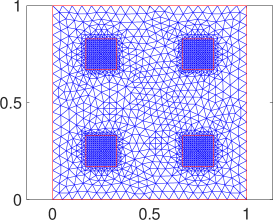
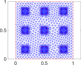
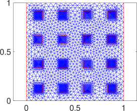
Figure 2. Actuators locations and triangulations of $\Omega$

The remainder of this section is split into two parts. The first one aims to confirm the statement of the stabilization result in Corollary 3.11. For this purpose we consider feedback controls of the form $\mathcal{K}^{\lambda}_{M}({P}_{\mathcal{U}_{M}}y)=-\lambda P_{\mathcal{U}_{M}}y$, $\lambda>0$, and show that the closed-loop system is exponentially stable in the $H$-norm provided the number $M_{\sigma}=\dim{\mathcal{U}}_{M}$ of actuators and the scalar $\lambda>0$ are both large enough. In the second part we compare $\mathcal{K}^{\lambda}_{M}({P}_{\mathcal{U}_{M}}y)$ with neural network induced feedback laws $\mathcal{K}^{(\theta)}_{M}({P}_{\mathcal{U}_{M}}y)$ obtained from solving the learning problem.

For the numerical approximation of (6.1) in space we rely on a piecewise linear finite element ansatz on locally refined triangulations of $\Omega$ which well resolve the support of the actuators. The meshes chosen for $4,~{}9,~{}16$ actuators are depicted in Figure 2. Concerning the temporal discretization, a semi-implicit time-stepping scheme with stepsize $k>0$ is applied. More precisely, the symmetric linear term $(-\nu\bigtriangleup+\mathbf{1}+a)y$ is treated by a Crank-Nicolson scheme and for the remaining terms a first order Adams-Bashforth method is used. All calculations were carried out in MATLAB.

6.1. Scaled orthogonal projection feedback laws

In the following we choose the following parameters in (1.13):

$$a\coloneqq-2+x_{1}-\left|\sin(t+x_{1})\right|_{{\mathbb{R}}}, \qquad b\coloneqq\begin{bmatrix}x_{1}+x_{2}\\ \cos(t)x_{1}x_{2}\end{bmatrix},\qquad y_{0}=\overline{y}_{0}\coloneqq\frac{1-2x_{1}x_{2}}{\left|1-2x_{1}x_{2}\right|_{H}},\quad\nu=0.1.$$

We briefly address the behavior of (6.1) if no control is applied i.e. for $\lambda=0$. In this case, the norm of the solution $y$ blows up in finite time, c.f. Figure 3. Note that the simulations were run for two different meshes namely those corresponding to $4$ and $16$ actuators, respectively. The computed results suggest that the blow-up time of the uncontrolled dynamics is independent of the spatial discretization.

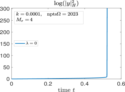
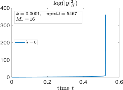
Figure 3. Free dynamics norm behavior.

Now we fix the number of actuators $M_{\sigma}=9$ and simulate (6.1) for varying values of $\lambda\geq 0$. The results are reported in Figure 4. Similar to the uncontrolled system, we observe a finite time blow-up of the solution norm for $\lambda=50,75,100$. Note that the blow-up time increases with $\lambda$. Finally, for $\lambda=125,150,175$, the system (6.1) is exponentially stable and the norm of $y$ is strictly decreasing. However we point out that the stabilization rate $\mu$ does not improve from $\lambda=150$ to $\lambda=175$. This backs up the claim of Corollary 3.11, which states that both $\lambda>0$ and $M\in\mathbb{N}$ have to be chosen large enough in order to achieve a certain rate of stabilization.

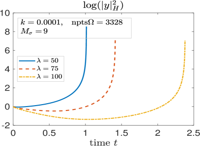
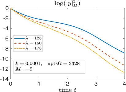
Figure 4. The case of $9$ actuators.

This becomes even more evident if we simulate (6.1) for the same values of $\lambda$ but with less/more actuators. In Figure 5 we see that $M_{\sigma}=4$ actuators are not able to stabilize the system, even for large $\lambda$. Moreover, the respective blow up times of for each $\lambda$ seem to convergence towards a limit point around $0.7$ as $\lambda$ increases. This behavior suggests that $4$ actuators are not able to stabilize the system independently of the value of $\lambda$. On the contrary with $M_{\sigma}=16$ actuators the system is stabilized for all considered values of $\lambda$. In particular note the improved rate of stabilization in comparison to the case of $M_{\sigma}=9$ in Figure 4.

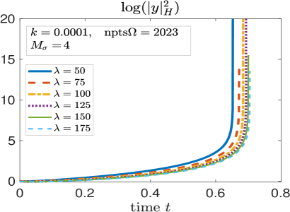
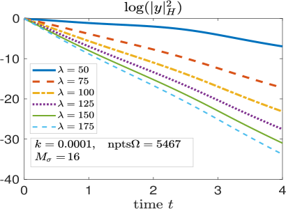
Figure 5. The case of $4$ and $16$ actuators.

Finally we repeat the previous simulations with $M_{\sigma}=16$ actuators for the rescaled initial condition $y_{0}=2\bar{y}_{0}$. The results can be found in Figure 6. After increasing the norm of the initial condition we note that $16$ actuators are no longer able to stabilize the system for $\lambda=50,75$. For the remaining larger values of $\lambda$, the system is still exponentially stable, however the rate of stabilization is smaller than in Figure 5.

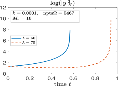
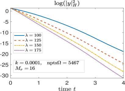
Figure 6. Larger initial condition, $y_{0}=2\overline{y}_{0}$.

In conclusion, Figures 3–6 backup the findings of Theorem 3.1. Indeed, they confirm the stabilizing property of the orthogonal projection feedback $\mathcal{K}^{\lambda}_{M}(P_{\mathcal{U}_{M}}y)=-\lambda P_{\mathcal{U}_{M}}y$ provided that both, the number of actuators $M_{\sigma}=\dim{\mathcal{U}}_{M}$ and the monotonicity parameter $\lambda>0$ are chosen large enough. Moreover Figure 6 shows that for larger initial conditions we (may) also need to increase $M_{\sigma}=\dim{\mathcal{U}}_{M}$ and/or $\lambda>0$ which highlights the semiglobal nature of the considered feedback.

As a last remark to this first part, note that we do not report here on simulations for the oblique projection feedback (c.f. Corollary 3.11), since its qualitative behavior parallels that of the orthogonal projection. For simulations concerning the linear case we refer the reader to [33].

6.2. Learning based feedback stabilization

Next we compare the orthogonal projection feedback $\mathcal{K}^{\lambda}_{M}(\mathcal{P}_{\mathcal{U}_{M}}\raisebox{-1.07639pt}{\scalebox{1.25}{$\cdot$}})$ for fixed $\lambda=100$ and $M_{\sigma}=9$ with neural network feedback laws $\mathcal{K}^{(\theta)}_{M}(\mathcal{P}_{\mathcal{U}_{M}}\raisebox{-1.07639pt}{\scalebox{1.25}{$\cdot$}})$ obtained from solving (4.4) with $\bar{\lambda}=100$. In this section the parameters in system (6.1) are chosen to be

$$a\coloneqq-2+x_{1}-\left|\sin(x_{1})\right|_{{\mathbb{R}}}, \qquad b\coloneqq\begin{bmatrix}x_{1}+x_{2}\\ x_{1}x_{2}\end{bmatrix},\qquad\nu=0.1,$$

and the initial state $y_{0}$ will be specified below. Moreover we denote by $\Delta_{h}$, $\nabla_{h}$ and $\mathcal{N}_{h}$ the finite element approximations of the diffusion and reaction operators as well as of the nonlinearity in (6.1). For the definitions and notation concerning neural networks used in the following we refer to Example 4.1. We choose feedback laws $\mathcal{K}^{(\theta)}_{M}$ induced by realizations $K^{(\theta)}_{M}$, c.f. (4.3), of neural networks $\theta$ with $L=3$ layers and architecture $\operatorname{arch}(\mathcal{R})=(9,15,15,9)$. The activation function is chosen as the softmax $\chi(x)=\log(1+\exp(x))$. Moreover we fix the finite time horizon $T=5$, the cost parameter $\beta=1$, the timestep $k=0.001$ and $\mathcal{G}(\theta)=0$. We point out that $T$, $L$ and $\operatorname{arch}(\mathcal{R})$ are chosen based on numerical experience. A systematic approach on how to choose the best neural network architecture for the stabilization problem at hand is beyond of the scope of this manuscript. Finally we address the choice of the “training set” in (4.4). For this purpose denote by $\lambda_{j}\in\mathbb{R}$ the eigenvalues of $(-\nu\Delta_{h}+\mathbf{1})$ ordered by increasing magnitude and let $v_{j}$ be the associated eigenfunctions. Now define the initial conditions $y^{i}_{0}$, $i=1,\dots,N_{0}$, $N_{0}=10$, in the training set by $y^{j}_{0}=v_{j}$ and $y^{j+5}_{0}=-v_{j}$, $j=1,\dots,5$. The learning grid $\{u_{i}\}^{N_{1}}_{i=1}$, $N_{1}=50000$, is obtained by uniformly sampling from the set

$$\mathbf{U}_{M}:=\left\{\,u\in L^{2}(\Omega)\;|\;u\in\mathcal{U}_{M},~{}|u|_{H}\leq 1.1\,\right\}.$$

The parameter $\varepsilon_{1}$ in the definition of $\mathcal{G}^{N_{1}}_{\gamma}$ is chosen as $\varepsilon_{1}=10^{-4}$. A gradient descent method is applied to all arising learning problems, that is, starting from $\theta_{0}\in\mathcal{R}$ we iterate $\theta_{k+1}=\theta_{k}-s_{k}\,\partial\mathcal{J}(\theta_{k})$ for some stepsize $s_{k}\geq 0$.

6.2.1. Computing neural network feedback laws

We now determine two neural network feedbacks, one for $\gamma=0$ (i.e., monotonicity is not enforced) and one for $\gamma=500$. We stress that, since the uncontrolled systems might blow-up in finite time, finding an initial neural network $\theta_{0}\in\mathcal{R}$ is not straightforward. As a remedy we consider the damped closed loop systems

$$\tfrac{\partial}{\partial t}y_{i}+(-0.1\Delta_{h}+{\mathbf{1}})y_{i}+ay_{i}+b\cdot\nabla_{h}y_{i}-\alpha\,\left|y_{i}\right|_{{\mathbb{R}}}y_{i}=\mathcal{K}^{(\theta)}_{M}(P_{{\mathcal{U}}_{M}}y_{i}),\quad\!\tfrac{\partial}{\partial{\mathbf{n}}}y_{i}\left.\kern-2.4pt\right|_{1\Gamma}=0,\quad\!y(0)=y^{i}_{0},$$ (6.2)

for $\alpha\in[0,1]$, $i=1,\dots,10$. For $\alpha=0$, the uncontrolled systems are linear and thus admit a solution on $[0,T]$. In virtue of the implicit function theorem, the same will be true for feedback laws $\mathcal{K}^{(\theta)}_{M}$ with small weights $\theta$. Now we can solve (4.4) subject to (6.2) and $\alpha=0$. Then path-following with respect to the damping parameter is carried out, by increasing $\alpha$ and solving(4.4) subjected to (6.2) using the previous solution as a starting point. This procedure is repeated until we arrive at $\alpha=1$. A similar homotopy strategy is applied for the penalty parameter, from $\gamma=0$ to $\gamma=500$.

Remark 6.1.

We observe that $\mathcal{K}^{(\theta_{0})}_{M}(P_{\mathcal{U}_{M}}\raisebox{-1.07639pt}{\scalebox{1.25}{$\cdot$}})=-\lambda P_{\mathcal{U}_{M}}$ for $\theta_{0}=(0,0,0,\cdots,0,-\lambda{\mathbf{1}},0)$. This observation might suggest to use the orthogonal projection feedback as a starting point for the learning problem. However, due to the definition of $K^{(\theta)}_{M}$ as a composition, we readily verify that $\partial_{W_{1,j}}J(\theta_{0})=0$, $\partial_{b_{j}}J(\theta_{0})=0$, $j=1,\dots,L$, as well as $\partial_{W_{2,j}}J(\theta_{0})=0$, $j=1,\dots,L-1$. Hence we have $\theta_{k}=(0,0,0,\cdots,0,W^{k}_{2,L},0)$ for some $W^{k}_{2,L}\in\mathbb{R}^{M_{\sigma}\times M_{\sigma}}$, that is, all realizations would result in linear mappings. Therefore we do not use this particular choice of $\theta_{0}$ as initialization for the algorithm.

6.2.2. Comparison for explicit initial conditions

To compare the neural network and orthogonal projection feedback laws we simulate the associated closed loop system for two initial conditions given by

$$\bar{y}^{1}_{0}\coloneqq\frac{1-2x_{1}x_{2}}{\left|1-2x_{1}x_{2}\right|_{H}},\qquad\bar{y}^{2}_{0}\coloneqq\frac{-\operatorname{sgn}(x_{1}-0.5)\,\operatorname{sgn}(x_{2}-0.5)}{\left|\operatorname{sgn}(x_{1}-0.5)\,\operatorname{sgn}(x_{2}-0.5)\right|_{H}}.$$

Note that these initial conditions are neither contained in the training set nor in its linear span. The temporal evolution of the $H$-norm of the computed states and feedback controls are plotted in Figures 7 and 8. Note the logarithmic scale, which is used for the vertical axis, and the additional zoomed plots showing the short-time behavior of the feedback controls.

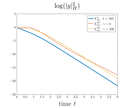
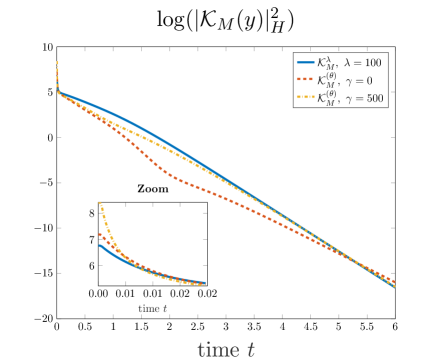
Figure 7. Evolution of state and control norms for $y_{0}=\bar{y}^{1}_{0}$.

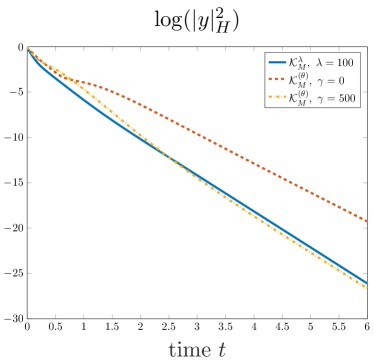
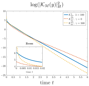
Figure 8. Evolution of state and control norms for $\bar{y}^{2}_{0}$.

Initial condition $\bar{y}^{1}_{0}$
$\qquad\mathcal{K}_{M}$		$|y|^{2}_{L^{2}}$	$|u|^{2}_{L^{2}}$	$J(y,u)$
$\mathcal{K}^{\lambda}_{M}$, $\lambda=100$		0.38	69.86	35.12
$\mathcal{K}^{(\theta)}_{M}$, $\gamma=0$		1.08	44.86	22.97
$\mathcal{K}^{(\theta)}_{M}$, $\gamma=500$		0.84	50.3	25.57

Initial condition $\bar{y}^{2}_{0}$
$\qquad\mathcal{K}_{M}$		$|y|^{2}_{L^{2}}$	$|u|^{2}_{L^{2}}$	$J(y,u)$
$\mathcal{K}^{\lambda}_{M}$, $\lambda=100$		0.11	17.06	8.57
$\mathcal{K}^{(\theta)}_{M}$, $\gamma=0$		0.18	10.34	5.26
$\mathcal{K}^{(\theta)}_{M}$, $\gamma=500$		0.16	13.08	6.62

Table 1. Results for $y_{0}\in\{\bar{y}^{1}_{0},\bar{y}^{2}_{0}\}$.

In Table 1 the values of objective functional as well as the space-time norms of the state trajectories, and the controls associated to the various feedback laws are summarized. In both examples all considered feedbacks eventually stabilize the system at (approximately) the same exponential rate. Additionally we observe that, in each example, the long-term behavior of the feedback controls is similar. However, the results significantly differ in the early stages. First we focus on the case $y_{0}=\bar{y}^{1}_{0}$. As expected, for both, the orthogonal projection and the neural network feedback with $\gamma=500$, the $H$-norm of $y$ is a strictly decreasing function. Note the slightly worse rate of stabilization for $\mathcal{K}^{(\theta)}_{M}$, $\gamma=500$, in the transient phase. In contrast, the norm of the state associated to $\mathcal{K}^{(\theta)}_{M}$, $\gamma=0$, increases on $[0,1]$. These observations are also reflected in slightly larger space-time norms of the state trajectories of the neural network controlled systems as we can see in Table 1, where $L^{2}$ stands for $L^{2}((0,T),L^{2}(\Omega))$. On the other hand we note that, apart from a short early phase, the neural network feedback controls are smaller than the ones induced by the orthogonal projection, resulting in significantly smaller control costs. As a consequence, the neural network induced feedback law $\mathcal{K}^{(\theta)}_{M}$, $\gamma=0$, admits the lowest overall objective functional value among all considered feedback laws followed by $\mathcal{K}^{(\theta)}_{M}$, $\gamma=500$, with an improvement of $35\%$ and $27\%$, respectively, over the explicit feedback.

We also make the same qualitative and quantitative observations for the case $y_{0}=\bar{y}^{2}_{0}$. Indeed, the state and control norms for the various feedbacks show comparable long-time behavior, but they differ in the early stages. This leads to slightly increased space-time state norms for the neural network feedback laws at the advantage of significantly reduced control costs. Overall this results in $39\%$, for $\gamma=0$, and $23\%$, for $\gamma=500$, smaller objective functional values for the neural network feedback laws in comparison to the scaled orthogonal projection based feedback law.

6.2.3. Validation for a large set of initial conditions

Finally we repeat the previous simulations for a larger number of randomly generated initial conditions to highlight the semiglobal nature of the considered feedback laws. For this purpose we uniformly sample functions $y^{j}_{0}$, $j=1,\dots,100$, from the validation set

$$\mathbf{Y}_{m}:=\left\{\,y_{0}\in H\;|\;y_{0}\in\operatorname{span}\{v_{j}\}^{m}_{j=1},~{}|y_{0}|_{H}\leq 1\,\right\}$$

where $m\in\mathbb{N}$ and $v_{j}$, $j=1,\dots,m$, denote the eigenfunctions from Section 6.2.2. Note that for $m\leq 5$, $\mathbf{Y}_{m}$ is a subset of the linear span of the training set. For each considered feedback law $\mathcal{K}_{M}$ and initial condition $y^{i}_{0}$ we then compute the associated states $y_{i}$ and feedback controls $u_{i}\coloneqq\mathcal{K}_{M}(P_{\mathcal{U}_{M}}y_{i})$. The indices of all initial conditions which are successfully stabilized are collected in the set

$$\mathcal{I}(\mathcal{K}_{M}):=\left\{\,i\in\{1,\dots,100\}\;|\;J(y_{i},u_{i})<\infty\,\right\}.$$

Moreover we define the numbers of failed and successful stabilizations by $\text{N}_{\text{succ}}\coloneqq\#\mathcal{I}(\mathcal{K}_{M})$ and $\text{N}_{\text{fail}}\coloneqq 100-\text{N}_{\text{succ}}$, respectively, as well as the averaged state/control norms and objective functional values:

$$\mathbb{E}\left[|y|^{2}_{L^{2}}\right]\coloneqq\frac{1}{\text{N}_{\text{succ}}}\sum_{i\in\mathcal{I}(\mathcal{K}_{M})}|y_{i}|^{2}_{L^{2}},~{}\mathbb{E}\left[|u|^{2}_{L^{2}}\right]\coloneqq\frac{1}{\text{N}_{\text{succ}}}\sum_{i\in\mathcal{I}(\mathcal{K}_{M})}|u_{i}|^{2}_{L^{2}},~{}\mathbb{E}\left[J(y,u)\right]\coloneqq\frac{1}{\text{N}_{\text{succ}}}\sum_{i\in\mathcal{I}(\mathcal{K}_{M})}J(y_{i},u_{i}).$$

Further $\text{N}_{\text{improv}}$ is the number of initial conditions for which $\mathcal{K}^{\theta}_{M}$ successfully stabilizes and the value of the objective functional is small than for the $\mathcal{K}^{\lambda}_{M}$ feedback law. In order to assess the performance of the various neural network feedback laws in comparison to the orthogonal projection we also compute the average as well as the best and worst improvement of the objective functional values

$$\text{Avg. Improv.}\coloneqq\left(\sum_{i\in\mathcal{I}(\mathcal{K}_{M})}\left(J(y_{i},u_{i})-J(y^{\lambda}_{i},u^{\lambda}_{i})\right)\right)/\sum_{i\in\mathcal{I}(\mathcal{K}_{M})}J(y^{\lambda}_{i},u^{\lambda}_{i}),$$

$$\text{Best}\coloneqq- \max_{i\in\mathcal{I}(\mathcal{K}_{M})}\left\{\frac{J(y^{\lambda}_{i},u^{\lambda}_{i})-J(y_{i},u_{i})}{J(y^{\lambda}_{i},u^{\lambda}_{i})}\right\}\ ,~{}\text{Worst}\coloneqq-\min_{i\in\mathcal{I}(\mathcal{K}_{M})}\left\{\frac{J(y^{\lambda}_{i},u^{\lambda}_{i})-J(y_{i},u_{i})}{J(y^{\lambda}_{i},u^{\lambda}_{i})}\right\}$$

where $y^{\lambda}_{i}$ and $u^{\lambda}_{i}$ denote the state and feedback controls associated to $\mathcal{K}^{\lambda}_{M}$. The computed results for $m=5,7,10$ can be found in Table 2 and 3, respectively.

$\qquad\mathcal{K}_{M}$		$\text{N}_{\text{fail}}$	$\text{N}_{\text{improv}}$	$\mathbb{E}\left[|y|^{2}_{L^{2}}\right]$	$\mathbb{E}\left[|u|^{2}_{L^{2}}\right]$	$\mathbb{E}\left[J(y,u)\right]$	Avg. Improv.	Best	Worst
$\mathcal{K}^{\lambda}_{M}$, $\lambda=100$		0	0	0.07	12.6	6.35	$+0\%$	$+0\%$	$+0\%$
$\mathcal{K}^{(\theta)}_{M}$, $\gamma=0$		2	98	0.2	6.3	3.24	$-44\%$	$-96\%$	$-6\%$
$\mathcal{K}^{(\theta)}_{M}$, $\gamma=500$		0	82	0.1	10.1	5.12	$-19\%$	$-86\%$	$+46\%$

Table 2. Validation results for $m=5$.

$\qquad\mathcal{K}_{M}$		$\text{N}_{\text{fail}}$	$\text{N}_{\text{improv}}$	$\mathbb{E}\left[|y|^{2}_{L^{2}}\right]$	$\mathbb{E}\left[|u|^{2}_{L^{2}}\right]$	$\mathbb{E}\left[J(y,u)\right]$	Avg. Improv.	Best	Worst
$\mathcal{K}^{\lambda}_{M}$, $\lambda=100$		0	0	0.06	10.6	5.34	$+0\%$	$+0\%$	$+0\%$
$\mathcal{K}^{(\theta)}_{M}$, $\gamma=0$		2	98	0.15	4.6	2.37	$-50\%$	$-95\%$	$-12\%$
$\mathcal{K}^{(\theta)}_{M}$, $\gamma=500$		0	53	0.08	10	5.04	$-6\%$	$-72\%$	$+67\%$

Table 3. Validation results for $m=7$.

$\qquad\mathcal{K}_{M}$		$\text{N}_{\text{fail}}$	$\text{N}_{\text{improv}}$	$\mathbb{E}\left[|y|^{2}_{L^{2}}\right]$	$\mathbb{E}\left[|u|^{2}_{L^{2}}\right]$	$\mathbb{E}\left[J(y,u)\right]$	Avg. Improv.	Best	Worst
$\mathcal{K}^{\lambda}_{M}$, $\lambda=100$		0	0	0.05	8.3	4.18	$+0\%$	$+0\%$	$+0\%$
$\mathcal{K}^{(\theta)}_{M}$, $\gamma=0$		1	99	0.11	3.7	1.9	$-50\%$	$-94\%$	$-12\%$
$\mathcal{K}^{(\theta)}_{M}$, $\gamma=500$		0	16	0.06	10.3	5.12	$+23\%$	$-36\%$	$+164\%$

Table 4. Validation results for $m=10$.

As a starting point for the discussion of these results, note that the orthogonal projection $\mathcal{K}^{\lambda}_{M}$ and the monotone neural network feedback $\mathcal{K}^{(\theta)}_{M}$, $\gamma=500$, stabilize all sampled initial conditions. In contrast, $\mathcal{K}^{(\theta)}_{M}$, $\gamma=0$, which is learned without the monotony enhancing penalty term fails in a small percentage of cases. From a quantitative perspective, we make similar observations as for the explicit initial conditions in the previous section. Let us first focus on $\mathcal{K}^{(\theta)}_{M}$, $\gamma=0$. In all tests we have $\text{N}_{\text{succ}}=\text{N}_{\text{improv}}$. Thus, if $\mathcal{K}^{(\theta)}_{M}$ successfully stabilizes one of the sampled initial condition, it admits a smaller objective functional value than $\mathcal{K}^{\lambda}_{M}$ with an average improvement of about $50\%$. As in Section 6.2.2, this traces back to a significant decrease in the norm of the feedback controls. Finally the results indicate that the improvement of the neural network feedback law for $\gamma=0$ is independent of $m\in\mathbb{N}$. This suggests that while we are learning the feedback on a relatively small set of $10$ initial conditions it successfully generalizes to functions outside of the training set without losing its stabilizing properties and without a loss of performance.

The behavior of the neural network feedback learned with the monotony enhancing penalty term differs in certain key aspects. For example, while $\mathcal{K}^{(\theta)}_{M}$, $\gamma=500$, stabilizes in all considered test cases, that is, $\text{N}_{\text{succ}}=100$, it does not always improve over the orthogonal projection and thus $\text{N}_{\text{improv}}<100$. Additionally its performance in comparison to $\mathcal{K}^{\lambda}_{M}$ deteriorates for growing $m\in\mathbb{N}$. Indeed, while we observe smaller objective function values for $\text{N}_{\text{improv}}=86$ initial conditions with an average improvement of $-20\%$ over $\mathcal{K}^{\lambda}_{M}$ for $m=5$, this decreases to $\text{N}_{\text{improv}}=53$ at $-6\%$ for $m=7$. Finally, for $m=10$, the neural network feedback only improves in $\text{N}_{\text{improv}}=16$ cases and, on average, performs worse than the orthogonal projection feedback. To explain this loss of performance we point out that the average state and controls norms as well as the averaged objective functional values associated to $\mathcal{K}^{\lambda}_{M}$ become smaller as $m\in\mathbb{N}$ grows. The same holds true for $\mathcal{K}^{(\theta)}_{M}$, $\gamma=0$. In contrast, the monotone neural network feedback law fails to adapt this improved behavior on the larger validation sets, that is, the average control cost and the objective functional value is independent of $m\in\mathbb{N}$. Thus it generalizes worse than the other feedbacks to initial conditions outside of the training set.

In summary, on the one hand, the results of this section show the great potential and success of learning feedback laws for the stabilization of unstable, nonlinear, parabolic systems. On the other hand, they also point out certain limitations of this approach which stimulate further research. For example, the performance of the neural network feedback law learned without the penalty term could be further improved by adaptively enlarging the training set with those initial conditions from $\mathbf{Y}_{m}$ for which $\mathcal{K}^{(\theta)}_{M}$ fails. Moreover, the discussion in the last paragraph suggests that the performance of the monotone neural network feedback law is more susceptible to the choice of the training set. Clearly, this raises the question on how to choose the initial conditions for the training of the network in an optimal way as wells as on the robustness of the computed results with respect to changes in the training set.

Appendix

A.3. Proof of Lemma 3.5

Using Lemma 3.3 with $(y_{1},y_{2})=(y,0)$, we find

$$2({\mathcal{N}}(y),Ay)_{H} \leq\gamma_{2}\left|y\right|_{{\mathrm{D}}(A)}^{2}+D_{1}\sum\limits_{j=1}^{n}\left|y\right|_{{\mathrm{D}}(A)}^{\frac{2\zeta_{2j}}{1-\delta_{2j}}}\left|y\right|_{V}^{\frac{2\zeta_{1j}+2\delta_{1j}}{1-\delta_{2j}}},\quad\mbox{for all}\quad\gamma_{2}>0,$$ (A.1)

with $D_{1}\coloneqq\left(1+\gamma_{2}^{-\frac{1+\|\delta_{2}\|}{1-\|\delta_{2}\|}}\right)\overline{C}_{{\mathcal{N}}1}$. Next, we recall the young inequality in the form

$$ab\leq\tfrac{1}{s}\eta^{s}a^{s}+\tfrac{s-1}{s}\eta^{-\frac{s}{s-1}}a^{\frac{s}{s-1}},\quad\mbox{for all}\quad a\geq 0,\;b\geq 0,\;\eta>0,\;s>1,$$

(cf. [31, Appendix A.1]), which allow us to obtain, with

$$s=s_{j}=\tfrac{1-\delta_{2j}}{\zeta_{2j}}>1,\qquad\tfrac{s_{j}-1}{s_{j}}=\tfrac{1-\delta_{2j}-\zeta_{2j}}{1-\delta_{2j}},\qquad\mbox{in case}\quad\zeta_{2j}>0,$$

the inequality

$$\left|y\right|_{{\mathrm{D}}(A)}^{\frac{2\zeta_{2j}}{1-\delta_{2j}}}\left|y\right|_{V}^{\frac{2\zeta_{1j}+2\delta_{1j}}{1-\delta_{2j}}} \leq\tfrac{\zeta_{2j}}{1-\delta_{2j}}\eta_{j}^{\frac{1-\delta_{2j}}{\zeta_{2j}}}\left|y\right|_{{\mathrm{D}}(A)}^{2}+\tfrac{1-\delta_{2j}-\zeta_{2j}}{1-\delta_{2j}}\eta_{j}^{-\frac{1-\delta_{2j}}{1-\delta_{2j}-\zeta_{2j}}}\left|y\right|_{V}^{\frac{2\zeta_{1j}+2\delta_{1j}}{1-\delta_{2j}-\zeta_{2j}}},\quad\mbox{for all}\quad\eta_{j}>0.$$

Now, for any given $\gamma_{3}>0$, we choose

$$\eta_{j}=(\tfrac{1-\delta_{2j}}{\zeta_{2j}}\gamma_{3})^{\frac{\zeta_{2j}}{1-\delta_{2j}}},\quad\mbox{in case}\quad\zeta_{2j}>0.$$

which gives us

$$\left|y\right|_{{\mathrm{D}}(A)}^{\frac{2\zeta_{2j}}{1-\delta_{2j}}}\left|y\right|_{V}^{\frac{2\zeta_{1j}+2\delta_{1j}}{1-\delta_{2j}}} \leq\gamma_{3}\left|y\right|_{{\mathrm{D}}(A)}^{2}+\tfrac{1-\delta_{2j}-\zeta_{2j}}{1-\delta_{2j}}(\tfrac{1-\delta_{2j}}{\zeta_{2j}}\gamma_{3})^{-\frac{\zeta_{2j}}{1-\delta_{2j}-\zeta_{2j}}}\left|y\right|_{V}^{\frac{2\zeta_{1j}+2\delta_{1j}}{1-\delta_{2j}-\zeta_{2j}}},\quad\mbox{in case}\quad\zeta_{2j}>0.$$

Recalling (A.1), it follows that

$$2({\mathcal{N}}(y),Ay)_{H} \leq\gamma_{2}\left|y\right|_{{\mathrm{D}}(A)}^{2}+D_{1}\sum\limits_{\begin{subarray}{c}1\leq j\leq n\\ \zeta_{2j}=0\end{subarray}}\left|y\right|_{V}^{\frac{2\zeta_{1j}+2\delta_{1j}}{1-\delta_{2j}}}+D_{1}\sum\limits_{\begin{subarray}{c}1\leq j\leq n\\ \zeta_{2j}>0\end{subarray}}\left(\gamma_{3}\left|y\right|_{{\mathrm{D}}(A)}^{2}+D_{2}\left|y\right|_{V}^{\frac{2\zeta_{1j}+2\delta_{1j}}{1-\delta_{2j}-\zeta_{2j}}}\right)$$

$$\leq(\gamma_{2}+D_{1}\gamma_{3}n)\left|y\right|_{{\mathrm{D}}(A)}^{2}+D_{1}(1+D_{2})\sum\limits_{j=1}^{n}\left|y\right|_{V}^{\frac{2\zeta_{1j}+2\delta_{1j}}{1-\delta_{2j}-\zeta_{2j}}},$$ (A.2a)

for all $$\gamma_{2}>0 \gamma_{3}>0$$, , with

$$D_{2} =\max_{\begin{subarray}{c}1\leq j\leq n\\ \zeta_{2j}\neq 0\end{subarray}}\tfrac{1-\delta_{2j}-\zeta_{2j}}{1-\delta_{2j}}(\tfrac{1-\delta_{2j}}{\zeta_{2j}}\gamma_{3})^{-\frac{\zeta_{2j}}{1-\delta_{2j}-\zeta_{2j}}}.$$ (A.2b)

Now for an arbitrary given $\gamma_{4}>0$, we may set $\gamma_{2}=\frac{\gamma_{4}}{2}$ and $\gamma_{3}=\frac{\gamma_{4}}{2nD_{1}}$, leading us to

$$2({\mathcal{N}}(y),Ay)_{H}\leq\gamma_{4}\left|y\right|_{{\mathrm{D}}(A)}^{2}+D_{1}(1+D_{2})\sum\limits_{j=1}^{n}\left|y\right|_{V}^{\frac{2\zeta_{1j}+2\delta_{1j}}{1-\delta_{2j}-\zeta_{2j}}},\quad\mbox{for all}\quad\gamma_{4}>0.$$ (A.3)

Observe that

$$\tfrac{2\zeta_{1j}+2\delta_{1j}}{1-\delta_{2j}-\zeta_{2j}}\geq 2 \quad\Longleftrightarrow\quad\zeta_{1j}+\delta_{1j}\geq 1-\delta_{2j}-\zeta_{2j}\quad\Longleftrightarrow\quad\delta_{2j}+\delta_{1j}-1\geq-\zeta_{1j}-\zeta_{2j},$$

hence, from Assumption 2.4, we have that

$$p_{j}\coloneqq 2-\tfrac{2\zeta_{1j}+2\delta_{1j}}{1-\delta_{2j}-\zeta_{2j}}\geq 0$$

and can write

$$2({\mathcal{N}}(y),Ay)_{H} \leq\gamma_{4}\left|y\right|_{{\mathrm{D}}(A)}^{2}+D_{1}(1+D_{2})\left|y\right|_{V}^{2}\sum\limits_{j=1}^{n}\left|y\right|_{V}^{p_{j}}$$

$$\leq\gamma_{4}\left|y\right|_{{\mathrm{D}}(A)}^{2}+nD_{1}(1+D_{2})\left|y\right|_{V}^{2}(1+\left|y\right|_{V}^{\|p\|})\quad\mbox{for all}\quad\gamma_{4}>0,$$

with

$$\|p\| =\max_{1\leq j\leq n}p_{j},\qquad D_{1}=\left(1+(\tfrac{\gamma_{4}}{2})^{-\frac{1+\|\delta_{2}\|}{1-\|\delta_{2}\|}}\right)\overline{C}_{{\mathcal{N}}1},$$

$$\quad\mbox{and}\quad D_{2} =\max_{\begin{subarray}{c}1\leq j\leq n\\ \zeta_{2j}\neq 0\end{subarray}}\tfrac{1-\delta_{2j}-\zeta_{2j}}{1-\delta_{2j}}(\tfrac{1-\delta_{2j}}{\zeta_{2j}}\tfrac{\gamma_{4}}{2nD_{1}})^{-\frac{\zeta_{2j}}{1-\delta_{2j}-\zeta_{2j}}}.$$

This ends the proof.∎

Acknowledgements.

Karl Kunisch and Sérgio Rodrigues were supported in part by the ERC advanced grant 668998 (OCLOC) under the EU’s H2020 research program. Sérgio Rodrigues also acknowledges partial support from Austrian Science Fund (FWF): P 33432-NBL.

References

• [1] B. Azmi and S. S. Rodrigues. Oblique projection local feedback stabilization of nonautonomous semilinear damped wave-like equations. J. Differential Equations, 269(7):6163–6192, 2020. doi:10.1016/j.jde.2020.04.033.
• [2] A. Azouani and E. S. Titi. Feedback control of nonlinear dissipative systems by finite determining parameters – a reaction-diffusion paradigm. Evol. Equ. Control Theory, 3(4):579–594, 2014. doi:10.3934/eect.2014.3.579.
• [3] M. Badra and T. Takahashi. Stabilization of parabolic nonlinear systems with finite dimensional feedback or dynamical controllers: Application to the Navier–Stokes system. SIAM J. Control Optim., 49(2):420–463, 2011. doi:10.1137/090778146.
• [4] J. M. Ball. Remarks on blow-up and nonexistence theorems for nonlinear evolution equations. Q. J. Math., 28(4):473–486, 1977. doi:10.1093/qmath/28.4.473.
• [5] A. Balogh and M. Krstic. Burgers’ equation with nonlinear boundary feedback: $h^{1}$ stability, well-posedness and simulation. Math. Probl. Engineering, 6:189–200, 2000. doi:10.1155/S1024123X00001320.
• [6] V. Barbu. Stabilization of Navier–Stokes equations by oblique boundary feedback controllers. SIAM J. Control Optim., 50(4):2288–2307, 2012. doi:10.1137/110837164.
• [7] V. Barbu. Boundary stabilization of equilibrium solutions to parabolic equations. IEEE Trans. Automat. Control, 58(9):2416–2420, 2013. doi:10.1109/TAC.2013.2254013.
• [8] V. Barbu, I. Lasiecka, and R. Triggiani. Abstract settings for tangential boundary stabilization of Navier–Stokes equations by high- and low-gain feedback controllers. Nonlinear Anal., 64(12):2704–2746, 2006. doi:10.1016/j.na.2005.09.012.
• [9] V. Barbu, S. S. Rodrigues, and A. Shirikyan. Internal exponential stabilization to a nonstationary solution for 3D Navier–Stokes equations. SIAM J. Control Optim., 49(4):1454–1478, 2011. doi:10.1137/100785739.
• [10] V. Barbu and R. Triggiani. Internal stabilization of Navier–Stokes equations with finite-dimensional controllers. Indiana Univ. Math. J., 53(5):1443–1494, 2004. doi:10.1512/iumj.2004.53.2445.
• [11] D. P. Bertsekas. Reinforcement Learning and Optimal Control. Athena Scientific, Belmont, Massachusetts, 2019.
• [12] J. Cochran, R. Vazquez, and M. Krstic. Backstepping boundary control of Navier–Stokes channel flow: A 3D extension. In Proceedings of the 2006 American Control Conference, Minneapolis, Minnesota, USA, pages 769–774, 6 2006. URL: 10.1109/ACC.2006.1655449.
• [13] F. Demengel and G. Demengel. Functional Spaces for the Theory of Elliptic Partial Differential Equations. Universitext. Springer, 2012. doi:10.1007/978-1-4471-2807-6.
• [14] Sergey Dolgov, Dante Kalise, and Karl Kunisch. Tensor decompositions for high-dimensional hamilton-jacobi-bellman equations, 2019. arXiv:1908.01533.
• [15] W. E. Dynamics of vortex liquids in ginzburg-landau theories with applications to superconductivity. Phys. Rev. B, 50:1126–1135, 1994. doi:10.1103/PhysRevB.50.1126.
• [16] R. A. Fisher. The wave of advance of advantageous genes. Ann. Human Genetics, 7(4):355–369, 1937. doi:10.1111/j.1469-1809.1937.tb02153.x.
• [17] S. Grishakov, P.N. Degtyarenko, N.N. Degtyarenko, V.F. Elesin, and V.S. Kruglov. Time dependent Ginzburg–Landau equations for modeling vortices dynamics in type-II superconductors with defects under a transport current. Physics Procedia, 36:1206–1210, 2012. doi:10.1016/j.phpro.2012.06.202.
• [18] M. Gugat and F. Troeltzsch. Boundary feedback stabilization of the schlögl system. Automatica J. IFAC, 51:192–1199, 2015. doi:10.1016/j.automatica.2014.10.106.
• [19] A. Halanay, C. M. Murea, and C. A. Safta. Numerical experiment for stabilization of the heat equation by Dirichlet boundary control. Numer. Funct. Anal. Optim., 34(12):1317–1327, 2013. doi:10.1080/01630563.2013.808210.
• [20] M. Krstic, L. Magnis, and R. Vazquez. Nonlinear control of the viscous Burgers equation: Trajectory generation, tracking, and observer design. J. Dyn. Syst. Meas. Control, 131(2):021012(1–8), 2009. doi:10.1115/1.3023128.
• [21] K. Kunisch and S. S. Rodrigues. Explicit exponential stabilization of nonautonomous linear parabolic-like systems by a finite number of internal actuators. ESAIM Control Optim. Calc. Var., 25, 2019. Art 67. doi:10.1051/cocv/2018054.
• [22] K. Kunisch and S. S. Rodrigues. Oblique projection based stabilizing feedback for nonautonomous coupled parabolic-ode systems. Discrete Contin. Dyn. Syst., 39(11):6355–6389, 2019. doi:10.3934/dcds.2019276.
• [23] K. Kunisch and D. Walter. Semiglobal optimal feedback stabilization of autonomous systems via deep neural network approximation. Arxiv:2002.08625v1[math.OC], 2020. (submitted). URL: https://arxiv.org/abs/2002.08625.
• [24] D. Le. Global existence for some cross diffusion systems with equal cross diffusion/reaction rates. Adv. Nonlinear Stud. (pub. online), 2020. doi:10.1515/ans-2020-2096.
• [25] H. A. Levine. Some nonexistence and instability theorems for solutions of formally parabolic equations of the form ${P}u_{t}=-{A}u+{\mathcal{F}}(u)$. Arch. Ration. Mech. Anal., 51(5):371–386, 1973. doi:10.1007/BF00263041.
• [26] E. Lunasin and E. S. Titi. Finite determining parameters feedback control for distributed nonlinear dissipative systems – a computational study. Evol. Equ. Control Theory, 6(4):535–557, 2017. doi:10.3934/eect.2017027.
• [27] F. Merle and H. Zaag. Optimal estimates for blowup rate and behavior for nonlinear heat equations. Comm. Pure Appl. Math., 51(2):139–196, 1998. doi:10.1002/(SICI)1097-0312(199802)51:2<139::AID-CPA2>3.0.CO;2-C.
• [28] D. Olmos and B. D. Shizgal. A pseudospectral method of solution of Fisher’s equation. Journal of Computational and Applied Mathematics, 193(1):219–242, 2006. doi:10.1016/j.cam.2005.06.028.
• [29] D. Phan and S. S. Rodrigues. Stabilization to trajectories for parabolic equations. Math. Control Signals Syst., 30(2), 2018. Art 11. doi:10.1007/s00498-018-0218-0.
• [30] J.-P. Raymond. Stabilizability of infinite-dimensional systems by finite-dimensional controls. Comput. Methods Appl. Math., 19(4):797–811, 2019. doi:10.1515/cmam-2018-0031.
• [31] S. S. Rodrigues. Semiglobal exponential stabilization of nonautonomous semilinear parabolic-like systems. Evol. Equ. Control Theory, 9(3):635–672, 2020. doi:10.3934/eect.2020027.
• [32] S. S. Rodrigues. Oblique projection exponential dynamical observer for nonautonomous linear parabolic-like equations. SIAM J. Control Optim., 59(1):464–488, 2021. doi:10.1137/19M1278934.
• [33] S. S. Rodrigues. Oblique projection output-based feedback stabilization of nonautonomous parabolic equations. Automatica J. IFAC (accepted), 2021. RICAM Report No. 2020-33. URL: https://www.ricam.oeaw.ac.at/publications/ricam-reports/.
• [34] F. Schlögl. Chemical reaction models for non-equilibrium phase transitions. Z. Physik, 253:147–161, 1972. doi:10.1007/BF01379769.
• [35] N. Shigesada, K. Kawasaki, and E. Teramoto. Spatial segregation of interacting species. J. Theor. Biol., 79(1):83–99, 1979. doi:10.1016/0022-5193(79)90258-3.
• [36] D. Tsubakino, M. Krstic, and Sh. Hara. Backstepping control for parabolic PDEs with in-domain actuation. In Proceedings of the American Control Conference (ACC), Montréal, Canada, pages 2226–2231, 2012. doi:10.1109/ACC.2012.6315358.
• [37] M.Y. Wu. A note on stability of linear time-varying systems. IEEE Trans. Automat. Control, 19(2):162, 1974. doi:10.1109/TAC.1974.1100529.