Semi-Decentralized Federated Learning with Cooperative D2D Local Model Aggregations

Abstract

Federated learning has emerged as a popular technique for distributing machine learning (ML) model training across the wireless edge. In this paper, we propose two timescale hybrid federated learning (TT-HF), a semi-decentralized learning architecture that combines the conventional device-to-server communication paradigm for federated learning with device-to-device (D2D) communications for model training. In TT-HF, during each global aggregation interval, devices (i) perform multiple stochastic gradient descent iterations on their individual datasets, and (ii) aperiodically engage in consensus procedure of their model parameters through cooperative, distributed D2D communications within local clusters. With a new general definition of gradient diversity, we formally study the convergence behavior of TT-HF, resulting in new convergence bounds for distributed ML. We leverage our convergence bounds to develop an adaptive control algorithm that tunes the step size, D2D communication rounds, and global aggregation period of TT-HF over time to target a sublinear convergence rate of $\mathcal{O}(1/t)$ while minimizing network resource utilization. Our subsequent experiments demonstrate that TT-HF significantly outperforms the current art in federated learning in terms of model accuracy and/or network energy consumption in different scenarios where local device datasets exhibit statistical heterogeneity. Finally, our numerical evaluations demonstrate robustness against outages caused by fading channels, as well favorable performance with non-convex loss functions.

I Introduction

Machine learning (ML) techniques have exhibited widespread successes in applications ranging from computer vision to natural language processing [2, 3, 4]. Traditionally, ML model training has been conducted in a centralized manner, e.g., at datacenters, where the computational infrastructure and dataset required for training coexist. In many applications, however, the data required for model training is generated at devices which are distributed across the edge of communications networks. As the amount of data on each device increases, uplink transmission of local datasets to a main server becomes bandwidth-intensive and time consuming, which is prohibitive in latency-sensitive applications [5]. Common examples include object detection for autonomous vehicles [6] and keyboard next-word prediction on smartphones [7], each requiring rapid analysis of data generated from embedded sensors. Also, in many applications, end users may not be willing to share their datasets with a server due to privacy concerns [8].

I-A Federated Learning at the Wireless Edge

Federated learning has emerged as a popular distributed ML technique for addressing these bandwidth and privacy challenges [9, 10, 11]. A schematic of its conventional architecture is given in Fig. 1: in each iteration, each device trains a local model based on its own dataset, often using (stochastic) gradient descent. The devices then upload their local models to the server, which aggregates them into a global model, often using a weighted average, and synchronizes the devices with this new model to initiate the next round of local training.

Although widespread deployment of federated learning is desired [12, 13], its conventional architecture in Fig. 1 poses challenges for the wireless edge: the devices comprising the Internet of Things (IoT) may exhibit significant heterogeneity in their computational resources (e.g., a high-powered drone compared to a low-powered smartphone) [14]; additionally, the devices may exhibit varying proximity to the server (e.g., varying distances from smartphones to the base station in a cell), which may cause significant energy consumption for upstream data transmission [15].

To mitigate the cost of uplink and downlink transmissions, local model training coupled with periodic but infrequent global aggregations has been proposed [16, 17, 14]. Yet, the local datasets may exhibit significant heterogeneity in their statistical distributions [18], resulting in learned models that may be biased towards local datasets, hence degrading the global model accuracy [16].

In this setting, motivated by the need to mitigate divergence across the local models, we study the problem of resource-efficient federated learning across heterogeneous local datasets at the wireless edge. A key technology that we incorporate into our approach is device-to-device (D2D) communications among edge devices, which is a localized version of peer-to-peer (P2P) among direct physical connections. D2D communications is being envisioned in fog computing and IoT systems through 5G wireless [5, 18, 19]; indeed, it is expected that 50% of all network connections will be machine-to-machine by 2023 [18]. Through D2D, we design a consensus mechanism to mitigate model divergence via low-power communications among nearby devices. We call our approach two timescale hybrid federated learning (TT-HF), since it (i) involves a hybrid between device-to-device and device-to-server communications, and (ii) incorporates two timescales for model training: iterations of stochastic gradient descent at individual devices, and rounds of cooperative D2D communications within clusters. By inducing consensus in the local models within a cluster of devices, TT-HF promises resource efficiency, as we will show both theoretically and by simulation, since only one device from the cluster needs to upload the cluster model to the server during global aggregation, as opposed to the conventional federated learning architecture, where most of the devices are required to upload their local models [9]. Specifically, during the local update interval in federated learning, devices can systematically share their model parameters with others in their neighborhood to form a distributed consensus among each cluster of edge devices. Then, at the end of each local training interval, assuming that each device’s model now reflects the consensus of its cluster, the main server can randomly sample just one device from each cluster for the global aggregation. We call our approach two timescale hybrid federated learning (TT-HF), since it (i) involves a hybrid between device-to-device and device-to-server communications, and (ii) incorporates two timescales for model training: iterations of gradient descent at individual devices, and rounds of cooperative D2D communications within clusters.

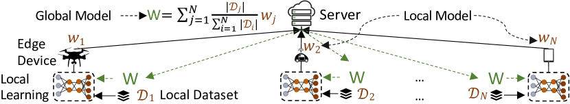
Figure 1: Conventional federated learning. In each training round, devices perform local model updates based on local datasets, followed by an aggregation at the main server to compute the global model, which is broadcast to the devices for the next round of local updates.

TT-HF migrates from the “star” topology of conventional federated learning in Fig. 1 to a semi-decentralized learning architecture, shown in Fig. 2, that includes local topologies between edge devices, as advocated in the new “fog learning” paradigm [18]. In doing so, we must carefully consider the relationships between device-level stochastic gradient updates, cluster-level consensus procedure, and network-level global aggregations. We quantify these relationships in this work, and use them to tune the lengths of each local update and consensus period. As we will see, the result is a version of federated learning which optimizes the global model convergence characteristics while minimizing the uplink communication requirement in the system.

I-B Related Work

A multitude of works on federated learning have emerged in the past few years, addressing various aspects, such as communication and computation constraints of wireless devices [20, 21, 15, 22], multi-task learning [23, 24, 25], and personalized model training [26, 27]. We refer the reader to e.g., [28, 29] for comprehensive surveys of the federated learning literature; in this section, we will focus on the works addressing resource efficiency, statistical data heterogeneity, and cooperative learning, which is the main focus of this paper.

In terms of wireless communication efficiency, several works have investigated the impact of performing multiple rounds of local gradient updates in-between consecutive global aggregations [30, 16], including optimizing the aggregation period according to a total resource budget [16]. To further reduce the demand for global aggregations, [31] proposed a hierarchical system model for federated learning where edge servers are utilized for partial global aggregations. Model quantization [32] and sparsification [33] techniques have also been proposed. As compared to above works, we propose a semi-decentralized architecture, where D2D communications are used to exchange model parameters among the nodes in conjunction with global aggregations. We show that our framework can reduce the frequency of global aggregations and result in network resource savings.

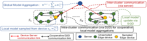
Figure 2: Network architecture of semi-decentralized federated learning. Edge devices form local cluster topologies based on their D2D communication capability. Cooperative local model aggregations among these clusters occur using D2D communications in between global aggregations conducted by the server.

Other works have considered improving model training in the presence of heterogeneous data among the devices via raw data sharing [34, 35, 14, 36]. In [34], the authors propose uploading portions of the local datasets to the server, which is then used to augment global model training. The works [36, 35, 14] mitigate local data heterogeneity by enabling the server to share a portion of its aggregated data among the devices [36], or by optimizing D2D data offloading [35, 14]. However, raw data sharing may suffer from privacy concerns or bandwidth limitations. In our framework, we exploit D2D communications to exchange model parameters among the devices, which alleviates such concerns.

Different from the above works, we propose a methodology that addresses the communication efficiency and data heterogeneity challenges simultaneously. To do this, we introduce distributed cooperative learning among devices into the local update process – as advocated recently [18] – resulting in a novel system architecture with D2D-augmented learning. In this regard, the most relevant work is [37], which also studies cluster-based consensus procedure between global aggregations in federated learning. Different from [37], we consider the case where (i) devices may conduct multiple (stochastic) gradient iterations between global aggregations, (ii) the global aggregations are aperiodic, and (iii) consensus procedure among the devices may occur aperiodically during each global aggregation. We further introduce a new metric of gradient diversity that extends the previous existing definition in literature. Doing so leads to a more complex system model, which we analyze to provide improvements to resource efficiency and model convergence. Consequently, the techniques used in the convergence analysis and the bound obtained differ significantly from [37]. There is also an emerging set of works on fully decentralized (server-less) federated learning [38, 39, 40, 41]. However, these architectures require a well-connected communication graph among all the devices in the network, which may not be scalable to large-scale systems where devices from various regions/countries are involved in ML model training. Our work can be seen as intermediate between the star topology assumed in conventional federated learning and fully decentralized architectures, and constitutes a novel semi-decentralized learning architecture that mitigates the cost of resource intensive uplink communications of conventional server-based methods over star topologies, achieved via local low-power D2D communications, while improving scalability over fully decentralized server-less architectures.

Finally, note that there is a well-developed literature on consensus-based optimization, e.g., [42, 43, 44, 45]. Our work employs the distributed average consensus technique and exploits that in a new semi-decentralized machine learning architecture and contributes new results on distributed ML to this literature.

I-C Outline and Summary of Contributions

• We propose two timescale hybrid federated learning (TT-HF), which augments the conventional federated learning architecture with aperiodic consensus procedure of models within local device clusters and aperiodic global aggregations by the server (Sec. II).

• We propose a new model of gradient diversity, and theoretically investigate the convergence behavior of TT-HF through techniques including coupled dynamic systems (Sec. III). Our bounds quantify how properties of the ML model, device datasets, consensus process, and global aggregations impact the convergence speed of TT-HF. In doing so, we obtain a set of conditions under which TT-HF converges at a rate of $\mathcal{O}(1/t)$, similar to centralized stochastic gradient descent.

• We develop an adaptive control algorithm for TT-HF that tunes the global aggregation intervals, the rounds of D2D performed by each cluster, and the learning rate over time to minimize a trade-off between energy consumption, delay, and model accuracy (Sec. IV). This control algorithm obtains the $\mathcal{O}(1/t)$ convergence rate by including our derived conditions as constraints in the optimization.

• Our subsequent experiments on popular learning tasks (Sec. V) verify that TT-HF outperforms federated learning with infrequent global aggregations, which is commonly used in literature, substantially in terms of resource consumption and/or training time over D2D-enabled wireless devices. They also confirm that the control algorithm is able to address resource limitations and data heterogeneity across devices by adapting the local and global aggregation periods.

We conclude in Sec. VI with some concluding remarks.

II System Model and Learning Methodology

In this section, we first describe our edge network system model of D2D-enabled clusters (Sec. II-A) and formalize the ML task for the system (Sec. II-B). Then, we develop our two timescale hybrid federated learning algorithm, TT-HF (Sec. II-C).

II-A Edge Network System Model

We consider model learning over the network architecture depicted in Fig. 2. The network consists of an edge server (e.g., at a base station) and $I$ edge devices gathered by the set $\mathcal{I}=\{1,\cdots,I\}$. We consider a cluster-based representation of the edge, where the devices are partitioned into $N$ sets $\mathcal{S}_{1},\cdots,\mathcal{S}_{N}$. Cluster $\mathcal{S}_{c}$ contains $s_{c}=|\mathcal{S}_{c}|$ edge devices, where $\sum_{c=1}^{N}s_{c}=I$. We assume that the clusters are formed based on the ability of devices to conduct low-energy D2D communications, e.g., geographic proximity. Thus, one cluster may be a fleet of drones while another is a collection of local IoT sensors. In general, we do not place any restrictions on the composition of devices within a cluster, as long as they possess a common D2D protocol [18] and communicate with a common server.

For edge device $i\in\mathcal{S}_{c}$, we let $\mathcal{N}_{i}\subseteq S_{c}$ denote the set of its D2D neighbors, determined based on the transmit power of the nodes, the channel conditions between them, and their physical distances (cluster topology is evaluated numerically in Sec. V based on a wireless communications model). We assume that D2D communications are bidirectional, i.e., $i\in\mathcal{N}_{i^{\prime}}$ if and only if ${i^{\prime}}\in{\mathcal{N}}_{i}$, $\forall i,i^{\prime}\in\mathcal{S}_{c}$. Based on this, we associate a network graph $G_{c}=(\mathcal{S}_{c},\mathcal{E}_{c})$ to each cluster, where $\mathcal{E}_{c}$ denotes the set of edges: $(i,{i^{\prime}})\in\mathcal{E}_{c}$ if and only if $i,i^{\prime}\in\mathcal{S}_{c}$ and $i\in\mathcal{N}_{i^{\prime}}$.

The model training is carried out through a sequence of global aggregations indexed by $k=1,2,\cdots$, as will be explained in Sec. II-C. Between global aggregations, the edge devices $i\in\mathcal{S}_{c}$ will participate in cooperative consensus procedure with their neighbors $i^{\prime}\in\mathcal{N}_{i}$. Due to the mobility of the devices, the topology of each cluster (i.e., the number of nodes and their positions inside the cluster) can change over time, although we will assume this evolution is slow compared to a the time in between two global aggregations.

The model learning topology in this paper (Fig. 2) is a distinguishing feature compared to the conventional federated learning star topology (Fig. 1). Most existing literature is based on Fig. 1, e.g., [20, 21, 15, 22, 23, 24, 25, 26], where devices only communicate with the edge server, while the rest consider fully decentralized (server-less) architectures [38, 39, 40, 41].

II-B Machine Learning Task Model

Each edge device $i$ owns a dataset $\mathcal{D}_{i}$ with $D_{i}=|\mathcal{D}_{i}|$ data points. Each data point $(\mathbf{x},y)\in\mathcal{D}_{i}$ consists of an $m$-dimensional feature vector $\mathbf{x}\in\mathbb{R}^{m}$ and a label $y\in\mathbb{R}$. We let $\hat{f}(\mathbf{x},y;\mathbf{w})$ denote the loss associated with the data point $(\mathbf{x},y)$ based on learning model parameter vector $\mathbf{w}\in\mathbb{R}^{M}$, where $M$ denotes the dimension of the model. For example, in linear regression, $\hat{f}(\mathbf{x},y;\mathbf{w})=\frac{1}{2}(y-\mathbf{w}^{\top}\mathbf{x})^{2}$. The local loss function at device $i$ is defined as

$$F_{i}(\mathbf{w})=\frac{1}{D_{i}}\sum\limits_{(\mathbf{x},y)\in\mathcal{D}_{i}}\hat{f}(\mathbf{x},y;\mathbf{w}).$$ (1)

We define the cluster loss function for $\mathcal{S}_{c}$ as the average local loss across the cluster,

$$\hat{F}_{c}(\mathbf{w})=\sum\limits_{i\in\mathcal{S}_{c}}\rho_{i,c}F_{i}(\mathbf{w}),$$ (2)

where $\rho_{i,c}{=1/s_{c}}$ is the weight associated with edge device $i\in\mathcal{S}_{c}$ within its cluster. The global loss function is then defined as the average loss across the clusters,

$$F(\mathbf{w})=\sum\limits_{c=1}^{N}\varrho_{c}\hat{F}_{c}(\mathbf{w}),$$ (3)

weighted by the relative cluster size $\varrho_{c}=s_{c}\big{(}\sum_{c^{\prime}=1}^{N}s_{c^{\prime}}\big{)}^{-1}$. The weight of each edge node $i\in\mathcal{S}_{c}$ relative to the network can thus be obtained as $\rho_{i}=\varrho_{c}\cdot\rho_{i,c}=1/I$, meaning each node contributes equally to the global loss function. The goal of the ML model training is to find the optimal model parameters $\mathbf{w}^{*}\in\mathbb{R}^{M}$ for $F$:

$$\mathbf{w}^{*}=\mathop{\operatorname*{arg\,min}_{\mathbf{w}\in\mathbb{R}^{M}}}F(\mathbf{w}).$$ (4)

Remark 1.

An alternative way of defining (3) is as an average performance over the datapoints, i.e., $F(\mathbf{w})=\sum_{i=1}^{I}\frac{D_{i}F_{i}(\mathbf{w})}{\sum_{j}D_{j}}$ [14, 16]. Both approaches can be justified: our formulation promotes equal performance across the devices, at the expense of giving devices with lower numbers of datapoints the same priority in the global model. Our analysis can be readily extended to this other formulation too, in which case the distributed consensus algorithms introduced in Sec. II-C would take a weighted form instead.

In the following, we make some standard assumptions [30, 16, 21, 46, 20, 47, 48, 49, 15, 50] on the ML loss function that also imply the existence and uniqueness of $\mathbf{w}^{*}$. Then, we define a new generic metric to measure the statistical heterogeneity/degree of non-i.i.d. across the local datasets:

Assumption 1.

The following assumptions are made throughout the paper:

• Strong convexity: $F$ is $\mu$-strongly convex, i.e., $\forall{\mathbf{w}_{1},\mathbf{w}_{2}}$,

  $$\!\!\!F(\mathbf{w}_{1}){\geq}F(\mathbf{w}_{2}){+}\nabla F(\mathbf{w}_{2})^{\top}(\mathbf{w}_{1}{-}\mathbf{w}_{2}){+}\frac{\mu}{2}\Big{\|}\mathbf{w}_{1}{-}\mathbf{w}_{2}\Big{\|}^{2}.$$ (5)

• Smoothness: $F_{i}$ is $\beta$-smooth $\forall i$, i.e.,

  $$\Big{\|}\nabla F_{i}(\mathbf{w}_{1})-\nabla F_{i}(\mathbf{w}_{2})\Big{\|}\leq \beta\Big{\|}\mathbf{w}_{1}-\mathbf{w}_{2}\Big{\|},\leavevmode\nobreak\ \forall i,\mathbf{w}_{1},\mathbf{w}_{2},$$ (6)

  where $\beta>\mu$. This implies $\beta$-smoothness of $F$ and $\hat{F}_{c}$ as well.

While we leverage these assumptions in our theoretical development, our experiments in Appendix G demonstrate that our resulting methodology is still effective in the case of non-convex loss functions (in particular, for neural networks). We also remark that strong-convexity of the global loss function entailed by Assumption 1 is a much looser requirement than strong-convexity enforced on each device’s local function, which we do not assume in this paper.

Definition 1 (Gradient Diversity).

There exist $\delta\geq 0$ and $\zeta\in[0,2\beta]$ such that the cluster and global gradients satisfy

$$\left\|\nabla\hat{F}_{c}(\mathbf{w})-\nabla F(\mathbf{w})\right\|\leq\delta+\zeta\|\mathbf{w}-\mathbf{w}^{*}\|,\leavevmode\nobreak\ \forall c,\mathbf{w}.$$ (7)

The conventional definition of gradient diversity used in literature, e.g., as in [16], is a special case of (7) with $\zeta=0$. However, we observe that solely using $\delta$ on the right hand side of (7) may be troublesome since it can be shown to be not applicable to quadratic functions (such as linear regression problems), and since $\delta$ may be prohibitively large, leading to overly pessimistic convergence bounds. Indeed, for all functions satisfying Assumption 1, Definition 1 holds. To see this, note that we can upper bound the gradient diversity using the triangle inequality as

$$\|\nabla\hat{F}_{c}(\mathbf{w})-\nabla F(\mathbf{w})\|$$

$$=\|\nabla\hat{F}_{c}(\mathbf{w})-\nabla\hat{F}_{c}(\mathbf{w}^{*})+\nabla\hat{F}_{c}(\mathbf{w}^{*})-\underbrace{\nabla F(\mathbf{w}^{*})}_{=0}-\nabla F(\mathbf{w})\|$$

$$\leq\|\nabla\hat{F}_{c}(\mathbf{w})-\nabla\hat{F}_{c}(\mathbf{w}^{*})\|+\|\nabla\hat{F}_{c}(\mathbf{w}^{*})\|$$

$$\leavevmode\nobreak\ \leavevmode\nobreak\ \leavevmode\nobreak\ \leavevmode\nobreak\ +\|\nabla F(\mathbf{w})-\nabla F(\mathbf{w}^{*})\|\leq\delta+2\beta\|\mathbf{w}-\mathbf{w}^{*}\|,$$ (8)

where in the last step above we used the smoothness condition and upper bounded the cluster gradients at the optimal model as $\|\nabla\hat{F}_{c}(\mathbf{w}^{*})\|\leq\delta$. We then introduce a ratio $\omega=\frac{\zeta}{2\beta}$, where $\omega\leq 1$ according to (II-B). Considering $\zeta$ in (7) changes the dynamics of the convergence analysis and requires new techniques to obtain the convergence bounds, which are part of our contributions in this work.

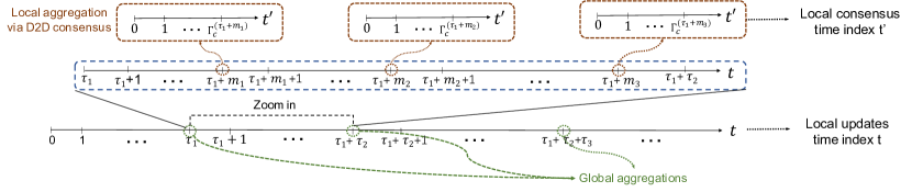
Figure 3: Depiction of two timescales in TT-HF. Time index $t$ captures the local descent iterations and global aggregations. In each local training interval, the nodes will aperiodically engage in consensus procedure. Time index $t^{\prime}$ captures the rounds of these local aggregations.

II-C TT-HF: Two Timescale Hybrid Federated Learning

II-C1 Overview and rationale

TT-HF is comprised of a sequence of local model training intervals in-between aperiodic global aggregations. During each interval, the devices conduct local stochastic gradient descent (SGD) iterations and aperiodically synchronize their model parameters through local consensus procedure within their clusters.

There are three main practical reasons for incorporating the local consensus procedure into the learning paradigm. First, local consensus can help further suppress any bias of device models to their local datasets, which is one of the main challenges faced in federated learning in environments where data may be non-i.i.d. across the network [16]. Second, local D2D communications during the consensus procedure, typically performed over short ranges [51, 52], are expected to incur much lower device power consumption compared with the global aggregations, which require uplink transmissions to potentially far-away aggregation points (e.g., from smartphone to base station). Third, D2D is becoming a prevalent feature of 5G-and-beyond wireless networks [53, 54].

II-C2 TT-HF procedure

We index time as a set of discrete time indices $\mathcal{T}=\{1,2,...\}$. Global aggregation $k$ occurs at time $t_{k}\in\mathcal{T}$ (with $t_{0}=0$), so that $\mathcal{T}_{k}=\{t_{k-1}+1,...,t_{k}\}$ denotes the $k$th local model training interval between aggregations $k-1$ and $k$, of duration $\tau_{k}=t_{k}-t_{k-1}$. Since global aggregations are aperiodic, in general $\tau_{k}\neq\tau_{k^{\prime}}$ for $k\neq k^{\prime}$.

The model computed by the server at the $k$th global aggregation is denoted as $\hat{\mathbf{w}}^{(t_{k})}\in\mathbb{R}^{M}$, which will be defined in (16). The model training procedure starts with the server broadcasting $\hat{\mathbf{w}}^{(0)}$ to initialize the devices’ local models.

Local SGD iterations: Each device $i\in\mathcal{I}$ has its own local model, denoted $\mathbf{w}_{i}^{(t-1)}\in\mathbb{R}^{M}$ at time $t-1$. Device $i$ performs successive local SGD iterations on its model over time. Specifically, at time $t\in\mathcal{T}_{k}$, device $i$ randomly samples a mini-batch $\xi_{i}^{(t-1)}$ of fixed size from its own local dataset $\mathcal{D}_{i}$, and calculates the local gradient estimate

$$\widehat{\mathbf{g}}_{i}^{(t-1)}=\frac{1}{|\xi_{i}^{(t-1)}|}\sum\limits_{(\mathbf{x},y)\in\xi_{i}^{(t-1)}}\nabla\hat{f}(\mathbf{x},y;\mathbf{w}_{i}^{(t-1)}).$$ (9)

It then computes its intermediate updated local model as

$${\widetilde{\mathbf{w}}}_{i}^{(t)}=\mathbf{w}_{i}^{(t-1)}-\eta_{t-1}\widehat{\mathbf{g}}_{i}^{(t-1)},\leavevmode\nobreak\ t\in\mathcal{T}_{k},$$ (10)

where $\eta_{t-1}>0$ denotes the step size. The local model $\mathbf{w}_{i}^{(t)}$ is then updated according to the following consensus-based procedure.

Local model update: At each time $t\in\mathcal{T}_{k}$, each cluster may engage in local consensus procedure for model updating. The decision of whether to engage in this consensus process at time $t$ – and if so, how many iterations of this process to run – will be developed in Sec. IV based on a performance-efficiency trade-off optimization. If the devices do not execute consensus procedure, we have the conventional model update rule ${{\mathbf{w}}}_{i}^{(t)}={\widetilde{\mathbf{w}}}_{i}^{(t)}$ from (10). Otherwise, multiple rounds of D2D communication take place, where in each round parameter transfers occur between neighboring devices. In particular, assuming $\Gamma^{(t)}_{{c}}>0$ rounds for cluster $c$ at time $t$, and letting $t^{\prime}=0,\dots,\Gamma^{(t)}_{{c}}-1$ index the rounds, each node $i\in\mathcal{S}_{c}$ carries out the following for $t^{\prime}=0,\dots,\Gamma^{(t)}_{{c}}-1$:

$$\textbf{z}_{i}^{(t^{\prime}+1)}=v_{i,i}\textbf{z}_{i}^{(t^{\prime})}+\sum_{j\in\mathcal{N}_{i}}v_{i,j}\textbf{z}_{j}^{(t^{\prime})},$$ (11)

where $\textbf{z}_{i}^{(0)}=\widetilde{\mathbf{w}}_{i}^{(t)}$ is the node’s intermediate local model from (10), and $v_{i,j}\geq 0$, $\forall i,j$ is the consensus weight that node $i$ applies to the vector received from $j$. At the end of this process, node $i$ takes $\mathbf{w}_{i}^{(t)}=\textbf{z}_{i}^{(\Gamma^{(t)}_{{c}})}$ as its updated local model.

The index $t^{\prime}$ corresponds to the second timescale in TT-HF, referring to the consensus process, as opposed to the index $t$ which captures the time elapsed by the local gradient iterations. Fig. 3 illustrates these two timescales, where at certain local iterations $t$ the consensus process $t^{\prime}$ is run.

To analyze this update process, we will find it convenient to express the consensus procedure in matrix form. Let $\widetilde{\mathbf{W}}^{(t)}_{{c}}\in\mathbb{R}^{s_{c}\times M}$ denote the matrix of intermediate updated local models of the $s_{c}$ nodes in cluster $\mathcal{S}_{c}$, where the $i$-th row of $\widetilde{\mathbf{W}}^{(t)}_{{c}}$ corresponds to device $i$’s intermediate local model $\widetilde{{\mathbf{w}}}_{i}^{(t)}$. Then, the matrix of updated device parameters after the consensus stage, ${\mathbf{W}}^{(t)}_{{c}}$, can be written as

$$\mathbf{W}^{(t)}_{{c}}=\left(\mathbf{V}_{{c}}\right)^{\Gamma^{(t)}_{{c}}}\widetilde{\mathbf{W}}^{(t)}_{{c}},\leavevmode\nobreak\ t\in\mathcal{T}_{k},$$ (12)

where $\Gamma^{(t)}_{{c}}$ denotes the rounds of D2D consensus in the cluster, and $\mathbf{V}_{{c}}=[v_{i,j}]_{1\leq i,j\leq s_{c}}\in\mathbb{R}^{s_{c}\times s_{c}}$ denotes the consensus matrix, which we characterize further below. The $i$-th row of ${\mathbf{W}}^{(t)}_{{c}}$ corresponds to device $i$’s local update ${{\mathbf{w}}}_{i}^{(t)}$, which is then used in (9) to calculate the gradient estimate for the next local update. For the times $t\in\mathcal{T}_{k}$ where consensus is not used, we set $\Gamma^{(t)}_{{c}}=0$, implying $\mathbf{W}^{(t)}_{{c}}=\widetilde{\mathbf{W}}^{(t)}_{{c}}$ so that devices use their individual gradient updates.

Remark 2.

Note that the graph $G_{c}$ may change over time $t$. In this paper, we only require that the set of devices in each cluster remain fixed during each global aggregation period $k$. We drop the dependency on $t$ for simplicity of presentation, although the analysis implicitly accommodates it. We similarly do so in notations for node and cluster weights $\rho_{i,c}$, $\varrho_{c}$ introduced in Sec. II-B and consensus parameters $v_{i,j}$, $\mathbf{V}_{c}$, $\lambda_{c}$ in Sec. II-C. Assuming a fixed vertex set during each global aggregation period is a practical assumption, especially when the devices move slowly and do not leave the cluster during each local training interval. Moreover, although in the analysis we assume that transmissions are outage- and error-free, in Sec. V we will perform a numerical evaluation to evaluate the impact of fast fading and limited channel state information (CSI), resulting in outages and time-varying link configurations.

Consensus characteristics: The consensus matrix $\mathbf{V}_{{c}}$ can be constructed in several ways based on the cluster topology $G_{c}$. In this paper, we make the following standard assumption [45]:

Assumption 2.

The consensus matrix $\mathbf{V}_{{c}}$ satisfies the following conditions: (i) $\left(\mathbf{V}_{{c}}\right)_{m,n}=0\leavevmode\nobreak\ \leavevmode\nobreak\ \textrm{if}\leavevmode\nobreak\ \leavevmode\nobreak\ \left({m},{n}\right)\notin\mathcal{E}_{{c}}$, i.e., nodes only receive from their neighbors; (ii) $\mathbf{V}_{{c}}\textbf{1}=\textbf{1}$, i.e., row stochasticity; (iii) $\mathbf{V}_{{c}}={\mathbf{V}_{{c}}}^{\top}$, i.e., symmetry; and (iv) $\rho\big{(}\mathbf{V}_{{c}}-\frac{\textbf{1}\textbf{1}^{\top}}{s_{c}}\big{)}<1$, i.e., the largest eigenvalue of $\mathbf{V}_{{c}}-\frac{\textbf{1}\textbf{1}^{\top}}{s_{c}}$ has magnitude $<1$.

For example, from the distributed consensus literature [45], one common choice that satisfies this property is $v_{i,j}=d_{c},\forall j\in\mathcal{N}_{i}$ and $v_{i,i}=1-d_{c}|\mathcal{N}_{i}|$, where $0<d_{{c}}<1/D_{{c}}$ and $D_{{c}}$ denotes the maximum degree among the nodes in $G_{{c}}$.

The consensus procedure process can be viewed as an imperfect aggregation of the models in each cluster. Specifically, we can write the local parameter at device $i\in\mathcal{S}_{c}$ as

$$\mathbf{w}_{i}^{(t)}=\bar{\mathbf{w}}_{c}^{(t)}+\mathbf{e}_{i}^{(t)},$$ (13)

where $\bar{\mathbf{w}}_{c}^{(t)}=\sum_{i\in\mathcal{S}_{c}}\rho_{i,c}\tilde{\mathbf{w}}_{i}^{(t)}$ is the average of the local models in the cluster and $\mathbf{e}_{i}^{(t)}\in\mathbb{R}^{M}$ denotes the consensus error caused by limited D2D rounds (i.e., $\Gamma_{c}^{(t)}<\infty$) among the devices, which can be bounded as in the following lemma.

Input: Length of training $T$, number of global aggregations $K$, D2D rounds $\{\Gamma_{c}^{(t)}\}_{t=1}^{T},\leavevmode\nobreak\ \forall c$, length of local model training intervals $\tau_{k},\leavevmode\nobreak\ k=1,...,K$

Output: Final global model $\hat{\mathbf{w}}^{(T)}$

1 // Initialization by the server

2 Initialize $\hat{\mathbf{w}}^{(0)}$ and broadcast it among the devices along with the indices $n_{c}$ of the sampled devices for the first global aggregation.

3 for $k=1:K$ do

4       for $t=t_{k-1}+1:t_{k}$ do

5             for $c=1:N$ do

6                   // Procedure at the clusters

7                   Each device $i\in\mathcal{S}_{c}$ performs local SGD update based on (9) and (10) using $\mathbf{w}_{i}^{(t-1)}$ to obtain $\widetilde{\mathbf{w}}_{i}^{(t)}$.

8                   Devices inside the cluster conduct $\Gamma^{(t)}_{{c}}$ rounds of consensus procedure based on (11), initializing $\textbf{z}_{i}^{(0)}=\widetilde{\mathbf{w}}_{i}^{(t)}$ and setting $\mathbf{w}_{i}^{(t)}=\textbf{z}_{i}^{(\Gamma^{(t)}_{{c}})}$.

9             end for

10            if $t=t_{k}$ then

11                   // Procedure at the clusters

12                   Each sampled device $n_{c}$ sends $\mathbf{w}_{n_{c}}^{(t_{k})}$ to the server.

13                   // Procedure at the server

14                   Compute $\hat{\mathbf{w}}(t)$ using (16), and broadcast it among the devices along with the indices $n_{c}$ chosen for the next global aggregation.

15             end if

16            

17       end for

18      

19 end for

Algorithm 1 Two timescale hybrid federated learning TT-HF with set control parameters.

Lemma 1.

After performing $\Gamma^{(t)}_{{c}}$ rounds of consensus in cluster $\mathcal{S}_{c}$ with the consensus matrix $\mathbf{V}_{{c}}$, the consensus error $\mathbf{e}_{i}^{(t)}$ satisfies

$$\|\mathbf{e}_{i}^{(t)}\|\leq(\lambda_{{c}})^{\Gamma^{(t)}_{{c}}}\sqrt{s_{c}}\underbrace{\max_{j,j^{\prime}\in\mathcal{S}_{c}}\|\tilde{\mathbf{w}}_{j}^{(t)}-\tilde{\mathbf{w}}_{j^{\prime}}^{(t)}\|}_{\triangleq\Upsilon^{(t)}_{{c}}},\leavevmode\nobreak\ \forall i\in\mathcal{S}_{c}.$$ (14)

where $\lambda_{{c}}=\rho\big{(}\mathbf{V}_{{c}}-\frac{\textbf{1}\textbf{1}^{\top}}{s_{c}}\big{)}$.

Sketch of Proof: Let $\overline{\mathbf{W}}^{(t)}_{{c}}=\frac{1}{s_{c}}\mathbf{1}\mathbf{1}^{\top}\widetilde{\mathbf{W}}^{(t)}_{{c}}$ be the matrix with rows given by the average model parameters across the cluster, and let

$$\mathbf{E}^{(t)}_{{c}}={\mathbf{W}}^{(t)}_{{c}}-\overline{\mathbf{W}}^{(t)}_{{c}}=[\left(\mathbf{V}_{{c}}\right)^{\Gamma^{(t)}_{{c}}}-\mathbf{1}\mathbf{1}^{\top}/s_{c}][\widetilde{\mathbf{W}}^{(t)}_{{c}}-\overline{\mathbf{W}}^{(t)}_{{c}}],$$

so that $[\mathbf{E}^{(t)}_{{c}}]_{i,:}$ ($i$th row of $\mathbf{E}^{(t)}_{{c}}$) $=\mathbf{e}_{i}^{(t)}$, where in the second step we used (12) and the fact that $\mathbf{1}^{\top}\mathbf{E}^{(t)}_{{c}}=\mathbf{0}$ (hence $\mathbf{E}^{(t)}_{{c}}=[\mathbf{I}-\mathbf{1}\mathbf{1}^{\top}/s_{c}]\mathbf{E}^{(t)}_{{c}}$). Therefore, using Assumption 2, we can bound the consensus error as

$$\|\mathbf{e}_{i}^{(t)}\|^{2}\leq\mathrm{trace}((\mathbf{E}^{(t)}_{{c}})^{\top}\mathbf{E}^{(t)}_{{c}})$$ (15)

$$=\mathrm{trace}\Big{(}[\widetilde{\mathbf{W}}^{(t)}_{{c}}{-}\overline{\mathbf{W}}^{(t)}_{{c}}]^{\top}[\left(\mathbf{V}_{{c}}\right)^{\Gamma^{(t)}_{{c}}}{-}\mathbf{1}\mathbf{1}^{\top}/s_{c}]^{2}[\widetilde{\mathbf{W}}^{(t)}_{{c}}{-}\overline{\mathbf{W}}^{(t)}_{{c}}]\Big{)}$$

$$\leq(\lambda_{{c}})^{2\Gamma^{(t)}_{{c}}}\sum_{j=1}^{s_{c}}\|\tilde{\mathbf{w}}_{j}^{(t)}-\bar{\mathbf{w}}_{c}^{(t)}\|^{2}$$

$$\leq(\lambda_{{c}})^{2\Gamma^{(t)}_{{c}}}\frac{1}{s_{c}}\sum_{j,j^{\prime}=1}^{s_{c}}\|\tilde{\mathbf{w}}_{j}^{(t)}-\tilde{\mathbf{w}}_{j^{\prime}}^{(t)}\|^{2}$$

$$\leq(\lambda_{{c}})^{2\Gamma^{(t)}_{{c}}}s_{c}\max_{j,j^{\prime}\in\mathcal{S}_{c}}\|\tilde{\mathbf{w}}_{j}^{(t)}-\tilde{\mathbf{w}}_{j^{\prime}}^{(t)}\|^{2},$$

so that the result directly follows. For the complete proof, refer to Appendix D. $\blacksquare$

Note that $\Upsilon^{(t)}_{{c}}$ defined in (14) captures the divergence of intermediate updated local model parameters in cluster $\mathcal{S}_{c}$ at time $t\in\mathcal{T}_{k}$ (before consensus is performed). Intuitively, according to (14), to make the consensus error smaller, more rounds of consensus need to be performed. However, this may be impractical due to energy and delay considerations, hence a trade-off arises between the consensus error and the energy/delay cost. This trade-off will be optimized by tuning $\Gamma_{c}^{(t)}$, via our adaptive control algorithm developed in Sec. IV.

Global aggregation: At the end of each local model training interval $\mathcal{T}_{k}$, the global model $\mathbf{w}$ will be updated based on the trained local model updates. Referring to Fig. 2, the main server will sample one device from each cluster $c$ uniformly at random, and request these devices to upload their local models, so that the new global model is updated as

$$\hat{\mathbf{w}}^{(t)} =\sum\limits_{c=1}^{N}\varrho_{c}\mathbf{w}_{n_{c}}^{(t)},\;\;t=t_{k},k=1,2,...$$ (16)

where $n_{c}$ is the node sampled from cluster $c$ at time $t$. This sampling technique is introduced to reduce the uplink communication cost by a factor of the cluster sizes, and is enabled by the consensus procedure, which mimics a local aggregation procedure within a cluster (albeit imperfectly due to consensus errors, see (13)) [18]. The global model is then broadcast by the main server to all of the edge devices, which override their local models at time $t_{k}$: $\mathbf{w}_{i}^{(t_{k})}=\hat{\mathbf{w}}^{(t_{k})}$, $\forall i$. The process then repeats for $\mathcal{T}_{k+1}$.

A summary of the TT-HF algorithm developed in this section (for set control parameters) is given in Algorithm 1.

Remark 3.

Note that we consider digital transmission (in both D2D and uplink/downlink communications) where using state-of-the-art techniques in encoding/decoding, e.g., low density parity check (LDPC) codes, the bit error rate (BER) is reasonably small and negligible [55]. Moreover, the effect of quantized model transmissions can be readily incorporated using techniques developed in [44], and precoding techniques may be used to mitigate the effect of signal outage due to fading [56]. Therefore, in this analysis, we assume that the model parameters transmitted by the devices to their neighbors (during consensus) and then to the server (during global aggregation) are received with no errors at the respective receivers. The impact of outages due to fast fading and lack of CSI will be studied numerically in Sec. V.

III Convergence Analysis of TT-HF

In this section, we theoretically analyze the convergence behavior of TT-HF. Our main results are presented in Sec. III-B and Sec. III-C. Before then, in Sec. III-A, we introduce some additional definitions and a key proposition for the analysis.

III-A Definitions and Bounding Model Dispersion

We first introduce a standard assumption on the noise of gradient estimation, and then define an upper bound on the average of consensus error for the clusters:

Assumption 3.

Let ${\mathbf{n}}_{i}^{(t)}{=}\widehat{\mathbf{g}}_{i}^{(t)}{-}\nabla F_{i}(\mathbf{w}_{i}^{(t)})$ $\forall i,t$ denote the noise of the estimated gradient through the SGD process for device $i$. We assume that it is unbiased with bounded variance, i.e. $\mathbb{E}[{\mathbf{n}}_{i}^{(t)}|\mathbf{w}_{i}^{(t)}]{=}0$ and $\exists\sigma{>}0{:}\leavevmode\nobreak\ \mathbb{E}[\|{\mathbf{n}}_{i}^{(t)}\|^{2}|\mathbf{w}_{i}^{(t)}]{\leq}\sigma^{2}$, $\forall i,t$.

Moreover, the following condition bounds the consensus error within each cluster.

Condition 1.

Let $\epsilon_{c}^{(t)}$ be an upper bound on the average of the consensus error inside cluster $c$ at time $t$, i.e.,

$$\frac{1}{s_{c}}\sum\limits_{i\in\mathcal{S}_{c}}\|\mathbf{e}_{i}^{(t)}\|^{2}\leq(\epsilon_{c}^{(t)})^{2}.$$ (17)

We further define $(\epsilon^{(t)})^{2}=\sum\limits_{c=1}^{N}\rho_{c}(\epsilon_{c}^{(t)})^{2}$ as the average of these upper bounds over the network at time $t$.

In fact, using Lemma 1, this condition can be satisfied by tuning the number of consensus steps. In our analysis, we will derive conditions on $\epsilon_{c}^{(t)}$ that are sufficient to guarantee convergence of TT-HF (see Proposition 1).

We next define the expected variance in models across clusters at a given time, which we refer to as model dispersion:

Definition 2.

We define the expected model dispersion across the clusters at time $t$ as

$$A^{(t)}=\mathbb{E}\left[\sum\limits_{c=1}^{N}\varrho_{c}\big{\|}\bar{\mathbf{w}}_{c}^{(t)}-\bar{\mathbf{w}}^{(t)}\big{\|}^{2}\right],$$ (18)

where $\bar{\mathbf{w}}_{c}^{(t)}$ is defined in (13) and $\bar{\mathbf{w}}^{(t)}=\sum\limits_{c=1}^{N}\varrho_{c}\bar{\mathbf{w}}_{c}^{(t)}$ is the global average of the local models at time $t$.

$A^{(t)}$ measures the degree to which the cluster models deviate from their average throughout the training process. Obtaining an upper bound on this quantity is non-trivial due to the coupling between the gradient diversity and the model parameters imposed by (7). For an appropriate choice of step size in (10), we upper bound this quantity at time $t$ through a set of new techniques that include the mathematics of coupled dynamic systems. Specifically, we have the following result:

Proposition 1.

If $\eta_{t}=\frac{\gamma}{t+\alpha}$ for some $\gamma>0$, $\epsilon^{(t)}$ is non-increasing for $t\in\mathcal{T}_{k}$, i.e., $\epsilon^{(t+1)}\leq\epsilon^{(t)}$, and $\alpha\geq\gamma\beta\max\{\lambda_{+}-2+\frac{\mu}{2\beta},\frac{\beta}{\mu}\}$, then

$$A^{(t)}\leq \frac{16\omega^{2}}{\mu}(\Sigma_{+,t})^{2}[F(\bar{\mathbf{w}}(t_{k-1}))-F(\mathbf{w}^{*})]$$

$$+25(\Sigma_{+,t})^{2}\left(\frac{\sigma^{2}+\delta^{2}}{\beta^{2}}+(\epsilon^{(0)})^{2}\right),\leavevmode\nobreak\ \leavevmode\nobreak\ t\in\mathcal{T}_{k},$$ (19)

where

and $\lambda_{+}=1-\frac{\mu}{4\beta}+\sqrt{(1+\frac{\mu}{4\beta})^{2}+2\omega}.$

Proof.

See Appendix A. ∎

The bound in (1) demonstrates how the expected model dispersion across the clusters increases with respect to the consensus error ($\epsilon^{(0)}$), the noise in the gradient estimation ($\sigma^{2}$), and the heterogeneity of local datasets ($\delta,\omega$). Intuitively, the upper bound in (1) dictates that, the larger $\epsilon^{(0)}$, $\sigma^{2}$, $\delta$ or $\omega$, the larger the dispersion, due to error propagation in the network. Proposition 1 will be an instrumental result in the convergence proof developed in the next section.

III-B General Convergence Behavior of $\hat{\mathbf{w}}^{(t)}$

Next, we focus on the convergence of the global loss. In the following theorem, we bound the expected distance that the global loss is from the optimal over time, as a function of the model dispersion.

Theorem 1.

When using TT-HF for ML model training with $\eta_{t}\leq 1/\beta$ $\forall t$, the one-step behavior of the global model $\hat{\mathbf{w}}^{(t)}$ (see (16)) satisfies, for $t\in\mathcal{T}_{k}$,

$$\mathbb{E}\left[F(\hat{\mathbf{w}}^{(t+1)})-F(\mathbf{w}^{*})\right]\leq\underbrace{(1-\mu\eta_{t})\mathbb{E}[F(\hat{\mathbf{w}}^{(t)})-F(\mathbf{w}^{*})]}_{{(a)}}$$

$$+\underbrace{\frac{\eta_{t}\beta^{2}}{2}A^{(t)}+\frac{1}{2}[\eta_{t}\beta^{2}(\epsilon^{(t)})^{2}+\eta_{t}^{2}\beta\sigma^{2}+\beta(\epsilon^{(t+1)})^{2}]}_{(b)},$$ (20)

where $A^{(t)}$ is the model dispersion from Definition 2.

Proof.

See Appendix B. ∎

Theorem 1 quantifies the dynamics of the global model relative to the optimal model during a given update period $\mathcal{T}_{k}$ of TT-HF. Since the theorem holds for all $t\in\mathcal{T}_{k}$, it also quantifies the suboptimality gap when global aggregation is performed at time $t+1=t_{k}$. Note that the term (a) corresponds to the one-step progress of a centralized gradient descent under strongly-convex global loss (Assumption 1), so that the term (b) quantifies the additional loss incurred as a result of the model dispersion across the clusters ($A^{(t)}$, which in turn is bounded by Proposition 1), consensus errors ($\epsilon^{(t)}$), and SGD noise ($\sigma^{2}$). In fact, without careful choice of our control parameters, the sequence $\mathbb{E}[F(\hat{\mathbf{w}}^{(t)})-F(\mathbf{w}^{*})]$ may diverge. Thus, we are motivated to find conditions under which convergence is guaranteed, and furthermore, under which the upper bound in (1) will approach zero.

Specifically, we aim for TT-HF to match the asymptotic convergence behavior of centralized stochastic gradient descent (SGD) under a diminishing step size, which is $\mathcal{O}(1/t)$ [57]. From (1), we see that to match SGD, the terms in $(b)$ should be of order $\mathcal{O}(\eta_{t}^{2})$, i.e., the same as the degradation due to the SGD noise, $\eta_{t}^{2}\beta\sigma^{2}/2$. This implies that control parameters need to be tuned in such a way that $A^{(t)}{=}\mathcal{O}(\eta_{t})$ and $\epsilon^{(t)}{=}\mathcal{O}(\eta_{t})$. Proving that these conditions hold under proper choice of parameters will be part of Theorem 2.

III-C Sublinear Convergence Rate of $\hat{\mathbf{w}}^{(t)}$

Among the quantities involved in Theorem 1, $\eta_{t},\tau_{k}$ and $\epsilon^{(t)}$ are the three tunable parameters that directly impact the learning performance of TT-HF. We now prove that with proper choice of these parameters, TT-HF enjoys sub-linear convergence with rate of $\mathcal{O}(1/t)$.

Theorem 2.

Under Assumptions 1, 2, and 3, suppose $\eta_{t}=\frac{\gamma}{t+\alpha}$ and $\epsilon^{(t)}=\eta_{t}\phi$, where $\gamma>1/\mu$, $\phi>0$, $\alpha\geq\alpha_{\min}$ and $\omega<\omega_{\max}(\alpha)$. Then, by using TT-HF for ML model training,

$$\mathbb{E}\left[F(\hat{\mathbf{w}}^{(t)})-F(\mathbf{w}^{*})\right]\leq\frac{\nu}{t+\alpha},\leavevmode\nobreak\ \leavevmode\nobreak\ \forall t,$$ (21)

where $\tau=\max_{1\leq\ell\leq k}\{\tau_{\ell}\}$,

$$\alpha_{\min}\triangleq\gamma\beta\max\Big{\{}\frac{\mu}{4\beta}-1+\sqrt{(1+\frac{\mu}{4\beta})^{2}+2\omega},\frac{\beta}{\mu}\Big{\}},$$ (22)

$$\omega_{\max}(\alpha)\triangleq\frac{1}{\beta\gamma}\sqrt{\frac{\alpha}{Z_{1}}}\sqrt{\mu\gamma-1+\frac{1}{1+\alpha}},$$ (23)

$$\nu{\triangleq}\max\left\{\frac{\beta^{2}\gamma^{2}Z_{2}}{\mu\gamma-1},\frac{\alpha Z_{2}/Z_{1}}{\omega_{\max}^{2}{-}\omega^{2}},\alpha\left[F(\hat{\mathbf{w}}^{(0)}){-}F(\mathbf{w}^{*})\right]\right\},\!\!\!$$ (24)

$$Z_{1} =\frac{32\beta^{2}\gamma}{\mu}(\tau-1)\left(1+\frac{\tau}{\alpha-1}\right)^{2}\left(1+\frac{\tau-1}{\alpha-1}\right)^{6\beta\gamma}$$ (25)

$$Z_{2}=\frac{\sigma^{2}+2\phi^{2}}{2\beta}+50\gamma(\tau-1)\left(1+\frac{\tau-2}{\alpha+1}\right)$$

$$\qquad\times\left(1+\frac{\tau-1}{\alpha-1}\right)^{6\beta\gamma}\left(\sigma^{2}+\phi^{2}+\delta^{2}\right).$$ (26)

Proof.

See Appendix C. ∎

Theorem 2 is one of the central contributions of this paper, revealing how several parameters (some controllable and others characteristic of the environment) affect the convergence of TT-HF, and conditions under which $\mathcal{O}(1/t)$ convergence can be achieved. We make several key observations. First, to achieve $\mathcal{O}(1/t)$ convergence, the gradient diversity parameter $\omega=\frac{\zeta}{2\beta}$ should not be too large ($\omega<\omega_{\max}(\alpha)$); in fact, $\omega$ induces error propagation of order $\sim\|\mathbf{w}_{c}-\mathbf{w}^{*}\|$, so that too large values of $\omega$ may cause the error to diverge. Since $\omega_{\max}(\alpha)$ is an increasing function of $\alpha$ (see (23)), larger values of $\omega$ may be tolerated by increasing $\alpha$, i.e., by using a smaller step-size $\eta_{t}$, confirming the intuition that larger gradient diversity requires a smaller step-size for convergence. However, the penalty incurred may be slower convergence of the suboptimality gap (since $\nu$ increases with $\alpha$, see (24)).

We now discuss the choice of the consensus error $\epsilon^{(t)}$. To guarantee $\mathcal{O}(1/t)$ convergence, Theorem 2 dictates that it should be chosen as $\epsilon^{(t)}=\eta_{t}\phi$ for a constant $\phi>0$, i.e. it should decrease over time according to the step-size. To see that this is a feasible and practical condition, note from Lemma 1 that the upper bound of $\|\mathbf{e}_{i}^{(t)}\|$ increases proportionally to the divergence $\Upsilon^{(t)}_{c}$ (see (14)), and decreases at geometric rate with the number of consensus steps. In turn, $\Upsilon^{(t)}_{c}$ can be shown to be of the order of the step-size $\eta_{t}$ (assuming $\eta_{t}\approx\eta_{t-1}$):

$$\Upsilon^{(t)}_{{c}}=\max_{j,j^{\prime}\in\mathcal{S}_{c}}\|\widetilde{\mathbf{w}}^{(t)}_{{j}}-\widetilde{\mathbf{w}}^{(t)}_{{j^{\prime}}}\|\approx\eta_{t}\max_{j,j^{\prime}\in\mathcal{S}_{c}}\big{\|}\widehat{\mathbf{g}}_{j}^{(t-1)}-\widehat{\mathbf{g}}_{j^{\prime}}^{(t-1)}\big{\|},$$

where we used (10), and the approximation holds if we assume the difference ${\mathbf{w}}^{(t-1)}_{{j}}-{\mathbf{w}}^{(t-1)}_{{j^{\prime}}}$ in initial model parameters at $t-1$ is negligible compared to the gradients. This is a legit assumption, since ${\mathbf{w}}^{(t-1)}_{{j}}$ is the model parameter at node $j$, after the consensus rounds at time $t-1$. Using Lemma 1, it then follows that, to make $\epsilon^{(t)}=\eta_{t}\phi$, the number of consensus rounds should be chosen such that $(\lambda_{{c}})^{\Gamma^{(t)}_{{c}}}\approx\frac{1}{\sqrt{s_{c}}}\phi/\max_{j,j^{\prime}\in\mathcal{S}_{c}}\big{\|}\widehat{\mathbf{g}}_{j}^{(t-1)}-\widehat{\mathbf{g}}_{j^{\prime}}^{(t-1)}\big{\|}$, and are thus dominated by the divergence of local gradients within the cluster and SGD noise, irrespective of the step-size. We will use this property in the development of our control algorithm for $\Gamma^{(t)}_{c}$ in Sec. IV.

The bound also shows the impact of the duration of local model training intervals $\tau$ on the convergence, through the term $\nu$ in (21). In particular, from (24), it can be seen that increasing $\tau$ results in a sharp increase of $\nu$ (through the factors $Z_{1}$ and $Z_{2}$ defined in (25) and (26)). Moreover, we also observe a quadratic impact on $\nu$ with respect to the consensus error $\epsilon^{(t)}$ (through $\phi$). It then follows that, all else constant, increasing the value of $\tau$ requires a smaller value of $\phi$ (i.e., more accurate consensus) to achieve a desired value of $\nu$ in (24). This is consistent with how TT-HF is designed, since the motivation for including consensus rounds (to decrease $\epsilon^{(t)}$) is to reduce the global aggregation frequency, which results in uplink bandwidth utilization and power consumption savings.

These observations reveal a trade-off between accuracy, delay, and energy consumption. In the next section, we leverage these relationships in developing an adaptive algorithm for TT-HF that tunes the control parameters to achieve the convergence bound in Theorem 2 while minimizing network costs.

IV Adaptive Control Algorithm for TT-HF

There are three parameters in TT-HF that can be tuned over time: (i) local model training intervals $\tau_{k}$, (ii) gradient descent step size $\eta_{t}$, and (iii) rounds of D2D communications $\Gamma_{c}^{(t)}$. In this section, we develop a control algorithm (Sec. IV-D) based on Theorem 2 for tuning (i), (ii) at the main server at the beginning of each global aggregation, and (iii) at each device cluster in a decentralized manner. To do so, we propose an approach for determining the learning-related parameters (Sec. IV-A), a resource-performance tradeoff optimization for $\tau_{k}$ and $\Gamma_{c}^{(t)}$ (Sec. IV-B), and estimation procedures for dataset-related parameters (Sec. IV-C).

IV-A Learning-Related Parameters ($\alpha,\gamma,\phi$, $\eta_{t}$)

We aim to tune the step size-related parameters ($\alpha,\gamma$) and the consensus error coefficient ($\phi$) to satisfy the conditions in Theorem 2. In this section, we present a method for doing so given properties of the ML model, local datasets, and SGD noise ($\beta,\mu,\zeta,\delta,\sigma$, and thus $\omega=\zeta/(2\beta)$). Later in Sec. IV-C, we will develop methods for estimating $\zeta,\delta,\sigma$ at the server. We assume that the latency-sensitivity of the learning application specifies a tolerable amount of time that TT-HF can wait between consecutive global aggregations, i.e., the value of $\tau$.

To tune the step size parameters, first, a value of $\gamma$ is determined such that $\gamma>1/\mu$. Then, since smaller values of $\alpha$ are associated with faster convergence, the minimum value of $\alpha$ that simultaneously satisfies the conditions in the statement of Theorem 2 is chosen, i.e., $\alpha\geq\alpha_{\min}$ and $\omega_{\max}>\omega$ (note that $\omega_{\max}$ is a function of $\alpha$, see (23).

Let $T$ be a (maximum) desirable duration of the entire TT-HF algorithm, and $\xi$ be a (maximum) desirable loss at the end of the model training, which may be chosen based on the learning application. To satisfy the loss requirement, from Theorem 2 the following condition needs to be satisfied,

$$\frac{\nu}{T+\alpha}\leq\xi,$$ (27)

yielding a maximum value tolerated for $\nu$, i.e., $\nu^{\mathsf{max}}=\xi(T+\alpha)$. Since $\nu$ is a function of the local model training period $\tau$ and consensus coefficient $\phi$ (see (24)), this bound places a condition on the parameters $\tau$ and $\phi$. Furthermore, with the values of $\alpha$ and $\gamma$ chosen above, along with the value of $\tau$, the algorithm may not always be able to provide any arbitrary desired loss $\xi$ at time $T$. Therefore, considering the expression for $\nu$ from Theorem 2, the following feasibility check is conducted:

where

$$Z^{\mathsf{min}}_{2}=\frac{\sigma^{2}}{2\beta}+50\gamma(\tau-1)\Big{(}1+\frac{\tau-2}{\alpha+1}\Big{)}\Big{(}1+\frac{\tau-1}{\alpha-1}\Big{)}^{6\beta\gamma}\big{(}\sigma^{2}+\delta^{2}\big{)}$$

is the value of $Z_{2}$ obtained by setting the consensus coefficient $\phi=0$ in (26). The third term inside the $\max$ of (28) is obtained via the Polyak-Lojasiewicz inequality $\left\|\nabla F(\hat{\mathbf{w}}^{(t)})\right\|^{2}\geq 2\mu[F(\hat{\mathbf{w}}^{(t)})-F(\mathbf{w}^{*})]$, since the value of $F(\mathbf{w}^{*})$ is not known, whereas $\nabla F(\hat{\mathbf{w}}^{(t)})$ can be estimated using the local gradient of the sampled devices at the server. If (28) is not satisfied, the chosen values of $\tau$, $\xi$ and/or $T$ must be loosened, and this procedure must be repeated until (28) becomes feasible.

Once $\alpha,\gamma$ and $\tau$ are chosen, we move to selecting $\phi$. All else constant, larger consensus errors would be more favorable in TT-HF due to requiring less rounds of D2D communications (Lemma 1). The largest possible value of $\phi$, denoted $\phi^{\mathsf{max}}$, can be obtained directly from (28) via replacing $Z_{2}^{\mathsf{min}}$ with $Z_{2}$ and considering the definition of $Z_{2}$ in (26):

$$\phi^{\mathsf{max}}=\sqrt{\beta}\sqrt{\frac{\nu^{\mathsf{max}}\min\left\{\frac{\mu\gamma-1}{\beta^{2}\gamma^{2}},\frac{Z_{1}\left(\omega_{\max}^{2}-\omega^{2}\right)}{\alpha}\right\}-Z_{2}^{\mathsf{min}}}{1+50\beta\gamma(\tau-1)\left(1+\frac{\tau-2}{\alpha+1}\right)\left(1+\frac{\tau-1}{\alpha-1}\right)^{6\beta\gamma}}}.$$ (29)

Note that (29) exists if the feasibility check in (28) is satisfied.

The values of $\nu^{\mathsf{max}}$ and $\alpha$ are re-computed at the server at each global aggregation. The devices use this to set their step sizes $\eta_{t}$ during the next local update period accordingly.

IV-B Local Training Periods ($\tau_{k}$) and Consensus Rounds ($\Gamma^{(t)}_{c}$)

One of the main motivations behind TT-HF is minimizing the resource consumption among edge devices during model training. We thus propose tuning the $\tau_{k}$ and $\Gamma^{(t)}_{c}$ parameters according to the joint impact of three metrics: energy consumption, training delay imposed by consensus, and trained model performance. To capture this trade-off, we formulate an optimization problem $(\bm{\mathcal{P}})$ solved by the main server at the beginning of each global aggregation period $\mathcal{T}_{k}$, i.e., when $t=t_{k-1}$:

$$(\bm{\mathcal{P}}):\leavevmode\nobreak\ \leavevmode\nobreak\ \min_{\tau_{k}}\underbrace{\frac{c_{1}\Big{(}E_{\textrm{Glob}}+\sum\limits_{t=t_{k-1}}^{t_{k-1}+\tau_{k}}\sum\limits_{c=1}^{N}\Gamma_{c}^{(t)}s_{c}E_{\textrm{D2D}}\Big{)}}{\tau_{k}}}_{(a)}+$$

$$\!\!\!\!\underbrace{\frac{c_{2}\Big{(}\Delta_{\textrm{Glob}}+\sum\limits_{t=t_{k-1}}^{t_{k-1}+\tau_{k}}\sum\limits_{c=1}^{N}\Gamma_{c}^{(t)}\Delta_{\textrm{D2D}}\Big{)}}{{\tau_{k}}}}_{(b)}+c_{3}\Big{(}\underbrace{1-\frac{t_{k-1}+\alpha}{t_{k-1}+\tau_{k}+\alpha}}_{(c)}\Big{)}$$

s.t.

$$\;\;\;\Gamma_{c}^{(t)}=\max\Big{\{}\Big{\lceil}\log\Big{(}\frac{\eta_{t}\phi}{\sqrt{s_{c}}\Upsilon_{c}^{(t)}}\Big{)}/\log\Big{(}\lambda_{c}\Big{)}\Big{\rceil},0\Big{\}},\forall c,$$ (30)

$$\;\;\;1\leq\tau_{k}\leq\min{\{\tau,T-t_{k-1}\}},\tau_{k}\in\mathbb{Z}^{+},$$ (31)

$$\;\;\;\Upsilon_{c}^{(t_{k-1})}=0,\leavevmode\nobreak\ \forall c,$$ (32)

$$\;\;\;\Upsilon_{c}^{(t)}=\mathbbm{1}_{\{\Gamma^{(t-1)}_{c}=0\}}(\underbrace{A_{c}^{(k)}\Upsilon_{c}^{(t-1)}+B_{c}^{(k)}}_{(d)})\;+$$

$$\leavevmode\nobreak\ \leavevmode\nobreak\ \leavevmode\nobreak\ \leavevmode\nobreak\ \leavevmode\nobreak\ \leavevmode\nobreak\ \leavevmode\nobreak\ \leavevmode\nobreak\ \leavevmode\nobreak\ \leavevmode\nobreak\ \leavevmode\nobreak\ \left(1-\mathbbm{1}_{\{\Gamma^{(t-1)}_{c}=0\}}\right)(\underbrace{a_{c}^{(k)}\Upsilon_{c}^{(t-1)}+b_{c}^{(k)}}_{(e)}),\leavevmode\nobreak\ \forall c,$$ (33)

where $E_{\textrm{D2D}}$ is the energy consumption of each D2D communication round for each device, $E_{\textrm{Glob}}$ is the energy consumption for device-to-server communications, $\Delta_{\textrm{D2D}}$ is the communication delay per D2D round conducted in parallel among the devices, and $\Delta_{\textrm{Glob}}$ is the device-to-server communication delay. The objective function captures the trade-off between average energy consumption (term $(a)$), average D2D delay (term $(b)$), and expected ML model performance (term $(c)$). In particular, term $(c)$ is a penalty on the ratio of the upper bound given in (21) between the updated model and the previous model at the main server. A larger ratio implies the difference in performance between the aggregations is smaller, and thus that synchronization is occurring frequently, consistent with $\tau_{k}$ appearing in the denominator. This term also contains a diminishing marginal return from global aggregations as the learning proceeds: smaller values of $\tau_{k}$ are more favorable in the initial stages of ML model training, i.e., for smaller $t_{k-1}$. This matches well with the intuition that ML model performance has a sharper increase at the beginning of model training, so frequent aggregations at smaller $t_{k-1}$ will have larger benefit to the model performance stored at the main server. The coefficients $c_{1},c_{2},c_{3}\geq 0$ are introduced to weigh each of the design considerations.

The equality constraint on $\Gamma^{(t)}_{c}$ in (30) forces the condition $\epsilon^{(t)}=\eta_{t}\phi$ imposed by Theorem 2, obtained using the result in Lemma 1. This equality reveals the condition under which the local aggregations, i.e., D2D communication, are triggered. Note that since the spectral radius is less than one, we have $\log(\lambda_{c})<0$, thus the requirement to conduct D2D communications, i.e., triggering in cluster model synchronization, is $\sqrt{s_{c}}\Upsilon_{c}^{(t)}>\eta\phi$. In other words, when the divergence of local models exceeds a predefined threshold $\Upsilon_{c}^{(t)}>\frac{\eta\phi}{\sqrt{s_{c}}}$, local synchronization is triggered via D2D communication, and the number of D2D rounds is given by $\Gamma_{c}^{(t)}$. Also,  (31) ensures the feasible ranges for $\tau_{k}$.

As can be seen from (30), to obtain the desired consensus rounds for future times $t\in\mathcal{T}_{k}$, the values of $\Upsilon_{c}^{(t)}$ – the divergence of model parameters in each cluster – are needed. Obtaining these exact values at $t=t_{k-1}$ is not possible since it requires the knowledge of the model parameters $\widetilde{\mathbf{w}}_{i}^{(t)}$ of the devices for the future timesteps, which is non-causal. To address this challenge, problem $(\bm{\mathcal{P}})$ incorporates the additional constraints (32) and (33), which aim to estimate the future values of $\Upsilon^{(t)}_{c}$, $\forall c$ through a time-series predictor, initialized as $\Upsilon_{c}^{(t_{k-1})}=0$ in (32) (since, at the beginning of the period, the nodes start with the same model provided by the server). In the expression (33), $\mathbbm{1}_{\{\Gamma^{(t-1)}_{c}=0\}}$ takes the value of $1$ when no D2D communication rounds are performed at $t-1$, and $0$ otherwise. Two linear terms ($(d)$ and $(e)$) are included, one for each of these cases, characterized by coefficients $A_{c}^{(k)},B_{c}^{(k)},a_{c}^{(k)},b_{c}^{(k)}\in\mathbb{R}$ which vary across clusters and global aggregations. These coefficients are estimated through fitting the linear functions to the values of $\Upsilon_{c}^{(t)}$ obtained from the previous global aggregation $\mathcal{T}_{k-1}$. These values of $\Upsilon_{c}^{(t)}$ from $\mathcal{T}_{k-1}$ are in turn estimated in a distributed manner through a method presented in Sec. IV-C.

Note that $(\bm{\mathcal{P}})$ is a non-convex and integer optimization problem. Given the parameters in Sec. IV-A, the solution for $\tau_{k}$ can be obtained via a line search over the integer values in the range of $\tau_{k}$ given in (31). Solving our optimization problem involves two steps: (i) linear regression of the constants used in (53), i.e., $A_{c}^{(k)},B_{c}^{(k)},a_{c}^{(k)},b_{c}^{(k)}$ using the history of observations, and (ii) line search over the feasible integer values for $\tau_{k}$. The complexity of part (i) is $\mathcal{O}(\tau_{k-1})$, since the dimension of each observant, i.e., $\Upsilon_{c}^{(t)}$, is one and the observations are obtained via looking back into the previous global aggregation interval. Also, the complexity of (ii) is $\mathcal{O}(\tau_{\max})$ since it is just an exhaustive search over the range of $\tau\leq\tau_{\max}$, where $\tau_{\max}$ is the maximum tolerable interval that satisfies the feasibility conditions in Sec. IV-A. While the optimization produces predictions of $\Gamma^{(t)}_{c}$ for $t\in\mathcal{T}_{k}$ through (30), the devices will later compute (30) at time $t$ when the real-time estimates of $\Upsilon^{(t)}_{c}$ can be made through (IV-C2), as will be discussed next.

IV-C Data and Model-Related Parameters ($\delta,\zeta,\sigma^{2},\Upsilon^{(t)}_{c}$)

We also need techniques for estimating the gradient diversity ($\delta$, $\zeta$), SGD noise ($\sigma^{2}$), and cluster parameter divergence ($\Upsilon^{(t)}_{c}$).

IV-C1 Estimation of $\delta,\zeta,\sigma^{2}$

These parameters can be estimated by the main server during model training. The server can estimate $\delta$ and $\zeta$ at each global aggregation by receiving the latest gradients from SGD at the sampled devices. $\sigma^{2}$ can first be estimated locally at the sampled devices, and then decided at the main server.

Specifically, to estimate $\delta,\zeta$, since the value of $\mathbf{w}^{*}$ is not known, we upper bound the gradient diversity in Definition 1 by introducing a new parameter $\delta^{\prime}$:

$$\|\nabla\hat{F}_{c}(\mathbf{w})-\nabla F(\mathbf{w})\|\leq\delta+\zeta\|\mathbf{w}-\mathbf{w}^{*}\|\leq\delta^{\prime}+\zeta\|\mathbf{w}\|,$$ (34)

which satisfies $\delta^{\prime}\geq\delta+\zeta\|\mathbf{w}^{*}\|$. Thus, a value of $\zeta<2\beta$ is set, and then the value of $\delta^{\prime}$ is estimated using (34), where the server uses the SGD gradients $\widehat{\mathbf{g}}_{n_{c}}^{(t_{k})}$ from the sampled devices $n_{c}$ at the instance of each global aggregation $k$, and chooses the smallest $\delta^{\prime}$ such that $\|\nabla\hat{F}_{c}(\hat{\mathbf{w}}^{(t_{k})})-\nabla F(\hat{\mathbf{w}}^{(t_{k})})\|\approx\|\widehat{\mathbf{g}}_{n_{c}}^{(t_{k})}-\sum_{c^{\prime}=1}^{N}\varrho_{c^{\prime}}\widehat{\mathbf{g}}_{n_{c^{\prime}}}^{(t_{k})}\|\leq\delta^{\prime}+\zeta\|\hat{\mathbf{w}}^{(t_{k})}\|$ $\forall c$.

From Assumption 3, a simple way of obtaining the value of $\sigma^{2}$ would be comparing the gradients from sampled devices with their full-batch counterparts. But this might be impractical if the local datasets $\mathcal{D}_{i}$ are large. Thus, we propose an approach where $\sigma^{2}$ is computed at each device through two independent mini-batches of data. Recall $|\xi_{i}|$ denotes the mini-batch size used at node $i$ during the model training. At each instance of global aggregation, the sampled devices each select two mini-batches of size $|\xi_{i}|$ and compute two SGD realizations $\mathbf{g}_{1}$, $\mathbf{g}_{2}$ from which $\widehat{\mathbf{g}}_{i}^{(t_{k})}=(\mathbf{g}_{1}+\mathbf{g}_{2})/2$. Since $\mathbf{g}_{1}=\nabla F_{i}(\mathbf{w}^{(t_{k})})+\mathbf{n}_{1}$, $\mathbf{g}_{2}=\nabla F_{i}(\mathbf{w}^{(t_{k})})+\mathbf{n}_{2}$, we use the fact that $\mathbf{n}_{1}$ and $\mathbf{n}_{2}$ are independent random variables with the same upper bound on variance $\sigma^{2}$, and thus $\|\mathbf{g}_{1}-\mathbf{g}_{2}\|^{2}=\|\mathbf{n}_{1}-\mathbf{n}_{2}\|^{2}\leq 2\sigma^{2}$, from which $\sigma^{2}$ can be approximated locally. These scalars are then transferred to the main server, which in turn chooses the maximum reported $\sigma^{2}$ from the sampled devices.

IV-C2 Estimation of $\Upsilon^{(t)}_{c}$

Based on (14), we propose the following approximation to estimate the value of $\Upsilon^{(t)}_{c}$:

$$\Upsilon^{(t)}_{c} =\max_{j,j^{\prime}\in\mathcal{S}_{c}}\|\tilde{\mathbf{w}}_{j}^{(t)}-\tilde{\mathbf{w}}_{j^{\prime}}^{(t)}\|$$

$$\approx\underbrace{\max_{j\in\mathcal{S}_{c}}\|\tilde{\mathbf{w}}_{j}^{(t)}\|}_{(a)}-\underbrace{\min_{j\in\mathcal{S}_{c}}\|\tilde{\mathbf{w}}_{j}^{(t)}\|}_{(b)},$$ (35)

where we have used the lower bound $\|\mathbf{a}-\mathbf{b}\|\geq\|\mathbf{a}\|-\|\mathbf{b}\|$ for vectors $\mathbf{a}$ and $\mathbf{b}$, which we experimentally observe gives a better approximation of $\Upsilon^{(t)}_{c}$. In (IV-C2), $(a)$ and $(b)$ can be both obtained in a distributed manner through scalar message passing, where each device $i\in\mathcal{S}_{c}$ computes $\|\tilde{\mathbf{w}}_{i}^{(t)}\|$ and shares it with its neighbors $j\in\mathcal{N}_{i}$. The devices update their $\max$ and $\min$ accordingly, share these updated values, and the process continues. After the rounds of message passing has exceeded the diameter of the graph, each node has the value of $(a)$ and $(b)$, and thus the estimate of $\Upsilon^{(t)}_{c}$. The server can obtain these values for $t\in\mathcal{T}_{k}$ from the node $n_{c}$ it samples for cluster $c$ at $t=t_{k}$.

IV-D TT-HF with Adaptive Parameter Control

The full TT-HF procedure with adaptive parameter control is summarized in Algorithm 2. The values of $\tau$, desired $\xi$ and $T$, and model characteristics $\mu,\beta$ are provided as inputs.

First, estimates of different parameters are initialized, the value of $\phi$ is determined, and the first period of model training is set (lines 2-6). Then, during the local model training intervals, in each timestep, the devices (i) compute the SGD updates, (ii) estimate the cluster model divergence, (iii) determine the number of D2D consensus rounds, and (iv) conduct the consensus process with their neighboring nodes (lines 12-16).

At global aggregation instances, the sampled devices compute their estimated local SGD noise, and transmit it along with their model parameter vector, gradient vector, and estimates of cluster parameter divergence over the previous global aggregation round to the server (lines 20-21). Then, the main server (i) updates the global model, (ii) estimates $\zeta,\delta^{\prime},\sigma$ for the step size, (iii) estimates the linear model coefficients used in (33), (iv) obtains the optimal length $\tau_{k+1}$ of the next local model training interval, and (v) broadcasts the updated global model, step size coefficients, local model training interval, and consensus coefficient, along with the indices of the sampled devices for the next global aggregation (line 23-29).

Input: Desirable loss criterion $\xi$, length of model training $T$, maximum tolerable $\tau$, and model-related parameters $\beta,\mu$

Output: Global model $\hat{\mathbf{w}}^{(T)}$

1 // Start of initialization by the server

2 Initialize $\hat{\mathbf{w}}^{(0)}$ and broadcast it among the devices along with the indices $n_{c}$ of the sampled devices for the first global aggregation.

3 Initialize estimates of $\zeta\ll 2\beta,\delta^{\prime},\sigma$.

4 Initialize $\alpha$ and $\gamma>1/\mu$ for the step size $\eta_{t}=\frac{\gamma}{t+\alpha}$, where $\alpha$ is the smallest solution that satisfies the condition mentioned in Sec. IV-A, and $\alpha,\gamma,\xi,\tau,T$ satisfy (28).

5 Obtain $\phi^{\mathsf{max}}$ from (29).

6 Initialize $\tau_{1}$ randomly, where $\tau_{1}\leq\tau$.

7 // End of initialization by the server

8 Initialize $t=1,\leavevmode\nobreak\ k=1,\leavevmode\nobreak\ t_{0}=0,\leavevmode\nobreak\ t_{1}=\tau_{1}$.

9 while $t\leq T$ do

10       while $t\leq t_{k}$ do

11             for $c=1:N$ do

12                   // Operation at the clusters

13                   Each device $i\in\mathcal{S}_{c}$ performs a local SGD update based on (9) and (10) using $\widehat{\mathbf{w}}_{i}^{(t-1)}$ to obtain $\widetilde{\mathbf{w}}_{i}^{(t)}$.

14                   Devices estimate the value of $\Upsilon^{(t)}_{c}$ using (IV-C2) with distributed message passing.

15                   Devices compute the number of D2D communication consensus rounds $\Gamma_{c}^{(t)}$ according to (30).

16                   Devices inside the cluster conduct $\Gamma^{(t)}_{{c}}$ rounds of consensus procedure based on (11), initializing $\textbf{z}_{i}^{(0)}=\widetilde{\mathbf{w}}_{i}^{(t)}$, and setting $\mathbf{w}_{i}^{(t)}=\textbf{z}_{i}^{(\Gamma^{(t)}_{{c}})}$.

17             end for

18            if $t=t_{k}$ then

19                   // Operation at the clusters

20                   Each sampled device $n_{c}$ estimates the local SGD noise as described in Sec. IV-C1.

21                   Each sampled devices $n_{c}$ sends $\mathbf{w}_{n_{c}}^{(t_{k})}$, $\widehat{\mathbf{g}}_{n_{c}}^{(t_{k})}$, the estimated local SGD noise, and the estimated values of $\Upsilon_{c}(t)$, $t\in\mathcal{T}_{k}$ to the server.

22                   // Operation at the server

23                   Compute $\widehat{\mathbf{w}}^{(t_{k})}$ using (16).

24                   Set $\zeta\ll 2\beta$, and compute $\delta^{\prime}=\Big{[}\max_{c}\{\|\widehat{\mathbf{g}}_{n_{c}}^{(t_{k})}-\sum_{c^{\prime}=1}^{N}\varrho_{c^{\prime}}\widehat{\mathbf{g}}_{n_{c^{\prime}}}^{(t_{k})}\|-\zeta\|\hat{\mathbf{w}}^{(t_{k})}\|\}\Big{]}^{+}$.

25                   Choose the maximum among the reported local SGD noise values as $\sigma^{2}$.

26                   Characterize $\alpha$ and $\gamma>1/\mu$ for the step size $\eta_{t}=\frac{\gamma}{t+\alpha}$ according to the condition on $\alpha$ in Sec. IV-A and (28), and compute $\phi^{\mathsf{max}}$ according to (29).

27                   Estimate $A^{(k+1)}_{c}$, $B^{(k+1)}_{c}$, $a^{(k+1)}_{c}$, and $b^{(k+1)}_{c}$, $\forall c$ in (33) via linear data fitting.

28                   Solve the optimization $(\bm{\mathcal{P}})$ to obtain $\tau_{k+1}$.

29                   Broadcast $\widehat{\mathbf{w}}^{(t_{k})}$ among the devices along with (i) the $n_{c}$ for $k+1$, (ii) $\alpha$, (iii) $\gamma$, (iv) $\tau_{k+1}$, and (iv) $\phi$.

30             end if

31            $t=t+1$

32       end while

33      

34 end while

Algorithm 2 TT-HF with adaptive control parameters.

V Numerical Evaluations

In this section, we conduct numerical experiments to verify the performance of TT-HF. After describing the setup in Sec. V-A, we study model performance/convergence in Sec. V-B and the impact of our adaptive control algorithm in Sec. V-C. Overall, we will see that TT-HF provides substantial improvements in training time, accuracy, and/or resource utilization compared to conventional federated learning [16, 58].

V-A Experimental Setup

Network architecture. We consider a network consisting of $I=125$ edge devices placed into $N=25$ clusters, each with $s_{c}=5$ devices placed uniformly at random in a $50\text{ m}\times 50\text{ m}$ square field (in each cluster). The channel model and D2D network configuration are explain below.

Channel model: We assume that the D2D communications are conducted using orthogonal frequency division techniques, e.g., OFDMA, to reduce the interference across the devices. We consider the instantaneous channel capacity for transmitting data from node $i$ to $i^{\prime}$, both belonging to the same cluster $c$ following this formula:

$$C_{i,i^{\prime}}^{(t)}=W\log_{2}\left(1+\frac{p_{i}^{(t)}|{h}^{(t)}_{i,i^{\prime}}|^{2}}{\sigma^{2}}\right),$$ (36)

where $\sigma^{2}=N_{0}W$ is the noise power, with $N_{0}=-173$ dBm/Hz denoting the white noise power spectral density; $W=1$ MHz is the bandwidth; $p^{(t)}_{i}=24$ dBm, $\forall i,t$ is the transmit power; ${h}^{(t)}_{i,i^{\prime}}$ is the channel coefficient. We incorporate the effect of both large-scale and small scaling fading in $h^{(t)}_{i,i^{\prime}}$, given by [59, 60]:

$$h_{i,i^{\prime}}^{(t)}=\sqrt{\beta_{i,i^{\prime}}^{(t)}}u_{i,i^{\prime}}^{(t)},$$ (37)

where $\beta_{i,i^{\prime}}^{(t)}$ is the large-scale pathloss coefficient and $u_{i,i^{\prime}}^{(t)}\sim\mathcal{CN}(0,1)$ captures Rayleigh fading, varying i.i.d. over time. We assume channel reciprocity, i.e., $h^{(t)}_{i,i^{\prime}}=h^{(t)}_{i^{\prime},i}$, for simplicity. We model $\beta_{i,i^{\prime}}^{(t)}$ as [59, 60]

$$\beta_{i,i^{\prime}}^{(t)}=\beta_{0}-10\alpha\log_{10}(d^{(t)}_{i,i^{\prime}}/d_{0}).$$ (38)

where $\beta_{0}=-30$ dB denotes the large-scale pathloss coefficient at a reference distance of $d_{0}=1$ m, $\alpha$ is the path loss exponent chosen as $3.75$ suitable for urban areas, and $d^{(t)}_{i,i^{\prime}}$ denotes the instantaneous Euclidean distance between the respective nodes.

D2D network configuration: We incorporate the wireless channel model explained above into our scenario to define the set of D2D neighbors and configure the cluster topologies. We assume that the nodes moves slowly so that their locations remain static during each global aggregation period, although it may change between consecutive global aggregations. We build the cluster topology based on channel reliability across the nodes quantified via the outage probability. Specifically, considering (36), the probability of outage upon transmitting with data rate of $R^{(t)}_{i,i^{\prime}}$ between two nodes $i,i^{\prime}$ is given by

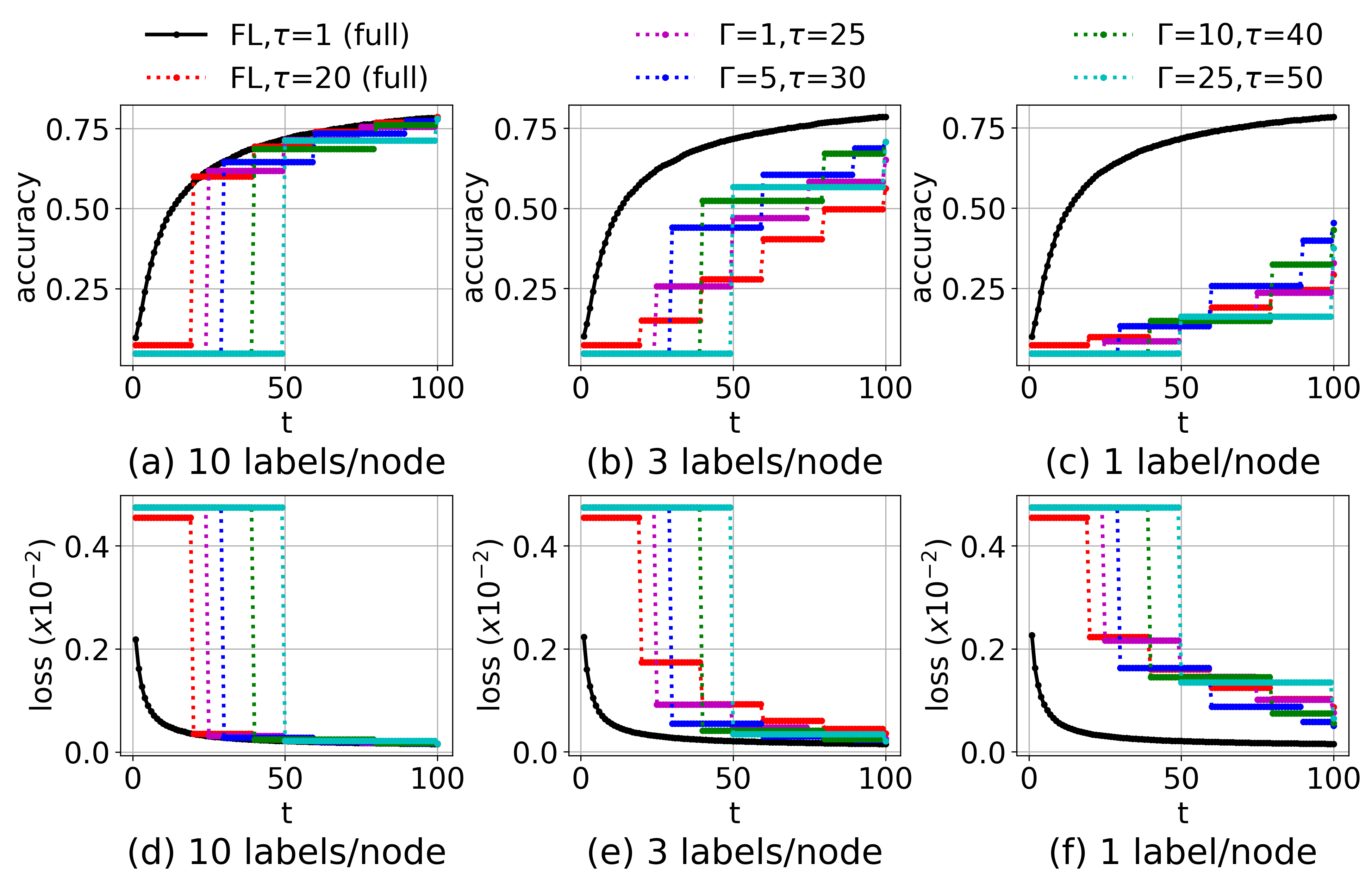
Figure 4: Performance comparison between TT-HF and baseline methods when varying the local model training interval ($\tau$) and the number of D2D consensus rounds ($\Gamma$). With a larger $\tau$, TT-HF can still outperform the baseline federated learning [16, 58] if $\Gamma$ is increased, i.e., local D2D communications can be used to offset the frequency of global aggregations. full implies that baseline schemes do not leverage D2D and instead require all the device to engage in uplink transmissions. SVM is used for classification.

$$\textrm{p}^{\mathsf{out},(t)}_{i,i^{\prime}}=1-\exp\Big{(}\frac{-(2^{R_{i,i^{\prime}}^{(t)}}-1)}{\mathrm{SNR}^{(t)}_{i,i^{\prime}}}\Big{)},$$ (39)

where $\mathrm{SNR}^{(t)}_{i,i^{\prime}}=\frac{p_{i}^{(t)}|h_{i,i^{\prime}}^{(t)}|^{2}}{\sigma^{2}}$. To construct the graph topology of each cluster $c$, we create an edge between two nodes $i$ and $i^{\prime}$ if and only if their respective outage probability satisfies $\textrm{p}^{\mathsf{out},(t)}_{i,i^{\prime}}\leq 5\%$ given a defined common data rate $R^{(t)}_{i,i^{\prime}}=R^{(t)}_{c}$, chosen as $R_{c}^{(t)}=14$ Mbps. This value is used since it is large enough to neglect the effect of quantization error in digital communication of the signals, and at the same time results in connected graphs inside the clusters (numerically, we found an average degree of 2 nodes in each cluster). After creating the topology based on the large-scale pathloss and outage probability requirements, we model outages during the consensus phase as follows: if the instantaneous channel capacity (given by (36), which captures the effect of fast fading) on an edge drops below $R_{c}^{(t)}$, outage occurs, so that the packet is lost and the model update is not received at the respective receiver. Therefore, although nodes are assumed to be static during each global aggregation period, the instantaneous cluster topology, i.e., the communication configuration among the nodes, changes with respect to every local SGD iteration in a model training interval due to outages.

Given a communication graph we choose $d_{c}=1/8$ to form the consensus iteration at each node $i$ as $\textbf{z}_{i}^{(t^{\prime}+1)}=\textbf{z}_{i}^{(t^{\prime})}+d_{{c}}\sum_{j\in\mathcal{N}_{i}}(\textbf{z}_{j}^{(t^{\prime})}-\textbf{z}_{i}^{(t^{\prime})})$ (refer to the discussion provided after Assumption 2). Note that given $d_{c}$, broadcast by the server at the beginning of each global aggregation, each node can conduct D2D communications and local averaging without any global coordination.

Datasets. We consider MNIST [61] and Fashion-MNIST (F-MNIST) [62], two datasets commonly used in image classification tasks. Each dataset contains $70$K images ($60$K for training, $10$K for testing), where each image is one of 10 labels of hand-written digits and fashion products, respectively. For brevity, we present the results for MNIST here, and refer the reader to Appendix G for FMNIST; the results are qualitatively similar.
Data distributions. To simulate varying degrees of statistical data heterogeneity among the devices, we divide the datasets into the devices’ local $\mathcal{D}_{i}$ in three ways: (a) extreme non-i.i.d., where each local dataset has only data points from a single label; (b) moderate non-i.i.d., where each local dataset contains datapoints from three of the 10 labels; and (c) i.i.d., where each local dataset has datapoints covering all $10$ labels. In each case, $\mathcal{D}_{i}$ is selected randomly (without replacement) from the full dataset of labels assigned to device $i$.

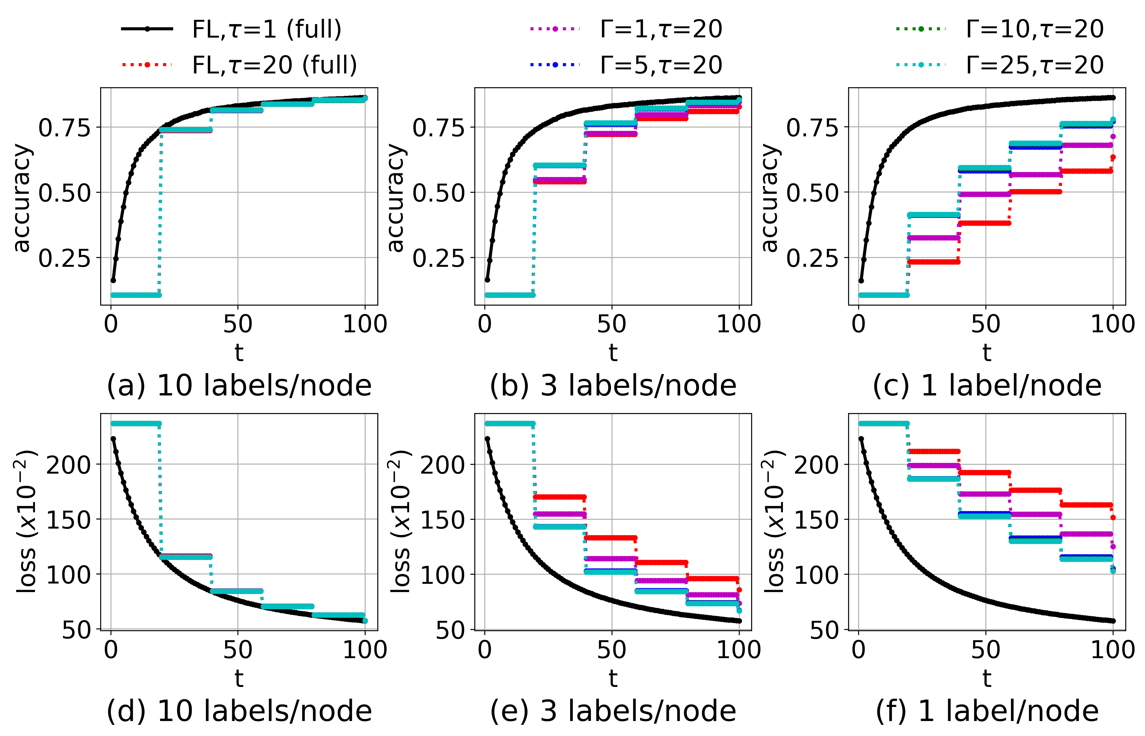
Figure 5: Performance comparison between TT-HF and baseline methods when varying the number of D2D consensus rounds ($\Gamma$). Under the same period of local model training ($\tau$), increasing $\Gamma$ results in a considerable improvement in the model accuracy/loss over time as compared to the current art [16, 58] when data is non-i.i.d. full implies that baseline schemes do not leverage D2D and instead require all the device to engage in uplink transmissions. NN is used for classification.

ML models. We consider loss functions from two different ML classifiers: regularized (squared) support vector machines (SVM) and a fully connected neural network (NN). In both cases, we use the standard implementations in PyTorch which results in a model dimension of $M=7840$ on MNIST. Note that the SVM satisfies Assumption 1, while the NN does not. The numerical results obtained for both classifiers are qualitatively similar. Thus, for brevity, we show a selection of results for each classifier here, and refer the reader to Appendix G for the extensive simulation results on both classifiers, where we also explain the implementation of our control algorithm for non-convex loss functions. The SVM uses a linear kernel, and the weights initialization follows a uniform distribution, with mean and variance calculated according to [63]. All of our implementations can be accessed at [64].

V-B TT-HF Model Training Performance and Convergence

One of the main premises of TT-HF is that cooperative consensus procedure within clusters during the local model training interval can (i) preserve model performance while reducing the required frequency of global aggregations and/or (ii) increase the model training accuracy, especially when statistical data heterogeneity is present across the devices. Our first set of experiments seek to validate these facts:

V-B1 Local consensus reducing global aggregation frequency

In Fig. 4, we compare the performance of TT-HF for increased local model training intervals $\tau$ against the current federated learning algorithms that do not exploit local D2D model consensus procedure. The baselines both assume full device participation (i.e., all devices upload their local model to the server at each global aggregation), and thus are 5x more uplink resource-intensive at each aggregation. One baseline conducts global aggregations after each round of training ($\tau=1$), and the other, based on [16], has local update intervals of $20$ ($\tau=20$). Recall that longer local training periods are desirable to reduce the frequency of communication between devices and the main server. We conduct consensus after every $t=5$ time instances, and increase $\Gamma$ as $\tau$ increases. The $\tau=1$ baseline is an upper bound on the achievable performance since it replicates centralized model training.

Fig. 4 confirms that TT-HF can still outperform the baseline FL with $\tau=20$ when the frequency of global aggregations is decreased: in other words, increasing $\tau$ can be counteracted with a higher degree of local consensus procedure $\Gamma^{(t)}_{c}=\Gamma$, $\forall c,t$. Considering the moderate non-i.i.d. plots ((b) and (e)), we also see that the jumps in global model performance, while less frequent, are substantially larger for TT-HF than the baseline. This result shows that D2D communications can reduce reliance on the main server for a more distributed model training process. It can also be noted that TT-HF achieves this performance gain despite the communication impairments, i.e., packet lost due to fast fading, that we assumed in D2D communications. This implies the robustness of TT-HF to imperfect D2D communications among the devices.

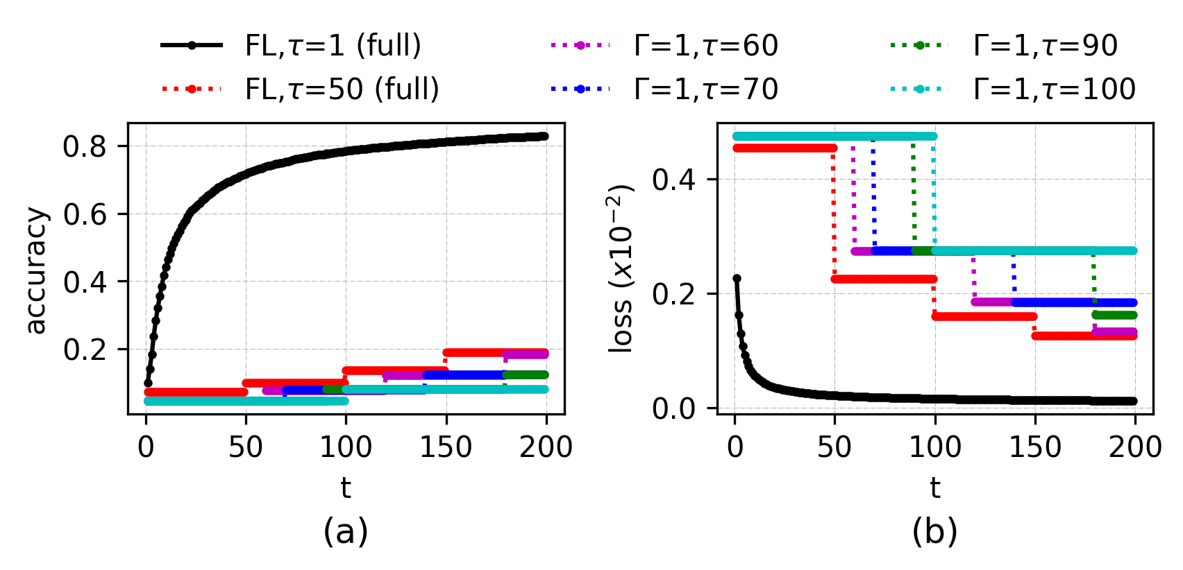
Figure 6: Performance of TT-HF in the extreme non-i.i.d. case for the setting in Fig. 4 when $\Gamma$ is small and the local model training interval length is increased substantially. TT-HF exhibits poor convergence behavior when $\tau$ exceeds a certain value, due to model dispersion. SVM is used for classification.

V-B2 D2D enhancing ML model performance

In Fig. 5, we compare the performance of TT-HF with the baseline methods, where we set $\tau_{k}=\tau=20$ and conduct a fixed number of D2D rounds in clusters after every $5$ time instances, i.e., $\Gamma^{(t)}_{c}=\Gamma$ for different values of $\Gamma$. Fig. 5 verifies that local D2D communications can significantly boost the performance of ML model training. Specifically, when the data distributions are moderate non-i.i.d ((b) and (e)) or extreme non-i.i.d. ((c) and (f)), we see that increasing $\Gamma$ improves the trained model accuracy/loss substantially from FL with $\tau=20$. It also reveals that there is a diminishing reward of increasing $\Gamma$ as the performance of TT-HF approaches that of FL with $\tau=1$. Finally, we observe that the gains obtained through D2D communications are only present when the data distributions across the nodes are non-i.i.d., as compared to the i.i.d. scenario ((a) and (d)), which emphasizes the purpose of TT-HF for handling statistical heterogeneity. This result further shows the applicability of TT-HF to non-convex classifiers such as NN.

V-B3 Convergence behavior

Recall that the upper bound on convergence in Theorem 1 is dependent on the expected model dispersion $A^{(t)}$ and the consensus error $\epsilon^{(t)}$ across clusters. For the settings in Figs. 5&4, increasing the local model training period $\tau$ and decreasing the consensus rounds $\Gamma$ will result in increased $A^{(t)}$ and $\epsilon^{(t)}$, respectively, for a given $t$. In Fig. 6, we show that TT-HF suffers from poor convergence behavior in the extreme non-i.i.d. case when the period of local descents $\tau$ are excessively prolonged, similar to the baseline FL when $\tau=50$ [16]. This further emphasizes the importance of Algorithm 2 tuning these parameters around Theorem 2’s result.

V-C TT-HF with Adaptive Parameter Control

We turn now to evaluating the efficacy and analyzing the behavior of TT-HF under parameter tuning from Algorithm 2.

V-C1 Improved resource efficiency compared with baselines

Fig. 7 compares the performance of TT-HF under our control algorithm with the two baselines: (i) FL with full device participation and $\tau=1$ (from Sec. V-B), and (ii) FL with $\tau=20$ but only one device sampled from each cluster for global aggregations. The result is shown under different ratios of delays $\frac{\Delta_{\textrm{D2D}}}{\Delta_{\textrm{Glob}}}$ and different ratios of energy consumption $\frac{E_{\textrm{D2D}}}{E_{\textrm{Glob}}}$ between D2D communications and global aggregations. Three metrics are shown: (a) total cost based on the objective of $(\bm{\mathcal{P}})$, (b) total energy consumed, and (c) total delay experienced up to the point where $75\%$ of peak accuracy is reached.

Overall, in (a), we see that TT-HF (depicted through the bars) outperforms the baselines (depicted through the horizontal lines) substantially in terms of total cost, by at least 75% in each case. In (b), we observe that for smaller values of ${E_{\textrm{D2D}}}/{E_{\textrm{Glob}}}$, TT-HF lowers the overall power consumption, but after the D2D energy consumption reaches a certain threshold, it does not result in energy savings anymore. The same impact can be observed regarding the delay from (c), i.e., once $\frac{\Delta_{\textrm{D2D}}}{\Delta_{\textrm{Glob}}}\approx 0.1$ there is no longer an advantage in terms of delay. Ratios of $0.1$ for either of these metrics, however, is significantly larger than what is being observed in 5G networks [51, 52], indicating that TT-HF would be effective in practical systems.

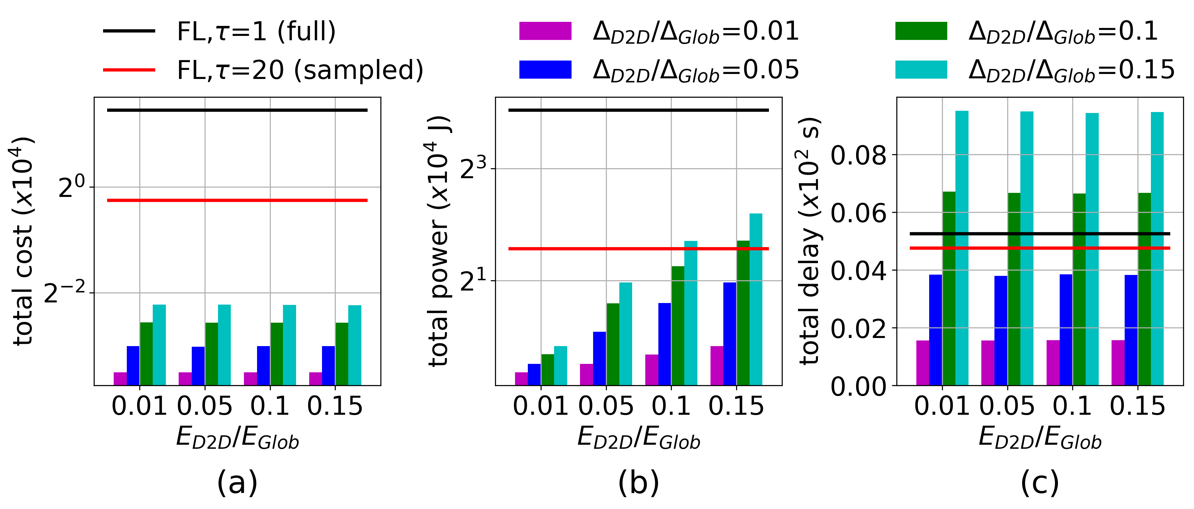
Figure 7: Comparing total (a) cost, (b) power, and (c) delay metrics from the optimization objective in $(\bm{\mathcal{P}})$ achieved by TT-HF versus baselines upon reaching $75\%$ of peak accuracy, for different configurations of delay and energy consumption. TT-HF obtains a significantly lower total cost in (a). (b) and (c) demonstrate the region under which TT-HF attains energy savings and delay gains. SVM is used for classification.

V-C2 Impact of design choices on local model training interval

We are also interested in how the design weights $c_{1},c_{2},c_{3}$ in $(\bm{\mathcal{P}})$ affect the behavior of the control algorithm. In Fig. 8, we plot the value of $\tau_{2}$, i.e., the length of the second local model training interval, for different configurations of $c_{1}$, $c_{2}$ and $c_{3}$. The maximum tolerable value of $\tau$ is assumed to be $40$. As we can see, increasing $c_{1}$ and $c_{2}$ – which elevates the priority on minimizing energy consumption and delay, respectively – results in a longer local model training interval, since D2D communication is more efficient. On the other hand, increasing $c_{3}$ – which prioritizes the global model convergence rate – results in a quicker global aggregation.

V-D Main Takeaways

Data heterogeneity in local dataset across local devices can result in considerable performance degradation of federated learning algorithms. In this case, longer local update periods will result in models that are significantly biased towards local datasets and degrade the convergence speed of the global model and the resulting model accuracy. By blending federated aggregations with cooperative D2D consensus procedure among local device clusters in TT-HF, we effectively decrease the bias of the local models to the local datasets and speed up the convergence at a lower cost (i.e., utilizing low power D2D communications to reduce the frequency of performing global aggregation via uplink transmissions). Due to the low network cost in performing D2D transmission, TT-HF provides a practical solution for federated learning to achieve faster convergence or to prolong the local model training interval, leading to delay and energy consumption savings.

Although we develop our algorithm based on federated learning with vanilla SGD local optimizer, our method can benefit other counterparts in the literature. This is due to the fact that, intuitively, conducting D2D communications via the method proposed on this paper reduces the local bias of the nodes’ models to their local datasets, which is one of the main challenges faced in federated learning. In Appendix G we conduct some preliminary experiment to show the impact of our method on FedProx [65].

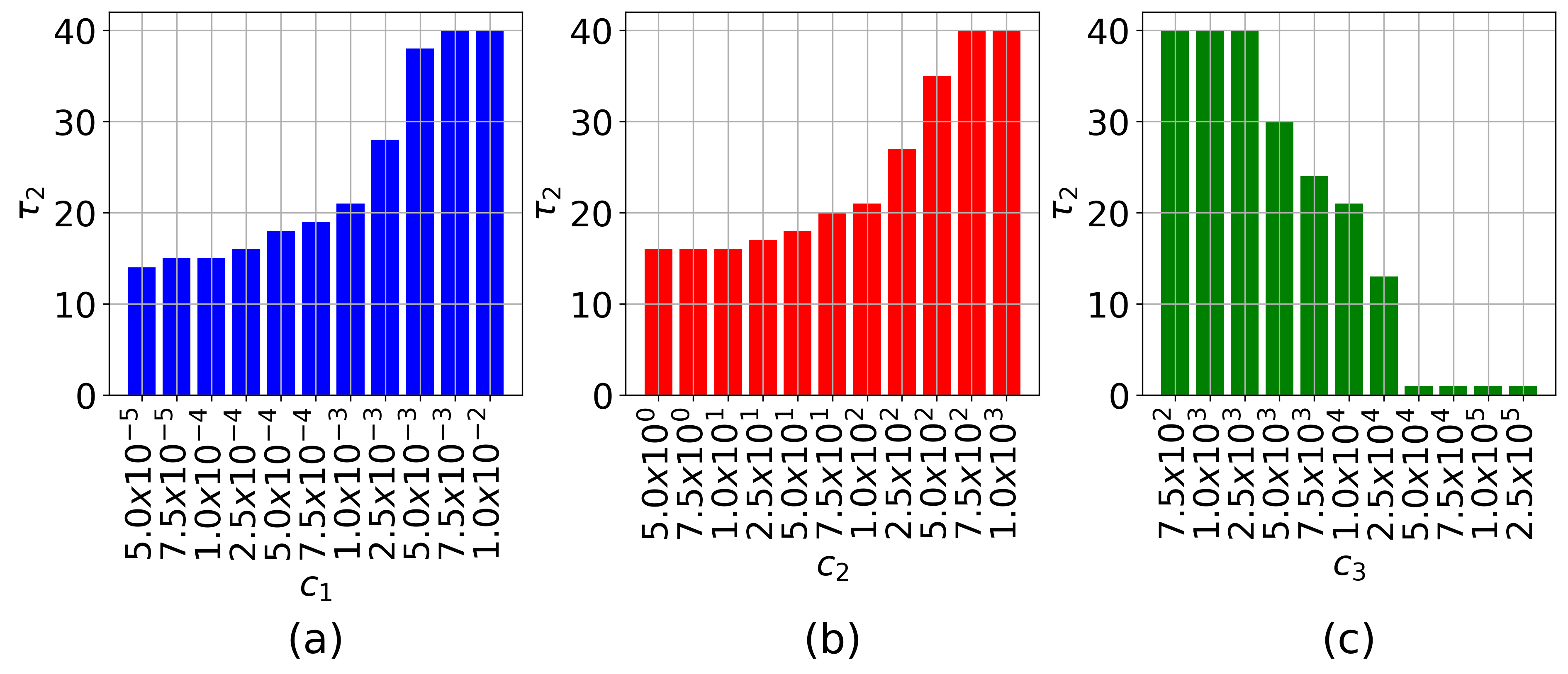
Figure 8: Value of the second local model training interval obtained through $(\bm{\mathcal{P}})$ for different configurations of weighing coefficients $c_{1},c_{2},c_{3}$ (default $c_{1}=10^{-3},c_{2}=10^{2},c_{3}=10^{4}$). Higher weight on energy and delay (larger $c_{1}$ and $c_{2}$) prolongs the local training period, while higher weight on the global model loss (larger $c_{3}$) decreases the length, resulting in more rapid global aggregations.

VI Conclusion and Future Work

We proposed TT-HF, a methodology which improves the efficiency of federated learning in D2D-enabled wireless networks by augmenting global aggregations with cooperative consensus procedure among device clusters. We conducted a formal convergence analysis of TT-HF, resulting in a bound which quantifies the impact of gradient diversity, consensus error, and global aggregation periods on the convergence behavior. Using this bound, we characterized a set of conditions under which TT-HF is guaranteed to converge sublinearly with rate of $\mathcal{O}(1/t)$. Based on these conditions, we developed an adaptive control algorithm that actively tunes the device learning rate, cluster consensus rounds, and global aggregation periods throughout the training process. Our experimental results demonstrated the robustness of TT-HF against data heterogeneity among edge devices, and its improvement in trained model accuracy, training time, and/or network resource utilization in different scenarios compared to the current art.

There are several avenues for future work. To further enhance the flexibility of TT-HF, one may consider (i) heterogeneity in computation capabilities across edge devices, (ii) different communication delays from the clusters to the server, and (iii) wireless interference caused by D2D communications. Furthermore, using the set of new techniques we provided to conduct convergence analysis in this paper, we aim to extend our convergence analysis to non-convex settings in future work. This includes obtaining the conditions under which approaching a stationary point of the global loss function is guaranteed, and the rate under which the convergence is achieved.

Preliminaries and Notations used in the Proofs

In the following Appendices, in order to increase the tractability of the the expressions inside the proofs, we introduce the the following scaled parameters: (i) strong convexity denoted by $\tilde{\mu}$, normalized gradient diversity by $\tilde{\delta}$, step size by $\tilde{\eta_{t}}$, SGD variance $\tilde{\sigma}$, and consensus error inside the clusters $\tilde{\epsilon}_{c}^{(t)}$ and across the network $\tilde{\epsilon}^{(t)}$ inside the cluster as follows:

• Strong convexity: $F$ is $\mu$-strongly convex, i.e.,

  $$F(\mathbf{w}_{1})\geq F(\mathbf{w}_{2}) +\nabla F(\mathbf{w}_{2})^{\top}(\mathbf{w}_{1}-\mathbf{w}_{2})+\frac{\tilde{\mu}\beta}{2}\Big{\|}\mathbf{w}_{1}-\mathbf{w}_{2}\Big{\|}^{2},\leavevmode\nobreak\ \forall{\mathbf{w}_{1},\mathbf{w}_{2}},$$ (40)

  where as compared to Assumption 1, we considered $\tilde{\mu}=\mu/\beta\in(0,1)$.

• Gradient diversity: The gradient diversity across the device clusters $c$ is measured via two non-negative constants $\delta,\zeta$ that satisfy

  $$\|\nabla\hat{F}_{c}(\mathbf{w})-\nabla F(\mathbf{w})\|\leq\sqrt{\beta}\tilde{\delta}+2\omega\beta\|\mathbf{w}-\mathbf{w}^{*}\|,\leavevmode\nobreak\ \forall c,\mathbf{w},$$ (41)

  where as compared to Assumption 1, we presumed $\tilde{\delta}=\delta/\sqrt{\beta}$ and $\omega=\zeta/(2\beta)\in[0,1]$.

• Step size: The local updates to compute intermediate updated local model at the devices is expressed as follows:

  $${\widetilde{\mathbf{w}}}_{i}^{(t)}=\mathbf{w}_{i}^{(t-1)}-\frac{\tilde{\eta}_{t-1}}{\beta}\widehat{\mathbf{g}}_{i}^{(t-1)},\leavevmode\nobreak\ t\in\mathcal{T}_{k},$$ (42)

  where we used the scaled in the step size, i.e., ${\tilde{\eta}_{t-1}}=\eta_{t-1}{\beta}$. Also, when we consider decreasing step size, we consider scaled parameter $\tilde{\gamma}$ in the step size as follows: $\frac{\gamma}{t+\alpha}=\frac{\tilde{\gamma}/\beta}{t+\alpha}$ indicating that $\tilde{\gamma}=\gamma\beta$.

• Variance of the noise of the estimated gradient through SGD: The variance on the SGD noise is bounded as:

  $$\mathbb{E}[\|{\mathbf{n}}_{j}^{(t)}\|^{2}]\leq\beta\tilde{\sigma}^{2},\forall j,t,$$ (43)

  where we consider scaled SGD noise as: $\tilde{\sigma}^{2}=\sigma^{2}/\beta$.

• Average of the consensus error inside cluster $c$ and across the network: $\epsilon_{c}^{(t)}$ is an upper bound on the average of the consensus error inside cluster $c$ for time $t$, i.e.,

  $$\frac{1}{s_{c}}\sum\limits_{i\in\mathcal{S}_{c}}\|\mathbf{e}_{i}^{(t)}\|^{2}\leq(\tilde{\epsilon}_{c}^{(t)})^{2}/\beta,$$ (44)

  where we use the scaled consensus error $(\tilde{\epsilon}_{c}^{(t)})^{2}=\beta(\epsilon_{c}^{(t)})^{2}$. Also, in the proofs we use the notation $\epsilon$ to denote the average consensus error across the network defined as $(\epsilon^{(t)})^{2}=\sum_{c=1}^{N}\varrho_{c}(\epsilon_{c}^{(t)})^{2}$. When the consensus is assumed to be decreasing over time we use the scaled coefficient $\tilde{\phi}^{2}=\phi^{2}/\beta$, resulting in $(\epsilon^{(t)})^{2}=\eta_{t}^{2}\tilde{\phi}^{2}\beta$.

Finally, to track the global model variations, we introduce the instantaneous global model $\hat{\mathbf{w}}^{(t)}=\sum\limits_{c=1}^{N}\varrho_{c}\mathbf{w}_{n_{c}}^{(t)}$, where $n_{c}$ is a node uniformly sampled from cluster $c$. We note that $\hat{\mathbf{w}}^{(t)}$ is only realized at the server at the instance of the global aggregations.

Appendix A Proof of Proposition 1

Proposition 1.

Under Assumptions 1 and 3, if $\eta_{t}=\frac{\gamma}{t+\alpha}$, $\epsilon^{(t)}$ is non-increasing with respect to $t\in\mathcal{T}_{k}$, i.e., $\epsilon^{(t+1)}/\epsilon^{(t)}\leq 1$ and $\alpha\geq\max\{\beta\gamma[\frac{\mu}{4\beta}-1+\sqrt{(1+\frac{\mu}{4\beta})^{2}+2\omega}],\frac{\beta^{2}\gamma}{\mu}\}$, using TT-HF for ML model training, the following upper bound on the expected model dispersion across the clusters holds:

$$A^{(t)}\leq\frac{16\omega^{2}}{\mu}[\Sigma_{+,t}]^{2}[F(\bar{\mathbf{w}}(t_{k-1}))-F(\mathbf{w}^{*})]+25[\Sigma_{+,t}]^{2}\left[\frac{\sigma^{2}}{\beta^{2}}+\frac{\delta^{2}}{\beta^{2}}+(\epsilon^{(0)})^{2}\right],\leavevmode\nobreak\ \leavevmode\nobreak\ t\in\mathcal{T}_{k},$$ (45)

where

$$[\Sigma_{+,t}]^{2}=\left[\sum\limits_{\ell=t_{k-1}}^{t-1}\left(\prod_{j=t_{k-1}}^{\ell-1}(1+\eta_{j}\beta\lambda_{+})\right)\beta\eta_{\ell}\left(\prod_{j=\ell+1}^{t-1}(1+\eta_{j}\beta)\right)\right]^{2},$$ (46)

and

$$\lambda_{+}=1-\frac{\mu}{4\beta}+\sqrt{(1+\frac{\mu}{4\beta})^{2}+2\omega}.$$ (47)

Proof.

We break down the proof into 3 parts: in Part I we find the relationship between $\|\bar{\mathbf{w}}^{(t)}-\mathbf{w}^{*}\|$ and $\sum\limits_{c=1}^{N}\varrho_{c}\|\bar{\mathbf{w}}_{c}^{(t)}-\bar{\mathbf{w}}^{(t)}\|$, which turns out to form a coupled dynamic system, which is solved in Part II. Finally, Part III draws the connection between $A^{(t)}$ and the solution of the coupled dynamic system and obtains the upper bound on $A^{(t)}$.

(Part I) Finding the relationship between $\|\bar{\mathbf{w}}^{(t)}-\mathbf{w}^{*}\|$ and $\sum\limits_{c=1}^{N}\varrho_{c}\|\bar{\mathbf{w}}_{c}^{(t)}-\bar{\mathbf{w}}^{(t)}\|$: Using the definition of $\bar{\mathbf{w}}^{(t+1)}$ given in Definition 2, and the notations introduced in Appendix Preliminaries and Notations used in the Proofs, we have:

$$\bar{\mathbf{w}}^{(t+1)}=\bar{\mathbf{w}}^{(t)}-\frac{\tilde{\eta_{t}}}{\beta}\sum\limits_{c=1}^{N}\varrho_{c}\frac{1}{s_{c}}\sum\limits_{j\in\mathcal{S}_{c}}\widehat{\mathbf{g}}_{j,t},\leavevmode\nobreak\ t\in\mathcal{T}_{k}.$$ (48)

Adding and subtracting terms in the above equality gives us:

$$\bar{\mathbf{w}}^{(t+1)}-\mathbf{w}^{*}= \leavevmode\nobreak\ \bar{\mathbf{w}}^{(t)}-\mathbf{w}^{*}-\frac{\tilde{\eta_{t}}}{\beta}\nabla F(\bar{\mathbf{w}}^{(t)})$$

$$-\frac{\tilde{\eta_{t}}}{\beta}\sum\limits_{c=1}^{N}\varrho_{c}\frac{1}{s_{c}}\sum\limits_{j\in\mathcal{S}_{c}}[\widehat{\mathbf{g}}_{j,t}-\nabla F_{j}(\mathbf{w}_{j}^{(t)})]$$

$$-\frac{\tilde{\eta_{t}}}{\beta}\sum\limits_{c=1}^{N}\varrho_{c}\frac{1}{s_{c}}\sum\limits_{j\in\mathcal{S}_{c}}[\nabla F_{j}(\mathbf{w}_{j}^{(t)})-\nabla F_{j}(\bar{\mathbf{w}}_{c}^{(t)})]$$

$$-\frac{\tilde{\eta_{t}}}{\beta}\sum\limits_{c=1}^{N}\varrho_{c}[\nabla F_{c}(\bar{\mathbf{w}}_{c}^{(t)})-\nabla F_{c}(\bar{\mathbf{w}}^{(t)})].$$ (49)

Taking the norm-2 from the both hand sides of the above equality and applying the triangle inequality yields:

$$\|\bar{\mathbf{w}}^{(t+1)}-\mathbf{w}^{*}\|\leq \|\bar{\mathbf{w}}^{(t)}-\mathbf{w}^{*}-\frac{\tilde{\eta_{t}}}{\beta}\nabla F(\bar{\mathbf{w}}^{(t)})\|+\frac{\tilde{\eta_{t}}}{\beta}\sum\limits_{c=1}^{N}\varrho_{c}\frac{1}{s_{c}}\sum\limits_{j\in\mathcal{S}_{c}}\|\mathbf{n}_{j}^{(t)}\|$$

$$+\frac{\tilde{\eta_{t}}}{\beta}\sum\limits_{c=1}^{N}\varrho_{c}\frac{1}{s_{c}}\sum\limits_{j\in\mathcal{S}_{c}}\|\nabla F_{j}(\mathbf{w}_{j}^{(t)})-\nabla F_{j}(\bar{\mathbf{w}}_{c}^{(t)})\|$$

$$+\frac{\tilde{\eta_{t}}}{\beta}\sum\limits_{c=1}^{N}\varrho_{c}\|\nabla F_{c}(\bar{\mathbf{w}}_{c}^{(t)})-\nabla F_{c}(\bar{\mathbf{w}}^{(t)})\|.$$ (50)

To bound the terms on the right hand side above, we first use the $\mu$-strong convexity and $\beta$-smoothness of $F(\cdot)$, when $\eta_{t}\leq\frac{\mu}{\beta^{2}}$, to get

$$\|\bar{\mathbf{w}}^{(t)}-\mathbf{w}^{*}-\frac{\tilde{\eta_{t}}}{\beta}\nabla F(\bar{\mathbf{w}}^{(t)})\|$$

$$=\sqrt{\|\bar{\mathbf{w}}^{(t)}-\mathbf{w}^{*}\|^{2}+(\frac{\tilde{\eta_{t}}}{\beta})^{2}\|\nabla F(\bar{\mathbf{w}}^{(t)})\|^{2}-\frac{2\tilde{\eta_{t}}}{\beta}(\bar{\mathbf{w}}^{(t)}-\mathbf{w}^{*})^{\top}\nabla F(\bar{\mathbf{w}}^{(t)})}$$

$$\overset{(a)}{\leq}\sqrt{(1-2\tilde{\eta}_{t}\tilde{\mu})\|\bar{\mathbf{w}}^{(t)}-\mathbf{w}^{*}\|^{2}+(\frac{\tilde{\eta_{t}}}{\beta})^{2}\|\nabla F(\bar{\mathbf{w}}^{(t)})\|^{2}}$$

$$\overset{(b)}{\leq}\sqrt{1-2\tilde{\eta}_{t}\tilde{\mu}+\tilde{\eta}_{t}^{2}}\|\bar{\mathbf{w}}^{(t)}-\mathbf{w}^{*}\|\overset{(c)}{\leq}(1-\frac{\tilde{\eta}_{t}\tilde{\mu}}{2})\|\bar{\mathbf{w}}^{(t)}-\mathbf{w}^{*}\|,$$ (51)

where $(a)$ results from the property of a strongly convex function, i.e., $(\bar{\mathbf{w}}^{(t)}-\mathbf{w}^{*})^{\top}\nabla F(\bar{\mathbf{w}}^{(t)})\geq\tilde{\mu}\beta\|\bar{\mathbf{w}}^{(t)}-\mathbf{w}^{*}\|^{2}$, $(b)$ comes from the property of smooth functions, i.e., $\|\nabla F(\bar{\mathbf{w}}^{(t)})\|^{2}\leq\beta^{2}\|\bar{\mathbf{w}}^{(t)}-\mathbf{w}^{*}\|^{2}$ and the last step $(c)$ follows from the fact that $\tilde{\eta}_{t}\leq\tilde{\eta}_{0}$ and assuming $\tilde{\eta}_{0}\leq\tilde{\mu}$, implying $\alpha\geq\tilde{\gamma}/\tilde{\mu}$. Also, considering the other terms on the right hand side of (A), using $\beta$-smoothness, we have

$$\|\nabla F_{j}(\mathbf{w}_{j}^{(t)})-\nabla F_{j}(\bar{\mathbf{w}}_{c}^{(t)})\|\leq\beta\frac{1}{s_{c}}\sum\limits_{j\in\mathcal{S}_{c}}\|\mathbf{w}_{j}^{(t)}-\bar{\mathbf{w}}_{c}^{(t)}\|.$$ (52)

Moreover, using Condition 1, we get

$$\frac{1}{s_{c}}\sum\limits_{j\in\mathcal{S}_{c}}\|\mathbf{w}_{j}^{(t)}-\bar{\mathbf{w}}_{c}^{(t)}\| =\frac{1}{s_{c}}\sum\limits_{j\in\mathcal{S}_{c}}\|\mathbf{e}_{j}^{(t)}\|$$

$$\leq\sqrt{\frac{1}{s_{c}}\sum\limits_{j\in\mathcal{S}_{c}}\|\mathbf{e}_{j}^{(t)}\|^{2}}\leq\tilde{\epsilon}_{c}^{(t)}/\sqrt{\beta}.$$ (53)

Combining (52) and (A) gives us:

$$\frac{1}{s_{c}}\sum\limits_{j\in\mathcal{S}_{c}}\|\nabla F_{j}(\mathbf{w}_{j}^{(t)})-\nabla F_{j}(\bar{\mathbf{w}}_{c}^{(t)})\|\leq\sqrt{\beta}\tilde{\epsilon}_{c}^{(t)}.$$ (54)

Replacing the result of (A) and (54) in (A) yields:

$$\|\bar{\mathbf{w}}^{(t+1)}-\mathbf{w}^{*}\|\leq (1-\frac{\tilde{\eta}_{t}\tilde{\mu}}{2})\|\bar{\mathbf{w}}^{(t)}-\mathbf{w}^{*}\|+\frac{\tilde{\eta}_{t}}{\beta}\sum\limits_{c=1}^{N}\varrho_{c}\frac{1}{s_{c}}\sum\limits_{j\in\mathcal{S}_{c}}\|\mathbf{n}_{j}^{(t)}\|$$

$$+\frac{\tilde{\eta}_{t}}{\sqrt{\beta}}\sum\limits_{c=1}^{N}\varrho_{c}\tilde{\epsilon}_{c}^{(t)}+\tilde{\eta}_{t}\sum\limits_{c=1}^{N}\varrho_{c}\|\bar{\mathbf{w}}_{c}^{(t)}-\bar{\mathbf{w}}^{(t)}\|.$$ (55)

Multiplying the both hand sides of the above inequality by $\sqrt{\beta}$ followed by taking square and expectation, we get

$$\mathbb{E}\left[\sqrt{\beta}\|\bar{\mathbf{w}}^{(t+1)}-\mathbf{w}^{*}\|\right]^{2}\leq \mathbb{E}\bigg{[}\sqrt{\beta}(1-\frac{\tilde{\eta}_{t}\tilde{\mu}}{2})\|\bar{\mathbf{w}}^{(t)}-\mathbf{w}^{*}\|+\frac{\tilde{\eta}_{t}}{\sqrt{\beta}}\sum\limits_{c=1}^{N}\varrho_{c}\frac{1}{s_{c}}\sum\limits_{j\in\mathcal{S}_{c}}\|\mathbf{n}_{j}^{(t)}\|$$

$$+{\tilde{\eta}_{t}}\sum\limits_{c=1}^{N}\varrho_{c}\tilde{\epsilon}_{c}^{(t)}+\tilde{\eta}_{t}\sqrt{\beta}\sum\limits_{c=1}^{N}\varrho_{c}\|\bar{\mathbf{w}}_{c}^{(t)}-\bar{\mathbf{w}}^{(t)}\|\bigg{]}^{2}.$$ (56)

Taking the square roots from the both hand sides and using Fact 1 (See Appendix F) yields:

$$\sqrt{\beta\mathbb{E}[\|\bar{\mathbf{w}}^{(t+1)}-\mathbf{w}^{*}\|^{2}]}\leq (1-\frac{\tilde{\eta}_{t}\tilde{\mu}}{2})\sqrt{\beta\mathbb{E}[\|\bar{\mathbf{w}}^{(t)}-\mathbf{w}^{*}\|^{2}]}+{\tilde{\eta}_{t}}\tilde{\sigma}$$

$$+{\tilde{\eta}_{t}}\sum\limits_{c=1}^{N}\varrho_{c}\tilde{\epsilon}_{c}^{(t)}+\tilde{\eta}_{t}\sqrt{\beta\Big{(}\sum\limits_{c=1}^{N}\varrho_{c}\mathbb{E}\|\bar{\mathbf{w}}_{c}^{(t)}-\bar{\mathbf{w}}^{(t)}\|\Big{)}^{2}}.$$ (57)

We compact (A) and represent it via the following relationship:

$$x_{2}^{(t+1)}\leq\begin{bmatrix}\tilde{\eta}_{t}&(1-\frac{\tilde{\eta}_{t}\tilde{\mu}}{2})\end{bmatrix}\mathbf{x}^{(t)}+\tilde{\eta}_{t}\left(\tilde{\sigma}+\sum\limits_{c=1}^{N}\varrho_{c}\tilde{\epsilon}_{c}^{(t)}\right),$$ (58)

where $\mathbf{x}^{(t)}=\begin{bmatrix}x_{1}^{(t)}&x_{2}^{(t)}\end{bmatrix}^{\top}$, $x_{1}^{(t)}=\sqrt{\beta\mathbb{E}[(\sum\limits_{c=1}^{N}\varrho_{c}\|\bar{\mathbf{w}}_{c}^{(t)}-\bar{\mathbf{w}}^{(t)}\|)^{2}]}$, and $x_{2}^{(t)}=\sqrt{\beta\mathbb{E}[\|\bar{\mathbf{w}}^{(t)}-\mathbf{w}^{*}\|^{2}]}$.

The relationship in (58) reveals the dependency of $x_{2}^{(t+1)}$ on $x_{2}^{(t)}$ and $x_{1}^{(t)}$. To bound $x^{(t)}_{1}$, we first use the fact that $\bar{\mathbf{w}}_{c}^{(t+1)}$ can be written as follows:

$$\bar{\mathbf{w}}_{c}^{(t+1)}=\bar{\mathbf{w}}_{c}^{(t)}-\frac{\tilde{\eta}_{t}}{\beta}\frac{1}{s_{c}}\sum\limits_{j\in\mathcal{S}_{c}}\nabla F_{j}(\mathbf{w}_{j}^{(t)})-\frac{\tilde{\eta}_{t}}{\beta}\frac{1}{s_{c}}\sum\limits_{j\in\mathcal{S}_{c}}\mathbf{n}_{j}^{(t)}.$$ (59)

Similarly, $\bar{\mathbf{w}}^{(t+1)}$ can be written as:

$$\bar{\mathbf{w}}^{(t+1)}=\bar{\mathbf{w}}^{(t)}-\frac{\tilde{\eta}_{t}}{\beta}\sum\limits_{d=1}^{N}\varrho_{d}\frac{1}{s_{d}}\sum\limits_{j\in\mathcal{S}_{d}}\nabla F_{j}(\mathbf{w}_{j}^{(t)})-\frac{\tilde{\eta}_{t}}{\beta}\sum\limits_{d=1}^{N}\varrho_{d}\frac{1}{s_{d}}\sum\limits_{j\in\mathcal{S}_{d}}\mathbf{n}_{j}^{(t)}.$$ (60)

Combining (59) and (60) and performing some algebraic manipulations yields:

$$\bar{\mathbf{w}}_{c}^{(t+1)}-\bar{\mathbf{w}}^{(t+1)}=\bar{\mathbf{w}}_{c}^{(t)}-\bar{\mathbf{w}}^{(t)}-\frac{\tilde{\eta}_{t}}{\beta}\frac{1}{s_{c}}\sum\limits_{j\in\mathcal{S}_{c}}\mathbf{n}_{j}^{(t)}+\frac{\tilde{\eta}_{t}}{\beta}\sum\limits_{d=1}^{N}\varrho_{d}\frac{1}{s_{d}}\sum\limits_{j\in\mathcal{S}_{d}}\mathbf{n}_{j}^{(t)}$$

$$-\frac{\tilde{\eta}_{t}}{\beta}\frac{1}{s_{c}}\sum\limits_{j\in\mathcal{S}_{c}}\Big{[}\nabla F_{j}(\bar{\mathbf{w}}_{j}^{(t)})-\nabla F_{j}(\bar{\mathbf{w}}_{c}^{(t)})\Big{]}+\frac{\tilde{\eta}_{t}}{\beta}\sum\limits_{d=1}^{N}\varrho_{d}\frac{1}{s_{d}}\sum\limits_{j\in\mathcal{S}_{d}}\Big{[}\nabla F_{j}(\bar{\mathbf{w}}_{j}^{(t)})-\nabla F_{j}(\bar{\mathbf{w}}_{d}^{(t)})\Big{]}$$

$$-\frac{\tilde{\eta}_{t}}{\beta}\Big{[}\nabla\hat{F}_{c}(\bar{\mathbf{w}}_{c}^{(t)})-\nabla\hat{F}_{c}(\bar{\mathbf{w}}^{(t)})\Big{]}+\frac{\tilde{\eta}_{t}}{\beta}\sum\limits_{d=1}^{N}\varrho_{d}\Big{[}\nabla\hat{F}_{d}(\bar{\mathbf{w}}_{d}^{(t)})-\nabla\hat{F}_{d}(\bar{\mathbf{w}}^{(t)})\Big{]}$$

$$-\frac{\tilde{\eta}_{t}}{\beta}\Big{[}\nabla\hat{F}_{c}(\bar{\mathbf{w}}^{(t)})-\nabla F(\bar{\mathbf{w}}^{(t)})\Big{]}.$$ (61)

Taking the norm-2 of the both hand sides of the above equality and applying the triangle inequality gives us

$$\|\bar{\mathbf{w}}_{c}^{(t+1)}-\bar{\mathbf{w}}^{(t+1)}\|\leq\|\bar{\mathbf{w}}_{c}^{(t)}-\bar{\mathbf{w}}^{(t)}\|+\frac{\tilde{\eta}_{t}}{\beta}\|\frac{1}{s_{c}}\sum\limits_{j\in\mathcal{S}_{c}}\mathbf{n}_{j}^{(t)}\|+\frac{\tilde{\eta}_{t}}{\beta}\|\sum\limits_{d=1}^{N}\varrho_{d}\frac{1}{s_{d}}\sum\limits_{j\in\mathcal{S}_{d}}\mathbf{n}_{j}^{(t)}\|$$

$$+\frac{\tilde{\eta}_{t}}{\beta}\frac{1}{s_{c}}\sum\limits_{j\in\mathcal{S}_{c}}\|\nabla F_{j}(\bar{\mathbf{w}}_{j}^{(t)})-\nabla F_{j}(\bar{\mathbf{w}}_{c}^{(t)})\|+\frac{\tilde{\eta}_{t}}{\beta}\sum\limits_{d=1}^{N}\varrho_{d}\frac{1}{s_{d}}\sum\limits_{j\in\mathcal{S}_{d}}\|\nabla F_{j}(\bar{\mathbf{w}}_{j}^{(t)})-\nabla F_{j}(\bar{\mathbf{w}}_{d}^{(t)})\|$$

$$+\frac{\tilde{\eta}_{t}}{\beta}\|\nabla\hat{F}_{c}(\bar{\mathbf{w}}_{c}^{(t)})-\nabla\hat{F}_{c}(\bar{\mathbf{w}}^{(t)})\|+\frac{\tilde{\eta}_{t}}{\beta}\sum\limits_{d=1}^{N}\varrho_{d}\|\nabla\hat{F}_{d}(\bar{\mathbf{w}}_{d}^{(t)})-\nabla\hat{F}_{d}(\bar{\mathbf{w}}^{(t)})\|$$

$$+\frac{\tilde{\eta}_{t}}{\beta}\|\nabla\hat{F}_{c}(\bar{\mathbf{w}}^{(t)})-\nabla F(\bar{\mathbf{w}}^{(t)})\|.$$ (62)

Using $\beta$-smoothness of $F_{j}(\cdot)$, $\forall j$, and $\hat{F}_{c}(\cdot)$, $\forall c$, Definition 1 and Condition 1, we further bound the right hand side of (A) to get

$$\|\bar{\mathbf{w}}_{c}^{(t+1)}-\bar{\mathbf{w}}^{(t+1)}\|\leq(1+\tilde{\eta}_{t})\|\bar{\mathbf{w}}_{c}^{(t)}-\bar{\mathbf{w}}^{(t)}\|+2\omega\tilde{\eta}_{t}\|\bar{\mathbf{w}}^{(t)}-\mathbf{w}^{*}\|+\tilde{\eta}_{t}\sum\limits_{d=1}^{N}\varrho_{d}\|\bar{\mathbf{w}}_{d}^{(t)}-\bar{\mathbf{w}}^{(t)}\|$$

$$+\frac{\tilde{\eta}_{t}}{\beta}\|\frac{1}{s_{c}}\sum\limits_{j\in\mathcal{S}_{c}}\mathbf{n}_{j}^{(t)}\|+\frac{\tilde{\eta}_{t}}{\beta}\|\sum\limits_{d=1}^{N}\varrho_{d}\frac{1}{s_{d}}\sum\limits_{j\in\mathcal{S}_{d}}\mathbf{n}_{j}^{(t)}\|$$

$$+\tilde{\eta}_{t}\frac{1}{s_{c}}\sum\limits_{j\in\mathcal{S}_{c}}\|\bar{\mathbf{w}}_{j}^{(t)}-\bar{\mathbf{w}}_{c}^{(t)}\|+\tilde{\eta}_{t}\sum\limits_{d=1}^{N}\varrho_{d}\frac{1}{s_{d}}\sum\limits_{j\in\mathcal{S}_{d}}\|\bar{\mathbf{w}}_{j}^{(t)}-\bar{\mathbf{w}}_{d}^{(t)}\|+\frac{\tilde{\eta}_{t}}{\sqrt{\beta}}\tilde{\delta}.$$ (63)

Using (A) we have $\frac{1}{s_{d}}\sum\limits_{j\in\mathcal{S}_{d}}\|\bar{\mathbf{w}}_{j}^{(t)}-\bar{\mathbf{w}}_{d}^{(t)}\|\leq\frac{\tilde{\epsilon}_{d}^{(t)}}{\sqrt{\beta}}$, and thus (A) can be written as

$$\|\bar{\mathbf{w}}_{c}^{(t+1)}-\bar{\mathbf{w}}^{(t+1)}\|\leq(1+\tilde{\eta}_{t})\|\bar{\mathbf{w}}_{c}^{(t)}-\bar{\mathbf{w}}^{(t)}\|+2\omega\tilde{\eta}_{t}\|\bar{\mathbf{w}}^{(t)}-\mathbf{w}^{*}\|+\tilde{\eta}_{t}\sum\limits_{d=1}^{N}\varrho_{d}\|\bar{\mathbf{w}}_{d}^{(t)}-\bar{\mathbf{w}}^{(t)}\|$$

$$+\frac{\tilde{\eta}_{t}}{\beta}\|\frac{1}{s_{c}}\sum\limits_{j\in\mathcal{S}_{c}}\mathbf{n}_{j}^{(t)}\|+\frac{\tilde{\eta}_{t}}{\beta}\|\sum\limits_{d=1}^{N}\varrho_{d}\frac{1}{s_{d}}\sum\limits_{j\in\mathcal{S}_{d}}\mathbf{n}_{j}^{(t)}\|+\frac{\tilde{\eta}_{t}}{\sqrt{\beta}}\left(\tilde{\epsilon}_{c}^{(t)}+\sum\limits_{d=1}^{N}\varrho_{d}\tilde{\epsilon}_{d}^{(t)}+\tilde{\delta}\right).$$ (64)

Taking the weighted sum $\sum\limits_{c=1}^{N}\varrho_{c}$ from the both hand sides of the above inequality gives us

$$\sum\limits_{c=1}^{N}\varrho_{c}\|\bar{\mathbf{w}}_{c}^{(t+1)}-\bar{\mathbf{w}}^{(t+1)}\|\leq(1+2\tilde{\eta}_{t})\sum\limits_{c=1}^{N}\varrho_{c}\|\bar{\mathbf{w}}_{c}^{(t)}-\bar{\mathbf{w}}^{(t)}\|+2\omega\tilde{\eta}_{t}\|\bar{\mathbf{w}}^{(t)}-\mathbf{w}^{*}\|$$

$$+\frac{\tilde{\eta}_{t}}{\beta}\sum\limits_{c=1}^{N}\varrho_{c}\|\frac{1}{s_{c}}\sum\limits_{j\in\mathcal{S}_{c}}\mathbf{n}_{j}^{(t)}\|+\frac{\tilde{\eta}_{t}}{\beta}\|\sum\limits_{d=1}^{N}\varrho_{d}\frac{1}{s_{d}}\sum\limits_{j\in\mathcal{S}_{d}}\mathbf{n}_{j}^{(t)}\|+\frac{\tilde{\eta}_{t}}{\sqrt{\beta}}\left(2\sum\limits_{d=1}^{N}\varrho_{d}\tilde{\epsilon}_{d}^{(t)}+\tilde{\delta}\right).$$ (65)

Multiplying the both hand side of the above inequality by $\sqrt{\beta}$, followed by taking square and expectation, using a similar procedure used to obtain (A), we get the bound on $x_{1}^{(t+1)}$ as follows:

$$x_{1}^{(t+1)}\leq\begin{bmatrix}(1+2\tilde{\eta}_{t})&2\omega\tilde{\eta}_{t}\end{bmatrix}\mathbf{x}^{(t)}+\tilde{\eta}_{t}\left(2\sum\limits_{d=1}^{N}\varrho_{d}\tilde{\epsilon}_{d}^{(t)}+\tilde{\delta}+2\tilde{\sigma}\right).$$ (66)

(Part II) Solving the coupled dynamic system: To bound $\mathbf{x}^{(t)}$, we need to bound $x_{1}^{(t)}$ and $x_{2}^{(t)}$, where $x_{2}^{(t)}$ is given by (58), which is dependent on $\mathbf{x}^{(t-1)}$. Also, $x_{1}^{(t)}$ is given in (66) which is dependent on $\mathbf{x}^{(t-1)}$. This leads to a coupled dynamic system where $\mathbf{x}^{(t)}$ can be expressed in a compact form as follows:

$$\mathbf{x}^{(t+1)} \leq[\mathbf{I}+\tilde{\eta}_{t}\mathbf{B}]\mathbf{x}^{(t)}+\tilde{\eta}_{t}\mathbf{z},$$ (67)

where $\mathbf{x}^{(t_{k-1})}=\mathbf{e}_{2}\sqrt{\beta}\|\bar{\mathbf{w}}^{(t_{k-1})}-\mathbf{w}^{*}\|$, $\mathbf{z}=\begin{bmatrix}2&1\end{bmatrix}^{\top}[\tilde{\sigma}+\sum\limits_{d=1}^{N}\varrho_{d}\tilde{\epsilon}_{d}^{(0)}]+\mathbf{e}_{1}\tilde{\delta}$ , $\mathbf{B}=\begin{bmatrix}2&2\omega\\ 1&-\tilde{\mu}/2\end{bmatrix}$, $\mathbf{e}_{1}=\begin{bmatrix}1\\ 0\end{bmatrix}$ and $\mathbf{e}_{2}=\begin{bmatrix}0\\ 1\end{bmatrix}$. We aim to characterize an upper bound on $\mathbf{x}^{(t)}$ denoted by $\bar{\mathbf{x}}^{(t)}$, where

$$\bar{\mathbf{x}}^{(t+1)}=[\mathbf{I}+\tilde{\eta}_{t}\mathbf{B}]\bar{\mathbf{x}}^{(t)}+\tilde{\eta}_{t}\mathbf{z}.$$ (68)

To solve the coupled dynamic, we use the eigen-decomposition on $\mathbf{B}$: $\mathbf{B}=\mathbf{U}\mathbf{D}\mathbf{U}^{-1}$, where

$$\mathbf{D}=\begin{bmatrix}\lambda_{+}&0\\ 0&\lambda_{-}\end{bmatrix},\ \mathbf{U}=\begin{bmatrix}\omega&\omega\\ \frac{\lambda_{+}}{2}-1&\frac{\lambda_{-}}{2}-1\end{bmatrix},\ \mathbf{U}^{-1}=\frac{1}{\omega\sqrt{(1+\tilde{\mu}/4)^{2}+2\omega}}\begin{bmatrix}1-\frac{\lambda_{-}}{2}&\omega\\ \frac{\lambda_{+}}{2}-1&-\omega\end{bmatrix}$$

and the eigenvalues in $\mathbf{D}$ are given by

$$\lambda_{+}=1-\tilde{\mu}/4+\sqrt{(1+\tilde{\mu}/4)^{2}+2\omega}>0$$ (69)

and

$$\lambda_{-}=1-\tilde{\mu}/4-\sqrt{(1+\tilde{\mu}/4)^{2}+2\omega}=-\frac{\tilde{\mu}+2\omega}{\lambda_{+}}<0$$ (70)

To further compact the relationship in (68), we introduce a variable $\mathbf{f}^{(t)}$, where $\mathbf{f}^{(t)}=\mathbf{U}^{-1}\bar{\mathbf{x}}^{(t)}+\mathbf{U}^{-1}\mathbf{B}^{-1}\mathbf{z}$, satisfying the following recursive expression:

$$\mathbf{f}^{(t+1)} =[\mathbf{I}+\tilde{\eta}_{t}\mathbf{D}]\mathbf{f}^{(t)}.$$ (71)

Recursive expansion of the right hand side of the above equality yields:

$$\mathbf{f}^{(t)} =\prod_{\ell=t_{k-1}}^{t-1}[\mathbf{I}+\tilde{\eta}_{\ell}\mathbf{D}]\mathbf{f}^{(t_{k-1})}.$$ (72)

Using the fact that $\bar{\mathbf{x}}^{(t)}=\mathbf{U}\mathbf{f}^{(t)}-\mathbf{B}^{-1}\mathbf{z}$, we obtain the following expression for $\bar{\mathbf{x}}^{(t)}$:

$$\bar{\mathbf{x}}^{(t)}=\mathbf{U}\prod_{\ell=t_{k-1}}^{t-1}(\mathbf{I}+\tilde{\eta}_{\ell}\mathbf{D})\mathbf{U}^{-1}\mathbf{e}_{2}\|\bar{\mathbf{w}}^{(t_{k-1})}-\mathbf{w}^{*}\|+\mathbf{U}\left[\prod_{\ell=t_{k-1}}^{t-1}(\mathbf{I}+\tilde{\eta}_{\ell}\mathbf{D})-\mathbf{I}\right]\mathbf{U}^{-1}\mathbf{B}^{-1}\mathbf{z}.$$ (73)

(Part III) Finding the connection between $A^{(t)}$ and ${\mathbf{x}}^{(t)}$ and the expression for $A^{(t)}$: To bound the model dispersion across the clusters, we revisit (A), where we multiply its both hand side by $\sqrt{\beta}$, followed by taking square and expectation and follow a similar procedure used to obtain (A) to get:

$$\sqrt{\beta\mathbb{E}[\|\bar{\mathbf{w}}_{c}^{(t+1)}-\bar{\mathbf{w}}^{(t+1)}\|^{2}]}\leq (1+\tilde{\eta}_{t})\sqrt{\beta\mathbb{E}[\|\bar{\mathbf{w}}_{c}^{(t)}-\bar{\mathbf{w}}^{(t)}\|^{2}]}+\tilde{\eta}_{t}y^{(t)}$$

$$+\tilde{\eta}_{t}[\tilde{\epsilon}_{c}^{(t)}+\sum\limits_{d=1}^{N}\varrho_{d}\tilde{\epsilon}_{d}^{(t)}+\tilde{\delta}+2\tilde{\sigma}],$$ (74)

where $y^{(t)}=\begin{bmatrix}1&2\omega\end{bmatrix}\mathbf{x}^{(t)}$. Recursive expansion of (A) yields:

$$\sqrt{\beta\mathbb{E}[\|\bar{\mathbf{w}}_{c}^{(t)}-\bar{\mathbf{w}}^{(t)}\|^{2}]}\leq\sum_{\ell=t_{k-1}}^{t-1}\tilde{\eta}_{\ell}\prod_{j=\ell+1}^{t-1}(1+\tilde{\eta}_{j})y^{(\ell)}$$

$$+\sum_{\ell=t_{k-1}}^{t-1}\tilde{\eta}_{\ell}\prod_{j=\ell+1}^{t-1}(1+\tilde{\eta}_{j})[\tilde{\epsilon}_{c}^{(0)}+\sum\limits_{d=1}^{N}\varrho_{d}\tilde{\epsilon}_{d}^{(0)}+\tilde{\delta}+2\tilde{\sigma}].$$ (75)

The expression in (A) reveals the dependency of the difference between the model in one cluster $c$ and the global average of models, i.e., the left hand side, on $y^{(t)}$ which by itself depends on $\mathbf{x}^{(t)}$. Considering the fact that $A^{(t)}\triangleq\mathbb{E}\left[\sum\limits_{c=1}^{N}\varrho_{c}\big{\|}\bar{\mathbf{w}}_{c}^{(t)}-\bar{\mathbf{w}}^{(t)}\big{\|}^{2}\right]$, the aforementioned dependency implies the dependency of $A^{(t)}$ on $\mathbf{x}^{(t)}$.

So, the key to obtain $A^{(t)}$ is to bound $y^{(t)}$, which can be expressed as follows:

$$y^{(t)} =\begin{bmatrix}1&2\omega\end{bmatrix}\mathbf{x}^{(t)}\leq\begin{bmatrix}1&2\omega\end{bmatrix}\bar{\mathbf{x}}^{(t)}$$

$$=[g_{1}\Pi_{+,t}+g_{2}\Pi_{-,t}]\sqrt{\beta}\|\bar{\mathbf{w}}^{(t_{k-1})}-\mathbf{w}^{*}\|$$

$$+[g_{3}(\Pi_{+,t}-\Pi_{0,t})+g_{4}(\Pi_{-,t}-\Pi_{0,t})][\tilde{\sigma}+\sum\limits_{d=1}^{N}\varrho_{d}\tilde{\epsilon}_{d}^{(0)}]$$

$$+[g_{5}(\Pi_{+,t}-\Pi_{0,t})+g_{6}(\Pi_{-,t}-\Pi_{0,t})]\tilde{\delta},$$ (76)

where we define $\Pi_{\{+,-,0\},t}=\prod_{\ell=t_{k-1}}^{t-1}[1+\tilde{\eta}_{\ell}\lambda_{\{+,-,0\}}],\$ with $\lambda_{+}$ given by (69) and $\lambda_{-}$ given by (70) and $\lambda_{0}=0$. Also, the constants $g_{1}$, $g_{2}$, $g_{3}$, $g_{4}$, $g_{5}$, and $g_{6}$ are given by:

$$g_{1}\triangleq\begin{bmatrix}1&2\omega\end{bmatrix}\mathbf{U}\mathbf{e}_{1}\mathbf{e}_{1}^{\top}\mathbf{U}^{-1}\mathbf{e}_{2}=\omega\left[1-\frac{\tilde{\mu}/4}{\sqrt{(1+\tilde{\mu}/4)^{2}+2\omega}}\right]>0,$$

$$g_{2}\triangleq\begin{bmatrix}1&2\omega\end{bmatrix}\mathbf{U}\mathbf{e}_{2}\mathbf{e}_{2}^{\top}\mathbf{U}^{-1}\mathbf{e}_{2}=\omega\left[1+\frac{\tilde{\mu}/4}{\sqrt{(1+\tilde{\mu}/4)^{2}+2\omega}}\right]=g_{2}=2\omega-g_{1}>0,$$

$$g_{3}\triangleq\begin{bmatrix}1&2\omega\end{bmatrix}\mathbf{U}\mathbf{e}_{1}\mathbf{e}_{1}^{\top}\mathbf{U}^{-1}\mathbf{B}^{-1}\begin{bmatrix}2&1\end{bmatrix}^{\top}=\frac{1}{2}+\frac{1+\tilde{\mu}/4+2\omega}{2\sqrt{(1+\tilde{\mu}/4)^{2}+2\omega}}=g_{3}>1,$$

$$g_{4}\triangleq\begin{bmatrix}1&2\omega\end{bmatrix}\mathbf{U}\mathbf{e}_{2}\mathbf{e}_{2}^{\top}\mathbf{U}^{-1}\mathbf{B}^{-1}\begin{bmatrix}2&1\end{bmatrix}^{\top}=\frac{1}{2}-\frac{1+\tilde{\mu}/4+2\omega}{2\sqrt{(1+\tilde{\mu}/4)^{2}+2\omega}},$$

$$=-\omega\frac{1+2\omega+\tilde{\mu}/2}{\sqrt{(1+\tilde{\mu}/4)^{2}+2\omega}}\frac{1}{\sqrt{(1+\tilde{\mu}/4)^{2}+2\omega}+[1+\tilde{\mu}/4+2\omega]}=1-g_{3}<0,$$

$$g_{5}\triangleq\begin{bmatrix}1&2\omega\end{bmatrix}\mathbf{U}\mathbf{e}_{1}\mathbf{e}_{1}^{\top}\mathbf{U}^{-1}\mathbf{B}^{-1}\mathbf{e}_{1}=\frac{1}{[\tilde{\mu}+2\omega]\sqrt{(1+\tilde{\mu}/4)^{2}+2\omega}}$$

$$\cdot\frac{\frac{\tilde{\mu}}{2}(1+\tilde{\mu}/4)^{2}+\omega[1+\frac{5\tilde{\mu}}{4}+\tilde{\mu}^{2}/8]+2\omega^{2}+\sqrt{(1+\tilde{\mu}/4)^{2}+2\omega}[\frac{\tilde{\mu}}{2}(1+\tilde{\mu}/4)+\omega[1+\tilde{\mu}/2]]}{1+\tilde{\mu}/4+\sqrt{(1+\tilde{\mu}/4)^{2}+2\omega}}>0,$$

$$g_{6}\triangleq\begin{bmatrix}1&2\omega\end{bmatrix}\mathbf{U}\mathbf{e}_{2}\mathbf{e}_{2}^{\top}\mathbf{U}^{-1}\mathbf{B}^{-1}\mathbf{e}_{1}$$

$$=\frac{\omega}{[\tilde{\mu}+2\omega]\sqrt{(1+\tilde{\mu}/4)^{2}+2\omega}}\frac{1+\frac{3\tilde{\mu}}{4}+2\omega+\sqrt{(1+\tilde{\mu}/4)^{2}+2\omega}}{1+\tilde{\mu}/4+\sqrt{(1+\tilde{\mu}/4)^{2}+2\omega}}=\frac{\tilde{\mu}/2+2\omega}{\tilde{\mu}+2\omega}-g_{5}>0.$$

Revisiting (A) with the result of (A) gives us:

$$\sqrt{\beta\mathbb{E}[\|\bar{\mathbf{w}}_{c}^{(t)}-\bar{\mathbf{w}}^{(t)}\|^{2}]}\leq 2\omega\frac{g_{1}\Sigma_{+,t}+g_{2}\Sigma_{-,t}}{g_{1}+g_{2}}\sqrt{\beta}\|\bar{\mathbf{w}}(t_{k-1})-\mathbf{w}^{*}\|$$

$$+[\Sigma_{+,t}+(g_{3}-1)(\Sigma_{+,t}-\Sigma_{-,t})][\tilde{\sigma}+\sum\limits_{d=1}^{N}\varrho_{d}\tilde{\epsilon}_{d}^{(0)}]$$

$$+\frac{\tilde{\mu}/2}{\tilde{\mu}+2\omega}[\frac{g_{5}}{g_{5}+g_{6}}\Sigma_{+,t}+\frac{g_{6}}{g_{5}+g_{6}}\Sigma_{-,t}+\Sigma_{0,t}]\tilde{\delta}+\Sigma_{0,t}[\tilde{\epsilon}_{c}^{(0)}+\tilde{\sigma}],$$ (77)

where we used the facts that $g_{3}+g_{4}=1$, $g_{5}+g_{6}=\frac{\tilde{\mu}/2+2\omega}{\tilde{\mu}+2\omega}$, $g_{1}+g_{2}=2\omega$, and $g_{3}>1$, and defined $\Sigma_{+,t}$, $\Sigma_{-,t}$, and $\Sigma_{0,t}$ as follows:

$$\Sigma_{\{+,-,0\},t}=\sum_{\ell=t_{k-1}}^{t-1}\tilde{\eta}_{\ell}\prod_{j=\ell+1}^{t-1}(1+\tilde{\eta}_{j})\Pi_{\{+,-,0\},\ell}=\sum_{\ell=t_{k-1}}^{t-1}\left[\prod_{j=t_{k-1}}^{\ell-1}(1+\tilde{\eta}_{j}\lambda_{\{+,-,0\}})\right]\tilde{\eta}_{\ell}\left[\prod_{j=\ell+1}^{t-1}(1+\tilde{\eta}_{j})\right].$$

We now demonstrate that: (i) $\Sigma_{-,t}\leq\Sigma_{+,t}$, (ii) $\Sigma_{0,t}\leq\Sigma_{+,t}$, and (iii) $\Sigma_{-,t}\geq 0$.

To prove $\Sigma_{-,t}\leq\Sigma_{+,t}$, we upper bound $\Sigma_{-,t}$ as follows:

$$\Sigma_{-,t} \leq\sum_{\ell=t_{k-1}}^{t-1}\left[\prod_{j=t_{k-1}}^{\ell-1}|1+\tilde{\eta}_{j}\lambda_{-}|\right]\tilde{\eta}_{\ell}\left[\prod_{j=\ell+1}^{t-1}(1+\tilde{\eta}_{j})\right]$$

$$\leq\sum_{\ell=t_{k-1}}^{t-1}\left[\prod_{j=t_{k-1}}^{\ell-1}(1+\tilde{\eta}_{j}\lambda_{+})\right]\tilde{\eta}_{\ell}\left[\prod_{j=\ell+1}^{t-1}(1+\tilde{\eta}_{j})\right]=\Sigma_{+,t}.$$ (78)

Similarly it can be shown that $\Sigma_{0,t}\leq\Sigma_{+,t}$ since $\lambda_{+}>1$.

To prove $\Sigma_{-,t}\geq 0$, it is sufficient to impose the condition $(1+\tilde{\eta}_{j}\lambda_{-})\geq 0,\forall j$, i.e. $(1+\tilde{\eta}_{0}\lambda_{-})\geq 0$, which implies $\alpha\geq\tilde{\gamma}[\tilde{\mu}/4-1+\sqrt{(1+\tilde{\mu}/4)^{2}+2\omega}].$

Considering (A) with the above mentioned properties for $\Sigma_{-,t}$, $\Sigma_{+,t}$, and $\Sigma_{0,t}$, we get:

$$\sqrt{\beta\mathbb{E}[\|\bar{\mathbf{w}}_{c}^{(t)}-\bar{\mathbf{w}}^{(t)}\|^{2}]}\leq 2\omega\Sigma_{+,t}\sqrt{\beta}\|\bar{\mathbf{w}}^{(t_{k-1})}-\mathbf{w}^{*}\|$$

$$+g_{3}\Sigma_{+,t}[\tilde{\sigma}+\sum\limits_{d=1}^{N}\varrho_{d}\tilde{\epsilon}_{d}^{(0)}]$$

$$+\frac{\tilde{\mu}}{\tilde{\mu}+2\omega}\Sigma_{+,t}\tilde{\delta}+\Sigma_{+,t}[\tilde{\sigma}+\tilde{\epsilon}_{c}^{(0)}].$$ (79)

Moreover, since $\frac{\tilde{\mu}}{\tilde{\mu}+2\omega}\leq 1$, $\sum\limits_{d=1}^{N}\varrho_{d}\tilde{\epsilon}_{d}^{(0)}=\tilde{\epsilon}^{(0)}$ and $g_{3}\leq\frac{1+\sqrt{3}}{2}$ (since $g_{3}$ is increasing with respect to $\omega$ and decreasing with respect to $\tilde{\mu}$), from (A) we obtain

$$\sqrt{\beta\mathbb{E}[\|\bar{\mathbf{w}}_{c}^{(t)}-\bar{\mathbf{w}}^{(t)}\|^{2}]}\leq 2\omega\Sigma_{+,t}\sqrt{\beta}\|\bar{\mathbf{w}}^{(t_{k-1})}-\mathbf{w}^{*}\|+\Sigma_{+,t}\left[\frac{3+\sqrt{3}}{2}\tilde{\sigma}+\frac{1+\sqrt{3}}{2}\tilde{\epsilon}^{(0)}+\tilde{\epsilon}_{c}^{(0)}+\tilde{\delta}\right].$$ (80)

Taking the square of the both hand sides followed by taking the weighted sum $\sum_{c=1}^{N}\varrho_{c}$, we get:

$$\beta A^{(t)}=\beta\mathbb{E}\left[\sum_{c=1}^{N}\varrho_{c}\|\bar{\mathbf{w}}_{c}^{(t)}-\bar{\mathbf{w}}^{(t)}\|^{2}\right]\leq 8\omega^{2}[\Sigma_{+,t}]^{2}\beta\|\bar{\mathbf{w}}^{(t_{k-1})}-\mathbf{w}^{*}\|^{2}$$

$$+2[\Sigma_{+,t}]^{2}\sum_{c=1}^{N}\varrho_{c}\left[\frac{3+\sqrt{3}}{2}\tilde{\sigma}+\frac{1+\sqrt{3}}{2}\tilde{\epsilon}^{(0)}+\tilde{\epsilon}_{c}^{(0)}+\tilde{\delta}\right]^{2}$$

$$\leq 8\omega^{2}[\Sigma_{+,t}]^{2}\beta\|\bar{\mathbf{w}}^{(t_{k-1})}-\mathbf{w}^{*}\|^{2}+2[\Sigma_{+,t}]^{2}\left[\frac{3+\sqrt{3}}{2}\tilde{\sigma}+\frac{3+\sqrt{3}}{2}\tilde{\epsilon}^{(0)}+\tilde{\delta}\right]^{2}$$

$$\leq 8\omega^{2}[\Sigma_{+,t}]^{2}\beta\|\bar{\mathbf{w}}^{(t_{k-1})}-\mathbf{w}^{*}\|^{2}+25[\Sigma_{+,t}]^{2}\left[\tilde{\sigma}^{2}+\tilde{\delta}^{2}+(\tilde{\epsilon}^{(0)})^{2}\right].$$ (81)

Using the strong convexity of $F(.)$, we have $\|\bar{\mathbf{w}}(t_{k-1})-\mathbf{w}^{*}\|^{2}\leq\frac{2}{\tilde{\mu}\beta}[F(\bar{\mathbf{w}}(t_{k-1}))-F(\mathbf{w}^{*})]$, using which in (A) yields:

$$\beta A^{(t)}\leq\frac{16\omega^{2}}{\tilde{\mu}}[\Sigma_{+,t}]^{2}[F(\bar{\mathbf{w}}(t_{k-1}))-F(\mathbf{w}^{*})]+25[\Sigma_{+,t}]^{2}\left[\tilde{\sigma}^{2}+(\tilde{\epsilon}^{(0)})^{2}+\tilde{\delta}^{2}\right]$$

$$=\frac{16\omega^{2}\beta}{\mu}[\Sigma_{+,t}]^{2}[F(\bar{\mathbf{w}}(t_{k-1}))-F(\mathbf{w}^{*})]+25[\Sigma_{+,t}]^{2}\left[\frac{\sigma^{2}}{\beta}+\frac{\delta^{2}}{\beta}+\beta(\epsilon^{(0)})^{2}\right].$$ (82)

This concludes the proofs.

∎

Appendix B Proof of Theorem 1

Theorem 1.

Under Assumptions 1, 2, and 3, upon using TT-HF for ML model training, if $\eta_{t}\leq 1/\beta$, $\forall t$, the one-step behavior of $\hat{\mathbf{w}}^{(t)}$ can be described as follows:

$$\mathbb{E}\left[F(\hat{\mathbf{w}}^{(t+1)})-F(\mathbf{w}^{*})\right]\leq (1-\mu\eta_{t})\mathbb{E}[F(\hat{\mathbf{w}}^{(t)})-F(\mathbf{w}^{*})]$$

$$+\frac{\eta_{t}\beta^{2}}{2}A^{(t)}+\frac{1}{2}[\eta_{t}\beta^{2}(\epsilon^{(t)})^{2}+\eta_{t}^{2}\beta\sigma^{2}+\beta(\epsilon^{(t+1)})^{2}],\leavevmode\nobreak\ t\in\mathcal{T}_{k},$$

where

$$A^{(t)}\triangleq\mathbb{E}\left[\sum\limits_{c=1}^{N}\varrho_{c}\|\bar{\mathbf{w}}_{c}^{(t)}-\bar{\mathbf{w}}^{(t)}\|_{2}^{2}\right].$$ (83)

Proof.

Considering $t\in\mathcal{T}_{k}$, using (10), (13), the definition of $\bar{\mathbf{w}}$ given in Definition 2, and the fact that $\sum\limits_{i\in\mathcal{S}_{c}}\mathbf{e}_{i}^{{(t)}}=0$, $\forall t$, under Assumption 2, the global average of the local models follows the following dynamics:

$$\bar{\mathbf{w}}^{(t+1)}=\bar{\mathbf{w}}^{(t)}-\frac{\tilde{\eta}_{t}}{\beta}\sum\limits_{c=1}^{N}\varrho_{c}\frac{1}{s_{c}}\sum\limits_{j\in\mathcal{S}_{c}}\nabla F_{j}(\mathbf{w}_{j}^{(t)})-\frac{\tilde{\eta}_{t}}{\beta}\sum\limits_{c=1}^{N}\varrho_{c}\frac{1}{s_{c}}\sum\limits_{j\in\mathcal{S}_{c}}\mathbf{n}_{j}^{{(t)}},$$ (84)

where ${\mathbf{n}}_{j}^{{(t)}}=\widehat{\mathbf{g}}^{(t)}_{j}-\nabla F_{j}(\mathbf{w}_{j}^{(t)})$. On the other hand, the $\beta$-smoothness of the global function $F$ implies

$$F(\bar{\mathbf{w}}^{(t+1)})\leq F(\bar{\mathbf{w}}^{(t)}) +\nabla F(\bar{\mathbf{w}}^{(t)})^{\top}(\bar{\mathbf{w}}^{(t+1)}-\bar{\mathbf{w}}^{(t)})+\frac{\beta}{2}\Big{\|}\bar{\mathbf{w}}^{(t+1)}-\bar{\mathbf{w}}^{(t)}\Big{\|}^{2}.$$ (85)

Replacing the result of (84) in the above inequality, taking the conditional expectation (conditioned on the knowledge of $\bar{\mathbf{w}}^{(t)}$) of the both hand sides, and using the fact that $\mathbb{E}_{t}[{\mathbf{n}}^{(t)}_{j}]=\bf 0$ yields:

$$\mathbb{E}_{t}\left[F(\bar{\mathbf{w}}^{(t+1)})-F(\mathbf{w}^{*})\right]\leq F(\bar{\mathbf{w}}^{(t)})-F(\mathbf{w}^{*})-\frac{\tilde{\eta}_{t}}{\beta}\nabla F(\bar{\mathbf{w}}^{(t)})^{\top}\sum\limits_{c=1}^{N}\varrho_{c}\frac{1}{s_{c}}\sum\limits_{j\in\mathcal{S}_{c}}\nabla F_{j}(\mathbf{w}_{j}^{(t)})$$

$$+\frac{\tilde{\eta}_{t}^{2}}{2\beta}\Big{\|}\sum\limits_{c=1}^{N}\varrho_{c}\frac{1}{s_{c}}\sum\limits_{j\in\mathcal{S}_{c}}\nabla F_{j}(\mathbf{w}_{j}^{(t)})\Big{\|}^{2}+\frac{\tilde{\eta}_{t}^{2}}{2\beta}\mathbb{E}_{t}\left[\Big{\|}\sum\limits_{c=1}^{N}\varrho_{c}\frac{1}{s_{c}}\sum\limits_{j\in\mathcal{S}_{c}}\mathbf{n}_{j}^{{(t)}}\Big{\|}^{2}\right].$$ (86)

Since $\mathbb{E}_{t}[\|\mathbf{n}_{i}^{{(t)}}\|_{2}^{2}]\leq\beta\tilde{\sigma}^{2}$, $\forall i$, we get

$$\mathbb{E}_{t}\left[F(\bar{\mathbf{w}}^{(t+1)})-F(\mathbf{w}^{*})\right]\leq F(\bar{\mathbf{w}}^{(t)})-F(\mathbf{w}^{*})$$

$$-\frac{\tilde{\eta}_{t}}{\beta}\nabla F(\bar{\mathbf{w}}^{(t)})^{\top}\sum\limits_{c=1}^{N}\varrho_{c}\frac{1}{s_{c}}\sum\limits_{j\in\mathcal{S}_{c}}\nabla F_{j}(\mathbf{w}_{j}^{(t)})$$

$$+\frac{\tilde{\eta}_{t}^{2}}{2\beta}\Big{\|}\sum\limits_{c=1}^{N}\varrho_{c}\frac{1}{s_{c}}\sum\limits_{j\in\mathcal{S}_{c}}\nabla F_{j}(\mathbf{w}_{j}^{(t)})\Big{\|}^{2}+\frac{\tilde{\eta}_{t}^{2}\tilde{\sigma}^{2}}{2}.$$ (87)

Using Lemma 2 (see Appendix E), we further bound (B) as follows:

$$\mathbb{E}_{t}\left[F(\bar{\mathbf{w}}^{(t+1)})-F(\mathbf{w}^{*})\right]\leq(1-\tilde{\mu}\tilde{\eta}_{t})(F(\bar{\mathbf{w}}^{(t)})-F(\mathbf{w}^{*}))$$

$$-\frac{\tilde{\eta}_{t}}{2\beta}(1-\tilde{\eta}_{t})\Big{\|}\sum\limits_{c=1}^{N}\varrho_{c}\frac{1}{s_{c}}\sum\limits_{j\in\mathcal{S}_{c}}\nabla F_{j}(\mathbf{w}_{j}^{(t)})\Big{\|}^{2}+\frac{\tilde{\eta}_{t}^{2}\tilde{\sigma}^{2}}{2}+\frac{\tilde{\eta}_{t}\beta}{2}\sum\limits_{c=1}^{N}\varrho_{c}\frac{1}{s_{c}}\sum\limits_{j\in\mathcal{S}_{c}}\Big{\|}\bar{\mathbf{w}}^{(t)}-\mathbf{w}_{j}^{(t)}\Big{\|}^{2}$$

$$\leq(1-\tilde{\mu}\tilde{\eta}_{t})(F(\bar{\mathbf{w}}^{(t)})-F(\mathbf{w}^{*}))+\frac{\tilde{\eta}_{t}\beta}{2}\sum\limits_{c=1}^{N}\varrho_{c}\frac{1}{s_{c}}\sum\limits_{j\in\mathcal{S}_{c}}\Big{\|}\bar{\mathbf{w}}^{(t)}-\mathbf{w}_{j}^{(t)}\Big{\|}^{2}+\frac{\tilde{\eta}_{t}^{2}\tilde{\sigma}^{2}}{2},$$ (88)

where the last step follows from $\tilde{\eta}_{t}\leq 1$. To further bound the terms on the right hand side of (B), we use the fact that

$$\|\mathbf{w}_{i}^{(t)}-\bar{\mathbf{w}}^{(t)}\|^{2}=\|\bar{\mathbf{w}}_{c}^{(t)}-\bar{\mathbf{w}}^{(t)}\|^{2}+\|\mathbf{e}_{i}^{{(t)}}\|^{2}+2[\bar{\mathbf{w}}_{c}^{(t)}-\bar{\mathbf{w}}^{(t)}]^{\top}\mathbf{e}_{i}^{{(t)}},$$ (89)

which results in

$$\frac{1}{s_{c}}\sum\limits_{i\in\mathcal{S}_{c}}\|\mathbf{w}_{i}^{(t)}-\bar{\mathbf{w}}^{(t)}\|_{2}^{2}\leq\|\bar{\mathbf{w}}_{c}^{(t)}-\bar{\mathbf{w}}^{(t)}\|_{2}^{2}+\frac{(\tilde{\epsilon}_{c}^{(t)})^{2}}{\beta}.$$ (90)

Replacing (90) in (B) and taking the unconditional expectation from the both hand sides of the resulting expression gives us

$$\mathbb{E}\left[F(\bar{\mathbf{w}}^{(t+1)})-F(\mathbf{w}^{*})\right]\leq(1-\tilde{\mu}\tilde{\eta}_{t})\mathbb{E}[F(\bar{\mathbf{w}}^{(t)})-F(\mathbf{w}^{*})]$$

$$+\frac{\tilde{\eta}_{t}\beta}{2}\sum\limits_{c=1}^{N}\varrho_{c}\left(\|\bar{\mathbf{w}}_{c}^{(t)}-\bar{\mathbf{w}}^{(t)}\|_{2}^{2}+\frac{(\tilde{\epsilon}_{c}^{(t)})^{2}}{\beta}\right)+\frac{\tilde{\eta}_{t}^{2}\tilde{\sigma}^{2}}{2}$$

$$=(1-\tilde{\mu}\tilde{\eta}_{t})\mathbb{E}[F(\bar{\mathbf{w}}^{(t)})-F(\mathbf{w}^{*})]+\frac{\tilde{\eta}_{t}\beta}{2}A^{(t)}+\frac{1}{2}[\tilde{\eta}_{t}(\tilde{\epsilon}^{(t)})^{2}+\tilde{\eta}_{t}^{2}\tilde{\sigma}^{2}],$$ (91)

where

$$A^{(t)}\triangleq\mathbb{E}\left[\sum\limits_{c=1}^{N}\varrho_{c}\|\bar{\mathbf{w}}_{c}^{(t)}-\bar{\mathbf{w}}^{(t)}\|^{2}\right].$$ (92)

By $\beta$-smoothness of $F(\cdot)$, we have

$$F(\hat{\mathbf{w}}^{(t)})-F(\mathbf{w}^{*})\leq F(\bar{\mathbf{w}}^{(t)})-F(\mathbf{w}^{*})+\nabla F(\bar{\mathbf{w}}^{(t)})^{\top}\Big{(}\hat{\mathbf{w}}^{(t)}-\bar{\mathbf{w}}^{(t)}\Big{)}+\frac{\beta}{2}\|\hat{\mathbf{w}}^{(t)}-\bar{\mathbf{w}}^{(t)}\|^{2}$$

$$\leq F(\bar{\mathbf{w}}^{(t)})-F(\mathbf{w}^{*})+\nabla F(\bar{\mathbf{w}}^{(t)})^{\top}\sum\limits_{c=1}^{N}\varrho_{c}\mathbf{e}_{s_{c}}^{{(t)}}+\frac{\beta}{2}\sum\limits_{c=1}^{N}\varrho_{c}\|\mathbf{e}_{s_{c}}^{{(t)}}\|^{2}.$$ (93)

Taking the expectation with respect to the device sampling from both hand sides of (B), since the sampling is conducted uniformly at random, we obtain

$$\mathbb{E}_{t}\left[F(\hat{\mathbf{w}}^{(t)})-F(\mathbf{w}^{*})\right]\leq F(\bar{\mathbf{w}}^{(t)})-F(\mathbf{w}^{*})+\nabla F(\bar{\mathbf{w}}^{(t)})^{\top}\sum\limits_{c=1}^{N}\varrho_{c}\underbrace{\mathbb{E}_{t}\left[\mathbf{e}_{s_{c}}^{{(t)}}\right]}_{=0}$$

$$+\frac{\beta}{2}\sum\limits_{c=1}^{N}\varrho_{c}\mathbb{E}_{t}\left[\|\mathbf{e}_{s_{c}}^{{(t)}}\|^{2}\right].$$ (94)

Taking the total expectation from both hand sides of the above inequality yields:

$$\mathbb{E}\left[F(\hat{\mathbf{w}}^{(t)})-F(\mathbf{w}^{*})\right]\leq\mathbb{E}\left[F(\bar{\mathbf{w}}^{(t)})-F(\mathbf{w}^{*})\right]+\frac{(\tilde{\epsilon}^{(t)})^{2}}{2}.$$ (95)

Replace (B) into (95), we have

$$\mathbb{E}\left[F(\hat{\mathbf{w}}^{(t+1)})-F(\mathbf{w}^{*})\right]\leq (1-\tilde{\mu}\tilde{\eta}_{t})\mathbb{E}[F(\bar{\mathbf{w}}^{(t)})-F(\mathbf{w}^{*})]+\frac{\tilde{\eta}_{t}\beta}{2}A^{(t)}$$

$$+\frac{1}{2}[\tilde{\eta}_{t}(\tilde{\epsilon}^{(t)})^{2}+\tilde{\eta}_{t}^{2}\tilde{\sigma}^{2}+(\tilde{\epsilon}^{(t+1)})^{2}].$$ (96)

On the other hands, using the strong convexity of $F(\cdot)$, we have

$$F(\hat{\mathbf{w}}^{(t)})-F(\mathbf{w}^{*})\geq F(\bar{\mathbf{w}}^{(t)})-F(\mathbf{w}^{*})+\nabla F(\bar{\mathbf{w}}^{(t)})^{\top}\Big{(}\hat{\mathbf{w}}^{(t)}-\bar{\mathbf{w}}^{(t)}\Big{)}+\frac{\mu}{2}\|\hat{\mathbf{w}}^{(t)}-\bar{\mathbf{w}}^{(t)}\|^{2}$$

$$\geq F(\bar{\mathbf{w}}^{(t)})-F(\mathbf{w}^{*})+\nabla F(\bar{\mathbf{w}}^{(t)})^{\top}\sum\limits_{c=1}^{N}\varrho_{c}\mathbf{e}_{s_{c}}^{{(t)}}.$$ (97)

Taking the expectation with respect to the device sampling from the both hand sides of (B), since the sampling is conducted uniformly at random, we obtain

$$\mathbb{E}_{t}\left[F(\hat{\mathbf{w}}^{(t)})-F(\mathbf{w}^{*})\right]\geq F(\bar{\mathbf{w}}^{(t)})-F(\mathbf{w}^{*})+\nabla F(\bar{\mathbf{w}}^{(t)})^{\top}\sum\limits_{c=1}^{N}\varrho_{c}\underbrace{\mathbb{E}_{t}\left[\mathbf{e}_{s_{c}}^{{(t)}}\right]}_{=0}.$$ (98)

Taking the total expectation from both hand sides of the above inequality yields:

$$\mathbb{E}\left[F(\hat{\mathbf{w}}^{(t)})-F(\mathbf{w}^{*})\right]\geq\mathbb{E}\left[F(\bar{\mathbf{w}}^{(t)})-F(\mathbf{w}^{*})\right].$$ (99)

Finally, replacing (99) into (B), we obtain

$$\mathbb{E}\left[F(\hat{\mathbf{w}}^{(t+1)})-F(\mathbf{w}^{*})\right]\leq(1-\tilde{\mu}\tilde{\eta}_{t})\mathbb{E}[F(\hat{\mathbf{w}}^{(t)})-F(\mathbf{w}^{*})]$$

$$+\frac{\tilde{\eta}_{t}\beta}{2}A^{(t)}+\frac{1}{2}[\tilde{\eta}_{t}(\tilde{\epsilon}^{(t)})^{2}+\tilde{\eta}_{t}^{2}\tilde{\sigma}^{2}+(\tilde{\epsilon}^{(t+1)})^{2}]$$

$$=(1-\mu\eta_{t})\mathbb{E}[F(\hat{\mathbf{w}}^{(t)})-F(\mathbf{w}^{*})]+\frac{\eta_{t}\beta^{2}}{2}A^{(t)}+\frac{1}{2}[\eta_{t}\beta^{2}(\epsilon^{(t)})^{2}+\eta_{t}^{2}\beta\sigma^{2}+\beta(\epsilon^{(t+1)})^{2}].$$ (100)

This concludes the proof.

∎

Appendix C Proof of Theorem 2

Theorem 2.

Define $Z_{1}\triangleq\frac{32\beta^{2}\gamma}{\mu}(\tau-1)\left(1+\frac{\tau}{\alpha-1}\right)^{2}\left(1+\frac{\tau-1}{\alpha-1}\right)^{6\beta\gamma}$, $Z_{2}\triangleq\frac{1}{2}[\frac{\sigma^{2}}{\beta}+\frac{2\phi^{2}}{\beta}]+50\beta\gamma(\tau-1)\left(1+\frac{\tau-2}{\alpha+1}\right)\left(1+\frac{\tau-1}{\alpha-1}\right)^{6\beta\gamma}\left[\frac{\sigma^{2}}{\beta}+\frac{\phi^{2}}{\beta}+\frac{\delta^{2}}{\beta}\right]$. Also, assume $\gamma>1/\mu$, $\alpha\geq\max\{\beta\gamma[\frac{\vartheta}{4}-1+\sqrt{(1+\frac{\vartheta}{4})^{2}+2\omega}],\frac{\beta^{2}\gamma}{\mu}\}$ and $\omega<\frac{1}{\beta\gamma}\sqrt{\alpha\frac{\mu\gamma-1+\frac{1}{1+\alpha}}{Z_{1}}}\triangleq\omega_{\max}$. Upon using TT-HF for ML model training under Assumptions 1, 2, and 3, if $\eta_{t}=\frac{\gamma}{t+\alpha}$ and $\epsilon^{(t)}=\eta_{t}\phi$, $\forall t$, we have:

$$\mathbb{E}\left[(F(\hat{\mathbf{w}}^{(t)})-F(\mathbf{w}^{*}))\right]\leq\frac{\nu}{t+\alpha},\leavevmode\nobreak\ \leavevmode\nobreak\ \forall t,$$ (101)

where $\nu\triangleq Z_{2}\max\left\{\frac{\beta^{2}\gamma^{2}}{\mu\gamma-1},\frac{\alpha}{Z_{1}\left(\omega_{\max}^{2}-\omega^{2}\right)},\frac{\alpha}{Z_{2}}\left[F(\hat{\mathbf{w}}^{(0)})-F(\mathbf{w}^{*})\right]\right\}$.

Proof.

We carry out the proof by induction. We start by considering the first global aggregation, i.e., $k=1$. Note that the condition in (101) trivially holds at the beginning of this global aggregation $t=t_{0}=0$ since $\nu\geq\alpha\left[F(\hat{\mathbf{w}}^{(0)})-F(\mathbf{w}^{*})\right]$. Now, assume that

$$\mathbb{E}\left[F(\hat{\mathbf{w}}^{(t_{k-1})})-F(\mathbf{w}^{*})\right]\leq\frac{\nu}{t_{k-1}+\alpha}$$ (102)

for some $k\geq 1$. We prove that this implies

$$\mathbb{E}\left[F(\hat{\mathbf{w}}^{(t)})-F(\mathbf{w}^{*})\right]\leq\frac{\nu}{t+\alpha},\ \forall t\in\mathcal{T}_{k},$$ (103)

and as a result $\mathbb{E}\left[F(\hat{\mathbf{w}}^{(t_{k})})-F(\mathbf{w}^{*})\right]\leq\frac{\nu}{t_{k}+\alpha}$. To prove (103), we use induction over $t\in\{t_{k-1}+1,\dots,t_{k}\}$. Clearly, the condition holds for $t=t_{k-1}$ from the induction hypothesis. Now, we assume that it also holds for some $t\in\{t_{k-1},\dots,t_{k}-1\}$, and aim to show that it holds at $t+1$.

From the result of Theorem 1, considering $\tilde{\epsilon}^{(t)}=\tilde{\eta}_{t}\tilde{\phi}$, we get

$$\mathbb{E}\left[F(\hat{\mathbf{w}}^{(t+1)})-F(\mathbf{w}^{*})\right]\leq(1-\tilde{\mu}\tilde{\eta}_{t})\frac{\nu}{t+\alpha}+\frac{\tilde{\eta}_{t}\beta}{2}A^{(t)}+\frac{1}{2}[\tilde{\eta}_{t}^{3}\tilde{\phi}^{2}+\tilde{\eta}_{t}^{2}\tilde{\sigma}^{2}+\tilde{\eta}_{t+1}^{2}\tilde{\phi}^{2}].$$ (104)

Using the induction hypothesis and the bound on $A^{(t)}$, we can further upper bound (104) as

$$\mathbb{E}\left[F(\hat{\mathbf{w}}^{(t+1)})-F(\mathbf{w}^{*})\right]\leq\left(1-\tilde{\mu}\tilde{\eta}_{t}\right)\frac{\nu}{t+\alpha}+\frac{8\tilde{\eta}_{t}\omega^{2}}{\tilde{\mu}}[\Sigma_{+,t}]^{2}\frac{\nu}{t_{k-1}+\alpha}$$

$$+\frac{25}{2}\tilde{\eta}_{t}[\Sigma_{+,t}]^{2}\left[\tilde{\sigma}^{2}+(\tilde{\epsilon}^{(0)})^{2}+\tilde{\delta}^{2}\right]+\frac{1}{2}[\tilde{\eta}_{t}^{3}\tilde{\phi}^{2}+\tilde{\eta}_{t}^{2}\tilde{\sigma}^{2}+\tilde{\eta}_{t+1}^{2}\tilde{\phi}^{2}].$$ (105)

Since $\tilde{\eta}_{t+1}\leq\tilde{\eta}_{t}$, $\tilde{\eta}_{t}\leq\tilde{\eta}_{0}\leq\tilde{\mu}\leq 1$ and $\tilde{\epsilon}^{(0)}=\tilde{\eta}_{0}\tilde{\phi}\leq\tilde{\phi}$, we further upper bound (C) as

$$\mathbb{E}\left[F(\hat{\mathbf{w}}^{(t+1)})-F(\mathbf{w}^{*})\right]\leq\left(1-\tilde{\mu}\tilde{\eta}_{t}\right)\frac{\nu}{t+\alpha}+\frac{8\tilde{\eta}_{t}\omega^{2}}{\tilde{\mu}}\underbrace{[\Sigma_{+,t}]^{2}}_{(a)}\frac{\nu}{t_{k-1}+\alpha}$$

$$+\frac{25}{2}\tilde{\eta}_{t}\underbrace{[\Sigma_{+,t}]^{2}}_{(b)}\left[\tilde{\sigma}^{2}+\tilde{\phi}^{2}+\tilde{\delta}^{2}\right]+\frac{\tilde{\eta}_{t}^{2}}{2}[\tilde{\sigma}^{2}+2\tilde{\phi}^{2}].$$ (106)

To get a tight upper bound for (C), we bound the two instances of $[\Sigma_{+,t}]^{2}$ appearing in $(a)$ and $(b)$ differently. In particular, for $(a)$, we first use the fact that

$$\lambda_{+}=1-\tilde{\mu}/4+\sqrt{(1+\tilde{\mu}/4)^{2}+2\omega}\in[2,1+\sqrt{3}],$$

which implies that

$$\Sigma_{+,t}= \sum_{\ell=t_{k-1}}^{t-1}\left[\prod_{j=t_{k-1}}^{\ell-1}(1+\tilde{\eta}_{j}\lambda_{+})\right]\eta_{\ell}\left[\prod_{j=\ell+1}^{t-1}(1+\tilde{\eta}_{j})\right]$$

$$\leq\sum_{\ell=t_{k-1}}^{t-1}\left[\prod_{j=t_{k-1}}^{\ell-1}(1+\tilde{\eta}_{j}\lambda_{+})\right]\eta_{\ell}\left[\prod_{j=\ell+1}^{t-1}(1+\tilde{\eta}_{j}\lambda_{+})\right]$$

$$\leq\left[\prod_{j=t_{k-1}}^{t-1}(1+\tilde{\eta}_{j}\lambda_{+})\right]\sum_{\ell=t_{k-1}}^{t-1}\frac{\tilde{\eta}_{\ell}}{1+\tilde{\eta}_{\ell}\lambda_{+}}.$$ (107)

Also, with the choice of step size $\tilde{\eta}_{\ell}=\frac{\tilde{\gamma}}{\ell+\alpha}$, we get

$$\Sigma_{+,t}\leq\tilde{\gamma}\underbrace{\left[\prod_{j=t_{k-1}}^{t-1}\left(1+\frac{\tilde{\gamma}\lambda_{+}}{j+\alpha}\right)\right]}_{(i)}\underbrace{\sum_{\ell=t_{k-1}}^{t-1}\frac{1}{\ell+\alpha+\tilde{\gamma}\lambda_{+}}}_{(ii)}.$$ (108)

To bound $(ii)$, since $\frac{1}{\ell+\alpha+\tilde{\gamma}\lambda_{+}}$ is a decreasing function with respect to $\ell$, we have

$$\sum_{\ell=t_{k-1}}^{t-1}\frac{1}{\ell+\alpha+\tilde{\gamma}\lambda_{+}}\leq\int_{t_{k-1}-1}^{t-1}\frac{1}{\ell+\alpha+\tilde{\gamma}\lambda_{+}}\mathrm{d}\ell=\ln\left(1+\frac{t-t_{k-1}}{t_{k-1}-1+\alpha+\tilde{\gamma}\lambda_{+}}\right),$$ (109)

where we used the fact that $\alpha>1-\tilde{\gamma}\lambda_{+}$ (implied by $\alpha>1$).

To bound $(i)$, we first rewrite it as follows:

$$\prod_{j=t_{k-1}}^{t-1}\left(1+\frac{\tilde{\gamma}\lambda_{+}}{j+\alpha}\right)=e^{\sum_{j=t_{k-1}}^{t-1}\ln\big{(}1+\frac{\tilde{\gamma}\lambda_{+}}{j+\alpha}\big{)}}$$ (110)

To bound (110), we use the fact that $\ln(1+\frac{\tilde{\gamma}\lambda_{+}}{j+\alpha})$ is a decreasing function with respect to $j$, and $\alpha>1$, to get

$$\sum_{j=t_{k-1}}^{t-1}\ln(1+\frac{\tilde{\gamma}\lambda_{+}}{j+\alpha})\leq\int_{t_{k-1}-1}^{t-1}\ln(1+\frac{\tilde{\gamma}\lambda_{+}}{j+\alpha})\mathrm{d}j$$

$$\leq\tilde{\gamma}\lambda_{+}\int_{t_{k-1}-1}^{t-1}\frac{1}{j+\alpha}\mathrm{d}j=\tilde{\gamma}\lambda_{+}\ln\left(1+\frac{t-t_{k-1}}{t_{k-1}-1+\alpha}\right).$$ (111)

Considering  (110) and (C) together, we bound $(i)$ as follows:

$$\prod_{j=t_{k-1}}^{t-1}\left(1+\frac{\tilde{\gamma}\lambda_{+}}{j+\alpha}\right)\leq\left(1+\frac{t-t_{k-1}}{t_{k-1}-1+\alpha}\right)^{\tilde{\gamma}\lambda_{+}}.$$ (112)

Using the results obtained for bounding $(i)$ and $(ii)$ back in (108), we get:

$$\Sigma_{+,t}\leq\tilde{\gamma}\ln\left(1+\frac{t-t_{k-1}}{t_{k-1}-1+\alpha+\tilde{\gamma}\lambda_{+}}\right)\left(1+\frac{t-t_{k-1}}{t_{k-1}-1+\alpha}\right)^{\tilde{\gamma}\lambda_{+}}.$$ (113)

Since $\ln(1+x)\leq\ln(1+x+2\sqrt{x})=\ln((1+\sqrt{x})^{2})=2\ln(1+\sqrt{x})\leq 2\sqrt{x}$ for $x\geq 0$, we can further bound (113) as follows:

$$\Sigma_{+,t}\leq 2\tilde{\gamma}\sqrt{\frac{t-t_{k-1}}{t_{k-1}-1+\alpha+\tilde{\gamma}\lambda_{+}}}\left(1+\frac{t-t_{k-1}}{t_{k-1}+\alpha-1}\right)^{\tilde{\gamma}\lambda_{+}}$$

$$\leq 2\tilde{\gamma}\sqrt{\frac{t-t_{k-1}}{t_{k-1}+\alpha+1}}\left(1+\frac{t-t_{k-1}}{t_{k-1}+\alpha-1}\right)^{3\tilde{\gamma}},$$ (114)

where in the last inequality we used $2\leq\lambda_{+}<3$ and $\tilde{\gamma}\geq\frac{\tilde{\mu}}{\beta}\tilde{\gamma}>1$. Taking the square from the both hand sides of (C) followed by multiplying the both hand sides with $\frac{[t+\alpha]^{2}}{\tilde{\mu}\tilde{\gamma}[t_{k-1}+\alpha]}$ gives us:

$$[{\Sigma}_{+,t}]^{2}\frac{[t+\alpha]^{2}}{\tilde{\mu}\tilde{\gamma}[t_{k-1}+\alpha]}\leq\frac{4\tilde{\gamma}}{\tilde{\mu}}\frac{[t-t_{k-1}][t+\alpha]^{2}}{[t_{k-1}+\alpha+1][t_{k-1}+\alpha]}\left(1+\frac{t-t_{k-1}}{t_{k-1}+\alpha-1}\right)^{6\tilde{\gamma}}$$

$$\leq\frac{4\tilde{\gamma}}{\tilde{\mu}}\frac{[t-t_{k-1}][t+\alpha]^{2}}{[t_{k-1}+\alpha-1]^{2}}\frac{[t_{k-1}+\alpha-1]^{2}}{[t_{k-1}+\alpha+1][t_{k-1}+\alpha]}\left(1+\frac{\tau-1}{t_{k-1}+\alpha-1}\right)^{-2}\left(1+\frac{\tau-1}{t_{k-1}+\alpha-1}\right)^{6\tilde{\gamma}+2}$$

$$\overset{(a)}{\leq}\frac{4\tilde{\gamma}}{\tilde{\mu}}\frac{[\tau-1][t_{k-1}+\tau-1+\alpha]^{2}}{[t_{k-1}+\alpha-1]^{2}}\left(\frac{t_{k-1}+\alpha+\tau-2}{t_{k-1}+\alpha-1}\right)^{-2}\frac{[t_{k-1}+\alpha-1]^{2}}{[t_{k-1}+\alpha+1][t_{k-1}+\alpha]}\left(1+\frac{\tau-1}{t_{k-1}+\alpha-1}\right)^{6\tilde{\gamma}+2}$$

$$\leq\frac{4\tilde{\gamma}}{\tilde{\mu}}(\tau-1)\left(1+\frac{1}{\tau+t_{k-1}+\alpha-2}\right)^{2}\frac{[t_{k-1}+\alpha-1]^{2}}{[t_{k-1}+\alpha+1][t_{k-1}+\alpha]}\left(1+\frac{\tau-1}{t_{k-1}+\alpha-1}\right)^{6\tilde{\gamma}+2},$$ (115)

where $(a)$ comes from the fact that $t\leq t_{k-1}+\tau_{k}-1\leq t_{k-1}+\tau-1$. To bound (C), we use the facts that

$$1+\frac{1}{\tau+t_{k-1}+\alpha-2}\leq 1+\frac{1}{\tau+\alpha-2},\ 1+\frac{\tau-1}{t_{k-1}+\alpha-1}\leq 1+\frac{\tau-1}{\alpha-1},$$ (116)

and

$$\frac{[t_{k-1}+\alpha-1]^{2}}{[t_{k-1}+\alpha+1][t_{k-1}+\alpha]}\leq 1,$$ (117)

which yield

$$[{\Sigma}_{+,t}]^{2}\frac{[t+\alpha]^{2}}{\tilde{\mu}\tilde{\gamma}[t_{k-1}+\alpha]}\leq\frac{4\tilde{\gamma}}{\tilde{\mu}}(\tau-1)\left(1+\frac{\tau}{\alpha-1}\right)^{2}\left(1+\frac{\tau-1}{\alpha-1}\right)^{6\tilde{\gamma}}.$$ (118)

Consequently, we have

$$[{\Sigma}_{+,t}]^{2}\leq 4(\tau-1)\left(1+\frac{\tau}{\alpha-1}\right)^{2}\left(1+\frac{\tau-1}{\alpha-1}\right)^{6\tilde{\gamma}}\tilde{\eta}_{t}^{2}[t_{k-1}+\alpha].$$ (119)

On the other hand, we bound the second instance of $[{\Sigma}_{+,t}]^{2}$, i.e., $(b)$ in (C), as follows:

$$[t+\alpha][\Sigma_{+,t}]^{2} \leq 4\tilde{\gamma}^{2}\frac{[t-t_{k-1}][t+\alpha]}{t_{k-1}+\alpha+1}\left(1+\frac{t-t_{k-1}}{t_{k-1}+\alpha-1}\right)^{6\tilde{\gamma}}$$

$$\leq 4\tilde{\gamma}^{2}(\tau-1)\left(1+\frac{\tau-2}{t_{k-1}+\alpha+1}\right)\left(1+\frac{\tau-1}{t_{k-1}+\alpha-1}\right)^{6\tilde{\gamma}}$$

$$\leq 4\tilde{\gamma}^{2}(\tau-1)\left(1+\frac{\tau-2}{\alpha+1}\right)\left(1+\frac{\tau-1}{\alpha-1}\right)^{6\tilde{\gamma}},$$ (120)

which implies

$$[\Sigma_{+,t}]^{2}\leq 4\tilde{\gamma}(\tau-1)\left(1+\frac{\tau-2}{\alpha+1}\right)\left(1+\frac{\tau-1}{\alpha-1}\right)^{6\tilde{\gamma}}\tilde{\eta}_{t}.$$ (121)

Replacing (119) and (121) into (C), we get

$$\mathbb{E}[F(\hat{\mathbf{w}}^{(t+1)})-F(\mathbf{w}^{*})]\leq\left(1-\tilde{\mu}\tilde{\eta}_{t}+Z_{1}\omega^{2}\tilde{\eta}_{t}^{2}\right)\frac{\nu}{t+\alpha}+\tilde{\eta}_{t}^{2}Z_{2},$$ (122)

where we have defined

$$Z_{1}\triangleq\frac{32\tilde{\gamma}}{\tilde{\mu}}(\tau-1)\left(1+\frac{\tau}{\alpha-1}\right)^{2}\left(1+\frac{\tau-1}{\alpha-1}\right)^{6\tilde{\gamma}},$$ (123)

and

$$Z_{2}\triangleq\frac{1}{2}[\tilde{\sigma}^{2}+2\tilde{\phi}^{2}]+50\tilde{\gamma}(\tau-1)\left(1+\frac{\tau-2}{\alpha+1}\right)\left(1+\frac{\tau-1}{\alpha-1}\right)^{6\tilde{\gamma}}\left[\tilde{\sigma}^{2}+\tilde{\phi}^{2}+\tilde{\delta}^{2}\right].$$ (124)

Now, from (122), to complete the induction, we aim to show that

$$\mathbb{E}[F(\hat{\mathbf{w}}^{(t+1)})-F(\mathbf{w}^{*})]\leq\left(1-\tilde{\mu}\tilde{\eta}_{t}+Z_{1}\omega^{2}\tilde{\eta}_{t}^{2}\right)\frac{\nu}{t+\alpha}+\tilde{\eta}_{t}^{2}Z_{2}\leq\frac{\nu}{t+1+\alpha}.$$ (125)

We transform the condition in (125) through the set of following algebraic steps to an inequality condition on a convex function:

$$\left(-\frac{\tilde{\mu}}{\tilde{\eta}_{t}^{2}}+\frac{Z_{1}\omega^{2}}{\tilde{\eta}_{t}}\right)\frac{\nu}{t+\alpha}+\frac{Z_{2}}{\tilde{\eta_{t}}}+\frac{\nu}{t+\alpha}\frac{1}{\tilde{\eta_{t}}^{3}}\leq\frac{\nu}{t+1+\alpha}\frac{1}{\tilde{\eta_{t}}^{3}}$$

$$\Rightarrow\left(-\frac{\tilde{\mu}}{\tilde{\eta}_{t}}+Z_{1}\omega^{2}\right)\frac{\nu}{t+\alpha}\frac{1}{\tilde{\eta}_{t}}+\frac{Z_{2}}{\tilde{\eta_{t}}}+\left(\frac{\nu}{t+\alpha}-\frac{\nu}{t+1+\alpha}\right)\frac{1}{\tilde{\eta_{t}}^{3}}\leq 0$$

$$\Rightarrow\left(-\frac{\tilde{\mu}}{\tilde{\eta}_{t}}+Z_{1}\omega^{2}\right)\frac{\nu}{\tilde{\gamma}}+\frac{Z_{2}}{\tilde{\eta_{t}}}+\left(\frac{\nu}{t+\alpha}-\frac{\nu}{t+1+\alpha}\right)\frac{(t+\alpha)^{3}}{\tilde{\gamma}^{3}}\leq 0$$

$$\Rightarrow\left(-\frac{\tilde{\mu}}{\tilde{\eta}_{t}}+Z_{1}\omega^{2}\right)\frac{\nu}{\tilde{\gamma}}+\frac{Z_{2}}{\tilde{\eta_{t}}}+\frac{\nu}{(t+\alpha)(t+\alpha+1)}\frac{(t+\alpha)^{3}}{\tilde{\gamma}^{3}}\leq 0$$

$$\Rightarrow\left(-\frac{\tilde{\mu}}{\tilde{\eta}_{t}}+Z_{1}\omega^{2}\right)\frac{\nu}{\tilde{\gamma}}+\frac{Z_{2}}{\tilde{\eta_{t}}}+\frac{\nu}{t+\alpha+1}\frac{(t+\alpha)^{2}}{\tilde{\gamma}^{3}}\leq 0$$

$$\Rightarrow\tilde{\gamma}^{2}\left(-\frac{\tilde{\mu}}{\tilde{\eta}_{t}}+Z_{1}\omega^{2}\right)\nu+\frac{Z_{2}}{\tilde{\eta_{t}}}\tilde{\gamma}^{3}+\frac{(t+\alpha)^{2}}{t+\alpha+1}\nu\leq 0$$

$$\Rightarrow\tilde{\gamma}^{2}\left(-\frac{\tilde{\mu}}{\tilde{\eta}_{t}}+Z_{1}\omega^{2}\right)\nu+\frac{Z_{2}}{\tilde{\eta_{t}}}\tilde{\gamma}^{3}+\left(\frac{(t+\alpha+1)(t+\alpha-1)}{t+\alpha+1}\nu+\frac{\nu}{t+\alpha+1}\right)\leq 0,$$ (126)

where the last condition in (C) can be written as:

$$\tilde{\gamma}^{2}\left(-\frac{\tilde{\mu}}{\tilde{\eta}_{t}}+Z_{1}\omega^{2}\right)\nu+\frac{Z_{2}}{\tilde{\eta}_{t}}\tilde{\gamma}^{3}+\nu[t+\alpha-1]+\frac{\nu}{t+1+\alpha}\leq 0.$$ (127)

Since the above condition needs to be satisfied $\forall t\geq 0$ and the expression on the left hand side of the inequality is a convex function with respect to $t$ ($1/\eta_{t}$ is linear in $t$ and $\frac{1}{t+1+\alpha}$ is convex), it is sufficient to satisfy this condition for $t\to\infty$ and $t=0$. To obtain these limits, we first express (127) as follows:

$$\tilde{\gamma}^{2}\left(-\frac{\tilde{\mu}}{\tilde{\gamma}}(t+\alpha)+Z_{1}\omega^{2}\right)\nu+Z_{2}\tilde{\gamma}^{2}(t+\alpha)+\nu[t+\alpha-1]+\frac{\nu}{t+1+\alpha}\leq 0.$$ (128)

Upon $t\to\infty$ considering the dominant terms yields

$$-\tilde{\gamma}\tilde{\mu}\nu t+Z_{2}\tilde{\gamma}^{2}t+\nu t\leq 0$$

$$\Rightarrow\left[1-\tilde{\gamma}\tilde{\mu}\right]\nu t+Z_{2}\tilde{\gamma}^{2}t\leq 0.$$ (129)

To satisfy (C), the necessary condition is given by:

$$\tilde{\mu}\tilde{\gamma}-1>0,$$ (130)

$$\nu\geq\frac{\tilde{\gamma}^{2}Z_{2}}{\tilde{\mu}\tilde{\gamma}-1}.$$ (131)

Also, upon $t\rightarrow 0$, from (128) we have

$$\left(-\tilde{\mu}\tilde{\gamma}\alpha+Z_{1}\omega^{2}\tilde{\gamma}^{2}\right)\nu+Z_{2}\tilde{\gamma}^{2}\alpha+\nu[\alpha-1]+\frac{\nu}{1+\alpha}\leq 0$$

$$\Rightarrow\nu\left(\alpha(\tilde{\mu}\tilde{\gamma}-1)+\frac{\alpha}{1+\alpha}-Z_{1}\omega^{2}\tilde{\gamma}^{2}\right)\geq\tilde{\gamma}^{2}Z_{2}\alpha,$$ (132)

which implies the following conditions

$$\omega<\frac{1}{\tilde{\gamma}}\sqrt{\alpha\frac{\tilde{\mu}\tilde{\gamma}-1+\frac{1}{1+\alpha}}{Z_{1}}},$$ (133)

and

$$\nu\geq\frac{Z_{2}\alpha}{Z_{1}\left(\omega_{\max}^{2}-\omega^{2}\right)}.$$ (134)

Combining (131) and (134), when $\omega$ satisfies (133) and

$$\nu\geq Z_{2}\max\{\frac{\beta^{2}\gamma^{2}}{\mu\gamma-1},\frac{\alpha}{Z_{1}\left(\omega_{\max}^{2}-\omega^{2}\right)}\},$$ (135)

completes the induction and thus the proof.

∎

Appendix D Proof of Lemma 1

Lemma 1.

After performing $\Gamma^{(t)}_{{c}}$ rounds of consensus in cluster $\mathcal{S}_{c}$ with the consensus matrix $\mathbf{V}_{{c}}$, the consensus error $\mathbf{e}_{i}^{(t)}$ satisfies

$$\|\mathbf{e}_{i}^{(t)}\|\leq(\lambda_{{c}})^{\Gamma^{(t)}_{{c}}}\sqrt{s_{c}}\underbrace{\max_{j,j^{\prime}\in\mathcal{S}_{c}}\|\tilde{\mathbf{w}}_{j}^{(t)}-\tilde{\mathbf{w}}_{j^{\prime}}^{(t)}\|}_{\triangleq\Upsilon^{(t)}_{{c}}},\leavevmode\nobreak\ \forall i\in\mathcal{S}_{c},$$ (136)

where $\lambda_{{c}}=\rho\big{(}\mathbf{V}_{{c}}-\frac{\textbf{1}\textbf{1}^{\top}}{s_{c}}\big{)}$.

Proof.

The evolution of the devices’ parameters can be described by (12) as:

$$\mathbf{W}^{(t)}_{{c}}=\left(\mathbf{V}_{{c}}\right)^{\Gamma^{(t)}_{{c}}}\widetilde{\mathbf{W}}^{(t)}_{{c}},\leavevmode\nobreak\ t\in\mathcal{T}_{k},$$ (137)

where

$$\mathbf{W}^{(t)}_{{c}}=\left[\mathbf{w}^{(t)}_{{c_{1}}},\mathbf{w}^{(t)}_{{c_{2}}},\dots,\mathbf{w}^{(t)}_{{s_{c}}}\right]^{\top}$$ (138)

and

$$\widetilde{\mathbf{W}}^{(t)}_{{c}}=\left[\tilde{\mathbf{w}}^{(t)}_{{c_{1}}},\tilde{\mathbf{w}}^{(t)}_{{c_{2}}},\dots,\tilde{\mathbf{w}}^{(t)}_{{s_{c}}}\right]^{\top}.$$ (139)

Let matrix $\overline{\mathbf{W}}^{(t)}_{{c}}$ denote be the matrix with rows given by the average model parameters across the cluster, it can be represented as:

$$\overline{\mathbf{W}}^{(t)}_{{c}}=\frac{\mathbf{1}_{s_{c}}\mathbf{1}_{s_{c}}^{\top}\widetilde{\mathbf{W}}^{(t)}_{{c}}}{s_{c}}.$$ (140)

We then define $\mathbf{E}^{(t)}_{{c}}$ as

$$\mathbf{E}^{(t)}_{{c}}={\mathbf{W}}^{(t)}_{{c}}-\overline{\mathbf{W}}^{(t)}_{{c}}=[\left(\mathbf{V}_{{c}}\right)^{\Gamma^{(t)}_{{c}}}-\mathbf{1}\mathbf{1}^{\top}/s_{c}][\widetilde{\mathbf{W}}^{(t)}_{{c}}-\overline{\mathbf{W}}^{(t)}_{{c}}],$$ (141)

so that $[\mathbf{E}^{(t)}_{{c}}]_{i,:}=\mathbf{e}_{i}^{(t)}$, where $[\mathbf{E}^{(t)}_{{c}}]_{i,:}$ is the $i$th row of $\mathbf{E}^{(t)}_{{c}}$.

Therefore, using Assumption 2, we can bound the consensus error as

$$\|\mathbf{e}_{i}^{(t)}\|^{2}\leq\mathrm{trace}((\mathbf{E}^{(t)}_{{c}})^{\top}\mathbf{E}^{(t)}_{{c}})$$ (142)

$$=\mathrm{trace}\Big{(}[\widetilde{\mathbf{W}}^{(t)}_{{c}}{-}\overline{\mathbf{W}}^{(t)}_{{c}}]^{\top}[\left(\mathbf{V}_{{c}}\right)^{\Gamma^{(t)}_{{c}}}{-}\mathbf{1}\mathbf{1}^{\top}/s_{c}]^{2}[\widetilde{\mathbf{W}}^{(t)}_{{c}}{-}\overline{\mathbf{W}}^{(t)}_{{c}}]\Big{)}$$

$$\leq(\lambda_{{c}})^{2\Gamma^{(t)}_{{c}}}\sum_{j=1}^{s_{c}}\|\tilde{\mathbf{w}}_{j}^{(t)}-\bar{\mathbf{w}}_{c}^{(t)}\|^{2}$$

$$\leq(\lambda_{{c}})^{2\Gamma^{(t)}_{{c}}}\frac{1}{s_{c}}\sum_{j,j^{\prime}=1}^{s_{c}}\|\tilde{\mathbf{w}}_{j}^{(t)}-\tilde{\mathbf{w}}_{j^{\prime}}^{(t)}\|^{2}$$

$$\leq(\lambda_{{c}})^{2\Gamma^{(t)}_{{c}}}s_{c}\max_{j,j^{\prime}\in\mathcal{S}_{c}}\|\tilde{\mathbf{w}}_{j}^{(t)}-\tilde{\mathbf{w}}_{j^{\prime}}^{(t)}\|^{2}.$$

The result of the Lemma directly follows. ∎

Appendix E Proof of Lemma 2

Lemma 2.

Under Assumption 1, we have

$$-\frac{\tilde{\eta}_{t}}{\beta}\nabla F(\bar{\mathbf{w}}^{(t)})^{\top}\sum\limits_{c=1}^{N}\varrho_{c}\frac{1}{s_{c}}\sum\limits_{j\in\mathcal{S}_{c}}\nabla F_{j}(\mathbf{w}_{j}^{(t)})\leq-\tilde{\mu}\tilde{\eta}_{t}(F(\bar{\mathbf{w}}^{(t)})-F(\mathbf{w}^{*}))$$

$$-\frac{\tilde{\eta}_{t}}{2\beta}\Big{\|}\sum\limits_{c=1}^{N}\varrho_{c}\frac{1}{s_{c}}\sum\limits_{j\in\mathcal{S}_{c}}\nabla F_{j}(\mathbf{w}_{j}^{(t)})\Big{\|}^{2}+\frac{\tilde{\eta}_{t}\beta}{2}\sum\limits_{c=1}^{N}\varrho_{c}\frac{1}{s_{c}}\sum\limits_{j\in\mathcal{S}_{c}}\Big{\|}\bar{\mathbf{w}}^{(t)}-\mathbf{w}_{j}^{(t)}\Big{\|}^{2}.$$

Proof.

Since $-2\mathbf{a}^{\top}\mathbf{b}=-\|\mathbf{a}\|^{2}-\|\mathbf{b}\|^{2}+\|\mathbf{a}-\mathbf{b}\|^{2}$ holds for any two vectors $\mathbf{a}$ and $\mathbf{b}$ with real elements, we have

$$-\frac{\tilde{\eta}_{t}}{\beta}\nabla F(\bar{\mathbf{w}}^{(t)})^{\top}\sum\limits_{c=1}^{N}\varrho_{c}\frac{1}{s_{c}}\sum\limits_{j\in\mathcal{S}_{c}}\nabla F_{j}(\mathbf{w}_{j}^{(t)})$$

$$=\frac{\tilde{\eta}_{t}}{2\beta}\bigg{[}-\Big{\|}\nabla F(\bar{\mathbf{w}}^{(t)})\Big{\|}^{2}-\Big{\|}\sum\limits_{c=1}^{N}\varrho_{c}\frac{1}{s_{c}}\sum\limits_{j\in\mathcal{S}_{c}}\nabla F_{j}(\mathbf{w}_{j}^{(t)})\Big{\|}^{2}$$

$$+\Big{\|}\nabla F(\bar{\mathbf{w}}^{(t)})-\sum\limits_{c=1}^{N}\varrho_{c}\frac{1}{s_{c}}\sum\limits_{j\in\mathcal{S}_{c}}\nabla F_{j}(\mathbf{w}_{j}^{(t)})\Big{\|}^{2}\bigg{]}.$$ (143)

Since $\|\cdot\|^{2}$ is a convex function, using Jenson’s inequality, we get: $\|\sum_{i=1}^{j}{c_{j}}\mathbf{a}_{j}\|^{2}\leq\sum_{i=1}^{j}{c_{j}}\|\mathbf{a}_{j}\|^{2}$, where $\sum_{i=1}^{j}{c_{j}}=1$. Using this fact in (E) yields

$$-\frac{\tilde{\eta}_{t}}{\beta}\nabla F(\bar{\mathbf{w}}^{(t)})^{\top}\sum\limits_{c=1}^{N}\varrho_{c}\frac{1}{s_{c}}\sum\limits_{j\in\mathcal{S}_{c}}\nabla F_{j}(\mathbf{w}_{j}^{(t)})$$

$$\leq\frac{\tilde{\eta}_{t}}{2\beta}\bigg{[}-\Big{\|}\nabla F(\bar{\mathbf{w}}^{(t)})\Big{\|}^{2}-\Big{\|}\sum\limits_{c=1}^{N}\varrho_{c}\frac{1}{s_{c}}\sum\limits_{j\in\mathcal{S}_{c}}\nabla F_{j}(\mathbf{w}_{j}^{(t)})\Big{\|}^{2}$$

$$+\sum\limits_{c=1}^{N}\varrho_{c}\frac{1}{s_{c}}\sum\limits_{j\in\mathcal{S}_{c}}\Big{\|}\nabla F_{j}(\bar{\mathbf{w}}^{(t)})-\nabla F_{j}(\mathbf{w}_{j}^{(t)})\Big{\|}^{2}\bigg{]}.$$ (144)

Using $\mu$-strong convexity of $F(.)$, we get: $\Big{\|}\nabla F(\bar{\mathbf{w}}^{(t)})\Big{\|}^{2}\geq 2\tilde{\mu}\beta(F(\bar{\mathbf{w}}^{(t)})-F(\mathbf{w}^{*}))$. Also, using $\beta$-smoothness of $F_{j}(\cdot)$ we get $\Big{\|}\nabla F_{j}(\bar{\mathbf{w}}^{(t)})-\nabla F_{j}(\mathbf{w}_{j}^{(t)})\Big{\|}^{2}\leq\beta^{2}\|\bar{\mathbf{w}}^{(t)}-\mathbf{w}_{j}^{(t)}\Big{\|}^{2}$, $\forall j$. Using these facts in (E) yields:

$$-\frac{\tilde{\eta}_{t}}{\beta}\nabla F(\bar{\mathbf{w}}^{(t)})^{\top}\sum\limits_{c=1}^{N}\varrho_{c}\frac{1}{s_{c}}\sum\limits_{j\in\mathcal{S}_{c}}\nabla F_{j}(\mathbf{w}_{j}^{(t)})\leq-\tilde{\mu}\tilde{\eta}_{t}(F(\bar{\mathbf{w}}^{(t)})-F(\mathbf{w}^{*}))$$

$$-\frac{\tilde{\eta}_{t}}{2\beta}\Big{\|}\sum\limits_{c=1}^{N}\varrho_{c}\frac{1}{s_{c}}\sum\limits_{j\in\mathcal{S}_{c}}\nabla F_{j}(\mathbf{w}_{j}^{(t)})\Big{\|}^{2}+\frac{\tilde{\eta}_{t}\beta}{2}\sum\limits_{c=1}^{N}\varrho_{c}\frac{1}{s_{c}}\sum\limits_{j\in\mathcal{S}_{c}}\Big{\|}\bar{\mathbf{w}}^{(t)}-\mathbf{w}_{j}^{(t)}\Big{\|}^{2},$$ (145)

which concludes the proof. ∎

Appendix F Proof of Fact 1

Fact 1.

For an arbitrary set of $n$ random variables $x_{1},\cdots,x_{n}$, we have:

$$\sqrt{\mathbb{E}\left[\left(\sum\limits_{i=1}^{n}x_{i}\right)^{2}\right]}\leq\sum\limits_{i=1}^{n}\sqrt{\mathbb{E}[x_{i}^{2}]}.$$ (146)

Proof.

The proof can be carried out through the following set of algebraic manipulations:

$$\sqrt{\mathbb{E}\left[\left(\sum\limits_{i=1}^{n}x_{i}\right)^{2}\right]}=\sqrt{\sum\limits_{i=1}^{n}\mathbb{E}[x_{i}^{2}]+\sum\limits_{i=1}^{n}\sum\limits_{j=1,j\neq i}^{n}\mathbb{E}[x_{i}x_{j}]}$$

$$\overset{(a)}{\leq}\sqrt{\sum\limits_{i=1}^{n}\mathbb{E}[x_{i}^{2}]+\sum\limits_{i=1}^{n}\sum\limits_{j=1,j\neq i}^{n}\sqrt{\mathbb{E}[x_{i}^{2}]\mathbb{E}[x_{j}^{2}]]}}=\sqrt{\Big{(}\sum\limits_{i=1}^{n}\sqrt{\mathbb{E}[x_{i}^{2}]}\Big{)}^{2}}=\sum\limits_{i=1}^{n}\sqrt{\mathbb{E}[x_{i}^{2}]},$$ (147)

where $(a)$ is due to the fact that $\mathbb{E}[XY]\leq\sqrt{\mathbb{E}[X^{2}]\mathbb{E}[Y^{2}]}$ resulted from Cauchy-Schwarz inequality. ∎

Appendix G Additional Experimental Results

G-A Complimentary Experiments of the Main Text

This section presents the plots from complimentary experiments mentioned in Sec. V. We use an additional dataset, Fashion-MNIST (FMNIST), and fully connected neural networks (FCN) for these additional experiments. FMNIST (https://github.com/zalandoresearch/fashion-mnist) is a dataset of clothing articles consisting of a training set of 60,000 samples and a test set of 10,000 samples. Each sample is a 28x28 grayscale image, associated with a label from 10 classes.

In the following, we explain the relationship between the figures presented in this appendix and the results presented in the main text. Overall, we find that the results are qualitatively similar to what was observed for the SVM and MNIST cases:

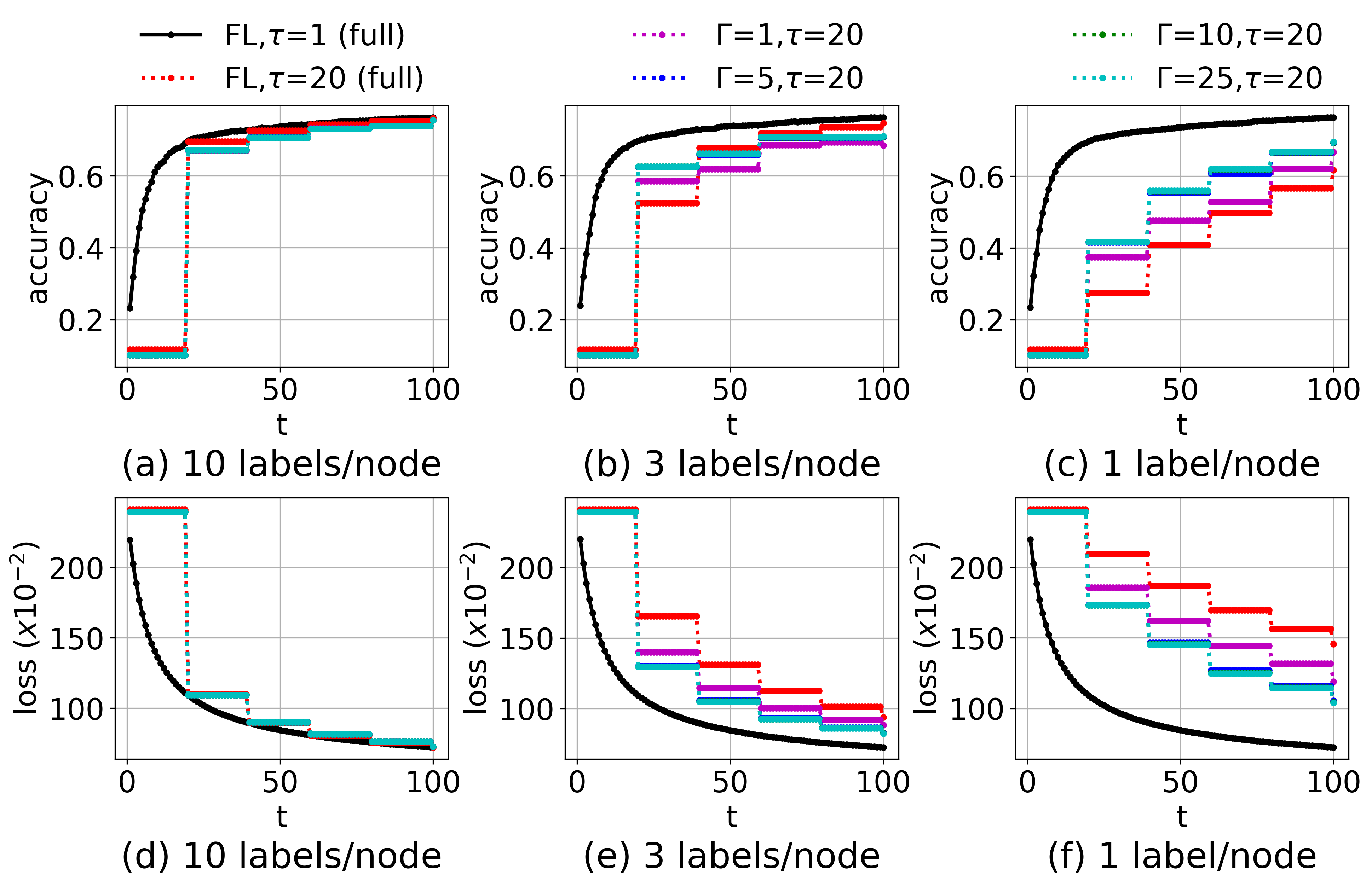
Figure 18: Performance comparison between TT-HF and baseline methods when varying the number of D2D consensus rounds ($\Gamma$). Under the same period of local model training ($\tau$), increasing $\Gamma$ results in a considerable improvement in the model accuracy/loss over time as compared to the current art [16, 58] when data is non-i.i.d. (FMNIST, Neural Network)

• Fig. 5 from main text is repeated in Fig. 9 for FMNIST dataset using SVM, Fig. 14 for MNIST dataset using FCN, and Fig. 18 for FMNIST dataset using FCN.

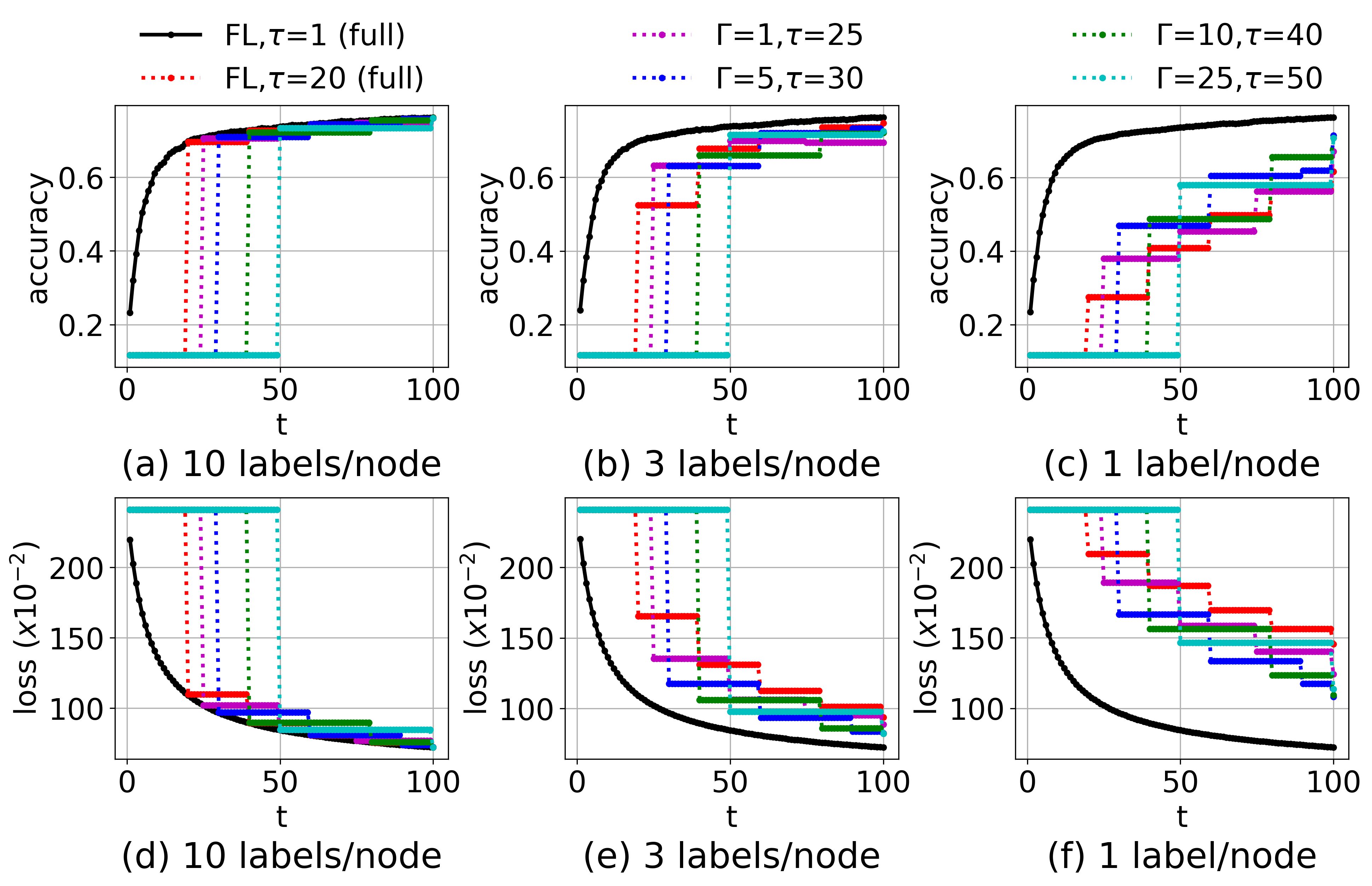
Figure 19: Performance comparison between TT-HF and baseline methods when varying the local model training interval ($\tau$) and the number of D2D consensus rounds ($\Gamma$). With a larger $\tau$, TT-HF can still outperform the baseline federated learning [16, 58] if $\Gamma$ is increased, i.e., local D2D communications can be used to offset the frequency of global aggregations. (FMNIST, Neural Network)

• Fig. 4 from main text is repeated in Fig. 10 for FMNIST dataset using SVM, Fig. 15 for MNIST dataset using FCN, and Fig. 19 for FMNIST dataset using FCN.

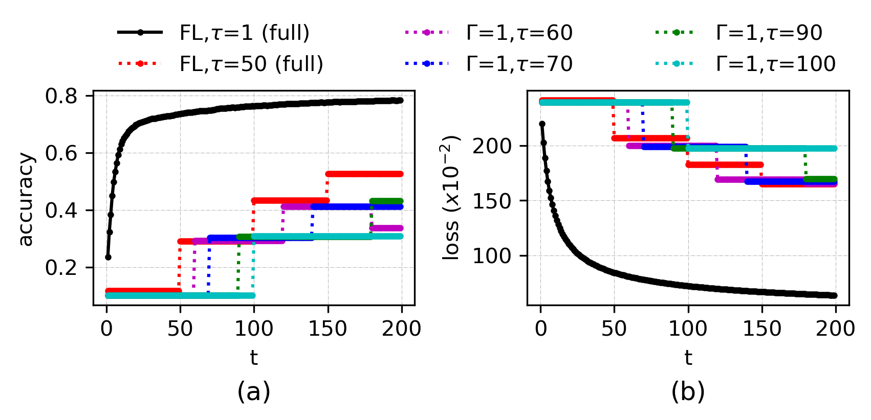
Figure 20: Performance of TT-HF in the extreme non-i.i.d. case for the setting in Fig. 4 when $\Gamma$ is small and the local model training interval length is increased substantially. TT-HF exhibits poor convergence behavior when $\tau$ exceeds a certain value, due to model dispersion. (FMNIST, Neural Network)

• Fig. 6 from main text is repeated in Fig. 11 for FMNIST dataset using SVM, Fig. 16 for MNIST dataset using FCN, and Fig. 20 for FMNIST dataset using FCN.

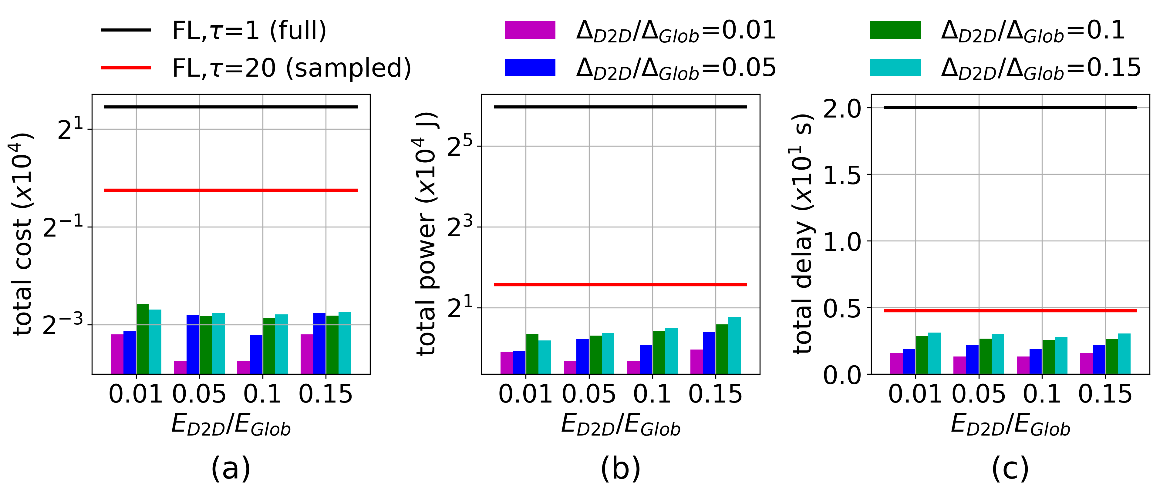
Figure 21: Comparing total (a) cost, (b) power, and (c) delay metrics from the optimization objective in $(\bm{\mathcal{P}})$ achieved by TT-HF versus baselines upon reaching $75\%$ of peak accuracy, for different configurations of delay and energy consumption. TT-HF obtains a significantly lower total cost in (a). (b) and (c) demonstrate the region under which TT-HF attains energy savings and delay gains. (FMNIST, Neural Network)

• Fig. 7 from main text is repeated in Fig. 12 for FMNIST dataset using SVM, Fig. 17 for MNIST dataset using FCN, and Fig. 21 for FMNIST dataset using FCN.

• Fig. 8 from main text is repeated in Fig. 13 for FMNIST dataset using SVM.

Since FCN has a non-convex loss function, Algorithm 2 is not directly applicable for the experiments in Fig. 17&21. As a result, in these cases, we skip the control steps in line 24-25. We instead use a fixed step size, using a constant $\phi$ value to calculate the $\Gamma$’s using (30). We are still able to obtain comparable reductions in total cost compared with the federated learning baselines.

G-B Extension to Other Federated Learning Methods

Although we develop our algorithm based on federated learning with vanilla SGD local optimizer, our method can benefit other counterparts in literature. In particular, we perform some numerical experiments on FedProx [65] to demonstrate the superiority of our semi-decentralized architecture. The performance improvement is due to the fact that, intuitively, conducting D2D communications via the method proposed by us reduces the local bias of the nodes’ models to their local datasets. This benefits the convergence of federated learning methods via counteracting the effect of data heterogeneity across the nodes. The simulation results are provided in Fig. 22 and 23.

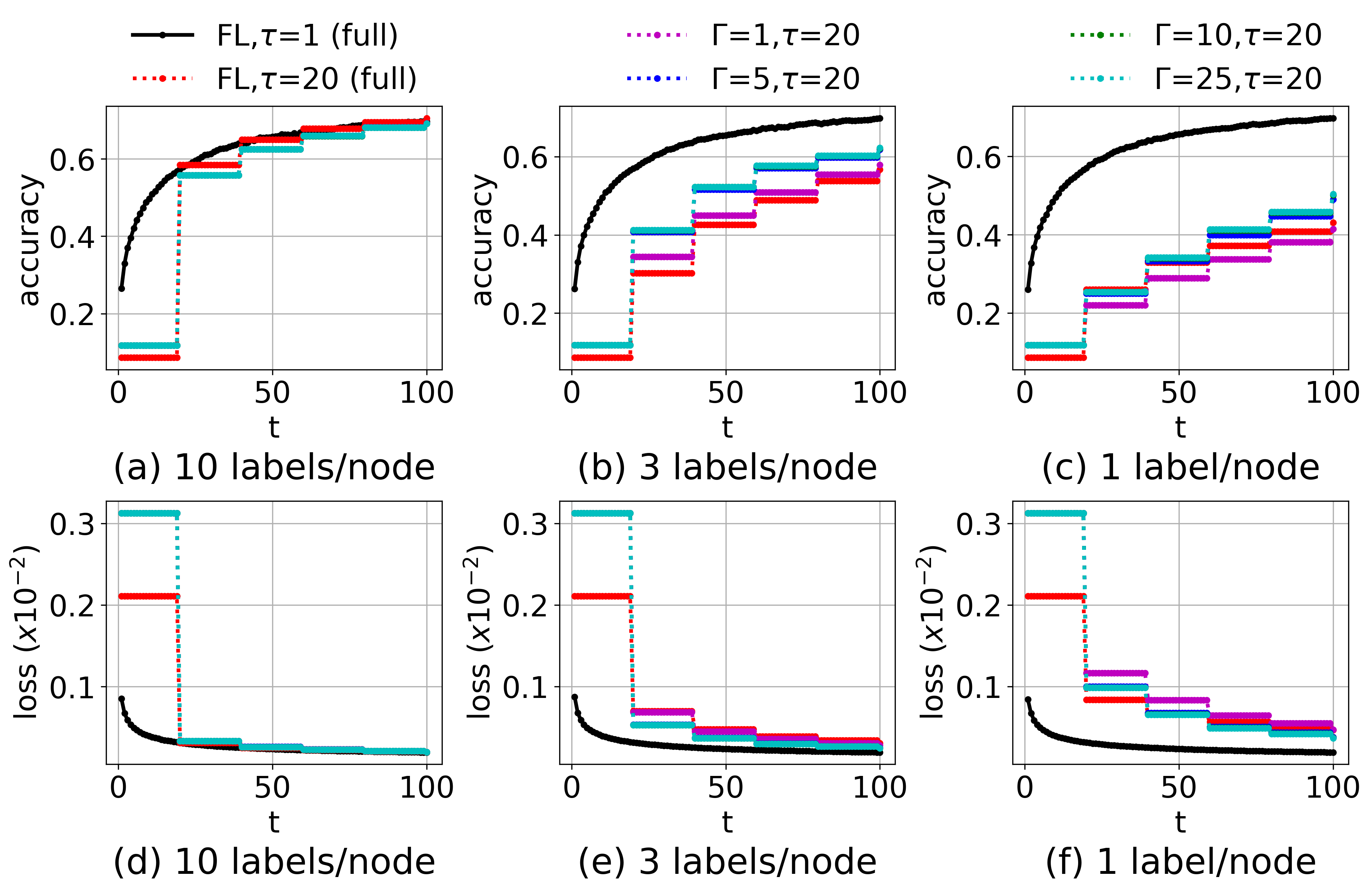
Figure 9: Performance comparison between TT-HF and baseline methods when varying the number of D2D consensus rounds ($\Gamma$). Under the same period of local model training ($\tau$), increasing $\Gamma$ results in a considerable improvement in the model accuracy/loss over time as compared to the current art [16, 58] when data is non-i.i.d. (FMNIST, SVM)

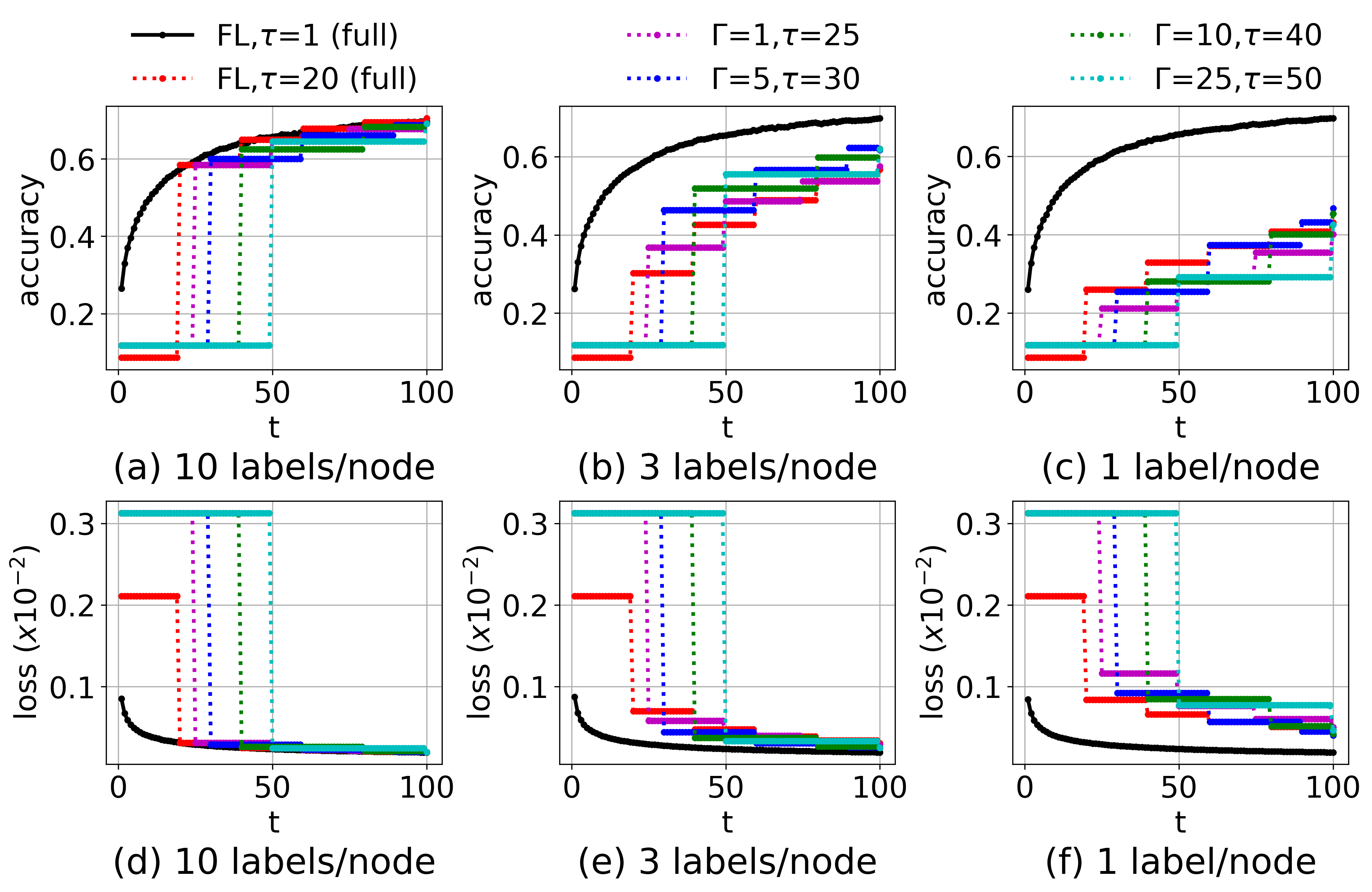
Figure 10: Performance comparison between TT-HF and baseline methods when varying the local model training interval ($\tau$) and the number of D2D consensus rounds ($\Gamma$). With a larger $\tau$, TT-HF can still outperform the baseline federated learning [16, 58] if $\Gamma$ is increased, i.e., local D2D communications can be used to offset the frequency of global aggregations. (FMNIST, SVM)

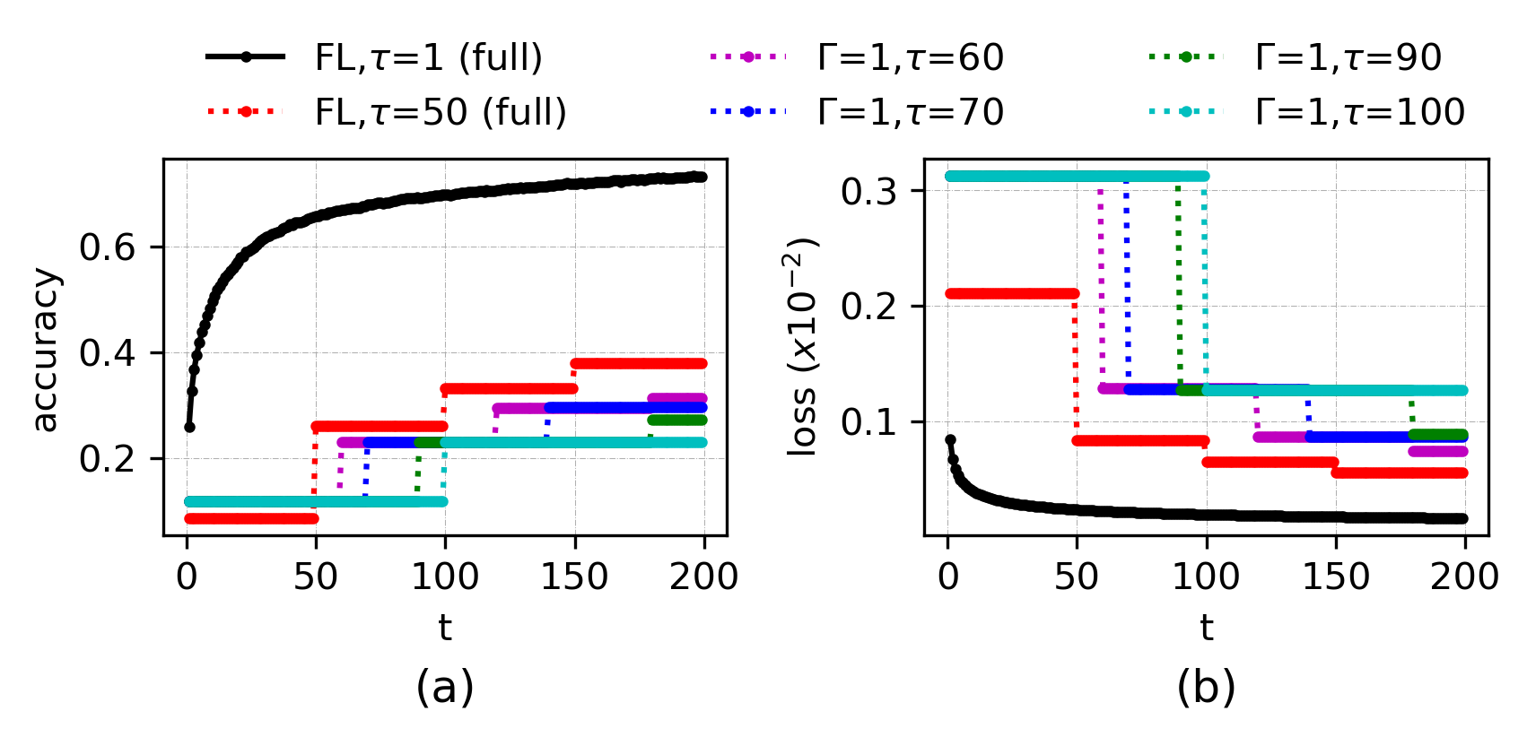
Figure 11: Performance of TT-HF in the extreme non-i.i.d. case for the setting in Fig. 4 when $\Gamma$ is small and the local model training interval length is increased substantially. TT-HF exhibits poor convergence behavior when $\tau$ exceeds a certain value, due to model dispersion. (FMNIST, SVM)

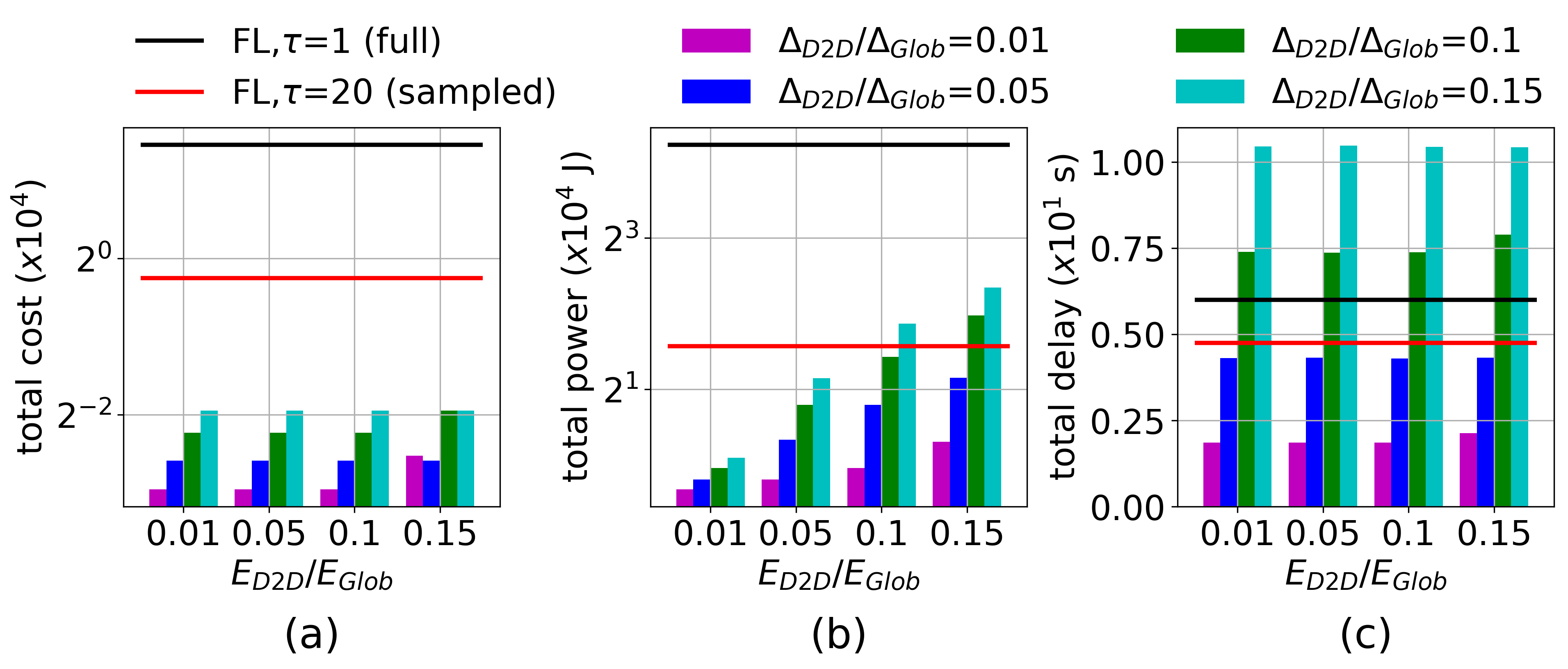
Figure 12: Comparing total (a) cost, (b) power, and (c) delay metrics from the optimization objective in $(\bm{\mathcal{P}})$ achieved by TT-HF versus baselines upon reaching $75\%$ of peak accuracy, for different configurations of delay and energy consumption. TT-HF obtains a significantly lower total cost in (a). (b) and (c) demonstrate the region under which TT-HF attains energy savings and delay gains. (FMNIST, SVM)

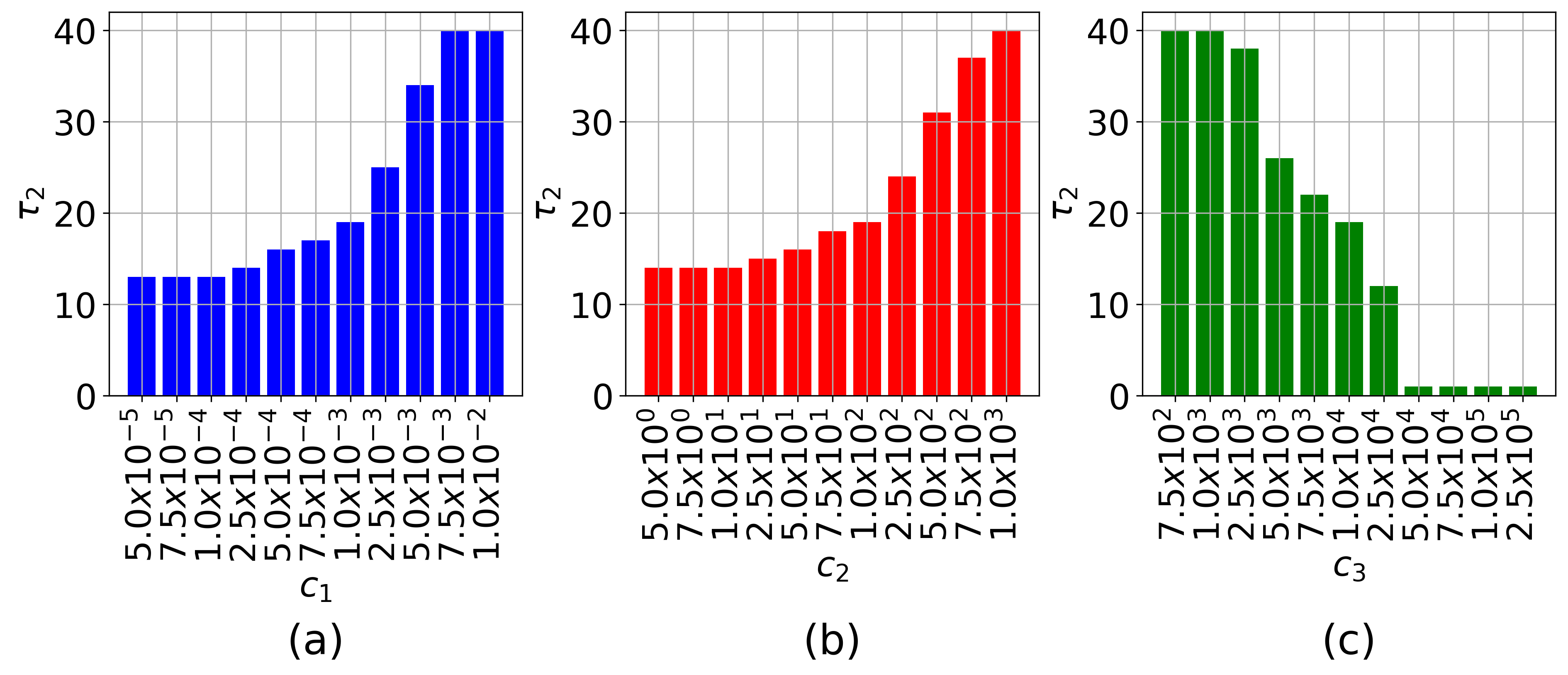
Figure 13: Value of the second local model training interval obtained through $(\bm{\mathcal{P}})$ for different configurations of weighing coefficients $c_{1},c_{2},c_{3}$ (default $c_{1}=10^{-3},c_{2}=10^{2},c_{3}=10^{4}$). Higher weight on energy and delay (larger $c_{1}$ and $c_{2}$) prolongs the local training period, while higher weight on the global model loss (larger $c_{3}$) decreases the length, resulting in more rapid global aggregations. (FMNIST, SVM)

Figure 14: Performance comparison between TT-HF and baseline methods when varying the number of D2D consensus rounds ($\Gamma$). Under the same period of local model training ($\tau$), increasing $\Gamma$ results in a considerable improvement in the model accuracy/loss over time as compared to the current art [16, 58] when data is non-i.i.d. (MNIST, Neural Network)

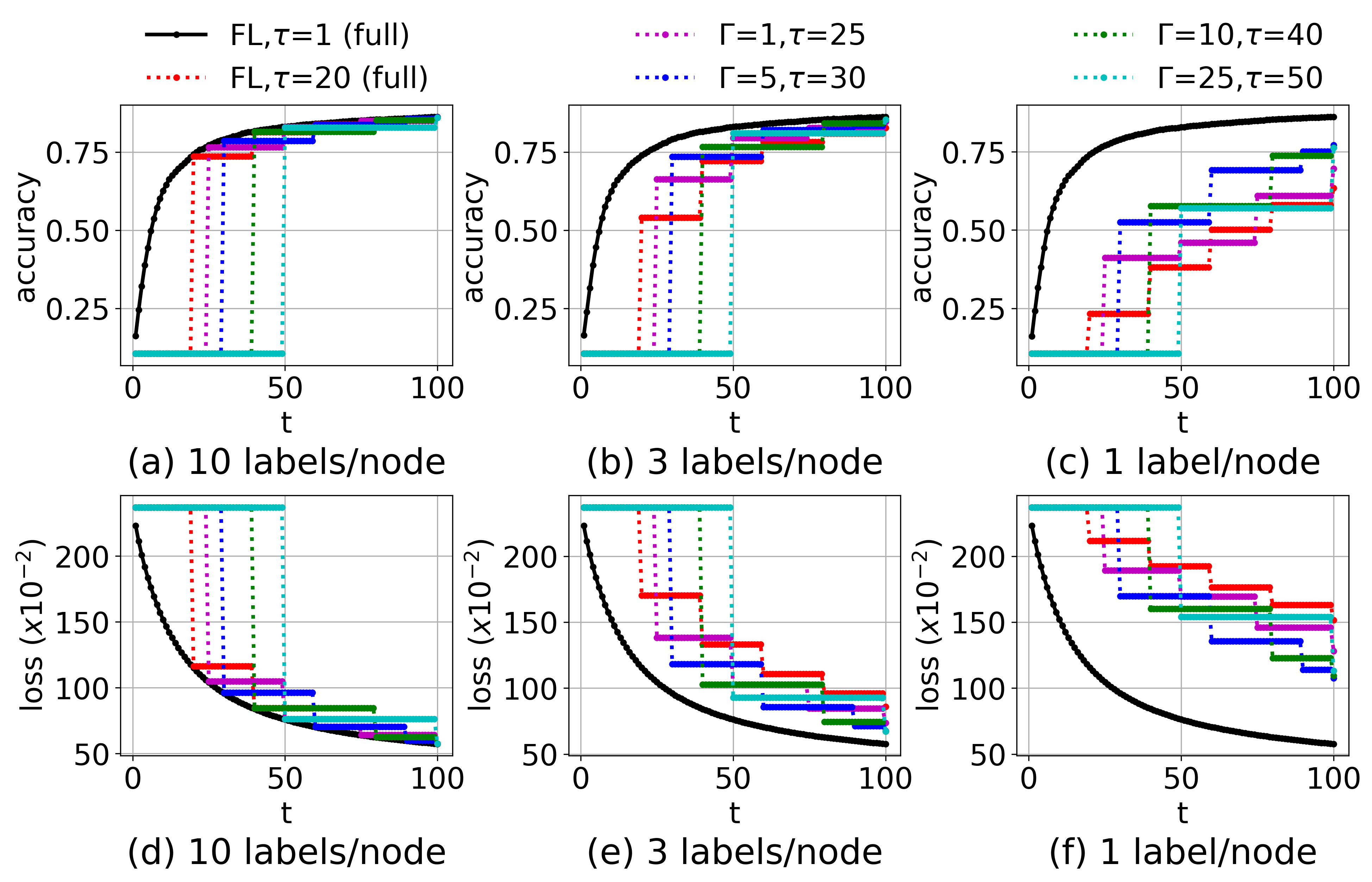
Figure 15: Performance comparison between TT-HF and baseline methods when varying the local model training interval ($\tau$) and the number of D2D consensus rounds ($\Gamma$). With a larger $\tau$, TT-HF can still outperform the baseline federated learning [16, 58] if $\Gamma$ is increased, i.e., local D2D communications can be used to offset the frequency of global aggregations. (MNIST, Neural Network)

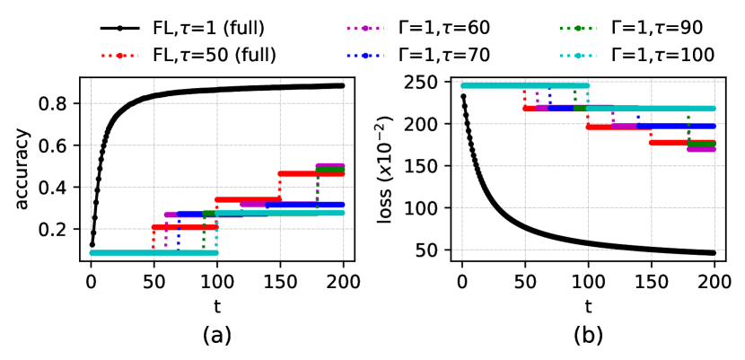
Figure 16: Performance of TT-HF in the extreme non-i.i.d. case for the setting in Fig. 4 when $\Gamma$ is small and the local model training interval length is increased substantially. TT-HF exhibits poor convergence behavior when $\tau$ exceeds a certain value, due to model dispersion. (MNIST, Neural Network)

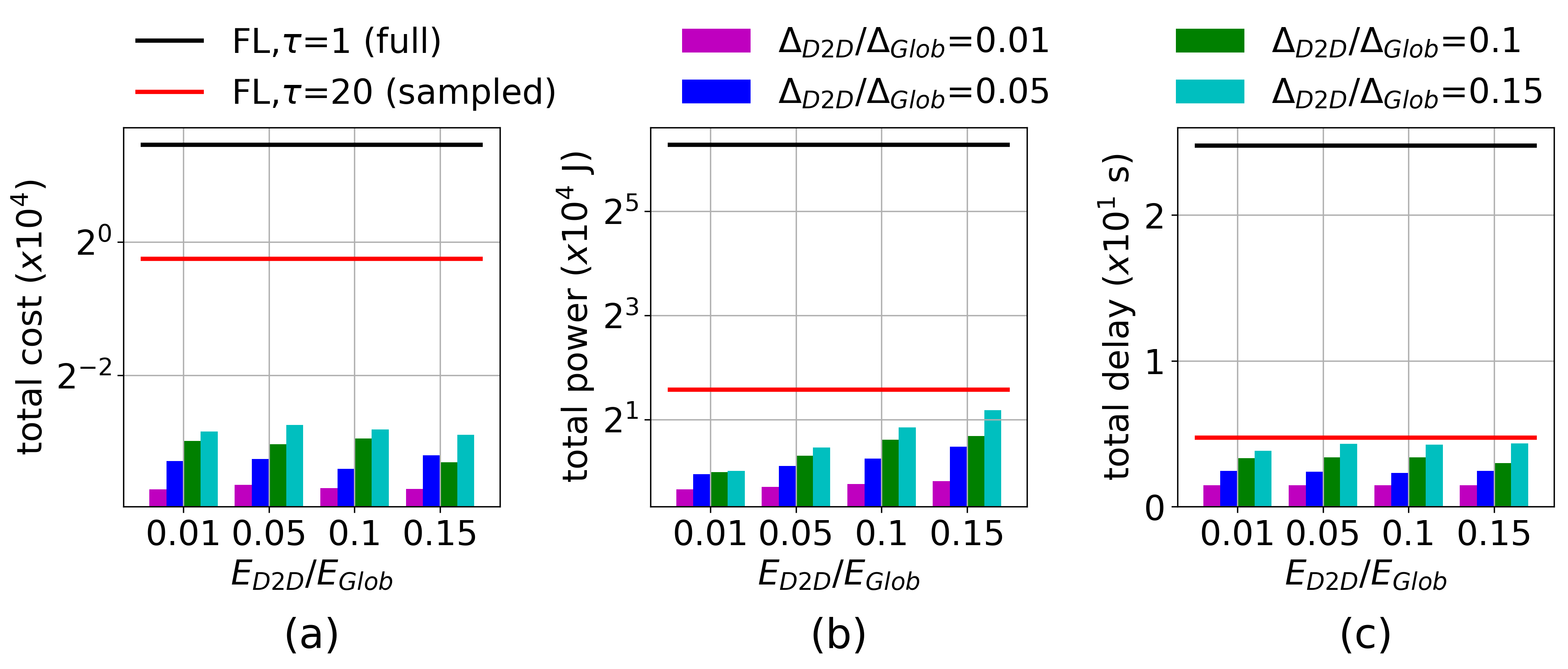
Figure 17: Comparing total (a) cost, (b) power, and (c) delay metrics from the optimization objective in $(\bm{\mathcal{P}})$ achieved by TT-HF versus baselines upon reaching $75\%$ of peak accuracy, for different configurations of delay and energy consumption. TT-HF obtains a significantly lower total cost in (a). (b) and (c) demonstrate the region under which TT-HF attains energy savings and delay gains. (FMNIST, SVM)

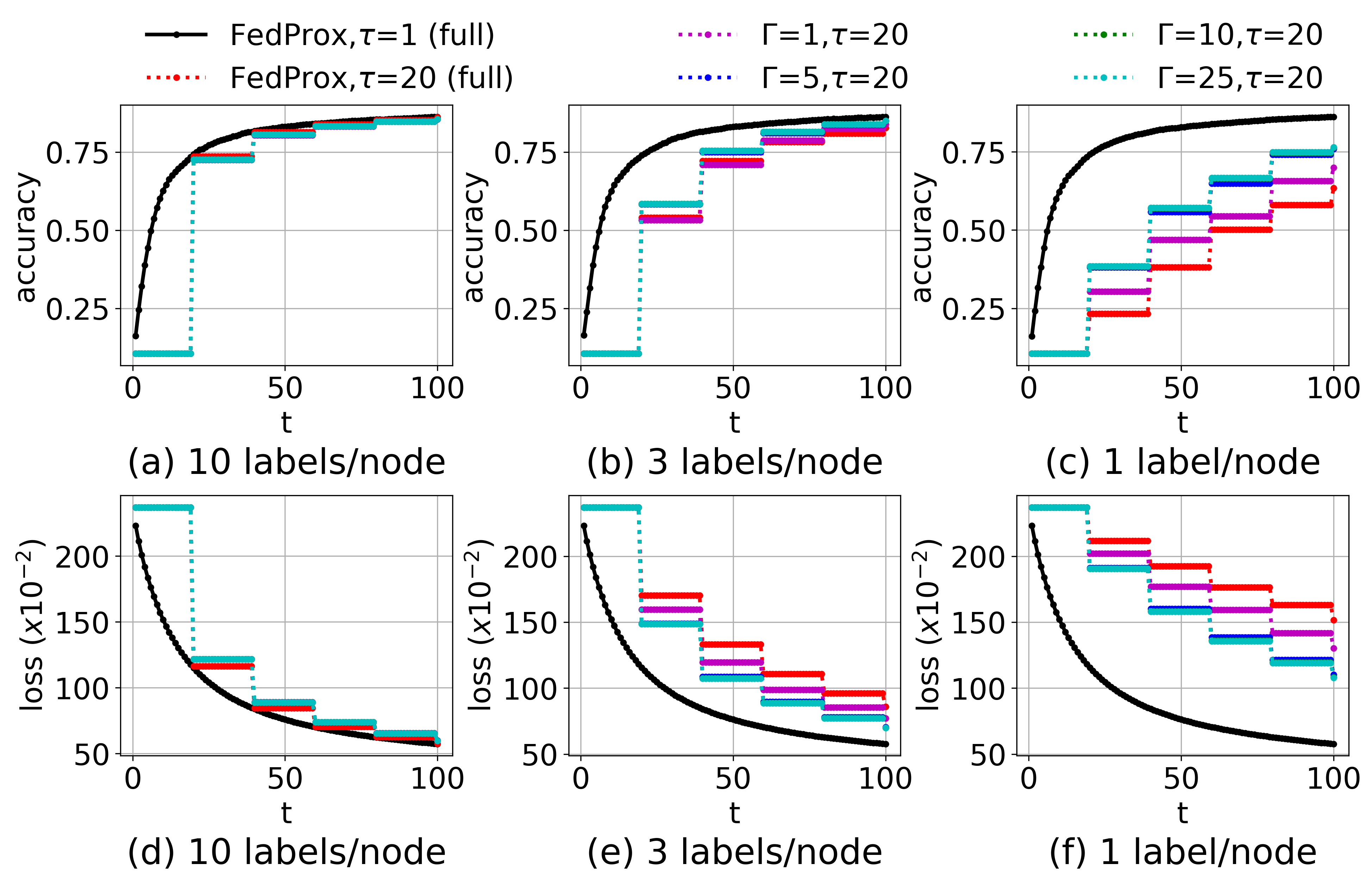
Figure 22: Performance comparison between TT-HF and FedProx [65] when varying the number of D2D consensus rounds ($\Gamma$). Under the same period of local model training ($\tau$), increasing $\Gamma$ results in a considerable improvement in the model accuracy/loss over time as compared to the baseline when data is non-i.i.d. (MNIST, Neural Network)

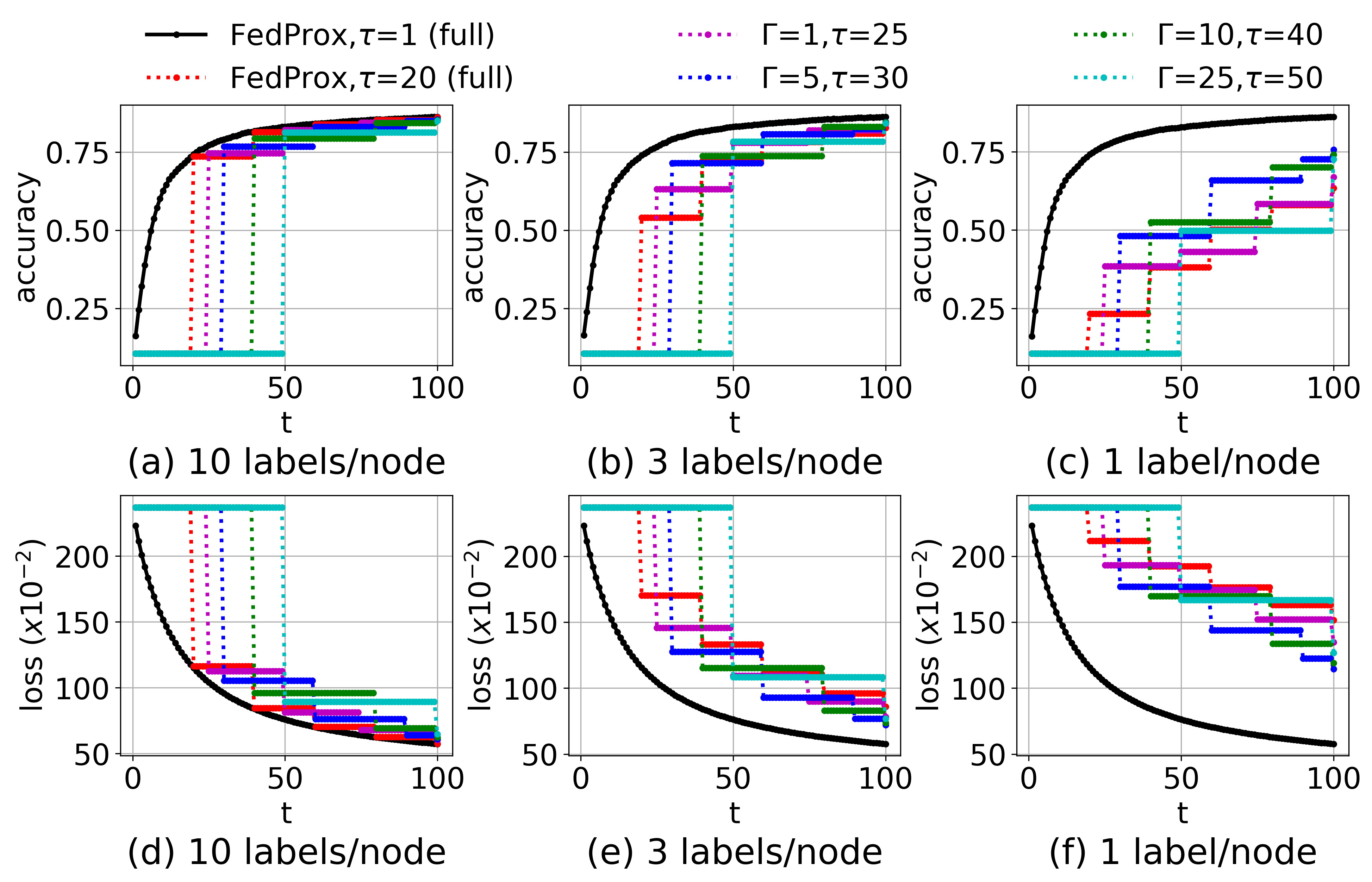
Figure 23: Performance comparison between TT-HF and FedProx [65] when varying the local model training interval ($\tau$) and the number of D2D consensus rounds ($\Gamma$). With a larger $\tau$, TT-HF can still outperform the baseline method if $\Gamma$ is increased, i.e., local D2D communications can be used to offset the frequency of global aggregations. (MNIST, Neural Network)

References

- [1] F. P.-C. Lin, S. Hosseinalipour, S. S. Azam, C. G. Brinton, and N. Michelusi, “Federated learning beyond the star: Local D2D model consensus with global cluster sampling,” in Proc. IEEE Int. Glob. Commun. Conf. (GLOBECOM), 2021, pp. 1–6.
- [2] S. Ghosh, N. Das, I. Das, and U. Maulik, “Understanding deep learning techniques for image segmentation,” ACM Comput. Surveys (CSUR), vol. 52, no. 4, pp. 1–35, 2019.
- [3] K. Kang, W. Ouyang, H. Li, and X. Wang, “Object detection from video tubelets with convolutional neural networks,” in Proc. IEEE Conf. Comput. Vision Pattern Recog. (CVPR), 2016, pp. 817–825.
- [4] Y. Goldberg, “Neural network methods for natural language processing,” Synthesis Lectures on Human Language Technologies, vol. 10, no. 1, pp. 1–309, 2017.
- [5] M. Chiang and T. Zhang, “Fog and iot: An overview of research opportunities,” IEEE Internet Thing J., vol. 3, no. 6, pp. 854–864, 2016.
- [6] B. Wu, F. Iandola, P. H. Jin, and K. Keutzer, “Squeezedet: Unified, small, low power fully convolutional neural networks for real-time object detection for autonomous driving,” in Proc. IEEE Conf. Comput. Vision Pattern Recog. (CVPR) Workshops, 2017, pp. 129–137.
- [7] A. Hard, K. Rao, R. Mathews, S. Ramaswamy, F. Beaufays, S. Augenstein, H. Eichner, C. Kiddon, and D. Ramage, “Federated learning for mobile keyboard prediction,” arXiv preprint arXiv:1811.03604, 2018.
- [8] S. S. Azam, T. Kim, S. Hosseinalipour, C. Brinton, C. Joe-Wong, and S. Bagchi, “Towards generalized and distributed privacy-preserving representation learning,” arXiv preprint arXiv:2010.01792, 2020.
- [9] H. B. McMahan, E. Moore, D. Ramage, S. Hampson, and B. A. y Arcas, “Communication-Efficient Learning of Deep Networks from Decentralized Data,” in Proc. Int. Conf. Artificial Intell. Stat. (AISTATS), 2017.
- [10] J. Konečnỳ, H. B. McMahan, F. X. Yu, P. Richtárik, A. T. Suresh, and D. Bacon, “Federated learning: Strategies for improving communication efficiency,” arXiv preprint arXiv:1610.05492, 2016.
- [11] Q. Yang, Y. Liu, T. Chen, and Y. Tong, “Federated machine learning: Concept and applications,” ACM Trans. Intell. Syst. Technol. (TIST), vol. 10, no. 2, pp. 1–19, 2019.
- [12] W. Y. B. Lim, N. C. Luong, D. T. Hoang, Y. Jiao, Y.-C. Liang, Q. Yang, D. Niyato, and C. Miao, “Federated learning in mobile edge networks: A comprehensive survey,” IEEE Commun. Surveys & Tuts., 2020.
- [13] M. Bennis, M. Debbah, K. Huang, and Z. Yang, “Guest editorial: Communication technologies for efficient edge learning,” IEEE Commun. Mag., vol. 58, no. 12, pp. 12–13, 2020.
- [14] Y. Tu, Y. Ruan, S. Wang, S. Wagle, C. G. Brinton, and C. Joe-Wang, “Network-aware optimization of distributed learning for fog computing,” arXiv preprint arXiv:2004.08488, 2020.
- [15] Z. Yang, M. Chen, W. Saad, C. S. Hong, and M. Shikh-Bahaei, “Energy efficient federated learning over wireless communication networks,” arXiv preprint arXiv:1911.02417, 2019.
- [16] S. Wang, T. Tuor, T. Salonidis, K. K. Leung, C. Makaya, T. He, and K. Chan, “Adaptive federated learning in resource constrained edge computing systems,” IEEE J. Select. Areas Commun., vol. 37, no. 6, pp. 1205–1221, 2019.
- [17] F. P.-C. Lin, C. G. Brinton, and N. Michelusi, “Federated learning with communication delay in edge networks,” in Proc. IEEE Int. Glob. Commun. Conf. (GLOBECOM), 2020, pp. 1–6.
- [18] S. Hosseinalipour, C. G. Brinton, V. Aggarwal, H. Dai, and M. Chiang, “From federated to fog learning: Distributed machine learning over heterogeneous wireless networks,” IEEE Commun. Mag., vol. 58, no. 12, pp. 41–47, 2020.
- [19] M. Chen, H. V. Poor, W. Saad, and S. Cui, “Wireless communications for collaborative federated learning,” IEEE Commun. Mag., vol. 58, no. 12, pp. 48–54, 2020.
- [20] N. H. Tran, W. Bao, A. Zomaya, N. M. NH, and C. S. Hong, “Federated learning over wireless networks: Optimization model design and analysis,” in Proc. IEEE Int. Conf. Comput. Commun. (INFOCOM), 2019, pp. 1387–1395.
- [21] M. Chen, Z. Yang, W. Saad, C. Yin, H. V. Poor, and S. Cui, “A joint learning and communications framework for federated learning over wireless networks,” arXiv preprint arXiv:1909.07972, 2019.
- [22] K. Yang, T. Jiang, Y. Shi, and Z. Ding, “Federated learning via over-the-air computation,” IEEE Trans. Wireless Commun., vol. 19, no. 3, pp. 2022–2035, 2020.
- [23] V. Smith, C.-K. Chiang, M. Sanjabi, and A. S. Talwalkar, “Federated multi-task learning,” in Proc. Adva. Neural Inf. Process. Syst., 2017, pp. 4424–4434.
- [24] L. Corinzia and J. M. Buhmann, “Variational federated multi-task learning,” arXiv preprint arXiv:1906.06268, 2019.
- [25] R. Li, F. Ma, W. Jiang, and J. Gao, “Online federated multitask learning,” in Proc. Int. Conf. Big Data, 2019, pp. 215–220.
- [26] Y. Jiang, J. Konečnỳ, K. Rush, and S. Kannan, “Improving federated learning personalization via model agnostic meta learning,” arXiv preprint arXiv:1909.12488, 2019.
- [27] A. Fallah, A. Mokhtari, and A. Ozdaglar, “Personalized federated learning with theoretical guarantees: A model-agnostic meta-learning approach,” Adv. Neural Inf. Process. Syst., vol. 33, 2020.
- [28] S. A. Rahman, H. Tout, H. Ould-Slimane, A. Mourad, C. Talhi, and M. Guizani, “A survey on federated learning: The journey from centralized to distributed on-site learning and beyond,” IEEE Internet Things J., 2020.
- [29] T. Li, A. K. Sahu, A. Talwalkar, and V. Smith, “Federated learning: Challenges, methods, and future directions,” IEEE Signal Process. Mag., vol. 37, no. 3, pp. 50–60, 2020.
- [30] F. Haddadpour and M. Mahdavi, “On the convergence of local descent methods in federated learning,” arXiv preprint arXiv:1910.14425, 2019.
- [31] L. Liu, J. Zhang, S. Song, and K. B. Letaief, “Client-edge-cloud hierarchical federated learning,” in Proc. IEEE Int. Conf. Commun. (ICC), 2020, pp. 1–6.
- [32] M. M. Amiri, D. Gunduz, S. R. Kulkarni, and H. V. Poor, “Federated learning with quantized global model updates,” arXiv preprint arXiv:2006.10672, 2020.
- [33] F. Sattler, S. Wiedemann, K.-R. Müller, and W. Samek, “Robust and communication-efficient federated learning from non-iid data,” IEEE Trans. Neural Netw. Learn. Syst., vol. 31, no. 9, pp. 3400–3413, 2019.
- [34] N. Yoshida, T. Nishio, M. Morikura, K. Yamamoto, and R. Yonetani, “Hybrid-fl for wireless networks: Cooperative learning mechanism using non-iid data,” in Proc. IEEE Int. Conf. Commun. (ICC), 2020, pp. 1–7.
- [35] S. Wang, M. Lee, S. Hosseinalipour, R. Morabito, M. Chiang, and C. G. Brinton, “Device sampling for heterogeneous federated learning: Theory, algorithms, and implementation,” arXiv preprint arXiv:2101.00787, 2021.
- [36] Y. Zhao, M. Li, L. Lai, N. Suda, D. Civin, and V. Chandra, “Federated learning with non-iid data,” arXiv preprint arXiv:1806.00582, 2018.
- [37] S. Hosseinalipour, S. S. Azam, C. G. Brinton, N. Michelusi, V. Aggarwal, D. J. Love, and H. Dai, “Multi-stage hybrid federated learning over large-scale D2D-enabled fog networks,” arXiv preprint arXiv:2007.09511, 2020.
- [38] H. Xing, O. Simeone, and S. Bi, “Decentralized federated learning via SGD over wireless D2D networks,” in IEEE Int. Workshop Signal Process. Adv. Wireless Commun. (SPAWC), 2020, pp. 1–5.
- [39] S. Savazzi, M. Nicoli, and V. Rampa, “Federated learning with cooperating devices: A consensus approach for massive iot networks,” IEEE Internet Things J., vol. 7, no. 5, pp. 4641–4654, 2020.
- [40] C. Hu, J. Jiang, and Z. Wang, “Decentralized federated learning: a segmented gossip approach,” arXiv preprint arXiv:1908.07782, 2019.
- [41] A. Lalitha, O. C. Kilinc, T. Javidi, and F. Koushanfar, “Peer-to-peer federated learning on graphs,” arXiv preprint arXiv:1901.11173, 2019.
- [42] D. Yuan, S. Xu, and H. Zhao, “Distributed primal–dual subgradient method for multiagent optimization via consensus algorithms,” IEEE Trans. Syst. Man Cybernetics, vol. 41, no. 6, pp. 1715–1724, 2011.
- [43] W. Shi, Q. Ling, K. Yuan, G. Wu, and W. Yin, “On the linear convergence of the ADMM in decentralized consensus optimization,” IEEE Trans. Signal Process., vol. 62, no. 7, pp. 1750–1761, 2014.
- [44] C. S. Lee, N. Michelusi, and G. Scutari, “Finite rate distributed weight-balancing and average consensus over digraphs,” IEEE Trans Autom. Control., pp. 1–1.
- [45] L. Xiao and S. Boyd, “Fast linear iterations for distributed averaging,” Syst. & Control Lett., vol. 53, no. 1, pp. 65–78, 2004.
- [46] M. P. Friedlander and M. Schmidt, “Hybrid deterministic-stochastic methods for data fitting,” SIAM J. Sci. Comput., vol. 34, no. 3, pp. A1380–A1405, 2012.
- [47] H. H. Yang, Z. Liu, T. Q. S. Quek, and H. V. Poor, “Scheduling policies for federated learning in wireless networks,” IEEE Trans. Commun., vol. 68, no. 1, pp. 317–333, 2020.
- [48] C. T. Dinh, N. H. Tran, M. N. H. Nguyen, C. S. Hong, W. Bao, A. Y. Zomaya, and V. Gramoli, “Federated learning over wireless networks: Convergence analysis and resource allocation,” IEEE/ACM Trans. Netw., vol. 29, no. 1, pp. 398–409, 2021.
- [49] M. M. Amiri, D. Gündüz, S. R. Kulkarni, and H. V. Poor, “Convergence of update aware device scheduling for federated learning at the wireless edge,” IEEE Trans. Wireless Commun., vol. 20, no. 6, pp. 3643–3658, 2021.
- [50] M. Chen, H. V. Poor, W. Saad, and S. Cui, “Convergence time minimization of federated learning over wireless networks,” in in IEEE Int. Conf. Commun. (ICC), 2020, pp. 1–6.
- [51] M. Hmila, M. Fernández-Veiga, M. Rodríguez-Pérez, and S. Herrería-Alonso, “Energy efficient power and channel allocation in underlay device to multi device communications,” IEEE Trans. Commun., vol. 67, no. 8, pp. 5817–5832, 2019.
- [52] S. Dominic and L. Jacob, “Joint resource block and power allocation through distributed learning for energy efficient underlay D2D communication with rate guarantee,” Comput. Commun., 2020.
- [53] A. Zhang and X. Lin, “Security-aware and privacy-preserving D2D communications in 5G,” IEEE Netw., vol. 31, no. 4, pp. 70–77, 2017.
- [54] S. Zhang, J. Liu, H. Guo, M. Qi, and N. Kato, “Envisioning device-to-device communications in 6G,” IEEE Netw., vol. 34, no. 3, pp. 86–91, 2020.
- [55] T. Richardson and S. Kudekar, “Design of low-density parity check codes for 5g new radio,” IEEE Commun. Mag., vol. 56, no. 3, pp. 28–34, 2018.
- [56] T. Sery, N. Shlezinger, K. Cohen, and Y. C. Eldar, “Over-the-air federated learning from heterogeneous data,” IEEE Trans. Signal Process., pp. 1–1, 2021.
- [57] S. Bubeck et al., “Convex optimization: Algorithms and complexity,” Found. Trends® Machine Learn., vol. 8, no. 3-4, pp. 231–357, 2015.
- [58] X. Li, K. Huang, W. Yang, S. Wang, and Z. Zhang, “On the convergence of FedAvg on non-iid data,” arXiv:1907.02189, 2019.
- [59] D. Tse and P. Viswanath, Fundamentals of wireless communication. Cambridge university press, 2005.
- [60] J. Kim, S. Hosseinalipour, T. Kim, D. J. Love, and C. G. Brinton, “Multi-IRS-assisted multi-cell uplink MIMO communications under imperfect CSI: A deep reinforcement learning approach,” in IEEE Int. Conf. Commun. Workshop (ICC WKSH), 2021, pp. 1–7.
- [61] L. Yan, C. Corinna, and C. J. Burges. The MNIST dataset of handwritten digits. [Online]. Available: http://yann.lecun.com/exdb/mnist/
- [62] H. Xiao, K. Rasul, and R. Vollgraf. Fashion-MNIST. [Online]. Available: https://github.com/zalandoresearch/fashion-mnist
- [63] K. He, X. Zhang, S. Ren, and J. Sun, “Delving deep into rectifiers: Surpassing human-level performance on imagenet classification,” in Proc. IEEE Int. Conf. Comput. Vision, 2015, pp. 1026–1034.
- [64] [Online]. Available: https://github.com/shams-sam/TwoTimeScaleHybridLearning
- [65] A. K. Sahu, T. Li, M. Sanjabi, M. Zaheer, A. Talwalkar, and V. Smith, “On the convergence of federated optimization in heterogeneous networks,” arXiv preprint arXiv:1812.06127, vol. 3, 2018.